Interfaces and droplets in quantum lattice models

Abstract.

This paper is a short review of recent results on interface states in the Falicov-Kimball model and the ferromagnetic XXZ Heisenberg model. More specifically, we discuss the following topics: 1) The existence of interfaces in quantum lattice models that can be considered as perturbations of classical models. 2) The rigidity of the 111 interface in the three-dimensional Falicov-Kimball model at sufficiently low temperatures. 3) The low-lying excitations and the scaling of the gap in the 111 interface ground state in the ferromagnetic XXZ Heisenberg model in three dimensions. 4) The existence of droplet states in the XXZ chain and their properties.

Introduction

Domain walls or interfaces play an important role in many transport phenomena and are essential for the understanding of dynamical processes such as magnetic ordering and magnetization reversal. In many interesting situations quantum mechanics is important to correctly describe the stability, fluctuations, and excitations of magnetic interfaces, and we expect that this is even more true for a reliable description of the dynamics. Equilibrium states describing interfaces in the Ising model are well-known since the seminal work by Dobrushin [9], and many interesting results on interfaces in classical models have been proved since then. In comparison, there have been very few results for quantum models. In the last few years however, some progress has been made and it is the purpose of this paper to review the main results that have been obtained.

In the next four sections we will discuss the following results:

1. Existence of interfaces in quantum lattice models that can be considered as perturbations of classical models.

2. Rigidity of the 111 interface in the Falicov-Kimball model.

3. Gapless excitations of the 111 interface in the XXZ Heisenberg model.

4. Droplet states in the XXZ chain.

1. Perturbations of classical models

Often, quantum lattice models can be thought of as perturbations of a classical spin system when some parameter in the Hamiltonian is not too large (or too small). Under certain conditions its behavior can then be described by a suitable perturbation theory. The following result is due to Borgs, Chayes, and Fröhlich [5]. In order to simplify the presentation we do not describe the result in its most general form here. Let $n$ be a fixed integer $\geq 2$. For every finite subset $\Lambda\subset\mathbb{Z}^{d}$, let the Hilbert space for the system in volume $\Lambda$ be given by

$$\mathcal{H}_{\Lambda}=\bigotimes_{x\in\Lambda}\mathcal{H}_{x},\quad\mathcal{H}_{x}=\mathbb{C}^{n},\mbox{ for all }x.$$

Consider translation invariant local Hamiltonians of the form

(1.1) $$H_{\Lambda}=\sum_{x,y\in\Lambda,\lvert x-y\rvert=1}h_{xy}+\lambda\sum_{A\subset\Lambda}V_{A}$$

where $h_{xy}$ is a translation invariant isotropic nearest neighbor interaction that is diagonal in a tensor product basis labeled by “classical configurations”, i.e., there is a function $h(\sigma_{0},\sigma_{1})$, such that $h_{xy}\lvert\sigma\rangle=h(\sigma_{x},\sigma_{y})\lvert\sigma\rangle$. Here, $\sigma=\{\sigma_{x}\}_{x\in\Lambda},1\leq\sigma_{x}\leq n$, and $\lvert\sigma\rangle=\bigotimes_{x\in\Lambda}\lvert\sigma_{x}\rangle\in\mathcal{H}_{\Lambda}$, and $\{\lvert 1\rangle,\ldots,\lvert n\rangle\}$ is a basis of $\mathbb{C}^{n}$. Assume that this classical nearest neighbor interaction has exactly two ground state, of the form $\lvert\sigma_{0}\rangle\otimes\lvert\sigma_{0}\rangle$. The quantum perturbation given by the $V_{A}$ is also assumed to be translation invariant and sufficiently short range in the sense that, for some $r\geq 0$, sufficiently large,

$$\sum_{A\subset\mathbb{Z}^{d},\,0\in A}\|V_{A}\|e^{rD(A)}<+\infty$$

where $\|\,\cdot\,\|$ is the usual operator norm, and $D(A)$ is the size of the smallest tree subgraph of $\mathbb{Z}^{d}$ containing the vertices of $A$.

Theorem 1.1 (Borgs-Chayes-Fröhlich [5]).

Under the assumptions described above, and if $d\geq 3$, the model defined by (1.1) has Gibbs states with a rigid interface in the principle coordinate directions, provided that the inverse temperature $\beta$ is sufficiently large and $\beta\lambda$ is sufficiently small.

The proof of this theorem relies on recently developed techniques to derive Pirogov-Sinai type results for quantum lattice models [7, 6].

The next two results are examples of interesting situations where perturbation theory as described above, does not apply. They also illustrate two features that distinguish quantum models from their classical counterparts: 1) in a system that has classically several equivalent energy minimizing configurations, ground state selection will typically occur in the quantum model in the same way as tunneling in a symmetric double well potential leads to a unique ground state, and 2) finite-state models can have continuous symmetries and gapless energy spectra.

2. Rigidity of the 111 interface in the Falicov-Kimball model

It is expected that the three-dimensional Ising model does not have Gibbs states with an interface in the 111 direction, due to a large ground state degeneracy for the obvious boundary conditions that would favor such an interface. A proof of the Solid-on-Solid version of this statement was given by Kenyon [14]. In contrast, in the Falicov-Kimball and Heisenberg XXZ models, in dimensions $\geq 2$, this degeneracy is lifted by the “quantum” terms, i.e., ground state selection occurs. Our next result is that, for the half-filled, neutral Falicov-Kimball model in three dimensions the 111 interface is rigid at sufficiently low temperatures [8].

The Falicov-Kimball model consists of two subsystems living on the same lattice $\mathbb{Z}^{d}$: “ions”, described by Ising type variables $W(x)\in\{0,1\}$, and “electrons”, described by fermion operators $c^{+}_{x},c_{x}$. The ions and electrons interact via an on-site Coulomb term as in the Hubbard model. The local Hamiltonians are

(2.1) $$H_{\Lambda}=-\sum_{\{x,y\}\subset\Lambda,|x-y|=1}c^{+}_{x}c_{y}+2U\sum_{x\in\Lambda}W(x)c^{+}_{x}c_{x}$$

We only consider the half-filled neutral case, i.e., the number of ions and the number of electrons are both taken to be equal to half the number of lattice sites and we take $U>0$. Kennedy and Lieb proved that, for $d\geq 2$, this model has an Ising type phase transition, with two low-temperature phases dominated by the two checkerboard configurations for the ions [13].

In order to study the 111 interface in the three-dimensional model, we integrate out the fermion degrees of freedom using the methods of Messager and Miracle-Solé [20], and obtain an effective Hamiltonian for the ions in terms of the the Ising variables $s_{x}=(-1)^{|x|}(2W(x)-1)$:

$$H^{\rm eff}_{\Lambda}(\{s_{x}\})=-J(U,\beta)\sum_{\{x,y\}\cap\Lambda\neq\emptyset,|x-y|=1}s_{x}s_{y}+\sum_{B\cap\Lambda\neq\emptyset,|B|\geq 2}R_{B}(U)$$

where, and $0<J(U,\beta)=1/(4U)+$ terms of higher order in $U^{-1}$ starting with $U^{-3}$ and also including a weak $\beta$ dependence. $R_{B}$ depends on $\{s_{x}\mid x\in B\}$, is translation covariant and satisfies

$$\sum_{B\ni 0}|R_{B}|e^{rn(B)}<\infty$$

for some $r>0$, and where $n(B)$ is the length of the shortest closed path in the lattice visiting all sites in $B$ at least once, and where $R_{B}$ satisfies a bound of the form

$$\lvert R_{B}(U)\rvert\leq\mbox{constant}\times\left(\frac{\rm constant}{U}\right)^{n(B)-1}.$$

Analysis of the terms with $n(B)=4$, indicates that ground state selection indeed occurs for the model with 111 boundary conditions. The following theorem shows that the 111 interface is stable against thermal fluctuations at sufficiently low temperatures.

Theorem 2.1 (Datta-Messager-Nachtergaele [8]).

There exist constants $U_{0}$, $\!C$, $c$, and $D$, such that for all $U>U_{0}$, and $\beta>DU^{3}$, there exists a Gibbs state $\omega_{111}$ of the half-filled neutral three-dimensional Falicov-Kimball model defined by (2.1) with the following properties:

$$\omega_{111}(s_{x})\geq\phantom{-}1-Ce^{-c\beta/U^{3}} x_{1}+x_{2}+x_{3}\geq 1$$ if

$$\omega_{111}(s_{x})\leq-1+Ce^{-c\beta/U^{3}} x_{1}+x_{2}+x_{3}\leq-1$$ if

The Falicov-Kimball model also exhibits phase separation, i.e., spontaneous formation of domains of different phases, in the ground state for certain intervals of densities [11, 12].

3. Gapless excitations of the 111 interface in the XXZ Heisenberg model

The spin 1/2 XXZ Heisenberg model defined by

(3.1) $$H_{\Lambda}=-\sum_{x,y\in\Lambda,|x-y|=1}\frac{1}{\Delta}(S_{x}^{1}S_{y}^{1}+S_{x}^{2}S_{y}^{2})+S_{x}^{3}S_{y}^{3}$$

with $\Delta>1$, can also be regarded as a perturbation of the Ising model. Kennedy proved that this model has a phase transition for all $d\geq 2$, $\Delta>1$ [11]. Theorem 1.1 applies and interface states in the principal coordinate directions exist for $d\geq 3$, and $\beta$ and $\beta/\Delta$ large enough. One can also show that for $d\geq 2$, ground state selection occurs for suitable conditions that favor a diagonal (11, 111, etc.) interface. The model differs from the Falicov-Kimball model, however, in one important aspect: the existence of a diagonal interface is accompanied by the breaking of a continuous symmetry (rotations about the third axis), and consequently has a gapless spectrum above the ground states. These gapless excitations were first described by Koma and Nachtergaele in the two-dimensional case [16, 17]. Matsui proved their existence in all dimensions $\geq 2$ [19].

I conjecture that the XXZ model has a 111 interface Gibbs state in three dimensions at low temperatures. This cannot be proved using the standard expansion techniques, which all rely on the existence of a gap. Therefore, it is reasonable to first try to understand the gapless excitations of the model.

The third component of the total spin or, equivalently, the number of down spins, is a conserved quantity of the XXZ model. Therefore, it is natural to consider the interface problem and the excitation spectrum in the canonical ensemble where this quantity is fixed. The following theorem holds in the canonical ensemble. An equivalence-of-ensembles result is an essential part of its proof.

Theorem 3.1 (Bolina-Contucci-Nachtergaele-Starr [3]).

Let $0<q<1$ be such that $\Delta=(q+q^{-1})/2$. Then the XXZ model with Hamiltonian (3.1), possesses excitations localized in a cylinder with axis in the 111 direction and with a circular intersection of radius $R$ with the interface with the energy gap $\gamma_{R}$ bounded by

$$\gamma_{R}\leq 100\frac{q^{2(1-\delta(q,\nu))}}{(1-q^{2})}\frac{1}{R^{2}},\quad\textrm{for}\quad R>70,$$

where $\delta(q,\nu)$ is an exponent between $0$ and $1/2$, depending on the filling factor $\nu$ of the interface plane and the parameter $q\in(0,1)$.

See [2, 3, 4] for more details and related results.

4. Droplet states in the XXZ chain

The last result we would like to present is concerned with droplet states rather than interfaces. One does not expect that a localized droplet in a translation invariant system can be described by a stationary state, i.e., an eigenvector, of the Hamiltonian. On the other hand, it seems obvious that for a ferromagnetic model such as the XXZ Heisenberg Hamiltonian, any state of a given finite energy in a sufficiently large volume should be a superposition of states that predominantly consist of a small number of domains each described by one of the ground states. We have obtained an explicit result of this kind in the one-dimensional case.

Let $H^{++}_{[1,L]}$ be the following Hamiltonian with “+” boundary fields for a chain of $L$ spins:

(4.1) $$H^{++}_{[1,L]}=-\sum_{x=1}^{L}\frac{1}{\Delta}(S_{x}^{1}S_{x+1}^{1}+S_{x}^{2}S_{x+1}^{2})+(S_{x}^{3}S_{x+1}^{3}-\frac{1}{4})-A(\Delta)(S^{3}_{1}+S^{3}_{L}),$$

where $S^{i}_{x}$ are the standard spin-1/2 matrices and $A(\Delta)=\frac{1}{2}\sqrt{1-\Delta^{-2}}$. $H^{++}_{[1,L]}$ commutes with $\sum_{x=1}^{L}S_{n}^{3}$, and therefore the subspaces $\mathcal{H}_{L,n}$ of $\mathcal{H}_{[1,L]}$ consisting of all states with a fixed number, $n$, of down spins, are invariant. The ground state in each of these invariant subspaces is a delocalized droplet of $n$ down spins, i.e., this ground state is dominated by configurations where all $n$ down spins are in a subinterval of length $n+O(1)$, but all such intervals are roughly equally probable. Thus, we expect that the droplet of size $n$ behaves as a particle freely moving in an interval of length $L-n+1$. Our results on the spectrum show that this particle has mass of order $q^{-n}$, where $q\in(0,1)$ is related to the anisotropy by $\Delta=(q+q^{-1})/2$. To state the precise result, let $\lambda_{L,n}(1)\leq\lambda_{L,n}(2)\leq\dots$ denote the eigenvalues of $H^{++}_{[1,L]}$ restricted to $\mathcal{H}_{L,n}$, and let $\psi^{++}_{L,n}(1),\psi^{++}_{L,n}(2),\dots$ be the corresponding eigenvectors. It is convenient, though not necessary, to describe the spectral projection corresponding to the $L-n+1$ lowest eigenvalues rather than the individual eigenvectors. Define

$$\mathcal{H}^{k}_{L,n}={\rm span}\{\psi^{++}_{L,n}(j):1\leq j\leq k\}\,.$$

and denote by ${\rm Proj}(\mathcal{H}^{k}_{L,n})$ the corresponding orthogonal projection. We have no exact expressions for the this spectral projection for finite $n$, but we can describe it with an error of no more than order $q^{n/2}$ in the operator norm. To state the result we need to introduce the “droplet” subspace of $\mathcal{H}_{L,n}$. We start with the definition of the kink and antikink states, which are ground state of the model with a different choice of boundary fields [1, 10]. For every interval $[a,b]\subset\mathbb{Z}$, and $n=0,1,\ldots,b-a+1$, the kink and antikink states, $\psi^{+-}_{[a,b]}(n)$ and $\psi^{-+}_{[a,b]}(n)$ respectively, are given by the following expressions:

$$\psi^{+-}_{[a,b]}(n)=\sum_{a\leq x_{1}<\dots<x_{n}\leq b}q^{\sum_{k=1}^{n}(b+1-x_{k})}\left(\prod_{k=1}^{n}S_{x_{k}}^{-}\right)\lvert\uparrow\dots\uparrow\rangle_{[a,b]}$$

$$\psi^{-+}_{[a,b]}(n)=\sum_{a\leq x_{1}<\dots<x_{n}\leq b}q^{\sum_{k=1}^{n}(x_{k}+1-a)}\left(\prod_{k=1}^{n}S_{x_{k}}^{-}\right)\lvert\uparrow\dots\uparrow\rangle_{[a,b]}$$

We now define the “droplet” states, describing a localized droplet of size $n$ centered at $x$: for $n\geq 0$ and $\left\lfloor{n/2}\right\rfloor\leq x\leq L-\left\lceil{n/2}\right\rceil$ define

(4.2) $$\xi_{L,n}(x)\ =\psi^{+-}_{[1,x]}(\left\lfloor{n/2}\right\rfloor)\otimes\psi^{-+}_{[x+1,L]}(\left\lceil{n/2}\right\rceil)\,.$$

Here, for any real number $x$, $\left\lfloor{x}\right\rfloor$ is the greatest integer $\leq x$, and $\left\lceil{x}\right\rceil$ is the least integer $\geq x$. The droplet subspace is now defined as the span of the droplet states at all possible positions:

(4.3) $$\mathcal{K}_{L,n}={\rm span}\{\xi_{L,n}(x):\,\left\lfloor{n/2}\right\rfloor\leq x\leq L-\left\lceil{n/2}\right\rceil\}\,.$$

Note that $\dim\mathcal{K}_{L,n}=L-n+1$, which is the number of subintervals of length $n$ of an interval of length $L$. The orthogonal projection onto $\mathcal{K}_{L,n}$ is denoted by ${\rm Proj}(\mathcal{K}_{L,n})$.

Theorem 4.1 (Nachtergaele-Starr [21]).

1. The first $L-n+1$ eigenvalues of $H^{++}_{[1,L]}$ restricted to $\mathcal{H}_{L,n}$ are all approximately equal to $A(\Delta)$. More precisely we have the following:

   $$\lambda_{L,n}(1),\dots,\lambda_{L,n}(L-n+1)\in[A(\Delta)-O(q^{n}),A(\Delta)+O(q^{n})]\,.$$

2. For sufficiently large $n$, the first $L-n+1$ eigenvalues are separated from the rest of spectrum by a gap of approximate magnitude $\gamma=1-\Delta^{-1}$:

   $$\lambda_{L,n}(L-n+2)\geq A(\Delta)+\gamma-O(n^{-1/4}).$$

3. The spectral subspace $\mathcal{H}^{L-n+1}_{L,n}$ spanned by the first $L-n+1$ eigenvectors, for sufficiently large $n$, is close to the space $\mathcal{K}_{L,n}$ defined in (4.3). More precisely we have the the following bound on the norm of the difference of the corresponding projections:

   $$\|{\rm Proj}(\mathcal{K}_{L,n})-{\rm Proj}(\mathcal{H}^{L-n+1}_{L,n})\|=O(q^{n/2})\,.$$

The gap of approximately $\gamma=1-\Delta^{-1}$ shown in part (b) of the Theorem is the energy required to overturn one spin in either the interior or the exterior of the droplet [15, 18]. This energy is less than the energy required to create an additional droplet at infinite distance, which is $2A(\Delta)$, i.e., droplets attract.

Part (c) of the Theorem means that the eigenvectors can be approximated by a superposition of the states $\xi_{L,n}(x)$, which in turn are given by an explicit formula, with increasing accuracy as $n\to\infty$. Note that the Theorem also implies that, for any sequence of states with energies converging to $A(\Delta)$, we must have that the distances of these states to the subspaces $\mathcal{K}_{L,n}$ converges to zero, i.e., in the limit the states contain exactly one droplet, which may either be localized or not.

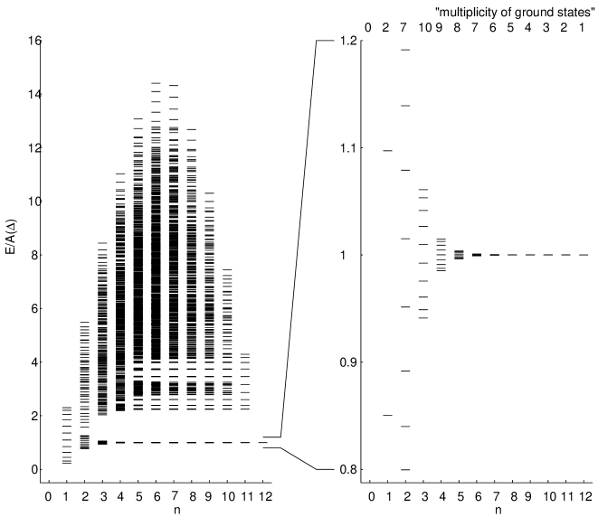
Figure 1. Spectrum for $H^{++}_{[1,12]}$ when $\Delta=2.125$ ($q=1/4$). The (trivial) $n=0$ state is not shown. Its energy is $-A(\Delta)$.

Figure 1 illustrates these features of the spectrum for $L=12$ and $\Delta=2.125$. The multiplet of droplet states is clearly visible, as well as the gap above it.

References

- [1] F.C. Alcaraz, S.R. Salinas, and W.F. Wreszinski, Anisotropic ferromagnetic quantum domains, Phys. Rev, Lett. 75 (1995), 930–933.
- [2] O. Bolina, P. Contucci, and B. Nachtergaele, Path integral representation for interface states of the anisotropic Heisenberg model, to appear in Rev. Math. Phys., arXiv:math-ph/9908004.
- [3] O. Bolina, P. Contucci, B. Nachtergaele, and S. Starr, Finite-volume excitations of the 111 interface in the quantum XXZ model, Comm. Math. Phys. 212 (2000), 63–91, arXiv:math-ph/9908018.
- [4] O. Bolina, P. Contucci, B. Nachtergaele, and S. Starr, A continuum approximation for the excitations of the interface in the quantum Heisenberg model, Electronic Journal of Differential Equations, Conf. 04, (2000), 1-10, arXiv:math-ph/9909018.
- [5] C. Borgs, J. Chayes, and J. Fröhlich, Dobrushin states in quantum lattice systems, Commun. Math. Phys. 189 (1997), 591–619.
- [6] C. Borgs, R. Kotecký, and D. Ueltschi, Low temperature phase diagrams of quantum perturbations of classical spin systems, Commun. Math. Phys., 181 (1996) 409–446.
- [7] N. Datta, R. Fernández, and J. Fröhlich, Low-temperature phase diagrams of quantum lattice systems. I. Stability for quantum perturbations of classical systems with finitely-many ground states, J. Stat. Phys. 84 (1996), 455–534.
- [8] N. Datta, A. Messager, and B. Nachtergaele, Rigidity of the 111 interface in the Falicov-Kimball model, J. Stat. Phys., 99 (2000), 461-555, arXiv:math-ph/9804008.
- [9] R.L. Dobrushin, Gibbs state describing the coexistence of phases for a three–dimensional Ising model, Theor. Prob. Appl. 17 (1972), 582.
- [10] C.-T. Gottstein, R.F. Werner, Ground states of the infinite q-deformed Heisenberg ferromagnet, arXiv:cond-mat/9501123.
- [11] T. Kennedy, Phase separation in the neutral Falicov-Kimball model, J. Stat. Phys. 91 (1998), 829–843, arXiv:cond-mat/9705315.
- [12] T. Kennedy and K. Haller, Periodic Ground States in the Neutral Falicov-Kimball Model in Two Dimensions, submitted to J. Stat. Phys., arXiv:cond-mat/0004104.
- [13] T. Kennedy and E. H. Lieb, An itinerant electron model with crystalline or magnetic long-range order, Physica 138A (1986), 320–358.
- [14] R. Kenyon, Local statistics of lattice dimers, Ann. Inst. H. Poincaré, Probab. Statist., 33 (1997), 591–618.
- [15] T. Koma and B. Nachtergaele, The spectral gap of the ferromagnetic XXZ chain, Lett. Math. Phys. 40 (1997), 1–16.
- [16] T. Koma and B. Nachtergaele, Low-lying spectrum of quantum interfaces, Abstracts of the AMS, 17 (1996), 146, and unpublished notes.
- [17] T. Koma and B. Nachtergaele, Interface states of quantum lattice models, In Matsui, T. (eds.) Recent Trends in Infinite Dimensional Non-Commutative Analysis. RIMS Kokyuroku # 1035, Kyoto, 1998, 133–144.
- [18] T. Koma and B. Nachtergaele, The complete set of ground states of the ferromagnetic XXZ chains, Adv. Theor. Math. Phys., 2 (1998), 533–558, arXiv:cond-mat/9709208
- [19] T. Matsui, On the spectra of the kink for ferromagnetic models, Lett. Math. Phys. 42 (1997), 229–239.
- [20] A. Messager and S. Miracle-Solé, Low temperature states in the Falikov-Kimbal model, Rev. Math. Phys. 8 (1996) 271–299.
- [21] B. Nachtergaele and S. Starr, Droplet states of the XXZ Heisenberg chain, arXiv:math-ph/0009002.