Hamiltonian self-adjoint extensions for (2+1)-dimensional Dirac particles

Abstract

Abstract: We study the stationary problem of a charged Dirac particle in (2+1)-dimensions in the presence of a uniform magnetic field $B$ and a singular magnetic tube of flux $\Phi=2\pi\kappa/e$. The rotational invariance of this configuration implies that the subspaces of definite angular momentum $l+1/2$ are invariant under the action of the Hamiltonian $H$. We show that, for $\kappa-l\geq 1$ or $\kappa-l\leq 0$, the restriction of $H$ to these subspaces, $H_{l}$, is essentially self-adjoint, while for $0<\kappa-l<1$, $H_{l}$ admits a one-parameter family of self-adjoint extensions (SAE). In the later case, the functions in the domain of $H_{l}$ are singular (but square-integrable) at the origin, their behavior being dictated by the value of the parameter $\gamma$ that identifies the SAE. We also determine the spectrum of the Hamiltonian as a function of $\kappa$ and $\gamma$, as well as its closure.

I Introduction

In Quantum Mechanics, observables are realized in terms of self-adjoint operators on a Hilbert space. It is for these operators that the spectral theorem holds [1]. In particular, the dynamics of a quantum system should be given by a unitary group whose generator, the Hamiltonian $H$ (usually a differential operator acting on an appropriate space of square integrable functions), must be self-adjoint.

In general, physical considerations lead to a formal expression for the Hamiltonian, although they can leave its domain of definition not completely specified. Usually, one can choose a dense subspace of the Hilbert space on which $H$ is well-defined and symmetric, but not necessarily self-adjoint.

In these conditions, the question is posed of determining if the expression found for $H$ has a unique self-adjoint extension in the Hilbert space (i.e., if $H$ is essentially self-adjoint), or it admits different self-adjoint extensions (SAE) (differing in the physics they describe) and, in this case, which one corresponds to the physical system under consideration.

A situation of practical interest in which the Hamiltonian admits nontrivial self-adjoint extensions corresponds to the movement of charged particles under the influence of a Bohm - Aharonov singular magnetic flux tube [2], like fermions in the presence of cosmic strings [3] or non-relativistic spinless quantum particles interacting with a thin solenoid [4]. In references [3, 4, 5, 6], this problem has been analyzed by means of von Neumann’s theory of deficiency subspaces [1].

This kind of situations have also been studied as a limit of a smeared flux, using a $\delta$-function shell magnetic field [7, 8] or uniform magnetic fields confined to a finite tube [9, 10], and a punctured plane [11, 12], which leads to the consideration of boundary conditions at a finite radius, both spectral and local. It has also been of interest the study of charged particle states bounded to flux tubes [13, 14, 15, 16, 17].

The presence of a $\delta$-like magnetic field has also been considered in connection with vacuum polarization effects in [18], to model the presence of a point-like impurity in a bidimensional system [19], and more recently to describe a non-relativistic electron in the presence of a uniform electromagnetic field and a singular vortex, as a step toward its application to the quantum Hall effect [20]. This configuration can also be relevant to the description of quasiparticles in unconventional superconductors [21, 22].

It is the aim of this paper to study the behavior of a Dirac electron of mass $M$ and charge $e$ constrained to live in a (2+1)-dimensional space, in the presence of a constant magnetic field $B$ and a singular magnetic flux tube $\Phi=2\pi\kappa/e$ passing through the origin. In so doing, we will use von Neumann’s theory of deficiency indices to determine the existence of nontrivial self-adjoint extensions for the Hamiltonian, a problem that, as far as we know, has not yet been solved.

The rotational symmetry of the problem allows for studying the action of the Hamiltonian (a differential operator $H$ defined on an appropriately restricted set of smooth functions) in each invariant subspace characterized by a definite angular momentum $l+1/2$. We find that the restriction of $H$ to the subspaces with $\kappa-l\geq 1$ or $\kappa-l\leq 0$, $H_{l}$, is essentially self-adjoint, while for $0<\kappa-l<1$ the operator $H_{l}$ admits a one-parameter family of self-adjoint extensions. In the later case, the functions in the extended domain of $H_{l}$ become singular (though square-integrable) at the origin, their behavior being dictated by the value of the parameter $\gamma$ that identifies the SAE.

Finally, we also determine the spectrum of the Hamiltonian as a function of $\kappa$ and $\gamma$.

II Formulation of the problem

Let us consider a Dirac particle of mass $M$ and charge $e$ in a $2+1$-dimensional spacetime, in the presence of a uniform magnetic field $B$ and a singular magnetic flux tube $\Phi=2\pi\kappa/e$ passing through the origin (i.e. the flux originated in a magnetic field which is null at each point of the plane except at the origin, and whose flux through every curve enclosing the origin is finite.)

The wave function of this particle is a two component spinor $\psi$ satisfying the Dirac equation (we adopt the fundamental units for which $\hbar=1=c$),

$$(i\not\!\!D-M)\psi=0,$$ (1)

where the covariant derivative is $\not\!\!D=\not\!\partial-ie\not\!\!A$.

We choose the following expression for the vector potential leading to the magnetic field under consideration,

$$\vec{A}=\left(\frac{\Omega r}{e}+\frac{\kappa}{er}\right)\hat{e}_{\theta},$$ (3)

where $\Omega=eB/2$ has units of squared mass and $\hat{e}_{\theta}$ is the unit vector orthogonal to the radial direction.

Accordingly, we get for the Dirac Hamiltonian $H_{D}=\sqrt{\Omega}H$, where $H$ is the dimensionless differential operator

$\displaystyle H=$

$$\left[\begin{array}[]{cc}m&ie^{-i\theta}(\partial_{x}-\frac{i}{x}\partial_{\theta}-x-\frac{\kappa}{x})\\ -ie^{i\theta}(-\partial_{x}-\frac{i}{x}\partial_{\theta}-x-\frac{\kappa}{x})&-m\end{array}\right],\\$$ (4)

expressed in polar coordinates $(x=\sqrt{\Omega}r,\theta)$, with $m=M/\sqrt{\Omega}$, the particle mass in units of $\Omega^{1/2}$.

Since $H$ commutes with the angular momentum operator, $J=-i\partial_{\theta}+\sigma^{3}/2$, the subspaces spanned by the two-component spinors of the form

$$\psi(x,\theta)=\left(\begin{array}[]{c}e^{il\theta}\phi_{(x)}\\ e^{i(l+1)\theta}\chi_{(x)}\end{array}\right)\in L_{2}(\textbf{{R}}^{2},x\,dx\,d\theta),\quad l\in\textbf{Z}$$ (5)

are left invariant by the action of $H$. The restriction of $H$ to each subspace characterized by $l$, $H_{l}$, can be cast into the form

$$H_{l}=\left(\begin{array}[]{cc}m&i\left(\frac{d}{dx}+\frac{1-\alpha}{x}-x\right)\\ i\left(\frac{d}{dx}+\frac{\alpha}{x}+x\right)&-m\end{array}\right),$$ (6)

with $\alpha=\kappa-l$, when acting on two-component functions of the radial coordinate,

$$\psi(x)=\left(\begin{array}[]{c}\phi_{(x)}\\ \chi_{(x)}\end{array}\right),$$ (7)

where $\phi_{(x)},\chi_{(x)}\in L_{2}(\textbf{{R}}^{+},2\pi x\,dx)$.

In order to ensure that $H_{l}$ be symmetric and well-defined we can restrict its domain to

$${\cal D}(H_{l})\equiv C^{\infty}_{0}(\textbf{R}^{+}),$$ (8)

the subspace of functions with compact support away from the origin and continuous derivatives of all order, which is dense in $L_{2}(\textbf{{R}}^{+},2\pi x\,dx)$.

To determine whether $H_{l}$ so defined is (essentially) self-adjoint we must compute its deficiency indices in the Hilbert space $L_{2}(R^{+},2\pi\,x\,dx)$, i.e., the dimensions of the characteristic subspaces ${\cal K}_{\pm}$ of its adjoint, $H_{l}^{\dagger}$, corresponding to eigenvalues $\pm i$,

$$n_{\pm}={\rm dim}{\cal K}_{\pm}.$$ (9)

In the following we shall show that $H_{l}$ admits self-adjoint extensions for $0<\kappa-l<1$, being essentially self-adjoint for the other angular momentum subspaces.

III Self-adjoint extensions

In order to determine the deficiency indices of the operator $H_{l}$ defined in the previous section, we must determine the deficiency subspaces ${\cal K}_{\pm}$.

Let us recall that the domain of $H_{l}^{\dagger}$, ${\cal D}(H_{l}^{\dagger})$, is the set of functions $f(x)=\left(\begin{array}[]{c}f_{1}(x)\\ f_{2}(x)\end{array}\right)\in L_{2}(\textbf{{R}}^{+},2\pi x\,dx)$, for which functions $g(x)=\left(\begin{array}[]{c}g_{1}(x)\\ g_{2}(x)\end{array}\right)\in L_{2}(\textbf{{R}}^{+},2\pi x\,dx)$ exist, such that

$$(f,H_{l}\psi)=(g,\psi)$$ (10)

for any $\psi\in{\cal D}(H_{l})$. The adjoint $H_{l}^{\dagger}$ is defined by $g=H_{l}^{\dagger}f$.

Taking into account eq. (8) and the expression for $H_{l}$, eq. (6), one can easily see that, away from the origin, the first weak derivative of $f(x)$ is locally in $L_{2}(\textbf{{R}}^{+},2\pi x\ dx)$. Therefore, by Sobolev’s lemma (see Ref. [1]), $f(x)$ is absolutely continuous. This allows for an integration by parts in eq. (10), which gives

$$\left(\begin{array}[]{c}g_{1}\\ g_{2}\end{array}\right)=\left(\begin{array}[]{cc}m&i\left(\frac{d}{dx}+\frac{1-\alpha}{x}-x\right)\\ i\left(\frac{d}{dx}+\frac{\alpha}{x}+x\right)&-m\end{array}\right)\left(\begin{array}[]{c}f_{1}\\ f_{2}\end{array}\right).$$ (11)

In conclusion, $H_{l}^{\dagger}$ acts as a differential operator in the same way as $H_{l}$ in eq. (6), but on a larger domain ${\cal D}(H_{l}^{\dagger})(\supset{\cal D}(H_{l}))$, consisting of the subspace of functions of $L_{2}(\textbf{{R}}^{+},2\pi x\,dx)$ which are absolutely continuous in $\textbf{{R}}^{+}/\{0\}$.

In accordance with Appendix A, we must now determine the subspaces ${\cal K}_{\pm}$ by looking for linearly independent eigenfunctions of the operator $H^{\dagger}_{l}$ corresponding to the eigenvalues $\pm i$, $\psi^{\pm}_{(x)}$. Taking into account eq. (11), it is easily seen from

$$H_{l}^{\dagger}\psi^{\pm}_{(x)}=\pm i\psi^{\pm}_{(x)}$$ (12)

that the first derivative of $\psi^{\pm}_{(x)}$ is absolutely continuous, as well as its derivatives of all order. Thus, $\psi^{\pm}_{(x)}\in{\cal C}^{\infty}\bigcap L_{2}(\textbf{{R}}^{+},2\pi x\,dx)$, and the eigenvalue problem eq. (12) reduces to a classical ordinary differential equation.

Then, eq. (12) leads to the following system of coupled differential equations for the components, $\phi_{\pm}$ and $\chi_{\pm}$, of the eigenfunctions $\psi^{\pm}$:

$$i\frac{d\chi_{\pm}}{dx}-i\left(\frac{\alpha-1}{x}+x\right)\chi_{\pm}=(\pm i-m)\phi_{\pm},$$ (13)

$$i\frac{d\phi_{\pm}}{dx}+i\left(\frac{\alpha}{x}+x\right)\phi_{\pm}=(\pm i+m)\chi_{\pm}.$$ (14)

Replacing $\chi_{\pm}$ from eq. (14) in eq. (13), we get for the other component

$$\phi_{\pm}^{\prime\prime}+\frac{1}{x}\phi_{\pm}^{\prime}-\left(\left(\frac{\alpha}{x}\right)^{2}+x^{2}-2(1-\alpha)+m^{2}+1\right)\phi_{\pm}=0.$$ (15)

Making the substitution

$$\phi_{\pm}=e^{-\frac{x^{2}}{2}}x^{-\alpha}F(x^{2}),$$ (16)

we obtain Kummer’s equation [23]

$$x^{2}\frac{d^{2}F}{d(x^{2})^{2}}(x^{2})+\left[b-x^{2}\right]\frac{dF}{d(x^{2})}(x^{2})-a\,F(x^{2})=0,$$ (17)

with $a=\frac{m^{2}+1}{4}>0$ and $b=1-\alpha=1-\kappa+l$.

This equation has two linearly independent solutions [23], $M(a,b,x^{2})$ and $U(a,b,x^{2})$, only the later of which leads to $\phi_{\pm}\in L_{2}((\delta,\infty),2\pi x\,dx)$, with $\delta>0$. On the other hand, the condition $\phi_{\pm}\in L_{2}((0,\delta),2\pi x\,dx)$ requires $0<b<2$ (see [23], pag. 508).

Moreover, the condition that the second component (determined by eq. (14)) satisfies $\chi_{\pm}\in L_{2}(\textbf{R}^{+},2\pi x\,dx)$, imposes $0<b<1$. This requires that $\kappa\notin\textbf{Z}$ , and selects the subspace for which $l$ is the integer part of $\kappa$, $\kappa-1<l<\kappa$, as the only one where nontrivial self-adjoint extensions exist.

Thus, for $l\neq[\kappa]$, $H_{l}$ is essentially self-adjoint, admitting a unique self-adjoint extension given by the closure of its graph (see Appendix B).

On the other hand, for $l=[\kappa]$ we have found one-dimensional subspaces ${\cal K}_{\pm}$, generated by the solutions of eq. (12), $\psi^{\pm}$, given in components by

$$\phi_{\pm}=e^{-\frac{x^{2}}{2}}x^{-\alpha}U(a=\frac{m^{2}+1}{4};b=1-\alpha;x^{2}),$$ (18)

$$\chi_{\pm}=\left[\frac{-im\mp 1}{2}\right]\times$$ (19)

$$e^{-\frac{x^{2}}{2}}x^{-\alpha+1}U(a=\frac{m^{2}+5}{4};b=2-\alpha;x^{2}).$$ (20)

Therefore, $n_{+}=1=n_{-}$, and $H_{[\kappa]}$ admits a one-parameter ($\gamma$) family of (essentially) self-adjoint extensions [1], $H_{[\kappa]}^{\gamma}$, which, as explained in the Appendix A, are in a one-to-one correspondence with the isometries ${\cal U}_{\gamma}$ from ${\cal K}_{+}$ onto ${\cal K}_{-}$:

$${\cal U}_{\gamma}\psi^{+}=e^{i\gamma}\psi^{-},$$ (21)

with $-\pi<\gamma\leq\pi$.

The functions $\psi_{(x)}$ in the domain of $H_{[\kappa]}^{\gamma}$ are of the form

$$\psi=\psi_{0}+c(\psi^{+}+e^{i\gamma}\psi^{-}),$$ (22)

where $\psi_{0}\in C^{\infty}_{0}(\textbf{R}^{+})$ and $c\in\textbf{C}$, the action of $H_{[\kappa]}^{\gamma}$ being defined by

$$H_{[\kappa]}^{\gamma}\psi\equiv H_{[\kappa]}\psi_{0}+c\,i(\psi^{+}-e^{i\gamma}\psi^{-}).$$ (23)

In Appendix B, it is shown that the functions in the closure of the graph of $H_{[\kappa]}$ are continuous and vanishing for $x\rightarrow 0^{+}$. Therefore, the behavior at the origin of the functions in the domain of the closure of $H_{[\kappa]}^{\gamma}$, ${\cal D}(\overline{H_{[\kappa]}^{\gamma}})$, is determined by the behavior of $\psi^{(\gamma)}\equiv\psi^{+}+e^{i\gamma}\psi^{-}$, whose components satisfy

$$\phi^{(\gamma)}=(1+e^{i\gamma})\frac{\Gamma(\alpha)}{\Gamma(\alpha+\frac{m^{2}+1}{4})}\ x^{-\alpha}+O(x^{\alpha})$$ (24)

$$\chi^{(\gamma)}=\frac{-i}{2}\left[m(1+e^{i\gamma})-i(1-e^{i\gamma})\right]\frac{\Gamma(1-\alpha)}{\Gamma(\frac{m^{2}+5}{4})}\times$$ (25)

$$x^{-1+\alpha}+O(x^{1-\alpha}).$$ (26)

This allows for the following characterization of the boundary conditions the functions $\psi=\left(\begin{array}[]{c}\phi\\ \chi\end{array}\right)\in{\cal D}(\overline{H_{[\kappa]}^{\gamma}})$ satisfy:

$$\lim_{x\rightarrow 0^{+}}\left\{x\left[{\phi}\,{\chi^{(\gamma)}}-{\chi}\,{\phi^{(\gamma)}}\right]\right\}=0.$$ (27)

We will use this condition in the next section to determine the spectrum of $\overline{H_{[\kappa]}^{\gamma}}$.

IV Spectrum of $\overline{H_{[\kappa]}^{\gamma}}$

In this section, making use of the boundary condition deduced in eq. (27), we will determine the eigenfunctions and eigenvalues of $\overline{H_{[\kappa]}^{\gamma}}$. So we must solve the eigenvalue problem

$$\overline{H_{[\kappa]}^{\gamma}}\psi=\lambda\psi.$$ (28)

Notice that, since $\overline{H_{[\kappa]}^{\gamma}}$ is the restriction of $H_{[\kappa]}^{\dagger}$ to $\cal{D}(\overline{H_{[\kappa]}^{\gamma})}\subset\cal{D}(\overline{H_{[\kappa]}^{\dagger})}$, both operators are realized by the same differential operator (given in eq. (6), with $l$ replaced by $[\kappa]$). On the basis of an argument similar to the one following eq. (12), we conclude that we are looking for ${\cal C}^{\infty}$ solutions of an ordinary differential equation. In terms of the components $\phi$ and $\chi$, we get the pair of coupled differential equations

$$i\chi^{\prime}-i\left(\frac{\alpha-1}{x}+x\right)\chi=(\lambda-m)\phi,$$ (29)

$$i\phi^{\prime}+i\left(\frac{\alpha}{x}+x\right)\phi=(\lambda+m)\chi.$$ (30)

Once again, the substitution given in eq. (16) (now with $0<\alpha<1$), leads to Kummer’s equation for $F(x^{2})$, eq. (17), with $a=\frac{m^{2}-\lambda^{2}}{4}$ and $b=1-\alpha$. The requirement that $\phi$ and $\chi$ belong to $L_{2}(\textbf{R}^{+},2\pi x\,dx)$ selects as the unique solution:

$$\phi_{\lambda}=e^{-x^{2}/2}x^{-\alpha}U(a=(m^{2}-\lambda^{2})/4;b=1-\alpha;x^{2})$$ (31)

$$\chi_{\lambda}=\frac{i}{2}\left(\lambda-m\right)e^{-x^{2}/2}x^{1-\alpha}\times$$ (32)

$$U(a=1+(m^{2}-\lambda^{2})/4;b=2-\alpha;x^{2}),$$ (33)

behaving, for $x\rightarrow 0^{+}$, as

$$\phi_{\lambda}=x^{-\alpha}\frac{\Gamma(\alpha)}{\Gamma(\alpha+\frac{m^{2}-\lambda^{2}}{4})}+O(x^{\alpha}),$$ (34)

$$\chi_{\lambda}=\frac{i(\lambda-m)}{2}x^{-1+\alpha}\frac{\Gamma(1-\alpha)}{\Gamma(1+\frac{m^{2}-\lambda^{2}}{4})}+O(x^{1-\alpha}).$$ (35)

So, the condition expressed in eq. (27) implies

$$\frac{\Gamma(\alpha)}{\Gamma(\alpha+\frac{m^{2}-\lambda^{2}}{4})}\left[m(1+e^{i\gamma})-i(1-e^{i\gamma})\right]\frac{\Gamma(1-\alpha)}{\Gamma(\frac{m^{2}+5}{4})}=$$ (36)

$$-(\lambda-m)\frac{\Gamma(1-\alpha)}{\Gamma(1+\frac{m^{2}-\lambda^{2}}{4})}(1+e^{i\gamma})\frac{\Gamma(\alpha)}{\Gamma(\alpha+\frac{m^{2}+1}{4})},$$ (37)

which can also be written as

$$G(\lambda)\equiv(\lambda-m)\left(\frac{\Gamma(\alpha+m^{2}/4-\lambda^{2}/4)}{\Gamma(1+m^{2}/4-\lambda^{2}/4)}\right)=$$ (38)

$$(\tan{(\gamma/2)}-m)\left(\frac{\Gamma(\alpha+m^{2}/4+1/4)}{\Gamma(m^{2}/4+5/4)}\right)\equiv\beta(\gamma).$$ (39)

This is a transcendental equation determining the eigenvalues of $\overline{H_{[\kappa]}^{\gamma}}$. The whole dependence on $\lambda$ is contained in $G(\lambda)$, on the l.h.s. This function has simple zeros at $\lambda=m$ and $\lambda=\pm\sqrt{4+m^{2}+4n}$, and simple poles at $\lambda=\pm\sqrt{4\alpha+m^{2}+4n}$, for $n=0,1,2,...$ (see Figure 1).

On the r.h.s. of eq. (38), $\beta(\gamma)$ is a constant depending only on $m$, $\alpha$ and the parameter $\gamma$ characterizing the self-adjoint extension of $H_{[\kappa]}$. It can take all real values with $\gamma$ ranging from $-\pi$ to $\pi$, being $\beta(\gamma)>0$ for $\gamma_{0}<\gamma<\pi$, and $\beta(\gamma)<0$ for $-\pi<\gamma<\gamma_{0}$, where $\gamma_{0}=2\arctan(m)$.

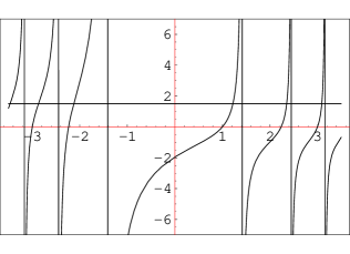
FIG. 1.: Graphics of $G(\lambda)$ for $m=1$ and $\alpha=1/4$. The horizontal line corresponds to a positive value of $\beta(\gamma)$.

It is evident from Figure 1. that the spectrum of $\overline{H_{[\kappa]}^{\gamma}}$ does depend on $\gamma$. If $\gamma_{0}<\gamma<\pi$, the eigenvalues lie between a zero of $G(\lambda)$ and the nearest pole on its right: For $\lambda>m$

$$\sqrt{m^{2}+4(N+1)}<\lambda_{N}<\sqrt{m^{2}+4(\alpha+N+1)},$$ (40)

with $N=0,1,2,\ldots$ and, for $\lambda<m$,

$$-\sqrt{m^{2}-4N}<\lambda_{N}<-\sqrt{m^{2}+4(\alpha-N-1)},$$ (41)

with $N=-1,-2,-3,\ldots$

For $-\pi<\gamma<\gamma_{0}$ the eigenvalues are bounded on the left by a pole and on the right by the nearest zero of $G(\lambda)$: For $\lambda>m$

$$\sqrt{m^{2}+4(\alpha+N-1)}<\lambda_{N}<\sqrt{m^{2}+4N},$$ (42)

with $N=1,2,3,\ldots$,

$$-\sqrt{m^{2}+4\alpha}<\lambda_{0}<m,$$ (43)

and, for $\lambda<0$,

$$-\sqrt{m^{2}+4(\alpha-N)}<\lambda_{N}<-\sqrt{m^{2}-4N}$$ (44)

with $N=-1,-2,-3,\ldots$

Notice that there is only one level with $|\lambda|<\sqrt{m^{2}+4\alpha}$. Moreover, the spectrum of $\overline{H_{[\kappa]}^{\gamma}}$ is symmetric with respect to the origin only for $\gamma=\pi$ and (except for the eigenvalue $\lambda_{0}=m$) for $\gamma=\gamma_{0}$.

V Spectrum of $\overline{H_{l}}$ for $l\neq[\kappa]$

In this section we complete the description of the Hamiltonian spectrum by computing the eigenfunctions and eigenvalues of $\overline{H_{l}}$ for $l\neq[\kappa]$.

As we saw in Section III, in the present case $H_{l}$ is essentially self-adjoint, admitting a unique self-adjoint extension given by the closure of its graph. According to Appendix B, the vectors in ${\cal D}(\overline{H_{l}})$ are absolutely continuous functions vanishing at the origin.

We are looking for solutions of the system given by eqs. (29-30) in this domain. Once again, by an argument similar to the one employed in Section III, one can see that the eigenvectors belong to ${\cal C}^{\infty}\bigcap L_{2}(\textbf{R}^{+},2\pi x\,dx)$.

Following the same steps as in Section IV, one obtains the solutions in terms of Kummer’s functions. It is convenient to write them in terms of the following pair of linearly independent solutions of eq. (17):

$$F_{1}(x^{2})=M(a;b;x^{2}),$$ (45)

$$F_{2}(x^{2})=x^{2\alpha}M(1+a-b;2-b;x^{2}),$$ (46)

where $a=\frac{m^{2}-\lambda^{2}}{4}$ and $b=1-\alpha$, with $\alpha=\kappa-l$ ($\notin\textbf{Z}$ - see footnote † ‣ III -). We will consider the cases $l<[\kappa]$ and $l>[\kappa]$ separately.

$l<[\kappa]$

For $l<[\kappa]$ ($\alpha=\kappa-l>1$), only $F_{2}(x^{2})$ leads to functions

$$\phi_{\lambda}=e^{-x^{2}/2}x^{\alpha}M(\frac{m^{2}-\lambda^{2}}{4}+\alpha;1+\alpha;x^{2}),$$ (47)

$$\chi_{\lambda}=\left[\frac{2i}{(m+\lambda)}\right]e^{-x^{2}/2}x^{-1+\alpha}\times$$ (48)

$$\left[\alpha M(\frac{m^{2}-\lambda^{2}}{4}+\alpha;1+\alpha;x^{2})+\right.$$ (49)

$$\left.\frac{m^{2}-\lambda^{2}+4\alpha}{4(1+\alpha)}x^{2}M(\frac{m^{2}-\lambda^{2}}{4}+\alpha+1;2+\alpha;x^{2})\right],$$ (50)

which are in $L_{2}((0,\delta>0),2\pi x\,dx)$. Moreover, the condition $\phi_{\lambda},\chi_{\lambda}\in L_{2}((\delta,\infty),2\pi x\,dx)$ requires that $M(1+a-b;2-b;x^{2})$ reduces to a polynomial, which occurs only when

$$1+a-b=\kappa-l+\frac{m^{2}-\lambda^{2}}{4}=-n,$$ (51)

with $n=0,1,2,\ldots$  So, the eigenvalues are given by

$$\lambda=\pm\,2\sqrt{m^{2}/4+\kappa+N},\ N=-l,-l+1,-l+2,\ldots$$ (52)

Notice that both, the eigenfunctions and eigenvalues depend on the singular flux $\kappa$.

$l>[\kappa]$

For $l>[\kappa]$ ($\alpha=\kappa-l<0$), only $F_{1}(x^{2})$ leads to functions

$$\phi_{\lambda}=e^{-x^{2}/2}x^{-\alpha}M(\frac{m^{2}-\lambda^{2}}{4};1-\alpha;x^{2}),$$ (53)

$$\chi_{\lambda}=\left[\frac{i(m-\lambda)}{2(1-\alpha)}\right]e^{-x^{2}/2}x^{1-\alpha}\times$$ (54)

$$M(\frac{m^{2}-\lambda^{2}}{4}+1;2-\alpha;x^{2}),$$ (55)

which are in $L_{2}((0,\delta>0),2\pi x\,dx)$. Once again, the condition $\phi_{\lambda},\chi_{\lambda}\in L_{2}((\delta,\infty),2\pi x\,dx)$ requires that $M(a;b;x^{2})$ reduces to a polynomial, which now occurs when

$$a=\frac{m^{2}-\lambda^{2}}{4}=-n,$$ (56)

with $n=0,1,2,\ldots$  This time, the eigenvalues are given by

$$\lambda=\pm\,2\sqrt{m^{2}/4+N},\ N=0,1,2,\ldots$$ (57)

In the present case the eigenfunctions do depend on the singular flux, but the eigenvalues are independent of $\kappa$.

Finally, notice that in both cases ($l<[\kappa]$ and $l>[\kappa]$) the eigenfunctions obtained vanish at the origin, thus belonging to the domains ${\cal D}(\overline{H_{l}})$ of the corresponding operator.

A Self-adjoint extensions of unbounded operators

In this Appendix we briefly review the theory of deficiency indices of von Neumann (for an extended presentation of the subject, see Ref. [1]). We first recall the definition of the adjoint of a given linear operator.

Let $A$ be a linear operator defined on a dense subspace ${\cal D}(A)$ of a Hilbert space $H$. The domain of definition of the adjoint operator $A^{\dagger}$, ${\cal D}(A^{\dagger})$, is the set of vectors $\psi\in H$ making the inner product $(\psi,A\phi)$ continuous in $\phi\in{\cal D}(A)$. In virtue of the Riesz - Fischer theorem, for any such $\psi$ there exists a unique vector $\chi\in H$ satisfying $(\psi,A\phi)=(\chi,\phi),\ \forall\phi\in{\cal D}(A)$. One defines $A^{\dagger}\psi\equiv\chi$.

A linear operator $A$ is symmetric if

$$\left(\phi_{1},A\,\phi_{2}\right)=\left(A\,\phi_{1},\phi_{2}\right),\forall\phi_{1},\phi_{2}\in{\cal D}(A).$$ (A1)

A linear operator $A$ is self-adjoint if it coincides with its adjoint $A^{\dagger}$, i.e. if ${\cal D}(A^{\dagger})={\cal D}(A)$ and

$$A^{\dagger}\phi=A\phi,\forall\phi\in{\cal D}(A).$$ (A2)

To establish the conditions a closed symmetric operator must satisfy to be self-adjoint, a few definitions are in order. Let ${\cal K}_{\pm}=Ker(A^{\dagger}\mp i)$ be the characteristic subspaces of $A^{\dagger}$ corresponding to the $\pm i$ eigenvalues respectively. The deficiency indices of the operator $A$, $n_{\pm}$, are defined as the dimensions of the subspaces ${\cal K}_{\pm}$.

It is worth recalling that a closed symmetric operator is self-adjoint if and only if its deficiency indices are zero [1]. However, if the deficiency indices are not zero but equal the operator admits a family of self-adjoint extensions whose construction can be carried out by means of the following theorem [1]: Let $A$ be a closed symmetric operator whose deficiency indices $n_{\pm}$ are equal; then it admits a family of self-adjoint extensions which are in a one-to-one correspondence with the unitary maps from ${\cal K}_{+}$ onto ${\cal K}_{-}$.

In fact, let ${\cal U}$ be such an isometry, then the corresponding self-adjoint extension $A_{\cal U}$ has domain ${\cal D}(A_{\cal U})=\{\psi:\psi=\phi+\phi_{+}+{\cal U}(\phi_{+})\}$, where $\phi\in{\cal D}(A)$, and $\phi_{+}\in{\cal K}_{+}$. The action of the extension $A_{\cal U}$ is given by

$$A_{\cal U}(\phi+\phi_{+}+{\cal U}(\phi_{+}))=A(\phi)+i\phi_{+}-i{\cal U}(\phi_{+}).$$ (A3)

This provides a method for constructing the self-adjoint extensions of closed symmetric operators with equal deficiency indices by identifying each possible unitary map from ${\cal K}_{+}$ onto ${\cal K}_{-}$.

B Closure of ${H_{l}}$

In this appendix we will study the closure $\overline{H_{l}}$ of the operator in eq. (6),

$$H_{l}=\left(\begin{array}[]{cc}m&i\left(\frac{d}{dx}+\frac{1-\alpha}{x}-x\right)\\ i\left(\frac{d}{dx}+\frac{\alpha}{x}+x\right)&-m\end{array}\right),$$ (B1)

defined on ${\cal D}(H_{l})=C^{\infty}_{0}(\textbf{R}^{+})$, a dense subspace of $L_{2}(\textbf{{R}}^{+},2\pi x\,dx)$. It will be shown that the functions in the domain of definition of $\overline{H_{l}}$ are continuous near the origin, and vanishing for $x\rightarrow 0^{+}$.

In order to obtain ${\cal D}(\overline{H_{l}})$ we must add to the domain of $H_{l}$ the limit points of the Cauchy sequences in ${\cal D}(H_{l})$ whose images by $H_{l}$ are also Cauchy sequences.

So, let us consider a Cauchy sequence $\{\psi_{n}\}_{n\in\mathbf{N}}$ with $\psi_{n}\in{\cal D}(H_{l}),\forall n\in\mathbf{N}$, and such that $\{H_{l}\psi_{n}\}_{n\in\mathbf{N}}$ is also a Cauchy sequence. Therefore, given $\varepsilon>0$,

$$\|\psi_{n}-\psi_{m}\|^{2}<\varepsilon$$ (B2)

$$\|H_{l}(\psi_{n}-\psi_{m})\|^{2}<\varepsilon$$ (B3)

for $n,m$ sufficiently large. Making use of eq. (B1), it is easily seen that

$$\|H_{l}(\psi_{n}-\psi_{m})\|^{2}=$$ (B4)

$$\int_{0}^{\infty}\left(|\phi^{\prime}|^{2}+p_{(x)}|\phi|^{2}+|\chi^{\prime}|^{2}+q_{(x)}|\chi|^{2}\right)2\pi xdx,$$ (B5)

where we have denoted by $\phi$ and $\chi$ respectively the upper and lower component of $(\psi_{n}-\psi_{m})$, while the functions $p(x),q(x)$ are given by

$$p{(x)}=\left[\left(\frac{\alpha}{x}+x\right)^{2}+m^{2}-2\right],$$ (B6)

$$q{(x)}=\left[\left(\frac{1-\alpha}{x}+x\right)^{2}+m^{2}+2\right],$$ (B7)

and are $O(x^{-2})$ for $x\rightarrow 0^{+}$ (since we are taking $\alpha\notin\textbf{Z}$ - see footnote † ‣ III -). It is not hard to see that both $p(x)$ and $q(x)$ are positive in the interval $[0,\delta]$ for some positive $\delta$. Only $p(x)$ can change its sign in an interval $(x_{1},x_{2})$ (depending on $\alpha$ and $m$), with $0<\delta<x_{1}<x_{2}<\infty$. Notice that the integrand of eq. (B4) (obtained through an integration by parts) could take negative values only in $(x_{1},x_{2})$, as a consequence of the term $p(x)|\phi(x)|^{2}$.

Moreover, for $\delta$ small enough, we can choose $K>0$ such that $p(x)>{K}/{x^{2}}$. Taking into account eqs. (B2) and (B4), for a given $\varepsilon>0$, we can write

$$\int_{0}^{\delta}|\phi^{\prime}|^{2}x\,dx<\varepsilon,\ \int_{0}^{\delta}\frac{|\phi|^{2}}{x}\,dx<\varepsilon,$$ (B8)

and

$$\int_{0}^{\delta}|\chi^{\prime}|^{2}x\,dx<\varepsilon,\ \int_{0}^{\delta}\frac{|\chi|^{2}}{x}\,dx<\varepsilon,$$ (B9)

if $n,m$ are large enough. Therefore,

$$\{\sqrt{x}\,\psi^{\prime}_{n}(x)\}\ {\rm and}\ \{\psi_{n}(x)/\sqrt{x}\}$$ (B10)

are Cauchy sequences in $L_{2}(0,\delta)$ (with respect to the usual Lebesgue measure), as well as the sum

$$\{\sqrt{x}\,\psi^{\prime}_{n}(x)+\psi_{n}(x)/(2\sqrt{x})\}=\{\left[\sqrt{x}\,\psi_{n}(x)\right]^{\prime}\}.$$ (B11)

Let us call $\Phi(x)=\lim_{n\rightarrow\infty}\left[\sqrt{x}\,\psi_{n}(x)\right]^{\prime}\in L_{2}(0,\delta)$, and denote its primitive by

$$\sqrt{x}\,\Psi(x)\equiv\int_{0}^{x}\Phi(y)\,dy,$$ (B12)

which is an absolutely continuous function [1] in $(0,\delta)$. In particular, $\Psi(x)$ is continuous in $(0,\delta)$.

On the basis of

$$|\sqrt{x}(\Psi(x)-\psi_{n}(x))|=$$ (B13)

$$\left|\int_{0}^{x}\left[\Phi(y)-(\sqrt{y}\,\psi_{n}(y))^{\prime}\right]dy\right|\leq$$ (B14)

$$\sqrt{\int_{0}^{\delta}\left|\Phi(y)-(\sqrt{y}\psi_{n}(y))^{\prime}\right|^{2}dy}\sqrt{\int_{0}^{\delta}1\,dy}$$ (B15)

$$\longrightarrow 0,\ {\rm for}\ n\rightarrow\infty,$$ (B16)

we conclude that the sequence $\{\sqrt{x}\,\psi_{n}(x)\}$ converges uniformly to $\sqrt{x}\,\Psi(x)$ in $(0,\delta)$, and consequently also in the metric of $L_{2}(0,\delta)$,

$$\lim_{n\rightarrow\infty}\left\{\sqrt{x}\,\psi_{n}(x)\right\}=\sqrt{x}\,\Psi(x).$$ (B17)

(Notice that $\Psi(x)$ is the limit of $\{\psi_{n}(x)\}$ in $L_{2}[(0,\delta),x\,dx]$.)

In addition, it is straightforward to show that

$$\frac{\Psi(x)}{\sqrt{x}}=\lim_{n\rightarrow\infty}\left\{\frac{\psi_{n}(x)}{\sqrt{x}}\right\}.$$ (B18)

Then, we conclude from eqs. (B18) and (B12) that

$$\lim_{n\rightarrow\infty}\left\{\sqrt{x}\psi^{\prime}_{n}(x)\right\}=\sqrt{x}\Psi^{\prime}(x),$$ (B19)

in the metric of $L_{2}(0,\delta)$.

Therefore, we can write

$$\int_{0}^{\delta}|\Psi^{\prime}|^{2}x\,dx<\infty,\ \int_{0}^{\delta}\frac{|\Psi|^{2}}{x}\,dx<\infty.$$ (B20)

This implies that $\Psi^{\prime}(x)\cdot\Psi(x)=1/2\left(\Psi(x)\cdot\Psi(x)\right)^{\prime}\in L_{1}(0,\delta)$.

On the other hand, the components of $\Psi(x)$, $\Psi_{\alpha}(x)$ with $\alpha=1,2$, are absolutely continuous functions in $(\epsilon,\delta)$, for $\epsilon<\delta$, by virtue of eq. (B12). In consequence

$$\int_{\epsilon}^{\delta}\left(\Psi_{\alpha}^{2}(x)\right)^{\prime}\,dx=\Psi_{\alpha}^{2}(\delta)-\Psi_{\alpha}^{2}(\epsilon).$$ (B21)

In this expression we can take the $\lim_{\epsilon\rightarrow 0^{+}}$, proving that the continuous function $\Psi_{\alpha}^{2}(x)$ has a well defined limit for $x\rightarrow 0^{+}$. Moreover, on account of eq. (B20), this limit must be zero.

As a consequence of the previous results, we conclude that the behavior near the origin of the functions in ${\cal D}(\overline{H_{[\kappa]}^{\gamma}})$ is dominated by the functions in ${\cal K}_{\pm}$ (see eqs. (24-25)).

On the other hand, since the restriction of the Hamiltonian to the subspaces with $l\neq[\kappa]$ is, as already mentioned, essentially self-adjoint, the behavior of the functions at the origin is dictated by its closure, therefore being continuous and satisfying the boundary condition

$$\lim_{x\rightarrow 0^{+}}\psi(x)=0.$$ (B22)

Acknowledgements: The authors thank M.A. Muschietti and E.M. Santangelo for useful discussions and comments. H. F. thanks P. Giacconi and R. Soldati for calling his attention to this problem. This work was partially supported by ANPCyT (PICT’97 Nr. 00039), and CONICET (PIP Nr. 0459) of Argentina.

REFERENCES

• [1] Methods of Modern Mathematical Physics, Vol. I - II. M. Reed and B. Simon. Academic Press, New York (1980).
• [2] Y. Aharonov and D. Bohm, Phys. Rev. 115, 485 (1959).
• [3] Ph. de Sousa Gerbert, Phys. Rev. D 40, 1346 (1989).
• [4] R. Adami and A. Teta, Lett. Math. Phys. 43, 43 (1998).
• [5] Yu. A. Sitenko, Physics of Atomic Nuclei Vol.62, 1084 (1999).
• [6] Yu. A. Sitenko, Annals of Physics 282, 167 (2000).
• [7] C. R. Hagen, Phys. Rev. Lett. 64, 503 (1990).
• [8] M. G. Alford, J. March-Russell and F. Wilczek, Nucl. Phys. B328, 140 (1989).
• [9] H. P. Thienel, Annals of Physics 280, 140-162 (2000).
• [10] R. M. Cavalcanti, Comment on ”Quantum mechanics of an electron in a homogeneous magnetic field and a singular magnetic flux tube”, (2000) quant-ph/0003148.
• [11] Alexios P. Polychronakos, Nucl. Phys. B278, 207 (1986); Nucl. Phys. B283, 268 (1987).
• [12] C. G. Beneventano, M. De Francia and E. M. Santangelo, Int. Journ. of Mod. Phys. A, Vol. 14, No. 30, 4749 (1999).
• [13] F. Bentosela, R.M. Cavalcanti, P. Exner, V.A. Zagrebnov, J. Phys. A32, 3029 (1999).
• [14] M. Bordag and S. Voropaev, J. Phys. A26, 7637 (1993).
• [15] R.M. Cavalcanti, C.A.A. de Carvalho, J. Phys. A31, 7061 (1998).
• [16] R.M. Cavalcanti, E.S. Fraga and C.A.A. de Carvalho, Phys. Rev. B56, 9243 (1997).
• [17] A. Moroz, Phys. Rev. A53, 669 (1996).
• [18] E. G. Flekkøy and J. M. Leinaas, Int. Journ. of Mod. Phys. A 6, 5327 (1991).
• [19] J. Desbois, S. Ouvry and C. Teixer, Nucl. Phys. B 500, 486 (1997).
• [20] P. Giacconi and R. Soldati, J.  Phys. A33, 5193 (2000).
• [21] M. Franz and Z. Tešanović, Phys. Rev. Lett. 84, 554 (2000).
• [22] O. Vafek, A. Melikyan, M. Franz and Z. Tešanović, ”Quasiparticles and Vortices in Unconventional Superconductors”, cond-mat/0007296 (2000).
• [23] Handbook of Mathematical Functions. M. Abramowitz and I. Stegun editors. Dover Publications, New York (1970).