Fredholm Indices and the Phase Diagram of Quantum Hall Systems

Abstract

The quantized Hall conductance in a plateau is related to the index of a Fredholm operator. In this paper we describe the generic “phase diagram” of Fredholm indices associated with bounded and Toeplitz operators. We discuss the possible relevance of our results to the phase diagram of disordered integer quantum Hall systems.

PACS: 73.40.Hm, also 71.10Hf, 03.65.Db

The Hall conductance of Integer Quantum Hall systems is described mathematically by the index of Fredholm operators. (For precise definitions, see below). In this paper we investigate the phase diagram of the Fredholm index for a few classes of operators. For the algebra of bounded operators, little can be said beyond the fact that the phase diagrams can be arbitrarily complicated. But for the algebra of Toeplitz operators, and other related classes of operators, we establish a kind of a Gibbs phase rule [1]. Typical of our results is the statement that if the system is governed by two parameters, then one should expect jumps by one at phase boundaries and jumps by up to 2 at triple points, while jumps by more than two should never be observed.

We relate this behavior to experimental results, conjectures and open problems that arise in the context of the Quantum Hall Effect (QHE) [2].

In Section 1 we define Fredholm operators and their indices, and explore the different sorts of phase diagrams that can arise. In Section 2 we recall how Fredholm indices are related to the conductance of Quantum Hall systems. In Section 3 we consider phase diagrams for general bounded operators. In Section 4 we describe the phase diagram for linear combination of shift operators, and in Section 5 we consider general Toeplitz operators. In Section 6 we discuss the phase diagrams of soluble models related to the quantum Hall effect, and how they might be modified by disorder. We also discuss the relevance of Toeplitz operators to the Quantum Hall Effect and present some open problems.

I Fredholm indices

I.1 Basic notions

The following is a brief description of Fredholm operators. For more details, see [3, 4, 5].

Definition 1

A bounded operator $F$ on a separable Hilbert space is Fredholm if there exists a bounded operator $B$ such that $1-FB$ and $1-BF$ are compact. The Fredholm index is defined by

$$Index(F)=dim\,Ker(F)-dim\,Ker(F^{\dagger}).$$ (1)

The simplest example of a Fredholm operator with nonzero index is the unilateral shift operator: Let $e_{0},e_{1},e_{2},\ldots$ be the canonical basis for the Hilbert space $\ell^{2}(\mathbb{N})$, and let the operator $a$ act by

$$a(e_{n})=\begin{cases}e_{n-1}&if\ n>0\cr 0&if\ n=0.\end{cases}$$ (2)

The reason for denoting the unilateral shift operator by $a$ is its similarity to the harmonic oscillator lowering operator. The adjoint of $a$ acts by

$$a^{\dagger}(e_{n})=e_{n+1}$$ (3)

Since ${1}=aa^{\dagger}=a^{\dagger}a+|e_{0}\rangle\langle e_{0}|$, $a$ is Fredholm. The kernel of $a$ is 1-dimensional and the kernel of $a^{\dagger}$ is 0-dimensional. Thus $Index\ (a)=1$ and $Index\ (a^{\dagger})=-1$.

Although neither the dimension of $Ker\ F$ nor that of $Ker\,F^{\dagger}$ is stable under deformations of $F$, the index is stable. For any compact operator $C$, for any bounded operator $B$, and for $\epsilon$ sufficiently small, [4, 5]:

$$Index(F)=Index(F+\epsilon B+C).$$ (4)

The following theorem is standard:

Theorem 1

If $A_{1},\ldots A_{n}$ are Fredholm operators, then the product $A_{1}A_{2}\cdots A_{n}$ is also Fredholm, and $Index(A_{1}\cdots A_{n})=\sum_{i=1}^{n}Index(A_{i})$.

If $F$ and $F^{\prime}$ are Fredholm operators on the same Hilbert space, then there is a continuous path of Fredholm operators from $F$ to $F^{\prime}$ if and only if $Index(F)=Index(F^{\prime})$. (By continuous, we mean relative to the operator norm). Put another way, the path components of $Fred(H)$, the space of Fredholm operators on $H$, are indexed by the integers. The $n$-th path component is precisely the set of Fredholm operators of index $n$ [4].

I.2 Phase diagrams

Our main concern in this paper is the following problem: Suppose one interpolates between Fredholm operators with different indices. What can one say about the way the indices change? Another way of phrasing this is: What is the phase diagram of Fredholm indices?

The answer to this question depends on the choice of the embedding space. In the space of bounded operators, the “phases”—each labeled by its index—are open sets. But the boundary between phases, as we shall explain, is rather wild: A point on the boundary of one phase is also on the boundary of every other phase. This behavior is difficult to visualize.

Another class of embedding spaces that we consider is associated with Toeplitz operators with various regularity assumptions on a class of functions. Here, at least if the functions are sufficiently smooth, the boundaries between phases have a simple structure and the phase diagrams satisfy simple rules that have the flavor of Gibbs’ phase rule [1]. Typical of our results is the statement that under appropriate conditions, phases whose indices differ by one have a common boundary whose codimension is one, and phases whose indices differ by two meet on a set of codimension two etc. Fig. 1 is an example of one of the phase diagrams we obtain.

II The Hall conductance as a Fredholm Index

Theories of the quantum Hall effect are roughly of two kinds: those that focus on the bulk of the Hall and those that focus on the edge [2]. It was pointed out by [6] that the bulk-edge duality is an illustration of the holographic principle. In either approach, the quantized Hall conductance can be related to a Fredholm index.

II.1 Theories of the bulk

It is common knowledge that the Hall conductance can be identified with a Chern number [7]. For non-interacting electrons in two dimensions, this result is a special case of the fact that the Hall conductance is a Fredholm index. Since this is not common knowledge, we recall how Chern numbers and Fredholm indices are related.

For non-interacting electrons in two dimensions with the Fermi energy in a gap, TKN², showed that the Hall conductance for Landau Hamiltonians with periodic potential, is related to a Chern number [8]. The (magnetic) Brillouin zone associated with the periodicity plays an role in this theory. Because of this, the interpretation of the Hall conductance as a Chern number does not carry over to random or even quasi-periodic potentials nor to “irrational magnetic fields”, all of which have no (classical) Brillouin zone. Although the quantization of the Hall conductance can be established in these cases by a limiting argument [9, 7], the interpretation as a Chern number does not survive.

J. Bellissard [10], in a work that had impact on non-commutative geometry [11, 12], showed that the Hall conductance with ergodic potential, be it periodic, quasi-periodic or random, and real magnetic field, rational or not, is a Fredholm index. This result was derived in [13] without using non-commutative geometry.

More precisely, consider the (infinite dimensional) spectral projection $P$ on the states below the Fermi energy $E_{F}$ for the one particle Hamiltonian in the plane. Let $U$ be the multiplication operator $e^{i\theta}$, where $\theta$ is the usual polar angle in the plane. $U$ is a singular gauge transformation that introduces an Aharonov-Bohm flux tube at the origin of the Euclidean plane. The Hall conductance is the Fredholm index of $PUP$ thought of as an operator on the range of $P$ [14]. Since the Fredholm index does not need a Brillouin zone, this approach offers a natural framework that accounts for the quantization and stability of the Hall conductance.

II.2 Theories of the edge

Finite quantum Hall systems have chiral edge currents [15, 16]. Consider the case that the boundary is a circle of circumference $L$. The dispersion relation of the edge states is approximately linear in a small neighborhood of the Fermi energy and the Hamiltonian for a single edge channel, with velocity $v_{F}$, is

$$H=-i\frac{v_{F}}{L}\partial_{\theta}$$ (5)

Now, the projection $P$ is associated with the occupied edge states, $e^{-im\theta}$ with $m\geq m_{0}$. Introducing a flux tube into the system is associated with the unitary $U=e^{i\theta}$ and sends $H\to UHU^{\dagger}$. This leads to the spectral flow of the edge states. $PUP$ is the unilateral shift operator $a$ and the number of edge states that cross the Fermi energy is $Index\,PUP=1$. By an argument of Halperin [15] this is also the Hall conductance.

An extension of this idea to Harper models with an edge is described in [17].

III The phase diagram for bounded operators

We begin with the space of bounded operators with the topology defined by the operator norm, and we wish to understand the phase diagram of a generic family of such operators. As we shall explain, the phase diagram in the entire space is quite wild: Any point on the boundary of the “index = $k$” phase is also on the boundary of every other phase.

To understand this bizarre behavior, recall that the zero operator (which is not a Fredholm operator) is on the boundary of every phase: Zero is the limit, as $\varepsilon\to 0$, of $\varepsilon a^{n}$, with $a$ of Eq. (2), for any $n$. The point of the theorem is that similar behavior occurs at all boundary points.

Theorem 2

Let $U_{n}$ be the set of Fredholm operators of index $n$. Every point on the boundary of $U_{n}$ is also on the boundary of $U_{m}$, for every integer $m$.

Proof: Let $A$ be a (not Fredholm) operator on the boundary of $U_{n}$. Given $\epsilon>0$, we must find an operator in $U_{m}$ within a distance $\epsilon$ of $A$.

Suppose that the kernel and cokernel of $A$ are infinite dimensional, and that there is a gap in the spectrum of $A^{\dagger}A$ at zero. (If this is not the case, we may perturb $A$ by an arbitrarily small amount to make it so). Now let $B$ be a unitary map from the kernel of $A$ to the cokernel. Let $P,\ (P^{\prime})$ be the orthogonal projection onto $ker(A),\ (coker(A))$, and let $a$ be a shift operator on $ker(A)$. For each $m\geq 0$, $A(\epsilon)=A+\epsilon Ba^{m}P$ has a bounded right inverse

$$A^{\dagger}{1\over P^{\prime}+AA^{\dagger}}P^{\prime}_{\perp}+{1\over\epsilon}(a^{\dagger})^{m}B^{\dagger}P^{\prime}.$$ (6)

It follows that the cokernel of $A(\epsilon)$ is empty. It is easy to see that the kernel of $A(\epsilon)$ is $m$ dimensional hence $Index(A(\epsilon))=m$. Similarly, $A+\epsilon B(a^{\dagger})^{m}P$ has index $-m$.     

IV Linear combinations of shifts

In this section and the next we show that there are interesting and simple “generic” phase diagrams of Fredholm indices in some finite dimensional spaces, and in some infinite-dimensional spaces with sufficiently fine topologies. We shall also see also how control is lost as the space is enlarged and the topology is coarsened.

IV.1 Shift by one

We begin by considering linear combinations of the shift operator $a$ and the identity operator 1. That is, we consider the operator

$$A=c_{1}a+c_{0}$$

where $c_{1}$ and $c_{0}$ are constants.

Theorem 3

If $|c_{1}|\neq|c_{0}|$, then $A$ is Fredholm. The index of $A$ is 1 if $|c_{1}|>|c_{0}|$ and zero if $|c_{1}|<|c_{0}|$. If $|c_{1}|=|c_{0}|$, then $A$ is not Fredholm.

Proof: First suppose $|c_{0}|>|c_{1}|$. Then $A$ is invertible:

$$A^{-1}=c_{0}^{-1}(1+(c_{1}/c_{0})a)^{-1}=\sum_{n=0}^{\infty}{(-1)^{n}c_{1}^{n}\over c_{0}^{n+1}}a^{n},$$

as the sum converges absolutely. Thus $A$ has neither kernel nor cokernel, and has index zero.

If $|c_{1}|>|c_{0}|$, then the kernel of $A$ is 1-dimensional, namely all multiples of $|\psi\rangle=\sum_{n=0}^{\infty}z_{0}^{n}e_{n}$, where $z_{0}=-c_{0}/c_{1}$. Notice how the norm of $|\psi\rangle$ goes to infinity as $|z_{0}|\to 1$. However, $A^{\dagger}$ has no kernel, since for any unit vector $|\phi\rangle$, $\|A^{\dagger}|\phi\rangle\|=\|\bar{c}_{1}a^{\dagger}|\phi\rangle+\bar{c}_{0}|\phi\rangle\|\geq\|\bar{c}_{1}a^{\dagger}|\phi\rangle\|-\|\bar{c}_{0}|\phi\rangle\|=|c_{1}|-|c_{0}|$. Thus the index of $A$ is 1.

If $|c_{1}|=|c_{0}|$, then $A$ is at the boundary between index 1 and index 0, and so cannot be Fredholm.     

IV.2 Finite linear combinations of shifts

Next we consider linear combinations of $1,a,a^{2},\ldots$ up to some fixed $a^{n}$. That is, we consider operators of the form

$$A=c_{n}a^{n}+c_{n-1}a^{n-1}+\cdots+c_{0}.$$ (7)

This is closely related to the polynomial

$$p(z)=c_{n}z^{n}+\cdots+c_{0}.$$ (8)

Theorem 4

If none of the roots of $p$ lie on the unit circle, then $A$ is Fredholm, and the index of $A$ equals the number of roots of $p$ inside the unit circle, counted with multiplicity. If any of the roots of $p$ lie on the unit circle, then $A$ is not Fredholm.

Proof: The polynomial $p(z)$ factorizes as $p(z)=c_{k}\prod_{i=1}^{k}(z-\zeta_{i})$, where $k$ is the degree of $p$ (typically $k=n$, but it may happen that $c_{n}=0$). But then $A=c_{k}\prod_{i=1}^{k}(a-\zeta_{i})$. If none of the roots $\zeta_{i}$ lie on the unit circle, then each term in the product is Fredholm, so the product is Fredholm, and the index of the product is the sum of the indices of the factors. By Theorem 3, this exactly equals the number of roots $\zeta_{i}$ inside the unit circle.

If any of the roots lie on the unit circle, then a small perturbation can push those roots in or out, yielding Fredholm operators with different indices. This borderline operator therefore cannot be Fredholm.     

The last theorem easily generalizes to linear combination of left-shifts and right-shifts. The index of an operator

$$A=c_{n}a^{n}+\cdots+c_{1}a+c_{0}+c_{-1}a^{\dagger}+\cdots+c_{-m}(a^{\dagger})^{m}$$ (9)

equals the number of roots of

$$p(z)=\sum_{i=-m}^{n}c_{i}z^{i}$$ (10)

inside the unit circle, minus the degree of the pole at $z=0$ (that is $m$, unless $c_{-m}=0$). This follow from the fact that

$$A=(\sum_{i=-m}^{n}c_{i}a^{i+m})(a^{\dagger})^{m}.$$ (11)

Since there is no qualitative difference between combinations of left-shifts and combinations of both left- and right-shifts, we restrict our attention to left-shifts only, and consider families of operators of the form (7).

Theorem 5

In the space of complex linear combinations of 1, $a$, …, $a^{n}$, almost every operator is Fredholm. For every $k\leq n$, the points where the index can jump by $k$ (by which we mean the common boundaries of regions of Fredholm operators whose indices differ by $k$) is a set of real codimension $k$.

In the space of real linear combinations of 1, $a$, …, $a^{n}$, almost every operator is Fredholm. For every $k\leq n$, the points where the index jumps by $k$ is a stratified space, the largest stratum of which has real codimension $\lfloor(k+1)/2\rfloor$, where $\lfloor x\rfloor$ denotes the integer part of $x$.

Proof: Our parameter space is the space of coefficients $c_{i}$, or equivalently the space of polynomials of degree $\leq n$. This is either ${\rm I\kern-1.99997ptR}^{n+1}$ or $\kern 1.00006pt{\raise 2.0236pt\hbox{ $\scriptscriptstyle|$}}\kern-3.99994pt{\rm C}^{n+1}$, depending on whether we allow real or complex coefficients. In either case, the set $U_{k}$ of Fredholm operators of index $k$ is identical to the set of polynomials with $k$ roots inside the unit circle and the remaining $n-k$ roots outside (if $c_{n}=0$, we say there is a root at infinity; if $c_{n}=c_{n-1}=0$, there is a double root at infinity, and so on. Counting these roots at infinity, there are always exactly $n$ roots in all.) The boundary of $U_{k}$ is the set of polynomials with at most $k$ roots inside the unit circle, at most $n-k$ outside the unit circle, and at least one root on the unit circle. (Strictly speaking, the zero polynomial is also on this boundary. This is of such high codimension that it has no effect on the phase portrait we are developing.). We consider the common boundary of $U_{k}$ and $U_{k^{\prime}}$. If $k<k^{\prime}$, a nonvanishing polynomial is on the boundary of both $U_{k}$ and $U_{k^{\prime}}$ if it has at most $k$ roots inside the unit circle and at most $n-k^{\prime}$ roots outside. It must therefore have at least $k^{\prime}-k$ roots on the unit circle.

If we are working with complex coefficients, this is a set of codimension $k^{\prime}-k$. The roots themselves, together with an overall scale $c_{n}$, can be used to parametrize the space of polynomials. For each root, being on the unit circle is codimension 1, while being inside or outside are open conditions. Since the roots are independent, placing $k^{\prime}-k$ roots on the unit circle is codimension $k^{\prime}-k$.

If we are working with real coefficients, the roots are not independent, as non-real roots come in complex conjugate pairs. Thus, the common boundary of $U_{k}$ and $U_{k^{\prime}}$ breaks into several strata, depending on how many real roots and how many complex conjugate pairs lie on the unit circle. If $k^{\prime}-k$ is even, the biggest stratum consists of having $(k^{\prime}-k)/2$ pairs, and has codimension $(k^{\prime}-k)/2$. If $k^{\prime}-k$ is odd, the biggest stratum consists of having $(k^{\prime}-k-1)/2$ pairs and one real root on the unit circle, and has codimension $(k^{\prime}+1-k)/2$.    

Figure 1: A phase diagram for the Fredholm index of $F=a^{2}+c_{1}a+c_{0}$.

Theorem 5 is illustrated in Figure 1, where the phase portrait is shown for $n=2$ with real coefficients, with $c_{2}$ fixed to equal 1. The points above the parabola $c_{0}=c_{1}^{2}/4$ have complex conjugate roots, while points below have real roots. Notice that the transition from index 2 to index 0 occurs at an isolated point when the roots are real, but on an interval when the roots come in complex-conjugate pairs.

It is clear that an almost identical theorem applies to linear combinations of left-shifts up to $a^{n}$ and right-shifts up to $(a^{\dagger})^{m}$. The results are essentially independent of $n$ and $m$ (their only effect being to limit the size of possible jumps to $n+m$). We can therefore extend the results to the space of all (finite) linear combinations of left- and right-shifts, which is topologized as the union over all $n$ and $m$ of the spaces considered above. Our result, restated for that space, is

Theorem 6

In the space of finite complex linear combinations of left- and right-shifts of arbitrary degree, almost every operator is Fredholm. For every integer $k\geq 1$, the points where the index can jump by $k$ (by which we mean the common boundaries of regions of Fredholm operators whose indices differ by $k$) is a set of real codimension $k$.

If we restrict the coefficients to be real, then, for every $k\leq n$, the points where the index jumps by $k$ is a stratified space, the largest stratum of which has real codimension $\lfloor(k+1)/2\rfloor$.

V Toeplitz operators

Although Theorem 6 refers to an infinite-dimensional space, this space is still extremely small – each point is a finite linear combination of shifts. In this section we consider infinite linear combinations of shifts. This is equivalent to studying Toeplitz operators.

Definition 2

The Hardy space $H$ is the subspace of $L^{2}(S^{1})$ consisting of functions whose Fourier transforms have no negative frequency terms. Equivalently, if we give $L^{2}(S^{1})$ a basis of Fourier modes $e_{n}=e^{in\theta}$, where the integer $n$ ranges from $-\infty$ to $\infty$, then $H$ is the closed linear span of $e_{0},e_{1},e_{2},\ldots$.

We think of $S^{1}$ as sitting in the complex plane, with $z=e^{i\theta}$. Now let $f(z)$ be a bounded, measurable function on $S^{1}$, and let $P$ be the orthogonal projection from $L^{2}(S^{1})$ to $H$. If $|\psi\rangle\in H$, then $|f\psi\rangle$ (pointwise product) is in $L^{2}(S^{1})$, and $P|f\psi\rangle\in H$. We define the operator $T_{f}$ by

$$T_{f}|\psi\rangle=P|f\psi\rangle.$$ (12)

Definition 3

An operator of the form (12) is called a Toeplitz operator. We call a Toeplitz operator $T_{f}$ continuous if the underlying function $f$ is continuous, and apply the terms “differentiable”, “smooth” and “analytic” similarly.

Remark: Toeplitz operators can be represented by semi-infinite matrices that have constant entries on diagonals, and the various classes we have defined correspond to the decay away from the main diagonal.

Notice that

$$T_{e_{m}}e_{n}=\begin{cases}e_{n+m}&if\ n+m\geq 0\cr 0&otherwise\end{cases}$$ (13)

so $T_{e_{m}}$ is simply a shift by $m$, a right shift if $m>0$ and a left-shift if $m<0$. All our results about shifts can therefore be understood in the context of Toeplitz operators. Theorem 5 refers to operators $T_{f}$, where $f$ is a polynomial in $z^{-1}$ of limited degree. Theorem 6 considers polynomials or arbitrary degree in $z$ and $z^{-1}$. We will see that the results carry over to analytic functions on an annulus around $S^{1}$, and to a lesser extent to $C^{k}$ Toeplitz operators, but with results that weaken as $k$ is decreased.

Here are some standard results about Toeplitz operators. For details, see [4].

Theorem 7

A $C^{1}$ Toeplitz operator $T_{f}$ is Fredholm if and only if $f$ is everywhere nonzero on the unit circle. In that case the index of $T_{f}$ is minus the winding number of $f$ around the origin, namely

$$Index(T_{f})=-Winding(f)={-1\over 2\pi i}\int_{S^{1}}{df\over f},$$ (14)

Given the first half of the theorem, the equality of index and winding number is easy to understand. We simply deform $f$ to a function of the form $f(z)=z^{n}$, while keeping $f$ nonzero on all of $S^{1}$ throughout the deformation (this is always possible, see e.g. [18]). In the process of deformation, neither the index of $T_{f}$ nor the winding number of $f$ can change, as they are topological invariants. Since the winding number of $z^{n}$ is $n$, and since $T_{z^{n}}=(a^{\dagger})^{n}$ (if $n\geq 0$, $a^{-n}$ otherwise), which has index $-n$, the result follows.

We now consider functions $f$ on $S^{1}$ that can be analytically continued (without singularities) to an annulus $r_{0}\leq|z|\leq r_{1}$, where the radii $r_{0}<1$ and $r_{1}>1$ are fixed. This is equivalent to requiring that the Fourier coefficients $\hat{f}_{n}$ decay exponentially fast, i.e. that the sum

$$\sum_{n=-\infty}^{\infty}|\hat{f}_{n}|(r_{0}^{n}+r_{1}^{n})$$ (15)

converges. For now we do not impose any reality constraints or other symmetries on the coefficients $\hat{f}_{n}$. This space of functions is a Banach space, with norm given by the sup norm on the annulus. This norm is stronger than any Sobolev norm on the circle itself.

The analysis of the corresponding Toeplitz operators is straightforward and similar to the proof of Theorem 5. Since $f$ has no poles in the annulus, we just have to keep track of the zeroes of $f$. For the index of $T_{f}$ to change, a zero of $f$ must cross the unit circle. For the index to jump from $k$ to $k^{\prime}$, $|k-k^{\prime}|$ zeroes must cross simultaneously. In the absence of symmetry, the locations of the zeroes are independent and can be freely varied, so this is a codimension-$|k-k^{\prime}|$ event.

If we impose a reality condition: $f(\bar{z})=\overline{f(z)}$, then zeroes appear only on the real axis or in complex conjugate pairs. In that case, changing the index by 2 is merely a codimension-1 event. Combining these observations we obtain

Theorem 8

In the space of Toeplitz operators that are analytic in a (fixed) annulus containing $S^{1}$, almost every operator is Fredholm. For every integer $k\geq 1$, the points where the index can jump by $k$ is a set of real codimension $k$.

If we impose a reality condition $f(\bar{z})=\overline{f(z)}$ then, for every $k\leq n$, the points where the index jumps by $k$ is a stratified space, the largest stratum of which has real codimension $\lfloor(k+1)/2\rfloor$.

Finally we consider Toeplitz operators that are not necessarily analytic, but are merely $\ell$ times differentiable, and we use the $C^{\ell}$ norm. Our result is

Theorem 9

In the space of Toeplitz $C^{\ell}$ operators, almost every operator is Fredholm. For every integer $k$ with $1\leq k\leq 2\ell+1$, the points where the index can jump by $k$ is a set of real codimension $k$. For every integer $k\geq 2\ell+1$, the points where the index can jump by $k$ is a set of real codimension $2\ell+1$.

In other words, our familiar results hold up to codimension $2\ell+1$, at which point we lose all control of the change in index.

Proof: As long as $f$ is everywhere nonzero, $T_{f}$ is Fredholm. To get a change in index, therefore, we need one or more points where $f$, and possibly some derivatives of $f$ with respect to $\theta$, vanish. Suppose then that for some angle $\theta_{0}$, $f(\theta_{0})=f^{\prime}(\theta_{0})=\cdots=f^{(n-1)}(\theta_{0})=0$ for some $n\leq\ell$, but that the $n$-th derivative $f^{(n)}(\theta_{0})\neq 0$. This is a codimension $2n-1$ event, since we are setting the real and imaginary parts of $n$ variables to zero, but have a 1-parameter choice of points where this can occur. Without loss of generality, we suppose that this $n$-th derivative is real and positive. By making a $C^{\ell}$-small perturbation of $f$, we can make the value of $f$ highly oscillatory near $\theta_{0}$, thereby wrapping around the origin a number of times. However, since a $C^{\ell}$-small perturbation does not change the $n$-th derivative by much, the sign of the real part of $f$ can change at most $n$ times near $\theta_{0}$, so the argument of $f$ can only increase or decrease by $n\pi$ or less. The difference between these two extremes is $2n\pi$, or a change in winding number of $n$.

To change the index by an integer $m$, therefore, we must have the function vanish to various orders at several points, with the sum of the orders of vanishing adding to $m$. The generic event is for $f$ (but not $f^{\prime}$) to vanish at $m$ different points – this is a codimension $m$ event, analogous to having $m$ zeroes of a polynomial cross the unit circle simultaneously at $m$ different points. All other scenarios have higher codimension and are analogous to having 2 or more zeroes of the $m$ zeroes crossing the unit circle at the same point.

The situation is different, however, when the function $f$ and the first $\ell$ derivatives all vanish at a point $\theta_{0}$. Then the higher-order derivatives are not protected from $C^{\ell}$-small perturbations and, by making such a perturbation, we can change $f$ into a function that is identically zero on a small neighborhood of $\theta=\theta_{0}$. By making a further small perturbation, we can make $f$ wrap around the origin as many times as we like near $\theta=\theta_{0}$. More specifically, if $f$ is zero on an interval of size $\delta$, then, for small $\epsilon$, $\tilde{f}(\theta)=f(\theta)+\epsilon e^{iN\theta}$ will wrap around the origin approximately $N\delta/2\pi$ times near $\theta_{0}$. By picking $N$ as large (positive or negative) as we wish, we can obtain arbitrarily positive or negative indices. As long as we take $\epsilon\ll N^{-\ell}$, this perturbation will remain small in the $C^{\ell}$ norm.    

The results of this section can be extended, with minor modifications, to the algebra of matrix valued Toeplitz operators [4] where the index is related to the winding of the determinant of a matrix.

VI Quantum Hall systems

VI.1 Phase diagrams of soluble models

Phase diagrams of quantum Hall system describe the dependence of the Hall conductance on parameters such as the magnetic field $B$ and the Fermi energy $E$. There are three idealized models where the phase diagram can be computed explicitly: The Landau Hamiltonian in the Euclidean plane, whose phase diagram is shown in Fig. 2; The Landau Hamiltonian for the hyperbolic plane, whose phase diagram is shown in Fig. 3 and Harper models in the plane [19, 8], whose phase diagram is associated with the Hofstadter butterfly, shown in Fig. 4 for the case of a tight binding model on a square lattice.

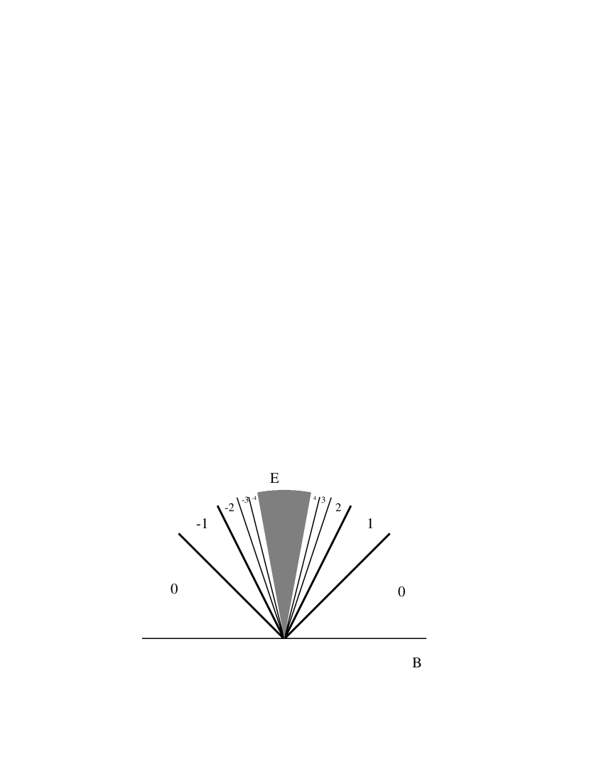
Figure 2: The phase diagram for the Landau Hamiltonian in the Euclidean plane. The shaded wedge contains infinitely many, thinner and thinner, wedges, with indices that go to $\pm\infty$ and accumulate at the $B$ axis.

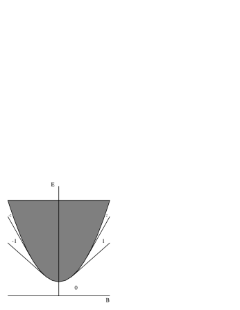
Figure 3: The phase diagram for the Landau Hamiltonian in the hyperbolic plane. In the shaded parabolic region the operator is not Fredholm and the index is nor defined.

Figure 4: The phase diagram for the Harper model associated with tight binding model on a square lattice the plane. Every point on the boundary between two phases appears to be a point of accumulation of infinitely many phases. Figure taken, with permission, from [31].

These are not models of Toeplitz operators, and none of these models is generic, especially insofar as all of them have symmetries. However, we consider the extent to which they follow the generic phase rules of (smooth, complex) Toeplitz operators anyway. Where these rules are not followed, we consider how a small generic perturbation might restore the rules.

The phase diagram for the Euclidean plane, Fig. 2 satisfies the generic phase rules away from the line $B=0$. On the line $B=0$, however, the index takes an infinitely large jump, while at the origin infinitely many phases meet. Both are forbidden by the phase rules.

The phase diagram in the hyperbolic plane, Fig. 3, satisfies the generic phase rules outside the shaded parabolic region. In the shaded region, the operator is not Fredholm and the index is not defined. This is contrary to the phase rules since not being Fredholm is expected to be a codimension 1 event.

The phase diagram of the Harper model, Fig. 4, is in serious conflict with the phase rule for (smooth, complex) Toeplitz operators: It is known [20], that for a full measure of values of the magnetic field (irrational, of course), the spectrum is a Cantor set. Since the boundary between phases is contained in the spectrum, this suggests that any point on the boundary between any two phases can also be on the boundary between infinitely many other phases. This is the sort of behavior we observed for bounded operators with no restrictions. However, even in this wildness there is some regularity. For example, the center of the figure is on the boundary of all phases with odd indices while Theorem 2 allows for even indices as well.

Remark 1

To see how Fig. 4 is obtained, we recall that for a tight-binding model with flux $\frac{p}{q}$ through a unit cell, the Hall conductance, $\sigma_{j}$ associated with the j-th gap, (provided all gaps below it are open) satisfies the Diophantine equation [8, 21]

$$p\sigma_{j}=j\,mod\,q.$$ (16)

A similar equation holds for gaps counted from above. In the Harper model it is known [22] that all gaps except possibly for the central gap, are open.

Finally, consider the phase diagram of the Harper model with a disordered potential. This is not soluble in the same sense that the previous models are, but there are numerical results for it. Fig. 5, which we borrowed from [23], shows the phase diagram for a split Landau level in the Harper model with disorder. More precisely, the diagram describes a Harper model with fractional flux $\frac{8}{5}$ through a unit cell.

Figure 5: The phase diagram for the Hall conductance of a split Landau level in Harper model with disorder after [23].

Without disorder the conductance $\sigma$ of each isolated band satisfies the Diophantine equation similar to Eq. 16, except that for a split Landau band $p$ and $q$ are interchanged. For flux $\frac{8}{5}$ the Diophantine equation fixes the conductances $(2,-3,2)$ of the bands at the flanks and $-1$ at the center. Zero disorder is, of course, not generic, and, indeed, there are bands on the $E$ axis where the index is not defined, something that the phase rules for Toeplitz forbid. Under perturbation the diagram should might so that these bands where the index is not defined disappear. This is indeed the case. The diagram in [23] is obtained by drawing $n$ lines emanating from each band where $n$ is its Hall conductance.

In summary, the wild character of the phase diagram of the Harper model is tamed by disorder and one finds, remarkably, a phase diagram compatible with the phase rules for Toeplitz operators.

VI.2 Perturbations of Landau Hamiltonians

Motivated by the effect of disorder on the Harper model phase portrait, we next consider the effect of perturbations on the phase portraits of Landau Hamiltonians. Such perturbations will modify the phase diagram near phase boundaries. As a consequence one expects a phase diagram to be qualitatively modified near points of accumulation of phases, even if the perturbation is small.

Figures 2 and 3 satisfy the phase rules in the region of large magnetic fields, but fail to do so for small magnetic fields. We now examine how the two figures might be modified to satisfy the phase rules everywhere.

The phase diagram of the Landau Hamiltonian in the plane, Fig. 2 will be significantly modified near the line $B=0$ which, by symmetry, must lie in a region with index $0$. A schematic phase diagram that is generic and close to the Landau phase diagram is shown in Fig. 6.

Figure 6: A phase diagram that satisfies the phase rules of Toeplitz operators and is a perturbation of the phase diagram of Landau Hamiltonian in the plane.

The phase diagram in Fig. 3 has a region of full measure, the shaded parabola, where the operator is not Fredholm. This is non-generic, and unstable. A perturbation might produce a phase diagram like 7. Note that the two perturbed diagrams, Fig. 6 and 7 are topologically identical.

Figure 7: A phase diagram that satisfies the rules of Toeplitz operators and is a perturbation of the phase diagram of Landau Hamiltonian in the hyperbolic plane.

How do the phase diagrams, Figs. 6 and 7, compare with what one finds in experiments on the quantum Hall effect? For large magnetic fields one finds phase diagrams that resemble both Figs. 2 and 6 and satisfy the phase rules. For weak magnetic fields one observes a transition to an insulating phase. The emergence of an insulating phase (with index 0) for small magnetic fields is in agreement with the phase rule and Fig. 6. However, some experiments [24] and numerical simulations [25] have been interpreted as giving evidence to direct transitions from a Hall conductance of 2 and 3 to the insulating phase. Taken literally, such transitions would violate the phase rule. However, these results may merely indicate that, for $B$ small, the phase boundaries of Fig. 6 are too closely spaced to be distinguished numerically and experimentally.

VI.3 Toeplitz operators

The main gap in our analysis is that we have not established a direct relation between the algebra of Toeplitz operators, where our phase rules are proven, and the class of operators relevant to (disordered) quantum Hall systems.

At the minimum, Toeplitz operators serve as a natural mathematical laboratory. However, there is a more direct justification for considering Toeplitz operators. The most elementary paradigm for a quantum Hall system is the Landau Hamiltonian, in which case one has:

Theorem 10

Let $P$ be a projection on the lowest Landau level in ${\rm I\kern-1.99997ptR}^{2}$, and let $U$ be the gauge transformation associated with an Aharonov-Bohm flux tube at the origin. Then $PUP$, acting on the range of $P$, differs from a Toeplitz operator by a compact operator.

Proof: A basis for the lowest Landau level is

$$|n\rangle={1\over\sqrt{\pi\,n!}}\,z^{n}\,e^{-|z|^{2}/2},\quad n\geq 0.$$ (17)

As a consequence

$$\langle n|U|m\rangle=\delta_{n,m+1}\,{(m+1/2)!\over m!\sqrt{m+1}}\approx\delta_{n,m+1}\left(1-{1\over 8m}\right).\hfil\hbox{\hskip 6.0pt\vrule width=6.0pt,height=7.0pt,depth=1.0pt\hskip 1.0pt}$$ (18)

In this case, a compact perturbation of $PUP$ is not only a Toeplitz operator; it is a simple shift. However, if the flux tube is placed at a different point, or if the magnetic field is spread out over a finite region, then we obtain a more general Toeplitz operator. If $P$ is a projection on a higher Landau level, the same results hold but the calculation is more involved. If $P$ is a projection onto multiple Landau levels, then $PUP$ is a compact perturbation of a direct sum of Toeplitz operators, one for each Landau level.

This is not to say that Toeplitz operators apply directly to all systems, only that they apply to many. There are basic models where $PUP$ fails to be Toeplitz. Indeed, an elementary model for localization is a random multiplication operator, i.e. $H=V_{\omega}$ on $\ell(\mathbb{Z}^{d})$. This is a caricature of strong disorder. The eigenfunctions are now concentrated at lattice points. The projection $P$ (below a Fermi energy) is

$$P=\sum|n\rangle\langle n|,$$ (19)

where the sum is over a random set of lattice points with, $V_{\omega}(n)<E$, in $\mathbb{Z}^{d}$. $PUP$ is now a multiplication by a phase. It is an invertible operator and has Fredholm index zero. It is, however, not Toeplitz.

VI.4 Open problems

It is tempting to directly study the index of $PUP$, for spectral projections $P$ and unitary operators $U$, rather than rely on generic results based on Toeplitz operators. There are, however, several technical obstacles. The first is that $PUP$ is thought of as acting on $Range\ P$, which is a Hilbert space in its own right. This means that a deformation of the parameters of the system leads to a deformation of the space $Range\ P$. In contrast, our strategy so far is formulated on a fixed space. The second obstacle is that our results depend on continuity properties while spectral projections tend to have bad continuity properties that come from a discontinuity at the Fermi energy.

To overcome the first problem one can replace $PUP$ by an operator $F$ defined on the entire Hilbert space with coinciding index. There is large arbitrariness in choosing $F$, but a natural choice is:

$$F=PUP+P_{\perp}=PUP+P_{\perp}^{2}=1+P(U-1)P,$$ (20)

where $P_{\perp}=1-P$.

To overcome the second problem one may want to replace $P$ by a Fermi function. That is, replace $P$ by a smooth version

$$P(\beta,B,E_{F})=\frac{1}{\exp(\beta(H(B)-E_{F}))+1}.$$ (21)

In that case, however, $P^{2}$ is no longer equal to $P$, and the different expressions for $F$ in equation (20) are no longer equivalent. For each choice, it would be interesting to derive a phase portrait for index$(F)$ as the temperature, Fermi energy, magnetic field and degree of randomness are varied.

VI.5 Concluding remark

In this paper we explored what can be said about generic phase diagrams of indices of Fredholm operators. We did not use the fact that the Fredholm operators relevant to the quantum Hall effect are of the form $PUP$, with $P$ a spectral projection of an ergodic Schrödinger operator. Rather, we considered the index of several natural classes (and algebras) of operators. The weakness of this strategy is that we can not say much that is definitive about quantum Hall systems. In its defense, we recall that replacing the particular by the generic proved to be useful in quantum physics in the hands of Wigner, von Neuman and Dyson [26, 27, 28]. Whether it will turn out to be useful for quantum Hall effect remains to be seen.

References

- [1] J.W. Gibbs, On the equilibrium of heterogeneous substances, The Transactions of the Connecticut Academy, (1875); R. Israe, Convexity in the theory of lattice gases, Princeton, (1979); B. Simon, The statistical mechanics of lattice gases, Princeton (1993).
- [2] M. Stone, The Quantum Hall Effect, World Scientific, Singapore, (1992); A.H. MacDonald, Les Houches LXI, 1994, E. Akkermans, G. Montambaux, J.L. Pichard and J. Zinn Justin, eds., North Holland 1995.
- [3] M. Atiyah, Algebraic topology and operators in Hilbert space, Lecture Notes in Mathematics 103, 101–122 (1969).
- [4] R.G. Douglas, Banach algebra techniques in operator theory, Academic Press (1972).
- [5] T. Kato, Perturbation theory for Linear operators, Springer (1980).
- [6] J. Fröhlich, B. Pendrini, C. Schweigert and J. Walcher, Universality in quantum Hall systems:Coset construction of incompressible states, cond-mat/0002330.
- [7] D.J. Thouless, J. Math. Phys. 35, 1–11 (1994); and Topological Quantum numbers in non-relativistic physics, World Scientific, Singapore (1998).
- [8] D.J. Thouless, M. Kohmoto, P. Nightingale and M. den Nijs, Quantum Hall conductance in a two dimensional periodic potential, Phys. Rev. Lett. 49, 40 (1982).
- [9] H. Kunz, Adiabatic charge transport and topological invariants for electrons in a quasi-periodic potential and magnetic field, Helv. Phys. Act. 66, 264–335 (1993).
- [10] J. Bellissard, A. van Elst, H. Schultz-Baldes, The noncommutative geometry of the quantum Hall effect, J. Math. Phys. 35, 5373 (1994).
- [11] A. Connes, Noncommutative Geometry, Academic Press, 1994.
- [12] J. Madore, An introduction to noncommutative differential geometry and its physical applications, Cambridge (1999).
- [13] J.E. Avron, R. Seiler and B. Simon, Charge deficiency, charge transport and comparison of dimensions Comm. Math. Phys. 159, 399 (1994).
- [14] is Fredholm provided the integral kernel of the projection, has good decay properties as gets large. Such decay is indeed guaranteed by the theory of localization whenever the Fermi energy is in the localized regime [30].
- [15] B. Halperin, Quantized Hall conductance, current carrying edge states and the existence of extended states in a two dimensional disordered potential, Phys. Rev. B 25, 2185–2190 (1982).
- [16] J. Frölich, G.M. Graf and J. Walcher, On the extended nature of edge states of quantum Hall Hamiltonians, Ann. Inst. Henri Poincarè 1 (2000).
- [17] J. Kellendonk, T. Richter and H. Schultz-Baldes, Edge current channels and Chern numbers in the integer quantum Hall effect, mp-arc 00-266.
- [18] V.W. Guillemin and A. Pollack, Differential Topology, Prentice Hall (1974).
- [19] D. Hofstadter, Phys. Rev. B 14, 2239 (1976).
- [20] Y. Last, Almost everything about the almost mathieu operator I, XI Int. Cong. Math. Phys., p. 366–372, D. Yagolnitzer, ed., Int. Press (1995); S. Jitomirskaya, Almost everything about the almost mathieu operator II, ibid 373–381.
- [21] I. Dana, Y. Avron and J. Zak, Quantized Hall conductance in a perfect crystal, J. Phys. C 18, L679–683 (1985).
- [22] P.H.M. van Mouches, The coexistence problem for the discrete Mathieu operator, Comm. Math. Phys. 122, 23–24, (1989).
- [23] Y. Tan, Localization and quantum Hall effect in a two dimensional periodic potential, J. Phys. C: Cond. Matt. 6, 7941–7954 (1994).
- [24] M. Hilke, D. Shahar, S.H. Song, D.C. Tsui and Y.H. Xie, Phase diagram of the integer quantum Hall effect in p-type Germanium, cond-mat/9906212.
- [25] D.Z. Liu, X.C. Xie and Q.Niu, Weak field phase diagram for an integer quantum hall liquid, Phys. Rev. Lett 76, 975–978 (1996).
- [26] M.L. Mehta, Random matrices and Statistical theory of energy levels, Academic Press, (1967).
- [27] J. von Neumann and E.P. Wigner, Phys. Z. 30, 467 (1929).
- [28] F. Dyson, J. Math. Phys. 3, 140 (1964).
- [29] D.N. Sheng and Z.Y. Weng, Phys. Rev. Lett. 78, 318 (1997); D.N. Sheng, Z.W. Weng and X.G. Wen, cond-mat/0003117; B. Huckenstein, Quantum Hall effect at low magnetic fields, Phys. Rev. Lett. 84, 3141 (2000).
- [30] M. Aizenman, Localization at weak disorder: Some elementary bounds, Rev. Math. Phys. 6, 1163 (1994); M. Aizenman and S. Molchanov, Localization at large disorder and extreme energies, Comm. Math. Phys. 157, 245 (1993); M. Aizenman and G.M. Graf, Localization Bounds for an Electron Gas, J. Phys. A: Math. Gen. 31, 6783–6806 (1998), cond-mat/9603116.
- [31] C. Kreft and R. Seiler, Models of the Hofstadter type, J. Math. Phys. 37, 5219 (1996).
- [32] J.E. Avron and A. Pnueli, Landau Hamiltonians on symmetric spaces, in Ideas and methods in quantum and statistical physics, vol. II, Cambridge, (1992).
- [33] H.A.M. Daniëls and A.C.D. van Enter, Differentiability properties of the pressure in lattice systems, Comm. Math. Phys. 71, 65–76 (1980).
- [34] F. Faure, Topological properties of quantum periodic Hamiltonians, J. Phys. A 33, 531–555 (2000).
- [35] D. Khmelnitsky, Quantisation of Hall conductivity, JETP Lett 38, 552-556 (1983), and Quantum Hall effect and Additional Oscillations of Conductivity in Weak Magnetic Fields, Phys. Let. A 106, 182 (1984); R.B. Laughlin, Phys. Rev. Lett 52, 2304 (1984).
- [36] S. Kivelson, D.H. Lee and S.C. Zhang, Phys. Rev. B 46, 2223 (1992).
- [37] B. Simon, Holonomy, the quantum adiabatic theorem and Berry’s phase, Phys. Rev. Lett. 51, 2167–2170 (1983).
- [38] S.A. Trugman, Localization, percolation and the quantum Hall effect, Phys. Rev. B, 27, 7539–7545 (1983).