On the Eigenproblems of $\mathcal{PT}$-Symmetric Oscillators

Abstract.

We consider the non-Hermitian Hamiltonian $H=-\frac{d^{2}}{dx^{2}}+P(x^{2})-(ix)^{2n+1}$ on the real line, where $P(x)$ is a polynomial of degree at most $n\geq 1$ with all nonnegative real coefficients (possibly $P\equiv 0$). It is proved that the eigenvalues $\lambda$ must be in the sector $|\arg\lambda|\leq\frac{\pi}{2n+3}$. Also for the case $H=-\frac{d^{2}}{dx^{2}}-(ix)^{3}$ , we establish a zero-free region of the eigenfunction $u$ and its derivative $u^{\prime}$ and we find some other interesting properties of eigenfunctions.

Preprint.

1. Introduction

We are considering the eigenproblem

(1) $$-u^{\prime\prime}(x)+[P(x^{2})-(ix)^{2n+1}]u(x)=\lambda u(x)\qquad\text{for $-\infty<x<\infty$}$$

with $u(\pm\infty)=0$, where $P(x)$ is a polynomial of degree at most $n\geq 1$ with all nonnegative real coefficients (possibly $P\equiv 0$).

This is an example of a class of problems, the so-called $\mathcal{PT}$-symmetric non-Hermitian Hamiltonian problems, which have arisen in recent years in a number of physical contexts [14, 15, 20]. D. Bessis conjectured in 1995 that:

Conjecture .

Eigenvalues of $H=-\frac{d^{2}}{dx^{2}}-(ix)^{3}$ are all real and positive.

Many numerical and asymptotic results [3, 5, 7, 8] support this conjecture. And later for $n>1$ it was conjectured that the equation (1) also has positive real eigenvalues, under different boundary conditions [2]. However, there is no rigorous proof of this to date.

This paper is organized as follows: In Section 2, we prove that eigenvalues of the equation (1) lie in the sector $|\arg\lambda|\leq\frac{\pi}{2n+3}$. This goes part way to proving that the eigenvalues are real and positive. We generalize this result to $H=-\frac{d^{2}}{dx^{2}}+[P(x^{2})+ixQ(x^{2})]$ for some real polynomials $P$ and $Q$. In particular, for the potentials $-(ix)^{3}$ and $x^{2}+igx^{3}$ with any real $g$, we have that $|\arg\lambda|\leq\frac{\pi}{5}$. Then next in Section 3, for the case $H=-\frac{d^{2}}{dx^{2}}-(ix)^{3}$, we fairly precisely locate the zeros of the eigenfunctions and their first derivatives in the complex plane. Conversely we find a large zero-free region. In Section 4, still with $H=-\frac{d^{2}}{dx^{2}}-(ix)^{3}$, we find a large class of polynomials that are orthogonal to $|u|^{2}$ on each horizontal line. And finally in the last section, we discuss related open problems.

For the rest of Introduction, we provide some more background information on (1). First, a $\mathcal{PT}$-symmetric Hamiltonian is a Hamiltonian which is invariant under the product of the parity operation $\mathcal{P}(:x\mapsto-x)$ and the time reversal operation $\mathcal{T}(:i\mapsto-i)$. Certainly (1) is $\mathcal{PT}$-symmetric while, for example, $-\frac{d^{2}}{dx^{2}}+x-(ix)^{3}$ is not $\mathcal{PT}$-symmetric. If $H=-\frac{d^{2}}{dx^{2}}+V(x)$ is $\mathcal{PT}$-symmetric, then $\overline{V(-x)}=V(x)$ and so ${\rm Re}\,V(x)$ is an even function and ${\rm Im}\,V(x)$ is an odd function. Hence if $V(x)$ is a polynomial, then $V(x)=P(x^{2})+ixQ(x^{2})$ for some real polynomials $P$ and $Q$.

Next by the work of Caliceti et al. [9, 10], it is known that the $\mathcal{PT}$-symmetric Hamiltonian $H=-\frac{d^{2}}{dx^{2}}+x^{2}-g(ix)^{3}$ has discrete spectrum, for $g$ real, and these eigenvalues are positive real if $g$ is small enough. However, there are some $\mathcal{PT}$-symmetric Hamiltonians that have no eigenvalues [18, §1], or non-real eigenvalues [12, footnote on page 26].

Lastly, for any $\lambda\in\mathbb{C}$ there are two linearly independent solutions of (1), if the boundary conditions are not imposed. In generic cases, the solutions blow up at both $+\infty$ and $-\infty$, while in exceptional cases, the solutions decay to zero as $x$ approaches $+\infty$ or $-\infty$. Only in very exceptional cases (when $\lambda$ is an eigenvalue!) does one find a solution that decays to zero at both $+\infty$ and $-\infty$ (see Lemma 1 for details).

2. The eigenvalues lie in a sector

In this section, we prove that the eigenvalues $\lambda$ of (1) lie in the sector $|\arg\lambda|\leq\frac{\pi}{2n+3}$ and we extend this result for more general cases. To do this we will use results of Hille [16, §7.4].

For any $\lambda\in\mathbb{C}$ the equation (1) without the boundary conditions allows two linearly independent solutions. If $u(x)$ solves the ODE (1), then since $P(z^{2})-(iz)^{2n+1}$ is an entire function (analytic in the whole complex plane), there exists an entire function $u(z)$ which agrees with $u(x)$ on the real line and satisfies $-u^{\prime\prime}(z)+[P(z^{2})-(iz)^{2n+1}]u(z)=\lambda u(z)$. We begin by describing the asymptotic behavior of $u$ near infinity. Recall that $\deg P\leq n$.

Definition .

Let

(4) $$\theta_{j}=2\pi\frac{j}{2n+3}-\frac{\arg(i^{2n+1})}{2n+3}=\left\{\begin{array}[]{rl}\frac{2\pi j-\frac{\pi}{2}}{2n+3}&\quad\text{if $n$ is even,}\\ \frac{2\pi j+\frac{\pi}{2}}{2n+3}&\quad\text{if $n$ is odd.}\end{array}\right.$$

We define Stokes regions

$$S_{j}=\{z\in\mathbb{C}:\theta_{j}<\arg z<\theta_{j+1}\},$$

for $j=0,1,2,...,2n+2$. And for notational convenience, we define $S_{j+2n+3}=S_{j}$ for all $j$. Also we denote

$$S_{j,\epsilon}=\{z\in\mathbb{C}:\theta_{j}+\epsilon<\arg z<\theta_{j+1}-\epsilon\},$$

for $0<\epsilon<\frac{\pi}{2n+3}.$

Notice $\theta_{j}$ is neither $0$ nor $\pi$. Thus the negative and the positive real axes lie within two of the Stokes regions (see Figure 1). We call these the left- and the right-hand Stokes regions, respectively. Also we call the rays $\{\arg z=\theta_{j}\}$ “critical rays”.

Figure 1. For $n=1$; the solid line is the real axis and the dotted rays are the critical rays, $\arg z=\theta_{j}=\frac{\pi}{10},\frac{\pi}{2},\frac{9\pi}{10},\frac{13\pi}{10}$ and $\frac{17\pi}{10}$.

Lemma 1.

Every solution of $-u^{\prime\prime}(z)+[P(z^{2})-(iz)^{2n+1}]u(z)=\lambda u(z)$ is asymptotic to

(5) $$(const.)z^{-\frac{2n+1}{4}}\exp\left[{\pm\frac{2}{2n+3}(iz)^{\frac{2n+3}{2}}(1+o(1))}\right]$$

as $z\rightarrow\infty$ in $S_{j,\epsilon}$, for each $0<\epsilon<\frac{\pi}{2n+3}.$ The error $o(1)$ is uniform in $\arg z$ in the sense that $\lim_{r\rightarrow\infty}\sup\{|o(1)|:z\in S_{j,\epsilon},|z|=r\}=0$.

Also $u$ has infinitely many zeros in $\mathbb{C}$ but only finitely many in $\cup_{j}S_{j,\epsilon},$ for each $0<\epsilon<\frac{\pi}{2n+3}$.

The asymptotic expressions imply in particular that in each Stokes region, $u(z)$ either decays to 0 or blows up, as $z$ approaches infinity in $S_{j,\epsilon}$.

Proof.

See Hille’s book [16, §7.4] for a proof of a more general result. An outline of the proof is as follows: Hille first transforms the equation into another complex $Z$-plane by using the Liouville transform. And then he compares $u$ with the solutions of the sine equation $w^{\prime\prime}(Z)+w(Z)=0$ and finally transforms back to the original complex $z$-plane. So the above asymptotic expressions are the asymptotic expressions for solutions of the sine equation (in the $Z$-variable) expressed in terms of the original $z$-variable. The Stokes regions are determined by the Liouville transformation.

Also we can deduce the last assertion of the theorem from [16, §7.4]. This is proved in [13, Theorem 5] for more general equations. ∎

Remark 1.

Under the Liouville transformation, a neighborhood of infinity in each Stokes region in the complex $z$-plane maps to a neighborhood of infinity in either the upper or lower half $Z$-plane. So if $u$ decays in a Stokes region $S_{j}$ for some $j$, then $u$ must blow up in the Stokes regions $S_{j+1}$ and $S_{j-1}$. Otherwise, there would be a solution of the sine equation in the $Z$-plane which decays to zero in all directions. This is a contradiction. However, $u$ might blow up in many consecutive Stokes regions (even in all Stokes regions) (see [16, §7.4]).

Definition .

Let $\lambda\in\mathbb{C}$ and let $u(z)\not\equiv 0$ be an analytic function on $\mathbb{C}$ that satisfies (1). We say $u$ is an eigenfunction and $\lambda$ is an eigenvalue, for (1), if $u(z)$ decays to zero along rays to infinity in the left- and right-hand Stokes regions (that is, if $u$ has decaying asymptotics in (5), in these two regions).

Remark 2.

Given a Stokes region $S_{j}$, there always exists a solution of $-u^{\prime\prime}(z)+[P(z^{2})-(iz)^{2n+1}]u(z)=\lambda u(z)$ that blows up in $S_{j}$ [16, §7.4]. So if there were two linearly independent eigenfunctions with the same eigenvalue, then all the solutions of $-u^{\prime\prime}(z)+[P(z^{2})-(iz)^{2n+1}]u(z)=\lambda u(z)$ would satisfy $u(\pm\infty+0i)=0$ and there would be no solutions that blow up in the left- and right-hand Stokes regions. Thus there are no repeated eigenvalues, and all eigenvalues are simple.

Remark 3.

Note that if $u(z)$ is an eigenfunction with eigenvalue $\lambda$, then $\bar{u}(-\bar{z})$ is an eigenfunction with eigenvalue $\bar{\lambda}$ (an upper bar denotes the complex conjugate). So if an eigenvalue is real then $u(z)=c\bar{u}(-\bar{z})$ by Remark 2, and clearly $|c|=1$. Writing $c=e^{-2i\phi}$ and replacing $u$ by $e^{i\phi}u$, we get that eigenfunctions with real eigenvalues are symmetric with respect to the imaginary axis.

The main result of this paper is:

Theorem 2.

If $\lambda$ is an eigenvalue of (1), then $\lambda\not=0$ and $|\arg\lambda|\leq\frac{\pi}{2n+3}$.

That the eigenvalues have positive real part was known already [17] (according to Mezincescu [18]); our proof below includes a very simple argument for this fact. In the proof and elsewhere, we will use the following:

Since $u(z)$ decays exponentially along rays to infinity in the left- and right-hand Stokes regions, so does $u^{\prime}$ by the Cauchy integral formula. Therefore $p(r)|u(re^{i\theta})|^{2}$ and $p(r)|u^{\prime}(re^{i\theta})|^{2}$ are integrable along the line $r\mapsto re^{i\theta}$ in $\mathbb{C}$ for any polynomial $p(r)$, provided $|\theta|<\frac{\pi}{2(2n+3)}$ (so that the ends of the line stay in the left- and right-hand Stokes regions).

Proof of Theorem  2.

Let $u$ be an eigenfunction with eigenvalue $\lambda$, so that

$$u^{\prime\prime}(z)+[-P(z^{2})+(iz)^{2n+1}]u(z)=-\lambda u(z),$$

where $P(z)=\Sigma_{k=0}^{n}a_{k}z^{k}$ for some $a_{k}\geq 0$, $k=0,1,2,...,n$.

Write

$$\lambda=\alpha+i\beta,\quad\alpha,\beta\in\mathbb{R}.$$

Fix $\theta$ with $|\theta|<\frac{\pi}{2(2n+3)}$. Let $v(r)=u(re^{i\theta})$. Then $v^{\prime}(r)=u^{\prime}(re^{i\theta})e^{i\theta}$ and $v^{\prime\prime}(r)=u^{\prime\prime}(re^{i\theta})e^{2i\theta}.$ Thus our ODE becomes

$$v^{\prime\prime}(r)+\left\{[\alpha+i\beta-P(r^{2}e^{2i\theta})]e^{2i\theta}+i^{2n+1}r^{2n+1}e^{i(2n+3)\theta}\right\}v(r)=0.$$

Then we multiply this by $e^{-i(2n+3)\theta}\bar{v}(r)$, integrate and use integration by parts to get

$$e^{-i(2n+3)\theta}\int_{-\infty}^{\infty}|v^{\prime}|^{2}dr$$

$$= (\alpha+i\beta)e^{-i(2n+1)\theta}\int_{-\infty}^{\infty}|v|^{2}dr-\int_{-\infty}^{\infty}e^{-i(2n+1)\theta}P(r^{2}e^{2i\theta})|v|^{2}dr+i^{2n+1}\int_{-\infty}^{\infty}r^{2n+1}|v|^{2}dr,$$

for all $|\theta|<\frac{\pi}{2(2n+3)}$, where we note that the line $re^{i\theta}$ stays in the left- and right-hand Stokes regions where $u$ (and hence $u^{\prime}$) decays exponentially to zero as $z$ approaches infinity.

Taking the real part of (2) gives (since $|\theta|<\frac{\pi}{2(2n+3)}$)

$$0 < \cos(2n+3)\theta\int_{-\infty}^{\infty}|v^{\prime}|^{2}dr$$

$$= \left\{\alpha\cos(2n+1)\theta+\beta\sin(2n+1)\theta\right\}\int_{-\infty}^{\infty}|v|^{2}dr$$

$$-\int_{-\infty}^{\infty}{\rm Re}\,[e^{-i(2n+1)\theta}P(r^{2}e^{2i\theta})]|v|^{2}dr.$$

But ${\rm Re}\,[e^{-i(2n+1)\theta}P(r^{2}e^{2i\theta})]=\Sigma_{k=0}^{n}a_{k}r^{2k}\cos(2n-2k+1)\theta\geq 0$ if $a_{k}\geq 0$ and $|\theta|<\frac{\pi}{2(2n+1)}$ (certainly true if $|\theta|<\frac{\pi}{2(2n+3)}$). So from (2) we conclude that

$$\alpha\cos(2n+1)\theta+\beta\sin(2n+1)\theta>0,$$

for all $|\theta|<\frac{\pi}{2(2n+3)}$. That is,

$$\alpha>|\beta|\tan(2n+1)\theta,$$

for all $0\leq\theta<\frac{\pi}{2(2n+3)}.$

Taking $\theta=0$ gives $\alpha>0$, in particular $\lambda\not=0$ and taking $\theta\rightarrow\frac{\pi}{2(2n+3)}$ gives

$$\alpha\geq|\beta|\tan\frac{(2n+1)\pi}{2(2n+3)}.$$

Then finally using $\tan\phi=\cot(\frac{\pi}{2}-\phi)$, we have

$$\tan\frac{\pi}{2n+3}\geq\frac{|\beta|}{\alpha}.$$

That is, $|\arg\lambda|\leq\frac{\pi}{2n+3}.$ ∎

Remark 4.

We can extend Theorem 2 by allowing $P$ to have some negative coefficients as long as $P$ satisfies ${\rm Re}\,[e^{-i(2n+1)\theta}P(r^{2}e^{2i\theta})]\geq 0$ for $|\theta|<\frac{\pi}{2(2n+3)}$. For example, with $n=3$ and $c\in\mathbb{R}$, let $P(z)=z^{3}+cz^{2}+z$; then ${\rm Re}\,[e^{-7i\theta}P(r^{2}e^{2i\theta})]=r^{2}[r^{4}\cos\theta+cr^{2}\cos(3\theta)+\cos(5\theta)]$. So if $c^{2}\cos^{2}(3\theta)-4\cos\theta\cos(5\theta)\leq 0$ for $|\theta|<\frac{\pi}{18}$, i.e. $|c|\leq\sqrt{\frac{16}{3}\cos(\frac{\pi}{18})\cos(\frac{5\pi}{18})}$ $\approx 1.837$, then ${\rm Re}\,[e^{-7i\theta}P(r^{2}e^{2i\theta})]\geq 0$. So the theorem holds for this $P$ provided $c\geq-\sqrt{\frac{16}{3}\cos(\frac{\pi}{18})\cos(\frac{5\pi}{18})}$.

Also by simple change of variables, we get the same result for $H=-\frac{d^{2}}{dz^{2}}+[P(z^{2})-g(iz)^{2n+1}]$ for any non-zero real $g$.

Moreover, by translations in $\mathbb{C}$, we have the same result for $H=-\frac{d^{2}}{dz^{2}}+P((z-\xi)^{2})-gi^{2n+1}(z-\xi)^{2n+1}$ for any $\xi\in\mathbb{C}$. For example, if $u$ solves $u^{\prime\prime}(z)-iz^{3}u(z)=-\lambda u(z)$, then $v(z)=u(z+ai)$ solves $v^{\prime\prime}(z)+[(3az^{2}-a^{3})-iz(z^{2}-3a^{2})]v(z)=-\lambda v(z)$ for any real number $a$. Observe $v$ still satisfies the boundary conditions: $v(\pm\infty+0i)=u(\pm\infty+ai)=0$.

Remark 5.

The readers should notice that our boundary conditions are different, for $n\geq 2$, from those Bender and Boettcher [2] take. In [2], the zero boundary conditions of the problems $-u^{\prime\prime}-(iz)^{N}u=\lambda u$ for $N\geq 4$ are taken not on Stokes regions containing the real axis but instead on Stokes regions which are near the negative imaginary axis for large $N$.

The next theorem extends Theorem 2.

Theorem 3.

Let $\lambda\in\mathbb{C}$ and $n\geq 1$. Suppose that $u$ solves the ODE

(8) $$u^{\prime\prime}-[P(z^{2})+izQ(z^{2})]u=-\lambda u,\quad u(\pm\infty+0i)=0,$$

for some real polynomials $P(z)=\Sigma_{k=0}^{n}a_{k}z^{k}$ and $Q(z)=\Sigma_{k=0}^{n}b_{k}z^{k}$ with all nonnegative $a_{k}$ and with $b_{n}\in\mathbb{R}-\{0\}$. If for all $k<n$ the coefficients $a_{k},b_{k}$ satisfy

(9) $$\frac{\sin^{2}(2n-2k)\theta}{\cos(2n-2k+1)\theta\cos(2n-2k-1)\theta}b_{k}^{2}\leq\left\{\begin{array}[]{rl}4a_{k}a_{k+1}&\text{if }n=1\text{ and }k=0\\ 2a_{k}a_{k+1}&\text{if }n>1\text{ and }k=0,n-1\\ a_{k}a_{k+1}&\text{if }n>1\text{ and }1\leq k\leq n-2\end{array}\right.$$

at $\theta=\frac{\pi}{2(2n+3)}$, then $|\arg\lambda|\leq\frac{\pi}{2n+3}$.

For $n=3$, the coefficients of $b_{k}^{2}$ in (9) are approximately $3.41,0.74$ and $0.14$ for $k=0,1,2,$ respectively.

Theorem 3 contains Theorem 2, just by taking $b_{k}=0$ for $k=0,1,...,n-1$ (in which case (9) is trivially satisfied).

Proof.

The main idea of the proof is the same as that of the proof of Theorem 2. Even if the equation (8) is little different from the equation for (5), Stokes regions for (8) are the same as for (5) (if $b_{n}$ has the same sign as $(-1)^{n+1}$) or else are rotated by $180^{\circ}$ (if $b_{n}$ has the opposite sign). See Section $7.4$ in [16] for details. But in either case, the lines $r\mapsto re^{i\theta}$ with $|\theta|<\frac{\pi}{2(2n+3)}$ lie within the left- and right-hand Stokes regions, where we impose the zero boundary conditions. And this gives the integrabilities in the proof.

Let $v(r)=u(re^{i\theta})$. Then like we derived (2) in the proof of Theorem 2 we have

$$\left\{\alpha\cos(2n+1)\theta+\beta\sin(2n+1)\theta\right\}\int_{-\infty}^{\infty}|v|^{2}dr$$

$$= \int_{-\infty}^{\infty}\left\{\cos[(2n+3)\theta]|v^{\prime}|^{2}+\Sigma_{k=0}^{n}a_{k}\cos[(2n-2k+1)\theta]r^{2k}|v|^{2}\right.$$

$$\qquad+\left.\Sigma_{k=0}^{n-1}b_{k}\sin[(2n-2k)\theta]r^{2k+1}|v|^{2}\right\}dr,\quad\text{for }|\theta|<\frac{\pi}{2(2n+3)}.$$

Since $a_{k}\geq 0$ for all $k$, we get $\alpha>0$ by letting $\theta=0$ in (2). (This is true for any $Q$ with real coefficients and $\deg Q=n$.)

If we find conditions on $a_{k}$ and $b_{k}$ such that

(11) $$\Sigma_{k=0}^{n}a_{k}\cos[(2n-2k+1)\theta]r^{2k}|v|^{2}+\Sigma_{k=0}^{n-1}b_{k}\sin[(2n-2k)\theta]r^{2k+1}|v|^{2}\geq 0,$$

for every $r\in\mathbb{R}$ and $|\theta|<\frac{\pi}{2(2n+3)}$, then we have from (2) with $\theta\rightarrow\pm\frac{\pi}{2(2n+3)}$, that

$$\alpha\cos\frac{(2n+1)\pi}{2(2n+3)}\pm\beta\sin\frac{(2n+1)\pi}{2(2n+3)}\geq 0.$$

So then $|\arg\lambda|\leq\frac{\pi}{2n+3}$ as desired, like in the proof of Theorem 2.

When $n\geq 3$, we can rewrite the expression in (11) as $|v|^{2}$ times

$$\qquad\qquad\bigl{\{}a_{0}\cos(2n+1)\theta+rb_{0}\sin 2n\theta+r^{2}\frac{a_{1}}{2}\cos(2n-1)\theta\bigr{\}}$$

(12) $$+\Sigma_{k=1}^{n-2}\bigl{\{}\frac{a_{k}}{2}\cos(2n-2k+1)\theta+rb_{k}\sin(2n-2k)\theta+r^{2}\frac{a_{k+1}}{2}\cos(2n-2k-1)\theta\bigr{\}}r^{2k}$$

$$\qquad\qquad\quad+\bigl{\{}\frac{a_{n-1}}{2}\cos 3\theta+rb_{n-1}\sin 2\theta+r^{2}a_{n}\cos\theta\bigr{\}}r^{2n-2}.$$

Now (12) is nonnegative if each quadratic in $r$ has non-positive discriminant:

$$b_{0}^{2}\sin^{2}2n\theta-2a_{0}a_{1}\cos(2n+1)\theta\cos(2n-1)\theta \leq 0,$$

$$b_{k}^{2}\sin^{2}(2n-2k)\theta-a_{k}a_{k+1}\cos(2n-2k+1)\theta\cos(2n-2k-1)\theta \leq 0\quad\text{for}\quad 1\leq k\leq n-2,$$

$$b_{n-1}^{2}\sin^{2}2\theta-2a_{n-1}a_{n}\cos 3\theta\cos\theta \leq 0,$$

which is (9). The coefficients of $b_{k}^{2}$ in (9) are all increasing functions of $0\leq\theta<\frac{\pi}{2(2n+3)}$, and so it suffices that (9) hold at $\theta=\frac{\pi}{2(2n+3)}$.

Now when $n=1,2$, it is easy to see similarly that the theorem holds. This completes the proof. ∎

Remark 6.

In (11), the sign of $\int_{-\infty}^{\infty}r^{2k+1}|v|^{2}dr$ is difficult to determine because $r$ can be negative as well as positive.

The conditions in Theorem 3 are sufficient but not necessary, as is clear from the proof.

We used $a_{k}=\frac{a_{k}}{2}+\frac{a_{k}}{2}$ to get (12) from (2). If we use $a_{k}=\delta_{k}a_{k}+(1-\delta_{k})a_{k}$ for some $0<\delta_{k}<1$, we will get new sufficient conditions for the theorem.

3. The zero–free region for $u$ and $u^{\prime}$

The results in the previous section are based on the eigenfunction $u$ decaying to zero as $z$ approaches infinity in the left- and the right-hand Stokes regions. So consideration of the finite zeros of $u$ may be useful for further results on our eigenproblem.

For the next two sections, we will suppose $H=-\frac{d^{2}}{dz^{2}}-(iz)^{3}$. See Figure 2 for the asymptotic behavior of the eigenfunction $u$.

Figure 2. In this Figure, rays are $\arg z=\frac{\pi}{10},\frac{\pi}{2},\frac{9\pi}{10},\frac{13\pi}{10}$ and $\frac{17\pi}{10}$. A “$+$” indicates that the eigenfunction is blowing up while a “$-$” indicates that the eigenfunction is decaying to zero as $z$ approaches infinity.

In this section, we provide a zero-free region for the eigenfunction $u$ of

(13) $$u^{\prime\prime}-iz^{3}u=-\lambda u\qquad\text{with $u(\pm\infty+0i)=0$}$$

and for its derivative $u^{\prime}$. And we give some answers on how zeros of the eigenfunction should be arranged in $\mathbb{C}$.

It is obvious that $u$ and $u^{\prime}$ do not share a common zero. Otherwise, by (13), all the derivatives of $u$ and $u$ itself would vanish at the zero, and so $u\equiv 0$.

The following lemma is needed for our argument. Recall $\lambda=\alpha+i\beta$.

Lemma 4.

Let $z:[c,d]\rightarrow\mathbb{C}$ be a smooth curve with $z^{\prime}(t)\not=0$ for $t\in[c,d]$. If $u$ solves (13), then writing $z(t)=x(t)+iy(t)$,

$$\left.{\rm Re}\,(u^{\prime}\bar{u})\right|_{z(c)}^{z(d)}$$

$$= \int_{c}^{d}x^{\prime}|u_{x}(z(t))|^{2}dt+\int_{c}^{d}\left[x^{\prime}{\rm Re}\,(iz^{3}(t)-\lambda)-y^{\prime}{\rm Im}\,(iz^{3}(t)-\lambda)\right]|u(z(t))|^{2}dt,$$

and

$$\left.{\rm Im}\,(u^{\prime}\bar{u})\right|_{z(c)}^{z(d)}$$

$$= -\int_{c}^{d}y^{\prime}|u_{x}(z(t))|^{2}dt+\int_{c}^{d}\left[y^{\prime}{\rm Re}\,(iz^{3}(t)-\lambda)+x^{\prime}{\rm Im}\,(iz^{3}(t)-\lambda)\right]|u(z(t))|^{2}dt.$$

Hille calls this lemma the Green’s transform [16, §11.3], and he uses it to get information on zero-free regions of solutions of linear second order equations (mainly with coefficient functions that are real on the real line).

Proof.

Let $f(t)=u(z(t))$ for $t\in[c,d]$. Then $f^{\prime}(t)=z^{\prime}(t)u^{\prime}(z(t))$ and

$$(\frac{f^{\prime}(t)}{z^{\prime}(t)})^{\prime}=z^{\prime}(t)u^{\prime\prime}(z(t))=z^{\prime}(t)[iz^{3}(t)-\lambda]f(t).$$

Hence by integration by parts,

$$\left.\left(\frac{f^{\prime}(t)}{z^{\prime}(t)}\right)\bar{f}(t)\right|_{c}^{d}=\int_{c}^{d}\frac{|f^{\prime}|^{2}}{z^{\prime}}dt+\int_{c}^{d}z^{\prime}[iz^{3}-\lambda]|f|^{2}dt.$$

Now by the formula $f^{\prime}(t)=z^{\prime}(t)u^{\prime}(z(t))$ and splitting real and imaginary parts of the above, we get the lemma. ∎

Now we examine the consequences of the lemma. First, if ${\rm Re}\,(u^{\prime}\bar{u})$ were not one-to-one on the imaginary axis, that would imply that the eigenvalue would be real by (4) with $z(t)=it$.

Remark 7.

Second, another immediate consequence of Lemma 4 is that on any vertical line segments on which ${\rm Im}\,(iz^{3}-\lambda)$ doesn’t change its sign, ${\rm Re}\,(u_{x}\bar{u})$ as a function of $y$ is one-to-one. On horizontal line segments on which ${\rm Im}\,(iz^{3}-\lambda)$ doesn’t change its sign, ${\rm Im}\,(u_{x}\bar{u})$ as a function of $x$ is one-to-one (Mezincescu [18, §3] observed this last fact on the real axis, where $y\equiv 0$). These observations are special cases of Hille’s Theorem 11.3.3 in [16].

Figure 3. Here ${\rm Re}\,(iz^{3}-\lambda)$ is negative in $A_{4}$ since $\alpha>0$, while it is positive in $A_{1},A_{2}$ and $A_{3}$.

Figure 4. The level curves ${\rm Im}\,(iz^{3}-\lambda)=0$ with $\beta>0$ fixed. Here ${\rm Im}\,(iz^{3}-\lambda)$ is negative in $B_{4}$ while it is positive in $B_{1},B_{2}$ and $B_{3}$.

Third, let us define open regions $A_{j}$ and $B_{j}$, $j=1,2,3,4$ as in Figure 3 and 4. The following two theorems provide a large zero-free region for an eigenfunction $u$ of (13) and its derivative $u^{\prime}$, assuming $\lambda$ is non-real. Perhaps these theorems might help show that $\lambda$ must actually be real. The underlying ideas of the proofs are taken from Hille’s book [16, §11.3].

Theorem 5.

If $\beta:={\rm Im}\,\lambda>0$ then ${\rm Im}\,(u^{\prime}\bar{u})<0$ on

$$B_{1}\cup\{z\in B_{4}:{\rm Re}\,z\leq-\sqrt[3]{\beta/2}\}\cup\{z\not\in A_{1}:{\rm Im}\,z\geq-\sqrt[3]{\beta/2}\},\quad\text{see Figure \ref{f:shin5}.}$$

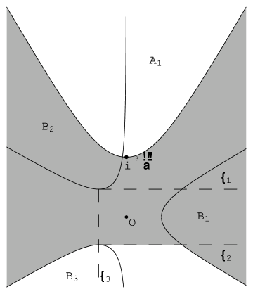
Figure 5. ${\rm Im}\,(u^{\prime}\bar{u})<0$ in the shaded area. Here $\ell_{1}:{\rm Im}\,z=\sqrt[3]{\beta/2},$ $\ell_{2}:{\rm Im}\,z=-\sqrt[3]{\beta/2}$ and $\ell_{3}:{\rm Re}\,z=-\sqrt[3]{\beta/2}$.

Mezincescu [18, §3] has previously observed that the eigenfunction has no zeros on the real axis, which obviously lies in the shaded region of Figure 5. Moreover, we see that all the zeros of $u$ and $u^{\prime}$ in ${\rm Im}\,z\geq 0$ must be in $A_{1}$.

Note that the lowest point in the closure $cl(B_{2})$ of $B_{2}$ is $-\sqrt[3]{\beta/2}+i\sqrt[3]{\beta/2}$.

Proof of Theorem  5.

For any $y\in\mathbb{R}$, by (4) with $z(t)=t+iy$ and by $u(\pm\infty+iy)=0=u^{\prime}(\pm\infty+iy)$, we have that

$${\rm Im}\,[u^{\prime}(x+iy)\bar{u}(x+iy)]=\int_{-\infty}^{x}{\rm Im}\,(iz(t)^{3}-\lambda)|u|^{2}dt,$$

and this is negative for $x+iy\in B_{4}$ with $|y|\leq\sqrt[3]{\beta/2}$, because then $z(t)=t+iy\in B_{4}$ for all $-\infty<t<x$ and so ${\rm Im}\,(iz(t)^{3}-\lambda)<0$.

This argument also shows that ${\rm Im}\,(u^{\prime}\bar{u})<0$ in $\{z\in B_{4}:{\rm Re}\,z\leq-\sqrt[3]{\beta/2}\}$; see Figure 5.

Similarly in $B_{1}$, for all $y$ we have that ${\rm Im}\,(u^{\prime}\bar{u})=-\int_{x}^{\infty}{\rm Im}\,(iz(t)^{3}-\lambda)|u(t+iy)|^{2}dt<0$.

For $z\not\in A_{1}\text{ with }{\rm Im}\,z\geq\sqrt[3]{\beta/2}$ (so that $z\in A_{4}$), we use (4) along vertical line segments starting from points on the line ${\rm Im}\,z=\sqrt[3]{\beta/2}$ to conclude ${\rm Im}\,(u^{\prime}\bar{u})<0$ in this region. ∎

Note that ${\rm Im}\,(u^{\prime}\bar{u})=-\frac{1}{2}\frac{\partial}{\partial y}|u(x+iy)|^{2}$. So in the region in Theorem 5, $|u(x+iy)|$ is an increasing function of $y.$

Theorem 6.

Assume $\beta>0$. Then

(i) ${\rm Re}\,(u^{\prime}\bar{u})>0$ on the union of the regions $A_{2}$, the region below $A_{2}$ and the region $\mathcal{R}\subset B_{4}$ between $A_{2}$ and $B_{2}$ with the real part less than or equal to that of the zero $\omega_{3}$ of $iz^{3}-\lambda$ in the third quadrant. See Figure 7.

(ii) ${\rm Re}\,(u^{\prime}\bar{u})<0$ on the union of the regions $A_{3}$, the region below $A_{3}$, and the region in $B_{1}$ with the real part greater than or equal to that of the zero $\omega_{4}$ of $iz^{3}-\lambda$ in the fourth quadrant. See Figure 7.

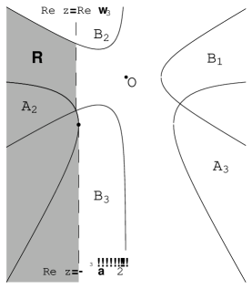
Figure 6. ${\rm Re}\,(u^{\prime}\bar{u})>0$ in the shaded area.

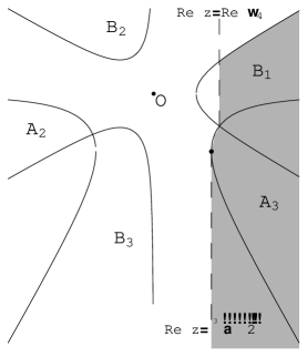
Figure 7. ${\rm Re}\,(u^{\prime}\bar{u})<0$ in the shaded area.

Obviously $iz^{3}-\lambda$ has three zeros. When $\beta>0$, one of the zeros is in the second quadrant, one $\omega_{3}$ in the third and one $\omega_{4}$ in the fourth quadrant. Certainly these are the three points at which the boundaries of the $A_{i}$ and $B_{i}$ intersect.

Theorem 2 with $n=1$ shows that $\frac{|\beta|}{\alpha}\leq\tan\frac{\pi}{5}\approx 0.73.$ It is easy to see that the rightmost point of $cl(A_{2})$ is $\sqrt[3]{\frac{\alpha}{2}}(-1-i)$, at which ${\rm Im}\,(iz^{3}-\lambda)=x^{3}-3xy^{2}-\beta>0$ by $0<\beta<\alpha$. Thus the rightmost point of $cl(A_{2})$ lies inside $B_{3}$ as shown in Figure 7. Similarly, the leftmost point of $cl(A_{3})$ is $\sqrt[3]{\frac{\alpha}{2}}(1-i)$, at which ${\rm Im}\,(iz^{3}-\lambda)=x^{3}-3xy^{2}-\beta<0$. Thus the leftmost point of $cl(A_{3})$ lies outside $B_{1}$ as shown in Figure 7.

Proof of Theorem  6.

In the regions $A_{2}$ and $A_{3}$, we use (4) with horizontal lines to infinity to get the statements in parts $(i)$ and $(ii)$ of this theorem. In the region $\mathcal{R}$ between $A_{2}$ and $B_{2}$ with the real part less than or equal to that of the zero of $iz^{3}-\lambda$ in the third quadrant (see Figure 7), we use (4) with vertical lines $z(t)=x+it$ to show that ${\rm Re}\,(u^{\prime}\bar{u})>0$. That is, we use $\left.{\rm Re}\,(u^{\prime}\bar{u})\right|_{x+ic}^{x+id}=-\int_{c}^{d}{\rm Im}\,(iz(t)^{3}-\lambda)|u(x+it)|^{2}dt$. If $x+id\in\mathcal{R}$, we can find $x+ic\in cl(A_{2}\cap B_{3}^{c})$, so that ${\rm Re}\,[u^{\prime}(x+ic)\bar{u}(x+ic)]>0$, and $-{\rm Im}\,(iz(t)^{3}-\lambda)>0$. Hence, the above integral is an increasing function of $d$. Hence we have the desired result in this region $\mathcal{R}$.

The region below $A_{2}$ is contained in $B_{3}$ since the rightmost point of $cl(A_{2})$ lies in $B_{3}$ (see Figure 7). So a similar argument shows that ${\rm Re}\,(u^{\prime}\bar{u})>0$ in the region below $A_{2}$. Also, the region below $A_{3}$ is contained in $B_{4}$ (see Figure 7) and so modified arguments show that the other statements of this theorem in part $(ii)$ are true. ∎

Corollary 7.

When ${\rm Im}\,\lambda=\beta>0$, the zero-free region of $u$ and $u^{\prime}$ contains the union of the three shaded regions in Figure 5, 7 and 7.

Note that in case ${\rm Im}\,\lambda=\beta<0$ we can get similar theorems corresponding to the above two, since $\bar{u}(-\bar{z})$ is an eigenfunction with eigenvalue $\bar{\lambda}$. The regions involved are simply the reflections of the above with respect to the imaginary axis.

In case $\beta=0$, so that $\lambda$ is real and $\lambda=\alpha>0$, the regions $B_{1},B_{2},B_{3}$ degenerate to the sectors $\{-\frac{\pi}{6}<\arg z<\frac{\pi}{6}\},\{\frac{\pi}{2}<\arg z<\frac{5\pi}{6}\},\{-\frac{5\pi}{6}<\arg z<-\frac{\pi}{2}\}$ respectively, and we get the following theorem on zero-free regions.

Theorem 8.

Suppose $\lambda$ is real. Then ${\rm Im}\,(u^{\prime}\bar{u})<0$ on $\{-\frac{\pi}{6}\leq\arg z\leq\frac{7\pi}{6}\}-A_{1}$ (which is a degenerate case of Figure 5), while ${\rm Re}\,(u^{\prime}\bar{u})$ behaves as in Figure 7 and 7 with $B_{1},B_{2},B_{3}$ being sectors as above.

Also ${\rm Re}\,(u^{\prime}\bar{u})<0$ in $cl(A_{1})\cap\{{\rm Re}\,z<0\}$ and ${\rm Re}\,(u^{\prime}\bar{u})>0$ in $cl(A_{1})\cap\{{\rm Re}\,z>0\}$.

Corollary 9.

When $\lambda$ is real, the zero-free region of $u$ and $u^{\prime}$ contains the union of all regions in Theorem 8; see Figure 8. That is, $u$ and $u^{\prime}$ can only have zeros in $\{iy:y>\sqrt[3]{\lambda}\}$

$$\cup\left\{z\in A_{4}:-\frac{5\pi}{6}<\arg z<-\frac{\pi}{6},{\rm Im}\,z>-\sqrt[3]{\lambda/2}\right\}\cup\left\{z:|{\rm Re}\,z|<\sqrt[3]{\lambda/2},{\rm Im}\,z\leq-\sqrt[3]{\lambda/2}\right\}.$$

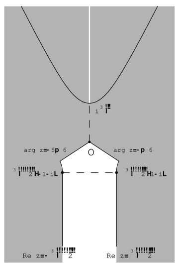
Figure 8. When $\lambda$ is real, the shaded area is the zero-free region of $u$ and $u^{\prime}$.

Remark 8.

Bender et al. [4] find numerically that $u$ has some zeros along an “arch” within the unshaded region in Figure 8, when $\lambda$ is real.

In proving Theorem 8, we will use the following lemma.

Lemma 10.

Suppose $\zeta\in A_{1}$, ${\rm Re}\,(u^{\prime}\bar{u})=0$ at $\zeta$. Then ${\rm Re}\,(u^{\prime}\bar{u})<0$ at all $\zeta-t\in A_{1},t>0$ and ${\rm Re}\,(u^{\prime}\bar{u})>0$ at all $\zeta+t\in A_{1},t>0$.

Note that there is no restriction on the sign of ${\rm Im}\,\lambda$, in this lemma.

Proof.

On horizontal line segments $z(t)=t+iy$ in $A_{1}$, (4) becomes

$$\left.{\rm Re}\,(u^{\prime}\bar{u})\right|_{c+iy}^{d+iy}=\int_{c}^{d}|u_{x}(z(t))|^{2}dt+\int_{c}^{d}{\rm Re}\,(iz^{3}(t)-\lambda)|u(z(t))|^{2}dt.$$

Since ${\rm Re}\,(iz^{3}(t)-\lambda)>0$ in $A_{1}$, ${\rm Re}\,(u^{\prime}\bar{u})$ is a strictly increasing function of $x$ on each horizontal line segment in $A_{1}$. ∎

Proof of Theorem  8.

The proofs of Theorems 5 and 6 give everything except the last statement of the theorem. For that, recall we can take $u(z)=\bar{u}(-\bar{z})$ by Remark 3; this implies ${\rm Re}\,(u^{\prime}\bar{u})$ is an odd function with respect to reflection in the imaginary axis, so ${\rm Re}\,(u^{\prime}\bar{u})=0$ on the whole imaginary axis. Now we use Lemma 10 to complete the proof. ∎

By the last statement of Lemma 1, in the sector $S_{-1,\frac{\pi}{20}}$ that contains the negative imaginary axis, the eigenfunction $u$ has only finitely many zeros. Now with the zero-free region in the Theorems 6 and 8, we see that $u$ has only finitely many zeros in ${\rm Im}\,z<0$. Since $u$ has infinitely many zeros, $u$ must have infinitely many zeros in ${\rm Im}\,z\geq 0$. When $\beta>0$ (hence when $\beta<0$ as well), by Theorem 5, $u$ must have infinitely many zeros in $A_{1}$. Also when $\beta=0$, by Theorem 8, $u$ has infinitely many zeros on the positive imaginary axis.

The next theorem gives some information on how zeros of $u$ and $u^{\prime}$ in $A_{1}$ should be arranged, when $\beta>0$. Note that all the zeros of $u$ and $u^{\prime}$ in ${\rm Im}\,z\geq 0$ lie in $A_{1}$ by Theorem 5.

Theorem 11.

Suppose $u(z)$ is an eigenfunction of (13) with eigenvalue $\lambda\in\mathbb{C}$ with ${\rm Im}\,\lambda=\beta>0$. Then

(i) ${\rm Re}\,(u^{\prime}\bar{u})\geq 0$ for some point on the imaginary axis if and only if $uu^{\prime}$ has infinitely many zeros in $A_{1}\cap B_{2}$ and at most finitely many zeros in $A_{1}\cap B_{2}^{c}$; and

(ii) ${\rm Re}\,(u^{\prime}\bar{u})<0$ for every point on the imaginary axis if and only if $uu^{\prime}$ has no zeros in $\{z\in A_{1}:{\rm Re}\,z\leq 0\}$ and infinitely many in $\{z\in A_{1}:{\rm Re}\,z>0\}$.

We will use the following lemma along with Lemma 10.

Lemma 12.

Assume ${\rm Im}\,\lambda=\beta>0$. Suppose ${\rm Re}\,\zeta_{1}\leq{\rm Re}\,\zeta_{2}$ and ${\rm Re}\,(u^{\prime}\bar{u})=0$ at $\zeta_{1}$, $\zeta_{2}$ $(\text{where }\zeta_{1}\not=\zeta_{2})$. Then

(i) $\zeta_{1},\zeta_{2}\in cl(A_{1}\cap B_{2})\Longrightarrow$ ${\rm Re}\,\zeta_{1}<{\rm Re}\,\zeta_{2}$ and ${\rm Im}\,\zeta_{1}<{\rm Im}\,\zeta_{2}$, and

(ii) $\zeta_{1},\zeta_{2}\in cl(A_{1}\cap B_{2}^{c})\Longrightarrow$ ${\rm Re}\,\zeta_{1}<{\rm Re}\,\zeta_{2}$ and ${\rm Im}\,\zeta_{1}>{\rm Im}\,\zeta_{2}$.

Proof of part (i).

We will first prove this for $\zeta_{1},\zeta_{2}\in A_{1}\cap B_{2}$. Suppose that ${\rm Re}\,\zeta_{1}={\rm Re}\,\zeta_{2}$. Then we could find a vertical line segment $z(t)$ in $A_{1}\cap B_{2}$ whose end points are $\zeta_{1}$ and $\zeta_{2}$. We apply (4) to this line segment to get

$$0=-\int_{c}^{d}{\rm Im}\,(iz^{3}(t)-\lambda)|u(z(t))|^{2}dt.$$

This would imply $u\equiv 0$ on the curve $z(t)$ since ${\rm Im}\,(iz^{3}(t)-\lambda)>0$ in $B_{2}$. So then since $u$ is analytic, $u\equiv 0$ in $\mathbb{C}$. This is a contradiction. Hence ${\rm Re}\,\zeta_{1}<{\rm Re}\,\zeta_{2}$.

Similarly, suppose that ${\rm Im}\,\zeta_{1}\geq{\rm Im}\,\zeta_{2}$. Then we could find a smooth curve $z(t)=x(t)+iy(t)$ in $A_{1}\cap B_{2}$ such that $z(c)=\zeta_{1}$, $z(d)=\zeta_{2}$, $x^{\prime}(t)>0$ and $y^{\prime}(t)\leq 0$. Note that ${\rm Im}\,(iz^{3}(t)-\lambda)>0$ and ${\rm Re}\,(iz^{3}(t)-\lambda)>0$ in $A_{1}\cap B_{2}$. This contradicts (4) like for the case of ${\rm Re}\,\zeta_{1}={\rm Re}\,\zeta_{2}$. We now see that the above argument still holds for $\zeta_{1},\zeta_{2}\in cl(A_{1}\cap B_{2})$.

Proof of part (ii). We use (4) again and a similar argument like in the proof of part $(i)$. ∎

Figure 9.

Proof of Theorem  11.

Suppose $u(z)$ is an eigenfunction of (13) with eigenvalue $\lambda\in\mathbb{C}$ with ${\rm Im}\,\lambda=\beta>0$. Since $u$ has infinitely many zeros in $A_{1}$ (by the paragraph shortly before Theorem 11), certainly $uu^{\prime}$ also has infinitely many zeros in $A_{1}$.

Proof of part (i). Suppose that ${\rm Re}\,(u^{\prime}\bar{u})\geq 0$ for some point $iy$ on the imaginary axis. By (4) with $z(t)=it$, we have that

(16) $$\left.{\rm Re}\,(u^{\prime}\bar{u})\right|_{ic}^{id}=\beta\int_{c}^{d}|u(iy)|^{2}dy.$$

So then since $\beta>0$, ${\rm Re}\,(u^{\prime}\bar{u})>0$ at every point $it$ for $t>y$. Now by Lemma 10, we have that ${\rm Re}\,(u^{\prime}\bar{u})>0$ at every $x+it\in A_{1}$ for $t>y$ and $x\geq 0$. Thus $uu^{\prime}$ does not have any zeros in $\{z\in A_{1}\cap B_{2}^{c}:{\rm Re}\,z\geq 0,{\rm Im}\,z>y\}$.

The entire function $uu^{\prime}$ does not have infinitely many zeros in any bounded region. So if $uu^{\prime}$ had infinitely many zeros in $A_{1}\cap B_{2}^{c}$, then $uu^{\prime}$ would have infinitely many zeros in $\{z\in A_{1}\cap B_{2}^{c}:{\rm Re}\,z<0\}$. But if $uu^{\prime}$ has a zero $z_{1}$ in $\{z\in A_{1}\cap B_{2}^{c}:{\rm Re}\,z<0\}$, then by Lemma 12 $(ii)$, $uu^{\prime}$ has no zeros in $\{z\in A_{1}\cap B_{2}^{c}:{\rm Re}\,z_{1}\leq{\rm Re}\,z<0\}$. So then $uu^{\prime}$ would have infinitely many zeros in a bounded region. This is a contradiction. Thus $uu^{\prime}$ has infinitely many zeros in $A_{1}\cap B_{2}$ and at most finitely many zeros in $A_{1}\cap B_{2}^{c}$.

Conversely, suppose that $uu^{\prime}$ has infinitely many zeros in $A_{1}\cap B_{2}$ and at most finitely many zeros in $A_{1}\cap B_{2}^{c}$. Choose a zero $z_{0}$ in $A_{1}\cap B_{2}$. Then by Lemma 10, we see that ${\rm Re}\,(u^{\prime}\bar{u})>0$ at $i{\rm Im}\,z_{0}$ since ${\rm Re}\,z_{0}<0$.

Proof of part (ii). Suppose that ${\rm Re}\,(u^{\prime}\bar{u})<0$ for every point on the imaginary axis. Then by Lemma 10, ${\rm Re}\,(u^{\prime}\bar{u})<0$ for every point in $\{z\in A_{1}:{\rm Re}\,z\leq 0\}$. So then $uu^{\prime}$ has no zeros in $\{z\in A_{1}:{\rm Re}\,z\leq 0\}$. Now since we know that $uu^{\prime}$ has infinitely many zeros in $A_{1}$, $uu^{\prime}$ must have infinitely many zeros in $\{z\in A_{1}:{\rm Re}\,z>0\}$.

Conversely, suppose ${\rm Re}\,(u^{\prime}\bar{u})\geq 0$ for some point on the imaginary axis. Then $uu^{\prime}$ would have at most finitely many zeros in $\{z\in A_{1}:{\rm Re}\,z>0\}$ by the argument as in the proof of part $(i)$. This completes the proof. ∎

Remark 9.

Since the negative imaginary axis is in the middle of a blowing-up Stokes region (see Figure 2), $u(iy)$ blows up as $y$ tends to $-\infty$. On the other hand, the positive imaginary axis is a critical ray. We can show that $|u(iy)|^{2}\leq(const.)y^{-{\frac{3}{2}}}$ for all $y$ near positive infinity, by Theorem 7.4.4 in [16].

So the right-hand side of (16) approaches $+\infty$ as $c$ tends to $-\infty$ (while $d$ is fixed). Thus we see that ${\rm Re}\,[u^{\prime}(ic)\bar{u}(ic)]<0$ for all $c$ near negative infinity. However, the right-hand side of (16) is convergent as $d$ tends to $+\infty$ (while $c$ is fixed). So ${\rm Re}\,(u^{\prime}\bar{u})$ may or may not become positive near infinity along the positive imaginary axis.

The next lemma gives some information on zeros of $u$ and $u^{\prime}$ in ${\rm Im}\,z<0$, if any exist. There can only be finitely many such zeros, by the paragraph shortly before Theorem 11.

Lemma 13.

Assume ${\rm Im}\,\lambda=\beta\geq 0$. Suppose ${\rm Im}\,\zeta_{1}\leq{\rm Im}\,\zeta_{2}$ and ${\rm Im}\,(u^{\prime}\bar{u})=0$ at $\zeta_{1}$, $\zeta_{2}$ $(\text{where }\zeta_{1}\not=\zeta_{2})$. Then

(i) $\zeta_{1},\zeta_{2}\in cl(A_{4}\cap B_{3})\Longrightarrow$ ${\rm Im}\,\zeta_{1}<{\rm Im}\,\zeta_{2}$ and ${\rm Re}\,\zeta_{1}<{\rm Re}\,\zeta_{2}$, and

(ii) $\zeta_{1},\zeta_{2}\in cl(A_{4}\cap B_{4})\Longrightarrow$ ${\rm Im}\,\zeta_{1}<{\rm Im}\,\zeta_{2}$ and ${\rm Re}\,\zeta_{1}>{\rm Re}\,\zeta_{2}$.

Proof.

We omit the proof because it is very similar to the proof of Lemma 12. We use (4) instead of (4), and also make use of Figures 7 and 7. ∎

Roughly speaking, then, the zeros move up and to the right in the third quadrant, and down and to the right in the fourth quadrant. This observation supports that when $\lambda$ is real, zeros of $u$ in ${\rm Im}\,z<0$ lie on an arch-shaped curve as in Figures 5 and 6 in [4].

4. Other properties of eigenfunctions

Here we present a possible way of proving the conjecture that the eigenvalues $\lambda$ of $H=-\frac{d^{2}}{dz^{2}}-(iz)^{3}$ are positive real. Given an eigenfunction $u$ with eigenvalue $\lambda$, Theorem 14 below gives a class $\mathcal{O}$ of polynomials $p(x,y)$ which are orthogonal to $|u|^{2}$ in the sense that $\int_{-\infty}^{\infty}p(x,y)|u(x+iy)|^{2}dx=0$ for all $y$. One can perhaps prove the conjecture as follows. Suppose ${\rm Im}\,\lambda\not=0$; if $\mathcal{O}$ is large enough then $|u|^{2}\equiv 0$, giving a contradiction.

Let $u$ be an eigenfunction of $H=-\frac{d^{2}}{dz^{2}}-(iz)^{3}$ with eigenvalue $\lambda=\alpha+i\beta$.

Theorem 14.

Let $\mathcal{O}=\{\text{polynomials }p(\cdot,\cdot):\int_{-\infty}^{\infty}p(x,y)|u(x+iy)|^{2}dx=0\text{ for all $y$}\}$. Then:

(i) $x^{3}-3xy^{2}-\beta\in\mathcal{O}$,

(ii) for all $m\geq 0$,

$$\frac{4}{m+1}(\frac{x^{m+5}}{m+5}-3y^{2}\frac{x^{m+3}}{m+3}-\beta\frac{x^{m+2}}{m+2})(x^{3}-3y^{2}x-\beta)$$

$$-m(m-1)x^{m-2}-4x^{m}(3x^{2}y-y^{3}+\alpha)-\frac{12}{m+1}yx^{m+2} \in \mathcal{O},$$

(iii) if $p\in\mathcal{O}$ then $p_{y}+2(x^{3}-3xy^{2}-\beta)\int_{0}^{x}p(t,y)dt\in\mathcal{O}$, and

(iv) if $p\in\mathcal{O}$ then $p_{xx}+p_{yy}+12x^{2}yp+4(x^{3}-3xy^{2}-\beta)\int_{0}^{x}p_{y}(t,y)dt\in\mathcal{O}$.

For example the following polynomials are in $\mathcal{O}$:

$$p_{3}(x,y) = x^{3}-3xy^{2}-\beta,\text{ by $(i)$},$$

$$p_{7}(x,y) = x^{7}-9x^{5}y^{2}-5x^{4}\beta+18x^{3}y^{4}+18x^{2}y^{2}\beta+4x(\beta^{2}-3y),$$

$$\text{by applying $(iii)$ to $p_{3}$ and multiplying by 2},$$

$$p_{8}(x,y) = 2x^{8}-16x^{6}y^{2}-7x^{5}\beta+30x^{4}y^{4}+25x^{3}y^{2}\beta+5x^{2}(\beta^{2}-12y)+10y^{3}-10\alpha,$$

by applying $$(ii) m=0 \frac{5}{2}$$ with and multiplying by ,

$$p_{9}(x,y) = 2x^{9}-15x^{7}y^{2}-6x^{6}\beta+27x^{5}y^{4}+4x^{3}(\beta^{2}-27y)+24xy^{3}+21x^{4}y^{2}\beta-24x\alpha,$$

by applying $$(ii) m=1 6$$ with and multiplying by , and

$$p_{10}(x,y) = 20x^{10}-144x^{8}y^{2}-55x^{7}\beta+252x^{6}y^{4}+189x^{5}y^{2}\beta-35x^{4}(48y-\beta^{2})$$

$$+420x^{2}(y^{3}-\alpha)-210,\text{ by applying $(ii)$ with $m=2$ and multiplying by $105$.}$$

We do not know whether Theorem 14 generates all the polynomials in $\mathcal{O}$.

Proof of Theorem  14.

It is useful to have the following two formulas, which follow from multiplying (13) by $\bar{u}$ and separating real and imaginary parts:

(17) $${\rm Im}\,[u_{x}(x+iy)\bar{u}(x+iy)]_{x}=(x^{3}-3xy^{2}-\beta)|u(x+iy)|^{2}$$

and

(18) $${\rm Re}\,[u_{x}(x+iy)\bar{u}(x+iy)]_{x}=|u_{x}|^{2}+(-3x^{2}y+y^{3}-\alpha)|u|^{2}.$$

At the end of the proof we will justify the fact that we can differentiate through the integrals that follow.

$(i)$ This is clear by integrating (17), using the zero boundary conditions in the left- and right-hand Stokes regions.

$(ii)$ Suppose $m$ is a nonnegative integer. Then

$$\frac{d}{dy}\int_{-\infty}^{\infty}x^{m}|u|^{2}dx=\int_{-\infty}^{\infty}x^{m}\frac{\partial}{\partial y}|u|^{2}dx = -2\int_{-\infty}^{\infty}x^{m}{\rm Im}\,(u_{x}\bar{u})dx$$

$$= \frac{2}{m+1}\int_{-\infty}^{\infty}x^{m+1}{\rm Im}\,(u_{x}\bar{u})_{x}dx,$$

where the last step is by integration by parts.

So using (17), we have that

$$\frac{d}{dy}\int_{-\infty}^{\infty}x^{m}|u|^{2}dx=\frac{2}{m+1}\int_{-\infty}^{\infty}x^{m+1}(x^{3}-3xy^{2}-\beta)|u|^{2}dx.$$

Hence,

$$\frac{d^{2}}{dy^{2}}\int_{-\infty}^{\infty}x^{m}|u(x+iy)|^{2}dx$$

$$= \frac{2}{m+1}\int_{-\infty}^{\infty}[-6x^{m+2}y|u|^{2}-2(x^{m+4}-3x^{m+2}y^{2}-\beta x^{m+1}){\rm Im}\,(u_{x}\bar{u})]dx.$$

Then again using the integration by parts and (17), we have that this equals

(20) $$\frac{2}{m+1}\int_{-\infty}^{\infty}[-6x^{m+2}y+2(\frac{x^{m+5}}{m+5}-3y^{2}\frac{x^{m+3}}{m+3}-\beta\frac{x^{m+2}}{m+2})(x^{3}-3xy^{2}-\beta)]|u|^{2}dx.$$

Also, we differentiate (4) without applying integration by parts:

(21) $$\frac{d^{2}}{dy^{2}}\int_{-\infty}^{\infty}x^{m}|u|^{2}dx = -2\int_{-\infty}^{\infty}x^{m}[{\rm Re}\,(u_{x}\bar{u})_{x}-2|u_{x}|^{2}]dx$$

(22) $$= -2\int_{-\infty}^{\infty}x^{m}[(-3x^{2}y+y^{3}-\alpha)|u|^{2}-|u_{x}|^{2}]dx\quad\text{by (\ref{real-diff})}.$$

Also, applying integration by parts twice to the right-hand side of (21), we have that (21) equals

(23) $$-m(m-1)\int_{-\infty}^{\infty}x^{m-2}|u|^{2}dx+4\int_{-\infty}^{\infty}x^{m}|u_{x}|^{2}dx.$$

By equating (22) and (23), we get

(24) $$\int_{-\infty}^{\infty}x^{m}|u_{x}|^{2}dx=\frac{m(m-1)}{2}\int_{-\infty}^{\infty}x^{m-2}|u|^{2}dx-\int_{-\infty}^{\infty}x^{m}(-3x^{2}y+y^{3}-\alpha)|u|^{2}dx.$$

Hence equating (20) and (22) and substituting (24) give $(ii)$.

$(iii)$ Suppose that $\int_{-\infty}^{\infty}p(x,y)|u|^{2}dx=0\text{ for all $y$}$. Then

$$0 = \frac{d}{dy}\int_{-\infty}^{\infty}p(x,y)|u|^{2}dx$$

$$= \int_{-\infty}^{\infty}[p_{y}(x,y)|u|^{2}-2p(x,y){\rm Im}\,(u_{x}\bar{u})]dx$$

$$= \int_{-\infty}^{\infty}\left[p_{y}(x,y)|u|^{2}+2\biggl{\{}\int_{0}^{x}p(t,y)dt\biggr{\}}{\rm Im}\,(u_{x}\bar{u})_{x}\right]dx,$$

by integration by parts. This with (17) gives $(iii)$.

$(iv)$ Suppose $\int_{-\infty}^{\infty}p(x,y)|u|^{2}dx=0\text{ for all }y$.

Then we differentiate through (4) with respect to $y$ again to get

$$0 = \int_{-\infty}^{\infty}\left[p_{yy}(x,y)|u|^{2}-4p_{y}(x,y){\rm Im}\,(u_{x}\bar{u})-2p(x,y){\rm Im}\,(iu_{xx}\bar{u}-i|u_{x}|^{2})\right]dx$$

$$= \int_{-\infty}^{\infty}\left[p_{yy}(x,y)|u|^{2}+4\biggl{\{}\int_{0}^{x}p_{y}(t,y)dt\biggr{\}}{\rm Im}\,(u_{x}\bar{u})_{x}-2p(x,y)({\rm Re}\,(u_{x}\bar{u})_{x}-2|u_{x}|^{2})\right]dx$$

$$= \int_{-\infty}^{\infty}\left[p_{yy}(x,y)+4\biggl{\{}\int_{0}^{x}p_{y}(t,y)dt\biggr{\}}(x^{3}-3xy^{2}-\beta)\right]|u|^{2}dx$$

$$-2\int_{-\infty}^{\infty}p(x,y)\left[-{\rm Re}\,(u_{x}\bar{u})_{x}+2(-3x^{2}y+y^{3}-\alpha)|u|^{2}\right]dx,\qquad\text{by (\ref{im-diff}) and (\ref{real-diff})}$$

$$= \int_{-\infty}^{\infty}\left[p_{yy}(x,y)+4\biggl{\{}\int_{0}^{x}p_{y}(t,y)dt\biggr{\}}(x^{3}-3xy^{2}-\beta)-4p(x,y)(-3x^{2}y+y^{3}-\alpha)\right]|u|^{2}dx$$

$$-\int_{-\infty}^{\infty}p_{x}(x,y)2{\rm Re}\,(u_{x}\bar{u})dx.$$

But $(y^{3}-\alpha)\int_{-\infty}^{\infty}p|u|^{2}dx=0$, and so applying integration by parts again to the last term gives $(iv)$.

Now to complete the proof we need to show that we can differentiate through the above integrals, which reduces to showing that

$$\frac{d}{dy}\int_{-\infty}^{\infty}x^{m}|u|^{2}dx=\int_{-\infty}^{\infty}x^{m}\frac{\partial}{\partial y}|u|^{2}dx,\qquad\text{for each $m\geq 0$}.$$

So we estimate the following:

$$\biggl{|}\int_{-\infty}^{\infty}x^{m}[\frac{1}{h}\{|u(x+i(y+h))|^{2}-|u(x+iy)|^{2}\}-\frac{\partial}{\partial y}|u(x+iy)|^{2}]dx\biggr{|}$$

$$\leq \int_{-\infty}^{\infty}|x|^{m}\bigl{|}\frac{1}{h}\{|u(x+i(y+h))|^{2}-|u(x+iy)|^{2}\}-\frac{\partial}{\partial y}|u(x+iy)|^{2}\bigr{|}dx$$

$$\leq |h|\int_{-\infty}^{\infty}|x|^{m}\bigl{|}\frac{\partial^{2}(|u|^{2})}{\partial y^{2}}(x+i\xi(x))\bigr{|}dx,\quad\text{by the Mean Value Theorem,}$$

where $|\xi(x)-y|\leq|h|.$

So then it is enough to show that for each $M>0$, there exist $C_{1}>0$ and $C_{2}>0$ such that

(26) $$|u(x+iy)|+|u^{\prime}(x+iy)|+|u^{\prime\prime}(x+iy)|\leq\frac{C_{1}}{\exp[|x|^{C_{2}}]}\qquad\text{for all}\quad|y|\leq M.$$

Proof of (26) is as follows:

Suppose that $z=re^{i\theta}$ with $|\theta|\leq\frac{\pi}{20}$. Then $z$ is in the decaying Stokes regions (see Figure 2). By the asymptotic expression (5) we get that for some $C>0$, $|u(re^{i\theta})|\leq\exp[-|r|^{C}]$ for all $|\theta|\leq\frac{\pi}{20}$ and large $|r|$, say $|r|\geq R$. Also choose $R\geq M+1$.

Now the Cauchy integral formula says that

$$u^{(k)}(z)=\frac{k!}{2\pi i}\int_{|\zeta-z|=1}\frac{u(\zeta)}{(\zeta-z)^{k+1}}d\zeta.$$

So then

$$|u^{(k)}(z)|\leq\frac{k!}{2\pi}\int_{|\zeta-z|=1}|u(\zeta)||d\zeta|\leq k!\max\{|u(\zeta)|:|\zeta-z|=1\}\leq k!\exp[-(|z|-1)^{C}]$$

where the last inequality holds if $\{\zeta\in\mathbb{C}:|\zeta-z|=1\}\subset\{\zeta\in\mathbb{C}:\zeta=\rho e^{i\phi},|\rho|\geq R,|\phi|\leq\frac{\pi}{20}\}$.

Choose $0<C_{2}<C$. Then $\exp[-(|z|-1)^{C}]\leq\exp[-|z|^{C_{2}}]$ if $|z|\geq R_{2}$ for large $R_{2}\geq R$.

The region where $|z|\geq R_{2}$ and $\{\zeta\in\mathbb{C}:|\zeta-z|=1\}\subset\{\zeta\in\mathbb{C}:\zeta=\rho e^{i\phi},|\rho|\geq R,|\phi|\leq\frac{\pi}{20}\}$ covers all of $|y|\leq M$ but a bounded region.

Since the minimum of $\exp[-|z|^{C_{2}}]$ in this bounded region is strictly positive, we can find a large $C_{1}>0$ so that the left-hand side of (26) is bounded by $C_{1}\exp[-|z|^{C_{2}}]$. Thus (26) holds since $|x|\leq|z|$. And this completes the proof. ∎

Corollary 15.

Let $u(z)$ be an eigenfunction of (13). Then $\int_{-\infty}^{\infty}|u(x+iy)|^{2}dx$ is a convex function.

Proof.

This is a consequence of (23) with $m=0$, or it can be proved using the subharmonicity of $|u|^{2}.$ ∎

5. Conclusions

Using simple path integrations, we were able to prove that eigenvalues of (1) lie in the sector $|\arg\lambda|\leq\frac{\pi}{2n+3}$ and we extended the result for some more general Hamiltonians. Also we provide zero-free regions of eigenfunctions and their first derivatives, for the potential $-(ix)^{3}$. Then finally we have the set $\mathcal{O}$ of polynomials $p(x,y)$ which are orthogonal to $|u|^{2}$ in the sense that $\int_{-\infty}^{\infty}p(x,y)|u|^{2}dx=0$ for all $y$.

In a recent communication with Mezincescu, he pointed out that for the potential $-(ix)^{3}$ if ${\rm Im}\,\lambda=\beta\not=0$, combining $\frac{|\beta|}{\alpha}\leq\tan\frac{\pi}{5}$ with the equation ($23$) in [18] gives $|\lambda|>(\frac{2}{5}\cos\frac{\pi}{5})10^{5}\approx 3\times 10^{4}.$ So if any non-real eigenvalues exist, they are very large.

In this paper we consider only polynomial potentials with odd degrees. However, a number of other authors have worked on even degree potentials, particularly quartic [11, 19] and sextic [1, 6] polynomial potentials. Our techniques in proving Theorems 2 and 3 can be used to get information on eigenvalues for even degree potentials if both ends of a line passing through the origin stay in decaying Stokes regions.

Obvious open problems are to narrow the eigenvalue sectors closer to the positive real axis, and finally to prove that the eigenvalues are real. Since some $\mathcal{PT}$-symmetric non-Hermitian Hamiltonians do not have all real eigenvalues, one might further want to classify $\mathcal{PT}$-symmetric non-Hermitian Hamiltonians which do have positive real eigenvalues.

Acknowledgments

The author was partially supported by NSF grant number DMS-9970228. The author appreciates Gary Gundersen’s help at the initial stage and Carl Bender’s comments later on, and thanks Richard S. Laugesen for encouragement, invaluable suggestions and discussions throughout the work.

email contact: kcshin@math.uiuc.edu

References

[1]
C. M. Bender.
Analytic continuation of eigenvalue problems.
Physics Letter A, 173:442–446, 1993.
[2]
C. M. Bender and S. Boettcher.
Real spectra in non-Hermitian Hamiltonians having symmetry.
Physical Review Letters, 80(24):5243–5246, 1998.
[3]
C. M. Bender, S. Boettcher and P. N. Meisinger.
-symmetric quantum mechanics.
Journal of Mathematical Physics, 40(5):2201–2229,
1999.
[4]
C. M. Bender, S. Boettcher and V. M. Savage.
Conjecture on the interlacing of zeros in complex Sturm-Liouville problems.
Preprint arXiv:math-ph/0005012;http://front.math.ucdavis.edu, 2000.
[5]
C. M. Bender, F. Cooper, P. N. Meisinger and V. M. Savage.
Variational ansatz for -symmetric quantum mechanics.
Physics Letter A, 259:224–231, 1999.
[6]
B. Bagchi, F. Cannata and C. Quesne.
-symmetric sextic potentials.
Physics Letter A, 269:79–82, 2000.
[7]
C. M. Bender and G. V. Dunne.
Large-order perturbation theory for a non-Hermitian
-symmetric Hamiltonian.
Journal of Mathematical Physics, 40(10):4616–4621,
1999.
[8]
M. P. Blencowe, H. F. Jones and A. P. Korte.
Applying the linear expansion to the
interaction.
Physical Review D, 57(8):5092–5099, 1998.
[9]
E. Caliceti.
Distributional Borel summability of odd anharmonic oscillators.
Journal of Physics A: Mathematical and General, 33(20):3753–3770, 2000.
[10]
E. Caliceti, S. Graffi and M. Maioli.
Perturbation theory of odd anharmonic oscillators.
Communications in Mathematical Physics, 75(51):51–66,
1980.
[11]
A. S. de Castro and A. de Souza Dutra.
Approximate analytical states of a polynomial potential: an example of symmetry restoration.
Physics Letters A, 269:281–286, 2000.
[12]
E. Delabaere and F. Pham.
Eigenvalues of complex Hamiltonians with -symmetry. I, II.
Physics Letters A, 250:25–32, 1998.
[13]
G. G. Gundersen.
On the real zeros of solutions of where
is entire.
Annales Academiæ Scientiarum Fennicæ Series
A. I. Mathematica., 11:275–294, 1986.
[14]
N. Hatano and D. R. Nelson.
Localization transitions in non-Hermitian quantum mechanics.
Physical Review Letters, 77(3):570–573, 1996.
[15]
N. Hatano and D. R. Nelson.
Vortex pinning and non-Hermitian quantum mechanics.
Physical Review B, 56(14):8651–8673, 1997.
[16]
E. Hille.
Lectures on ordinary differential equations.
Addison-Wesley, Reading. Massachusetts, 1969.
[17]
T. Kato.
Perturbation theory for linear operators.
Springer-Verlag, Berlin, 1966.
[18]
G. A. Mezincescu.
Some properties of eigenvalues and eigenfunctions of the
cubic oscillator with imaginary coupling constant.
Journal of Physics A: Mathematical and General, July, 2000.
[19]
O. Mustafa and M. Odeh.
Anharmonic oscillator energies via artificial perturbation method.
The European Physical Journal B, 15:143–148, 2000.
[20]
D. R. Nelson and N. M. Shnerb.
Non-Hermitian localization and population biology.
Physical Review E, 58(2):1383–1403, 1998.