Limitations on the smooth confinement of an unstretchable manifold

Abstract

We prove that an $m$-dimensional unit ball $D^{m}$ in the Euclidean space ${\mathbb{R}}^{m}$ cannot be isometrically embedded into a higher-dimensional Euclidean ball $B_{r}^{d}\subset{\mathbb{R}}^{d}$ of radius $r<1/2$ unless one of two conditions is met –

1. The embedding manifold has dimension $d\geq 2m$.

2. The embedding is not smooth.

The proof uses differential geometry to show that if $d<2m$ and the embedding is smooth and isometric, we can construct a line from the center of $D^{m}$ to the boundary that is geodesic in both $D^{m}$ and in the embedding manifold ${\mathbb{R}}^{d}$. Since such a line has length 1, the diameter of the embedding ball must exceed 1.

I Introduction

Mechanical deformation of objects is a part of our everyday experience. Objects like coil springs, wrapping films or blood cells are designed to be deformed in specified ways. Clearly the shape of an object influences how it may be deformed. We will be interested in looking at how the intrinsic geometry of an object restricts the ways in which the object can be deformed.

The mathematical notion of a Riemannian manifold gives a way of describing the shape of an object and its deformation. A Riemannian manifold is a set that has the topological structure of an Euclidean space ${\mathbb{R}}^{n}$ locally and is equipped with a local measure of distance, called the metric. An interesting question about two-dimensional or one-dimensional objects (manifolds) in three dimensional space is whether they can be deformed “isometrically”— that is, without changing lengths of lines in the object. Since an isometric deformation of a material causes no stretching, it is of practical importance to know what kinds of deformation can be made isometrically.

A classical problem in differential geometry is the study of isometric embeddings of a flat 2-dimensional sheet in ${\mathbb{R}}^{3}$. This is the study of developable surfaces DiffGeom1 ; DiffGeom2 . This problem has seen a recent resurgence of interest Pomeau ; cones_exp ; cones_thry ; maha ; Basile because of its connections with the nature of the singularities in a crumpled sheet buckling ; buckling2 ; acoustic ; cornell ; Li-Witten ; wit.sci .

Differential geometers are interested in the much more general question of whether a given manifold can be embedded in another manifold isometrically. A sphere and a Möbius strip are examples of $2$ dimensional manifolds that cannot be isometrically embedded in ${\mathbb{R}}^{2}$ but can be isometrically embedded in ${\mathbb{R}}^{3}$. There is a fundamental theorem, due to Nash nash showing that every manifold can be embedded in an Euclidean Space ${\mathbb{R}}^{d}$ of a sufficiently large dimension. However, the smallest dimension which allows this embedding depends on the additional structure imposed on the manifold and the embedding, and is the subject of current research. A more complete discussion of this question and improvements of Nash’s results can be found in references GR ; Gro .

In this paper we study the confinability of an embedded manifold. We will say that a $m$ dimensional object is confinable in $d$ dimensions if it is possible to smoothly deform the object without inducing any stretching so that it lies inside an arbitrarily small $d$ dimensional sphere. Of course, for this to make sense, we need $d>m$. Note that $d>m$ does not imply that such deformations are always possible. A two dimensional sheet confined in a shrinking sphere develops singularities – a phenomenon described informally as crumpling. Thus there is a lower bound on the size of the enclosing sphere which can contain the sheet smoothly and isometrically, that is without any stretching. We show below that this bound exists whenever the embedding space has fewer than twice the dimensions of the embedded manifold: the greatest distance between two embedded points, or the “span” of the embedded sheet, must be at least half the intrinsic diameter of the sheet. The converse of our theorem states that an $m$-dimensional manifold may be confined into an arbitrarily small sphere in ${\mathbb{R}}^{2m}$. This converse may be readily shown by an explicit construction Kramer.PRL .

The paper is organized as follows – We begin by discussing the problem in Section. II. In this section, we also illustrate the ideas behind our proof using the case of a two-sheet embedded in 3 dimensions. Section III.1 reviews the theorems of differential geometry on which our theorem is based, and Section III.2 contains the proof of the theorem, together with the proofs of seven lemmas used in the proof of the theorem. Section IV discusses implications of the theorem, related ideas, and possible generalizations.

In the body of the paper, we use many standard definitions and results from differential geometry. For completeness, we include an appendix, where we discuss some of these definitions and results. In this appendix, we have appended brief remarks to the standard definitions of the various mathematical objects to give some physical intuition about some of these notions. A complete discussion of these and related topics can be found in manifolds ; waldbook .

II Constrained Isometric immersions

Our study concerns the distortions of an object in space. Accordingly, we must characterize mappings of a manifold $M$ representing the object into another manifold $\tilde{M}$ representing the space. Let $\phi:M\rightarrow\tilde{M}$ be a smooth mapping and let $\phi_{*}:T_{p}M\rightarrow T_{\phi(p)}\tilde{M}$ be the induced map between the tangent space of $M$ at $p$ and the tangent space of $\tilde{M}$ at $\phi(p)$.

Definition 1.

$\phi$ is an immersion if $\phi_{*}:T_{p}M\rightarrow T_{\phi(p)}\tilde{M}$ is one-to-one for every $p\in M$.

If $M$ and $\tilde{M}$ are Riemannian manifolds and $\phi$ is an immersion, we will say that $\phi$ is an isometric immersion if

$$\langle X,Y\rangle_{p}=\langle\phi_{*}X,\phi_{*}Y\rangle_{\phi(p)},$$

for all $p\in M$, all $X,Y\in T_{p}M$.

We are now in a position to state our problem precisely :

Let $D^{m}=\{{\mathbf{p}}\in{\mathbb{R}}^{m}\,\,|\,\,\|p\|\leq 1\}$ be the closed unit disk in ${\mathbb{R}}^{m}$ and $\bar{B}_{r}=\{{\mathbf{q}}\in{\mathbb{R}}^{d}\,\,|\,\,\|q\|\leq r\}$ be the closed ball with radius $r$ in ${\mathbb{R}}^{d}$. Given an $r>0$, does there exist an isometric immersion $\phi:D^{m}\rightarrow\bar{B}_{r}$ ? By analogy with the case of a $2$-sheet, we will call the isometric immersion $\phi:D^{m}\rightarrow\bar{B}_{r}$, if it exists, a smooth confinement of an $m$-sheet. Such a smooth confinement is always possible when $d\geq 2m$ Kramer.PRL . An explicit realization is given in Section III.2.

In Theorem 2, we show that, if $d<2m$, we can choose $r$ sufficiently small so that there is no such immersion. We will prove this theorem in Sec. III.2. In the rest of this section, we discuss the idea behind our proof of the theorem using the example of a 2 dimensional surface in three dimensions.

The isometric embedding of 2-dimensional “flat” sheets in ${\mathbb{R}}^{3}$ is a problem that has been explored by classical geometers for more than a century. This is the study of developable surfaces in three dimensional space DiffGeom2 . A surface is developable if it has zero intrinsic curvature everywhere (with the exception of possible singular points and lines). Developable surfaces are remarkable because, as proved by the Theorema Egregium DiffGeom2 , they may be constructed by deforming a portion of the plane without stretching it. A thin sheet of paper is essentially unstretchable, and the allowed deformations of the sheet provide the archetypal model of a developable surface. A sheet may be smoothly bent into a portion of the surface of a cone or cylinder, but not into a portion of the surface of a sphere. The former are developable while the latter is not.

Consider a flat sheet smoothly bent into a portion of a cone or a cylinder without stretching as in Fig 1. Through each point on the surface, there exists at least one line, the generator, that is a geodesic (straight line) both in the sheet when it is flattened out in $\mathbb{R}^{2}$ and in the sheet as it is embedded in $\mathbb{R}^{3}$. These generators can be characterized by the fact that $p$ and $q$ are two points on a generator if and only if $d(p,q)$, the distance between $p$ and $q$ on the sheet is the same as $r(p,q)$, the distance between the images $\phi(p)$ and $\phi(q)$ in the embedding space $\mathbb{R}^{3}$. Thus, in these examples, given a point $p$ in the sheet, one can find a straight line that extends from $p$ to some point $q$ on the boundary. The length of this line in $\mathbb{R}^{3}$ is equal to the distance between $p$ and $q$ in the sheet. Consequently, no sphere whose diameter is smaller than half the diameter of the sheet can contain the sheet.

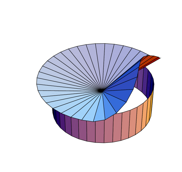
Figure 1: A Cone and a cylinder that are made by smooth deformations of a portion of a sheet without stretching. Both the cone and the cylinder are developable surfaces and the straight lines shown are generators for the surfaces. Note that the Cone has a singularity at its apex, where it has an infinite curvature.

We now consider a general isometric embedding of a $2$-disk in ${\mathbb{R}}^{3}$. We can choose global Cartesian co-ordinates on the disk and also on ${\mathbb{R}}^{3}$. In these co-ordinates, the embedding is given by three real-valued function $r^{a}(x^{\alpha}),a=1,2,3$, where $x^{\alpha},\alpha=1,2$ are Cartesian co-ordinates on the disk. If we let ${\mathbf{r}}(x^{\alpha})$ denote a vector valued function with components $r^{a}(x^{\alpha})$, the strain is given by landau

$$u_{\alpha\beta}=\frac{\partial{\mathbf{r}}}{\partial x^{\alpha}}\cdot\frac{\partial{\mathbf{r}}}{\partial x^{\alpha}}-\delta_{\alpha\beta}$$ (1)

and the curvature is given by

$$C_{\alpha\beta}=\frac{\partial^{2}{\mathbf{r}}}{\partial x^{\alpha}\partial x^{\beta}}\cdot{\mathbf{n}},$$ (2)

where $\mathbf{n}$ is the unit normal to the surface. The principal curvatures are the eigenvalues of the symmetric matrix $C_{\alpha\beta}$. The Gaussian curvature is defined as the product of the principal curvatures.

To show the existence of generators for all isometric immersions of a flat sheet in $\mathbb{R}^{3}$, we need Gauss’ Theorema Egregium DiffGeom2 . This theorem asserts that the isometric immersion yields a developable surface, so that the Gaussian curvature is zero everywhere. Consequently, at least one of the principal curvatures is zero at every point on the surface.

Let $p$ denote the center of the 2-disk that is embedded in ${\mathbb{R}}^{3}$. We first consider the case where only one principal curvature is zero at $p$. Since only one principal curvature is zero, there is a unique generator through $p$. It can be shown that this generator can be extended until it runs into the boundary of the disk at $q$. Since the image of the generator $pq$ in $\mathbb{R}^{3}$ is also a straight line, $d(p,q)=1$ implies that $r(p,q)=1$. Consequently, the sheet cannot be embedded inside a shell with a diameter less than $1$.

We now consider the remaining case: that both principal curvatures vanish at $p$. In this case, there isn’t a unique generator through $p$. Further, not every local generator through $p$ need be extendible as a straight line in the embedding space ($\mathbb{R}^{3}$) all the way to the boundary as is evident from Fig. 2. In this case, we pick a local generator and extend it as far as possible while keeping it a straight line in $\mathbb{R}^{3}$. Let the maximal straight line be $ps$. Both principal curvatures are zer o at the point $s$, but, given an $\epsilon>0$, we can find a point $p_{1}$ close to $s$ such that one principal curvature is non-zero at $p_{1}$ and $d(s,p_{1})<\epsilon$ (see Fig. 3). Since the point $p_{1}$ has one nonzero principal curvature, from the argument in the previous paragraph, it follows that there exists a point $s_{1}$ on the boundary such that the image of the geodesic $p_{1}s_{1}$ in the sheet is a straight line in $\mathbb{R}^{3}$. If the curvature is everywhere bounded, by making $d(s,s_{n})$ sufficiently small, we can make the angles between the segments $p_{1}s_{1}$ and $ps$ virtually the same in both the sheet and in the space so that $d(p,s_{1})-r(p,s_{1})$ is as small as we please.

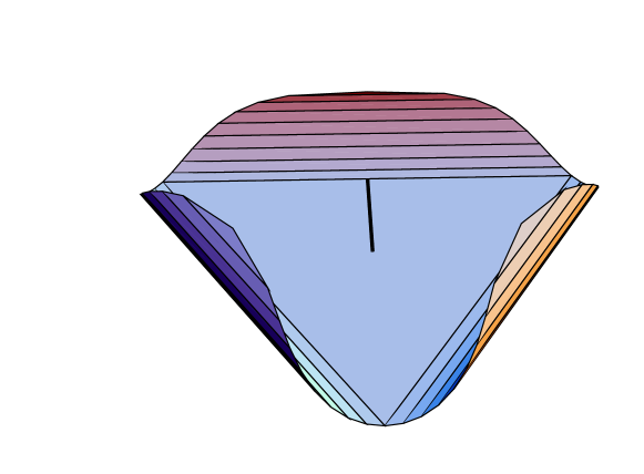
Figure 2: A disk with both principal curvatures zero at the center. The inner triangle is the region where both the principal curvatures are zero. The three curved regions have one non-zero principal curvature. The straight line are the generators of this surface. The thick line is a generator through the center that can not be extended till the boundary. The inner triangle is the set ${\cal A}_{1}={\cal B}_{1}$ and the three curved regions together are the set ${\cal B}_{0}$. The generators in the the curved regions are the leaves of the relative nullity distribution $\Delta$ in ${\cal B}_{0}$ and the inner triangle is a leaf of $\Delta$ in ${\cal B}_{1}$. (See Sec. III.2 for the definitions of ${\cal A}_{1},{\cal B}_{1},{\cal B}_{0},\Delta$ and “the leaves of a distribution”.)

We will now show this rigorously. The difference between $d(p,s_{1})$ and $r(p,s_{1})$ is due to two factors. One contributing factor is that the small segment $sp_{1}$ is flat in the sheet but curved in the embedding space, so that $r(s,p_{1})\neq d(s,p_{1})$. However, both these lengths are small, since they are bounded by $\epsilon$, and the contribution of this segment to $d(p,s_{1})-r(p,s_{1})$ is bounded by $2\epsilon$.

Another contributing factor is that, since the curvature is not zero on the segment $sp_{1}$, the angles between the straight segments $ps$ and $p_{1}s_{1}$ in the embedding space and in the sheet are not equal. Let $\theta$ denote the angle between the segments $ps$ and $p_{1}s_{1}$ in the sheet and let $\theta^{\prime}$ be the angle between the images of these segments in the embedding space. Since the curvature is a measure of the rate of change of the angle that a tangent vector makes with respect to a fixed axis, it is easily seen that

$$|\theta-\theta^{\prime}|\leq Kd(s,p_{1}),$$

where $K$ is a bound on the components of the curvature tensor ${\mathbf{K}}^{a}_{\alpha\beta}$. Since the segments $ps$ and $p_{1}s_{1}$ are straight both in the sheet and in the embedding space, $r(p,s)=d(p,s)$ and $r(p_{1},s_{1})=d(p_{1},s_{1})$. Also, $r(s,p_{1})\leq d(s,p_{1})\leq\epsilon$. Combining the estimates

$$|d(p,s_{1})-\sqrt{d(p,s)^{2}+d(p_{1},s_{1})^{2}-2d(p,s)d(p_{1},s_{1})\cos(\theta)}|\leq d(s,p_{1})\leq\epsilon,$$

$$|r(p,s_{1})-\sqrt{r(p,s)^{2}+r(p_{1},s_{1})^{2}-2r(p,s)r(p_{1},s_{1})\cos(\theta^{\prime})}|\leq r(s,p_{1})\leq\epsilon,$$

$$|\cos(\theta)-\cos(\theta^{\prime})|\leq|\theta-\theta^{\prime}|$$

with the results from above and using $d(p,s)\leq R,d(p_{1},s_{1})\leq R$, where $R$ is the radius of the disk, we obtain

$$|d(p,s_{1})-r(p,s_{1})|\leq C_{1}(2+KR)\epsilon$$

where $C_{1}>1$ is a constant. Note that the bound on the right hand side reflects the contributions of both the factors – the term $2\epsilon$ is the contribution from the length of the segment $sp_{1}$, and the term $KR\epsilon$ is the contribution from the difference between the angles $\theta$ and $\theta^{\prime}$.

Now, we choose a sequence $\delta_{n}\rightarrow 0$ and repeat this construction with $\epsilon=\delta_{n}$, for each $n$. This will yield a point $s_{1}(n)=q_{n}$ on the boundary with $r(p,q_{n})-d(p,q_{n})\leq C_{1}(2+KR)\delta_{n}$ so that $r(p,q_{n})-d(p,q_{n})\rightarrow 0$ as $n\rightarrow\infty$. Since the boundary of the unit disk is compact, the sequence $q_{n}$ has an accumulation point $q$ on the boundary and there exists a subsequence $q_{n_{k}}$ that converges to $q$. From the above estimate, it follows that $r(p,q)=d(p,q)$ and $d(p,q)=1$ implies that the disk cannot be isometrically embedded inside a spherical shell with a diameter less than $1$.

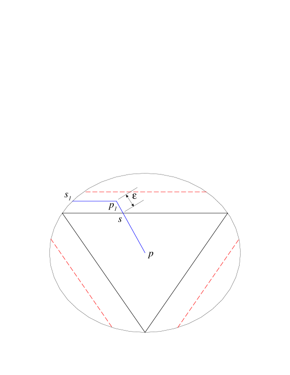
Figure 3: This figure is a 2-dimensional representation of the embedding in Fig. 2. The inner triangle is the region where both the principal curvatures are zero and the three sets bounded by a circular arc and an edge of the triangle are the regions with one non-zero principal curvature. The dashed lines represent the generators in these regions. The point $p$ is the center of the disk and $ps$ is a straight line through the center that cannot be extended keeping it straight in the embedding space. The point $p_{1}$ is in the curved region within $\epsilon$ of $s$. The point $s_{1}$ is the intersection of the generator through $p_{1}$ with the boundary of the disk.

Our generalization to an $m$-disk in a $d$-shell, presented in Sec. III, is along the same lines as the argument above for developable surfaces in $\mathbb{R}^{3}$. Now the local curvature is a vector-valued tensor rather than a scalar-valued tensor, so that there are no obvious “principal curvatures” and no obvious generalization of the Gaussian curvature. Nevertheless, we will show that there are analogs of the local generators. In the situation $d<2m$, Lemma 1 along with Corollary 1.1 asserts that there exists at least one line through the point $p$ in the $m$-sheet that has zero curvature in the embedding space at $p$. The direction of this line is a local “flat direction” at $p$.

Lemmas 2, 3 and 4 show that there exists a “large” set of points ${\cal U}$ such that –

1. Almost every point in the sheet is in ${\cal U}$.

2. If $p\in{\cal U}$, it is possible to extend the line that has zero curvature locally to get a straight line of finite length that is also a geodesic in the embedding space.

Given a point $p_{0}\in{\cal U}$, there exists a maximal extension of a zero curvature line through $p_{0}$, and we will denote the other endpoint of this segment by $s_{0}$. Therefore, $s_{0}$ has the property that it is not possible to extend $p_{0}s_{0}$ any further while keeping it a geodesic in the embedding space. Lemma 4 also tells us that the number of flat directions is a constant along a geodesic so that it is the same at $s_{0}$ and $p_{0}$.

Given any $\epsilon>0$, Lemma 5 asserts the existence of a point $p_{1}$ in ${\cal U}$ such that $d(s_{0},p_{1})<\epsilon$ and the number of local flat directions at $p_{1}$ is less than the number of flat directions at $s_{0}$. Since $p_{1}\in{\cal U}$, we can now start from $p_{1}$ and proceed along a maximally extended geodesic until its termination point $s_{1}$. Repeating this process, we get sequences of points $p_{2},p_{3},\ldots,p_{k}$ and $s_{1},s_{2},\ldots,s_{k}$ such that

1. The image of the straight line $p_{j}s_{j}$ is a geodesic in the embedding space.

2. $p_{j+1}$ has fewer local flat directions than $p_{j}$, and

3. $d(s_{j},p_{j+1})<\epsilon$.

Since the number of flat directions is between $1$ and $m$ everywhere on the sheet, it follows that the sequences $p_{j}$ and $s_{j}$ are finite. Consequently, for some finite $k$, the point $s_{k}=q$ lies on the boundary of the disk.

Lemma 6 shows that for the image of a straight line $pq$ in the sheet to be a geodesic in the embedding space, it is necessary and sufficient that $r(p,q)=d(p,q)$. It follows that $r(p_{j},s_{j})=d(p_{j},s_{j})$ for all $j$. Lemma 7 shows that if $r(p,p_{1})=d(p,p_{1})$ and $r(p_{1},p_{2})=d(p_{1},p_{2})$ , then $r(p,p_{2})=d(p,p_{2})$. That is, if two points $p$ and $q$ can be connected by a curve that is a piecewise geodesic in the embedding space, the image of the straight line connecting $p$ and $q$ in the sheet is also a geodesic in the embedding space.

By taking a sequence $\delta_{n}\rightarrow 0$, we can repeat the above construction for each $n$ with $\epsilon=\delta_{n}$. This will yield a sequence of points $q_{n}$ on the boundary such that $p$ can be connected to $q_{n}$ by a discontinuous, piecewise straight curve, with a finite number of straight line segments $p_{j}s_{j}$. The discontinuities go to zero as $n$ goes to infinity since $d(s_{j},p_{j+1})<\delta_{n}$. The compactness of the boundary of the disk, gives an accumulation point $q$ for the sequence $q_{n}$. The above construction along with Lemma 6 and Lemma 7 show that, given any point $p$ in the disk, there exists a point $q$ on the boundary of the disk such that $r(p,q)=d(p,q)$. Since $d(p,q)=1$ when $p$ is the center of the disk, it follows that the disk cannot be embedded in a ball with diameter less than 1.

III The geometry of a confined $m$-sheet

We will consider the problem of the existence of an isometry $\phi:D^{m}\rightarrow\bar{B}_{r}$. In Sec. III.1, we will set up the notation we use and review the differential geometry of isometric immersions. In Sec. III.2, we prove the results stated in Sec. II.

III.1 Review of Differential Geometry

In this section, we will review the differential geometry of the isometric immersion of $m$-manifolds in $d$-manifolds. We will use the co-ordinate (index) free language and follow the presentation in Ref. daj , but we will restate our results in the indexed notation where appropriate.

We will consider the case of a smooth $m$-manifold $M$, typically the unit disk in $m$ dimensional Euclidean space, immersed in a smooth $d$-manifold $\tilde{M}$, typically $R^{d}$. Since both $M$ and $\tilde{M}$ are subsets of Euclidean spaces, we can find global Cartesian co-ordinates (a co-ordinate patch that covers the entire manifold) for both $M$ and $\tilde{M}$. We will denote these co-ordinates on $M$ by $x^{\alpha}$ (greek superscripts) and on $\tilde{M}$ by $r^{a}$ (roman superscripts).

We will require that the immersion $\phi:M\rightarrow\tilde{M}$ be smooth. Here, $\phi$ is the co-ordinate free representation of the immersion given by the $d$ functions $r^{a}(x^{\alpha}),a=1,2,\ldots,d$. Let $TM$ and $T\tilde{M}$ denote the tangent bundles of $M$ and $\tilde{M}$ respectively. We will use $(\psi)^{a}$ with a roman superscript to denote the indexed representation of a quantity $\psi$ that takes values in $\tilde{M}$ or $T\tilde{M}$ and $(U)^{\alpha}$ with a greek superscript to denote the indexed representations of a quantity $U$ that take values in $M$ or $TM$. Using this notation, the statement that $\phi(x)$ is the index free representation of $r^{a}(x^{\alpha})$ is written as $(\phi)^{a}((x)^{\alpha})=r^{a}(x^{\alpha})$.

The immersion induces a map $\phi_{*}(x):T_{x}M\rightarrow T_{\phi(x)}\tilde{M}$ between the tangent space of $M$ at $x$ and the tangent space of $\tilde{M}$ at $\phi(p)$ that is injective (one to one) for each $x\in M$. Since the immersion $\phi$ is isometric,

$$\langle\phi_{*}X,\phi_{*}Y\rangle_{\tilde{M}}=\langle X,Y\rangle_{M},$$

for every $x\in M$ and $X,Y\in T_{x}M$, $\langle.,.\rangle_{M}$ denotes the Riemannian metric on $M$ and similarly for $\tilde{M}$. For the case $\phi:D^{m}\rightarrow\mathbb{R}^{d}$ that we are considering, since the $x^{\alpha}$ are global Cartesian co-ordinates, the metric on $D^{m}$ is given by $\langle X,Y\rangle_{M}=\delta_{\alpha\beta}(X)^{\alpha}(Y)^{\beta}$, and the immersion is given by a vector valued function $\mathbf{r}(x^{\alpha})$ with Cartesian components $r^{a}(x^{\alpha})$. The above equation is then equivalent to the statement

$$\partial_{\alpha}\mathbf{r}\cdot\partial_{\beta}\mathbf{r}=\delta_{\alpha\beta}.$$

We are therefore asserting that the strain $u_{\alpha\beta}$ is identically zero.

Locally identifying $M$ with its image under $\phi$, we can consider the tangent space of $M$ at $x$ as a subspace of the tangent space of $\tilde{M}$. Because of this identification, we will henceforth denote the vector $\phi_{*}X\in T\tilde{M}$ by $X$ for all $X\in TM$. For each point $x\in M$, we will denote the subspace of vectors in $T_{\phi(x)}\tilde{M}$ that are orthogonal to the vector $X=\phi_{*}X\in T\tilde{M}$ for all $X\in TM$ by $T_{x}M^{\perp}$. This gives the decomposition

$$T_{\phi(x)}\tilde{M}=T_{x}M\oplus T_{x}M^{\perp},$$

where $T_{x}M^{\perp}$ is the orthogonal complement of $T_{x}M$ in $T_{\phi(x)}\tilde{M}$. The vector bundle

$$TM^{\perp}=\bigcup_{x\in M}T_{x}M^{\perp},$$

is called the normal bundle to $M$. Therefore, the union of the tangent spaces $T_{y}\tilde{M}$ over all the points in $y\in\tilde{M}$ that are in the image $\phi(M)$, is the vector bundle given by

$$\left.T\tilde{M}\right|_{\phi(M)}=\bigcup_{x\in M}\left(T_{x}M\oplus T_{x}M^{\perp}\right).$$

This will motivate defining the tangential projection

$$()^{T}:\left.T\tilde{M}\right|_{\phi(M)}\rightarrow TM,$$

and the normal projection

$$()^{\perp}:\left.T\tilde{M}\right|_{\phi(M)}\rightarrow TM^{\perp}.$$

As explained in the Appendix, there exists a differential operator on a Riemannian manifold, called the Levi-Civita connection waldbook .The connections on $\tilde{M}$ and $M$ are related by the Gauss Formula:

$$\tilde{\nabla}_{X}Y=(\tilde{\nabla}_{X}Y)^{T}+(\tilde{\nabla}_{X}Y)^{\perp}=\nabla_{X}Y+\alpha(X,Y),$$ (3)

where $X,Y\in TM$ are arbitrary (smooth) vector fields and $\alpha:TM\times TM\rightarrow TM^{\perp}$ is a symmetric bilinear map. $\alpha$ is called the second fundamental form of $\phi$. A calculation using the representation $r^{a}(x^{\alpha})$ for the immersion $\phi$ shows that

$$(\alpha(X,Y))^{a}=K^{a}_{\alpha\beta}(X)^{\alpha}(Y)^{\beta}.$$

$\alpha$ is therefore the co–ordinate free representation of the extrinsic curvature ${\mathbf{K}}_{\alpha\beta}$ (See Eq. (2)).

Given vector fields $X\in TM$ and $\xi\in TM^{\perp}$, the shape operator $A_{\xi}:TM\rightarrow TM$ is defined by

$$A_{\xi}X=-(\tilde{\nabla}_{X}\xi)^{T}.$$

Using $\langle\xi,Y\rangle=0$ for every vector field $Y\in TM$ and computing $\tilde{\nabla}_{X}\langle\xi,Y\rangle$ yields

$$\langle A_{\xi}X,Y\rangle=\langle\alpha(X,Y),\xi\rangle.$$

We denote the normal component of $\tilde{\nabla}_{X}\xi$ by $\nabla^{\perp}_{X}\xi$ and this defines a compatible connection on the normal bundle. The above equation yields the Weingarten Formula

$$\tilde{\nabla}_{X}\xi=-A_{\xi}X+\nabla_{X}^{\perp}\xi.$$ (4)

A characterization of the intrinsic geometry of a manifold is given by the Riemann Curvature manifolds ; waldbook –

Definition 2.

For a Riemannian manifold $M$ with a Levi-Civita connection $\nabla$, the Riemann (or Intrinsic) curvature tensor $R$ is given by

$$R(X,Y)Z=\nabla_{X}\nabla_{Y}Z-\nabla_{Y}\nabla_{X}Z-\nabla_{[X,Y]}Z$$

where $X,Y,Z\in TM$ are arbitrary (smooth) vector fields and the Lie-Product $[.,.]$ is defined by

$$[X,Y]=\nabla_{X}Y-\nabla_{Y}X.$$

Remark 1.

The Riemann curvature is zero for the Euclidean space ${\mathbb{R}}^{m}$. It can be shown that the Riemann curvature is also zero for all manifolds that are isometric embeddings of ${\mathbb{R}}^{m}$ in a larger space. The converse is also true, so that the Riemann curvature of an $m$-manifold $M$ being zero implies that given $q\in M$ there is an open set $U\in M$ containing $q$ such that there exists an isometry $\phi:V\rightarrow U$, where $V$ is an open neighborhood of the origin in ${\mathbb{R}}^{m}$.

Computing the curvature tensor of $\tilde{M}$ and taking the tangential projection of $\tilde{R}(X,Y)Z$ yields the Gauss Equation

$$\langle R(X,Y)Z,W\rangle=\langle\tilde{R}(X,Y)Z,W\rangle+\langle\alpha(X,W),\alpha(Y,Z)\rangle-\langle\alpha(X,Z),\alpha(Y,W)\rangle,$$ (5)

where $R$ and $\tilde{R}$ are the curvature tensors of $M$ and $\tilde{M}$ respectively. Taking the normal projection gives the Codazzi Equation

$$(\tilde{R}(X,Y)Z)^{\perp}=(\nabla^{\perp}_{X}\alpha)(Y,Z)-(\nabla^{\perp}_{Y}\alpha)(X,Z),$$ (6)

where

$$(\nabla^{\perp}_{X}\alpha)(Y,Z)=\nabla^{\perp}_{X}(\alpha(Y,Z))-\alpha(\nabla_{X}Y,Z)-\alpha(Y,\nabla_{X}Z).$$

Definition 3.

A subspace valued function, that is a function defined on a manifold $M$, whose value at a point $x\in M$ is a subspace of $T_{x}M$ is called a distribution.

Given an isometric immersion $\phi:M\rightarrow\tilde{M}$, the second fundamental form $\alpha:TM\times TM\rightarrow TM^{\perp}$ determines a distribution as follows. For each $x\in M$, a subspace $\Delta(x)$ is defined by

$$\Delta(x)=\{p\in T_{x}M:\alpha(Y,p)=0\mbox{ for all }Y\in T_{x}M\}.$$

$\Delta(x)$ is called the subspace of relative nullity and its dimensionality is the index of relative nullity $\nu(x)$. The relative nullity distribution $\Delta$ is the function $x\mapsto\Delta(x)$, the subspace of relative nullity at $x$.

Definition 4.

A distribution $D$ is smooth on a set $U\subseteq M$ if there exist smooth vector fields $X_{i}:U\rightarrow TU,i=1,2,\ldots,p$ such that at each $x\in U$, the vectors $X_{i}(x)\in TU,i=1,2,\ldots,p$ form a basis for the subspace $D(x)$.

III.2 Immersion Theorems

We will now restrict our attention to smooth isometric mappings $\phi:D^{m}\rightarrow\mathbb{R}^{d}$, where $D^{m}=\{\mathbf{x}\in\mathbb{R}^{m}:\|\mathbf{x}\|\leq 1\}$ is the closed unit disk in $\mathbb{R}^{m}$, and both $D^{m}$ and $\mathbb{R}^{d}$ are equipped with the standard Euclidean metric. In this case, both $D^{m}$ and ${\mathbb{R}}^{d}$ have zero Riemann curvature, so that, for the isometric immersion $\phi$, the Gauss equation (5) yields

$$\langle\alpha(X,W),\alpha(Y,Z)\rangle-\langle\alpha(X,Z),\alpha(Y,W)\rangle=0$$ (7)

and the Codazzi equation (6) yields

$$(\nabla^{\perp}_{X}\alpha)(Y,Z)-(\nabla^{\perp}_{Y}\alpha)(X,Z)=0,$$ (8)

for arbitrary $X,Y,Z,W\in TD^{m}$.

We will define $\rho(\phi)$, the span or the diameter of the immersion $\phi$ as

$$\rho(\phi)=\sup_{\mathbf{x},\mathbf{y}\in D^{m}}r({\mathbf{x}},\mathbf{y}),$$

where

$$r({\mathbf{x}},\mathbf{y})=\|\phi(\mathbf{x}),\phi(\mathbf{y})\|_{\mathbb{R}^{d}},$$

is the Euclidean distance between the images of the points $\mathbf{x}$ and $\mathbf{y}$ in $\mathbb{R}^{d}$. We will denote the Euclidean distance in $D^{m}\subset R^{m}$ between the points ${\mathbf{x}}$ and $\mathbf{y}$ by $d(\mathbf{x},\mathbf{y})$.

Using this definition of the span of an embedding, we can reformulate the question about the existence of an isometry $\phi:D^{m}\rightarrow\bar{B}_{r}$ for arbitrary $r>0$ (See Sec. II) as follows – Given any $R_{s}$ with $0<R_{s}<1$, Is there a smooth isometric immersion $\phi:D^{m}\rightarrow\mathbb{R}^{d}$, with $\rho(\phi)\leq R_{s}$?

We first recall the earlier result Kramer.PRL on the existence of such an isometry for all $R_{s}>0$ if $d\geq 2m$.

Theorem 1.

If $d\geq 2m$, there exists a smooth isometry $\phi$ with $\rho(\phi)\leq R_{s}$, for any given $R_{s}$, $0<R_{s}<1$.

Proof.

This proof is from Ref. Kramer.PRL . Define

$$\phi:(x_{1},x_{2},\ldots,x_{m})\rightarrow(y_{1},y_{2},\ldots,y_{2m},\ldots y_{n}),$$

by

$$y_{2i-1}=\frac{R_{s}}{\sqrt{2m}}\cos\left(\frac{\sqrt{2m}x_{i}}{R_{s}}\right),y_{2i}=\frac{R_{s}}{\sqrt{2m}}\sin\left(\frac{\sqrt{2m}x_{i}}{R_{s}}\right),$$

for $i=1,2,\ldots m$, and

$$y_{k}=0,$$

for $k>2m$. Clearly $\rho(\phi)\leq R_{s}$. Computing the strain $u_{\alpha\beta}$ by Eq. (1) gives $u_{\alpha\beta}=0$ showing that $\phi$ is a smooth isometry with $\rho(\phi)\leq R_{s}$. ∎

The following theorem is the main result of this paper –

Theorem 2.

If $d<2m$, and $\phi:D^{m}\rightarrow\mathbb{R}^{d}$ is a smooth isometric immersion, $\rho(\phi)\geq 1$.

This theorem implies the nonexistence of a smooth isometric immersion $\phi$ with $\rho(\phi)<R_{s}$ for arbitrarily small but positive $R_{s}$. Before we prove this theorem, we will prove a few results that are useful in the proof of the theorem.

Definition 5.

Let $V$ and $U$ be finite dimensional vector spaces and $\beta:V\times V\rightarrow U$ be a bilinear map. We denote by $N(\beta)$ the subspace

$$N(\beta)=\{n\in V:\beta(Y,n)=0,\mbox{for all }Y\in V\}$$

called the (right) kernel of $\beta$. We may define, similarly the left kernel. If $\beta$ is symmetric, the left and the right kernels agree and the subspace $N(\beta)$ is called the kernel of $\beta$.

Definition 6.

Let $V$ and $U$ be finite dimensional vector spaces. A bilinear map $\beta:V\times V\rightarrow U$ is flat with respect to a non-degenerate inner product $\langle.,.\rangle:U\times U\rightarrow\mathbb{R}$ if

$$\langle\beta(X,W),\beta(Y,Z)\rangle-\langle\beta(X,Z),\beta(Y,W)\rangle=0$$

for all $X,Y,Z,W\in V$.

Lemma 1.

Let $\beta:V\times V\rightarrow U$ be a symmetric flat bilinear form with respect to the positive definite inner product $\langle.,.\rangle:U\times U\rightarrow\mathbb{R}$. Then

$$\dim N(\beta)\geq\dim V-\dim U.$$

This result and the corollary that follows (Corollary 1.1) are due to E. Cartan cartan .

Proof.

Setting $W=X$ and $Z=Y$ in the definition of a flat bilinear form and using the symmetry of $\beta$ gives

$$\langle\beta(X,X),\beta(Y,Y)\rangle=\langle\beta(X,Y),\beta(X,Y)\rangle\hskip 60.0pt(*)$$

for every $X,Y\in V$. We will use this result repeatedly in the proof of the lemma.

Let $\dim V=m$ and $\dim U=k$. We need to demonstrate the existence of at least $m-k$ linearly independent vectors $n_{1},n_{2},\ldots,n_{m-k}$ such that $\beta(n_{i},Y)=0$ for all $Y\in V$ and $i=1,2,\ldots,m-k$.

We only need to consider the case $m>k$ as there is nothing to prove for $m\leq k$. It suffices to demonstrate the existence of a single $p\neq 0$ satisfying $\beta(Y,p)=0$ for all $Y\in V$. To see this, note that, having found one such $p$, $\beta$ naturally induces a map $\beta_{1}:V/V_{1}\times V/V_{1}\rightarrow U$ where $V_{1}$ is the subspace spanned by $p$ so that $V/V_{1}$ is a vector space of dimension $m-1$ and then repeat the demonstration of the existence of a vector $p_{1}\in V/V_{1}$. Continue in this way, reducing the dimension of the quotient by one at each step, until that dimension has been reduced to $k$. In fact, it suffices to find a nonzero $p$ satisfying $\beta(p,p)=0$, for this automatically implies $\beta(Y,p)=0$ for all $Y\in V$ by $(*)$ and the positive-definiteness of $\langle Z,Z\rangle$.

To exhibit a suitable $p$, we first construct a maximal set of non-zero vectors $p_{1},p_{2},\ldots,p_{l}$ such that $\beta(p_{i},p_{j})=0$ for $i\neq j$. We will construct this set inductively. Let $p_{1},\cdots,p_{s}$ be a set of $s$ elements of $V$, such that $\beta(p_{i},p_{j})=0$ for $i,j=1,\cdots,s;\ i\neq j$. Such a set always exists since we can choose $s=1$ and set $p_{1}$ to be any non-zero vector in $V$. This set can be enlarged since we can show the existence of an $(s+1)$th vector, $p_{s+1}$, such that the above holds for $i,j=1,\cdots,(s+1);\ i\neq j$. To this end, set $v=p_{1}+\cdots+p_{s}$. Choose any $q\neq 0$ in $V$ with $\beta(q,v)=0$. This is always possible, since $\dim V>\dim U$, and to find such a $q$, we need to solve $k$ linear equations in $m>k$ unknowns. Then $(*)$, with $X=q$, $Y=v$, yields

$$0=\langle\beta(q,q),\beta(v,v)\rangle=\langle\beta(q,q),(\sum\beta(p_{i},p_{i})),\rangle$$

where, we have used the bilinearity of $\beta(.,.)$ and $\langle.,.\rangle$. But for each $i$, we have

$$\langle\beta(q,q),\beta(p_{i},p_{i})\rangle=\|\beta(q,p_{i})\|^{2}\geq 0,$$

by $(*)$ and the positive-definiteness of $\langle.,.\rangle$. It follows that $\beta(q,p_{i})=0$ for all $i=1,\cdots,s$. So, $p_{s+1}=q$ is the desired vector.

Using $(m+1)$ times the result of the paragraph above, construct nonzero vectors $p_{1},\cdots,p_{m+1}$, with $\beta(p_{i},p_{j})=0$, for $i,j=1,\cdots,(m+1);\ i\neq j$. These must be dependent, i.e., we must have $\sum r_{i}p_{i}=0$, with at least one $r_{i}$, say $r_{n}$, nonzero. But now we have $0=\beta(p_{n},\sum r_{i}p_{i})=r_{n}\beta(p_{n},p_{n})$. We conclude that $\beta(p_{n},p_{n})=0$. Setting $p=p_{n}$ gives the existence of a $p$ such that $\beta(p,p)=0$ and as remarked above, this suffices to prove the lemma.

∎

Let $\phi:D^{m}\rightarrow\mathbb{R}^{d}$ be a smooth isometric immersion. The second fundamental form $\alpha$ of the immersion $\phi$ at is a symmetric bilinear map $\alpha:TM\times TM\rightarrow TM^{\perp}$. Eq. (7) implies that $\alpha$ is a flat bilinear form. At each point $\mathbf{x}\in D^{m}$, where $TM_{\mathbf{x}}$ is a vector space with dimension $m$ and $TM^{\perp}_{\mathbf{x}}$ is a vector space with dimension $d-m$. Also, the Kernel $N(\alpha_{\mathbf{x}})$, is the subspace of relative nullity $\Delta(\mathbf{x})$. Therefore, Lemma 1 yields the following corollary:

Corollary 1.1.

Let $\phi:D^{m}\rightarrow\mathbb{R}^{d}$ be a smooth, isometric immersion. Then, for all $\mathbf{x}\in D^{m}$, the index of relative nullity $\nu(\mathbf{x})\geq 2m-d$.

We denote by $\nu_{0}$ the index of minimum relative nullity of $\phi$ given by

$$\nu_{0}=\min_{\mathbf{x}\in D^{m}}\nu(\mathbf{x}).$$

By Corollary 1.1, we have that $\nu_{0}\geq 2m-d$. We are considering the case $d<2m$ so that $\nu_{0}\geq 1$.

Definition 7.

The indices of relative nullity at various points in $D^{m}$ can be arranged in an increasing sequence $\nu_{0}<\nu_{1}<\ldots<\nu_{k}$. Clearly, this is a finite sequence since $\nu_{k}\leq m$. We define the sets $D^{m}={\cal A}_{0}\supseteq{\cal A}_{1}\supseteq\ldots\supseteq{\cal A}_{k}$, by

$${\cal A}_{j}=\{\mathbf{x}\in D^{m}:\nu(\mathbf{x})\geq\nu_{j}\}$$

for $j=0,1,\ldots,k$. We also define the sets ${\cal B}_{0},{\cal B}_{1},\ldots,{\cal B}_{k}$ by

$${\cal B}_{j}=\{\mathbf{x}\in D^{m}:\nu(\mathbf{x})=\nu_{j}\}={\cal A}_{j}-{\cal A}_{j+1}$$

for $j=0,1,\ldots,k$ with the convention ${\cal A}_{k+1}$ is the empty set $\emptyset$.

Recall that a distribution is a subspace valued function on $M$. We will now prove some results about the relative nullity distribution $\Delta$ that is given by ${\mathbf{x}}\mapsto\Delta({\mathbf{x}})$.

Lemma 2.

For an isometric immersion $\phi:M\rightarrow\tilde{M}$, we have :

1. The relative nullity distribution $\Delta$ is smooth on any open set $U$ where $\nu$ is a constant,

2. The set ${\cal B}_{j}$ is open in ${\cal A}_{j}$, so that, if ${\mathbf{x}}\in{\cal B}_{j}$, there is an open neighborhood ${\cal N}$ of ${\mathbf{x}}$ such that $\nu$ is a constant on ${\cal N}\cap{\cal A}_{j}$.

A closely related result is proved in Dajczer daj (Prop. 5.2). The proof presented below is essentially the same as the proof in daj .

Proof.

1. Set $m=\dim M$. Let $\dim\Delta(\mathbf{x})=\nu(\mathbf{x})=p$ for all points in the open subset $U$. Let $\Delta^{\perp}(\mathbf{x})$ be the orthogonal complement of $\Delta(\mathbf{x})$ in $T_{\mathbf{x}}M$. Evidently the dimension of $\Delta^{\perp}$ is $m-p$. On the other hand, we may express $\Delta^{\perp}$ via

   $$\Delta^{\perp}(\mathbf{x})=\mathrm{span}\left\{A_{\xi}X:\mbox{ for all }X\in T_{\mathbf{x}}M,\xi\in T^{\perp}_{\mathbf{x}}M\right\},$$

   given $\mathbf{x}_{0}\in U$, there exist $X_{1},X_{2},\ldots,X_{m-p}\in TM_{\mathbf{x}_{0}}$ and $\xi_{1},\ldots,\xi_{m-p}\in TM^{\perp}_{\mathbf{x}_{0}}$ ,such that

   $$\Delta^{\perp}(\mathbf{x})=\mathrm{span}\left\{A_{\xi_{j}}X_{j}\right\},$$

   Take smooth local extensions $X_{1},\ldots,X_{m-p}\in TM$ and $\xi_{1},\ldots,\xi_{m-p}\in TM^{\perp}$. Clearly,

   $$\mathrm{span}\left\{A_{\xi_{j}}X_{j}\right\}\subseteq\Delta^{\perp}.$$

   By continuity, the vector fields $A_{\xi_{j}}X_{j}$ are linearly independent in a neighborhood of $\mathbf{x}_{0}$. $U$ is open so that we can choose this neighborhood in such a way that $\dim\Delta^{\perp}=m-\nu(\mathbf{x})=m-p$. Therefore, in this neighborhood

   $$\Delta^{\perp}=\mathrm{span}\left\{A_{\xi_{j}}X_{j}\right\}.$$

   This implies that $\Delta^{\perp}$ is a smooth distribution on $U$ and consequently, so is $\Delta$.

2. follows immediately from the above argument by noting that the set ${\cal A}_{j}$ is the set of all $\mathbf{x}$ with $\nu(\mathbf{x})\geq\nu_{j}$.

∎

Corollary 2.1.

The sets ${\cal A}_{j}$ for $j=1,\ldots,k$ are all closed in $D^{m}$ by Lemma 2.

Remark 2.

To clarify the relationships between these closed and open sets, we consider the 3-cornered shape of Fig. 2. In this example, $k=1$, $\nu_{0}=1$ and $\nu_{1}=\nu_{k}=2$. The set ${\cal A}_{0}$ is the whole disk, and ${\cal A}_{1}$ is the flat triangular region in the middle. The set ${\cal B}_{0}$ consists of the three curved side regions, while ${\cal B}_{1}$ is the same as ${\cal A}_{1}$. Evidently ${\cal B}_{1}$ is open in ${\cal A}_{1}$, since the two sets are the same. Any neighborhood of a point in ${\cal B}_{1}$ that fails to be be in ${\cal B}_{1}$ clearly fails to be in ${\cal A}_{1}$ as well. On the other hand, ${\cal A}_{1}$ is not open in the whole disk and this implies that ${\cal B}_{1}$ is not open in the disk either.

Thus e.g., following any straight line from the flat region into the curved region, there is an identifiable last flat point with $\nu=2$. Turning to ${\cal B}_{0}$, it is open in ${\cal A}_{0}$, which is the whole disk. This means that if we traverse our line from the curved region into the flat region, there is no last point with $\nu=1$. These statements give the essential content of Lemma 2 and Corollary 2.1 for this example.

As we saw above, though ${\cal B}_{j}$ is open in ${\cal A}_{j}$, it is not necessarily open in $\mathbb{R}^{m}$. As evident from Lemma 2, it will be useful to look at open sets in $\mathbb{R}^{m}$ that have a constant index of relative nullity. For later purposes, it will also be important that the union of these open sets be ”large”, in the sense that given any point $p$ in $D^{m}$, we can find a sequence of points from these sets that converges to $p$. The following lemma gives the existence of such sets –

Lemma 3.

$\phi:D^{m}\rightarrow\mathbb{R}^{d}$ is an isometric immersion, and $d<2m$. Then, we have an open (in $\mathbb{R}^{m}$) set ${\cal U}$ that is dense in $D^{m}$ such that

$${\cal U}=\bigcup_{j=0}^{k}{\cal O}_{j}$$

where ${\cal O}_{j}$ for $j=0,1,2,\ldots,k$ is possibly empty, is open in $\mathbb{R}^{m}$, and is a subset of ${\cal B}_{j}$.

Proof.

Given a set $G\in\mathbb{R}^{m}$, let $\partial G$ denote the boundary of $G$, $\bar{G}$ denote the closure of $G$ and $G^{0}$ denote the interior of $G$.

First, we note that $A\subseteq D^{m}$ is closed in $\mathbb{R}^{m}$ implies that $\partial A$ is nowhere dense. This can be shown as follows:

Since $A$ is closed, $\partial A\subseteq A$. Therefore, $(\partial A)^{0}\subseteq A^{0}$. However, $\partial A=\bar{A}-A^{0}=A-A^{0}$. Consequently, it follows that $(\partial A)^{0}=\emptyset$.

Define ${\cal U}$ as

$${\cal U}=(D^{m})^{0}-\bigcup_{j=0}^{k}\partial{\cal A}_{j}=D^{m}-\partial D^{m}-\bigcup_{j=0}^{k}\partial{\cal A}_{j}$$

Clearly, ${\cal U}$ is open. $D^{m}$ is a closed subset of $\mathbb{R}^{m}$ with a nonempty interior, so that it is a second category set. Corollary 2.1 implies that each ${\cal A}_{j}$ is closed in $\mathbb{R}^{m}$. Therefore, the preceding argument along with the Baire category theorem implies that ${\cal U}$ is dense in $D^{m}$.

Now, we set ${\cal O}_{j}={\cal U}\cap{\cal B}_{j}$. Clearly, ${\cal O}_{j}\subseteq{\cal B}_{j}$. Also,

$$\bigcup_{j=0}^{k}{\cal B}_{j}=D^{m},$$

implies that

$$\bigcup_{j=0}^{k}{\cal O}_{j}={\cal U}.$$

Assume that ${\cal O}_{p}$ is nonempty and let $q\in{\cal O}_{p}$ be an arbitrary point. Then, $q\in{\cal B}_{p}$. Therefore, $q\in{\cal A}_{p}-{\cal A}_{p+1}={\cal A}_{p}\cap{\cal A}_{p+1}^{C}$, where ${\cal A}_{p+1}^{C}$ is the complement of ${\cal A}_{p+1}$ and is open in $\mathbb{R}^{m}$. From the definition of ${\cal U}$, it is clear that $q\notin\partial{\cal A}_{p}$. Since ${\cal A}_{p}$ is closed, ${\cal A}_{p}^{0}={\cal A}_{p}-\partial{\cal A}_{p}$. Therefore, we have

$$q\in{\cal A}_{p}^{0}\cap{\cal A}_{p+1}^{C}\cap{\cal U}\subseteq{\cal B}_{p}\cap{\cal U}={\cal O}_{p}.$$

This implies that $q$ is an interior point since ${\cal A}_{p}^{0}\,\cap\,{\cal A}_{p+1}^{C}\,\cap\,{\cal U}$ is an intersection of open sets, which gives an open neighborhood of $q$ contained in ${\cal O}_{p}$. Since $q$ was an arbitrary point in ${\cal O}_{p}$, it follows that every point in ${\cal O}_{p}$ is an interior point so that ${\cal O}_{p}$ is open. ∎

Observation 1.

Note that, in the above proof, we are not guaranteed the existence a point in ${\cal O}_{j}$ for a given $j$, so that ${\cal O}_{j}$ could be empty for some $j$. It can not be empty for all $j$ because ${\cal U}$, which is the union of the sets ${\cal O}_{j}$ over $j=1,2,\ldots,k$ is dense in $D^{m}$.

By definition, ${\cal A}_{0}=D^{m}$ and ${\cal B}_{0}\neq\emptyset$. By Lemma 2, ${\cal B}_{0}=B\cap D^{m}$ for some $B$ open in $\mathbb{R}^{m}$. Let $q\in B\cap D^{m}$. Since $B$ is open, it follows that there is an open neighborhood ${\cal N}$ of $q$ in $B$. It is also clear that, for any $q\in D^{m}$, ${\cal N}$ is an open neighborhood of $q$ implies that ${\cal N}\cap(D^{m})^{0}\neq\emptyset$. Clearly, ${\cal N}\cap(D^{m})^{0}\subseteq{\cal O}_{0}$, which is consequently non empty.

Recall that a distribution $D$ of index $p$ defined on an open subset $U\subset M$ is smooth if we can find a basis $X_{1}({\mathbf{x}}),X_{2}({\mathbf{x}}),\ldots,X_{p}({\mathbf{x}})$ for $R({\mathbf{x}})$ at each point ${\mathbf{x}}\in U$ such that the basis vectors $X_{1},X_{2},\ldots,X_{p}$ vary smoothly with ${\mathbf{x}}$.

Definition 8.

A smooth distribution $D$ defined on a set $U\subset{\mathbb{R}}^{m}$ with index $p$ is said to possess integral submanifolds (be completely integrable) if there exists a $m-p$ parameter family of $p$ dimensional embedded submanifolds of $U$ such that every point ${\mathbf{x}}\in U$ is contained in exactly one of these submanifolds and the tangent space of this submanifold coincides with $R({\mathbf{x}})$.

The integral submanifolds for a distribution $D$ are called the leaves of $D$.

Remark 3.

For the embedding represented in Fig. 2, the generators in ${\cal B}_{0}$ (the regions with one non-zero curvature) restricted to the interior of the disk are leaves of the relative nullity distribution $\Delta$. Similarly, the interior of the entire inner triangle is a leaf of $\Delta$ in ${\cal O}_{1}$.

Definition 9.

Let $U\subseteq M$ be an open set and let $X_{1},X_{2},\ldots,X_{p}$ be a set of smooth vector fields on $U$. The distribution $D$ given by

$${\mathbf{x}}\mapsto\mathrm{Span}(X_{1}({\mathbf{x}}),X_{2}({\mathbf{x}}),\ldots,X_{p}({\mathbf{x}}))$$

is said to be involutive, if at every ${\mathbf{x}}\in U$, the Lie-Product $[X_{i},X_{j}]({\mathbf{x}})\in R({\mathbf{x}})$ for all $1\leq i,j\leq p$.

A necessary and sufficient condition for a smooth distribution to be completely integrable is given by Frobenius’ theorem waldbook which states that a smooth distribution is integrable if and only if it is involutive.

Definition 10.

Let $M$ be a Riemannian manifold. A geodesic $\gamma:[a,b]\rightarrow M$ is a differentiable curve that is a stationary point for the functional

$$L[\gamma]=\int_{a}^{b}\sqrt{\langle\gamma^{\prime}(t),\gamma^{\prime}(t)\rangle_{\gamma(t)}}\,dt$$

where the end points $\gamma(a)$ and $\gamma(b)$ are fixed and $\langle.,,\rangle_{\mathbf{x}}:T_{\mathbf{x}}M\times T_{\mathbf{x}}M\rightarrow{\mathbb{R}}$ is the metric on $M$.

Definition 11.

Let $\tilde{N}\subset N$ be an embedded submanifold of the Riemannian manifold $N$. The metric on $N$ then induces a metric on $\tilde{N}$. $\tilde{N}$ is totally geodesic in $N$ if every geodesic on $\tilde{N}$ in the induced metric is also a geodesic in $N$.

Let $M$ be a Riemannian manifold with a smooth distribution $D$ defined on an open subset $U\subset M$. To each $X\in D$, we can associate a map $C_{X}:D^{\perp}\rightarrow D^{\perp}$ defined by

$$C_{X}Y=-P(\nabla_{Y}X),$$

where $P:TU\rightarrow D^{\perp}$ is the orthogonal projection.

Lemma 4.

Let $\phi:D^{m}\rightarrow\mathbb{R}^{d}$ be an isometric immersion, and let ${\cal O}_{j}\subset D^{m}$ be an open set where the index of relative nullity $\nu$ is equal to some constant $\nu_{j}$. Then, on ${\cal O}_{j}$, we have:

1. The relative nullity distribution $\Delta$ is smooth and integrable, and the leaves are totally geodesic in $D^{m}$ and $\mathbb{R}^{d}$,

2. If $\gamma:[0,b]\rightarrow D^{m}$ is a geodesic such that $\gamma([0,b))$ is contained in a leaf of $\Delta$, then $\nu(\gamma(b))=\nu_{j}$.

This result has been proved by several authors (See e.g. ferus ). We present an outline of the proof in Dajczer daj below. The interested reader will find all the details in Ref. daj (Thm. 5.3).

Proof.

1. Let $X,Y\in\Delta$ and $Z\in TM$. Then $\alpha(X,Y)=0$ so that $\nabla^{\perp}_{Z}(\alpha(X,Y))=0$, and $\alpha(X,W)=\alpha(Y,W)=0$ for any arbitrary vector $W\in TM$. Therefore,

   $$(\nabla^{\perp}_{Z}\alpha)(X,Y)=\nabla^{\perp}_{Z}(\alpha(X,Y))-\alpha(\nabla_{Z}X,Y)-\alpha(X,\nabla_{Z}Y)=0.$$

   Using Eq. (8), we obtain

   $$(\nabla^{\perp}_{X}\alpha)(Z,Y)=-\alpha(Z,\nabla_{X}Y)=0.$$

   This implies that $\nabla_{X}Y\in\Delta$. Also,

   $$\tilde{\nabla}_{X}Y=\nabla_{X}Y+\alpha(X,Y)=\nabla_{X}Y\in\Delta.$$

   A similar argument shows that $\tilde{\nabla}_{Y}X=\nabla_{Y}X\in\Delta$. Therefore, $[X,Y]=\nabla_{X}Y-\nabla_{Y}X\in\Delta$. By the Frobenius’ Theorem cited above, $\Delta$ is an integrable distribution in $D^{m}$. By a similar argument, $\Delta$ is also integrable in $\mathbb{R}^{d}$. Since $\Delta$ is the subspace of relative nullity, it follows that $\Delta$ is totally geodesic in both $D^{m}$ and ${\mathbb{R}}^{d}$.

2. It can be shown that, given any $W\in T_{\gamma(0)}D^{m}$, there exists a unique vector field $Y$ defined on $\gamma([0,b))$ defined by

   $$Y(0)=W;\frac{d}{dt}Y+C_{\gamma^{\prime}}Y=0\mbox{ for }t\in[0,b),$$

   and $Y$ extends smoothly to $t=b$. Let $Z$ be a vector that is parallel transported along $\gamma$. A calculation shows that $\|\alpha(Y,Z)\|$ is a constant along $\gamma$. Therefore, if $Z\in\Delta(\gamma(b))$, $\alpha(Z,Y)=0$ for all $Y\in T_{\gamma(b)}D^{m}$. Therefore, if $W$ is any vector in $T_{\gamma(0)}D^{m}$, it follows that $\alpha(Z,W)=0$, so that $Z\in\Delta(\gamma(0))$. Consequently, $\nu(\gamma(b))\leq\nu_{j}$. Since $A_{j}$ is closed by Corollary 2.1, $\nu(\gamma(b))\geq\nu_{j}$. Combining these results, we have $\nu(\gamma(b))=\nu_{j}$.

∎

Definition 12.

Let $M$ be a Riemannian manifold with a metric given by $\langle,\rangle:TM\times TM\rightarrow\mathbb{R}$. A unit speed curve $\beta:[0,b)\rightarrow M$ is a differentiable curve satisfying

$$\langle\beta^{\prime}(t),\beta^{\prime}(t)\rangle_{\beta(t)}=1,$$

where

$$\beta^{\prime}(t_{0})=\left.\frac{d}{dt}\beta(t)\right|_{t=t_{0}}\in TM_{\beta(t_{0})}.$$

By appropriately reparameterizing any differentiable curve $\delta:[0,d)\rightarrow M$, we can obtain a unit speed curve $\beta:[0,b)\rightarrow M$, with $\beta(t)=\gamma(s(t))$, where $s(t)$ is a differentiable reparameterization satisfying $s(0)=0$. Henceforth, without loss of generality, we will assume that all the curves we consider, and in particular the geodesics are unit speed.

Observation 2.

For every $\mathbf{x}\in{\cal U}$, where ${\cal U}$ is as defined in Lemma 3, Lemma 4 guarantees the existence of at-least one unit speed geodesic $\gamma:[0,b)\rightarrow D^{m}$ with $\gamma(0)=\mathbf{x}$ and $b>0$ , that is contained in a leaf of $\Delta$. We will denote this geodesic by $(\gamma,b)$. We can partially order the set of all such geodesics by $(\gamma_{1},b_{1})\leq(\gamma_{2},b_{2})$ if an only if $b_{1}\leq b_{2}$ and $\gamma_{1}(t)=\gamma_{2}(t)$ for all $t\in[0,b_{1})$. It is straightforward to verify the existence of at-least one maximal geodesic $\gamma^{*}:[0,b^{*})\rightarrow D^{m}$. Since $\gamma^{*}$ is unit speed, it follows that the limit $\lim_{b\rightarrow b^{*}}\gamma^{*}(b)=\mathbf{z}^{*}$ exists. Also, ${\mathbf{z}}^{*}\in D^{m}$ since $D^{m}$ is closed.

By the maximality of the geodesic $(\gamma^{*},b^{*})$, either

1. $\mathbf{z}^{*}\in(D^{m})^{0}$ and no extension of this geodesic is contained in a leaf of $\Delta$, or

2. $\mathbf{z}^{*}\in\partial D^{m}.$

Observation 3.

Let ${\mathbf{x}}\in{\cal U}$ and let $\gamma^{*}:[0,b^{*})\rightarrow D^{m}$ be a maximal geodesic with $\gamma^{*}(0)={\mathbf{x}}$ as in Observation 2. Let $\mathbf{z}^{*}=\lim_{b\rightarrow b^{*}}\gamma^{*}(b)$. Since every leaf of $\Delta$ is totally geodesic in both $D^{m}$ and ${\mathbb{R}}^{d}$ and $\gamma^{*}:[0,b^{*})\rightarrow D^{m}$ is in a leaf of $\Delta$, it follows that $r({\mathbf{x}},\gamma^{*}(b))=d({\mathbf{x}},\gamma^{*}(b))$ for all $b\in[0,b^{*})$. Taking limits, we obtain $r({\mathbf{x}},{\mathbf{z}}^{*})=d({\mathbf{x}},{\mathbf{z}}^{*})$.

Lemma 5.

Given $\mathbf{x}\in{\cal U}$, let $\gamma^{*}:[0,b^{*})\rightarrow D^{m}$ be a maximal geodesic contained in a leaf of $\Delta$ and let

$$\lim_{b\rightarrow b^{*}}\gamma^{*}(b)=\mathbf{z}^{*}\in D^{m}.$$

Then, we have that,

1. If $\mathbf{z}^{*}\in(D^{m})^{0}$, given $\epsilon>0$, there exists a $\mathbf{w}\in\cal U$ such that $d(\mathbf{z}^{*},\mathbf{w})<\epsilon$ and $\nu(\mathbf{w})<\nu(\mathbf{x})$.

2. If $\mathbf{x}\in{\cal O}_{0}$, $\mathbf{z}^{*}\in\partial D^{m}$.

Proof.

1. Let $\nu(\mathbf{x})=\nu_{k}$. By Lemma 4, $\nu(\mathbf{z}^{*})=\nu_{k}$. We see that $\mathbf{z}^{*}\in{\cal A}_{k+1}^{C}$ which is open by Corollary 2.1, where, as before, ${\cal A}_{k+1}^{C}$ denotes the complement of ${\cal A}_{k+1}$. Let $C=B(\mathbf{z}^{*},\epsilon/2)\cap{\cal A}_{k+1}^{C}$, where $B(\mathbf{z},\epsilon/2)=\{\mathbf{y}\in D^{m}:d(\mathbf{y},\mathbf{z})<\epsilon/2\}$ is the open ball with radius $\epsilon/2$. Then $C$ is a nonempty open set with $\nu(\mathbf{y})\leq\nu_{k}$ for all $\mathbf{y}\in C$ . If $\nu(\mathbf{y})=\nu_{k}$ for all $\mathbf{y}\in C$, by Lemma 4 $\Delta$ is smooth and integrable on $C$ so that we can extend the geodesic beyond $\mathbf{z}^{*}$ remaining in a leaf of $\Delta$, thereby contradicting the maximality of the geodesic $(\gamma^{*},b^{*})$. Therefore, there exists a $\mathbf{y}^{*}\in C$ such that $\mathbf{y}^{*}\in{\cal A}_{k}^{C}$ which is open (Corollary 2.1). Therefore, $D=B(\mathbf{y}^{*},\epsilon/2)\cap{\cal A}_{k}^{C}$ is a nonempty open set. Now, ${\cal U}$ is dense, so that ${\cal U}\cap D$ is nonempty. Choose any $\mathbf{w}\in{\cal U}\cap D$. By the triangle inequality for the metric on $D^{m}$, we have

   $$d(\mathbf{z}^{*},\mathbf{w})<d(\mathbf{z}^{*},\mathbf{y}^{*})+d(\mathbf{y}^{*},\mathbf{w})<\epsilon/2+\epsilon/2=\epsilon.$$

   $\mathbf{w}\in{\cal A}_{k}^{C}$ implies that $\nu(\mathbf{w})<\nu(\mathbf{x})=\nu_{k}$.

2. This follows immediately from the preceding result by Observation 2 and the definition of $\nu_{0}$.

∎

Lemma 6.

Let $\mathbf{x},\mathbf{y}\in D^{m}$ with $d(\mathbf{x},\mathbf{y})=r_{0}$ and let $\gamma:[0,r_{0}]\rightarrow D^{m}$ be the unit speed geodesic between ${\mathbf{x}}$ and ${\mathbf{y}}$. Then,

$$\gamma(t)=\frac{r_{0}-t}{r_{0}}\mathbf{x}+\frac{t}{r_{0}}\mathbf{y}.$$

$r(\mathbf{x},\mathbf{y})=r_{0}$ if and only if the unit speed curve $\beta:[0,r_{0}]\rightarrow{\mathbb{R}}^{d}$ given by

$$\beta(t)=\frac{r_{0}-t}{r_{0}}\phi(\mathbf{x})+\frac{t}{r_{0}}\phi(\mathbf{y}),$$

is such that $\beta=\phi\circ\gamma$.

Proof.

We begin with the following observations which are easily verified using the fact that geodesics are extremal curves for the arc length.

1. If $\mathbf{u},\mathbf{v}\in\mathbb{R}^{k}$, the unit speed geodesic through $\mathbf{u}$ and $\mathbf{v}$ is unique (except for reparameterization) and is given by

   $$\delta(t)=\frac{\|\mathbf{v}-\mathbf{u}\|-t}{\|\mathbf{v}-\mathbf{u}\|}\mathbf{u}+\frac{t}{\|\mathbf{v}-\mathbf{u}\|}\mathbf{v}.$$

2. Every unit speed curve $\eta:[0,b]\rightarrow\mathbb{R}^{k}$ with $\eta(0)=\mathbf{u}$ and $\eta(b)=\mathbf{v}$ has $b\geq\|\mathbf{v}-\mathbf{u}\|$ with equality if and only if the curve $\eta$ is identical to the curve $\delta$ above.

Assume that $r(\mathbf{x},\mathbf{y})=r_{0}$. In this case we have $\eta=\phi\circ\gamma$ is a unit speed curve with $\eta(0)=\phi(\mathbf{x})$ and $\eta(r_{0})=\phi(\mathbf{y})$ so that by item (ii) above, we have that $\eta$ is a unit speed geodesic in $\mathbb{R}^{d}$. By the uniqueness of the geodesic, it follows that $\beta=\eta$, so that $\beta=\phi\circ\gamma$.

We will now show the converse. Using the standard identification between ${\mathbb{R}}^{k}$ and $T_{\mathbf{u}}{\mathbb{R}}^{k}$, where ${\mathbf{u}}\in{\mathbb{R}}^{k}$ is an arbitrary point, we have

$$\gamma^{\prime}(0)=\frac{{\mathbf{x}}-{\mathbf{y}}}{r_{0}},$$

and

$$\beta^{\prime}(0)=\frac{\phi({\mathbf{x}})-\phi({\mathbf{y}})}{r_{0}}.$$

Since $\phi$ is an isometry, $\beta=\phi\circ\gamma$ implies that

$$\langle\beta^{\prime}(0),\beta^{\prime}(0)\rangle_{T_{\phi(\mathbf{x})}\mathbb{R}^{d}}=\langle\gamma^{\prime}(0),\gamma^{\prime}(0)\rangle_{T_{\mathbf{x}}D^{m}}=1,$$

so that

$$r({\mathbf{x}},{\mathbf{y}})=d({\mathbf{x}},{\mathbf{y}})=r_{0}.$$

∎

Lemma 7.

Let $\mathbf{x},\mathbf{z},\mathbf{y}\in D^{m}$ with $r(\mathbf{x},\mathbf{z})=d(\mathbf{x},\mathbf{z})$ and $r(\mathbf{y},\mathbf{z})=d(\mathbf{y},\mathbf{z})$. Then, $r(\mathbf{x},\mathbf{y})=d(\mathbf{x},\mathbf{y})$.

Proof.

We will identify the tangent spaces $T_{\mathbf{z}}D^{m}$ and $T_{\phi(\mathbf{z})}\mathbb{R}^{d}$ with $\mathbb{R}^{m}$ and $\mathbb{R}^{d}$ respectively by the standard exponential map. Since $r(\mathbf{x},\mathbf{z})=d(\mathbf{x},\mathbf{z})$, Lemma 6 implies that $\beta_{1}=\phi\circ\gamma_{1}$ where

$$\gamma_{1}(t)=\frac{\|\mathbf{z}-\mathbf{x}\|-t}{\|\mathbf{z}-\mathbf{x}\|}\mathbf{x}+\frac{t}{\|\mathbf{z}-\mathbf{x}\|}\mathbf{z},$$

and

$$\beta_{1}(t)=\frac{\|\phi(\mathbf{z})-\phi(\mathbf{x})\|-t}{\|\phi(\mathbf{z})-\phi(\mathbf{x})\|}\phi(\mathbf{x})+\frac{t}{\|\phi(\mathbf{z})-\phi(\mathbf{x})\|}\phi(\mathbf{z}).$$

Similarly, $\beta_{2}=\phi\circ\gamma_{2}$ where

$$\gamma_{2}(t)=\frac{\|\mathbf{z}-\mathbf{y}\|-t}{\|\mathbf{z}-\mathbf{y}\|}\mathbf{y}+\frac{t}{\|\mathbf{z}-\mathbf{y}\|}\mathbf{z},$$

and

$$\beta_{2}(t)=\frac{\|\phi(\mathbf{z})-\phi(\mathbf{y})\|-t}{\|\phi(\mathbf{z})-\phi(\mathbf{y})\|}\phi(\mathbf{y})+\frac{t}{\|\phi(\mathbf{z})-\phi(\mathbf{y})\|}\phi(\mathbf{z}).$$

Since $\phi$ is an isometric immersion,

$$\langle\beta_{1}^{\prime},\beta_{2}^{\prime}\rangle_{T_{\phi(\mathbf{z})}\mathbb{R}^{d}}=\langle\gamma_{1}^{\prime},\gamma_{2}^{\prime}\rangle_{T_{\mathbf{z}}D^{m}}.$$

This along with $\|\mathbf{z}-\mathbf{x}\|=\|\phi(\mathbf{z})-\phi(\mathbf{x})\|$ and $\|\mathbf{z}-\mathbf{y}\|=\|\phi(\mathbf{z})-\phi(\mathbf{y})\|$, and using the identification of the tangent spaces with $\mathbb{R}^{m}$ and $\mathbb{R}^{d}$ yields

$$\langle\phi(\mathbf{x})-\phi(\mathbf{z}),\phi(\mathbf{y})-\phi(\mathbf{z})\rangle_{n}=\langle\mathbf{x}-\mathbf{z},\mathbf{y}-\mathbf{z}\rangle_{m}$$

Therefore,

$$d^{2}(\mathbf{x},\mathbf{y}) = \langle\phi(\mathbf{x})-\phi(\mathbf{y}),\phi(\mathbf{x})-\phi(\mathbf{y})\rangle_{n}$$

$$= d^{2}(\mathbf{x},\mathbf{z})+d^{2}(\mathbf{y},\mathbf{z})-2\langle\phi(\mathbf{x})-\phi(\mathbf{z}),\phi(\mathbf{y})-\phi(\mathbf{z})\rangle_{n}$$

$$= r^{2}(\mathbf{x},\mathbf{z})+r^{2}(\mathbf{y},\mathbf{z})-2\langle\mathbf{x}-\mathbf{z},\mathbf{y}-\mathbf{z}\rangle_{m}$$

$$= r^{2}(\mathbf{x},\mathbf{y})$$

∎

We now have all the results we need to prove Theorem 2. The proof is as follows:

Proof.

We will first show that for every $\mathbf{x}\in{\cal U}$, where ${\cal U}$ is as defined in Lemma 3, there exists a $\mathbf{y}\in\partial D^{m}$ such that $r(\mathbf{x},\mathbf{y})=d(\mathbf{x},\mathbf{y})$. We will prove this proposition by induction.

Lemma 5 implies that this statement is true if $\mathbf{x}\in{\cal O}_{0}$. Note that the statement is trivially true for all $\mathbf{x}\in{\cal O}_{p}$ if ${\cal O}_{p}=\emptyset$. We will assume that this statement is true for $\mathbf{x}\in{\cal O}_{j}$ for $j=0,1,2,\ldots,l-1$. Let $\mathbf{x}\in{\cal O}_{l}$. Observation 2 implies that either

1. The maximal geodesic starting at $\mathbf{x}$ ends on the boundary in which case Lemma 6 proves the proposition, or

2. There exists a $\mathbf{z}^{*}=\gamma(b^{*})$, such that the geodesic cannot be extended in a leaf of $\Delta$ beyond $\mathbf{z}^{*}$. In this case, Observation 3 implies that $r({\mathbf{x}},{\mathbf{z}}^{*})=d({\mathbf{x}},{\mathbf{z}}^{*})$.

   Let $\epsilon_{n}:n=1,2,\ldots$ be a decreasing sequence with $\lim_{n}\epsilon_{n}=0$. By Lemma 5, there exists a sequence $\mathbf{z}_{n}\in{\cal U},n=1,2,\ldots$ with $d(\mathbf{z}_{n},\mathbf{z}^{*})<\epsilon_{n}$ and $\mathbf{z}_{n}\in{\cal O}_{j}$ for $j=1,2,\ldots,l-1$. By the hypothesis, there exists a $\mathbf{y}_{n}\in\partial D^{m}$ such that $r(\mathbf{z}_{n},\mathbf{y}_{n})=d(\mathbf{z}_{n},\mathbf{y}_{n})$. This procedure defines a sequence $\mathbf{y}_{n}\in\partial D^{m}$. Since $\partial D^{m}$ is compact, there exists an accumulation point $\mathbf{y}$ and a subsequence $\mathbf{y}_{n_{q}}$ with $n_{q}\rightarrow\infty$ as $q\rightarrow\infty$ such that

   $$\lim_{q\rightarrow\infty}d(\mathbf{y},\mathbf{y}_{n_{q}})=0.$$

   It follows from the continuity of the functions $d(\mathbf{x},\mathbf{y})$ and $r(\mathbf{x},\mathbf{y})$ with respect to both the arguments and the fact

   $$\lim_{q\rightarrow\infty}d(\mathbf{z}^{*},\mathbf{z}_{n_{q}})\leq\lim_{q\rightarrow\infty}\epsilon_{n_{q}}=0,$$

   that $d(\mathbf{z}^{*},\mathbf{y})=r(\mathbf{z}^{*},\mathbf{y})$. We saw above that $d({\mathbf{x}},{\mathbf{z}}^{*})=r({\mathbf{x}},{\mathbf{z}}^{*})$. Lemma 7 now implies that $d(\mathbf{x},\mathbf{y})=r(\mathbf{x},\mathbf{y})$.

This proves the proposition.

The proof of the theorem follows from noting that since ${\cal U}$ is dense in $D^{m}$, there is a sequence $\mathbf{x}_{n}\in{\cal U}$ such that

$$\lim_{n\rightarrow\infty}\mathbf{x}_{n}=\mathbf{x}^{*},$$

where $\mathbf{x}^{*}=\mathbf{0}\in D^{m}\subset\mathbb{R}^{m}$. By the proposition, there exists a sequence $\mathbf{y}_{n}\in\partial D^{m}$ with $d(\mathbf{x}_{n},\mathbf{y}_{n})=r(\mathbf{x}_{n},\mathbf{y}_{n})$. Using the compactness of $\partial D^{m}$ to extract a subsequence that converges and using the continuity of $r(.,.)$ and $d(.,.)$, it follows that there exists a $\mathbf{y}^{*}\in\partial D^{m}$ such that $r(\mathbf{x}^{*},\mathbf{y}^{*})=d(\mathbf{x}^{*},\mathbf{y}^{*})=1$. Therefore,

$$\rho(\phi)=\sup_{\mathbf{x},\mathbf{y}\in D^{m}}r({\mathbf{x}},\mathbf{y})\geq 1.$$

∎

IV Discussion

The theorem proved above sheds light on the global consequences of requiring that an embedding be isometric. Though the isometry condition is a local one, it leads to a global constraint on the minimal span of the embedding. The interest of this theorem is in identifying more general constraints of this nature. In this section we discuss possible generalizations and limitations of the theorem.

The mere existence of global geometric constraints arising from local ones is not surprising. For example if our $m$-dimensional manifold is replaced by a $d$-dimensional solid, all the isometric embeddings are related by rigid motions. In particular, every geodesic in the manifold is then a geodesic in the embedding space. The interest of the embeddings studied above is that a global constraint exists despite substantial allowed deformations of the manifold. Each point has many possibilities for bending deformation. A given straight line in the manifold may bend and twist in many directions. Yet the constraints among these bending modes due to the isometry condition are sufficient to force the existence of at least one line through any given point in the manifold that is also a geodesic in the embedding space and which runs all the way to the boundary. This gives a certain “rigidity” to the sheet in the sense that it cannot be deformed isometrically into an arbitrarily small sphere.

Note that this “rigidity” of an $m$-sheet in ${\mathbb{R}}^{d}$ for $m+1\leq d\leq 2m-1$ is a global phenomenon in the following sense. For the confinement of an $m$-sheet, we can always find a smooth “local” isometry, that is, given any small ball $B_{r}^{d}\subset{\mathbb{R}}^{d}$, and a point $p$ in the $m$-sheet, we can find an open neighborhood ${\cal U}$ of $p$ such that there exists a smooth isometry $\psi:{\cal U}\rightarrow B_{r}^{d}$ provided $d>m$. A consequence of the fact that there exist such “local” isometries is that this “global rigidity” may be easily compromised. Though a smooth two-dimensional sheet may not be embedded in a small sphere, a sheet with creases or folds may be readily embedded. To remove the rigidity, it suffices to violate the smoothness requirement on a set of measure zero. For a 2-sheet in 3-space, violation of smoothness at isolated points is not sufficient; though violation on a union of one-dimensional manifolds (the folds) is sufficient. An interesting question is the nature of the minimal set on which we will have to violate the smoothness requirement in order to embed an $m$-sheet in an arbitrarily small $d$-sphere where $d<2m$.

One natural way to weaken the isometry constraint is to treat the manifold as an elastic object, with a local energy quadratic in the strain that measures the departure from isometry. If such an object is forced into a small sphere, what shape minimizes this energy? Simple examples suggest that, in the limit that the thickness of the sheet goes to zero, the least costly form of deformation is to concentrate all the strain in a small subset of the entire sheet – the singular set, rather than deforming smoothly in which case the strain is distributed over the entire sheet. The energy of the smooth deformation is typically much larger than the energy of the singular deformation for embeddings with $d<2m$. In a real elastic 2-sheet embedded in 3 dimensions, this singular deformation is limited by the finite thickness of the sheet. However, the width of the singular region scales as a fractional power of the thickness wit.sci ; alex.prop , leading to an intriguing boundary-layer behavior. The properties of these boundaries or ridges of elastic 2-sheets confined in 3 dimensions have been recently explored by energy-balance arguments, numerical calculations and classical boundary-layer analysis Kramer.PRL ; alex ; alex.prop .

The singular regions anticipated in the confinement of elastic manifolds resemble the topological defects seen in various condensed matter systems mermin . A classical example of a topological singularity is the whorl singularity that arises if one attempts to put a smooth non-zero vector field on a sphere. A well known result from topology, analogous to our result in Theorem 2, is that there is no smooth everywhere non-zero vector field on a sphere alg_top . Note however, that there do exist smooth, everywhere nonzero, vector fields on any proper subset of the sphere. Consequently, there exist everywhere non-zero vector fields on a sphere that are smooth everywhere except at a single point, which is the singular set in this case. This is very similar to the singularities in a crumpled sheet, where, as discussed above, one has to violate the smoothness requirement only on a small subset of the entire sheet. These topological singularities are explored in homotopy theory, where one studies the mappings of a group into another group. The topological singularities arise from the group structure of the groups in consideration in contrast to our case where we map a manifold into a manifold, and the singularities arise from the presumed metric properties of the manifolds.

One may ask what useful knowledge emerges from our high-dimensional analysis. The specialization of our theorem to three-dimensional embedding leads only to the well-known properties of developable surfaces, as noted in the Introduction. Embedding in spaces of more than three dimensions has no obvious realization. Yet physical phenomena often find natural expressions in terms of high-dimensional spaces. Quasi-crystals may be elegantly described as three-dimensional slices in a six-dimensional crystal quasicrystals . String theory and its recent generalizations str_thry describe elementary particles and relativistic interfaces as manifolds embedded in high-dimensional spaces. Finally, the dynamics of a material object is conventionally described by embedding the three-dimensional array of particle labels into the six-dimensional space of co-ordinates and momenta. The constraints explored here may have implications for these cases.

In conclusion, we will point out some of the avenues for future work. One class of interesting questions is about extending our result. Fig. 2 strongly suggests that the following result is true for the case of a 2-sheet embedded in 3 dimensions – If $k$ is the index of relative nullity at a point $p$ in the sheet, there is a $k$ simplex $S$ with its $k+1$ vertices on the boundary of the sheet, such that $S$ contains $p$ and $S$ is totally geodesic in the sheet as well as in the embedding space. This is true for almost every point in the sheet. The only points where this doesn’t hold for the embedding in Fig. 2 is at three isolated points on the boundary of the sheet, which have $k=1$, but have no straight lines of finite length containing them that are flat in the embedding. Every other point in one of the regions with one curved direction lies on a generator, which is a straight segment of finite length with end points on the boundary. Also, every point in the region with two flat directions, lies in the inner triangle which is a $2$-simplex with three vertices on the boundary. This is certainly more general than our result, which only says that there is a line segment containing $p$ and a point on the boundary, that is totally geodesic in the sheet and the embedding space. We believe such a general result will hold, for this case of a 2-sheet in 3 dimensions and also for the general case of embedding an $m$-sheet in $d$-dimensions and we will investigate this question further in the future.

Another interesting question is generalizing our results to the situation where the sheets and the embedding space are not intrinsically flat, Our theorem is restricted to flat manifolds mapped into flat embedding spaces. But the notion of isometric embedding readily generalizes to curved manifolds and curved embedding spaces. There must be restrictions on how close together the manifold points can be brought, analogous to those of our theorem. To formulate the proper generalization of our theorem is a challenging task. Hopefully the ideas above will provide a helpful framework for this task.

Finally, one might investigate what other kinds of local constraints will lead to global constraints analogous to those found here. By analogy with crumpling, we would expect that such local constraints will give the system a global rigidity which can be destroyed by violating the local constraints on small regions in the system. This may prove useful in the understanding of various phenomena in continuum physics where large scale forcing of a system can lead to strong non-uniformities or nearly singular behavior in small localized regions.

Appendix Differential Manifolds

We will use $\|{\mathbf{x}}\|$ to denote the Euclidean length of the vector ${\mathbf{x}}\in{\mathbb{R}}^{n}$. A set ${\cal U}\in{\mathbb{R}}^{n}$ is open, if every point ${\mathbf{p}}\in{\cal U}$ is an interior point, that is there exists an $r>0$ such that $B_{r}({\mathbf{p}})=\{{\mathbf{q}}\in{\mathbb{R}}^{n}|\|{\mathbf{p}}-{\mathbf{q}}\|<r\}\subseteq{\cal U}$. In what follows, by the neighborhood of a point ${\mathbf{p}}\in{\mathbb{R}}^{n}$, we will mean an open set ${\cal U}$ containing ${\mathbf{p}}$.

A (smooth) $n$-dimensional manifold is a set $M$ with a collection of sets $O_{\alpha},\alpha\in S$ where $S$ is an index set such that

1. The collection $\{O_{\alpha}\},\alpha\in S$ covers $M$, that is

   $$M\subseteq\bigcup_{\alpha\in S}O_{\alpha}.$$

2. For every $\alpha\in S$, there is a one-to-one, onto map $\psi_{\alpha}:O_{\alpha}\rightarrow{\cal U}_{\alpha}$ where ${\cal U}_{\alpha}$ is an open subset of ${\mathbb{R}}^{n}$.

3. if $O_{\alpha}\cap O_{\beta}\neq\emptyset$, the map

   $$\psi_{\beta}\circ\psi^{-1}_{\alpha}:{\cal U}\rightarrow{\mathbb{R}}^{n}$$

   is smooth ($C^{\infty}$) where ${\cal U}=\psi_{\alpha}(O_{\alpha}\cap O_{\beta})$.

In the rest of this appendix, we will assume that $M$ is a $n$-dimensional manifold. The definition above can be paraphrased as follows: Every point in $M$ has a neighborhood that looks like (is in a one-to-one correspondence) with an open subset of ${\mathbb{R}}^{n}$. This correspondence gives a system of co-ordinates on this neighborhood. If there is more than one way to put co-ordinates on a neighborhood of a point, the transformations between the various sets of co-ordinates are smooth.

The set $O_{\alpha}$ is called a co-ordinate patch and the function $\psi_{\alpha}$ is a co-ordinate system. The co-ordinates enable us to go back and forth between Euclidean spaces and general manifolds and this allows one to extend notions like continuity and smoothness which are defined for functions between Euclidean spaces to the case of functions between manifolds. For instance, given a function $f:M\rightarrow{\mathbb{R}}^{m}$ and a point $p\in M$, we can choose a co-ordinate patch $O_{\alpha}$ containing $p$ and use the associated co-ordinate system $\psi_{\alpha}$ to define a function $f\circ\psi^{-1}_{\alpha}:{\cal U}_{\alpha}\rightarrow{\mathbb{R}}^{m}$, where ${\cal U}_{\alpha}$ is an open subset of ${\mathbb{R}}^{n}$ as defined above. This procedure enables us to extend notions of differentiability and smoothness to function $f:M\rightarrow{\mathbb{R}}^{m}$. We will say that $f:M\rightarrow{\mathbb{R}}^{m}$ is differentiable (smooth) at a point $p$ if $f\circ\psi_{\alpha}^{-1}:{\cal U}_{\alpha}\rightarrow{\mathbb{R}}^{m}$ is differentiable (smooth) at $\psi_{\alpha}(p)$. Likewise, a function $g:{\mathbb{R}}^{m}\rightarrow M$ is differentiable (smooth) at a point ${\mathbf{q}}\in{\mathbb{R}}^{m}$, if $\psi_{\alpha}\circ f:{\mathbb{R}}^{m}\rightarrow{\mathbb{R}}^{n}$ is smooth at ${\mathbf{q}}$, where $\psi_{\alpha}$ is a co-ordinate system on a patch $O_{\alpha}$ containing $f({\mathbf{q}})$.

A derivation $\mathrm{v}:C^{\infty}(M)\rightarrow{\mathbb{R}}$ is a map from the set of all smooth real function on $M$, to ${\mathbb{R}}$ that is linear $\mathrm{v}(\alpha f+\beta g)=\alpha\mathrm{v}(f)=\beta\mathrm{v}(g)$ and satisfies the Leibniz rule $\mathrm{v}(fg)=\mathrm{v}(f)g+\mathrm{v}(g)f$, for all $\alpha,\beta\in\ {\mathbb{R}}$ and all smooth functions $f,g$. The set of all the derivations at a point $p\in M$ is a $n$ dimensional vector space called the tangent space at $p$, and is denoted by $T_{p}M$. The elements of this vector space are called (tangent) vectors at the base point $p$.

The union of all the tangent spaces as the base point $p$ ranges over all the points in the manifold is called the tangent bundle and is denoted by $TM$, that is

$$TM=\bigcup_{p\in M}T_{p}M.$$

The tangent bundle is equipped with a natural projection operator $\pi:TM\rightarrow M$, where $\pi(X)=p$ if $X\in T_{p}M$, that is, $\pi$ gives the base point corresponding to a given tangent vector. We will use upper case letters $W,X,Y,Z,\ldots$ to denote vectors (at a given base point $p$) and vector fields, that is functions $X:M\rightarrow TM$ such that $X(p)\in T_{p}(M)$.

A differentiable function $\gamma:[a,b]\rightarrow M$ where $[a,b]\subseteq{\mathbb{R}}$ is called a (parameterized) curve. Given a curve $\gamma:[a,b]\rightarrow M$, if $p\in M$ is such that $\gamma(c)=p$ for some $c\in(a,b)$, we can define a derivation at $p$ by $\mathrm{v}(f)=(f\circ\gamma)^{\prime}(c)$. We will call the vector $\mathrm{v}$ defined by this procedure the tangent vector to the curve at $p$ and denote it by $\gamma^{\prime}(t)$ or $d\gamma/dt$.

If $p$ is any point in $M$ and $O_{\alpha}$ is a co-ordinate patch containing $p$, we can define a basis for the tangent space $T_{p}M$ using the derivations given by the curves $\gamma_{i},1\leq i\leq n$ with $\gamma_{i}(t)=\psi_{\alpha}^{-1}(\psi(p)+t{\mathbf{e}}_{i})$, where ${\mathbf{e}}_{1},{\mathbf{e}}_{2},\ldots,{\mathbf{e}}_{n}$ is the standard basis of ${\mathbb{R}}^{n}$. (The curves $\gamma_{i}$ are obtained by first choosing a co-ordinate system at $p$, starting at $p$, keeping $n-1$ co-ordinates fixed and varying just one co-ordinate.) We will say that a vector field $X$ is smooth at $p$ if its components in this basis are smooth functions in the co-ordinate system $\psi_{\alpha}$ in a neighborhood of $\psi_{\alpha}(p)$. Different sets of co-ordinates will give different bases and differing values for the components, but they give the same notion of smooth vector fields since the co-ordinates are related by smooth transformations. However, we cannot define a derivative operator on vector fields because there does not exist a preferred set of co-ordinates and in general the relation between the basis of $T_{p}M$ and $T_{q}M$ for two distinct points $p$ and $q$ is not an intrinsic property of the manifold $M$, but it depends on the co-ordinates chosen near $p$ and $q$. A derivative operator or a connection $\nabla$ is an additional structure that is imposed on the manifold (more properly, the tangent bundle $TM$) that enables one to compare vectors (or generally tensors) at two distinct base points in the manifold. If $\gamma:[a,b]\rightarrow M$ is a curve and $Y$ is a smooth vector field, then the derivative of $Y$ along the curve $\gamma$ at a point $p$ is denoted by $\nabla_{X}Y$, where $X$ is the tangent to $\gamma$ at $p$. A connection $\nabla$ should be compatible with the derivations discussed above in the sense that $X(f)=\nabla_{X}f$ for all vector fields $X$ and all smooth functions $f:M\rightarrow{\mathbb{R}}$. The connection should also satisfy the Leibniz rule for all products of tensors on $M$ and should be torsion–free waldbook .

If a manifold has a local measure of distance, there exists a function $|.|_{p}:T_{p}M\rightarrow{\mathbb{R}}$, such that $|\gamma^{\prime}(c)|_{p}$ is the speed of a curve $\gamma(t)$ at $p=\gamma(c)$. A Riemannian manifold $M$ is one where this function is given by the norm corresponding to a non-degenerate, positive-definite inner product $\langle.,.\rangle_{p}:T_{p}M\times T_{p}M\rightarrow{\mathbb{R}}$ , i.e., $|X|_{p}=\sqrt{\langle X,X\rangle_{p}}$ for all $X\in T_{p}M$. The inner product $\langle.,.\rangle_{p}:T_{p}M\times T_{p}M\rightarrow{\mathbb{R}}$ is called the metric.

On a Riemannian manifold, there is a unique connection $\nabla$ such that $\nabla_{X}(\langle Y,Z\rangle_{p})=\langle Y,\nabla_{X}Z\rangle_{p}+\langle\nabla_{X}Y,Z\rangle_{p}$ for all vector fields $X,Y,Z$ defined in a neighborhood of $p$. This is called the Levi-Civita connection and unless otherwise noted, this is the connection that we will use.

We will now consider mappings of a manifold $M$ into another manifold $\tilde{M}$. Such a mapping $\phi:M\rightarrow\tilde{M}$ is smooth if its representation in terms of co-ordinates on $M$ and $\tilde{M}$ is smooth. If $\phi:M\rightarrow\tilde{M}$ is a smooth mapping, any smooth function $\tilde{f}:\tilde{M}\rightarrow{\mathbb{R}}$ can be pulled back to yield a smooth function $f:M\rightarrow{\mathbb{R}}$ by $f(p)=\tilde{f}(\phi(p))$. If $\mathrm{v}$ is a derivation at $p$, it is easily verified that $\tilde{\mathrm{v}}$ defined by $\tilde{\mathrm{v}}(\tilde{f})=\mathrm{v}(\tilde{f}\circ\phi)$ is a derivation on $C^{\infty}(\tilde{M})$. The map $\phi$ therefore induces a map between the tangent spaces $T_{p}(M)$ and $T_{\phi(p)}\tilde{M}$ given by $\mathrm{v}\mapsto\tilde{\mathrm{v}}$, and this map is conventionally denoted by $\phi_{*}$.

A smooth mapping $\phi:M\rightarrow\tilde{M}$ is an immersion if $\phi_{*}:T_{p}M\rightarrow T_{\phi(p)}\tilde{M}$ is one-to-one. This definition can be paraphrased as follows – $\phi$ is an immersion only if it is locally one-to-one, that is given any point $p$ in $M$, there is an open set $O$ containing $p$ such that the image $\phi(O)$ does not intersect itself in $\tilde{M}$ or fold back on itself so that it comes arbitrarily close to self-intersection.

For a complete and mathematically rigorous discussion of differential geometry of manifolds see manifolds .

References

- (1) L. P. Eisenhart, Differential Geometry (Ginn and Company, New York, 1909).
- (2) R. S. Millman and G. D. Parker, Elements of Differential Geometry (Prentice-Hall, New Jersey, 1977).
- (3) M. Ben Amar and Y. Pomeau, Proc. R. Soc. Lond. (A), 453, 729 (1997).
- (4) S. Chaïeb, F. Melo and J-C. Géminard, Phys. Rev. Lett. 80, 2354 (1998).
- (5) E. Cerda and L. Mahadevan, Phys. Rev. Lett. 80, 2358 (1998).
- (6) E. Cerda, S. Chaïeb, F. Melo and L. Mahadevan, Conical Dislocations in Crumpling, preprint (1999).
- (7) B. Audoly, Geometric Rigidity of Curved Elastic Shells, preprint (1999).
- (8) Y. Pomeau and S. Rica, C R Acad. Sci. II B, 325, 225 (1997).
- (9) Y. Pomeau, Philos. Mag. B 78, 235 (1998).
- (10) E. M. Kramer and A. E. Lobkovsky, Phys. Rev. E 53, 1465 (1995).
- (11) P. A. Houle and J. P. Sethna, Phys. Rev. E 54, 278 (1996)
- (12) T. A. Witten and H. Li, Europhys. Lett., 23, 51 (1993).
- (13) A. Lobkovsky, S. Gentges, H. Li, D. Morse and T. A. Witten, Science 270, 1482 (1995).
- (14) J. Nash, Ann. of Math. 63, 20 (1956).
- (15) M. Gromov and V. Rokhlin, Russian Math. Surveys 25, 1 (1970).
- (16) M. Gromov, Partial Differential Relations (Springer-Verlag, Berlin, 1986).
- (17) E. M. Kramer and T. A. Witten, Phys. Rev. Lett., 78, 1303 (1997).
- (18) F. W. Warner, Foundations of differentiable manifolds and Lie groups (Springer-Verlag, New York, 1983).
- (19) R. M. Wald, General Relativity (The University of Chicago Press, Chicago, 1984).
- (20) L. D. Landau and E. M. Lifshitz, Theory of Elasticity (Pergamon Press, New York, 1959).
- (21) M. Dajczer, Submanifolds and Isometric Immersions (Publish or Perish, Houston, 1990).
- (22) E. Cartan, Bull Soc. Math. France 46, 125 (1919), 48, 132 (1920).
- (23) D. Ferus, Mich. Math. J. 18, 61 (1971).
- (24) A. Lobkovsky, Phys. Rev. E 53, 3750 (1996).
- (25) A. E. Lobkovsky and T. A. Witten, Physical Review E 55, 1577 (1997)
- (26) N. D. Mermin, Reviews of Modern Physics 51, 591 (1979).
- (27) V. Guillemin and A. Pollack, Differential Topology (Prentice-Hall, Englewood Cliffs, 1974).
- (28) P. Bak, Phys. Rev. Lett. 56, 861 (1986).
- (29) C. M. Hull and R. R. Khuri, Nuclear Phys. B 536, 219 (1998)