The electromagnetic self-force on a charged spherical body slowly undergoing a small, temporary displacement from a position of rest

Abstract

The self-force of classical electrodynamics on a charged “rigid” body of radius $R$ is evaluated analytically for the body undergoing a slow (i.e., with a speed $v\ll c$), slight (i.e., small compared to $R$), and temporary displacement from an initial position of rest. The results are relevant to the Bohr–Rosenfeld analysis of the measurability of the electromagnetic field, which has been the subject of a recent controversy.

1. Introduction

The problem of the classical electromagnetic self-force on an extended charged body moving along a given trajectory is interesting in its own right; its analysis under some greatly simplifying conditions is a key ingredient of the well known paper on the measurability of the electromagnetic field of Bohr and Rosenfeld (BR) [1]. BR derived an eight-dimensional-integral expression for a time average $\bar{F}_{{\rm BR}\,x}$ of the self-force plus the electrostatic force due to a stationary neutralizing body of opposite charge, acting on a charged “rigid” body that is undergoing an $x$ direction displacement whose time dependence $D_{x}(t_{1})$ approaches sufficiently closely a steplike trajectory $D_{x}\Theta(T-t_{1})\Theta(t_{1})$, $D_{x}=\rm const$ [$\Theta(x)$ is the Heaviside step function]. The expression of BR is written as

$$\bar{F}_{{\rm BR}\,x}=\rho_{c}^{2}V^{2}TD_{x}\bar{A}^{\rm(I,I)}_{xx}$$ (1)

where $V$ and $\rho_{c}$ are the displaced body’s volume and constant charge density, respectively, and the quantity $\bar{A}^{\rm(I,I)}_{xx}$ is the BR geometric factor for two fully coinciding space-time regions I of volume $V$ and duration $T$ [1, 2]:

$$\bar{A}^{\rm(I,I)}_{xx}=-\frac{1}{V^{2}T^{2}}\int_{T}{\rm d}t_{1}\int_{T}{\rm d}t_{2}\int_{V}{\rm d}\mbox{\boldmath$r$}_{1}\int_{V}{\rm d}\mbox{\boldmath$r$}_{2}\left(\frac{\partial^{2}}{\partial x_{1}\partial x_{2}}-\frac{\partial^{2}}{\partial t_{1}\partial t_{2}}\right)\frac{\delta(t-r)}{r}.$$ (2)

Here and henceforth, $t=t_{2}-t_{1}$, $r=|\mbox{\boldmath$r$}_{2}-\mbox{\boldmath$r$}_{1}|$, and units such that the speed of light $c=1$ are used. This result is valid only when the displacement $|D_{x}|\ll a$, where $a$ characterizes the linear dimensions of the body, and the speed $|\dot{D}_{x}(t_{1})|\ll c$—which implies a further condition that $|D_{x}|\ll c\Delta t$, where $\Delta t\ll T$ is the duration of the time intervals during which the displacement $D_{x}(t_{1})$ goes smoothly from zero to the constant value $D_{x}$ and from $D_{x}$ back to zero at the beginning and end, respectively, of the given time period $0\leq t_{1}\leq T$.

Recently, Compagno and Persico (CP) [3] have questioned the use of a steplike trajectory in the BR calculation of the self-force, and have drawn the conclusion that the BR result that a single space-time-averaged component of the electromagnetic field can be measured to arbitrary accuracy only using a compensating spring is incorrect since it is based on the expression (1) that assumes an unphysical steplike trajectory. The paper of CP is criticized in a Comment [4], where it is shown by an explicit calculation that the limiting BR time-averaged self-force (1) approximates correctly the self-force obtained with a “physical” trajectory of $|\dot{D}_{x}(t_{1})|\ll c$ but with a sufficiently short duration $\Delta t$ of the initial and final trajectory segments outside which the body is essentially at rest. In the Reply of CP [5], this criticism is rejected, claiming that the calculation in [4] is incorrect.

In the present paper, we obtain analytical expressions for the time dependence as well as a time average of the self-force on a spherical charged “rigid” body of radius $R$ moving on a trajectory that is subject to the special BR conditions but is not necessarily of a steplike character. Exploiting the spherical symmetry of the problem, we perform the requisite integrations directly with no recourse to the Fourier transform methods used in [2, 4], but in full agreement with the results obtained using the Fourier transform method in [4] and rejected by CP as incorrect. The expressions obtained are relatively simple, and it is surprising that such or similar results do not seem to have appeared in the literature before (with partial exception of papers [2, 4])—which perhaps is a factor behind the recently expressed reluctance to accept them, and their implications, as correct.

2. The time average of the self-force

First, we outline the derivation of a multidimensional-integral expression for the self-force in terms of the body’s trajectory $D_{x}(t_{1})$ that, while conforming to the BR conditions $|D_{x}(t_{1})|\ll R$ and $|\dot{D}_{x}(t_{1})|\ll c$, is not necessarily of a steplike character—apart from satisfying the condition that $D_{x}(t_{1})=0$ for $t_{1}<0$ and $t_{1}>T$. A detailed derivation of such an expression has been given by CP [3]—but under the complicating conditions of a temporary removal of the neutralizing body, which we shall consider simply as only permanently absent or present. The displaced body’s time-dependent charge density is approximated to first order in a displacement $\mbox{\boldmath$D$}(t_{1})$ as

$$\rho(\mbox{\boldmath$r$}_{1},t_{1})=\rho[\mbox{\boldmath$r$}_{1}-\mbox{\boldmath$D$}(t_{1})]\approx[1-\mbox{\boldmath$D$}(t_{1})\mbox{\boldmath$\cdot\nabla$}_{1}]\rho(r_{1})$$ (3)

where $\rho(r_{1})$ is the body’s spherically symmetric charge density before its displacement. Using this approximation and placing the differential operator $\mbox{\boldmath$D$}(t_{1})\mbox{\boldmath$\cdot\nabla$}_{1}$ suitably using integration by parts, the retarded potentials of the electromagnetic self-field of the body can be expressed to first order in the displacement and neglecting also terms of order $\dot{D}D$ as

$$\phi(\mbox{\boldmath$r$}_{2},t_{2}) = \int{\rm d}\mbox{\boldmath$r$}_{1}\int_{-\infty}^{\infty}{\rm d}t_{1}\frac{\rho(\mbox{\boldmath$r$}_{1},t_{1})}{r}\delta(t-r)$$ (4)

$$= \int{\rm d}\mbox{\boldmath$r$}_{1}\frac{\rho(r_{1})}{r}+\int{\rm d}\mbox{\boldmath$r$}_{1}\rho(r_{1})\int_{-\infty}^{\infty}{\rm d}t_{1}\mbox{\boldmath$D$}(t_{1})\mbox{\boldmath$\cdot\nabla$}_{1}\frac{\delta(t-r)}{r}$$ (5)

$$\mbox{\boldmath$A$}(\mbox{\boldmath$r$}_{2},t_{2}) = \int{\rm d}\mbox{\boldmath$r$}_{1}\int_{-\infty}^{\infty}{\rm d}t_{1}\frac{\rho(\mbox{\boldmath$r$}_{1},t_{1})\dot{\mbox{\boldmath$D$}}(t_{1})}{r}\delta(t-r)$$ (6)

$$= \int{\rm d}\mbox{\boldmath$r$}_{1}\rho(r_{1})\int_{-\infty}^{\infty}{\rm d}t_{1}\dot{\mbox{\boldmath$D$}}(t_{1})\frac{\delta(t-r)}{r}.$$ (7)

Assuming now that the displacement is along the $x$ direction, the $x$ component of the body’s electric self-field can be written as

$$E_{x}(\mbox{\boldmath$r$}_{2},t_{2}) = -\frac{\partial\phi(\mbox{\boldmath$r$}_{2},t_{2})}{\partial x_{2}}-\frac{\partial A_{x}(\mbox{\boldmath$r$}_{2},t_{2})}{\partial t_{2}}$$ (8)

$$= -\int{\rm d}\mbox{\boldmath$r$}_{1}\frac{\partial}{\partial x_{2}}\frac{\rho(r_{1})}{r}$$ (10)

$$-\int{\rm d}\mbox{\boldmath$r$}_{1}\rho(r_{1})\int_{-\infty}^{\infty}{\rm d}t_{1}D_{x}(t_{1})\left(\frac{\partial^{2}}{\partial x_{1}\partial x_{2}}-\frac{\partial^{2}}{\partial t_{1}\partial t_{2}}\right)\frac{\delta(t-r)}{r}.$$

(The magnetic field is neglected in view of the assumption that the body’s speed $|\dot{D}_{x}(t_{1})|\ll c$.) This results in a self-force ${\cal F}_{x}(t_{2})$ on the displaced body given to first order in $D_{x}$ by

$${\cal F}_{x}(t_{2})=\int{\rm d}\mbox{\boldmath$r$}_{2}\left\{\left[1-D_{x}(t_{2})\frac{\partial}{\partial x_{2}}\right]\rho(r_{2})\right\}E_{x}(\mbox{\boldmath$r$}_{2},t_{2})=F_{0\,x}(t_{2})+F_{x}(t_{2})$$ (11)

where

$$F_{0\,x}(t_{2})=-D_{x}(t_{2})\rho_{c}^{2}\int_{|\mbox{\boldmath$r$}_{1}|<R}{\rm d}\mbox{\boldmath$r$}_{1}\int_{|\mbox{\boldmath$r$}_{2}|<R}{\rm d}\mbox{\boldmath$r$}_{2}\frac{\partial^{2}}{\partial x_{2}^{2}}\frac{1}{r}$$ (12)

which equals $\rho_{c}^{2}V^{2}D_{x}(t_{2})/R^{3}$ and is, for $|D_{x}|\ll R$, the electrostatic repulsive force that would be due to an identical body placed at the undisplaced position; and

$$F_{x}(t_{2})=-\rho_{c}^{2}\int_{|\mbox{\boldmath$r$}_{1}|<R}{\rm d}\mbox{\boldmath$r$}_{1}\int_{|\mbox{\boldmath$r$}_{2}|<R}{\rm d}\mbox{\boldmath$r$}_{2}\int_{0}^{T}{\rm d}t_{1}D_{x}(t_{1})\left(\frac{\partial^{2}}{\partial x_{1}\partial x_{2}}-\frac{\partial^{2}}{\partial t_{1}\partial t_{2}}\right)\frac{\delta(t-r)}{r}$$ (13)

which would be the net force in the presence of an oppositely charged neutralizing body occupying permanently the space region of the undisplaced body, as the electrostatic force of attraction to the neutralizing body would cancel the force $F_{0\,x}(t_{2})$ of equation (12). We assumed in equations (12) and (13) that the body has a constant charge density $\rho_{c}$, and replaced the infinite region of the time integration with the time interval $(0,T)$ in view of the fact that the displacement $D_{x}(t_{1})\equiv 0$ outside this interval. We shall be calling, following CP, the force $F_{x}(t_{2})$ of equation (13) also a “self-force.”

We now evaluate the time average of the self-force as a one-dimensional quadrature involving the body’s trajectory $D_{x}(t_{1})$. A time-averaged self-force $\bar{F}_{x}$ is obtained by averaging the expression (13) with respect to time $t_{2}$,

$$\bar{F}_{x}=\frac{1}{T}\int_{0}^{T}{\rm d}t_{2}\,F_{x}(t_{2})$$ (14)

and we note that when the trajectory $D_{x}(t_{1})$ in (13) is replaced formally by a steplike trajectory $D_{x}\Theta(T-t_{1})\Theta(t_{1})$, the averaging results in the limiting BR time-averaged self-force $\bar{F}_{{\rm BR}\,x}$ of equation (1). The time-averaged self-force (14) can be written as

$$\bar{F}_{x}=\frac{\rho_{c}^{2}V^{2}}{T}\int_{0}^{T}{\rm d}t_{1}\,D_{x}(t_{1})f(t_{1})\;\;\;\;\;V=\frac{4}{3}\pi R^{3}$$ (15)

where the function $f(t_{1})$ is defined by

$$f(t_{1})=-\frac{1}{V^{2}}\int_{|\mbox{\boldmath$r$}_{1}|<R}{\rm d}\mbox{\boldmath$r$}_{1}\int_{|\mbox{\boldmath$r$}_{2}|<R}{\rm d}\mbox{\boldmath$r$}_{2}\int_{0}^{T}{\rm d}t_{2}\left(\frac{\partial^{2}}{\partial x_{1}\partial x_{2}}-\frac{\partial^{2}}{\partial t_{1}\partial t_{2}}\right)\frac{\delta(t-r)}{r}.$$ (16)

We note with CP [5] that the function $f(t_{1})$ can be written as

$$f(t_{1})=\frac{1}{V^{2}}\int_{|\mbox{\boldmath$r$}_{1}|<R}{\rm d}\mbox{\boldmath$r$}_{1}\int_{|\mbox{\boldmath$r$}_{2}|<R}{\rm d}\mbox{\boldmath$r$}_{2}\int_{0}^{T}{\rm d}t_{2}\left[\frac{1}{3}\left(\nabla_{2}^{2}-\frac{\partial^{2}}{\partial t_{2}^{2}}\right)+\frac{2}{3}\frac{\partial^{2}}{\partial t_{1}\partial t_{2}}\right]\frac{\delta(t-r)}{r}$$ (17)

because $\partial/\partial x_{1}=-\partial/\partial x_{2}$ and $\partial/\partial t_{1}=-\partial/\partial t_{2}$ when operating on $\delta(t-r)/r$, and $\partial^{2}/\partial x_{2}^{2}$ can be replaced by $\frac{1}{3}\nabla^{2}_{2}$ in view of the spherical symmetry of the problem. Using the well-known equation for the retarded Green’s function $\delta(t-r)/r$,

$$\left(\nabla^{2}_{2}-\frac{\partial^{2}}{\partial t_{2}^{2}}\right)\frac{\delta(t-r)}{r}=-4\pi\delta^{(3)}(\mbox{\boldmath$r$}_{2}-\mbox{\boldmath$r$}_{1})\delta(t_{2}-t_{1})$$ (18)

and performing also the integration with respect to $t_{2}$ in the second term of (17), $f(t_{1})$ is obtained as

$$f(t_{1})= -\frac{1}{R^{3}}[\Theta(T-t_{1})-\Theta(-t_{1})]$$ (20)

$$-\frac{2}{3V^{2}}\int_{|\mbox{\boldmath$r$}_{1}|<R}{\rm d}\mbox{\boldmath$r$}_{1}\int_{|\mbox{\boldmath$r$}_{2}|<R}{\rm d}\mbox{\boldmath$r$}_{2}\,\frac{1}{r}[\delta^{\prime}(T-t_{1}-r)-\delta^{\prime}(-t_{1}-r)].$$

Defining an integral

$$I(s)=\frac{1}{V^{2}}\int_{|\mbox{\boldmath$r$}_{1}|<R}{\rm d}\mbox{\boldmath$r$}_{1}\int_{|\mbox{\boldmath$r$}_{2}|<R}{\rm d}\mbox{\boldmath$r$}_{2}\frac{\delta^{\prime}(s-r)}{r}\;\;\;\;\;V=\frac{4}{3}\pi R^{3}\;\;\;\;r=|\mbox{\boldmath$r$}_{2}-\mbox{\boldmath$r$}_{1}|$$ (21)

the function $f(t_{1})$ can now be written as

$$f(t_{1})=-\frac{1}{R^{3}}[\Theta(T-t_{1})-\Theta(-t_{1})]-\frac{2}{3}[I(T-t_{1})-I(-t_{1})].$$ (22)

Due to the symmetry of the problem, the integral (21) reduces to a three-dimensional quadrature:

$$I(s)=\frac{9}{2R^{3}}\int_{0}^{1}\!{\rm d}\zeta_{1}\,\zeta_{1}^{2}\int_{0}^{1}{\rm d}\zeta_{2}\,\zeta_{2}^{2}\int_{-1}^{1}\!{\rm d}x\frac{\delta^{\prime}(\xi-\sqrt{\zeta_{1}^{2}+\zeta_{2}^{2}-2\zeta_{1}\zeta_{2}x})}{\sqrt{\zeta_{1}^{2}+\zeta_{2}^{2}-2\zeta_{1}\zeta_{2}x}}\;\;\;\>\;\xi=\frac{s}{R}.$$ (23)

Let us do the integration with respect to $x$ first. On the substitution $\xi-(\zeta_{1}^{2}+\zeta_{2}^{2}-2\zeta_{1}\zeta_{2}x)^{1/2}=y$, this yields

$$\int_{-1}^{1}{\rm d}x\,\frac{\delta^{\prime}(\xi-\sqrt{\zeta_{1}^{2}+\zeta_{2}^{2}-2\zeta_{1}\zeta_{2}x})}{\sqrt{\zeta_{1}^{2}+\zeta_{2}^{2}-2\zeta_{1}\zeta_{2}x}}=\frac{\delta[\sqrt{(\zeta_{1}-\zeta_{2})^{2}}-\xi]-\delta[\sqrt{(\zeta_{1}+\zeta_{2})^{2}}-\xi]}{\zeta_{1}\zeta_{2}}.$$ (24)

The integration with respect to a radial variable, say $\zeta_{1}$, can be done using the rule $\delta[f(x)]=\sum_{i}\delta(x-x_{i})/|f^{\prime}(x_{i})|$, where $x_{i}$ are the roots of $f(x)=0$; $\delta[f(x)]=0$ when there are no real roots of $f(x)=0$. When $\xi\geq 0$, the roots of $f_{+}(\zeta_{1})\equiv[(\zeta_{1}+\zeta_{2})^{2}]^{1/2}{-}\xi$ are $\zeta_{1\,i}^{(+)}=-\zeta_{2}\pm\xi$, and the roots of $f_{-}(\zeta_{1})\equiv[(\zeta_{1}-\zeta_{2})^{2}]^{1/2}-\xi$ are $\zeta_{1\,i}^{(-)}=\zeta_{2}\pm\xi$, with $|f^{\prime}_{\pm}(\zeta_{1\,i}^{(\pm)})|=1$ for all these roots; when $\xi<0$, there are no real roots of $f_{\pm}(\zeta_{1})=0$. We thus obtain

$$K(\zeta_{2},\xi) \equiv \int_{0}^{1}{\rm d}\zeta_{1}\,\zeta_{1}^{2}\frac{\delta[\sqrt{(\zeta_{1}-\zeta_{2})^{2}}-\xi]-\delta[\sqrt{(\zeta_{1}+\zeta_{2})^{2}}-\xi]}{\zeta_{1}\zeta_{2}}$$ (25)

$$= \Theta(\xi)\int_{0}^{1}{\rm d}\zeta_{1}\frac{\zeta_{1}}{\zeta_{2}}[\delta(\zeta_{1}-\zeta_{2}+\xi)+\delta(\zeta_{1}-\zeta_{2}-\xi)-\delta(\zeta_{1}+\zeta_{2}+\xi)-\delta(\zeta_{1}+\zeta_{2}-\xi)]$$ (26)

$$= \frac{\Theta(\xi)}{\zeta_{2}}[(\zeta_{2}+\xi)\Theta(1-\zeta_{2}-\xi)+(\zeta_{2}-\xi)\Theta(1+\zeta_{2}-\xi)]\;\;\;\;\;0<\zeta_{2}<1.$$ (27)

Finally,

$$I(s)=\frac{9}{2R^{3}}\int_{0}^{1}\!{\rm d}\zeta_{2}\,\zeta_{2}^{2}K(\zeta_{2},\xi)=\frac{3}{4R^{3}}(2-\xi)(2-2\xi-\xi^{2})\Theta(\xi)\Theta(2-\xi)\;\;\;\;\;\xi=\frac{s}{R}$$ (28)

and using this in equation (22), the function $f(t_{1})$ is evaluated for $0<t_{1}<T$ in closed form as

$$f(t_{1})=-\frac{1}{R^{3}}-\frac{1}{2R^{3}}(2-\chi)(2-2\chi-\chi^{2})\Theta(2-\chi)\;\;\;\;\;\;\chi=\frac{T-t_{1}}{R}\;\;\;\;\;\;0<t_{1}<T$$ (29)

which completes the evaluation of the time-averaged self-force (15) as a one-dimensional quadrature involving the test body’s displacement $D_{x}(t_{1})$. The BR geometric factor (2) for coinciding spherical space-time regions can now be obtained in closed form as

$$\bar{A}_{xx}^{\rm(I,I)}=\frac{1}{T^{2}}\int_{0}^{T}{\rm d}t_{1}\,f(t_{1})=-\frac{1}{R^{4}\kappa}-\frac{1}{8R^{4}\kappa}(4+\kappa)(2-\kappa)^{2}\Theta(2-\kappa)\;\;\;\;\;\;\kappa=\frac{T}{R}$$ (30)

in agreement with equation (100) of [2]. The terms $-1/R^{3}$ and $-1/R^{4}\kappa$ in expressions (29) and (30), respectively, are due to the electrostatic force of attraction to the neutralizing body—when the latter is absent, or one is interested only in the proper self-force itself, these terms must be subtracted from the above expressions. According to equation (30), the BR geometric factor $\bar{A}_{xx}^{\rm(I,I)}$ equals the electrostatic term $-1/R^{3}T$ only when the duration of the displacement $T\geq 2R$; the result of CP that $\bar{A}_{xx}^{\rm(I,I)}=-1/R^{3}T$ for all values of $T$ (see [5, equation (11)]) was obtained by an incorrect use of a Taylor expansion of the derivative of the delta function in an integration with finite limits.

We assume that the trajectory $D_{x}(t_{1})$ can be expanded about the point $t_{1}=0$ as a Taylor series, valid for $0<t_{1}<T$:

$$D_{x}(t_{1})=\sum_{n=0}^{\infty}\frac{D_{x}^{(n)}(0^{+})}{n!}t_{1}^{n}.$$ (31)

This enables us to evaluate analytically the time-averaged self-force (15) in terms of the time derivatives $D^{(n)}_{x}(0^{+})\equiv\lim_{t_{1}\rightarrow 0^{+}}{\rm d}^{n}D_{x}(t_{1})/{\rm d}t_{1}^{n}$ using the closed-form expression (29) for the function $f(t_{1})$:

$$\bar{F}_{x} = \frac{\rho_{c}^{2}V^{2}}{T}\sum_{n=0}^{\infty}\frac{D_{x}^{(n)}(0^{+})}{n!}\int_{0}^{T}{\rm d}t_{1}\,t_{1}^{n}f(t_{1})$$ (32)

$$= \frac{3\rho_{c}^{2}V^{2}}{TR^{2}}\sum_{n=0}^{\infty}\frac{R^{n}D_{x}^{(n)}(0^{+})}{(n+4)!}\big{\{}[\kappa^{2}+2(n+2)\kappa+n(n+3)](\kappa-2)^{n+2}\Theta(\kappa-2)$$ (34)

$$-\kappa^{n+4}+(n+3)(n+4)\kappa^{n+2}-(n+2)(n+3)(n+4)\kappa^{n+1}\big{\}}\;\;\;\;\kappa=\frac{T}{R}.$$

The electrostatic term $-1/R^{3}$ in (29) contributes here one-third of the $\kappa^{n+1}$ term, and so the time-averaged proper self-force itself (or the time-averaged “radiation-reaction” component of the “self-force” [3, 5]) is obtained by replacing $\kappa^{n+1}$ in (34) with $\frac{2}{3}\kappa^{n+1}$.

Figure 1 exhibits the dependence on the displacement duration $T$ of the time-averaged self-force $\bar{F}_{x}$ for a trajectory $D_{x}(t_{1})=D_{x}[1{-}\cos(2\pi t_{1}/T)]\Theta(T{-}t_{1})\Theta(t_{1})$, as calculated according to equation (34), together with that of the limiting time-averaged self-force $\bar{F}_{{\rm BR}\,x}$, as given by equations (1) and (30).

3. The time dependence of the self-force

Using the results obtained in the course of calculating the time average of the self-force, we can also evaluate analytically the time dependence $F_{x}(t_{2})$ of the self-force in terms of the derivatives $D_{x}^{(n)}(0^{+})$ of the body’s trajectory $D_{x}(t_{1})$. The self-force (13) can be written as

$$F_{x}(t_{2})=\rho_{c}^{2}V^{2}\int_{0}^{T}{\rm d}t_{1}D_{x}(t_{1})g(t_{2}-t_{1})$$ (35)

where the function $g(t)$ is defined by

$$g(t)=-\frac{1}{V^{2}}\int_{|\mbox{\boldmath$r$}_{1}|<R}{\rm d}\mbox{\boldmath$r$}_{1}\int_{|\mbox{\boldmath$r$}_{2}|<R}{\rm d}\mbox{\boldmath$r$}_{2}\left(\frac{\partial^{2}}{\partial x_{1}\partial x_{2}}-\frac{\partial^{2}}{\partial t_{1}\partial t_{2}}\right)\frac{\delta(t-r)}{r}$$ (36)

which differs from the definition (16) of the function $f(t_{1})$ only by the absence of the integration with respect to time $t_{2}$. Thus, using equation (22), the function $g(t)$ can be expressed in terms of the derivative of the integral $I(s)$, and using the expression (28) for $I(s)$, we get

$$g(t)=-\frac{1}{R^{3}}\delta(t)-\frac{2}{3}\frac{{\rm d}I(t)}{{\rm d}t}=-\frac{3}{R^{3}}\delta(t)+\frac{3}{2R^{4}}(2-\xi^{2})\Theta(\xi)\Theta(2-\xi)\;\;\;\;\;\xi=\frac{t}{R}.$$ (37)

Only one-third of the $\delta(t)$ term on the right-hand side arises from the electrostatic term as the derivative of the step function $\Theta(\xi)$ in $I(s)$ also contributest. Using in equation (35) the closed-form expression (37) for $g(t)$ and the Taylor expansion (31) for $D_{x}(t_{1})$ in the non-delta-function term, we obtain the following analytical expression for the time dependence $F_{x}(t_{2})$ of the self-force:

$$F_{x}(t_{2}) = -\frac{3\rho_{c}^{2}V^{2}}{R^{3}}D_{x}(t_{2})+\frac{3\rho^{2}V^{2}}{R^{3}}\Theta(t_{2})\sum_{n=0}^{\infty}\frac{R^{n}D^{(n)}_{x}(0^{+})}{(n+3)!}$$ (39)

$$\times\big{[}a_{n}(\kappa)\Theta(\kappa-2)\Theta(2-\xi)+b_{n}(\kappa)\kappa^{n+1}\Theta(-\xi)+c_{n}(\kappa)\Theta(\xi)\Theta(2-\xi)\big{]}$$

$$a_{n}(\kappa) = [\kappa^{2}+2(n+1)\kappa+n^{2}+n-2](\kappa-2)^{n+1}\;\;\;\;\;b_{n}(\kappa)=-\kappa^{2}+n^{2}+5n+6$$ (40)

$$c_{n}(\kappa) = \frac{T^{n+1}}{R^{n+1}}[b_{n}(\kappa)-(n+1)\xi\kappa-\frac{1}{2}(n^{2}+3n+2)\xi^{2}]\;\;\;\;\;\kappa=\frac{t_{2}}{R}\;\;\;\;\;\xi=\kappa-\frac{T}{R}.$$ (41)

We note that, interestingly, the electrostatic force $-\rho_{c}^{2}V^{2}D_{x}(t_{2})/R^{3}$ of attraction to the neutralizing body contributes here only one third of the term that is directly proportional to the instantaneous distance $|D_{x}(t_{2})|\ll R$ from the neutralizing body. The averaging of expression (41) according to equation (14) confirms equation (34) for the time-averaged self-force $\bar{F}_{x}$; as expected, the self-force $F_{x}(t_{2})$ vanishes when the variable $\xi\geq 2$ (i.e., when $t_{2}\geq T+2R$). The limiting BR self-force $F_{{\rm BR}\,x}(t_{2})$ is obtained with a steplike trajectory $D_{x}(t_{2})=D_{x}\Theta(T{-}t_{2})\Theta(t_{2})$, for which only the $n{=}0$ term [with $D_{x}^{(0)}(0^{+})=D_{x}$] in the series in equation (41) is nonzero.

Figures 2 and 3 show the time dependence of the self-force $F_{x}(t_{2})$, calculated using equation (41) for the trajectory $D_{x}(t_{2})=D_{x}[1{-}\cos(2\pi t_{2}/T)]\Theta(T{-}t_{2})\Theta(t_{2})$ and for the limiting steplike trajectory $D_{x}\Theta(T{-}t_{2})\Theta(t_{2})$.

An alternative expression for the self-force $F_{x}(t_{2})$ in terms of the derivatives $D^{(n)}_{x}(t_{2})$ at a current time $t_{2}$ along the trajectory should be instructive since the radiation-reaction force is usually expressed in terms of such derivatives. This can be done easily by suitably changing the integration variable in equation (35) before expanding the trajectory in a Taylor series:

$$F_{x}(t_{2})=\rho_{c}^{2}V^{2}\sum_{n=0}^{\infty}\frac{(-1)^{n}}{n!}D_{x}^{(n)}(t_{2})\int_{t_{2}-T}^{t_{2}}{\rm d}t\,t^{n}g(t).$$ (42)

However, this is valid only for $t_{2}<T$, as the function $D_{x}(t_{2})\equiv 0$ for $t_{2}>T$ and as such cannot be expanded about a point $t_{2}>T$ for use in the interval $(0,T)$. The integration in equation (42) with the closed-form expression (37) for the function $g(t)$ leads to the following result:

$$F_{x}(t_{2}) = -\frac{3\rho_{c}^{2}V^{2}}{R^{3}}D_{x}(t_{2})-\frac{3\rho_{c}^{2}V^{2}}{2R^{3}}\Theta(t_{2})\sum_{n=0}^{\infty}\frac{(-1)^{n}R^{n}D_{x}^{(n)}(t_{2})}{(n+3)(n+1)!}$$ (44)

$$\times\{[2^{n+2}(n-1)-d_{n}(\kappa)]\Theta(\kappa-2)+d_{n}(\kappa)\}$$

$$d_{n}(\kappa) = [(n+1)\kappa^{2}-2n-6]\kappa^{n+1}\;\;\;\;\;\kappa=\frac{t_{2}}{R}<\frac{T}{R}.$$ (45)

For times $t_{2}>2R$ (i.e., for $\kappa>2$), equation (45) gives

$$F_{x}(t_{2})=-\frac{\rho_{c}^{2}V^{2}}{R^{3}}D_{x}(t_{2})-\frac{24\rho_{c}^{2}V^{2}}{R^{3}}\sum_{n=0}^{\infty}\frac{(-2)^{n}R^{n+2}D^{(n+2)}_{x}(t_{2})}{(n+5)(n+3)(n+2)n!}\;\;\;\;\;2R<t_{2}<T.$$ (46)

Here, the original $n{=}0$ term reduced the first term of equation (45) to the electrostatic force of attraction to the neutralizing body, the original $n{=}1$ term vanished, and the summation of the series was relabeled so that it now begins with the $D^{(2)}_{x}(t_{2})$ term. The series in equation (46) agrees with the expression given by Jackson [6] for the electromagnetic self-force on a body carrying a spherically symmetric charge distribution. This can be seen on noting that, in the case of a uniform spherically symmetric charge density, the integral appearing in that expression has the following value:

$$\int_{|\mbox{\boldmath$r$}_{1}|<R}\!{\rm d}\mbox{\boldmath$r$}_{1}\int_{|\mbox{\boldmath$r$}_{2}|<R}\!{\rm d}\mbox{\boldmath$r$}_{2}\,r^{n-1}=\frac{9V^{2}2^{n+2}R^{n-1}}{(n+5)(n+3)(n+2)}.$$ (47)

This integral was evaluated by reducing it to a three-dimensional quadrature in the same way as that of the reduction of integral (21) to integral (23) and performing the resulting three-dimensional integral analytically.

In conclusion, we remark that the fact that the time-averaged self-force (15) is proportional to the displacement $D_{x}$ even in the absence of the neutralizing body—for a displacement duration $T<2R$ and in the limit of a steplike trajectory—does not contradict the translational invariance of the Lagrangian of the system consisting of the displaced body and the electromagnetic field. Such invariance is irrelevant to the case under the consideration because the body is assumed to be displaced by an external force whose origin is outside this system.

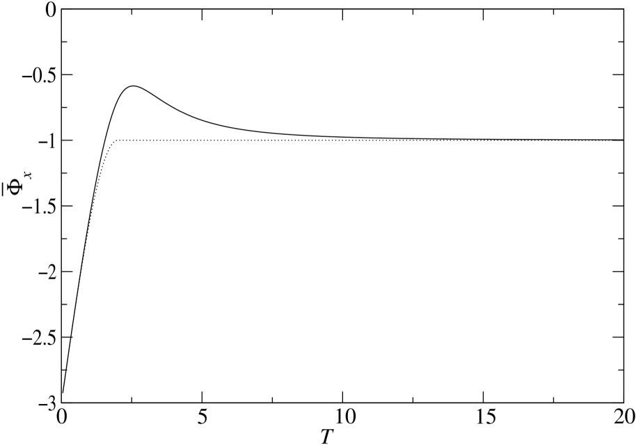
FIG. 1.: The normalized time-averaged self-force $\bar{\Phi}_{x}$ $\equiv$ $\bar{F}_{x}/\rho_{c}^{2}V^{2}D_{x}$ calculated using equation (34) for a trajectory $D_{x}(t_{1})$ = $D_{x}[1-\cos(2\pi t_{1}/T)]\Theta(T-t_{1})\Theta(t_{1})$ (solid curve), and using equations (1) and (30) for the steplike trajectory $D_{x}(t_{1})$ = $D_{x}\Theta(T-t_{1})\Theta(t_{1})$ (dotted curve). Units such that the speed of light $c=1$ and the radius of the body $R=1$ are used.

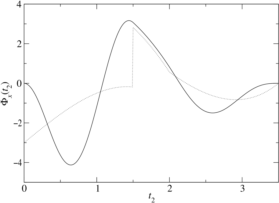
FIG. 2.: The normalized self-force $\Phi_{x}(t_{2})\equiv F_{x}(t_{2})/\rho_{c}^{2}V^{2}D_{x}$ calculated using equation (41) for a trajectory $D_{x}(t_{2})$ = $D_{x}[1-\cos(2\pi t_{2}/T)]\Theta(T-t_{2})\Theta(t_{2})$ (solid curve) and for the steplike trajectory $D_{x}(t_{2})$ = $D_{x}\Theta(T-t_{2})\Theta(t_{2})$ (dotted curve), with $T=1.5$. Units as in figure 1 are used.

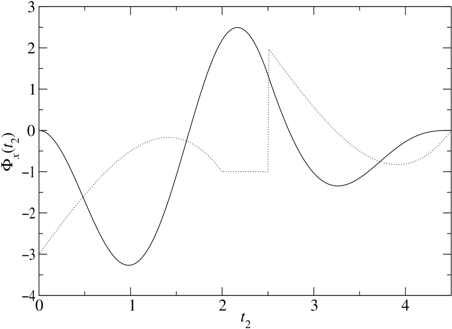
FIG. 3.: The normalized self-force $\Phi_{x}(t_{2})$ as in figure 2 but for a displacement duration $T=2.5$.

REFERENCES

• [1] Bohr N and Rosenfeld L 1933 Zur Frage der Messbarkeit der elektromagnetischen Feldgrössen Mat. Fys. Medd. K. Dan. Vidensk. Selsk. 12 no 8
Bohr N and Rosenfeld L 1983 On the question of the measurability of electromagnetic field quantities (Engl. transl.) Quantum Theory and Measurement ed J. A. Wheeler and W. H. Zurek (Princeton NJ: Princeton University Press) pp 479–522
• [2] Hnizdo V 1999 Geometric factors in the Bohr–Rosenfeld analysis of the measurability of the electromagnetic field J. Phys. A: Math. Gen. 32 2427–45
• [3] Compagno G and Persico F 1998 Limits on the measurability of the local quantum electromagnetic-field amplitude Phys. Rev. A 57 1595–1603
• [4] Hnizdo V 1999 Comment on Limits of the measurability of the local quantum electromagnetic-field amplitude Phys. Rev. A 60 4191–95
• [5] Compagno G and Persico F 1999 Reply to Comment on Limits of the measurability of the local quantum electromagnetic-field amplitude Phys. Rev. A 60 4196–97
• [6] Jackson J D 1975 Classical Electrodynamics 2nd edn (New York: Wiley) p 789, equation (17.28)
Refer to caption