A New Geometric Probability Technique for an N-dimensional Sphere and Its Applications to Physics

Abstract

A new formalism is presented for analytically obtaining the probability density function, $P_{n}(s)$, for the distance between two random points in an $n$-dimensional sphere of radius $R$. Our formalism allows $P_{n}(s)$ to be calculated for a sphere having an arbitrary density distribution, and reproduces the well-known results for the case of a sphere with uniform density. The results find applications in stochastic geometry, probability distribution theory, astrophysics, nuclear physics, and elementary particle physics.

I Introduction

In a recent paper [1], geometric probability techniques were developed to calculate the probability density functions (PDFs) which describe the probability density of finding a distance $s$ separating two points distributed in a uniform $3$-dimensional sphere and in a uniform ellipsoid. Our focus in the present paper will be on the probability density functions $P_{n}(s)$ for an $n$-dimensional sphere of radius $R$ characterized by $x_{1}^{2}+x_{2}^{2}+\cdots+x_{n}^{2}\leq R^{2}$, where $x_{1}$, $x_{2}$, and $x_{n}$ are the corresponding Cartesian coordinates. (In the mathematical literature this is sometimes termed an $n$-dimensional ball). As discussed in Refs. [1, 2, 3, 4], these results are of interest both as pure mathematics and as tools in mathematical physics. Specifically, it was demonstrated in Ref. [1] that geometric probability techniques greatly facilitate the calculation of the self-energies for spherical matter distributions arising from electromagnetic, gravitational, or weak interactions. The functional form of $P_{n}(s)$ is known for a sphere of uniform density, and hence the object of the present paper is to generalize the results of Refs. [2, 3, 4] to the case of an arbitrarily non-uniform density distribution by using our method. As an application of these results we will consider the neutrino-exchange contribution to the self-energy of a neutron star modeled as series of concentric shells of different constant density. Other applications will also be discussed.

In this paper we present a new technique for obtaining the analytical probability density function $P_{n}(s)$ for a sphere of $n$ dimensions having an arbitrary density distribution. To illustrate this technique, we begin by deriving the PDF, $P_{n}(s)$, for an $n$-dimensional uniform sphere of radius $R$, and compare our results to those obtained earlier by other means [2, 3, 4]. We then extend this technique to an $n$-dimensional sphere with a non-uniform but spherically symmetric density distribution. We explicitly evaluate the analytical probability density functions for certain specific density distributions, and then use numerical Monte Carlo simulations to verify the analytical results.

Finally our formalism is generalized to an $n$-dimensional sphere with an arbitrary density distribution, and leads to a general-purpose master formula. This formula allows one to evaluate the PDF for a sphere in $n$ dimensions with an arbitrary density distribution. After verifying that the master formula reproduces the results for uniform and spherically symmetric density distributions, we analytically evaluate the probability density functions, for 2, 3, and 4-dimensional spheres having non-uniform density distributions. The analytical results are then verified by the use of Monte Carlo simulations. The outline of this paper is as follows. In Sec. II we present our new formalism and illustrate it by rederiving the well-known results for a circle and for a sphere of uniform density. In Sec. III we extend this formalism to the case of non-uniform but spherically symmetric density distributions. In Sec. IV we develop the formalism for the most general case of an arbitrary non-uniform density distribution. In Sec. V we present some applications of our formalism to physics. These include the $m$th moment $\left\langle s^{m}\right\rangle$ for a sphere of uniform and Gaussian density distribution, Coulomb self-energy for a collection of charges, $\nu\bar{\nu}$-exchange interactions, obtaining the probability density functions for multiple-shell density distributions found in neutron star models [5, 6], and the evaluation of some geometric probability constants [7, 8].

II Uniform density distributions

A Theory for a uniform circle

In this section we illustrate our formalism by deriving the PDF for a circle of radius $R$ having a spatially uniform density distribution characterized by $\rho=$ constant. For two points randomly sampled inside the circle located at $\vec{r}_{1}$ and $\vec{r}_{2}$ measured from the center, define $\vec{s}=\vec{s}\left(\vec{r}_{1},\vec{r}_{2}\right)=\vec{r}_{2}-\vec{r}_{1}$ and $s=\left|\vec{s}\,\right|$. To simplify the discussion, we translate the center of the circle to the origin so that the equation for the circle is $x^{2}+y^{2}=R^{2}$. It is sufficient to initially consider those vectors $\vec{s}$ which are aligned in the positive $\hat{x}$ direction, since rotational symmetry can eventually be used to extend our results to those vectors $\vec{s}$ with arbitrary orientations. We begin by identifying those pairs of points, $\vec{r}_{1}$ and $\vec{r}_{2}$, which satisfy $\vec{s}=\vec{r}_{2}-\vec{r}_{1}=s\hat{x}$, where $0\leq s\leq 2R$. One set of points is obtained if the points 1 are uniformly located on a line $L_{1}$ given by $x=-s/2$ and the corresponding points 2 are on a line $L_{2}$ given by $x=+s/2$ as shown in Fig. 1. Notice that $x=\pm s/2$ are two symmetric lines with respect to reflection about $x=0$. Another set of points is obtained if $\vec{r}_{1}$ is uniformly located in the area $A_{1}$ and $\vec{r}_{2}$ is located in the area $A_{2}$ as shown in Fig. 2(a). Note that $A_{1}$ and $A_{2}$ are congruent. The only remaining set of points that need to be considered are those for which $\vec{r}_{1}$ is uniformly located in the area $A_{3}$ while $\vec{r}_{2}$ is in the area $A_{4}$ as shown in Fig. 2(b). As before $A_{3}$ and $A_{4}$ are congruent. Furthermore, $A_{4}$ is a reflection of $A_{2}$ about $x=s/2$, while $A_{3}$ is a reflection of $A_{1}$ about $x=-s/2$. As discussed in Appendix A, the union of $A_{2}$ and $A_{4}$ ($A_{2}\bigcup A_{4}$) is the overlap area between the original circle $C_{0}$ and an identical circle $C_{1}$ whose center is shifted from $\left(0,0\right)$ to $\left(\left|\vec{s}\,\right|,0\right)$. Similarly, $A_{1}\bigcup A_{3}$ is the overlap area between the original circle and an identical circle $C_{2}$ whose center is shifted from $\left(0,0\right)$ to $\left(-\left|\vec{s}\,\right|,0\right)$ as shown in Fig. 3. Since $A_{1}\bigcup A_{3}$ and $A_{2}\bigcup A_{4}$ are identical, it follows that the probability of finding a given $s=\left|s\hat{x}\right|$ in a uniform circle is proportional to

$$A_{2}\bigcup A_{4}=\int_{\frac{s}{2}}^{R}dx\int_{-\sqrt{R^{2}-x^{2}}}^{\sqrt{R^{2}-x^{2}}}dy+\int_{s-R}^{\frac{s}{2}}dx\int_{-\sqrt{R^{2}-(x-s)^{2}}}^{\sqrt{R^{2}-(x-s)^{2}}}dy.$$ (1)

Notice that

$\displaystyle\int_{\frac{s}{2}}^{R}dx\int_{-\sqrt{R^{2}-x^{2}}}^{\sqrt{R^{2}-x^{2}}}dy=\int_{s-R}^{\frac{s}{2}}dx\int_{-\sqrt{R^{2}-(x-s)^{2}}}^{\sqrt{R^{2}-(x-s)^{2}}}dy.$

Using rotational symmetry of $C_{0}$, this result can apply to any orientation of $\vec{s}$ between $0$ and $2\pi$, and hence the probability of finding a given $s=\left|\vec{s}\,\right|$ is proportional to $|\vec{s}\,|\int_{0}^{2\pi}d\phi=2\pi s$. We denote this PDF for a uniform circle by $P_{2}(s)$, and impose the normalization requirement

$$\int_{0}^{2R}P_{2}(s)ds=1.$$ (2)

We then have

$$P_{2}(s) = \frac{2\pi s\left(\int_{\frac{s}{2}}^{R}dx\int_{-\sqrt{R^{2}-x^{2}}}^{\sqrt{R^{2}-x^{2}}}dy+\int_{s-R}^{\frac{s}{2}}dx\int_{-\sqrt{R^{2}-(x-s)^{2}}}^{\sqrt{R^{2}-(x-s)^{2}}}dy\right)}{\int_{0}^{2R}2\pi s\left(\int_{\frac{s}{2}}^{R}dx\int_{-\sqrt{R^{2}-x^{2}}}^{\sqrt{R^{2}-x^{2}}}dy+\int_{s-R}^{\frac{s}{2}}dx\int_{-\sqrt{R^{2}-(x-s)^{2}}}^{\sqrt{R^{2}-(x-s)^{2}}}dy\right)ds}.$$ (3)

Equation (3) can be simplified to

$$P_{2}(s) = \frac{s\int_{\frac{s}{2}}^{R}dx\int_{-\sqrt{R^{2}-x^{2}}}^{\sqrt{R^{2}-x^{2}}}dy}{\int_{0}^{2R}\left(s\int_{\frac{s}{2}}^{R}dx\int_{-\sqrt{R^{2}-x^{2}}}^{\sqrt{R^{2}-x^{2}}}dy\right)ds}$$ (4)

$$= \frac{2s}{R^{2}}-\frac{s^{2}}{\pi R^{4}}\sqrt{4R^{2}-s^{2}}-\frac{4s}{\pi R^{2}}\sin^{-1}\left(\frac{s}{2R}\right).$$ (5)

Equation (5) is identical to the results obtained in Refs. [2, 3] by other means.

The conclusion that emerges from this formalism is that the probability of finding two random points separated by a vector $\vec{s}$ in a uniform circle can be derived by simply calculating the overlap region of that circle with an identical circle obtained by shifting the center from the origin to $\vec{s}$. In the following sections, we show that this result generalizes to higher dimensions, and provides a simple way of calculating $P_{n}(s)$ for $n\geq 3$.

B Theory for a uniform sphere

The above formalism for a $2$-dimensional uniform circle can be extended to a $3$-dimensional uniform sphere with radius $R$. For a given $s$, we arbitrarily select the positive $\hat{z}$ direction and study the distribution of vectors $\vec{s}=\vec{r}_{2}-\vec{r}_{1}$ in this direction. The areas $A_{1}$, $A_{2}$, $A_{3}$, and $A_{4}$ in Sec. II A are replaced by the volumes $V_{1}$, $V_{2}$, $V_{3}$, and $V_{4}$. The PDF $P_{3}(s)$ is therefore proportional to the overlap volume $V_{1}\bigcup V_{3}=V_{2}\bigcup V_{4}$, where

$$V_{2}\bigcup V_{4}=\int_{\frac{s}{2}}^{R}dz\int_{-\sqrt{R^{2}-z^{2}}}^{\sqrt{R^{2}-z^{2}}}dx\int^{\sqrt{R^{2}-z^{2}-x^{2}}}_{-\sqrt{R^{2}-z^{2}-x^{2}}}dy+\int_{s-R}^{\frac{s}{2}}dz\int_{-\sqrt{R^{2}-(z-s)^{2}}}^{\sqrt{R^{2}-(z-s)^{2}}}dx\int^{\sqrt{R^{2}-(z-s)^{2}-x^{2}}}_{-\sqrt{R^{2}-(z-s)^{2}-x^{2}}}dy.$$ (6)

Notice that

$$\int_{\frac{s}{2}}^{R}dz\int_{-\sqrt{R^{2}-z^{2}}}^{\sqrt{R^{2}-z^{2}}}dx\int^{\sqrt{R^{2}-z^{2}-x^{2}}}_{-\sqrt{R^{2}-z^{2}-x^{2}}}dy=\int_{s-R}^{\frac{s}{2}}dz\int_{-\sqrt{R^{2}-(z-s)^{2}}}^{\sqrt{R^{2}-(z-s)^{2}}}dx\int^{\sqrt{R^{2}-(z-s)^{2}-x^{2}}}_{-\sqrt{R^{2}-(z-s)^{2}-x^{2}}}dy.$$ (7)

In a $3$-dimensional space, $\vec{s}$ can range from $0$ to $\pi$ in the $\hat{\theta}$ direction, and from $0$ to $2\pi$ in the $\hat{\phi}$ direction. For a given $s$ with any orientation, the PDF $P_{3}(s)$ is also proportional to $4\pi s^{2}$ by using rotational symmetry of a uniform sphere. Following the previous discussion, we thus arrive at the following expression for the PDF for a uniform sphere:

$$P_{3}(s) = \frac{4\pi s^{2}\left(\int_{\frac{s}{2}}^{R}dz\int_{-\sqrt{R^{2}-z^{2}}}^{\sqrt{R^{2}-z^{2}}}dx\int^{\sqrt{R^{2}-z^{2}-x^{2}}}_{-\sqrt{R^{2}-z^{2}-x^{2}}}dy\right)}{\int_{0}^{2R}4\pi s^{2}\left(\int_{\frac{s}{2}}^{R}dz\int_{-\sqrt{R^{2}-z^{2}}}^{\sqrt{R^{2}-z^{2}}}dx\int^{\sqrt{R^{2}-z^{2}-x^{2}}}_{-\sqrt{R^{2}-z^{2}-x^{2}}}dy\right)ds}$$ (8)

$$= 3\frac{s^{2}}{R^{3}}-\frac{9}{4}\frac{s^{3}}{R^{4}}+\frac{3}{16}\frac{s^{5}}{R^{6}}.$$ (9)

The result in Eq. (9) agrees exactly with the expression obtained previously in Refs. [2, 3, 4].

C Representations , general properties, recursion relations, and generating functions of $P_{n}(s)$

The present formalism can be readily generalized to obtain $P_{n}(s)$ for an $n$-dimensional sphere ($n$-sphere or $n$-ball) of radius $R$. From Eqs. (4) and (8) we find

$$P_{n}(s)=\frac{s^{n-1}\int_{\frac{s}{2}}^{R}dx_{n}\int_{-\sqrt{R^{2}-x_{n}^{2}}}^{\sqrt{R^{2}-x_{n}^{2}}}dx_{1}\int_{-\sqrt{R^{2}-x_{n}^{2}-x_{1}^{2}}}^{\sqrt{R^{2}-x_{n}^{2}-x_{1}^{2}}}dx_{2}\cdots\int_{-\sqrt{R^{2}-x_{n}^{2}-\cdots x_{n-2}^{2}}}^{\sqrt{R^{2}-x_{n}^{2}-\cdots x_{n-2}^{2}}}dx_{n-1}}{\int_{0}^{2R}\left(s^{n-1}\int_{\frac{s}{2}}^{R}dx_{n}\int_{-\sqrt{R^{2}-x_{n}^{2}}}^{\sqrt{R^{2}-x_{n}^{2}}}dx_{1}\int_{-\sqrt{R^{2}-x_{n}^{2}-x_{1}^{2}}}^{\sqrt{R^{2}-x_{n}^{2}-x_{1}^{2}}}dx_{2}\cdots\int_{-\sqrt{R^{2}-x_{n}^{2}-\cdots x_{n-2}^{2}}}^{\sqrt{R^{2}-x_{n}^{2}-\cdots x_{n-2}^{2}}}dx_{n-1}\right)ds}.$$ (10)

We can rewrite Eq. (10) as

$$P_{n}(s)=\frac{s^{n-1}\int_{\frac{s}{2}}^{R}dx_{n}\int_{-\overline{R}}^{\overline{R}}dx_{1}\int^{\sqrt{\overline{R}^{2}-x_{1}^{2}}}_{-\sqrt{\overline{R}^{2}-x_{1}^{2}}}dx_{2}\cdots\int_{-\sqrt{\overline{R}^{2}-x_{1}^{2}-\cdots x_{n-2}^{2}}}^{\sqrt{\overline{R}^{2}-x_{1}^{2}-\cdots x_{n-2}^{2}}}dx_{n-1}}{\int_{0}^{2R}\left(s^{n-1}\int_{\frac{s}{2}}^{R}dx_{n}\int_{-\overline{R}}^{\overline{R}}dx_{1}\int^{\sqrt{\overline{R}^{2}-x_{1}^{2}}}_{-\sqrt{\overline{R}^{2}-x_{1}^{2}}}dx_{2}\cdots\int_{-\sqrt{\overline{R}^{2}-x_{1}^{2}-\cdots x_{n-2}^{2}}}^{\sqrt{\overline{R}^{2}-x_{1}^{2}-\cdots x_{n-2}^{2}}}dx_{n-1}\right)ds},$$ (11)

where

$$\overline{R}=\sqrt{R^{2}-x_{n}^{2}}.$$ (12)

As shown in Refs. [9, 10, 11], the volume $V(n,R)$ of an $n$-dimensional sphere of radius $R$ is given by

$$V\left(n,R\right)=\int_{-R}^{R}dx_{1}\int^{\sqrt{R^{2}-x_{1}^{2}}}_{-\sqrt{R^{2}-x_{1}^{2}}}dx_{2}\cdots\int_{-\sqrt{R^{2}-x_{1}^{2}-x_{2}^{2}-\cdots x_{n-1}^{2}}}^{\sqrt{R^{2}-x_{1}^{2}-x_{2}^{2}-\cdots x_{n-1}^{2}}}dx_{n}=\frac{\pi^{\frac{n}{2}}R^{n}}{\Gamma\left(1+\frac{n}{2}\right)}.$$ (13)

Equations. (10) and (11) can then be reduced to a general simplified equation for an $n$-dimensional uniform sphere of radius $R$:

$$P_{n}(s) = \frac{s^{n-1}\int_{\frac{s}{2}}^{R}\frac{\pi^{\frac{n-1}{2}}}{\Gamma\left(1+\frac{n-1}{2}\right)}\left(\sqrt{R^{2}-x_{n}^{2}}\right)^{\left(n-1\right)}dx_{n}}{\int_{0}^{2R}\left[s^{n-1}\int_{\frac{s}{2}}^{R}\frac{\pi^{\frac{n-1}{2}}}{\Gamma\left(1+\frac{n-1}{2}\right)}\left(\sqrt{R^{2}-x_{n}^{2}}\right)^{\left(n-1\right)}dx_{n}\right]ds}$$ (14)

$$= \frac{s^{n-1}\int_{\frac{s}{2}}^{R}\left(R^{2}-x^{2}\right)^{\frac{n-1}{2}}dx}{\int_{0}^{2R}\left[s^{n-1}\int_{\frac{s}{2}}^{R}\left(R^{2}-x^{2}\right)^{\frac{n-1}{2}}dx\right]ds}.$$ (15)

If $n$ is an even number,

$$P_{n}(s)=n\times\frac{s^{n-1}}{R^{n}}\left[\frac{2}{\pi}\cos^{-1}\left(\frac{s}{2R}\right)-\frac{s}{\pi}\sum_{k=1}^{\frac{n}{2}}\frac{(n-2k)!!}{(n-2k+1)!!}\left(R^{2}-\frac{s^{2}}{4}\right)^{\frac{n-2k+1}{2}}R^{2k-2-n}\right],$$ (16)

where $0!=0!!=1$. If $n$ is an odd number,

$$P_{n}(s)=n\times\frac{s^{n-1}}{R^{n}}\frac{n!!}{(n-1)!!}\sum_{k=0}^{\frac{n-1}{2}}\frac{(-1)^{k}}{2k+1}\frac{\left(\frac{n-1}{2}\right)!}{k!\left(\frac{n-1}{2}-k\right)!}\left[1-\left(\frac{s}{2R}\right)^{2k+1}\right].$$ (17)

Using Eqs. (16) and (17) the explicit functional forms of $P_{n}(s)$ for $n=2$, $3$, $4$, and $5$ are as follows:

$$P_{2}(s) = \frac{4}{\pi}\frac{s}{R^{2}}\cos^{-1}\left(\frac{s}{2R}\right)-\frac{2}{\pi}\frac{s^{2}}{R^{3}}\left(1-\frac{s^{2}}{4R^{2}}\right)^{1/2},$$ (18)

$$P_{4}(s) = \frac{8}{\pi}\frac{s^{3}}{R^{4}}\cos^{-1}\left(\frac{s}{2R}\right)-\frac{8}{3\pi}\frac{s^{4}}{R^{5}}\left(1-\frac{s^{2}}{4R^{2}}\right)^{3/2}-\frac{4}{\pi}\frac{s^{4}}{R^{5}}\left(1-\frac{s^{2}}{4R^{2}}\right)^{1/2},$$ (19)

$$P_{3}(s) = 3\frac{s^{2}}{R^{3}}-\frac{9}{4}\frac{s^{3}}{R^{4}}+\frac{3}{16}\frac{s^{5}}{R^{6}},$$ (20)

$$P_{5}(s) = 5\frac{s^{4}}{R^{5}}-\frac{75}{16}\frac{s^{5}}{R^{6}}+\frac{25}{32}\frac{s^{7}}{R^{8}}-\frac{15}{256}\frac{s^{9}}{R^{10}}.$$ (21)

The Monte Carlo results for $n\geq 4$, and the simulation techniques for producing random points uniformly inside an $n$-sphere will be presented elsewhere [7, 8].

It is of interest to verify that Eq. (15), obtained via the present formalism, agrees with results obtained earlier by other means [2, 3]. This is most easily done by introducing the the function $C(a;\,m,n)$ defined by

$$C(a;\,m,n)=\int_{0}^{a}s^{m}T_{n}(s)ds=\int_{0}^{a}s^{m+n-1}Q_{n}(s)ds=\int_{0}^{a}s^{m+n-1}\,ds\int_{\frac{s}{2}}^{R}\left(R^{2}-x^{2}\right)^{\frac{n-1}{2}}\,dx,$$ (22)

where

$$Q_{n}(s) = \int_{\frac{s}{2}}^{R}\left(R^{2}-x^{2}\right)^{\frac{n-1}{2}}dx,$$ (23)

$$T_{n}(s) = s^{n-1}\int_{\frac{s}{2}}^{R}\left(R^{2}-x^{2}\right)^{\frac{n-1}{2}}dx.$$ (24)

It follows that the denominator of Eq. (15), which is the normalization constant, can be written as $C(2R;\,0,n)$ where

$$C(2R;\,0,n) = \int_{0}^{2R}T_{n}(s)ds.$$ (25)

When $n$ is an even integer, $C(2R;\,0,n)$ can be expressed in terms of the gamma and beta functions by noting that

$$C(2R;\,0,n)=\frac{\pi}{2n}\frac{(n-1)!!}{n!!}R^{2n}=\frac{1}{2n}\frac{\Gamma\left(\frac{1}{2}\right)\Gamma\left(\frac{n}{2}+\frac{1}{2}\right)}{\Gamma\left(\frac{n}{2}+1\right)}R^{2n}=\frac{1}{2n}B\left(\frac{n}{2}+\frac{1}{2},\frac{1}{2}\right)R^{2n}.$$ (26)

Similarly, when $n$ is an odd integer,

$$C(2R;\,0,n)=\frac{1}{n}\frac{(n-1)!!}{n!!}R^{2n}=\frac{1}{2n}B\left(\frac{n}{2}+\frac{1}{2},\frac{1}{2}\right)R^{2n}.$$ (27)

We thus find that the normalization constant has the same functional form irrespective of whether $n$ is even or odd, when expressed in terms of the beta function.

If we introduce the variable $t=R^{2}-x^{2}$ and note that

$$Q_{n}(s)=\frac{R^{n}}{2}B_{1-\frac{s^{2}}{4R^{2}}}\left(\frac{n}{2}+\frac{1}{2},\frac{1}{2}\right)=\frac{R^{n}}{2}B\left(\frac{n}{2}+\frac{1}{2},\frac{1}{2}\right)I_{1-\frac{s^{2}}{4R^{2}}}\left(\frac{n}{2}+\frac{1}{2},\frac{1}{2}\right),$$ (28)

we can then rewrite $P_{n}(s)$ in the form

$$P_{n}(s) = n\frac{s^{n-1}}{R^{n}}\frac{B_{x}\left(\frac{n}{2}+\frac{1}{2},\frac{1}{2}\right)}{B\left(\frac{n}{2}+\frac{1}{2},\frac{1}{2}\right)}$$ (29)

$$= n\frac{s^{n-1}}{R^{n}}I_{x}\left(\frac{n}{2}+\frac{1}{2},\frac{1}{2}\right),$$ (30)

where

$$x=1-\frac{s^{2}}{4R^{2}}.$$ (31)

$B_{x}\left(p,q\right)$ is the incomplete beta function defined by

$$B_{x}\left(p,q\right)=\int_{0}^{x}t^{p-1}\left(1-t\right)^{q-1}dt,$$ (32)

and $I_{x}$ is the normalized incomplete beta function defined by

$$I_{x}(p,q)=\frac{\Gamma\left(p+q\right)}{\Gamma\left(p\right)\Gamma\left(q\right)}\int_{0}^{x}t^{p-1}\left(1-t\right)^{q-1}dt=\frac{B_{x}(p,q)}{B(p,q)}.$$ (33)

Eq. (30) is the expression for $P_{n}(s)$ obtained in Refs. [2, 3], and hence we have demonstrated that the classical results can be reproduced by using the formalism developed here.

We find the following general properties of $P_{n}(s)$ and its derivative $P^{\prime}_{n}(s)$ at the lower bound $s=0$ and at the upper bound $s=2R$: $P_{1}(0)=1/R$, $P_{n}(0)=0$ for $n\geq 2$, $P_{n}(2R)=0$, $P_{1}^{\prime}(0)=-1/2R^{2}$, $P_{2}^{\prime}(0)=2/R^{2}$, $P_{n}^{\prime}(0)=0$ for $n\geq 3$, $P_{1}^{\prime}(2R)=-1/2R^{2}$, and $P_{n}^{\prime}(2R)=0$ for $n\geq 2$.

It is of interest to express the probability density functions $P_{n}(s)$ in terms of generating functions from which several representations and recursion relations for $P_{n}(s)$ can be derived. This can be achieved by observing that

$$B_{x}\left(\frac{n}{2}+\frac{1}{2},\frac{1}{2}\right)=\frac{1}{n!}\left(\frac{\partial}{\partial h}\right)^{n}F(h=0,x),$$ (34)

where

$$F(h,x)=\frac{2}{\sqrt{1-h^{2}}}\left[\sin^{-1}(h)\,-\sin^{-1}\left(\frac{h-\sqrt{x}}{1-h\sqrt{x}}\right)\right],$$ (35)

and where $0\leq x\leq 1$ and $-1\leq h\leq 1$. Similarly, $Q_{n}(s)$ in Eq. (23) can be defined in terms of a generating function $F_{1}(h,s)$ of the form

$$F_{1}(h,s)=\sum_{n=0}^{\infty}Q_{n}(s)h^{n}=\frac{1}{\sqrt{1-h^{2}R^{2}}}\left[\sin^{-1}(hR)-\sin^{-1}\left(\frac{hR-\sqrt{1-\frac{s^{2}}{4R^{2}}}}{1-hR\sqrt{1-\frac{s^{2}}{4R^{2}}}}\right)\right],$$ (36)

where $\left|hR\right|<1$. $Q_{n}(s)$ is then given by

$$Q_{n}(s)=\frac{1}{n!}\left(\frac{\partial}{\partial h}\right)^{n}F_{1}(h=0,s).$$ (37)

$T_{n}(s)$ in Eq. (24) can also be defined in terms of a generating function $F_{2}(h,s)$,

$$F_{2}(h,s)=\sum_{n=0}^{\infty}T_{n}(s)h^{n}=\left(\frac{1}{s}\right)\frac{1}{\sqrt{1-h^{2}R^{2}s^{2}}}\left[\sin^{-1}(hRs)-\sin^{-1}\left(\frac{hRs-\sqrt{1-\frac{s^{2}}{4R^{2}}}}{1-hRs\sqrt{1-\frac{s^{2}}{4R^{2}}}}\right)\right],$$ (38)

where $\left|hRs\right|<1$. $T_{n}(s)$ is then given by

$$T_{n}(s)=\frac{1}{n!}\left(\frac{\partial}{\partial h}\right)^{n}F_{2}(h=0,s).$$ (39)

It follows from the previous results that $P_{n}(s)$ can be expressed in terms of two unique elementary functions, $F_{1}(h,s)$ in Eq. (36) and $F_{2}(h,s)$ in Eq. (38), such that

$$P_{n}(s)=\frac{\frac{1}{n!}\left(\frac{\partial}{\partial h}\right)^{n}F_{2}(h=0,s)}{\frac{1}{2n}B(\frac{n}{2}+\frac{1}{2},\frac{1}{2})R^{2n}}=\frac{s^{n-1}\frac{1}{n!}\left(\frac{\partial}{\partial h}\right)^{n}F_{1}(h=0,s)}{\frac{1}{2n}B(\frac{n}{2}+\frac{1}{2},\frac{1}{2})R^{2n}}.$$ (40)

It is convenient to summarize the different expressions we have obtained for the PDF of a uniform $n$-dimensional sphere with radius $R$:

1. Integral representation:

   $$P_{n}(s)=\frac{s^{n-1}\int_{\frac{s}{2}}^{R}\left(R^{2}-x^{2}\right)^{\frac{n-1}{2}}dx}{\frac{1}{2n}B(\frac{n}{2}+\frac{1}{2},\frac{1}{2})R^{2n}},$$ (41)

2. Normalized incomplete beta function representation:

   $$P_{n}(s)=n\frac{s^{n-1}}{R^{n}}I_{1-\frac{s^{2}}{4R^{2}}}\left(\frac{n}{2}+\frac{1}{2},\frac{1}{2}\right),$$ (42)

3. Incomplete beta function representation:

   $$P_{n}(s)=n\frac{s^{n-1}B_{1-\frac{s^{2}}{4R^{2}}}\left(\frac{n}{2}+\frac{1}{2},\frac{1}{2}\right)}{B\left(\frac{n}{2}+\frac{1}{2},\frac{1}{2}\right)R^{n}},$$ (43)

4. Odd-integer finite series expansion representation ($n=$ odd):

   $$P_{n}(s)=n\times\frac{s^{n-1}}{R^{n}}\frac{n!!}{(n-1)!!}\sum_{i=0}^{\frac{n-1}{2}}\frac{(-1)^{i}}{2i+1}\frac{\left(\frac{n-1}{2}\right)!}{i!\left(\frac{n-1}{2}-i\right)!}\left[1-\left(\frac{s}{2R}\right)^{2i+1}\right],$$ (44)

5. Even-integer finite series expansion representation ($n=$ even):

   $$P_{n}(s)=n\times\frac{s^{n-1}}{R^{n}}\left[\frac{2}{\pi}\cos^{-1}\left(\frac{s}{2R}\right)-\frac{s}{\pi}\sum_{i=1}^{\frac{n}{2}}\frac{(n-2i)!!}{(n-2i+1)!!}\left(R^{2}-\frac{s^{2}}{4}\right)^{\frac{n-2i+1}{2}}R^{2i-2-n}\right],$$ (45)

6. Infinite series expansion representation:

   $$P_{n}(s)=\frac{s^{n-1}\sum_{i=0}^{\infty}\left(-1\right)^{i}\frac{2^{i}}{2i+1}\frac{\left(2i-1\right)!!}{\left(2i\right)!!}\frac{\left(\frac{n-1}{2}\right)!}{\left(\frac{n-1}{2}-i\right)!}\left[1-\left(\frac{s}{2R}\right)^{2i+1}\right]}{\frac{1}{2n}B\left(\frac{n}{2}+\frac{1}{2},\frac{1}{2}\right)R^{n}},$$ (46)

7. Generating function representation I:

   $$P_{n}(s) = \frac{\frac{1}{n!}\left(\frac{\partial}{\partial h}\right)^{n}_{h=0}\left\{\left(\frac{1}{s}\right)\frac{1}{\sqrt{1-h^{2}R^{2}s^{2}}}\left[\sin^{-1}(hRs)-\sin^{-1}\left(\frac{hRs-\sqrt{1-\frac{s^{2}}{4R^{2}}}}{1-hRs\sqrt{1-\frac{s^{2}}{4R^{2}}}}\right)\right]\right\}}{\frac{1}{2n}B(\frac{n}{2}+\frac{1}{2},\frac{1}{2})R^{2n}},$$ (47)

8. Generating function representation II:

   $$P_{n}(s)=\frac{s^{n-1}\frac{1}{n!}\left(\frac{\partial}{\partial h}\right)^{n}_{h=0}\left\{\frac{1}{\sqrt{1-h^{2}R^{2}}}\left[\sin^{-1}(hR)-\sin^{-1}\left(\frac{hR-\sqrt{1-\frac{s^{2}}{4R^{2}}}}{1-hR\sqrt{1-\frac{s^{2}}{4R^{2}}}}\right)\right]\right\}}{\frac{1}{2n}B(\frac{n}{2}+\frac{1}{2},\frac{1}{2})R^{2n}},$$ (48)

9. Hypergeometric function representation:

   $$P_{n}(s)=\frac{2n}{B\left(\frac{n}{2}+\frac{1}{2},\frac{1}{2}\right)}\frac{s^{n-1}}{R^{n+1}}\left[R\,\,_{2}F_{1}\left(\frac{1}{2},\frac{1}{2}-\frac{n}{2};\frac{3}{2};1\right)-\frac{s}{2}\,\,_{2}F_{1}\left(\frac{1}{2},\frac{1}{2}-\frac{n}{2};\frac{3}{2};\frac{s^{2}}{4R^{2}}\right)\right],$$ (49)

   where

   $$\int\left(R^{2}-x^{2}\right)^{\frac{n-1}{2}}dx=R^{n-1}x\,\,_{2}F_{1}\left(\frac{1}{2},\frac{1}{2}-\frac{n}{2};\frac{3}{2};\frac{x^{2}}{R^{2}}\right),$$ (50)

   and

   $$y(x) \equiv \,\,{}_{2}F_{1}(a,b;c;x)$$ (51)

   $$= 1+\frac{ab}{c}\frac{x}{1!}+\frac{a(a+1)b(b+1)}{c(c+1)}\frac{x^{2}}{2!}+\frac{a(a+1)(a+2)b(b+1)(b+2)}{c(c+1)(c+2)}\frac{x^{3}}{3!}+\cdots,$$ (52)

   is one of the solutions for the hypergeometric equation

   $$x(1-x)y^{\prime\prime}(x)+\left[c-(a+b+1)x\right]y^{\prime}(x)-aby(x)=0.$$ (53)

Using the previous results one can obtain a number of identities and recursion relations for the probability density functions $P_{n}(s)$, as we discuss in Appendix B.

III Spherically symmetric density distributions

In this section we generalize the previous results to the case of an $n$-dimensional sphere of radius $R$ with a variable (but spherically symmetric) density distribution of the form $\rho=\rho(r)$, where $r=\sqrt{x_{1}^{2}+x_{2}^{2}+\cdots x_{n}^{2}}$ is measured from the center and

$\displaystyle x_{1}^{2}+x_{2}^{2}+\cdots+x_{n}^{2}\leq R^{2}.$

As before we begin with the example of a circle ($n=2$) and generalize to a sphere ($n\geq 3$) later. Following the derivation presented in the previous section, the positive $\hat{x}$ direction is chosen to specify the distribution of those $\vec{s}$ vectors that are aligned along the positive $\hat{x}$ direction. At this stage we must consider the differences between uniform and non-uniform density distributions. For a given $s,$ if point $2$ carries the density information $\rho(x,y)$, then point $1$ should have the density information $\rho(x-s,y).$ It follows that to incorporate the effects of a spherically symmetric density distribution the following substitution should be made:

$$\rho(\vec{r}_{2})\times\rho(\vec{r}_{1})\rightarrow\rho(x,y)\times\rho(x-s,y).$$ (54)

Since the density distributions considered are spherically symmetric, the probability of finding a given $s$ in any orientation is still proportional to $2\pi s.$ The PDF $P_{2}(s)$ can then be expressed in the form

$$P_{2}(s)=\frac{n_{d}(s)\times\left(n_{1}(s)+n_{2}(s)\right)}{\int_{0}^{2R}n_{d}(s)\times\left(n_{1}(s)+n_{2}(s)\right)ds},$$ (55)

where

$$n_{d}(s) = 2\pi s,$$ (56)

$$n_{1}(s) = \int_{s-R}^{\frac{s}{2}}dx\int_{-\sqrt{R^{2}-(x-s)^{2}}}^{\sqrt{R^{2}-(x-s)^{2}}}\rho(x,y)\times\rho(x-s,y)dy,$$ (57)

$$n_{2}(s) = \int_{\frac{s}{2}}^{R}dx\int_{-\sqrt{R^{2}-x^{2}}}^{\sqrt{R^{2}-x^{2}}}\rho(x,y)\times\rho(x-s,y)dy.$$ (58)

Substituting $x-s=x^{\prime}$ and using $\rho(x,y)=\rho(-x,y)$ it can be shown that $n_{1}(s)=n_{2}(s).$ The expression for $P_{2}(s)$ can then be simplified to read

$$P_{2}(s) = \frac{s\int_{\frac{s}{2}}^{R}dx\int_{-\sqrt{R^{2}-x^{2}}}^{\sqrt{R^{2}-x^{2}}}\rho(x,y)\times\rho(x-s,y)dy}{\int_{0}^{2R}\left(s\int_{\frac{s}{2}}^{R}dx\int_{-\sqrt{R^{2}-x^{2}}}^{\sqrt{R^{2}-x^{2}}}\rho(x,y)\times\rho(x-s,y)dy\right)ds}.$$ (59)

The formalism leading to Eq. (59) can be extended to a $3$-dimensional sphere of radius $R$. For a given $s$, the $z$-axis is chosen arbitrarily as our reference axis to examine the distribution of those $\vec{s}$ vectors that are aligned along the positive $\hat{z}$ direction. If the density at point $2$ is $\rho(x,y,z),$ then the density at point $1$ will be $\rho(x,y,z-s).$ In analogy with the $2$-dimensional case discussed above, the expression in Eq. (54) must be replaced by

$$\rho(\vec{r}_{2})\times\rho(\vec{r}_{1})=\rho(x,y,z)\times\rho(x,y,z-s).$$ (60)

Since the density distributions considered here are spherically symmetric, the probability of finding a given $s$ in any orientation is proportional to $4\pi s^{2}$. Hence $P_{3}(s)$ can be expressed as

$$P_{3}(s) = \frac{s^{2}\int_{\frac{s}{2}}^{R}dz\int_{-\sqrt{R^{2}-z^{2}}}^{\sqrt{R^{2}-z^{2}}}dx\int_{-\sqrt{R^{2}-z^{2}-x^{2}}}^{\sqrt{R^{2}-z^{2}-x^{2}}}\rho(x,y,z)\times\rho(x,y,z-s)dy}{\int_{0}^{2R}\left(s^{2}\int_{\frac{s}{2}}^{R}dz\int_{-\sqrt{R^{2}-z^{2}}}^{\sqrt{R^{2}-z^{2}}}dx\int_{-\sqrt{R^{2}-z^{2}-x^{2}}}^{\sqrt{R^{2}-z^{2}-x^{2}}}\rho(x,y,z)\times\rho(x,y,z-s)dy\right)ds}$$ (61)

$$= \frac{s^{2}\int^{R}_{\frac{s}{2}}dx_{3}\int_{-\sqrt{R^{2}-x_{3}^{2}}}^{\sqrt{R^{2}-x_{3}^{2}}}dx_{1}\int_{-\sqrt{R^{2}-x_{3}^{2}-x_{1}^{2}}}^{\sqrt{R^{2}-x_{3}^{2}-x_{1}^{2}}}dx_{2}\rho\left(x_{1},x_{2},x_{3}\right)\rho\left(x_{1},x_{2},x_{3}^{\prime}\right)}{\int_{0}^{2R}s^{2}ds\int^{R}_{\frac{s}{2}}dx_{3}\int_{-\sqrt{R^{2}-x_{3}^{2}}}^{\sqrt{R^{2}-x_{3}^{2}}}dx_{1}\int_{-\sqrt{R^{2}-x_{3}^{2}-x_{1}^{2}}}^{\sqrt{R^{2}-x_{3}^{2}-x_{1}^{2}}}dx_{2}\rho\left(x_{1},x_{2},x_{3}\right)\rho\left(x_{1},x_{2},x_{3}^{\prime}\right)},$$ (62)

where $x_{3}^{\prime}=x_{3}-s$.

Up to this point our discussion has been completely general. To continue we next evaluate $P_{3}(s)$ for a $3$-dimensional sphere of radius $R$ using two different spherically symmetric density distributions. Consider first

$$\rho(r)=\frac{5N}{4\pi R^{5}}r^{2},$$ (63)

where $N=4\pi\int_{0}^{R}r^{2}\rho(r)dr$, and $r$ is measured from the center of the spherical distribution. Combining Eqs. (62) and (63) we find

$$P_{3}(s)=\frac{25}{7}\frac{s^{2}}{R^{3}}-\frac{25}{4}\frac{s^{3}}{R^{4}}+5\frac{s^{4}}{R^{5}}-\frac{25}{16}\frac{s^{5}}{R^{6}}+\frac{5}{448}\frac{s^{9}}{R^{10}}.$$ (64)

A plot of Eq. (64) when $R=1$, along with the corresponding Monte Carlo results, is shown in Fig. 4. The second spherically symmetric distribution we consider is

$$\rho(r)=\frac{N}{4\pi\left(\frac{1}{3}-\frac{\alpha}{5}\right)R^{3}}\left[1-\alpha\left(\frac{r}{R}\right)^{2}\right],$$ (65)

where $N=4\pi\int_{0}^{R}r^{2}\rho(r)dr$, $0\leq\alpha\leq 1$, and $r$ is measured from the center. Combining Eqs. (62) and (65) we find

$$P_{3}(s) = \frac{15(35-42\alpha+15\alpha^{2})s^{2}}{7(5-3\alpha)^{2}R^{3}}-\frac{225(1-\alpha)^{2}s^{3}}{4(5-3\alpha)^{2}R^{4}}-\frac{15\alpha s^{4}}{(5-3\alpha)R^{5}}$$ (67)

$$+\frac{75(1+6\alpha-3\alpha^{2})s^{5}}{16(5-3\alpha)^{2}R^{6}}-\frac{15\alpha s^{7}}{8(5-3\alpha)^{2}R^{8}}+\frac{45\alpha^{2}s^{9}}{448(5-3\alpha)^{2}R^{10}}.$$

A plot of Eq. (67) when $R=\alpha=1$ is shown in Fig. 5, along with the corresponding Monte Carlo results.

A general formula for the probability density function for an $n$-dimensional sphere with radius $R$ having a spherically symmetric density distribution can be derived from the previous results. We find

$$P_{n}(s)=\frac{s^{n-1}\int_{\frac{s}{2}}^{R}dx_{n}\int_{-\sqrt{R^{2}-x_{n}^{2}}}^{\sqrt{R^{2}-x_{n}^{2}}}dx_{1}\cdots\cdots\int_{-\sqrt{R^{2}-x_{n}^{2}-x_{1}^{2}-\cdots x_{n-1}^{2}}}^{\sqrt{R^{2}-x_{n}^{2}-x_{1}^{2}-\cdots x_{n-1}^{2}}}\rho\left(\mathbf{X}\right)\rho\left(\mathbf{X}^{\prime}\right)dx_{n-1}}{\int_{0}^{2R}\left[s^{n-1}\int_{\frac{s}{2}}^{R}dx_{n}\int_{-\sqrt{R^{2}-x_{n}^{2}}}^{\sqrt{R^{2}-x_{n}^{2}}}dx_{1}\cdots\cdots\int_{-\sqrt{R^{2}-x_{n}^{2}-x_{1}^{2}-\cdots x_{n-1}^{2}}}^{\sqrt{R^{2}-x_{n}^{2}-x_{1}^{2}-\cdots x_{n-1}^{2}}}\rho\left(\mathbf{X}\right)\rho\left(\mathbf{X}^{\prime}\right)dx_{n-1}\right]ds},$$ (68)

where

$$\rho(\mathbf{X}) = \rho(x_{1},x_{2},x_{3},\cdots\cdots,x_{n}),$$ (69)

$$\rho(\mathbf{X}^{\prime}) = \rho(x_{1},x_{2},x_{3},\cdots\cdots,x_{n}-s).$$ (70)

Another density distribution we wish to study is a Gaussian. As an example, consider the case of an $n$-dimensional sphere of radius $R\rightarrow\infty$ with a Gaussian density distribution $\rho(r)$ given by

$$\rho_{n}(r)=\frac{N}{(2\pi)^{\frac{n}{2}}\sigma^{n}}e^{-\frac{1}{2}\frac{r^{2}}{\sigma^{2}}},$$ (71)

where

$$N=\lim_{R\rightarrow\infty}n\frac{\pi^{\frac{n}{2}}}{\Gamma\left(\frac{n}{2}+1\right)}\int_{0}^{R}\rho_{n}(r)r^{n-1}dr.$$ (72)

In Eq. (72) $r$ is measured from the center of the spherical distribution and the integral is over all space. Recall that

$$\int_{0}^{\infty}x^{n}e^{-\frac{x^{2}}{2\sigma^{2}}}dx = 2^{\frac{n-1}{2}}\Gamma\left(\frac{n+1}{2}\right)\sigma^{n+1}.$$ (73)

Combining Eqs. (71) and (73), the PDF for an $n$-dimensional sphere in an infinite space with a Gaussian density distribution can be expressed as

$$P_{n}(s)=\lim_{R\rightarrow\infty}\frac{s^{n-1}e^{-\frac{s^{2}}{4\sigma^{2}}}}{\int_{0}^{2R}s^{n-1}e^{-\frac{s^{2}}{4\sigma^{2}}}ds}=\frac{1}{2^{n-1}\Gamma\left(\frac{n}{2}\right)\sigma^{n}}s^{n-1}e^{-\frac{s^{2}}{4\sigma^{2}}}.$$ (74)

For $n=3$, Eq. (74) agrees with the result obtained earlier in Ref. [12]. Finally, we note that the maximum probability, denoted by $S_{max}$, occurs at

$$S_{max}=\sqrt{2(n-1)}\,\sigma.$$ (75)

IV Arbitrary density distributions

We consider in this section the probability density functions for an $n$-dimensional sphere of radius $R$ having an arbitrary density distribution,

$$\rho=\rho(\mathbf{X})=\rho(x_{1},x_{2},\cdots,x_{n}),$$ (76)

where

$$x^{2}_{1}+x^{2}_{2}+\cdots+x^{2}_{n}\leq R^{2},$$ (77)

The proportionality factors, $2\pi s$ ($n=2$) and $4\pi s^{2}$ ($n=3$), cannot be applied here directly because the density function is not spherically symmetric. For a given $s,$ each direction of $\vec{s}$ carries different information specified by the density distribution function.

We begin with a circle of radius $R$ and the conventional notation for polar coordinates, $x=r\cos\phi$ and $y=r\sin\phi$. For a given $\vec{s}=\vec{r}_{2}-\vec{r}_{1},$ the PDF, $P_{2}(s),$ is proportional to $A_{\vec{s}}\times\rho(\vec{r}_{2})\times\rho(\vec{r}_{1}),$ where $A_{\vec{s}}$ is the overlapping area between the original circle and a second identical one whose center is shifted to $\vec{s}$, as described in the previous sections. In $2$-dimensional space $\vec{s}$ can be characterized by an angle $\phi$ in the range $0\leq\phi\leq 2\pi$. One can understand the new features that arise for a non-uniform density distribution by referring back to Fig. 1. In the case of a uniform density distribution the picture formed by the vector $\vec{s}$ extending between $L_{1}$ and $L_{2}$ is unchanged by a rotation of the entire pattern about the positive $x$-axis. However, for a non-uniform distribution the effect of such a rotation is to shift the vectors into a new region for which the density of points is not the same as it was initially. Stated another way, for a fixed $\left|\vec{s}\,\right|$ the shape of the overlapping area or volume is the same, but will contain a different fraction of the points depending on the orientation of $\vec{s}$. To deal with this effect, one can rotate the coordinate system so that the pattern remains as shown in Fig. 1, but with an appropriately transformed density distribution. To specify this transformation, we associate $\vec{s}$ with a rotation operator $\mathbf{R}(\vec{s}\,)$ such that the direction of $\vec{s}$ is the new $\hat{x}$ direction where $\hat{s}=\hat{x}^{\prime}$, $\hat{x}^{\prime}\cdot\hat{x}=\cos\phi$, $\hat{x}^{\prime}\cdot\hat{y}=\sin\phi$, $\hat{y}^{\prime}\cdot\hat{x}=-\sin\phi$ and $\hat{y}^{\prime}\cdot\hat{y}=\cos\phi$. We utilize the transformation matrix for a $2$-dimensional rotation

$$R_{2\times 2}(\phi)=\left[\begin{array}[]{cc}\cos\phi&\sin\phi\\ -\sin\phi&\cos\phi\end{array}\right]$$ (78)

to describe $\mathbf{R}(\vec{s}\,)$. Notice that $R_{2\times 2}(\phi)$ is an orthogonal matrix which satisfies $R_{2\times 2}^{-1}(\phi)=R_{2\times 2}^{T}(\phi)$, where $T$ denotes the transpose. Recall that the functional form of the density distribution in Eq. (76) is written in the original coordinate system. The inverse transformation matrix, $R_{2\times 2}^{-1}(\phi)=R_{2\times 2}^{T}(\phi)$, should be used to transmit the correct density information to the new coordinate system $\hat{s}$ ($\hat{x}^{\prime}$).

It is convenient to introduce the following general notations,

$$\vec{\mathbf{X}}^{\prime} = R_{2\times 2}^{T}(\phi)\vec{\mathbf{X}},$$ (79)

$$\left[\begin{array}[]{c}x^{\prime}\\ y^{\prime}\end{array}\right] = \left[\begin{array}[]{cc}\cos\phi&-\sin\phi\\ \sin\phi&\cos\phi\end{array}\right]\left[\begin{array}[]{c}x\\ y\end{array}\right],$$ (86)

and

$$\vec{\mathbf{X}}^{\prime\prime} = R_{2\times 2}^{T}(\phi)(\vec{\mathbf{X}}-\vec{\mathbf{S}}),$$ (87)

$$\left[\begin{array}[]{c}x^{\prime\prime}\\ y^{\prime\prime}\end{array}\right] = \left[\begin{array}[]{cc}\cos\phi&-\sin\phi\\ \sin\phi&\cos\phi\end{array}\right]\left[\begin{array}[]{c}x-s\\ y\end{array}\right],$$ (94)

where

$$\vec{\mathbf{X}}=\left[\begin{array}[]{c}x\\ y\end{array}\right],\,\,\,\vec{\mathbf{X}}^{\prime}=\left[\begin{array}[]{c}x^{\prime}\\ y^{\prime}\end{array}\right],\,\,\,\vec{\mathbf{X}}^{\prime\prime}=\left[\begin{array}[]{c}x^{\prime\prime}\\ y^{\prime\prime}\end{array}\right],\,\,\,\vec{\mathbf{S}}=\left[\begin{array}[]{c}s\\ 0\end{array}\right].$$ (95)

We can then express the PDF for a circle of radius $R$ with an arbitrary density distribution as

$$P_{2}(s)=\frac{s\int_{0}^{2\pi}d\phi\int_{\frac{s}{2}}^{R}dx\int_{-\sqrt{R^{2}-x^{2}}}^{\sqrt{R^{2}-x^{2}}}\rho(\mathbf{X}^{\prime})\rho(\mathbf{X}^{\prime\prime})dy}{\int_{0}^{2R}\left[s\int_{0}^{2\pi}d\phi\int_{\frac{s}{2}}^{R}dx\int_{-\sqrt{R^{2}-x^{2}}}^{\sqrt{R^{2}-x^{2}}}\rho(\mathbf{X}^{\prime})\rho(\mathbf{X}^{\prime\prime})dy\right]ds},$$ (96)

where

$$\rho(\mathbf{X}^{\prime})=\rho(\cos\phi\,x-\sin\phi\,y,\,\sin\phi\,x+\cos\phi\,y),$$ (97)

$$\rho(\mathbf{X}^{\prime\prime})=\rho(\cos\phi\,(x-s)-\sin\phi\,y,\,\sin\phi\,(x-s)+\cos\phi\,y).$$ (98)

As an example , consider a circle of radius $R$ and non-uniform density distribution $\rho(x,y)$ given by

$$\rho(x,y)=\frac{640N}{3\pi R^{10}}x^{4}y^{4}=\frac{640N}{3\pi R^{10}}r^{8}\cos^{4}\phi\sin^{4}\phi,$$ (99)

where $N$ is a normalization constant

$$N=\int_{-R}^{R}dx\int_{-\sqrt{R^{2}-x^{2}}}^{\sqrt{R^{2}-x^{2}}}\rho(x,y)dy.$$ (100)

For this example the $2$-dimensional PDF $P_{2}(s)$ is then given by

$$P_{2}(s) = \frac{875}{81}\frac{s}{R^{2}}+\frac{500}{3}\frac{s^{3}}{R^{4}}+\frac{7400}{21}\frac{s^{5}}{R^{6}}+\frac{400}{3}\frac{s^{7}}{R^{8}}+10\frac{s^{9}}{R^{10}}$$ (103)

$$-\frac{\sqrt{4R^{2}-s^{2}}}{\pi}\left[f_{1}(s)+f_{2}(s)-f_{3}(s)\right]$$

$$-\frac{\sin^{-1}\left(\frac{s}{2R}\right)}{\pi}\left(\frac{1750}{81}\frac{s}{R^{2}}+\frac{1000}{3}\frac{s^{3}}{R^{4}}+\frac{14800}{21}\frac{s^{5}}{R^{6}}+\frac{800}{3}\frac{s^{7}}{R^{8}}+20\frac{s^{9}}{R^{10}}\right),$$

where

$$f_{1}(s) = \frac{14875}{162}\frac{s^{2}}{R^{4}}+\frac{92500}{243}\frac{s^{4}}{R^{6}}+\frac{553985}{1701}\frac{s^{6}}{R^{8}},$$ (104)

$$f_{2}(s) = \frac{260315}{10206}\frac{s^{10}}{R^{12}}+\frac{113693}{47628}\frac{s^{14}}{R^{16}}+\frac{2509}{142884}\frac{s^{18}}{R^{20}},$$ (105)

$$f_{3}(s) = \frac{2725}{1134}\frac{s^{8}}{R^{10}}+\frac{1438825}{142884}\frac{s^{12}}{R^{14}}+\frac{89189}{285768}\frac{s^{16}}{R^{18}}.$$ (106)

Figure 6 exhibits $P_{2}(s)$ when $R=1$, and illustrates the agreement between the Monte Carlo simulation and the analytical result given above.

The preceding discussion can be extended to a $3$-dimensional sphere of radius $R$ with an arbitrary density distribution $\rho=\rho(x,y,z)$, where $x=r\sin\theta\cos\phi$, $y=r\sin\theta\sin\phi$, and $z=r\cos\theta$ are the usual $3$-dimensional spherical coordinates, and $x^{2}+y^{2}+z^{2}\leq R^{2}$. For a given $\vec{s}=\vec{r}_{2}-\vec{r}_{1},$ the PDF $P_{3}(s)$ is proportional to $\rho(\vec{r}_{2})\times\rho(\vec{r}_{1})\times V_{\vec{s}},$ where $V_{\vec{s}}$ is the overlapping volume between the original sphere and a second identical one whose center is shifted to $\vec{s}$. In $3$-dimensional space $\vec{s}$ can be oriented at any angle $\phi$ between $0$ and $2\pi$, and the angle $\theta$ can lie between $0$ and $\pi$. A rotation matrix $R_{3\times 3}(\theta,\phi)$ is used to represent the rotation operator $\mathbf{R}(\vec{s}\,)$ associated with a given $\vec{s}$ such that

$$R_{3\times 3}(\theta,\phi)=R_{3\times 3}(\theta)\times R_{3\times 3}(\phi)=\left[\begin{array}[]{ccc}\cos\theta\cos\phi&\,\cos\theta\sin\phi&\,-\sin\theta\\ -\sin\phi&\,\cos\phi&\,0\\ \sin\theta\cos\phi&\,\sin\theta\sin\phi&\,\cos\theta\end{array}\right],$$ (107)

where

$$R_{3\times 3}(\theta) = \left[\begin{array}[]{ccc}\cos\theta&\,0&\,-\sin\theta\\ 0&\,1&\,0\\ \sin\theta&\,0&\,\cos\theta\end{array}\right],$$ (111)

$$R_{3\times 3}(\phi) = \left[\begin{array}[]{ccc}\cos\phi&\,\sin\phi&\,0\\ -\sin\phi&\,\cos\phi&\,0\\ 0&\,0&\,1\end{array}\right].$$ (115)

We observe the following:

1. The rotation matrices $R_{3\times 3}(\theta,\phi)$, $R_{3\times 3}(\theta)$, and $R_{3\times 3}(\phi)$ are orthogonal so that

   $$R_{3\times 3}^{-1}(\theta,\phi)=R_{3\times 3}^{T}(\theta,\phi)=R^{T}_{3\times 3}(\phi)R_{3\times 3}^{T}(\theta).$$ (116)

2. The purpose of $R_{3\times 3}(\phi)$ is to transform the coordinate system from $\left(x,y,z\right)$ to a second coordinate system $\left(x^{1},y^{1},z^{1}\right)$ given by

   $$\left[\begin{array}[]{c}x^{1}\\ y^{1}\\ z^{1}\end{array}\right]=\left[\begin{array}[]{ccc}\cos\phi&\,\sin\phi&\,0\\ -\sin\phi&\,\cos\phi&\,0\\ 0&\,0&\,1\end{array}\right]\left[\begin{array}[]{c}x\\ y\\ z\end{array}\right].$$ (117)

3. The purpose of $R_{3\times 3}(\theta)$ is to transform the coordinate system from $\left(x^{1},y^{1},z^{1}\right)$ to a third coordinate system $\left(x^{2},y^{2},z^{2}\right)$ where

   $$\left[\begin{array}[]{c}x^{2}\\ y^{2}\\ z^{2}\end{array}\right]=\left[\begin{array}[]{ccc}\cos\theta&\,0&\,-\sin\theta\\ 0&\,1&\,0\\ \sin\theta&\,0&\,\cos\theta\end{array}\right]\left[\begin{array}[]{c}x^{1}\\ y^{1}\\ z^{1}\end{array}\right].$$ (118)

Define the following notations,

$$\vec{\mathbf{X}}^{\prime} = R_{3\times 3}^{T}(\theta,\phi)\vec{\mathbf{X}},$$ (119)

$$= R_{3\times 3}^{T}(\phi)R_{3\times 3}^{T}(\theta)\vec{\mathbf{X}},$$ (120)

$$\vec{\mathbf{X}}^{\prime\prime} = R_{3\times 3}^{T}(\theta,\phi)(\vec{\mathbf{X}}-\vec{\mathbf{S}})$$ (121)

$$= R_{3\times 3}^{T}(\phi)R_{3\times 3}^{T}(\theta)(\vec{\mathbf{X}}-\vec{\mathbf{S}}),$$ (122)

where

$$\vec{\mathbf{X}}=\left[\begin{array}[]{c}x\\ y\\ z\end{array}\right],\,\,\,\vec{\mathbf{X}}^{\prime}=\left[\begin{array}[]{c}x^{\prime}\\ y^{\prime}\\ z^{\prime}\end{array}\right],\,\,\,\vec{\mathbf{X}}^{\prime\prime}=\left[\begin{array}[]{c}x^{\prime\prime}\\ y^{\prime\prime}\\ z^{\prime\prime}\end{array}\right],\,\,\,\vec{\mathbf{S}}=\left[\begin{array}[]{c}0\\ 0\\ 1\end{array}\right].$$ (123)

The PDF $P_{3}(s)$ can then be expressed in the form

$$P_{3}(s)=\frac{s^{2}\int_{0}^{\pi}\sin\theta d\theta\int_{0}^{2\pi}d\phi\int_{\frac{s}{2}}^{R}dz\int_{-\sqrt{R^{2}-z^{2}}}^{\sqrt{R^{2}-z^{2}}}dx\int_{-\sqrt{R^{2}-z^{2}-x^{2}}}^{\sqrt{R^{2}-z^{2}-x^{2}}}\rho(\mathbf{X}^{\prime})\rho(\mathbf{X}^{\prime\prime})dy}{\int_{0}^{2R}\left[s^{2}\int_{0}^{\pi}\sin\theta d\theta\int_{0}^{2\pi}d\phi\int_{\frac{s}{2}}^{R}dz\int_{-\sqrt{R^{2}-z^{2}}}^{\sqrt{R^{2}-z^{2}}}dx\int_{-\sqrt{R^{2}-z^{2}-x^{2}}}^{\sqrt{R^{2}-z^{2}-x^{2}}}\rho(\mathbf{X}^{\prime})\rho(\mathbf{X}^{\prime\prime})dy\right]ds},$$ (124)

where

$$\rho(\mathbf{X}^{\prime}) = \rho(x^{\prime},y^{\prime},z^{\prime}),$$ (125)

$$x^{\prime} = \cos\theta\cos\phi\,x-\sin\phi\,y+\sin\theta\cos\phi\,z,$$ (126)

$$y^{\prime} = \cos\theta\sin\phi\,x+\cos\phi\,y+\sin\theta\sin\phi\,z,$$ (127)

$$z^{\prime} = -\sin\theta\,x+\cos\theta\,z,$$ (128)

$$\rho(\mathbf{X}^{\prime\prime}) = \rho(x^{\prime\prime},y^{\prime\prime},z^{\prime\prime}),$$ (129)

$$x^{\prime\prime} = \cos\theta\cos\phi\,x-\sin\phi\,y+\sin\theta\cos\phi\,(z-s),$$ (130)

$$y^{\prime\prime} = \cos\theta\sin\phi\,x+\cos\phi\,y+\sin\theta\sin\phi\,(z-s),$$ (131)

$$z^{\prime\prime} = -\sin\theta\,x+\cos\theta\,(z-s).$$ (132)

As an example, consider a $3$-dimensional sphere of radius $R$ and non-uniform density distribution $\rho(x,y,z)$ given by

$$\rho(x,y,z)=\frac{945N}{4\pi R^{9}}x^{2}y^{2}z^{2}=\frac{945N}{4\pi R^{9}}r^{6}\sin^{4}\theta\cos^{2}\theta\cos^{2}\phi\sin^{2}\phi,$$ (133)

where $N$ is the normalizing factor

$$N=\int_{-R}^{R}dx\int_{-\sqrt{R^{2}-x^{2}}}^{\sqrt{R^{2}-x^{2}}}dy\int_{-\sqrt{R^{2}-x^{2}-y^{2}}}^{\sqrt{R^{2}-x^{2}-y^{2}}}\rho(x,y,z)dz.$$ (134)

Then

$$P_{3}(s) = \frac{1701}{143}\frac{s^{2}}{R^{3}}-\frac{25515}{572}\frac{s^{3}}{R^{4}}+\frac{8505}{143}\frac{s^{4}}{R^{5}}-\frac{8505}{208}\frac{s^{5}}{R^{6}}+\frac{567}{11}\frac{s^{6}}{R^{7}}-\frac{6237}{104}\frac{s^{7}}{R^{8}}+9\frac{s^{8}}{R^{9}}$$ (136)

$$+\frac{201285}{9152}\frac{s^{9}}{R^{10}}-\frac{181629}{18304}\frac{s^{11}}{R^{12}}+\frac{16443}{6656}\frac{s^{13}}{R^{14}}-\frac{6075}{18304}\frac{s^{15}}{R^{16}}+\frac{10899}{585728}\frac{s^{17}}{R^{18}}.$$

Figure 7 is the plot of $P_{3}(s)$ for $R=1$, and illustrates the agreement between Monte Carlo simulation and the analytical result.

We can extend the discussion to a $4$-dimensional sphere of radius $R$ and arbitrary density distribution function,

$$\rho=\rho(x_{1},x_{2},x_{3},x_{4}),$$ (137)

where

$$x_{1}^{2}+x_{2}^{2}+x_{3}^{2}+x_{4}^{2}\leq R^{2}.$$ (138)

The $4$-dimensional hyperspherical coordinates [13] that are a generalization of the conventional $3$-dimensional spherical coordinates are defined as follows:

$$x_{1} = r\sin\theta_{2}\sin\theta_{1}\cos\phi,$$ (139)

$$x_{2} = r\sin\theta_{2}\sin\theta_{1}\sin\phi,$$ (140)

$$x_{3} = r\sin\theta_{2}\cos\theta_{1},$$ (141)

$$x_{4} = r\cos\theta_{2},$$ (142)

and

$$r = \sqrt{x_{1}^{2}+x_{2}^{2}+x_{3}^{2}+x_{4}^{2}},$$ (143)

$$\theta_{1} = \tan^{-1}\frac{\sqrt{x_{1}^{2}+x_{2}^{2}}}{x_{3}},$$ (144)

$$\theta_{2} = \tan^{-1}\frac{\sqrt{x_{1}^{2}+x_{2}^{2}+x_{3}^{2}}}{x_{4}},$$ (145)

$$\phi = \tan^{-1}\frac{x_{2}}{x_{1}},$$ (146)

where

$$0\leq r\leq R,\,\,\,\,\,0\leq\theta_{1},\theta_{2}\leq\pi,\,\,\,\,\,0\leq\phi\leq 2\pi,$$ (147)

and the volume element dV is given by

$$dV=dx_{1}dx_{2}dx_{3}dx_{4}=r^{3}\sin^{2}\theta_{2}\sin\theta_{1}drd\theta_{2}d\theta_{1}d\phi.$$ (148)

The representation of the rotation operator $\mathbf{R}(\vec{s}\,)$ for a given $\vec{s}$ is a $4$-dimensional rotation matrix

$$R_{4\times 4}(\theta_{2},\theta_{1},\phi) = R_{4\times 4}(\theta_{2})\times R_{4\times 4}(\theta_{1})\times R_{4\times 4}(\phi)$$ (149)

$$= \left[\begin{array}[]{cccc}\cos\theta_{1}\cos\phi&\,\cos\theta_{1}\sin\phi&\,-\sin\theta&\,0\\ -\sin\phi&\,\cos\phi&\,0&\,0\\ \cos\theta_{2}\sin\theta_{1}\cos\phi&\,\cos\theta_{2}\sin\theta_{1}\sin\phi&\,\cos\theta_{2}\cos\theta_{1}&\,-\sin\theta_{2}\\ \sin\theta_{2}\sin\theta_{1}\cos\phi&\,\sin\theta_{2}\sin\theta_{1}\sin\phi&\,\sin\theta_{2}\cos\theta_{1}&\,\cos\theta_{2}\end{array}\right],$$ (154)

where

$$R_{4\times 4}(\theta_{2}) = \left[\begin{array}[]{cccc}1&\,0&\,0&\,0\\ 0&\,1&\,0&\,0\\ 0&\,0&\,\cos\theta_{2}&\,-\sin\theta_{2}\\ 0&\,0&\,\sin\theta_{2}&\,\cos\theta_{2}\end{array}\right],$$ (159)

$$R_{4\times 4}(\theta_{1}) = \left[\begin{array}[]{cccc}\cos\theta_{1}&\,0&\,-\sin\theta_{1}&\,0\\ 0&\,1&\,0&\,0\\ \sin\theta_{1}&\,0&\,\cos\theta_{1}&\,0\\ 0&\,0&\,0&\,1\end{array}\right],$$ (164)

$$R_{4\times 4}(\phi) = \left[\begin{array}[]{cccc}\cos\phi&\,\sin\phi&\,0&\,0\\ -\sin\phi&\,\cos\phi&\,0&\,0\\ 0&\,0&\,1&\,0\\ 0&\,0&\,0&\,1\end{array}\right].$$ (169)

It is convenient to introduce the notations,

$$\vec{\mathbf{X}}^{\prime} = R_{4\times 4}^{T}(\theta_{2},\theta_{1},\phi)\vec{\mathbf{X}},$$ (170)

$$= R_{4\times 4}^{T}(\phi)R_{4\times 4}^{T}(\theta_{1})R_{4\times 4}^{T}(\theta_{2})\vec{\mathbf{X}},$$ (171)

$$\vec{\mathbf{X}}^{\prime\prime} = R_{4\times 4}^{T}(\theta_{2},\theta_{1},\phi)(\vec{\mathbf{X}}-\vec{\mathbf{S}}),$$ (172)

$$= R_{4\times 4}^{T}(\phi)R_{4\times 4}^{T}(\theta_{1})R_{4\times 4}^{T}(\theta_{2})(\vec{\mathbf{X}}-\vec{\mathbf{S}}),$$ (173)

where

$$\vec{\mathbf{X}}=\left[\begin{array}[]{c}x_{1}\\ x_{2}\\ x_{3}\\ x_{4}\end{array}\right],\,\,\,\vec{\mathbf{X}}^{\prime}=\left[\begin{array}[]{c}x_{1}^{\prime}\\ x_{2}^{\prime}\\ x_{3}^{\prime}\\ x_{4}^{\prime}\end{array}\right],\,\,\,\vec{\mathbf{X}}^{\prime\prime}=\left[\begin{array}[]{c}x_{1}^{\prime\prime}\\ x_{2}^{\prime\prime}\\ x_{3}^{\prime\prime}\\ x_{4}^{\prime\prime}\end{array}\right],\,\,\,\vec{\mathbf{S}}=\left[\begin{array}[]{c}0\\ 0\\ 0\\ s\end{array}\right].$$ (174)

The PDF $P_{4}(s)$ can then be written as

$$P_{4}(s)=\frac{s^{3}\int\left[\theta_{2},\theta_{1},\phi\right]\times\int\left[x_{1},x_{2},x_{3},x_{4}\right]\times\rho(\mathbf{X}^{\prime})\times\rho(\mathbf{X}^{\prime\prime})}{\int_{0}^{2R}\left\{s^{3}\int\left[\theta_{2},\theta_{1},\phi\right]\times\int\left[x_{1},x_{2},x_{3},x_{4}\right]\times\rho(\mathbf{X}^{\prime})\times\rho(\mathbf{X}^{\prime\prime})\right\}ds},$$ (175)

where

$$\int\left[\theta_{2},\theta_{1},\phi\right] \equiv \int_{0}^{\pi}\sin^{2}\theta_{2}d\theta_{2}\int_{0}^{\pi}\sin\theta_{1}d\theta_{1}\int_{0}^{2\pi}d\phi,$$ (176)

$$\int\left[x_{1},x_{2},x_{3},x_{4}\right] \equiv \int_{\frac{s}{2}}^{R}dx_{4}\int_{-\sqrt{R^{2}-x_{4}^{2}}}^{\sqrt{R^{2}-x_{4}^{2}}}dx_{1}\int_{-\sqrt{R^{2}-x_{4}^{2}-x_{1}^{2}}}^{\sqrt{R^{2}-x_{4}^{2}-x_{1}^{2}}}dx_{2}\int_{-\sqrt{R^{2}-x_{4}^{2}-x_{1}^{2}-x_{2}^{2}}}^{\sqrt{R^{2}-x_{4}^{2}-x_{1}^{2}-x_{2}^{2}}}dx_{3,}$$ (177)

$$\rho(\mathbf{X}^{\prime}) = \rho(x_{1}^{\prime},x_{2}^{\prime},x_{3}^{\prime},x_{4}^{\prime}),$$ (178)

$$x_{1}^{\prime} = \cos\theta_{1}\cos\phi x_{1}-\sin\phi x_{2}+\cos\theta_{2}\sin\theta_{1}\cos\phi x_{3}+\sin\theta_{2}\sin\theta_{1}\cos\phi x_{4},$$ (179)

$$x_{2}^{\prime} = \cos\theta_{1}\sin\phi x_{1}+\cos\phi x_{2}+\cos\theta_{2}\sin\theta_{1}\sin\phi x_{3}+\sin\theta_{2}\sin\theta_{1}\sin\phi x_{4},$$ (180)

$$x_{3}^{\prime} = -\sin\theta_{1}x_{1}+\cos\theta_{2}\cos\theta_{1}x_{3}+\sin\theta_{2}\cos\theta_{1}x_{4},$$ (181)

$$x_{4}^{\prime} = -\sin\theta_{2}x_{3}+\cos\theta_{2}x_{4},$$ (182)

$$\rho(\mathbf{X}^{\prime\prime}) = \rho(x_{1}^{\prime\prime},x_{2}^{\prime\prime},x_{3}^{\prime\prime},x_{4}^{\prime\prime}),$$ (183)

$$x_{1}^{\prime\prime} = \cos\theta_{1}\cos\phi x_{1}-\sin\phi x_{2}+\cos\theta_{2}\sin\theta_{1}\cos\phi x_{3}+\sin\theta_{2}\sin\theta_{1}\cos\phi(x_{4}-s),$$ (184)

$$x_{2}^{\prime\prime} = \cos\theta_{1}\sin\phi x_{1}+\cos\phi x_{2}+\cos\theta_{2}\sin\theta_{1}\sin\phi x_{3}+\sin\theta_{2}\sin\theta_{1}\sin\phi(x_{4}-s),$$ (185)

$$x_{3}^{\prime\prime} = -\sin\theta_{1}x_{1}+\cos\theta_{2}\cos\theta_{1}x_{3}+\sin\theta_{2}\cos\theta_{1}(x_{4}-s),$$ (186)

$$x_{4}^{\prime\prime} = -\sin\theta_{2}x_{3}+\cos\theta_{2}(x_{4}-s).$$ (187)

As an example, consider a $4$-dimensional sphere of radius $R$ and non-uniform density distribution

$$\rho(x_{1},x_{2},x_{3},x_{4})=\frac{32N}{\pi^{2}R^{8}}x_{1}^{4}=\frac{12N}{\pi^{2}R^{6}}r^{4}\sin^{4}\theta_{2}\sin^{4}\theta_{1}\cos^{4}\phi,$$ (188)

where the normalizing factor $N$ is given by

$$N=\int_{-R}^{R}dx_{1}\int_{-\sqrt{R^{2}-x_{1}^{2}}}^{\sqrt{R^{2}-x_{1}^{2}}}dx_{2}\int_{-\sqrt{R^{2}-x_{1}^{2}-x_{2}^{2}}}^{\sqrt{R^{2}-x_{1}^{2}-x_{2}^{2}}}dx_{3}\int_{-\sqrt{R^{2}-x_{1}^{2}-x_{2}^{2}-x_{3}^{2}}}^{\sqrt{R^{2}-x_{1}^{2}-x_{2}^{2}-x_{3}^{2}}}\rho(x_{1},x_{2},x_{3},x_{4})dx_{4}.$$ (189)

Then

$$P_{4}(s) = \frac{56}{3}\frac{s^{3}}{R^{4}}+48\frac{s^{5}}{R^{6}}+8\frac{s^{7}}{R^{8}}$$ (192)

$$-\frac{1}{\pi}\left(\frac{196}{3}\frac{s^{4}}{R^{6}}+\frac{114}{5}\frac{s^{6}}{R^{8}}+\frac{28}{15}\frac{s^{8}}{R^{10}}-\frac{4}{5}\frac{s^{10}}{R^{12}}+\frac{2}{9}\frac{s^{12}}{R^{14}}-\frac{1}{45}\frac{s^{14}}{R^{16}}\right)\times\sqrt{4R^{2}-s^{2}}$$

$$-\frac{1}{\pi}\left(\frac{112}{3}\frac{s^{3}}{R^{4}}+96\frac{s^{5}}{R^{6}}+16\frac{s^{7}}{R^{8}}\right)\times\sin^{-1}\left(\frac{s}{2R}\right).$$

Figure 8 is the plot of $P_{4}(s)$ for $R=1$, and illustrates the agreement between the Monte Carlo simulation and the analytical result.

We turn next to the general case of an $n$-dimensional sphere of radius $R$ and arbitrary density distribution,

$$\rho=\rho(x_{1},x_{2},\cdots,x_{n}),$$ (193)

where

$$x_{1}^{2}+x_{2}^{2}+\cdots+x_{n}^{2}\leq R^{2}.$$ (194)

Define the following $n$-dimensional spherical coordinates $x_{1},\,\ldots,\,x_{n}$ [14],

$$x_{1} = r\sin\theta_{n-2}\sin\theta_{n-3}\cdots\cdots\cdots\cdots\cdots\cdots\sin\theta_{2}\sin\theta_{1}\cos\phi,$$ (195)

$$x_{2} = r\sin\theta_{n-2}\sin\theta_{n-3}\cdots\cdots\cdots\cdots\cdots\cdots\sin\theta_{2}\sin\theta_{1}\sin\phi,$$ (196)

$$x_{3} = r\sin\theta_{n-2}\sin\theta_{n-3}\cdots\cdots\cdots\cdots\cdots\cdots\sin\theta_{2}\cos\theta_{1},$$ (197)

$$\vdots \vdots \vdots$$ (198)

$$x_{i} = r\sin\theta_{n-2}\sin\theta_{n-3}\cdots\cdots\sin\theta_{i-1}\cos\theta_{i-2},$$ (199)

$$\vdots \vdots \vdots$$ (200)

$$x_{n-2} = r\sin\theta_{n-2}\sin\theta_{n-3}\cos\theta_{n-4},$$ (201)

$$x_{n-1} = r\sin\theta_{n-2}\cos\theta_{n-3},$$ (202)

$$x_{n} = r\cos\theta_{n-2},$$ (203)

where

$$dV = dx_{1}dx_{2}\cdots dx_{n}$$ (204)

$$= r^{n-1}\sin^{n-2}\theta_{n-2}\sin^{n-3}\theta_{n-3}\cdots\cdots\sin^{2}\theta_{2}\sin\theta_{1}\,drd\theta_{n-2}d\theta_{n-3}\cdots\cdots d\theta_{2}d\theta_{1}d\phi,$$ (205)

and

$$0\leq r\leq R,\,\,\,\,\,0\leq\theta_{1},\theta_{2},\cdots\cdots,\theta_{n-3},\theta_{n-2}\leq\pi,\,\,\,\,\,0\leq\phi\leq 2\pi.$$ (206)

The rotation operator $\mathbf{R}(\vec{s}\,)$ for a given $\vec{s}$ is

$$R_{n\times n}(\theta_{n-2},\theta_{n-3},\cdots\theta_{2},\theta_{1},\phi)=R_{n\times n}(\theta_{n-2})R_{n\times n}(\theta_{n-3})\cdots R_{n\times n}(\theta_{2})R_{n\times n}(\theta_{1})R_{n\times n}(\phi).$$ (207)

The matrix $R_{n\times n}(\phi)$ appearing in Eq. (207) has the following elements: $R_{11}(\phi)=\cos\phi$, $R_{12}(\phi)=\sin\phi$, $R_{21}(\phi)=-\sin\phi$ , $R_{22}(\phi)=\cos\phi$ , and $R_{lm}(\phi)=\delta_{lm}$ where $l,m\neq 1,2$ and $1\leq l,m\leq n$. The matrix $R_{n\times n}(\theta_{1})$ has the following elements: $R_{11}(\theta_{1})=\cos\theta_{1}$, $R_{13}(\theta_{1})=-\sin\theta_{1}$, $R_{31}(\theta_{1})=\sin\theta_{1}$, $R_{33}(\theta_{1})=\cos\theta_{1}$, and $R_{lm}(\theta_{1})=\delta_{lm}$ where $l,m\neq 1,3$ and $1\leq l,m\leq n$. The matrix $R_{n\times n}(\theta_{i})$ has the following elements: $R_{i+1,i+1}(\theta_{i})=\cos\theta_{i}$, $R_{i+1,i+2}(\theta_{i})=-\sin\theta_{i}$, $R_{i+2,i+1}(\theta_{i})=\sin\theta_{i}$, $R_{i+2,i+2}(\theta_{i})=\cos\theta_{i}$, and $R_{lm}(\theta_{i})=\delta_{lm}$ where $2\leq i\leq n-2$, $l,m\neq i+1,i+2$, and $1\leq l,m\leq n$. Notice that $R_{n\times n}(\theta_{n-2},\theta_{n-3},\cdots\theta_{2},\theta_{1},\phi)$ has the following properties:

1. $R_{n\times n}(\theta_{n-2},\theta_{n-3},\cdots\theta_{2},\theta_{1},\phi)$ is an orthogonal matrix such that $R_{n\times n}^{-1}=R_{n\times n}^{T}$.

2. The $1$st row matrix elements are $R_{11}=\cos\theta_{1}\cos\phi$, $R_{12}=\cos\theta_{1}\sin\phi$, $R_{13}=-\sin\theta_{1}$, and $R_{1j}=0$ for $4\leq j\leq n$.

3. The $2$nd row matrix elements are $R_{21}=-\sin\phi$, $R_{22}=\cos\phi$, and $R_{2j}=0$ for $3\leq j\leq n$.

4. The $i$th row matrix elements, where $3\leq i\leq n-1$, are $R_{i1}=\cos\theta_{i-1}\times x_{1}[i]$, $R_{i2}=\cos\theta_{i-1}\times x_{2}[i]$, $R_{im}=\cos\theta_{i-1}\times x_{m}[i]$ for $1\leq m\leq i$, $R_{ii}=\cos\theta_{i-1}\times x_{i}[i]$, $R_{i\,i+1}=-\sin\theta_{i-1}$, and $R_{ij}=0$ for $i+2\leq j\leq n$, where $x_{m}[i]$ is the $m$th component of the $i$-dimensional Cartesian coordinate system in the representation of the $i$-dimensional spherical coordinate system for a unit vector. Some examples are $x_{3}[3]=\cos\theta_{1}$, $x_{3}[4]=\sin\theta_{2}\cos\theta_{1}$, $x_{3}[5]=\sin\theta_{3}\sin\theta_{2}\cos\theta_{1}$, and $x_{3}[6]=\sin\theta_{4}\sin\theta_{3}\sin\theta_{2}\cos\theta_{1}$.

5. The $n$th row matrix elements are $R_{nj}=x_{j}[n]$ for $1\leq j\leq n$, where $x_{j}[n]$ is the $j$th component of the $n$-dimensional Cartesian coordinate in the representation of the $n$-dimensional spherical coordinate system for a unit vector. Some examples are

   $$x_{1}[n] = \sin\theta_{n-2}\sin\theta_{n-3}\cdots\cdots\sin\theta_{2}\sin\theta_{1}\cos\phi,$$ (208)

   $$x_{2}[n] = \sin\theta_{n-2}\sin\theta_{n-3}\cdots\cdots\sin\theta_{2}\sin\theta_{1}\sin\phi,$$ (209)

   $$x_{3}[n] = \sin\theta_{n-2}\sin\theta_{n-3}\cdots\cdots\sin\theta_{2}\cos\theta_{1},$$ (210)

   $$x_{n}[n] = \cos\theta_{n-2.}$$ (211)

The final master probability density function formula $P_{n}(s)$ for an $n$-dimensional sphere of radius $R$ and arbitrary density distribution has the following mathematical representation:

$$P_{n}(s)=\frac{s^{n-1}\int[\theta_{n-2},\theta_{n-3},\cdots\cdots\theta_{2},\theta_{1},\phi]\int[x_{1},x_{2},\cdots\cdots,x_{n}]\rho(\mathbf{X}^{\prime})\rho(\mathbf{X}^{\prime\prime})}{\int_{0}^{2R}\left\{s^{n-1}\int[\theta_{n-2},\theta_{n-3},\cdots\cdots\theta_{2},\theta_{1},\phi]\int[x_{1},x_{2},\cdots\cdots,x_{n}]\rho(\mathbf{X}^{\prime})\rho(\mathbf{X}^{\prime\prime})\right\}ds},$$ (212)

where

$$\int[\theta_{n-2},\theta_{n-3},\cdots\cdots\theta_{2},\theta_{1},\phi] \equiv \int_{0}^{\pi}\sin^{n-2}\theta_{n-2}d\theta_{n-2}\int_{0}^{\pi}\sin^{n-3}\theta_{n-3}d\theta_{n-3}\cdots\cdots$$ (214)

$$\cdots\cdots\int_{0}^{\pi}\sin^{2}\theta_{2}d\theta_{2}\int_{0}^{\pi}\sin\theta_{1}d\theta_{1}\int_{0}^{2\pi}d\phi,$$

$$\int[x_{1},x_{2},\cdots\cdots,x_{n}] \equiv \int_{\frac{s}{2}}^{R}dx_{n}\int_{-\sqrt{R^{2}-x_{n}^{2}}}^{\sqrt{R^{2}-x_{n}^{2}}}dx_{1}\int_{-\sqrt{R^{2}-x_{n}^{2}-x_{1}^{2}}}^{\sqrt{R^{2}-x_{n}^{2}-x_{1}^{2}}}dx_{2}\cdots\cdots$$ (216)

$$\cdots\cdots\int_{-\sqrt{R^{2}-x_{n}^{2}-x_{1}^{2}-\cdots x_{n-3}^{2}}}^{\sqrt{R^{2}-x_{n}^{2}-x_{1}^{2}-\cdots x_{n-3}^{2}}}dx_{n-2}\int^{\sqrt{R^{2}-x_{n}^{2}-x_{1}^{2}-\cdots x_{n-2}^{2}}}_{-\sqrt{R^{2}-x_{n}^{2}-x_{1}^{2}-\cdots x_{n-2}^{2}}}dx_{n-1},$$

$$\rho(\mathbf{X}^{\prime}) = \rho(x_{1}^{\prime},x_{2}^{\prime},\cdots\cdots x_{n}^{\prime}),$$ (217)

$$\rho(\mathbf{X}^{\prime\prime}) = \rho(x_{1}^{\prime\prime},x_{2}^{\prime\prime},\cdots\cdots x_{n}^{\prime\prime}).$$ (218)

Additionally, we introduce the following notations:

$$\vec{\mathbf{X}}^{\prime} = R_{n\times n}^{T}(\theta_{n-2},\theta_{n-3},\cdots\cdots\theta_{2},\theta_{1},\phi)\vec{\mathbf{X}}$$ (219)

$$= R_{n\times n}^{T}(\phi)R_{n\times n}^{T}(\theta_{1})R_{n\times n}^{T}(\theta_{2})\cdots\cdots R_{n\times n}^{T}(\theta_{n-3})R_{n\times n}^{T}(\theta_{n-2})\vec{\mathbf{X}},$$ (220)

$$\vec{\mathbf{X}}^{\prime\prime} = R_{n\times n}^{T}(\theta_{n-2},\theta_{n-3},\cdots\cdots\theta_{2},\theta_{1},\phi)(\vec{\mathbf{X}}-\vec{\mathbf{S}})$$ (221)

$$= R_{n\times n}^{T}(\phi)R_{n\times n}^{T}(\theta_{1})R_{n\times n}^{T}(\theta_{2})\cdots\cdots R_{n\times n}^{T}(\theta_{n-3})R_{n\times n}^{T}(\theta_{n-2})(\vec{\mathbf{X}}-\vec{\mathbf{S}}),$$ (222)

where

$$\vec{\mathbf{X}}=\left[\begin{array}[]{c}x_{1}\\ x_{2}\\ \vdots\\ \vdots\\ x_{n-1}\\ x_{n}\end{array}\right],\,\,\,\vec{\mathbf{X}}^{\prime}=\left[\begin{array}[]{c}x_{1}^{\prime}\\ x_{2}^{\prime}\\ \vdots\\ \vdots\\ x_{n-1}^{\prime}\\ x_{n}^{\prime}\end{array}\right],\,\,\,\vec{\mathbf{X}}^{\prime\prime}=\left[\begin{array}[]{c}x_{1}^{\prime\prime}\\ x_{2}^{\prime\prime}\\ \vdots\\ \vdots\\ x_{n-1}^{\prime\prime}\\ x_{n}^{\prime\prime}\end{array}\right],\,\,\,\vec{\mathbf{S}}=\left[\begin{array}[]{c}0\\ 0\\ \vdots\\ \vdots\\ 0\\ s\end{array}\right].$$ (223)

The technique for generating random points within an $n$-dimensional sphere having an arbitrary density distribution will be discussed elsewhere [7, 8].

V Applications

A $m$th moment

We first calculate the $m$th moment $\left\langle s^{m}\right\rangle$ for the case of $n$-dimensional uniform sphere, where

$$\left\langle s^{m}\right\rangle=\int_{0}^{2R}s^{m}P_{n}(s)ds,$$ (224)

and $m$ is a positive integer. Evidently $\left\langle s^{m}\right\rangle$ gives the expectation (average) value of the $m$th power of the distance between two independent random points generated inside a uniform $n$-dimensional sphere. By utilizing the function $C\left(a;m,n\right)$ defined in Eq. (22), we can write $\left\langle s^{m}\right\rangle$ as

$$\left\langle s^{m}\right\rangle=\frac{C(2R;m,n)}{C(2R;0,n)}=2^{m+n}\left(\frac{n}{m+n}\right)\frac{B\left(\frac{n}{2}+\frac{1}{2},\frac{n}{2}+\frac{1}{2}+\frac{m}{2}\right)}{B\left(\frac{n}{2}+\frac{1}{2},\frac{1}{2}\right)}R^{m},$$ (225)

where we have used the following identity:

$$C(a;m,n) = \frac{1}{2}\frac{a^{m+n}}{m+n}B\left(\frac{1}{2},\frac{n}{2}+\frac{1}{2}\right)R^{n}-\frac{1}{2}\frac{a^{m+n}}{m+n}B_{\left(\frac{a}{2R}\right)^{2}}\left(\frac{1}{2},\frac{n}{2}+\frac{1}{2}\right)R^{n}$$ (227)

$$+\frac{1}{2}\frac{(2R)^{m+n}}{m+n}B_{\left(\frac{a}{2R}\right)^{2}}\left(\frac{n}{2}+\frac{1}{2}+\frac{m}{2},\frac{n}{2}+\frac{1}{2}\right)R^{n}.$$

Furthermore we can rewrite Eq. (225) in terms of the gamma function by replacing the beta functions as follows:

$$\left\langle s^{m}\right\rangle = (2R)^{m}\left(\frac{n}{m+n}\right)\frac{\Gamma\left(\frac{n}{2}+\frac{m}{2}+\frac{1}{2}\right)\Gamma\left(n+1\right)}{\Gamma\left(n+1+\frac{m}{2}\right)\Gamma\left(\frac{n}{2}+\frac{1}{2}\right)}$$ (228)

$$= \left(\frac{n}{m+n}\right)^{2}\frac{\Gamma\left(n+m+1\right)\Gamma\left(\frac{n}{2}\right)}{\Gamma\left(\frac{n}{2}+\frac{m}{2}\right)\Gamma\left(n+1+\frac{m}{2}\right)}R^{m}.$$ (229)

The results in Eqs. (228) and (229) are identical to those given in Refs. [2, 3]. They can be extended to evaluate $\left\langle s^{-m}\right\rangle$ and we find

$$\left\langle\frac{1}{s^{m}}\right\rangle=\frac{n}{n-m}\frac{2^{n-m}}{R^{m}}\frac{B\left(\frac{n}{2}+\frac{1}{2},\frac{n}{2}+\frac{1}{2}-\frac{m}{2}\right)}{B\left(\frac{n}{2}+\frac{1}{2},\frac{1}{2}\right)},$$ (230)

where

$$m\leq n-1.$$ (231)

Combining Eqs. (225) and (230), the $m$th moment $\left\langle s^{m}\right\rangle$ has the general form

$$\left\langle s^{m}\right\rangle=2^{n+m}\left(\frac{n}{n+m}\right)\frac{B\left(\frac{n}{2}+\frac{1}{2},\frac{n}{2}+\frac{1}{2}+\frac{m}{2}\right)}{B\left(\frac{n}{2}+\frac{1}{2},\frac{1}{2}\right)}R^{m},$$ (232)

where

$$m=-(n-1),\,-(n-2)\,,\ldots,\,-2,\,-1,\,0,\,1,\,2,\,\ldots\ldots.$$ (233)

Following is a short list of $\left\langle s^{m}\right\rangle$ in $3$ dimensions: $\left\langle 1/s^{2}\right\rangle$=$9/4$, $\left\langle 1/s\right\rangle$=$6/5$, $\left\langle s\right\rangle$=$36/35$, $\left\langle s^{2}\right\rangle$=$6/5$, $\left\langle s^{3}\right\rangle$=$32/21$, $\left\langle s^{4}\right\rangle$=$72/35$, and $\left\langle s^{5}\right\rangle$=$32/11$, where the radius $R$ has been set to unity.

Additionally, $\left\langle s^{m}\right\rangle$ can be evaluated for a sphere having a Gaussian density distribution and radius $R\rightarrow\infty$. From Eq. (74) we have,

$$\left\langle s^{m}\right\rangle=\lim_{R\rightarrow\infty}\int_{0}^{2R}s^{m}P_{n}(s)ds=(2\sigma)^{m}\frac{\Gamma\left(\frac{n+m}{2}\right)}{\Gamma\left(\frac{n}{2}\right)}.$$ (234)

In some applications involving low-energy interactions among nucleons the lower limit (zero) should be replaced by the hard-core radius $r_{c}\cong 0.5\times 10^{-13}$ cm [15]. In such cases the expressions for $P_{n}(s)$ and $\left\langle s^{m}\right\rangle$ assume the form:

$$P_{n}(s)=\frac{s^{n-1}\int_{\frac{s}{2}}^{R}\left(R^{2}-x^{2}\right)^{\frac{n-1}{2}}dx}{\int_{r_{c}}^{2R}ds\int_{\frac{s}{2}}^{R}dx\,s^{n-1}\left(R^{2}-x^{2}\right)^{\frac{n-1}{2}}}=\frac{s^{n-1}\int_{\frac{s}{2}}^{R}\left(R^{2}-x^{2}\right)^{\frac{n-1}{2}}dx}{C(2R;0,n)-C(r_{c};0,n)}$$ (235)

and

$$\left\langle s^{m}\right\rangle=\int_{r_{c}}^{2R}s^{m}P_{n}(s)ds=\frac{H(R,\,r_{c;}\,m,\,n)}{H(R,\,r_{c};\,0,\,n)},$$ (236)

where

$$H\left(R,\,r_{c};\,m,\,n\right) = \frac{(2R)^{n+m}}{n+m}\left[B\left(\frac{n}{2}+\frac{1}{2},\frac{n}{2}+\frac{1}{2}+\frac{m}{2}\right)-B_{\left(\frac{r_{c}}{2R}\right)^{2}}\left(\frac{n}{2}+\frac{1}{2},\frac{n}{2}+\frac{1}{2}+\frac{m}{2}\right)\right]$$ (238)

$$-\frac{r_{c}^{n+m}}{n+m}\left[B\left(\frac{1}{2},\frac{n}{2}+\frac{1}{2}\right)-B_{\left(\frac{r_{c}}{2R}\right)^{2}}\left(\frac{1}{2},\frac{n}{2}+\frac{1}{2}\right)\right],$$

and $m$ is an integer.

B Coulomb Self-Energy of a Collection of Charges

As an application of the preceding formalism we evaluate the electrostatic energy $W_{n}$ of a collection of $Z$ charges in $n$ dimensions by applying geometric probability techniques. Consider first the familiar case of a spherical charge distribution in $3$ dimensions. For each pair of charges the potential energy due to the Coulomb interaction in Gaussian units is

$$V\left(\left|\vec{r}_{2}-\vec{r}_{1}\right|\right)=\frac{e_{0}^{2}}{\left|\vec{r}_{2}-\vec{r}_{1}\right|},$$ (239)

where $e_{0}$ is the elementary charge ($e_{0}^{2}/\hbar c\cong 1/137$). Hence if we assume that the charges in each pair are uniformly distributed within the same spherical volume of radius $R$ then the average Coulomb energy $U_{3}$ of each pair of charges is

$$U_{3}=e^{2}\int_{0}^{2R}\frac{1}{s}P_{3}(s)ds=\frac{6}{5}\frac{e_{0}^{2}}{R}.$$ (240)

For a collection of $Z$ charges there are $Z(Z-1)/2$ such pairs, and hence the total Coulomb energy $W_{3}$ is

$$W_{3}=\frac{Z(Z-1)}{2}U_{3}=\frac{3}{5}Z(Z-1)\frac{e_{0}^{2}}{R}.$$ (241)

For $n\geq 3$ the Coulomb potential energy between two charges has the general form [16]

$$V_{n}\left(\left|\vec{r}_{2}-\vec{r}_{1}\right|\right)=\frac{q_{n}^{2}}{\left|\vec{r}_{2}-\vec{r}_{1}\right|^{n-2}},$$ (242)

where $q_{n}$ is a suitably defined charge with appropriate dimensions. Hence Eq. (240) generalizes to

$$U_{n}=q_{n}^{2}\int_{0}^{2R}\frac{1}{s^{n-2}}P_{n}(s)ds=q_{n}^{2}\left\langle\frac{1}{s^{n-2}}\right\rangle.$$ (243)

Using the results of Eq. (232) with $m=n-2$ we then find

$$W_{n}=Z(Z-1)\frac{B\left(\frac{n}{2}+\frac{1}{2},\,\frac{3}{2}\right)}{B\left(\frac{n}{2}+\frac{1}{2},\,\frac{1}{2}\right)}\frac{q_{n}^{2}}{R^{n-2}}=\left(\frac{2n}{n+2}\right)\frac{Z(Z-1)q_{n}^{2}}{R^{n-2}}.$$ (244)

For $n$ very large $W_{n}$ assumes the limiting form

$$\lim_{n\rightarrow\infty}W_{n}\cong 2\frac{Z(Z-1)q_{n}^{2}}{R^{n-2}}.$$ (245)

If the density distribution $\rho_{n}(r)$ of the charges is Gaussian rather than uniform, where

$$\rho_{n}(r)=\frac{q_{n}}{(2\pi)^{\frac{n}{2}}\sigma_{n}^{n}}e^{-\frac{1}{2}\frac{r^{2}}{\sigma_{n}^{2}}}\,,$$ (246)

then

$$W_{n}=\frac{1}{2^{n-2}\Gamma\left(\frac{n}{2}\right)}\frac{q_{n}^{2}}{\sigma^{n-2}}.$$ (247)

In the limit $n\rightarrow\infty$,

$$W_{n}\cong\frac{2}{\pi}e^{n/2}n^{-n/2}\frac{q_{n}^{2}}{\sigma^{n-2}}.$$ (248)

These results are of interest in the context of recent work on modifications to the Newtonian inverse-square law arising from the existence of extra spatial dimensions [17]. It is well known that the gravitational interaction is weaker in a space with $n>3$ spatial dimensions, this weakness being manifested by an inverse-power-law for the force $F_{n}$, $F_{n}\propto 1/r^{n-1}$.

C Neutrino-Pair Exchange Interactions

A second example of interest is the $\nu\bar{\nu}$-exchange (neutrino-pair exchange) contribution[18, 19, 20, 21] to the self energy of a nucleus or a neutron star. For two point masses the $2$-body potential energy is given by

$$V_{\nu\bar{\nu}}\left(\left|\vec{r}_{i}-\vec{r}_{j}\right|\right)=\frac{G_{F}^{2}\,a_{i}a_{j}}{4\pi^{3}\left|\vec{r}_{i}-\vec{r}_{j}\right|^{5}},$$ (249)

where $a_{i}$ and $a_{j}$ are coupling constants which characterize the strength of the neutrino coupling to fermions $i$ and $j$ ($i$, $j$ = electron, proton, or neutron). In the standard model [22],

$$a_{e} = \frac{1}{2}+2\sin^{2}\theta_{W}=0.964$$

$$a_{p} = \frac{1}{2}-2\sin^{2}\theta_{W}=0.036$$

$$a_{n} = -\frac{1}{2}.$$

In contrast to the Coulomb interaction, the functional form of $V_{\nu\bar{\nu}}(r)$ cannot be determined in a space of arbitrary dimensions on the basis of a general argument utilizing Gauss’ law. Hence we restrict our attention here to $3$ spatial dimensions and consider the case of a sphere of radius $R$ containing $N$ neutrons. For the case of a uniform density distribution we then find

$$W_{3}=\frac{N(N-1)}{2}\left(\frac{3}{2r_{c}^{2}R^{3}}-\frac{9}{4r_{c}R^{4}}+\frac{9}{8R^{5}}-\frac{3r_{c}}{16R^{6}}\right)\frac{G_{F}^{2}}{4\pi^{3}}\cong\frac{3N(N-1)G_{F}^{2}}{16\pi^{3}r_{c}^{2}R^{3}},$$ (250)

where $r_{c}$ is the hard-core radius. The analogous result for a Gaussian density distribution is

$$W_{3}=\left[\frac{1}{r_{c}^{2}}e^{-r_{c}^{2}/4\sigma^{2}}-\frac{\Gamma\left(0,\,r_{c}^{2}/4\sigma^{2}\right)}{4\sigma^{2}}\right]\frac{N(N-1)G_{F}^{2}}{32\sigma^{3}\pi^{7/2}},$$ (251)

where $\Gamma(a,b)$ is the incomplete gamma function. The expression in Eq. (250) agrees with the result obtained in Refs. [21, 23].

D Neutron Star Models

Another application of current interest is the self-energy of neutron star arising from the exchange of $\nu\bar{\nu}$ pairs. Here we evaluate the probability density functions in $3$ dimensions for neutron stars with a multiple-shell uniform density distribution, which is what is typically assumed in neutron star models [5, 6]. For illustrative purposes, we discuss spherically symmetric models with spherical $2$, $3$, and $4$ shells, where for simplicity we assume shells of equal thickness. Some other multiple-shell models and their $n$-dimensional probability density functions can be found in [7].

For a $2$-shell model with a uniform density in each shell define $\rho=\rho_{1}$ for $0\leq r\leq R/2$ and $\rho=\rho_{2}$ for $R/2\leq r\leq R$, where $\rho_{1}$ and $\rho_{2}$ are constants and $r$ is measured from the center of the neutron star in $3$ dimensions. Using the preceding formalism we can show that the PDF has $4$ different functional forms specified by $4$ regions:

1. $0\leq s\leq\frac{1}{2}R:$

   $$P_{3}(s)=\frac{24(\rho_{1}^{2}+7\rho_{2}^{2})s^{2}}{\left(\rho_{1}+7\rho_{2}\right)^{2}R^{3}}-\frac{36(\rho_{1}^{2}-2\rho_{1}\rho_{2}+5\rho_{2}^{2})s^{3}}{\left(\rho_{1}+7\rho_{2}\right)^{2}R^{4}}+\frac{12(\rho_{1}^{2}-2\rho_{1}\rho_{2}+2\rho_{2}^{2})s^{5}}{\left(\rho_{1}+7\rho_{2}\right)^{2}R^{6}},$$ (252)

2. $\frac{1}{2}R\leq s\leq R:$

   $$P_{3}(s) = -\frac{81(\rho_{1}-\rho_{2})\rho_{2}s}{2\left(\rho_{1}+7\rho_{2}\right)^{2}R^{2}}+\frac{24\rho_{1}s^{2}}{\left(\rho_{1}+7\rho_{2}\right)R^{3}}-\frac{36\rho_{1}(\rho_{1}+3\rho_{2})s^{3}}{\left(\rho_{1}+7\rho_{2}\right)^{2}R^{4}}$$ (254)

   $$+\frac{12\rho_{1}^{2}s^{5}}{\left(\rho_{1}+7\rho_{2}\right)^{2}R^{6}},$$

3. $R\leq s\leq\frac{3}{2}R:$

   $$P_{3}(s) = -\frac{81(\rho_{1}-\rho_{2})\rho_{2}s}{2\left(\rho_{1}+7\rho_{2}\right)^{2}R^{2}}+\frac{24(9\rho_{1}-\rho_{2})\rho_{2}s^{2}}{\left(\rho_{1}+7\rho_{2}\right)^{2}R^{3}}-\frac{36(5\rho_{1}-\rho_{2})\rho_{2}s^{3}}{\left(\rho_{1}+7\rho_{2}\right)^{2}R^{4}}$$ (256)

   $$+\frac{12(2\rho_{1}-\rho_{2})\rho_{2}s^{5}}{\left(\rho_{1}+7\rho_{2}\right)^{2}R^{6}},$$

4. $\frac{3}{2}R\leq s\leq 2R:$

   $$P_{3}(s)=\frac{192\rho_{2}^{2}s^{2}}{\left(\rho_{1}+7\rho_{2}\right)^{2}R^{3}}-\frac{144\rho_{2}^{2}s^{3}}{\left(\rho_{1}+7\rho_{2}\right)^{2}R^{4}}+\frac{12\rho_{2}^{2}s^{5}}{\left(\rho_{1}+7\rho_{2}\right)^{2}R^{6}}.$$ (257)

We observe that the PDFs defined in adjacent regions are continuous across the boundaries separating the regions.

For a $3$-shell model of a sphere of radius $R$ in $3$ dimensions, with a different uniform density in each shell, define $\rho=\rho_{1}$ for $0\leq r\leq R/3$, $\rho=\rho_{2}$ for $R/3\leq r\leq 2R/3$, and $\rho=\rho_{3}$ for $2R/3\leq r\leq R$, where $\rho_{1}$, $\rho_{2}$, and $\rho_{3}$ are constants and $r$ is measured from the center of the neutron star. In this case the PDF has $6$ different functional forms specified by $6$ regions:

1. $0\leq s\leq\frac{1}{3}R:$

   $$P_{3}(s) = \frac{81(\rho_{1}^{2}+7\rho^{2}_{2}+19\rho^{2}_{3})s^{2}}{(\rho_{1}+7\rho_{2}+19\rho_{3})^{2}R^{3}}-\frac{729(\rho_{1}^{2}-2\rho_{1}\rho_{2}+5\rho_{2}^{2}-8\rho_{2}\rho_{3}+13\rho_{3}^{2})s^{3}}{4(\rho_{1}+7\rho_{2}+19\rho_{3})^{2}R^{4}}$$ (259)

   $$+\frac{2187(\rho_{1}^{2}-2\rho_{1}\rho_{2}+2\rho_{2}^{2}-2\rho_{2}\rho_{3}+2\rho_{3}^{2})s^{5}}{16(\rho_{1}+7\rho_{2}+19\rho_{3})^{2}R^{6}},$$

2. $\frac{1}{3}R\leq s\leq\frac{2}{3}R:$

   $$P_{3}(s) = -\frac{81(\rho_{2}-\rho_{3})(9\rho 1-9\rho_{2}+25\rho_{3})s}{8(\rho_{1}+7\rho_{2}+19\rho_{3})^{2}R^{2}}+\frac{81(\rho_{1}^{2}+7\rho_{1}\rho_{2}-7\rho_{1}\rho_{3}+26\rho_{2}\rho_{3})s^{2}}{(\rho_{1}+7\rho_{2}+19\rho_{3})^{2}R^{3}}$$ (261)

   $$-\frac{729(\rho_{1}^{2}+3\rho_{1}\rho_{2}-5\rho_{1}\rho_{3}+10\rho_{2}\rho_{3})s^{3}}{4(\rho_{1}+7\rho_{2}+19\rho_{3})^{2}R^{4}}+\frac{2187(\rho_{1}^{2}-2\rho_{1}\rho_{3}+2\rho_{2}\rho_{3})s^{5}}{16(\rho_{1}+7\rho_{2}+19\rho_{3})^{2}R^{6}},$$

3. $\frac{2}{3}R\leq s\leq R:$

   $$P_{3}(s) = -\frac{81(9\rho_{1}\rho_{2}-9\rho_{2}^{2}+55\rho_{1}\rho_{3}-30\rho_{2}\rho_{3}-25\rho_{3}^{2})s}{8(\rho_{1}+7\rho_{2}+19\rho_{3})^{2}R^{2}}+\frac{81(9\rho_{1}\rho_{2}-\rho_{2}^{2}+19\rho_{1}\rho_{3})s^{2}}{(\rho_{1}+7\rho_{2}+19\rho_{3})^{2}R^{3}}$$ (263)

   $$-\frac{729(5\rho_{1}\rho_{2}-\rho_{2}^{2}+5\rho_{1}\rho_{3})s^{3}}{4(\rho_{1}+7\rho_{2}+19\rho_{3})^{2}R^{4}}+\frac{2187(2\rho_{1}-\rho_{2})\rho_{2}s^{5}}{16(\rho_{1}+7\rho_{2}+19\rho_{3})^{2}R^{6}},$$

4. $R\leq s\leq\frac{4}{3}R:$

   $$P_{3}(s) = -\frac{81(64\rho_{1}-39\rho_{2}-25\rho_{3})\rho_{3}s}{8(\rho_{1}+7\rho_{2}+19\rho_{3})^{2}R^{2}}+\frac{81(8\rho_{2}^{2}+28\rho_{1}\rho_{3}-9\rho_{2}\rho_{3})s^{2}}{(\rho_{1}+7\rho_{2}+19\rho_{3})^{2}R^{3}}$$ (265)

   $$-\frac{729(4\rho_{2}^{2}+10\rho_{1}\rho_{3}-5\rho_{2}\rho_{3})s^{3}}{4(\rho_{1}+7\rho_{2}+19\rho_{3})^{2}R^{4}}+\frac{2187(\rho_{2}^{2}+2\rho_{1}\rho_{3}-2\rho_{2}\rho_{3})s^{5}}{16(\rho_{1}+7\rho_{2}+19\rho_{3})^{2}R^{6}},$$

5. $\frac{4}{3}R\leq s\leq\frac{5}{3}R:$

   $$P_{3}(s) = -\frac{2025(\rho_{2}-\rho_{3})\rho_{3}s}{8(\rho_{1}+7\rho_{2}+19\rho_{3})^{2}R^{2}}+\frac{81(35\rho_{2}-8\rho_{3})\rho_{3}s^{2}}{(\rho_{1}+7\rho_{2}+19\rho_{3})^{2}R^{3}}$$ (267)

   $$-\frac{729(13\rho_{2}-4\rho_{3})\rho_{3}s^{3}}{4(\rho_{1}+7\rho_{2}+19\rho_{3})^{2}R^{4}}+\frac{2187(2\rho_{2}-\rho_{3})\rho_{3}s^{5}}{16(\rho_{1}+7\rho_{2}+19\rho_{3})^{2}R^{6}},$$

6. $\frac{5}{3}R\leq s\leq 2R:$

   $$P_{3}(s)=\frac{2187\rho^{2}_{3}s^{2}}{(\rho_{1}+7\rho_{2}+19\rho_{3})^{2}R^{3}}-\frac{6561\rho^{2}_{3}s^{3}}{4(\rho_{1}+7\rho_{2}+19\rho_{3})^{2}R^{4}}+\frac{2187\rho^{2}_{3}s^{5}}{16(\rho_{1}+7\rho_{2}+19\rho_{3})^{2}R^{6}}.$$ (268)

As in the previous case, the various functional forms for $P_{3}(s)$ are continuous across the boundaries separating the regions.

The $3$-shell model is of interest since actual models of neutron stars often invoke a $3$-shell picture [5, 6]. We note to start with that although our $3$-shell model assumes that all shells have the same thickness (shell radii of $r$, $2r$, and $3r$), we can relax this assumption by substituting $r\rightarrow r_{1}$, $2r\rightarrow r_{2}$, and $3r\rightarrow r_{3}$, where $r_{1}$, $r_{2}$, and $r_{3}$ are arbitrary numbers. Similarly, the densities $\rho_{1}$, $\rho_{2}$, and $\rho_{3}$ can also assume arbitrary values, so that the results of Eqs. (259)–(268) can be applied to any realistic neutron star model [7].

The preceding formalism can be extended to any number of shells. For a $4$-shell model define $\rho=\rho_{1}$ for $0\leq r\leq R/4$, $\rho=\rho_{2}$ for $R/4\leq r\leq R/2$ , $\rho=\rho_{3}$ for $R/2\leq r\leq 3R/4$, and $\rho=\rho_{4}$ for $3R/4\leq r\leq R$. Here $\rho_{1}$, $\rho_{2}$, $\rho_{3}$, and $\rho_{4}$ are constants, and $r$ is measured from the center of the neutron star. The PDF has $8$ different functional forms specified by $8$ regions:

1. $R\leq s\leq\frac{1}{4}R:$

   $$P_{3}(s) = \frac{192(\rho_{1}^{2}+7\rho_{2}^{2}+19\rho_{3}^{2}+37\rho_{4}^{2})s^{2}}{(\rho_{1}+7\rho_{2}+19\rho_{3}+37\rho_{4})^{2}R^{3}}$$ (271)

   $$-\frac{576(\rho_{1}^{2}-2\rho_{1}\rho_{2}+5\rho_{2}^{2}-8\rho_{2}\rho_{3}+13\rho_{3}^{2}-18\rho_{3}\rho_{4}+25\rho_{4}^{2})s^{3}}{(\rho_{1}+7\rho_{2}+19\rho_{3}+37\rho_{4})^{2}R^{4}}$$

   $$+\frac{768(\rho_{1}^{2}-2\rho_{1}\rho_{2}+2\rho_{2}^{2}-2\rho_{2}\rho_{3}+2\rho_{3}^{2}-2\rho_{3}\rho_{4}+2\rho_{4}^{2})s^{5}}{(\rho_{1}+7\rho_{2}+19\rho_{3}+37\rho_{4})^{2}R^{6}},$$

2. $\frac{1}{4}R\leq s\leq\frac{1}{2}R:$

   $$P_{3}(s) = -\frac{18(9\rho_{1}\rho_{2}-9\rho_{2}^{2}-9\rho_{1}\rho_{3}+34\rho_{2}\rho_{3}-25\rho_{3}^{2}-25\rho_{2}\rho_{4}+74\rho_{3}\rho_{4}-49\rho_{4}^{2})s}{(\rho_{1}+7\rho_{2}+19\rho_{3}+37\rho_{4})^{2}R^{2}}$$ (275)

   $$+\frac{192(\rho_{1}^{2}+7\rho_{1}\rho_{2}-7\rho_{1}\rho_{3}+26\rho_{2}\rho_{3}-19\rho_{2}\rho_{4}+56\rho_{3}\rho_{4})s^{2}}{(\rho_{1}+7\rho_{2}+19\rho_{3}+37\rho_{4})^{2}R^{3}}$$

   $$-\frac{576(\rho_{1}^{2}+3\rho_{1}\rho_{2}-5\rho_{1}\rho_{3}+10\rho_{2}\rho_{3}-13\rho_{2}\rho_{4}+20\rho_{3}\rho_{4})s^{3}}{(\rho_{1}+7\rho_{2}+19\rho_{3}+37\rho_{4})^{2}R^{4}}$$

   $$+\frac{768(\rho_{1}^{2}-2\rho_{1}\rho_{3}+2\rho_{2}\rho_{3}-2\rho_{2}\rho_{4}+2\rho_{3}\rho_{4})s^{5}}{(\rho_{1}+7\rho_{2}+19\rho_{3}+37\rho_{4})^{2}R^{6}},$$

3. $\frac{1}{2}R\leq s\leq\frac{3}{4}R:$

   $$P_{3}(s) = \frac{18(9\rho_{2}^{2}-9\rho_{1}\rho_{2}-55\rho_{1}\rho_{3}+30\rho_{2}\rho_{3}+25\rho_{3}^{2})s}{(\rho_{1}+7\rho_{2}+19\rho_{3}+37\rho_{4})^{2}R^{2}}$$ (280)

   $$+\frac{18(64\rho_{1}\rho_{4}-183\rho_{2}\rho_{4}+70\rho_{3}\rho_{4}+49\rho_{4}^{2})s}{(\rho_{1}+7\rho_{2}+19\rho_{3}+37\rho_{4})^{2}R^{2}}$$

   $$+\frac{192(9\rho_{1}\rho_{2}-\rho_{2}^{2}+19\rho_{1}\rho_{3}-26\rho_{1}\rho_{4}+63\rho_{2}\rho_{4})s^{2}}{(\rho_{1}+7\rho_{2}+19\rho_{3}+37\rho_{4})^{2}R^{3}}$$

   $$-\frac{576(5\rho_{1}\rho_{2}-\rho_{2}^{2}+5\rho_{1}\rho_{3}-10\rho_{1}\rho_{4}+17\rho_{2}\rho_{4})s^{3}}{(\rho_{1}+7\rho_{2}+19\rho_{3}+37\rho_{4})^{2}R^{4}}$$

   $$+\frac{768(2\rho_{1}\rho_{3}-\rho^{2}_{2}-2\rho_{1}\rho_{4}+2\rho_{2}\rho_{4})s^{5}}{(\rho_{1}+7\rho_{2}+19\rho_{3}+37\rho_{4})^{2}R^{6}},$$

4. $\frac{3}{4}R\leq s\leq R:$

   $$P_{3}(s) = -\frac{18(64\rho_{1}\rho_{3}-39\rho_{2}\rho_{3}-25\rho_{3}^{2}+161\rho_{1}\rho_{4}-42\rho_{2}\rho_{4}-70\rho_{3}\rho_{4}-49\rho_{4}^{2})s}{(\rho_{1}+7\rho_{2}+19\rho_{3}+37\rho_{4})^{2}R^{2}}$$ (284)

   $$+\frac{192(8\rho_{2}^{2}+28\rho_{1}\rho_{3}-9\rho_{2}\rho_{3}+37\rho_{1}\rho_{4})s^{2}}{(\rho_{1}+7\rho_{2}+19\rho_{3}+37\rho_{4})^{2}R^{3}}$$

   $$-\frac{576(4\rho_{2}^{2}+10\rho_{1}\rho_{3}-5\rho_{2}\rho_{3}+7\rho_{1}\rho_{4})s^{3}}{(\rho_{1}+7\rho_{2}+19\rho_{3}+37\rho_{4})^{2}R^{4}}$$

   $$+\frac{768(\rho_{2}^{2}+2\rho_{1}\rho_{3}-2\rho_{2}\rho_{3})s^{5}}{(\rho_{1}+7\rho_{2}+19\rho_{3}+37\rho_{4})^{2}R^{6}},$$

5. $R\leq s\leq\frac{5}{4}R:$

   $$P_{3}(s) = -\frac{18(25\rho_{2}\rho_{3}-25\rho_{3}^{2}+225\rho_{1}\rho_{4}-106\rho_{2}\rho_{4}-70\rho_{3}\rho_{4}-49\rho_{4}^{2})s}{(\rho_{1}+7\rho_{2}+19\rho_{3}+37\rho_{4})^{2}R^{2}}$$ (288)

   $$+\frac{192(35\rho_{2}\rho_{3}-8\rho_{3}^{2}+65\rho_{1}\rho_{4}-28\rho_{2}\rho_{4})s^{2}}{(\rho_{1}+7\rho_{2}+19\rho_{3}+37\rho_{4})^{2}R^{3}}$$

   $$-\frac{576(13\rho_{2}\rho_{3}-4\rho_{3}^{2}+17\rho_{1}\rho_{4}-10\rho_{2}\rho_{4})s^{3}}{(\rho_{1}+7\rho_{2}+19\rho_{3}+37\rho_{4})^{2}R^{4}}$$

   $$+\frac{768(2\rho_{2}\rho_{3}-\rho_{3}^{2}+2\rho_{1}\rho_{4}-2\rho_{2}\rho_{4})s^{5}}{(\rho_{1}+7\rho_{2}+19\rho_{3}+37\rho_{4})^{2}R^{6}},$$

6. $\frac{5}{4}R\leq s\leq\frac{3}{2}R:$

   $$P_{3}(s) = -\frac{18(144\rho_{2}-95\rho_{3}-49\rho_{4})\rho_{4}s}{(\rho_{1}+7\rho_{2}+19\rho_{3}+37\rho_{4})^{2}R^{2}}+\frac{192(27\rho_{3}^{2}+72\rho_{2}\rho_{4}-35\rho_{3}\rho_{4})s^{2}}{(\rho_{1}+7\rho_{2}+19\rho_{3}+37\rho_{4})^{2}R^{3}}$$ (290)

   $$-\frac{576(9\rho_{3}^{2}+20\rho_{2}\rho_{4}-13\rho_{3}\rho_{4})s^{3}}{(\rho_{1}+7\rho_{2}+19\rho_{3}+37\rho_{4})^{2}R^{4}}+\frac{768(\rho_{3}^{2}+2\rho_{2}\rho_{4}-2\rho_{3}\rho_{4})s^{5}}{(\rho_{1}+7\rho_{2}+19\rho_{3}+37\rho_{4})^{2}R^{6}},$$

7. $\frac{3}{2}R\leq s\leq\frac{7}{4}R:$

   $$P_{3}(s) = -\frac{882(\rho_{3}-\rho_{4})\rho_{4}s}{(\rho_{1}+7\rho_{2}+19\rho_{3}+37\rho_{4})^{2}R^{2}}+\frac{192(91\rho_{3}-27\rho_{4})\rho_{4}s^{2}}{(\rho_{1}+7\rho_{2}+19\rho_{3}+37\rho_{4})^{2}R^{3}}$$ (292)

   $$-\frac{576(25\rho_{3}-9\rho_{4})\rho_{4}s^{3}}{(\rho_{1}+7\rho_{2}+19\rho_{3}+37\rho_{4})^{2}R^{4}}+\frac{768(2\rho_{2}-\rho_{4})\rho_{4}s^{5}}{(\rho_{1}+7\rho_{2}+19\rho_{3}+37\rho_{4})^{2}R^{6}},$$

8. $\frac{7}{4}R\leq s\leq 2R:$

   $$P_{3}(s) = \frac{12288\rho^{2}_{4}s^{2}}{(\rho_{1}+7\rho_{2}+19\rho_{3}+37\rho_{4})^{2}R^{3}}-\frac{9216\rho^{2}_{4}s^{3}}{(\rho_{1}+7\rho_{2}+19\rho_{3}+37\rho_{4})^{2}R^{4}}$$ (294)

   $$+\frac{768\rho^{2}_{4}s^{5}}{(\rho_{1}+7\rho_{2}+19\rho_{3}+37\rho_{4})^{2}R^{6}}.$$

A statistically tested random number generator and a special simulation technique [24] have been employed to numerically simulate the probability density functions, and the numerical results agree with our analytical results as discussed in Refs [7, 8].

E Geometric Probability Constants

We can also apply the preceding geometric probability techniques to evaluate the expectation values of $\vec{r}_{12}\cdot\vec{r}_{23}$ in $n$ dimensions, where $\vec{r}_{12}=\vec{r}_{2}-\vec{r}_{1}$, $\vec{r}_{23}=\vec{r}_{3}-\vec{r}_{2}$, and $\vec{r}_{1}$, $\vec{r}_{2}$ and $\vec{r}_{3}$ are three independent points produced randomly inside an $n$-dimensional uniform sphere of radius $R$. The quantity $\left\langle\vec{r}_{12}\cdot\vec{r}_{23}\right\rangle_{n}$ is one of the geometric probability constants of interest and has important applications in physics [7, 21]. In $3$ dimensions,

$$\left\langle\vec{r}_{12}\cdot\vec{r}_{23}\right\rangle_{3}=\left\langle\left(x_{2}-x_{1}\right)\left(x_{3}-x_{2}\right)+\left(y_{2}-y_{1}\right)\left(y_{3}-y_{2}\right)+\left(z_{2}-z_{1}\right)\left(z_{3}-z_{2}\right)\right\rangle.$$ (295)

Following Refs [7, 8],

$$\left\langle\vec{r}_{12}\cdot\vec{r}_{23}\right\rangle_{n}=-n\frac{\int_{-R}^{R}x^{2}V\left(n-1,\sqrt{R^{2}-x^{2}}\right)dx}{V\left(n,R\right)}=-\frac{n}{n+2}R^{2},$$ (296)

where

$$V\left(n,R\right)=\frac{\pi^{\frac{n}{2}}R^{n}}{\Gamma\left(\frac{n}{2}+1\right)}.$$ (297)

We can verify Eq. (296) by applying the geometric probability techniques directly so that

$$\left\langle\vec{r}_{12}\cdot\vec{r}_{23}\right\rangle_{n}=-\frac{1}{2}\int_{0}^{2R}s^{2}P_{n}(s)ds=-\frac{n}{n+2}R^{2}.$$ (298)

Following is a short list of $\left\langle\vec{r}_{12}\cdot\vec{r}_{23}\right\rangle_{n}$ for selected values of $n$:

$$\left\langle\vec{r}_{12}\cdot\vec{r}_{23}\right\rangle_{1} = -\frac{1}{3}R^{2},$$ (299)

$$\left\langle\vec{r}_{12}\cdot\vec{r}_{23}\right\rangle_{2} = -\frac{1}{2}R^{2},$$ (300)

$$\left\langle\vec{r}_{12}\cdot\vec{r}_{23}\right\rangle_{3} = -\frac{3}{5}R^{2},$$ (301)

$$\left\langle\vec{r}_{12}\cdot\vec{r}_{23}\right\rangle_{4} = -\frac{2}{3}R^{2},$$ (302)

$$\left\langle\vec{r}_{12}\cdot\vec{r}_{23}\right\rangle_{5} = -\frac{5}{7}R^{2}.$$ (303)

Notice that as $n$ becomes large $\left\langle\vec{r}_{12}\cdot\vec{r}_{23}\right\rangle_{n}\rightarrow-R^{2}$. If we evaluate $\left\langle\vec{r}_{12}\cdot\vec{r}_{23}\right\rangle_{n}$ in an $n$-dimensional spherical space with a Gaussian density distribution as defined in Eq. (71) and radius $R\rightarrow\infty$, then

$$\left\langle\vec{r}_{12}\cdot\vec{r}_{23}\right\rangle_{n}=-n\sigma^{2}.$$ (304)

An interesting application of our formalism in biomedical physics is the calculation of the dynamic probability density function $P(s,\,t)$ in $3$ dimensions, as discussed in Ref. [8].

VI Conclusions

A new formalism has been presented in this paper for evaluating the analytical probability density function of distance between two randomly sampled points in an $n$-dimensional sphere with an arbitrary density. We illustrate the power of this new geometric probability technique by demonstrating how $n$-dimensional integrals can be reduced $1$-dimensional integrals, even in the presence of $r_{c}$. We have shown that the classical result of Eq. (30) can be rederived from a simple intuitive picture, and that it can also be extended to an $n$-dimensional sphere with a non-uniform density distribution. Several density examples (Eqs. (63), (65), (99), (133), and (188)) were presented, and the analytical results were shown to be in agreement with Monte Carlo simulations. Applications to a variety of physical systems, such as neutron star models, have also been discussed.

VII Acknowledgments

The authors wish to thank A. W. Overhauser, Michelle Parry, David Schleef, and Christopher Tong for helpful discussions. One of the authors (S. J. T.) also wishes to thank the Purdue University Computing Center for computing support. Conversations on numerical algorithms with Dave Seaman and Chinh Le are also acknowledged. This work was supported in part by the U.S. Department of Energy under Contract No. DE-AC02-76ER01428.

A Geometry of Intersecting Circles

Here we briefly show why circles $O_{1}$ and $O_{2}$ are identical with the center of $O_{1}$ located at $(0,0)$ and $O_{2}$ located at $(s,0)$ as shown in Fig. 9. Following the discussion in Sec. II A, define a Cartesian coordinate system for points 1, 2, 3, and 4 as

$$\left(x_{1},y_{1}\right) = \left(s/2,\,\sqrt{R^{2}-s^{2}/4}\right),$$ (A1)

$$\left(x_{2},y_{2}\right) = \left(s/2,\,-\sqrt{R^{2}-s^{2}/4}\right),$$ (A2)

$$\left(x_{3},y_{3}\right) = \left(s-R,\,0\right),$$ (A3)

$$\left(x_{4},y_{4}\right) = \left(R,\,0\right).$$ (A4)

Assume that the equation for the circle $O_{2}$ is

$$(x-\alpha)^{2}+y^{2}=r^{2},$$ (A5)

where $(\alpha,0)$ is the center and $r$ is the radius. Inserting Eqs. (A1), (A2), and (A3) into Eq. (A5) which expresses the fact that the circle $O_{2}$ contains points 1, 2, and 3. If $s\neq 2R$, then the only solution is $\alpha=s$ and $r=R$. This result means that circles $O_{1}$ and $O_{2}$ have identical radii and the center of $O_{2}$ is located at $(s,0)$.

B Recursion Relations of $\textstyle P_{n}({s})$

We present in this Appendix some recursion relations for the probability density functions $P_{n}(s)$ which follow from the results in the text.

$$P_{n}^{\prime}(s)=\frac{n-1}{s}P_{n}(s)-\frac{n}{B\left(\frac{n}{2}+\frac{1}{2},\frac{1}{2}\right)}\frac{s^{n-1}}{R^{n+1}}\left(1-\frac{s^{2}}{4R^{2}}\right)^{\frac{n-1}{2}}.$$ (B1)

$$P_{n}^{\prime\prime}(s)=-\frac{n(n-1)}{s^{2}}P_{n}(s)+\frac{2(n-1)}{s}P_{n}^{\prime}(s)+\frac{n(n-1)}{4B\left(\frac{n}{2}+\frac{1}{2},\frac{1}{2}\right)}\frac{s^{n}}{R^{n+3}}\left(1-\frac{s^{2}}{4R^{2}}\right)^{\frac{n-3}{2}}.$$ (B2)

$$\left(1-\frac{s^{2}}{4R^{2}}\right)P_{n}^{\prime\prime}(s)-\frac{n-1}{s}\left(2-\frac{3}{4}\frac{s^{2}}{R^{2}}\right)P_{n}^{\prime}(s)+\frac{n-1}{s^{2}}\left[n-\left(\frac{2n-1}{4}\right)\frac{s^{2}}{R^{2}}\right]P_{n}(s)=0.$$ (B3)

$$\left(1-\frac{s^{2}}{4R^{2}}\right)\left[P_{n}^{\prime\prime}(s)-\frac{2(n-1)}{s}P_{n}^{\prime}(s)+\frac{n(n-1)}{s^{2}}P_{n}(s)\right]-$$ (B4)

$$(n-1)\left(\frac{s^{2}}{4R^{2}}\right)\left[\frac{1}{s}P_{n}^{\prime}(s)+\frac{n-1}{s^{2}}P_{n}(s)\right]=0.$$ (B5)

$$P_{n+2}(s)=\frac{n+2}{n}\frac{s^{2}}{R^{2}}P_{n}(s)-\frac{1}{\pi}\frac{(n+2)!!}{(n+1)!!}\frac{s^{n+2}}{R^{n+3}}\left(1-\frac{s^{2}}{4R^{2}}\right)^{\frac{n+1}{2}}\,\,\,(n=\mathrm{even}).$$ (B6)

$$2P_{n}(s) = \frac{n}{n+2}\frac{R^{2}}{s^{2}}P_{n+2}(s)+\frac{n}{n-2}\frac{s^{2}}{R^{2}}P_{n-2}(s)$$ (B8)

$$-\frac{1}{\pi}\frac{n!!}{(n+1)!!}\frac{s^{n}}{R^{n+1}}\left(1+n\frac{s^{2}}{4R^{2}}\right)\left(1-\frac{s^{2}}{4R^{2}}\right)^{\frac{n-1}{2}}\,\,\,(n=\mathrm{even}).$$

$$P_{n+2}(s)=\frac{n+2}{n}\frac{s^{2}}{R^{2}}P_{n}(s)-\frac{1}{2}\frac{(n+2)!!}{(n+1)!!}\frac{s^{n+2}}{R^{n+3}}\left(1-\frac{s^{2}}{4R^{2}}\right)^{\frac{n+1}{2}}\,\,\,(n=\mathrm{odd}).$$ (B9)

$$2P_{n}(s) = \frac{n}{n+2}\frac{R^{2}}{s^{2}}P_{n+2}(s)+\frac{n}{n-2}\frac{s^{2}}{R^{2}}P_{n-2}(s)$$ (B11)

$$-\frac{1}{2}\frac{n!!}{(n+1)!!}\frac{s^{n}}{R^{n+1}}\left(1+n\frac{s^{2}}{4R^{2}}\right)\left(1-\frac{s^{2}}{4R^{2}}\right)^{\frac{n-1}{2}}\,\,\,(n=\mathrm{odd}).$$

$$P_{n+2}(s)=\frac{n+2}{n}\frac{s^{2}}{R^{2}}P_{n}(s)-\frac{1}{B\left(\frac{n}{2}+\frac{3}{2},\frac{1}{2}\right)}\frac{s^{n+2}}{R^{n+3}}\left(1-\frac{s^{2}}{4R^{2}}\right)^{\frac{n+1}{2}}.$$ (B12)

$$2P_{n}(s) = \frac{n}{n+2}\frac{R^{2}}{s^{2}}P_{n+2}(s)+\frac{n}{n-2}\frac{s^{2}}{R^{2}}P_{n-2}(s)$$ (B14)

$$-\frac{1}{n+2}\frac{1}{B\left(\frac{n}{2}+\frac{3}{2},\frac{1}{2}\right)}\frac{s^{n}}{R^{n+1}}\left(1+n\frac{s^{2}}{4R^{2}}\right)\left(1-\frac{s^{2}}{4R^{2}}\right)^{\frac{n-1}{2}}.$$

aaa

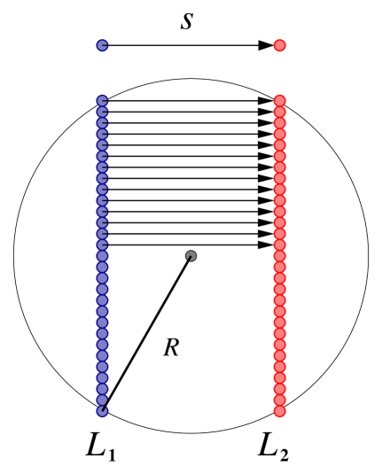
FIG. 1.: Locus of points in separated by a fixed distance $s=|s|\,\hat{x}$ from a line $L_{1}$ in a circle of radius $R$. If $L_{1}$ is the line $x=-s/2$ then $L_{2}$ is the line $x=+s/2$, where $-\left(R^{2}-s^{2}/4\right)^{1/2}\leq y\leq\left(R^{2}-s^{2}/4\right)^{1/2}$.

aaa

aaa

FIG. 2.: (a) Locus of points in a circle of radius $R$ separated by a vector $\vec{s}=s\hat{x}$. For each point $\vec{r}_{1}$ in $A_{1}$, there is a unique point $\vec{r}_{2}$ in $A_{2}$ such that $\vec{s}=\vec{r}_{2}-\vec{r}_{1}$. $A_{2}$ is the overlap between the circle and the region obtained by translating the line $L_{2}$ given by $x=s/2$ to the $+\hat{x}$ direction. $A_{1}$ can be obtained by shifting $A_{2}$ a distance $s$ along the $+\hat{x}$ direction. (b) $A_{3}$ is the overlap between the circle and the region obtained by translating the line $L_{1}$ given by $x=-s/2$ along the $-\hat{x}$ direction. $A_{4}$ can be obtained by shifting $A_{3}$ a distance $s$ along the $\hat{x}$ direction.

aaa

aaa

FIG. 3.: Geometric interpretation of the probability density function $P_{2}(s)$. From Figs. 1 and 2, the probability that two points are separated by a distance $s$ ($\left|\vec{s}\,\right|=\left|s\hat{x}\right|$) in a circle of radius $R$ is proportional to the total shaded area, $A_{3}\bigcup A_{1}\bigcup A_{4}\bigcup A_{2}$ , in the circle $C_{0}$. As can be seen from this figure, this shaded area is given by the overlap of $C_{0}$ with two identical circles $C_{1}$ and $C_{2}$ as shown, where $C_{0}$ is the circle $x^{2}+y^{2}=R^{2}$, $C_{1}$ is $(x-s)^{2}+y^{2}=R^{2}$, and $C_{2}$ is $(x+s)^{2}+y^{2}=R^{2}$.

aaa

aaa

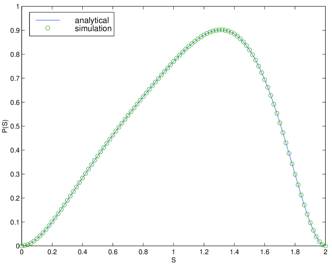
FIG. 4.: PDF for a $3$-dimensional sphere of radius $R=1$ and $\rho\propto r^{2}$.

aaa

aaa

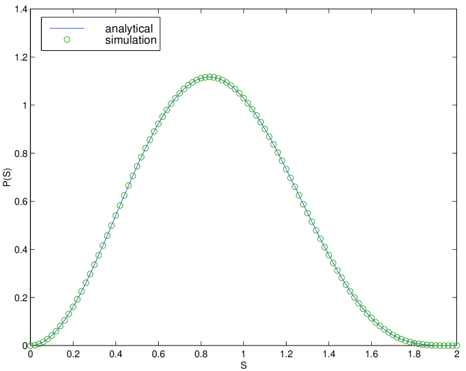
FIG. 5.: PDF for a $3$-dimensional sphere of radius $R=1$ and $\rho\propto 1-r^{2}$.

aaa

aaa

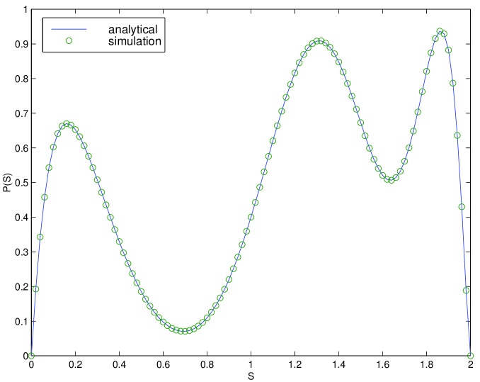
FIG. 6.: Plot of $P_{2}(s)$ as a function of $s$ for a $2$-dimensional circle of radius $R=1$ for the case $\rho\propto x^{4}y^{4}$. See text for further discussion.

aaa

aaa

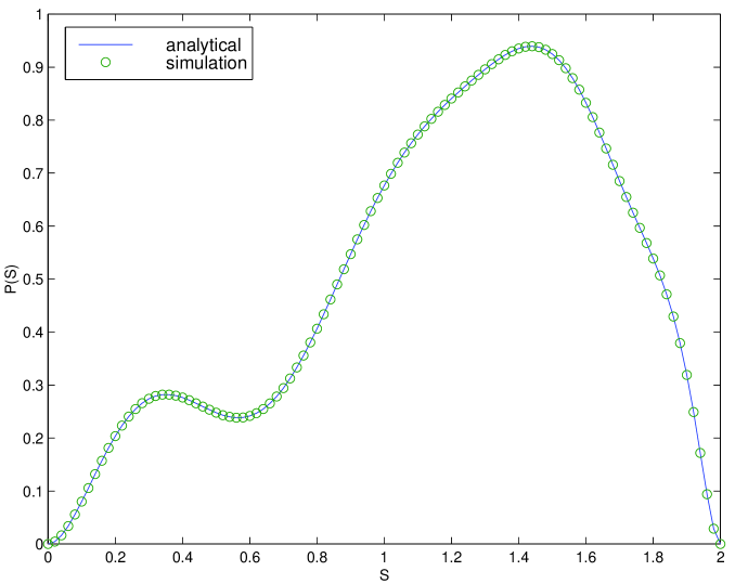
FIG. 7.: Plot of $P_{3}(s)$ as a function of $s$ for a $3$-dimensional sphere of radius $R=1$ and $\rho(x,y,z)=(945N/4\pi)x^{2}y^{2}z^{2}$.

aaa

aaa

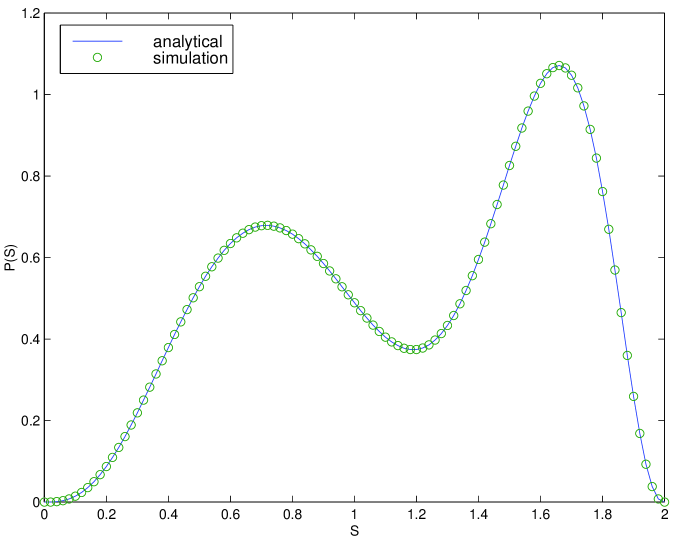
FIG. 8.: Plot of $P_{4}(s)$ as a function of $s$ for a $4$-dimensional hypersphere of radius $R=1$ and $\rho=\left(32N/\pi^{2}\right)x_{1}^{4}$.

aaa

aaa

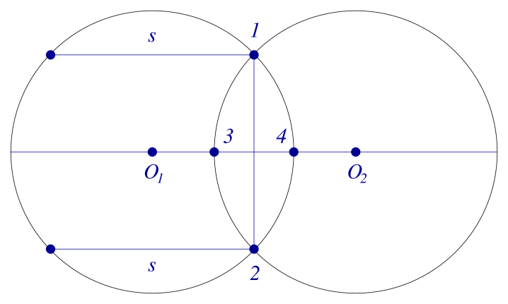
FIG. 9.: A simple diagram showing circle $O_{1}$ and $O_{2}$ are identical with the center of $O_{1}$ located at $(0,0)$ and $O_{2}$ at $(s,0)$.

aaa