General Theory of Lee-Yang Zeros in Models with First-Order Phase Transitions

Abstract

We present a general, rigorous theory of Lee-Yang zeros for models with first-order phase transitions that admit convergent contour expansions. We derive formulas for the positions and the density of the zeros. In particular, we show that for models without symmetry, the curves on which the zeros lie are generically not circles, and can have topologically nontrivial features, such as bifurcation. Our results are illustrated in three models in a complex field: the low-temperature Ising and Blume-Capel models, and the $q$-state Potts model for $q$ large enough.

Almost half a century ago, in two classic papers YL , Lee and Yang studied the zeros of the Ising partition function in the complex magnetic field plane, showed rigorously that the zeros lie on the unit circle, and proposed a program to analyze phase transitions in terms of these zeros. A decade later, Fisher F extended the study of the Ising partition function zeros to the complex temperature plane. Since that time, there have been numerous studies, both exact and numerical, of the Lee-Yang and Fisher zeros in a wide variety of models pool . However, with a few notable exceptions rigorpool , remarkably little progress has been made in extending the rigorous Lee-Yang program. This is due to the fact that rigorous statistical mechanics has relied almost exclusively on probabilistic techniques which fail in a complex parameter space. In this Letter, we adapt complex extensions compPS ; fss ; BBCKK of Pirogov-Sinai theory PSZ to realize the Lee-Yang program in a general class of models with first-order phase transitions.

The purpose of this work is threefold. First, it is of interest to establish the mathematical foundation of a program that has been so central to statistical physics. Second, our theory gives a novel physical interpretation of the existence and position of partition function zeros by relating them to the phase coexistence lines in the complex plane. Finally, from a practical viewpoint, our theory provides a framework for the interpretation of numerical data by allowing explicit, rigorous computation of the position of the zeros. Indeed, we find rigorous results which clarify many ambiguities in published data. Specifically, in models without an underlying symmetry, we prove that the zeros generically do not lie on circles, even in the thermodynamic limit. This applies, in particular, to the Blume-Capel and Potts models in complex magnetic fields; see Lee ; KC for heuristic studies of these models. We also prove that the curves defined by the asymptotic positions of the zeros can have topologically nontrivial features, such as bifurcation and coalescence, and show that these features correspond to triple (or higher) points in the complex phase diagram.

The results to be stated next are rather technical. Roughly speaking, they say that, for models with a convergent contour expansion, the partition function can be written in the form (1) and its zeros are given as solutions to equations (2) and (3). Readers unfamiliar with rigorous expansion techniques are encouraged to see the concrete examples following the main results.

Main Result: Consider a $d$-dimensional lattice model with $n$ equilibrium phases whose interaction depends on a complex parameter $z$. Suppose $d\geq 2$ and that $z$ is in the region (typically, a large disc or the entire ${\mathbb{C}}$) where the model admits a contour representation with strongly suppressed contour weights. Under suitable conditions compPS ; fss ; PSZ , there are complex functions $f_{\ell}=f_{\ell}(z)$, $\ell=1,\dots,n$, such that the partition function in a periodic volume $V=L^{d}$ at inverse temperature $\beta$ can be written as

$$Z^{\text{per}}_{L}=\sum_{\ell=1}^{n}q_{\ell}\,e^{-\beta f_{\ell}V}+{\mathcal{O}}(e^{-L/L_{0}}e^{-\beta fV}).$$ (1)

Here $L_{0}$ is of the order of the correlation length, $f=\min_{k}\Re{\mathfrak{e}}f_{k}$, and $q_{\ell}$ is the degeneracy of the phase $\ell$. Physically, $f_{\ell}$ can be interpreted as metastable free energies with the stability of the $\ell^{\text{th}}$ phase being characterized by the condition $\Re{\mathfrak{e}}f_{\ell}=f$. If $\ell$ is stable, $f_{\ell}$ is just the free energy of the system with boundary condition $\ell$ complfreen . In the region where $\ell$ is not stable, $f_{\ell}$ is constructed as a smooth extension of $f_{\ell}$ from the stable region. Clearly, $f_{\ell}$ depends on the parameters of the model, but not on $L$.

Eq. (1) can be used to locate the zeros of $Z^{\text{per}}_{L}$ analytically. Excluding a neighborhood of size $\delta_{L}\!\sim\!L^{-(d-1)}$ of the triple or higher coexistence points triple and assuming a degeneracy removing condition nondeg , each zero of $Z^{\text{per}}_{L}$ lies within ${\mathcal{O}}(e^{-L/L_{0}})$ of a solution to the equations

$$\Re{\mathfrak{e}}f_{\ell,L}^{\operatorname{eff}}=\Re{\mathfrak{e}}f_{m,L}^{\operatorname{eff}}<\Re{\mathfrak{e}}f_{k,L}^{\operatorname{eff}}\text{ \ for all }k\neq\ell,m,$$ (2)

$$\beta V(\Im{\mathfrak{m}}f_{\ell}-\Im{\mathfrak{m}}f_{m})=\pi\text{ mod }2\pi$$ (3)

for some $\ell\neq m$, where $f_{\ell,L}^{\operatorname{eff}}=f_{\ell}-(\beta V)^{-1}\log q_{\ell}$. In fact, the solutions to (2) and (3) and the zeros of $Z^{\text{per}}_{L}$ are in one-to-one correspondence. As a consequence, the zeros of $Z^{\text{per}}_{L}$ asymptotically concentrate on the phase coexistence curves $\Re{\mathfrak{e}}f_{\ell}=\Re{\mathfrak{e}}f_{m}$ with the density $\frac{1}{2\pi}\beta V|(d/dz)(f_{\ell}-f_{m})|$. Inside the $\delta_{L}$-neighborhood of the multiple coexistence points, both the analysis and the resulting equations for the zeros are more complicated; see BBCKK for details. However, it turns out that all but a uniformly bounded number of zeros (out of the total of order $L^{d}$) can be accounted for by the simple equations (2) and (3).

The proof, which appears elsewhere BBCKK , is technically complicated, but the main idea is simple. The key input is a complex version of methods developed mainly in the context of finite-size scaling PSZ ; compPS ; fss leading to equation (1) and similar expressions for the derivatives of $Z_{L}^{\text{per}}$. Equations (2) and (3) for the zeros of $Z_{L}^{\text{per}}$ arise from “destructive interference” of two terms, $q_{\ell}e^{-\beta f_{\ell}V}$ and $q_{m}e^{-\beta f_{m}V}$, in the sum in (1). Outside the $\delta_{L}$-neighborhood of multiple coexistence points, all other terms are negligible.

To illustrate our result, we will discuss three specific models in the presence of a complex external field.

Ising Model: The nearest-neighbor Hamiltonian is

$$\beta H=-J\sum_{\langle x,y\rangle}\sigma_{x}\sigma_{y}-h\sum_{x}\sigma_{x}.$$

Here $\sigma_{x}\in\{-1,+1\}$, the coupling $J>0$ is taken large enough to ensure absolute convergence of the low-temperature expansion, and $h$ is the complex external field. Neglecting the error term, Eq. (1) becomes

$$Z^{\text{per}}_{L}=e^{-\beta f_{+}V}+e^{-\beta f_{-}V}.$$

This leads to the following equations for the zeros:

$$\Re{\mathfrak{e}}(f_{+}-f_{-})=0$$ (4)

$$\Im{\mathfrak{m}}(f_{+}-f_{-})=\textstyle\frac{(2k-1)\pi}{\beta V},\quad k=1,\dots,V.$$ (5)

Inserting the low-temperature expansions of $f_{\pm}$,

$$\beta f_{\pm}=\mp h-dJ-e^{-4dJ}e^{\mp 2h}+R(\pm h),$$

where $R(h)$ and its derivative are both ${\mathcal{O}}(e^{-4(2d-1)J})$, we find that the zeros occur at $e^{2h}=e^{i\theta_{k}}$, with

$$\textstyle\theta_{k}=\frac{(2k-1)\pi}{V}+2e^{-4dJ}\sin\Bigl{(}\frac{(2k-1)\pi}{V}\Bigr{)}+{\mathcal{O}}\bigl{(}\frac{k}{V}e^{-4(2d-1)J}\bigr{)},$$

$k=1,\dots,V$. Moreover, the $h\leftrightarrow-h$ symmetry can be used to prove that condition (4) is equivalent to $\Re{\mathfrak{e}}\,h=0$, guaranteeing that the zeros of $Z^{\text{per}}_{L}$ lie within an ${\mathcal{O}}(e^{-L/L_{0}})$-neighborhood of the unit circle. The $h\leftrightarrow-h$ symmetry of the partition function then allows us to conclude that, for large $L$, the zeros lie exactly on the unit circle; see the end of the Blume-Capel section for details of an analogous argument. This gives an alternative proof of the Lee-Yang circle theorem at low temperatures BBCKK . We stress that symmetry is the key factor here; in the absence of symmetry, (4) does not in general lead to circles.

Blume-Capel Model: The Hamiltonian BC is

$$\beta H=-\sum_{\langle x,y\rangle}J(\sigma_{x}-\sigma_{y})^{2}-\sum_{x}(\lambda\sigma_{x}^{2}+h\sigma_{x})$$

with spins $\sigma\in\{-1,0,+1\}$, real parameters $J>0$ and $\lambda$, and complex field $h$. For $J$ large, the real $(\lambda,h)$-phase diagram features three phases labeled by $+$, $0$, and $-$, each with an abundance of the corresponding spin.

The zeros of this model are shown in Fig. 1. Note that the zeros have a non-uniform distribution, forming curves of non-circular shape, and that for $\lambda$ in a certain interval $(\lambda_{c}^{-},\lambda_{c}^{+})$, bifurcation (i.e., splitting of the curve) occurs. In the remainder of this section, we rigorously establish these features for large $J$. Before beginning our analysis, we remark that in Lee a phenomenological theory of partition function zeros based on fss was developed and then applied to the Blume-Capel model. In contrast to our approach, that of Lee gives no quantitative estimate of approximations or errors, and it misses certain important qualitative features, namely the bifurcation.

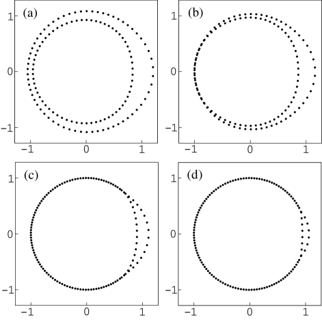
Figure 1: The 128 zeros of the partition function of the Blume-Capel model in the complex $e^{h}$ plane, for the $8\times 8$ periodic square grid at $e^{-4J}=1/{16}$ and $e^{\lambda}=$ (a) $0.9$, (b) $0.94$, (c) $1$, (d) $1.07$. The actual zeros lie within a distance of order $e^{-10J}\!\!+\!e^{-L/L_{0}}$ of those depicted. For $\lambda<\lambda_{c}^{-}\approx-e^{-4J}$, the outer region of the $+$ phase is separated from the inner $-$ phase by an annular region of the $0$ phase (a); asymptotically, the zeros lie on the boundaries of these regions. As $\lambda$ increases through $\lambda_{c}^{-}$, the two boundaries coalesce on the left hand side, leading to bifurcation for $\lambda>\lambda_{c}^{-}$. The common boundary grows (c,d) and, eventually, at $\lambda=\lambda_{c}^{+}\approx e^{-4J}$, the $0$ phase disappears and bifurcation terminates. For $\lambda>\lambda_{c}^{+}$, all zeros lie on the unit circle.

Fix $J$ large and let $e^{h}=z=re^{i\theta}$. Our analysis is done in two steps. First, we focus on the unit circle, $r=1$, and identify $\lambda_{c}^{\pm}$ and the position $e^{\pm i\theta_{c}(\lambda)}$ of the splitting points. Then we extend the analysis to all $r$.

The $J=\infty$ phase diagram has three ground states, $\sigma\equiv-1$, $0$, $1$, with energy densities $-\lambda+h$, $0$, $-\lambda-h$. The large-$J$ expansions of the free energies are

$$e^{-\beta f_{+}} =\!ze^{\lambda}\exp\bigl{\{}{\textstyle\frac{1}{z}}e^{-\lambda-4J}+2{\textstyle\frac{1}{z^{2}}}e^{-2\lambda-6J}+R_{+}(z)\bigr{\}}$$

$$e^{-\beta f_{-}} =\!{\textstyle\frac{1}{z}}e^{\lambda}\exp\bigl{\{}ze^{-\lambda-4J}+2z^{2}e^{-2\lambda-6J}+R_{-}(z)\bigr{\}}$$

$$e^{-\beta f_{0}} =\!\exp\bigl{\{}\!(z\!+\!{\textstyle\frac{1}{z}})e^{\lambda-4J}\!+\!2(z^{2}\!+\!{\textstyle\frac{1}{z^{2}}})e^{2\lambda-6J}\!+\!R_{0}(z)\!\bigr{\}}\!,$$

which, for brevity, we write only for $d=2$ BCfreeen . Here $R_{\pm}(z)$ and $R_{0}(z)$ and their first two derivatives are all ${\mathcal{O}}(e^{-8J})$. There are no phase degeneracies, $q_{0}=q_{\pm}=1$.

By Eq. (2), the analysis of the loci of the zeros requires comparison of $\Re{\mathfrak{e}}f_{+}$, $\Re{\mathfrak{e}}f_{-}$, and $\Re{\mathfrak{e}}f_{0}$. On the unit circle, $\Re{\mathfrak{e}}f_{+}=\Re{\mathfrak{e}}f_{-}$. Thus it suffices to study the sign of $\Delta_{\pm}=$ $\Re{\mathfrak{e}}\beta f_{\pm}-\Re{\mathfrak{e}}\beta f_{0}$. For $|\lambda|\gg e^{-4J}$, $\operatorname{sgn}(\Delta_{\pm})=-\operatorname{sgn}\lambda$. So let $\lambda={\mathcal{O}}(e^{-4J})$. Then, for $J$ large,

$$\Delta_{\pm}=-\lambda+e^{-4J}(2e^{\lambda}\!-\!e^{-\lambda})\cos\theta+{\mathcal{O}}(e^{-6J}),$$ (6)

so that $(d/d\theta)\Delta_{\pm}<0$ for $\theta\in(0,\pi)$ remark and, similarly, $(d/d\lambda)\Delta_{\pm}=-1+{\mathcal{O}}(e^{-4J})$. This implies the existence of $\lambda_{c}^{\pm}=\pm e^{-4J}+{\mathcal{O}}(e^{-6J})$ and $\theta_{c}(\lambda)$, with $\theta_{c}(\lambda)\in(0,\pi)$ for all $\lambda\in(\lambda_{c}^{-},\lambda_{c}^{+})$, such that, on the unit circle, $0$ is the only stable phase for all $\theta$ when $\lambda<\lambda_{c}^{-}$ and for $|\theta|<\theta_{c}(\lambda)$ when $\lambda\in[\lambda_{c}^{-},\lambda_{c}^{+}]$, whereas $\pm$ are the only stable phases in the complementary region of $(\lambda,\theta)$. Moreover, $\theta_{c}(\lambda)$ decreases with $\lambda$ and $\theta_{c}(\lambda)\to 0$ (resp., $\pi$) when $\lambda\uparrow\lambda_{c}^{+}$ (resp., $\lambda\downarrow\lambda_{c}^{-}$).

Now let $r$ be arbitrary. We have $(d/dr)\Re{\mathfrak{e}}f_{\pm}(z)=\pm r^{-1}+{\mathcal{O}}(e^{-4J})$ and $(d/dr)\Re{\mathfrak{e}}f_{0}(z)={\mathcal{O}}(e^{-4J})$. Using the symmetries of the model,

$$\Re{\mathfrak{e}}f_{\pm}(z)=\Re{\mathfrak{e}}f_{\mp}(z^{-1})\quad\text{and}\quad\Re{\mathfrak{e}}f_{0}(z)=\Re{\mathfrak{e}}f_{0}(z^{-1}),$$

it follows that there is a function $\theta\mapsto r(\theta)$, $0\leq 1-r(\theta)\leq{\mathcal{O}}(e^{-4J})$, $r(\theta)=r(-\theta)$, such that $-$ is stable for $r\leq r(\theta)$, $0$ is stable for $r(\theta)\leq r\leq 1/r(\theta)$, and $+$ is stable for $r\geq 1/r(\theta)$. Notice that $r(\theta)=1$ for $|\theta|\geq\theta_{c}(\lambda)$ when $\lambda_{c}^{-}\leq\lambda\leq\lambda_{c}^{+}$ and for all $\theta$ when $\lambda>\lambda_{c}^{+}$.

Consider now $L\gg L_{0}$ and suppose there is a partition function zero at $z_{0}=\rho e^{i\psi}$. If $r(\psi)<1$, then the zero lies close to one of the curves defined by the equations $\Delta_{\pm}=0$. We claim that these curves are non-circular and that the zeros do not maintain a uniform spacing along them. Indeed, set $\lambda=0$ for simplicity and observe that

$$e^{\Delta_{\pm}}=\bigl{|}z^{\mp 1}\exp\bigl{\{}z^{\pm 1}e^{-4J}+2z^{\pm 2}e^{-6J}+{\mathcal{O}}(e^{-8J})\bigr{\}}\bigr{|}.$$

Replacing $z^{\pm 1}$ by $x+iy$, the equation $\Delta_{\pm}=0$ and the expansion of the exponential up to ${\mathcal{O}}(e^{-8J})$ yield

$$x^{2}+y^{2}=1+2xe^{-4J}+4(x^{2}-y^{2})e^{-6J}+{\mathcal{O}}(e^{-8J}).$$

This is an ellipse centered at $e^{-4J}+{\mathcal{O}}(e^{-8J})$ with semiaxes $1\pm 2e^{-6J}+{\mathcal{O}}(e^{-8J})$. To determine the density of zeros, we compute $|(d/dz)(f_{\pm}-f_{0})|$ and easily verify that it is non-constant on the above ellipse.

If, on the other hand, $r(\psi)=1$ triplepoints , then, for $L$ large enough, the zero necessarily lies exactly on the unit circle, $\rho=1$. Indeed, by (2), (3), and the degeneracy removing condition nondeg , the distance between two adjacent zeros is of order $L^{-d}$. But we also have $|\rho-r(\psi)|=|\rho-1|\leq{\mathcal{O}}(e^{-L/L_{0}})$, and if $\rho\not=1$, then by symmetries of the model, there would be another zero at $\bar{z}_{0}^{-1}=\rho^{-1}e^{i\psi}$. However, $|z_{0}-\bar{z}_{0}^{-1}|\leq{\mathcal{O}}(e^{-L/L_{0}})\ll L^{-d}$, a contradiction. A similar argument proves a “local” version of the Lee-Yang theorem class in a large class of models for which the standard, “global” theorem fails.

Potts Model:

The Hamiltonian is

$$\beta H=-J\sum_{\langle x,y\rangle}\delta_{\sigma_{x},\sigma_{y}}-h\sum_{x}\delta_{\sigma_{x},1}.$$ (7)

with spins $\sigma\in\{1,2,\dots,q\}$, real coupling $J>0$, and complex field $h$. For $h=0$ this is the standard Potts model, with a $q$-fold degenerate ordered phase at large $J$ and a disordered phase at small $J$, coexisting at $J_{c}^{q}\approx\frac{1}{d}\log q$. The transition is first-order for large $q$ KS , while it is presumably second order for $q\leq q_{c}(d)$. For $h\neq 0$ and $q$ large, the phase diagram was determined first by formal expansion G , and recently by rigorous probabilistic methods BBCK . The Lee-Yang zeros of (7) were studied numerically in KC , where it was suggested that the zeros lie on almost circular curves slightly outside the unit circle, for $J$ both above and below $J_{c}^{q}$. While, by three-phase coexistence, this turns out to be incorrect for $J<J_{c}^{q}$ (see Fig. 2), we prove that this is indeed the case for $J\geq J_{c}^{q}$, thus resolving a controversy in KC .

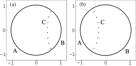
Figure 2: Complex-$e^{h}$ diagram showing the zeros of the Potts model in a three-dimensional periodic box of size $V=1000$ with parameters $q=25$, $e^{3J}/q=$ (a) $1.185$ and (b) $1.155$. In each case, there are 1000 zeros distributed on three non-circular arcs, labeled A, B, and C, with those on A and B denser than those on C. The outer region corresponds to the ordered magnetized phase, while the regions left, resp., right, of arc C contain the ordered non-magnetized and disordered phase. For $V$ large, arc C shows up first at $J=J_{c}^{q}$, it passes through zero at $J=J_{c}^{q-1}$, and it disappears at $J\approx J_{c}^{q-2}$.

The model (7) has three phases: the disordered phase $(D)$ with degeneracy $q_{D}=1$, and two ordered phases: a magnetized $(M)$ and a non-magnetized $(O)$ phase, with degeneracies $q_{M}=1$ and $q_{O}=q-1$, characterized by abundances of $\sigma_{z}=1$ and $\sigma_{z}=\text{const.}\neq 1$, respectively. Let us abbreviate $z=e^{h}$, $\kappa_{d}=d(2d-1)$, $Q_{z}^{(k)}=q-1+z^{k}$, and $Q_{z}=Q_{z}^{(1)}$. The free energies are given BBCK by

$$e^{-\beta f_{D}} =Q_{z}\exp\bigl{\{}d(e^{J}-1)Q_{z}^{(2)}/Q_{z}^{2}+\kappa_{d}(e^{J}-1)^{2}Q_{z}^{(3)}/Q_{z}^{3}-(\kappa_{d}+1/2)(e^{J}-1)^{2}[Q_{z}^{(2)}/Q_{z}^{2}]^{2}+{\mathcal{O}}(1/q^{3-4/d})\bigr{\}}$$

$$e^{-\beta f_{M}} =z\exp\bigl{\{}dJ+e^{-2dJ}(Q_{z}z^{-1}-1)+de^{-(4d-1)J}(Q_{z}^{2}+e^{J}Q_{z}^{(2)})z^{-2}-(d+1/2)e^{-4dJ}Q_{z}^{2}z^{-2}+{\mathcal{O}}(1/q^{3-2/d})\bigr{\}}$$

$$e^{-\beta f_{O}} =\exp\bigl{\{}dJ+e^{-2dJ}(Q_{z}-1)+de^{-(4d-1)J}(Q_{z}^{2}+e^{J}Q_{z}^{(2)})-(d+1/2)e^{-4dJ}Q_{z}^{2}+{\mathcal{O}}(1/q^{3-2/d})\bigr{\}}.$$

The zeros of the periodic Potts partition function are depicted in Fig. 2. In particular, for $J_{-}<J<J_{+}$ (where $J_{+}=J_{c}^{q}$ and $J_{-}\approx J_{c}^{q-2}$), the loci do not lie on a single closed curve but rather split the complex plane into three pieces, corresponding to the regions of stability of the three phases above. The number of zeros on the inner arc is roughly $V/(2\pi q)$, so one needs to take $V$ quite large and tune $J$ to fall inside the narrow window $(J_{-},J_{+})$ to find any interior zeros. This explains why these zeros were not detected in previous numerical work KC .

Despite their appearance, none of the curves in Fig. 2 is a circle. This is verified by finding the coexistence curves (2) for three distinct pairs $k,\ell\in\{D,M,O\}$. When $J\geq J_{c}^{q}$, only the phases $M$ and $O$ are relevant, and the asymptotic location of the zeros is given by $\Re{\mathfrak{e}}f_{O}=\Re{\mathfrak{e}}f_{M}$. For $z=re^{i\theta}$, this easily implies

$$r=1+qe^{-2dJ}(1-\cos\theta)+{\mathcal{O}}(1/q^{2}),$$

so that for $J\geq J_{c}^{q}$ and $V\to\infty$, all zeros with $|\theta|\gg 1/\sqrt{q}$ are asymptotically outside the unit circle. By invoking arguments similar to remark , this extends to all $\theta$ BBCK . There are two finite-volume corrections: an outward shift of order $1/V$ due to $f_{O}>f_{O,L}^{\text{eff}}$ (see Eq. (2)) and an error ${\mathcal{O}}(e^{-L/L_{0}})$ coming from (1). Since $1/V\gg{\mathcal{O}}(e^{-L/L_{0}})$, this proves the initial numerical observation in KC .

To make the interesting features clearly visible, Figs. 1 and 2 were drawn for values of $e^{-4J}$ and $q$ for which we have not proved convergence of our expansions. However, as established above, all the depicted behaviors indeed occur once $e^{-J}$ (or $1/q$) and $e^{-L/L_{0}}$ are small enough.

In summary, we identify the loci of complex zeros with the complex phase coexistence curves. For particular models, we use this identification to map the precise location of these zeros. We find that, in general, the loci are non-uniform and that the resulting curves are non-circular; if more that two phases are present, the curves also have bifurcation (i.e., splitting) points.

The research of R.K. was partly supported by the grant GAČR 201/00/1149.

References

(1)
C.N. Yang, T.D. Lee, Phys. Rev. 87, 404 (1952);
T.D. Lee, C.N. Yang, ibid.87, 410 (1952).
(2)
M.E. Fisher, in Lectures in Theoretical Physics, vol 7c,
edited W.E. Brittin (University of Colorado Press, Boulder, 1965) p. 1.
(3)
For recent references see e.g.: Lee ; KC ;
W.T. Lu, F.Y. Wu, Physica A258, 157 (1998);
C.-N. Chen, C.-K. Hu, F.Y. Wu, Phys. Rev. Lett. 76, 169 (1996);
etc.
(4) see e.g.:
D. Ruelle, Phys. Rev. Lett. 26 303 (1971); E.H. Lieb,
A.D. Sokal, Commun. Math. Phys. 80 153 (1981); A.D. Sokal,
cond-mat/9904146.
(5)
C. Borgs, J. Imbrie, Commun. Math. Phys. 123, 305 (1989);
K. Gawȩdzki, R. Kotecký, A. Kupiainen, J. Stat. Phys. 47, 701
(1987).
(6) C. Borgs, R. Kotecký,
J. Stat. Phys. 61, (1990) 79; Phys. Rev. Lett. 68,
(1992) 1734; C. Borgs, R. Kotecký, S. Miracle-Solé, J. Stat.
Phys., 62, 529 (1991); C. Borgs, W. Janke, Phys. Rev. Lett.
68, 1738 (1992).
(7)
M. Biskup, C. Borgs, J.T. Chayes, L.J. Kleinwaks, R. Kotecký,
unpublished.
(15)
Here, in the first line, comes from the energy
density of the ground state, whereas the first term in the
exponential accounts for single-spin flips with
energy cost . The second term in the exponential
comes from simultaneous flips of nearest
neighbors ( accounts for the orientations of the pair). Similar
reasoning applies to . The ground state admits both
flips in its lowest excitations, leading to the
terms and in the third line.
(16)
Indeed, by (6), this is true outside an neighborhood of and . At these points,
by symmetry. Since
(resp., ) in a neighborhood of (resp., ),
is strictly decreasing (increasing) there,
which proves the claim.
(17)
More precisely, we need that for
.
(18)
Our local theorem requires that, in an -neighborhood
of some with , (i)
maximally two phases are stable, (ii) the phases are related by
the symmetry, and (iii) they coexist on a
curve in . Then in , and all zeros in with lie on the
unit circle. See BBCKK .