DFTT 63/99

Matrix strings from generalized Yang-Mills theory on arbitrary Riemann surfaces.

M. Billó^a, A. D’Adda^a and P. Provero^b,a

^a Dipartimento di Fisica Teorica dell’Università di Torino and

Istituto Nazionale di Fisica Nucleare, Sezione di Torino

via P.Giuria 1, I-10125 Torino, Italy

^b Dipartimento di Scienze e Tecnologie Avanzate

Università del Piemonte Orientale

I-15100 Alessandria, Italy

We quantize pure 2d Yang-Mills theory on an arbitrary Riemann surface in the gauge where the field strength is diagonal. Twisted sectors originate, as in Matrix string theory, from permutations of the eigenvalues around homotopically non-trivial loops. These sectors, that must be discarded in the usual quantization due to divergences occurring when two eigenvalues coincide, can be consistently kept if one modifies the action by introducing a coupling of the field strength to the space-time curvature. This leads to a generalized Yang-Mills theory whose action reduces to the usual one in the limit of zero curvature. After integrating over the non-diagonal components of the gauge fields, the theory becomes a free string theory (sum over unbranched coverings) with a U$(1)$ gauge theory on the world-sheet. This is shown to be equivalent to a lattice theory with a gauge group which is the semi-direct product of $S_{N}$ and U$(1)^{N}$. By using well known results on the statistics of coverings, the partition function on arbitrary Riemann surfaces and the kernel functions on surfaces with boundaries are calculated. Extensions to include branch points and non-abelian groups on the world-sheet are briefly commented upon.

1 Introduction

The solution of pure two-dimensional Yang-Mills theory (YM2 in the following) on a general Riemann surface has been known for some time. It was obtained on the lattice in [1, 2], and in the continuum in [3, 4, 5]. For instance, the partition function of the U$(N)$ theory on a surface of genus $G$ and area ${\cal A}$ is

$$Z=\sum_{R}(d_{R})^{2-2G}\,{\rm e}^{-{1\over 2}g^{2}{\cal A}\,C_{R}}~{},$$ (1)

where the sum runs on the irreducible representations $R$, of dimension $d_{R}$ and quadratic casimir $C_{R}$, of the U$(N)$ group.

This solution allowed Gross and Taylor [6] to describe the U$(N)$ YM2 theory, in the large $N$ limit, as a particular type of string theory. In fact they could show that in this limit the partition function (1) counts distinct maps from world-sheets of genera $g$ to the target space represented by the base manifold of genus $G$.

Recently, a different way to formulate YM2 on a torus or a cylinder as a string theory has been suggested [7, 8], and in this paper we are going to extend this formulation to arbitrary Riemann surfaces. This proposal is inspired by Matrix string theory [9, 10]. In Matrix string theory one considers the ${\cal N}=8$ supersymmetric YM2 theory, defined on a cylinder. This theory contains eight scalar fields $X_{M}$ with their supersymmetric partners $\Theta_{\alpha}$ in the adjoint representation of the U$(N)$ gauge group. In the limit $g_{\rm YM}\to\infty$ all these fields commute and can be simultaneously diagonalized. The $N$ eigenvalues of $X_{M}$ take the role of the eight transverse coordinates describing the world-sheets of a gas of free superstrings. The eigenvalues, however, can be subjected to a permutation as one goes around the compact direction of the cylinder, giving rise to twisted sectors in correspondence with the conjugacy classes of the symmetric group $S_{N}$. Strings of different lengths are present in each sector, and correspond to the cycles of the permutation.

In [7] we showed that twisted sectors appear naturally in pure YM2 on a torus or a cylinder if one chooses the so-called unitary gauge [11], namely the gauge in which the field strength is diagonal. Their inclusion leads to a partition function that is different from the standard one of [2], has a richer structure and is closely related to the partition function of the whole matrix string theory [12, 13].

However, in higher genus Riemann surfaces there are always divergences associated to the twisted sectors in correspondence of points where two eigenvalues of the field strength coincide. A rather ad hoc regularization was suggested in [5], whose effect is to suppress all non-trivial sectors in order to reproduce the standard result.

We propose here to study a generalized YM2 (in the sense of [14, 15]) in which such divergences do not occur, and the twisted sectors can be consistently kept into account. This can be achieved by introducing a suitable coupling of the field-strength to the Riemann curvature of the space-time manifold. The action of the generalized theory reduces to the one of ordinary YM2 for flat surfaces. In the generalized theory the twisted sectors are in one-to one correspondence with the unbranched $N$-coverings of the surface, and the original U$(N)$ gauge group reduces to an abelian gauge group for each connected component of the covering. For the torus and the cylinder the results of [7] are reproduced. All previous results are discussed in Sections 2 and 3. In Section 4 we show that, after integration over the non Cartan components of the gauge fields, the theory can be described as a lattice gauge theory of a group ${\cal G}_{N}$ defined as the semi-direct product of $S_{N}$ and U$(1)^{N}$. By using known results on the statistics of coverings [6, 16], we derive in Sections 5 and 6 the expression for the partition function on surfaces without boundaries and the kernel function for surfaces with an arbitrary number of boundaries. In Section 7, with the conclusions, we outline the main features of the extension of the present theory to the case of interacting strings (branched coverings) and to strings with a non-abelian gauge group on the world-sheet.

2 Unitary gauge and Matrix string theory

Consider a two-dimensional gauge theory defined on a Riemann surface ${\cal M}$, with or without boundaries, and with gauge group ${\cal G}$, for instance U$(N)$. Assume that the theory contains at least one field $F$ transforming in the adjoint representation of ${\cal G}$; in the case of U$(N)$, $F$ is a $N\times N$ hermitian matrix. A possible gauge choice consists in choosing $F$ with values in the Cartan subalgebra of ${\cal G}$, that is, in the U$(N)$ case, in choosing $F$ diagonal (unitary gauge). In fact it is always possible at each point $x$ of ${\cal M}$ to find a gauge transformation $g(x)$ that casts $F$ into a diagonal form:

$$g^{-1}(x)F(x)g(x)={\rm diag}(\lambda(x))~{}.$$ (2)

Such gauge fixing is not complete as it leaves a U$(1)^{N}$ gauge invariance, and is affected by Gribov ambiguities because at each point $x$ there are in general $N!$ different gauge-fixed forms of $F$, related to each other by arbitrary permutations of the eigenvalues:

$$Q^{-1}\lambda_{i}(x)Q=\lambda_{Q(i)}(x)~{}.$$ (3)

As a consequence of the Gribov ambiguity it is not possible in general to put $F$ in diagonal form globally, namely on the whole ${\cal M}$ without discontinuities. In fact if we map ${\cal M}$ into a polygon with pairs of edges suitably identified, and fix the unitary gauge on the polygon (this is always possible as the bundle is trivial on a disc), after gauge fixing the eigenvalues of $F$ will in general appear in a different order on the edges that are to be identified.

More precisely: consider a point $x$ on ${\cal M}$, and let $\Pi_{1}(x|{\cal M})$ be the homotopy group on ${\cal M}$ with base point $x$. Let us order the eigenvalues of $F$ in $x$ in an arbitrary way, for instance

$$\lambda_{1}(x)>\lambda_{2}(x)>....>\lambda_{N}(x)~{}.$$ (4)

This will be referred to in the rest of the paper as the standard order. Consider now a non trivial element $\gamma_{x}$ of $\Pi_{1}(x|{\cal M})$, that is a homotopically non-trivial loop starting from $x$. As we go round the loop the eigenvalues of $F$ are subjected to a permutation, or, for a generic gauge group, they are acted upon by an element of the Weyl group. This defines a homomorphism that associates to each element $\gamma_{x}$ of the homotopy group $\Pi_{1}(x|{\cal M})$ an element $P(\gamma_{x})$ of the Weyl group.

The permutation $P(\gamma_{x})$ depends on the choice of the base point $x$ according to the formula

$$P(\bar{\gamma}_{y})=P(\gamma^{-1}_{y\rightarrow x})P(\gamma_{x})P(\gamma_{y\rightarrow x})~{},$$ (5)

where $\bar{\gamma}_{y}$ is a closed loop starting in $y$ and defined by $\bar{\gamma}_{y}=\gamma^{-1}_{y\rightarrow x}\gamma_{x}\gamma_{y\rightarrow x}$ where $\gamma_{y\rightarrow x}$ is an arbitrarily chosen path from $y$ to $x$. $P(\gamma_{y\rightarrow x})$ is the permutation of the eigenvalues in $x$ with respect to the standard order defined above obtained by starting with the eigenvalues in the standard order in $y$ and moving to $x$ along the chosen path $\gamma_{y\rightarrow x}$. Eq. (5) shows that changing the base point of the homotopy group, namely deforming the original path $\gamma_{x}$ into $\bar{\gamma}_{y}$, corresponds to a conjugacy transformation on $P(\gamma_{x})$.

According to this analysis the functional integral over the field configurations of $F$ splits into several topological sectors, one for each homomorphism of $\Pi_{1}(x|{\cal M})$ into $S_{N}$.

It is easy to see that in the case of U$(N)$, where the eigenvalues of $F$ are real and the Weyl group is the symmetric group $S_{N}$, the homomorphic maps of $\Pi_{1}(x|{\cal M})$ into $S_{N}$ are in one-to-one correspondence with the $N$-coverings of ${\cal M}$ without foldings or branch points. In this correspondence each eigenvalue of $F$ is associated to one sheet of the $N$-covering. Such coverings are not in general connected but consist of a certain number of connected parts. The decomposition of a covering into its connected parts coincides with the decomposition of the representations of $\Pi_{1}(x|{\cal M})$ into its irreducible subspaces. A connected part that covers ${\cal M}$ $k$ times consists of a $k$-dimensional subspace of the $N$-dimensional space of the eigenvalues of $F$. This subspace is invariant under the action of $\Pi_{1}(x|{\cal M})$ and does not contain any lower dimensional invariant subspace.

Each connected part can be thought of as the world-sheet of a two-dimensional string that covers $k$ times the target space and that can be described as follows. Let us denote by $\xi_{\alpha}$ ($\alpha=1,2$) a set of coordinates parameterizing the world-sheet. Each point $x$ of the target space has $k$ images on the world-sheet labeled by $\xi_{\alpha,i}(x)$ with $i=1,2,\dots,k$. So we can associate to each point of the world-sheet a single eigenvalue $\lambda(\xi)$ by requiring

$$\lambda(\xi_{i}(x))=\lambda_{i}(x)~{}.$$ (6)

In the end we have a single eigenvalue and a U$(1)$ gauge invariance associated to each connected part of the covering, namely to each irreducible part of the representation of $\Pi_{1}(x|{\cal M})$ in terms of elements of $S_{N}$.

We may be tempted to conclude that, through the mechanism outlined above, a non abelian gauge theory in two dimensions can be described in terms of a string theory with an abelian gauge theory on its world-sheet. However this is true only if the abelianization is not spoiled by other terms in the action that induce a coupling between different sheets of the covering. Therefore we have to require that, at least in some limit for the coupling constants, the strings described above are free or weakly coupled.

In this respect a problem arises directly from the gauge fixing procedure. Indeed, the Faddeev-Popov determinant for our gauge choice induces a strong interaction between different sheets of the covering. In fact, the functional integration measure produces, as usual, a squared Vandermonde determinant of the eigenvalues of $F$:

$${\cal D}F(x)={\cal D}\lambda(x)\prod_{x}\Delta(\lambda)^{2}={\cal D}\lambda(x)\exp\left\{2\int d\mu\sum_{i>j}\log|\lambda_{i}(x)-\lambda_{j}(x)|\right\}~{},$$ (7)

where $d\mu=d^{2}x\sqrt{g}$ is the area element. This term is singular when two eigenvalues coincide and indeed it describes an interaction of different world-sheets (i.e. eigenvalues) at the same target space point $x$. Therefore we must require that the Vandermonde determinants arising from the gauge fixing are exactly canceled for the string picture outlined above to make sense.

This is obtained in Matrix string theories (DVV) [9, 10] by use of supersymmetry. In the limit of vanishing string coupling, the adjoint scalars $X_{M}$ and fermions $\Theta_{\alpha}$ of the theory commute with each other and it is possible to choose a gauge in which they are all diagonal. However no Vandermonde determinant arises from the Faddeev-Popov procedure because contributions from $X_{M}$ and $\Theta_{\alpha}$ cancel exactly.

In [7, 8] we showed that the same cancellation of Vandermonde determinants occurs in pure two-dimensional Yang-Mills theory on a torus or a cylinder if the gauge where the field strength $F$ is diagonal is chosen. The ensuing theory has matrix string states, just as the DVV model, and its partition function is closely related to the one of the DVV model itself [12, 13]. In this paper we show that the results of [7, 8] can be extended to include Riemann surfaces of arbitrary genus and arbitrary number of borders, if one considers a particular generalized Yang-Mills theory (in the sense of [14, 15]) which has the property to coincide with ordinary YM2 on flat surfaces. For the generalized theory it is shown that the cancellation of the Vandermonde determinants occurs also on arbitrary Riemann surfaces and that the theory is consistently described by a string theory with a U$(1)$ gauge symmetry on its world-sheet.

3 Generalized Yang-Mills theory in the unitary gauge

We begin by considering the partition function of a generalized YM2 on an arbitrary Riemann surface [4, 14, 15]. We shall then proceed to fix the gauge in which $F$ is diagonal by following essentially Ref. [11], where the partition function for ordinary YM2 was calculated in the same gauge. The partition function is given by

$$Z({\cal M})=\int{\cal D}A{\cal D}F\exp\left\{-\int_{\cal M}d\mu\,V(F)+{\rm i}\,{\rm tr}\int_{\cal M}f(A)F\right\}~{},$$ (8)

where $d\mu$ is the volume form on $\cal M$ and $f(A)$ is given by

$$f(A)=dA-{\rm i}A\wedge A~{}.$$ (9)

In Eqs. (8) and (9) $F$ is a $N\times N$ hermitian matrix and $A$ is a one-form on $\cal M$ with values in the space of hermitian matrices. $V(F)$ denotes an arbitrary gauge invariant potential, namely a potential that depends only on the eigenvalues of $F$, with in principle an arbitrary dependence from the two-dimensional metric of the surface. In order to reproduce ordinary YM2 it is enough to choose

$$V(F)=\frac{g^{2}_{\rm YM}}{2}{\rm tr}F^{2}$$ (10)

and perform the quadratic functional integral in $F$.

Our gauge choice consists in conjugating the $N\times N$ hermitian matrix $F$ into a diagonal form, namely into its Cartan sub-algebra. As discussed in the previous section, this can always be done locally, according to Eq. (2). The gauge fixed action, including the appropriate Faddeev-Popov ghost term, can be written as the sum of two terms:

$$S_{\rm BRST}({\cal M},t)=S_{\rm Cartan}+S_{\rm off-diag}~{},$$ (11)

where $S_{\rm Cartan}$ involves the diagonal part of $A_{\mu}$ and exhibits the residual U$(1)^{N}$ gauge invariance:

$$S_{\rm Cartan}=\int_{\cal M}\left[V(\lambda)d\mu-\sum_{i=1}^{N}{\rm i}\lambda_{i}dA^{(i)}\right]~{},$$ (12)

where $A^{(i)}$ is the $i$-th diagonal term of the matrix form $A$. The Faddeev-Popov ghost term and the off-diagonal part of $A$ are contained in $S_{\rm off-diag}$ which can be cast into the following form:

$$S_{\rm off-diag}=\int_{\cal M}d\mu\sum_{i>j}(\lambda_{i}-\lambda_{j})\left[\frac{1}{2}\epsilon^{ab}\hat{A}_{a}^{ij}\hat{A}_{b}^{ji}+{\rm i}(c^{ij}\bar{c}^{ji}+\bar{c}^{ij}c^{ji})\right]~{},$$ (13)

where $\hat{A}_{a}^{ij}$ is given by

$$\hat{A}_{a}^{ij}=E_{a}^{\mu}A_{\mu}^{ij}$$ (14)

and $E_{a}^{\mu}$ denotes the inverse of the two-dimensional vierbein. The fields $c^{ji}$ and $\bar{c}^{ij}$ are respectively the ghost and anti-ghost fields associated to the gauge condition $F^{ij}=0$.

The action (13) contains the same number of fermionic and bosonic degrees of freedom and it is invariant, for each value of the composite index $[ij]$, with respect to a set of symmetry transformation with Grassmann-odd parameters which are reported in [7]. One would expect, as a result of these “supersymmetries”, a complete cancellation of the bosonic and fermionic contributions in the partition function. However this supersymmetry is broken on a generic Riemann surface by the measure of the functional integral. The reason is that the supersymmetric partners of the ghost and anti-ghost fields are the zero-forms $\hat{A}_{a}^{ij}$, which are the components of the one-form $A$ in the base of the vierbein (14). So if the measure of the functional integral contains the one-form $A^{ij}$, namely is ${\cal D}A_{\mu}^{ij}{\cal D}c^{ij}{\cal D}\bar{c}^{ij}$, there is a mismatch in the number of bosonic and fermionic degrees of freedom as on a curved surface the “number” of zero-forms and one-forms does not coincide. This results into an anomaly that was explicitly calculated in [11]:

$$\int\prod_{i>j}{\cal D}c^{ij}{\cal D}\bar{c}^{ij}{\cal D}A_{\mu}^{ij}e^{-S_{\rm off-diag}}=\exp\left\{{1\over 8\pi}\int_{\cal M}d\mu R\sum_{i>j}\log|\lambda_{i}-\lambda_{j}|\right\}~{}.$$ (15)

After integration over the non-Cartan fields, the theory becomes purely abelian with a U$(1)^{N}$ gauge symmetry. Taking into account (15), it is described by the effective action

$$S_{\rm eff}=\int_{\cal M}\left[\tilde{V}(\lambda)d\mu-\sum_{i=1}^{N}{\rm i}\lambda_{i}dA^{(i)}\right]~{},$$ (16)

where $\tilde{V}(\lambda)$ is given by

$$\tilde{V}(\lambda)=V(\lambda)-\frac{1}{8\pi}R\sum_{i>j}\log|\lambda_{i}-\lambda_{j}|~{}.$$ (17)

The anomaly term at the r.h.s. of (17) is divergent when two eigenvalues coincide and requires some regularization procedure. In [11], the calculation of the functional integral for the U$(1)^{N}$ theory was done and it turned out to be equivalent to replacing each eigenvalue $\lambda_{i}(x)$ with an arbitrary constant integer value: $\lambda_{i}(x)\rightarrow n_{i}$, where $n_{i}$ is the flux of the abelian field strength. In this way the anomaly term correctly reproduces the dependence of the standard partition function [2, 3, 5] from the genus $G$ of ${\cal M}$, namely the factor $\prod_{i>j}(n_{i}-n_{j})^{2-2G}$. However while in other gauges [5] and in the lattice formulation the integers $n_{i}$, being labels of irreducible representations of U$(N)$, satisfy the condition $n_{1}>n_{2}>n_{3}>...>n_{N}$, in the unitary gauge nothing seems to forbid the existence of “non regular terms”, namely of terms with at least two such integers coinciding.

Non regular terms, which are divergent for $G>1$, were eliminated by a rather ad hoc regularization procedure in [11], leaving the problem of a completely consistent derivation of the standard partition function of YM2 in the unitary gauge still open. It should be noticed that all non trivial maps $\Pi_{1}(x|{\cal M})\rightarrow S_{N}$ lead to sectors made entirely by non regular terms; in fact in a non trivial sector at least two eigenvalues must belong to the same connected world-sheet and, being constant, have to coincide. So any regularization scheme that sets to zero the non regular terms also disregards all sectors corresponding to non trivial maps $\Pi_{1}(x|{\cal M})\rightarrow S_{N}$ .

As already pointed out in [7], non regular terms are finite in the case of the torus ($G=1$), and for any surface with zero curvature the anomaly term at the r.h.s. of Eq. (17) vanishes. In this case no regularization is needed and there is no reason to neglect the non trivial maps in $\Pi_{1}(x|{\cal M})\rightarrow S_{N}$, which for $G=1$ are labeled by pairs $(Q_{1},Q_{2})$ of commuting permutations. The calculation was done by the authors of [7], initially with the hope that the sum over the non trivial maps would just amount to cancel the non regular terms. Surprisingly this happens only if the sum is restricted to the subset of sectors with say $Q_{2}={\bf 1}$, while the entire sum leads to a partition function [7] that has a wider spectrum than the standard one, and which is closely related to the partition function of the DVV string matrix model [12, 13].

Higher genus surfaces and coupling to gravity

In this paper we take a stronger point of view and argue that non-trivial sectors can be consistently kept also on space-times ${\cal M}$ of genus $G>1$. Our point of view can be summarized as follows:

1. Quantization in the unitary gauge beyond the $G=1$ case would ask for a consistent regularization scheme (yet to be found) to cancel the logarithmic singularities in the anomaly term at the r.h.s. of Eq. (17). We propose instead to achieve the same result by modifying the potential $V(\lambda)$ to include in it a term that cancels exactly the divergent anomaly term so that the effective potential $\tilde{V}(\lambda)$ is regular and of the form

   $$\tilde{V}(\lambda)=\sum_{i=1}^{N}v(\lambda_{i})~{},$$ (18)

   with

   $$v(\lambda)=\sum_{k=1}^{\infty}t_{k}\lambda^{k}~{}.$$ (19)

   In this way we define a generalized YM2 theory whose action reduces to the one of standard YM2 in the limit of zero curvature and with a potential $v(\lambda)=\frac{g^{2}_{\rm YM}}{2}\lambda^{2}$. In other words: we consider a generalized YM2 theory which is the ordinary YM2 with a non standard coupling to gravity.

2. It is possible, in our opinion, that the one presented above is the only consistent way to quantize YM2 in the unitary gauge. If that is the case the unitary gauge is not a mere gauge choice, but it defines an entirely new theory. Some possible reasons for it are discussed below.

The redefinition of the potential exactly corresponds to the cancellation of the anomaly. So it is natural to ask: is it possible to define the theory from the beginning in such a way that the fermionic symmetry of (13) is not broken by the integration measure? The obvious answer is to use the zero-forms $\tilde{A}^{ij}_{a}$ rather than $A^{ij}_{\mu}$ as the independent degrees of freedom in the functional integration measure, which becomes ${\cal D}\tilde{A}^{ij}_{a}{\cal D}c^{ij}{\cal D}\bar{c}^{ij}$. This amounts to consider the gauge fields as defined in the tangent space, like spinors, when space-time is curved. In spite of the fact that Eq. (14) is locally invertible this results into a different counting of degrees of freedom. This is apparent in a lattice formulation. Consider a discretized manifold made of squares with sides all of the same length. The ghost and anti-ghost fields sit on the sites of the lattice and the gauge fields on the links. On a site $j$ where the coordination number $c_{j}$ is 4 (zero curvature) the gauge degrees of freedom match exactly the number of degrees of freedom of the ghost anti-ghost system, otherwise the mismatch is proportional to $c_{j}-4$, namely to the curvature. This argument provides a lattice based derivation of Eq. (15). With the gauge fields defined on the tangent space, instead, the degrees of freedom at each site coincide with the one in flat space irrespective of the curvature and no anomaly arises.

We do not know yet how to formulate on a lattice (for instance in the framework of Regge calculus) the coupling to gravity of gauge fields associated to the tangent space. On the other hand, there are indications that ordinary lattice gauge theory might be inadequate in curved space-time. Consider for instance the standard Wilson action: the plaquette variable $U_{\rm pl}$ carries no information about the metric and hence its continuum limit can only depend on quantities that can be written as differential forms, namely

$$U_{\rm pl}\sim{\bf 1}+F_{\mu\nu}dx^{\mu}dx^{\nu}~{}.$$ (20)

However the Lagrangian density $F_{\mu\nu}F_{\rho\sigma}g^{\mu\rho}g^{\nu\sigma}\sqrt{g}$ has a non trivial dependence on the metric and it can be written in the language of differential forms only by using the Hodge dual operator. Therefore the coupling of gauge theories to gravity on a lattice seems to require, instead of the traditional Wilson action, a first order formalism (see for instance [18]) where the plaquette variable is coupled with an auxiliary field which in generic space-time dimensions is an antisymmetric tensor $F_{ab}$, that is a two-form, in the tangent space indices.

Effective action

With the effective potential $\tilde{V}(\lambda)$ given by Eqs. (18) and (19) the action (16) reduces to the sum of $N$ decoupled U$(1)$ theories, namely

$$S_{eff}=\sum_{i=1}^{N}\int\left(v(\lambda_{i})-{\rm i}\lambda_{i}dA^{(i)}\right)~{}.$$ (21)

In the functional integral, however, one has to sum over all sectors corresponding to the homomorphisms $\Pi_{1}(x|{\cal M})\rightarrow S_{N}$, as discussed in the previous section. So in a non trivial sector the U$(1)$ theories in (21) are coupled by the boundary conditions:

$$\gamma~{}~{}:~{}~{}\lambda_{i}(x)\rightarrow\lambda_{P_{\gamma}(i)}(x)~{},$$ (22)

where $\gamma$ is an element of $\Pi_{1}(x|{\cal M})$ and $P_{\gamma}$ the corresponding element of $S_{N}$ in the homomorphism. As a result, rather than $N$ decoupled U$(1)$ theories, we have a U$(1)$ theory on each connected part of the world-sheet, whose area is an integer multiple $k$ of the area ${\cal A}$ of the target space. To each connected world-sheet is associated a U$(1)$ partition function, given by:

$$Z_{{\rm U}(1)}(k{\cal A})=\sum_{n=-\infty}^{+\infty}{\rm e}^{-k{\cal A}v(n)}~{},$$ (23)

where $v(n)$ is given by Eq. (19). Given a covering of ${\cal M}$ with $s_{k}$ ($\sum_{k}ks_{k}=N$) connected parts of area $k{\cal A}$, its contribution to the partition function is then given by

$$Z_{\{s_{k}\}}=\prod_{k=1}^{\infty}\left[Z_{{\rm U}(1)}(k{\cal A})\right]^{s_{k}}~{}.$$ (24)

The total partition function is then obtained by summing (24) over all coverings.

If the surface ${\cal M}$ has boundaries, the states on the $A$-th boundary $\gamma_{A}$ are characterized by the conjugacy class of $P(\gamma_{A})$, namely by the lengths of the cycles of $P(\gamma_{A})$, and by the U$(1)$ holonomies for each cycle of $P(\gamma_{A})$. If $\theta$ is the sum of the U$(1)$ holonomies of all cycles on a given connected world-sheet, the U$(1)$ partition function (23) is replaced by the kernel:

$$K_{{\rm U}(1)}(k{\cal A},\theta)=\sum_{n=-\infty}^{+\infty}{\rm e}^{-k{\cal A}v(n)+{\rm i}n\theta}.$$ (25)

The kernel associated to a surface with an arbitrary number of boundaries is obtained by summing over all coverings with the prescribed conjugacy classes of $S_{N}$ on the boundaries, each covering being weighted with the product of the U$(1)$ kernel functions (25) associated to its connected parts.

In conclusion, after integration on the non-Cartan degrees of freedom, the resulting effective theory is a string theory (theory of coverings without branch points) with a U$(1)$ gauge theory on the world-sheet. In the next section we shall show that this can be described as a lattice gauge theory, with a gauge group ${\cal G}_{N}$ which is the semi-direct product of $S_{N}$ and U$(1)^{N}$.

4 Lattice formulation of the effective theory

Let us consider a surface $\cal M$ with the topology of a disc. Since the homotopy group of the disc is trivial, only the identical permutation can be associated to the boundary of the disc and the only covering consists of $N$ disconnected copies of the disc. According to the previous discussion the kernel on a disc is then given by

$$K\left((P,\varphi),{\cal A}\right)=\delta(P)\sum_{n_{i}}\exp\left\{\sum_{i=1}^{N}\left({\rm i}n_{i}\varphi_{i}-{\cal A}v(n_{i})\right)\right\}~{},$$ (26)

where ${\cal A}$ is the area of the disc and $\varphi_{i}$ the invariant angles of the U$(1)$ holonomies. The kernel is vanishing for any permutation $P$ other than the identity. Consider now the group ${\cal G}_{N}$ defined as the subgroup of U$(N)$ given by the matrices of the form

$$(P,\varphi)={\rm diag}\left(e^{{\rm i}\varphi_{1}},\dots,e^{{\rm i}\varphi_{N}}\right)\;P~{},$$ (27)

where $\varphi_{k}$ are real and $P$ is a permutation matrix:

$$P_{ij}=\delta_{iP(j)}~{}.$$ (28)

Note that with this definition we have $(PQ)_{ij}=\delta_{i\;P\circ Q(j)}$, while on a $N$-vector $\varphi$ we have $(P\varphi)_{i}=\varphi_{P^{-1}(i)}$. The product in ${\cal G}_{N}$ is the ordinary matrix product: in the notation of Eq. (27) the group product reads

$$(P,\varphi)\;(Q,\theta)=(PQ,\varphi+P\theta)~{},$$ (29)

where it is clear that ${\cal G}_{N}$ can be viewed as a semi-direct product of $S_{N}$ and U$(1)^{N}$. The inverse of a group element is given by

$$(P,\varphi)^{-1}=(P^{-1},-P^{-1}\varphi)~{}.$$ (30)

The kernel on a disc $K\left((P,\varphi),{\cal A}\right)$ is invariant under gauge transformations of ${\cal G}_{N}$. In fact from

$$(Q,\theta)(P,\varphi)(Q,\theta)^{-1}=(QPQ^{-1},\theta+Q\varphi-QPQ^{-1}\theta)$$ (31)

it follows almost immediately that

$$K\left((Q,\theta)(P,\varphi)(Q,\theta)^{-1},{\cal A}\right)=K\left((P,\varphi),{\cal A}\right)~{}.$$ (32)

This property will enable us to formulate the theory described in the previous section as a gauge theory of ${\cal G}_{N}$ on a lattice. In fact suppose to draw on the target space ${\cal M}$ a lattice and to associate to each link $\alpha$ an element $(P_{\alpha},\varphi_{\alpha})$ of ${\cal G}_{N}$. The product of all the elements of ${\cal G}_{N}$ along a plaquette defines the plaquette variable $(P_{\rm pl},\varphi_{\rm pl})$ and the partition function is defined as

$$Z_{\rm latt}=\prod_{\alpha}\sum_{P_{\alpha}}\int_{0}^{2\pi}d\varphi_{\alpha}\prod_{\rm pl}K\left((P_{\rm pl},\varphi_{\rm pl}),{\cal A}_{\rm pl}\right)~{}.$$ (33)

As in the case of the heat-kernel action for a U$(N)$ gauge theory, the Boltzmann weight for a single plaquette is left invariant in form if one sews two plaquettes together by integrating over their common link. In fact a straightforward calculation gives:

$$\sum_{Q\in S_{N}}\int\prod_{i}\frac{d\theta_{i}}{2\pi}K\left((P_{1},\varphi_{1})(Q,\theta),{\cal A}_{1}\right)K\left((Q,\theta)^{-1}(P_{2},\varphi_{2}),{\cal A}_{2}\right)$$

$$\;\;=K\left((P_{1},\varphi_{1})(P_{2},\varphi_{2}),{\cal A}_{1}+{\cal A}_{2}\right)~{}.$$ (34)

This property insures that the result obtained on a lattice is valid also in the continuum limit. On the other hand, it also allows to solve exactly the theory by reducing the surface to a single plaquette with suitably identified links. Again this is in complete analogy with the solution of YM2 obtained in [2]. Let us consider first the case of the torus, namely of a square with identified opposite sides. The partition function is given by:

$$Z_{N}({\cal A}) = \sum_{P,Q\in S_{N}}\int\prod_{i}\frac{d\varphi_{i}d\theta_{i}}{4\pi^{2}}K\left((P,\varphi)(Q,\theta)(P,\varphi)^{-1}(Q,\theta)^{-1},{\cal A}\right)$$ (35)

$$= \sum_{P,Q\in S_{N}}\int\prod_{i}\frac{d\varphi_{i}d\theta_{i}}{4\pi^{2}}$$

$$K\left(\left(PQP^{-1}Q^{-1},\varphi+P\theta-PQP^{-1}\varphi-PQP^{-1}Q^{-1}\theta\right),{\cal A}\right)$$

$$= \sum_{P,Q\in S_{N}}\delta(PQP^{-1}Q^{-1})\int\prod_{i}\frac{d\varphi_{i}d\theta_{i}}{4\pi^{2}}$$

$$\sum_{\{n_{i}\}}\exp\left\{\sum_{i}\left({\rm i}n_{i}\left[\phi_{i}+(P\theta)_{i}-(Q\phi)_{i}-\theta_{i})\right]-{\cal A}v(n_{i})\right)\right\}~{}.$$

Therefore the partition function is expressed as a sum over pairs of commuting permutations, that is over unbranched $N$-coverings of the torus. The integration over $\theta$ and $\phi$ produces respectively a factor $\delta_{n_{i}\;n_{P^{-1}i}}$ and $\delta_{n_{i}\;n_{Q^{-1}i}}$. The result of the integration is to equate all the $n_{i}$’s belonging to a given connected component of the covering defined by $(P,Q)$. A U$(1)$ partition function given in (23) is associated to every such connected component of area $k{\cal A}$, which is a torus with area $k{\cal A}$. This result is in complete agreement both with the prescription given at the end of the previous section and with the results of [7].

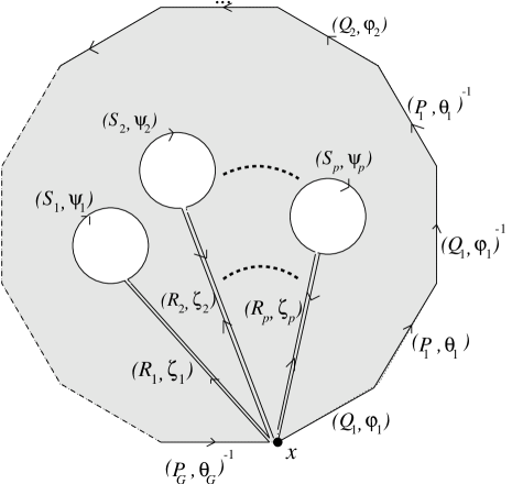
Figure 1: The lattice theory on a surface of genus $G$ with $p$ boundaries can be reduced to a single plaquette with suitably identified edges.

These results can easily be generalized to a surface of arbitrary genus and an arbitrary number of boundaries. In Fig. 1 a surface of genus $G$ with $p$ boundaries is represented as a single plaquette with suitably identified edges. The group elements of ${\cal G}_{N}$ associated to each link are also indicated in the figure. The partition function is then given by:

$$Z_{N}\left(\widehat{S_{1}\psi_{1}},\widehat{S_{2}\psi_{2}},....,\widehat{S_{p}\psi_{p}},{\cal A},G\right)=\sum_{P_{a},Q_{a},R_{A}}\int\prod_{i=1}^{N}\,\prod_{a=1}^{G}\frac{d\varphi_{a,i}d\theta_{a,i}}{4\pi^{2}}\prod_{A=1}^{p}\frac{d\zeta_{A,i}}{2\pi}$$

$$\delta(\Omega)\sum_{\{n_{i}\}}\left\{\sum_{i}\{{\rm i}n_{i}\omega_{i}-{\cal A}v(n)\}\right\}~{},$$ (36)

where the hats at the l.h.s. are to denote that $Z_{G}$ only depends on the conjugacy classes of $(S_{A},\psi_{A})$. $\Omega$ is the product of all permutations along the plaquette. Using the shorthand notation

$$V_{A}=R_{A}S_{A}R_{A}^{-1}~{},~{}~{}~{}~{}~{}~{}~{}~{}~{}~{}~{}W_{a}=Q_{a}P_{a}Q_{a}^{-1}P_{a}^{-1}$$ (37)

it can be written as

$$\Omega=V_{1}V_{2}...V_{p}W_{1}W_{2}.......W_{G}~{}.$$ (38)

The angles $\omega_{i}$ are the corresponding U$(1)^{N}$ invariant angles:

$$\omega = \sum_{A=1}^{p}(V_{1}V_{2}...V_{A-1}R_{A}\psi_{A}+V_{1}V_{2}...V_{A-1}\zeta_{A}-V_{1}V_{2}...V_{A}\zeta_{A})$$ (39)

$$+ \sum_{a=1}^{G}(V_{1}...V_{p}W_{1}...W_{a-1}\varphi_{a}-V_{1}...V_{p}W_{1}...W_{a-1}Q_{a}P_{a}Q_{a}^{-1}\varphi_{a}$$

$$+ V_{1}...V_{p}W_{1}...W_{a-1}Q_{a}\theta_{a}-V_{1}...V_{p}W_{1}...W_{a-1}W_{a}\theta_{a})~{}.$$

The integrations over $\zeta_{A,i}$, $\varphi_{a,i}$ and $\theta_{a,i}$ produce a set of delta functions that identify some (or all) of the integers $n_{i}$, namely:

$$\widehat{\delta(n)} = \prod_{i=1}^{N}\prod_{A=1}^{p}\delta\left(n_{i},n_{V_{1}V_{2}..V_{A-1}V_{A}V_{A-1}^{-1}...V_{2}^{-1}V_{1}^{-1}(i)}\right)$$

$$\times \prod_{i=1}^{N}\prod_{a=1}^{G}\delta\left(n_{i},n_{V_{1}...V_{p}W_{1}...W_{a-1}Q_{a}P_{a}Q_{a}^{-1}W_{a-1}^{-1}...W_{1}^{-1}V_{p}^{-1}...V_{1}^{-1}(i)}\right)$$

$$\times \prod_{i=1}^{N}\prod_{a=1}^{G}\delta\left(n_{i},n_{V_{1}...V_{p}W_{1}...W_{a-1}Q_{a}P_{a}Q_{a}^{-1}P_{a}^{-1}Q_{a}^{-1}W_{a-1}^{-1}...W_{1}^{-1}V_{p}^{-1}...V_{1}^{-1}(i)}\right)~{}.$$

The set of $\delta$-functions of Eq. (LABEL:deltas) are in one-to-one correspondence with the generators of the homotopy group of ${\cal M}$ with base point $X$. So all the integers $n_{i}$ with indices that can obtained from each other by acting with an element of the homotopy group are identified.

By taking into account the definitions (37) and (38) and the result (LABEL:deltas), the final expression for the partition function (36) is given by

$$Z_{N}\left(\widehat{S_{1}\psi_{1}},\widehat{S_{2}\psi_{2}},....,\widehat{S_{p}\psi_{p}},{\cal A},G\right)=\sum_{P_{a},Q_{a},R_{A}}\delta(\Omega)\sum_{\{n_{i}\}}\widehat{\delta(n)}$$

$$\times\exp\left\{\sum_{i}\left({\rm i}n_{i}\sum_{A=1}^{p}(V_{1}V_{2}...V_{A-1}R_{A}\psi_{A})_{i}-{\cal A}v(n_{i})\right)\right\}~{}.$$ (41)

In Eq. (41) the sum over $P_{a},Q_{a},R_{A}$ with the constraint given by $\delta(\Omega)$ counts the number of coverings with the prescribed conditions at the boundaries, while $\widehat{\delta(n)}$ ensures that each connected world-sheet contributes with a factor which is exactly the U$(1)$ kernel given in (25). It should be noticed that the r.h.s. of (41) depends only on the conjugacy classes of $(S_{A},\psi_{A})$, namely on the cycle decomposition of $S_{A}$ and, for each cycle $C$ of $S_{A}$, on the quantities $\psi_{A}^{C}=\sum_{i\in C}\psi_{A,i}$. This is a consequence of gauge invariance under ${\cal G}_{N}$ transformations but it can be seen explicitly from (41) by noticing that $S_{A}$ appears only in the expression $R_{A}S_{A}R_{A}^{-1}$ (with a sum over $R_{A}$), and that all $\psi_{A,i}$ with $i\in C$ are coupled to the same integer $n$ due to the effect of $\widehat{\delta(n)}$. Finally it should be remarked that the kernel (41) is completely consistent in the sense that it is reproduced by sewing two surfaces together according to the standard procedure, namely by identifying the conjugacy classes of the boundaries to be sewn and by integrating over the group.

5 Partition function on arbitrary genus

In order to write an explicit expression for the partition function (or kernel) given in (41), we have to use techniques developed by several authors [6, 16] that allow to write the number of coverings on a given surface in terms of the characters of $S_{N}$. In this section we will restrict the discussion to the case of surfaces without boundaries, while in the next section the general case of surfaces with boundaries will be discussed. We can proceed in four steps:

1. Write the partition function that describes the statistics of the coverings without branch points on a surface of genus $G$, that is

   $$Z^{(\rm cov)}(G,q)=\sum_{k=1}^{\infty}Z_{k}^{(\rm cov)}(G)q^{k}~{},$$ (42)

   where $Z_{k}^{(\rm cov)}(G)$ is the number of $k$-coverings. This partition function was studied in [6, 16] and it will be given below.

2. Write the partition function $F^{(\rm cov)}(G,q)$ that describes the statistics of connected coverings. This is obtained by taking the logarithm of $Z^{(\rm cov)}(G,q)$:

   $$F^{(\rm cov)}(G,q)=\log Z^{(\rm cov)}(G,q)=\sum_{k=1}^{\infty}F_{k}^{(\rm cov)}(G)q^{k}~{}.$$ (43)

3. Associate to each connected covering the U$(1)$ partition function (23):

   $$F({\cal A},G,q)=\sum_{k=1}^{\infty}F_{k}^{(\rm cov)}(G)\sum_{n=-\infty}^{+\infty}{\rm e}^{-k{\cal A}v(n)}q^{k}=\sum_{n=-\infty}^{+\infty}F^{(\rm cov)}(G,{\rm e}^{-{\cal A}v(n)}q)$$ (44)

4. The exponential of $F({\cal A},G,q)$ is then the generating function (i.e. grand-canonical partition function) for the partition functions given in (41) with no boundaries ($p=0$):

   $$Z({\cal A},G,q)={\rm e}^{F({\cal A},G,q)}=\sum_{N=1}^{\infty}Z_{N}({\cal A},G)q^{N}=\prod_{n=-\infty}^{+\infty}Z^{(\rm cov)}(G,{\rm e}^{-{\cal A}v(n)}q)~{}.$$ (45)

All we need to know, in order to write $Z({\cal A}G,q)$, is the explicit expression of $Z^{(\rm cov)}(G,q)$, that was given in [6, 16] as a sum over irreducible representations of $S_{N}$ as $N\rightarrow\infty$:

$$Z^{(\rm cov)}(G,q)=\sum_{\{h_{i}\}}\left[N^{|h|}\Lambda(h)\right]^{2G-2}q^{|h|}~{},$$ (46)

where

$$|h|=\sum_{i=1}^{N}h_{i}-\frac{1}{2}N(N-1)$$ (47)

and

$$\Lambda(h)=\frac{\prod_{i=1}^{N}h_{i}!}{\prod_{i<j}(h_{i}-h_{j})}~{}.$$ (48)

The integers $h_{i}$ are subjected to the constraint $h_{1}>h_{2}>.....>h_{N}\geq 0$ and are related to the lengths $m_{1},m_{2},...,m_{N}$ of the rows of the corresponding Young tableau by $h_{i}=N-i+m_{i}$. The quantity $|h|=\sum_{i}m_{i}$ is the number of boxes in the Young tableau.

The integer $N$ in Eq. (46) is just the order of the matrices in the complex matrix model introduced in Ref. [16], and whose solution is given by Eq. (46). No such quantity is present in the original problem of counting coverings, so there must be no dependence on $N$ at the end. The factor $N^{|h|(2G-2)}=N^{2g-2}$ just counts the genus $g$ of the world-sheet and it will be dropped in what follows. All the other quantities in (46) depend only on the Young tableau and not on the order $N$ of the symmetric group. However the limit $N\rightarrow\infty$ has to be taken in order to take into account Young tableaux with an arbitrarily large number of rows.

Figure 2: Ground state and lowest-lying excited states in the fermionic description of the representations of $S_{N}$, together with the corresponding Young tableaux.

In order to make this more explicit and also to simplify the expression of (46) we introduce a notation where each Young tableau is associated to an excited state of a gas of fermions whose energy levels are the relative integers (see [19] for an analogous notation in the case of U$(N)$). The ground state ($|h|=0$) and the lowest excited states are shown in Fig. 2; they are in one-to-one correspondence with the Young tableaux. The correspondence is as follows: let the infinite sequence of relative integers $h_{1}>h_{2}>h_{3}>.........$ represent the occupied levels and the complementary sequence $k_{1}<k_{2}<k_{3}<.......$ the empty levels. By definition $\{h_{i}\}\cup\{k_{j}\}={\bf Z}$ and $\{h_{i}\}\cap\{k_{j}\}=\emptyset$. The position of the origin is irrelevant, so the sequences $\{h_{i}\}$ and $\{k_{j}\}$ are defined modulo an integer shift. The length $m_{i}$ of the $i$-th row of the Young tableau is given by the number of empty levels below $h_{i}$:

$$m_{i}=\#k_{j}:\,k_{j}<h_{i}$$ (49)

and similarly the length $r_{j}$ of the $j$-th column by the number of the occupied levels above $k_{j}$:

$$r_{j}=\#h_{i}:\,k_{j}<h_{i}~{}.$$ (50)

The total number of boxes is the number of pairs $\{k_{j},h_{i}\}$ for which $h_{i}>k_{j}$:

$$|h|=\#\{k_{j},h_{i}\}:\,k_{j}<h_{i}~{}.$$ (51)

This coincides with the number of “moves” required to reach the excited state under consideration from the ground state, a move being defined as a jump of a fermion one level up to occupy an empty level. The Young tableaux with given $|h|$ label the irreducible representations of $S_{|h|}$, and the factor $\Lambda(h)$ given in Eq. (48) is related to the dimension $d_{\{h\}}$ of the corresponding representation by:

$$\Lambda(h)=\frac{|h|!}{d_{\{h\}}}~{}.$$ (52)

A simple calculation shows that $\Lambda(h)$ can be rewritten as $\prod_{\{h_{i}>k_{j}\}}(h_{i}-k_{j})$.The partition function of the coverings can then be written without any reference to $N$ as:

$$Z^{(\rm cov)}(G,q)=\sum_{h_{1}>h_{2}>....}\left[\prod_{\{h_{i}>k_{j}\}}(h_{i}-k_{j})\right]^{2G-2}q^{|h|}=\sum_{\{h\}}\left[\frac{d_{\{h\}}}{|h|!}\right]^{2-2G}q^{|h|}~{}.$$ (53)

The coefficients of the expansion of $Z^{(\rm cov)}(G,q)$ can be easily calculated from (53), and the first few of them are reproduced in the Appendix. The grand-canonical partition function $Z({\cal A},G,q)$ can be obtained in principle by inserting (53) into (45) and the first few coefficient of the expansion are also given in the Appendix. Except for $G=0$ and $G=1$ no compact expression for $Z^{(\rm cov)}(G,q)$ or $Z({\cal A},G,q)$ is available.

For $G=0$ we have $Z^{(\rm cov)}(G=0,q)={\rm e}^{q}$ and the U$(N)$ partition function is simply given by

$$Z_{N}({\cal A},G=0)=\left(\sum_{n=-\infty}^{\infty}{\rm e}^{-{\cal A}v(n)}\right)^{N}~{}.$$ (54)

This means that for the topology of the sphere our theory reduces to $N$ copies of the corresponding abelian theory.

As already discussed in [8], $Z^{(\rm cov)}(G,q)$ can be written for $G=1$ as an infinite product, and $Z({\cal A},G=1,q)$ is given by:

$$Z({\cal A},G=1,q)=\prod_{n=-\infty}^{\infty}\prod_{k=1}^{\infty}\frac{1}{1-q^{k}{\rm e}^{-k{\cal A}v(n)}}~{}.$$ (55)

6 Surfaces with boundaries

Consider a surface ${\cal M}_{G,p}$ of genus $G$ and with $p$ boundaries. As discussed in the previous section, the original U$(N)$ gauge theory is described by the $N$-coverings of ${\cal M}_{G,p}$ with a residual U$(1)$ gauge theory on each world-sheet. The states at the $A$-th boundary are then characterized by :

1. The conjugacy class of $P(\gamma_{A})$, where $\gamma_{A}$ is any closed path that can be deformed into the boundary (see Section 2). Each conjugacy class is given in terms of the length of the cycles of $P(\gamma_{A})$, namely of the set of integers $\{r_{l}^{(A)}\}$ with $\sum_{l=1}^{N}lr_{l}^{(A)}=N$.

2. The U$(1)$ holonomy associated to each boundary of any world-sheet, that is to each cycle of $P(\gamma_{A})$. The holonomy is given by an invariant angle $\theta_{l,\alpha}^{(A)}$, where the label $\alpha=1,2,...,r_{l}^{(A)}$ enumerates the cycles of the same length. Since the cycles of same length are indistinguishable, we expect the wave function to be symmetric in the corresponding angles.

Let us first consider the case where no U$(1)$ gauge theory is present, namely the pure theory of coverings. The grand-canonical partition function that describes the statistics of the coverings on a surface with $p$ boundaries and genus $G$ is defined by

$$Z^{(\rm cov)}(G,p,t_{l}^{(A)})=\sum_{\{r_{l}^{(A)}\}}Z^{(\rm cov)}(G,p,r_{l}^{(A)})\prod_{A=1}^{p}\prod_{l=1}^{\infty}\left[t_{l}^{(A)}\right]^{r_{l}^{(A)}}~{}.$$ (56)

Here $Z^{(\rm cov)}(G,p,r_{l}^{(A)})$ is the number of coverings with $r_{l}^{(A)}$ cycles of length $l$ on the $A$-th boundary. Its explicit form was given in [16] and with the notations of Section 5 it reads

$$Z^{(\rm cov)}(G,p,r_{l}^{(A)})=\sum_{\{h_{i}\}}\left[\Lambda(h)\right]^{2G-2+p}\prod_{A=1}^{p}\frac{\chi_{h}(r^{(A)}_{l})}{\prod_{l}l^{r^{(A)}_{l}}r^{(A)}_{l}!}~{},$$ (57)

where $\chi_{h}(r^{(A)}_{l})$ are the characters of $S_{|h|}$ if $r^{(A)}_{1}+2r^{(A)}_{2}+3r^{(A)}_{3}+.....=|h|$ and zero otherwise. It is important to notice that sewing two surfaces together reproduces the same grand-canonical partition function through the orthogonality properties of the characters, in exactly the same way as it happens in the Rusakov partition function of YM2.

The grand-canonical partition function for connected coverings is obtained as usual by

$$F^{(\rm cov)}(G,p,t_{l}^{(A)}) = \log Z^{(\rm cov)}(G,p,t_{l}^{(A)})$$ (58)

$$= \sum_{r_{l}^{(A)}}F^{(\rm cov)}(G,p,r_{l}^{(A)})\prod_{A=1}^{p}\prod_{l=1}^{\infty}\left[t_{l}^{(A)}\right]^{r_{l}^{(A)}}~{}.$$

The number of connected coverings $F^{(\rm cov)}(G,p,r_{l}^{(A)})$ can in principle be calculated from (58) and (56), although no closed expression is available.

Let us now introduce the U$(1)$ gauge theory. We are interested in the kernels $Z(G,p,r_{l}^{(A)},\theta^{(A)}_{l,\alpha})$, namely in the partition function with prescribed boundary conditions. It is convenient to introduce the kernels in momentum space of the angular variables $\theta^{(A)}_{l,\alpha}$, namely

$$Z\left({\cal A},G,p,r_{l}^{(A)},n^{(A)}_{l,\alpha}\right) = \int_{0}^{2\pi}\prod_{A,l,\alpha}d\theta^{(A)}_{l,\alpha}\exp\left\{\sum_{A,l,\alpha}{\rm i}n^{(A)}_{l,\alpha}\theta^{(A)}_{l,\alpha}\right\}$$ (59)

$$Z({\cal A},G,p,r_{l}^{(A)},\theta^{(A)}_{l,\alpha})~{}.$$

In momentum space the boundary conditions are now completely specified by giving $r_{l}^{(A)}$ and $n^{(A)}_{l,\alpha}$. However, since two cycles of the same length and momentum are indistinguishable, we can label the state at each boundary $i$ by the number $r^{(A)}_{n,l}$ of cycles of length $l$ and momentum $n$:

$$r^{(A)}_{n,l}=\sum_{l,\alpha}\delta_{n,n^{(A)}_{l,\alpha}}~{}.$$ (60)

So we shall write $Z\left({\cal A},G,p,r^{(A)}_{n,l}\right)$ instead of $Z\left({\cal A},G,p,r_{l}^{(A)},n^{(A)}_{l,\alpha}\right)$. The corresponding grand-canonical function can be written as

$$Z\left({\cal A},G,p,t^{(A)}_{n,l}\right)=\sum_{\{r^{(A)}_{n,l}\}}Z\left({\cal A},G,p,r^{(A)}_{n,l}\right)\prod_{A=1}^{p}\prod_{l=1}^{\infty}\prod_{n=-\infty}^{+\infty}\left[t_{n,l}^{(A)}\right]^{r^{(A)}_{n,l}}~{}.$$ (61)

As usual we also introduce the grand-canonical function that corresponds to the connected coverings:

$$F\left({\cal A},G,p,t^{(A)}_{n,l}\right)=\log Z\left({\cal A},G,p,t^{(A)}_{n,l}\right)~{}.$$ (62)

The structure of $F\left({\cal A},G,p,t^{(A)}_{n,l}\right)$ is determined by the following considerations. A U$(1)$ partition function, as in Eq. (23):

$$K_{{\rm U}(1)}(k{\cal A},\theta)=\sum_{n=-\infty}^{+\infty}{\rm e}^{-k{\cal A}v(n)+{\rm i}n\theta}$$ (63)

is associated to each connected part of the world-sheet. Here $k$ is the degree of the covering and $\theta$ is the sum over all the invariant U$(1)$ angles associated to the cycles of the world-sheet’s boundaries. It is clear then that, due to the angular integrations in Eq. (59), all cycles belonging to the same connected covering have the same momentum $n$ irrespective of the boundary on which they are situated. Moreover, the total length $|r|_{n}$ of the cycles with a given momentum $n$ is the same for all boundaries of ${\cal M}_{G,p}$:

$$\sum_{l}lr^{(A)}_{n,l}=|r|_{n}~{}.$$ (64)

In conclusion, each term of $F\left({\cal A},G,p,t^{(A)}_{n,l}\right)$ is characterized by a unique momentum $n$, is weighted by the factor ${\rm e}^{-|r_{n}|{\cal A}v(n)}$ coming from the U$(1)$ kernel and is proportional to the number $F^{(\rm cov)}\left(G,p,r^{(A)}_{n,l}\right)$ of connected coverings with cycles of given lengths:

$$F\left({\cal A},G,p,t^{(A)}_{n,l}\right)=\sum_{n=-\infty}^{+\infty}F^{(\rm cov)}\left(G,p,r^{(A)}_{n,l}\right)\prod_{A=1}^{p}\prod_{l=1}^{\infty}\left[t_{n,l}^{(A)}\right]^{r^{(A)}_{n,l}}{\rm e}^{-|r|_{n}{\cal A}v(n)}~{}.$$ (65)

The expression for the kernel $Z\left({\cal A},G,p,t^{(A)}_{n,l}\right)$ can be obtained by exponentiating both sides of Eq. (65) and it can be written as an infinite product:

$$Z\left({\cal A},G,p,t^{(A)}_{n,l}\right)=\prod_{n=-\infty}^{+\infty}Z^{(\rm cov)}\left(G,p,{\rm e}^{-l{\cal A}v(n)}t^{(A)}_{n,l}\right)$$ (66)

Each term in the infinite product in Eq. (66) is the grand-canonical partition function for the coverings defined in Eq. (56) with $t^{(A)}_{l}$ replaced by ${\rm e}^{-lv(n)}t^{(A)}_{n,l}$. This is the analogue of Eq. (45) for kernels with boundaries.

Starting from eq. (66) one can obtain the result, already known fron the lattice formulation os Section 4, that by sewing together two surfaces we obtain a kernel described again by Eq. (66) for the resulting surface. This follows from the fact that same property holds for the partition function of the coverings $Z^{(\rm cov)}\left(G,p,t^{(A)}_{l}\right)$. In fact when sewing two boundaries together the U$(1)$ invariant angles on the two sides have to be identified in pairs (for cycles of the same length!) and integrated over. This gives a delta function of the corresponding momenta, so that for each subspace of given momentum $n$ the sewing and cutting is unaffected by the other subspaces and its statistics coincides with the one of the pure covering theory.

7 Conclusions and further developments

The quantization of YM2 in the unitary gauge on an arbitrary Riemann surface has led us to consider a different model, a generalized YM2 theory whose effective theory, after integration over the non-Cartan component of the gauge fields, is described by a string with a U$(1)$ gauge group on the world-sheet. This theory coincides with a gauge theory on a lattice with gauge group ${\cal G}_{N}$, the semi-direct product of the symmetric group $S_{N}$ and U$(1)^{N}$. It may be surprising that the partition function on an arbitrary genus surface of our original U$(N)$ gauge theory can be calculated exactly within the gauge theory of a group ${\cal G}_{N}$ which is a subgroup of the original gauge group. However there are correlators of the original U$(N)$ gauge theory that cannot be calculated in the framework of the effective theory. Consider for instance correlators of Wilson loops, which depend on the non-Cartan components of the U$(N)$ gauge fields. If the Wilson loops are non intersecting, such components are irrelevant as the quadratic term in the off-diagonal action (13) depends at each space-time point on both space-time components of $\hat{A}_{a}^{ij}$. For intersecting Wilson loops instead this term produces an interaction between different sheets of the covering whose effect cannot be described in terms of the pure ${\cal G}_{N}$ theory. The situation is somewhat similar to the one in multi-matrix models, where the angular degrees of freedom can be integrated out in the calculation of the partition function and of certain correlators but are involved in a non trivial way in the most general correlators.

Besides its relation with YM2, the ${\cal G}_{N}$ gauge theory is interesting by itself, and it can generalized in two different directions that we shall briefly mention here, while leaving the details for a future publication [21].

The first type of extension is the one already considered in [16] for the theory of coverings. It consists in allowing coverings with branch points, namely in allowing the strings to split and join. In the framework of Matrix string theory this was discussed in  [20, 17]. A branch point can be described as a boundary where all the U$(1)$ invariant angles are set to zero. In this case, if the permutation associated to the boundary is trivial this just becomes an ordinary point, otherwise it becomes a point where a more or less complicated interaction amongst the sheets of the covering occurs. The simplest case consists in a single string splitting into two strings or vice-versa, and it is described by a permutation with only one non trivial cycle of order $2$. ¿From this point of view the results of Section 6 are all we need to introduce branch points in our theory. However we want to consider, as in [16], the limit where a continuum distribution of branch points is introduced. For the theory of pure coverings, that is for the gauge theory of $S_{N}$, this corresponds to replacing the plaquette action, which for the unbranched theory of coverings is just a delta function, with a sum over irreducible representations of $S_{N}$:

$$\delta(P)=\sum_{R}d_{R}\chi_{R}(P)\rightarrow\sum_{R}d_{R}\chi_{R}(P){\rm e}^{-C_{R}}~{}.$$ (67)

Here $P$ is the permutation associated to the plaquette and $C_{R}$ is any quantity that depends only on the representation $R$ and that contains all the information about the couplings of the different types of branch points (see [16] for details).

In our ${\cal G}_{N}$ gauge theory the introduction of a continuum of branch points will amount to replacing the plaquette action (26) with a generic expansion in the characters of the irreducible representations of ${\cal G}_{N}$. The weight of each representation should contain the area ${\cal A}$ of the plaquette at the exponent, to insure good gluing properties as in (34), and will depend both on the potential $v(n)$ that appears in the original action and on the couplings of the different types of branch points encoded in $C_{R}$. These couplings are new free parameters of the theory which are not present in the original Lagrangian. As they describe interactions amongst different sheets, they would presumably correspond to singular terms in the U$(1)^{N}$ gauge theory obtained after fixing the unitary gauge, possibly of the same type as the ones that have been eliminated by the redefinition of the potential. A different type of extension is obtained by considering a more general gauge group ${\cal G}_{L,M}$, defined as the semi-direct product of $S_{L}$ and U$(M)^{L}$. The product law in ${\cal G}_{L,M}$ is explicitly given by

$$(P,g_{i})(Q,h_{i})=(PQ,g_{i}h_{P^{-1}(i)})~{},$$ (68)

where $P$ and $Q$ are elements of $S_{L}$, $g_{i}$ and $h_{i}$ ($i=1,2,...,L$) are elements of U$(M)$ and the products at the r.h.s. of (68) are accordingly group products in $S_{L}$ and U$(M)$. The gauge theory based on this group describes a theory of coverings (with possibility of introducing branch points as above) with a U$(M)$ on each world-sheet. This theory would include both the standard YM2 and the ${\cal G}_{N}$ theory described in this paper as particular cases. Its plaquette action (without branch points) can be easily constructed by following the same line of reasoning used to obtain Eq. (26), and it reads

$$K\left((P,g_{i}),{\cal A}\right)=\delta(P)\prod_{i=1}^{L}\sum_{R^{(i)}}d_{R^{(i)}}\chi_{R^{(i)}}(g_{i})e^{-{\cal A}C_{R^{(i)}}}~{},$$ (69)

where $R^{(i)}$ are the representations of the $i$-th group U$(M)$ and are labeled by a set of $M$ integers $\{n^{(i)}\}$. The whole theory can now be constructed by sewing plaquettes together and it is essentially obtained by replacing in the formulas of Section 4 the integer momentum $n$ with the representations of U$(M)$ and the plane wave function $e^{{\rm i}n\theta}$ with the characters $\chi_{R^{(i)}}(g)$. By allowing branch points in the string theories based on ${\cal G}_{L,M}$ we can construct a large class of string theories, that range from the pure U$(M)$ theory (standard YM2 theory) at one end to the pure theory of coverings at the other end. The well known result of Gross and Taylor [6], namely that in the large $N$ YM2 is equivalent to a theory of coverings with a set of allowed interactions, suggests that the same kind of dual description may be possible also for the more general theories we have discussed.

Acknowledgments

We thank M. Caselle for many useful discussions. One of us (A. D.) also thanks G. Semenoff for discussions.

Appendix

In this Appendix we display explicitly the coefficients of the grand-canonical partition functions for the coverings and the generalized Yang-Mills theory up to order $q^{5}$.

Let us consider first $Z^{(\rm cov)}(G,q)$ defined in Eq. (42). Each coefficient $Z^{(\rm cov)}_{k}(G)$ is the number of inequivalent unbranched $k$-coverings of a genus $G$ surface without boundaries. Two coverings are said to be inequivalent if they cannot be obtained from each other by simple relabeling of the sheets; therefore the total number of $k$-coverings is $k!Z^{(\rm cov)}_{k}(G)$.

Naming $\chi=2-2G$ the Euler characteristic of the surface ${\cal M}$, from Eq. (53) we obtain:

$$Z^{(\rm cov)}_{0}(G) = 1~{},$$

$$Z^{(\rm cov)}_{1}(G) = 1~{},$$

$$Z^{(\rm cov)}_{2}(G) = 2\cdot 2^{-\chi}~{},$$

$$Z^{(\rm cov)}_{3}(G) = 2\cdot 6^{-\chi}+3^{-\chi}~{},$$

$$Z^{(\rm cov)}_{4}(G) = 2\cdot 24^{-\chi}+12^{-\chi}+2\cdot 8^{-\chi}~{},$$

$$Z^{(\rm cov)}_{5}(G) = 2\cdot 120^{-\chi}+2\cdot 30^{-\chi}+2\cdot 24^{-\chi}+20^{-\chi}~{}.$$ (70)

The number of inequivalent connected coverings are given by the coefficients in the power expansion in $q$ of $\log Z^{(\rm cov)}(G,q)$. Here we give the list up to $k=5$:

$$F^{(\rm cov)}_{1}(G) = 1~{},$$

$$F^{(\rm cov)}_{2}(G) = 2\cdot 2^{-\chi}-1/2~{},$$

$$F^{(\rm cov)}_{3}(G) = 2\cdot 6^{-\chi}+3^{-\chi}-2\cdot 2^{-\chi}+1/3~{},$$

$$F^{(\rm cov)}_{4}(G) = 2\cdot 24^{-\chi}+12^{-\chi}+2\cdot 8^{-\chi}$$

$$- 2\cdot 6^{-\chi}-3^{-\chi}+2\cdot 2^{-\chi}-2\cdot 4^{-\chi}-1/4~{},$$

$$F^{(\rm cov)}_{5}(G) = 2\cdot 120^{-\chi}+2\cdot 30^{-\chi}+20^{-\chi}-5\cdot 12^{-\chi}$$ (71)

$$- 2\cdot 8^{-\chi}+4\cdot 4^{-\chi}+3^{-\chi}-2\cdot 2^{-\chi}+1/5~{}.$$

By inserting Eqs. (70) and (71) into Eqs. (44) and (45) we can write the first few terms in the expansion of $Z(G,{\cal A},q)$, namely the partition functions $Z_{N}({\cal A},G)$ for $N$ up to 5:

$$Z_{0}({\cal A},G) = 1~{},$$

$$Z_{1}({\cal A},G) = z({\cal A})~{},$$

$$Z_{2}({\cal A},G) = \left(2\cdot 2^{-\chi}-\frac{1}{2}\right)z(2{\cal A})+\frac{1}{2}z^{2}({\cal A})~{},$$

$$Z_{3}({\cal A},G) = \left(2\cdot 6^{-\chi}+3^{-\chi}-2\cdot 2^{-\chi}+\frac{1}{3}\right)z(3{\cal A})$$

$$+ \left(2\cdot 2^{-\chi}-\frac{1}{2}\right)z({\cal A})z(2{\cal A})+\frac{1}{6}z^{3}({\cal A})~{},$$

$$Z_{4}({\cal A},G) = \Bigl{(}2\cdot 24^{-\chi}+12^{-\chi}+2\cdot 8^{-\chi}-2\cdot 6^{-\chi}\Bigr{.}$$

$$- \left.3^{-\chi}+2\cdot 2^{-\chi}-2\cdot 4^{-\chi}-\frac{1}{4}\right)z(4{\cal A})$$

$$+ \frac{1}{2}\left(4\cdot 4^{-\chi}-2\cdot 2^{-\chi}+\frac{1}{4}\right)z^{2}(2{\cal A})$$

$$+ \left(2\cdot 6^{-\chi}+3^{-\chi}-2\cdot 2^{-\chi}+\frac{1}{3}\right)z({\cal A})z(3{\cal A})$$

$$+ \frac{1}{2}\left(2\cdot 2^{-\chi}-\frac{1}{2}\right)z(2{\cal A})z^{2}({\cal A})+\frac{1}{24}z^{4}({\cal A})~{},$$

$$Z_{5}({\cal A},G) = \Bigl{(}2\cdot 120^{-\chi}+2\cdot 30^{-\chi}+20^{-\chi}-5\cdot 12^{-\chi}\Bigr{.}$$ (72)

$$- \left.2\cdot 8^{-\chi}+4\cdot 4^{-\chi}+3^{-\chi}-2\cdot 2^{-\chi}+\frac{1}{5}\right)z(5{\cal A})$$

$$+ \left(2\cdot 24^{-\chi}+12^{-\chi}+2\cdot 8^{-\chi}-2\cdot 6^{-\chi}\right.$$

$$- \left.3^{-\chi}+2\cdot 2^{-\chi}-2\cdot 4^{-\chi}-\frac{1}{4}\right)z(4{\cal A})z({\cal A})$$

$$+ \left(4\cdot 12^{-\chi}+6^{-\chi}-4\cdot 4^{-\chi}-\frac{1}{2}\cdot 3^{-\chi}\right.$$

$$+ \left.\frac{5}{3}\cdot 2^{-\chi}-\frac{1}{6}\right)z(2{\cal A})z(3{\cal A})$$

$$+ \frac{1}{2}\left(2\cdot 6^{-\chi}+3^{-\chi}-2\cdot 2^{-\chi}+\frac{1}{3}\right)z^{2}({\cal A})z(3{\cal A})$$

$$+ \frac{1}{2}\left(4\cdot 4^{-\chi}-2\cdot 2^{-\chi}+\frac{1}{4}\right)z({\cal A})z^{2}(2{\cal A})$$

$$+ \frac{1}{6}\left(2\cdot 2^{-\chi}-\frac{1}{2}\right)z^{3}({\cal A})z(2{\cal A})+\frac{1}{120}z^{5}({\cal A})~{},$$

where $z({\cal A})$ is a shorthand for $Z_{{\rm U}(1)}({\cal A})$, namely for the (generalized) U$(1)$ partition function on a surface of area ${\cal A}$:

$$z({\cal A})=\sum_{n}e^{-v(n){\cal A}}~{}.$$ (73)

References

- [1] A.A. Migdal, Sov. Phys. JETP 42 (1975) 413.
- [2] B. Ye. Rusakov, Mod. Phys. Lett. A5 (1990) 693.
- [3] E. Witten, Comm. Math. Phys. 141 (1991) 153.
- [4] E. Witten, J. Geom. Phys. 9 (1992) 303 hep-th/9204083.
- [5] M. Blau and G. Thompson, Int. J. Mod. Phys. A7 (1992) 3781
- [6] D.J. Gross, Nucl. Phys. B400 (1993) 161; D. Gross and W. Taylor, Nucl. Phys. B400 (1993) 181 and Nucl. Phys. B403 (1993) 395.
- [7] M. Billó, M. Caselle, A. D’Adda and P. Provero, Nucl.Phys. B543 (1999) 141.
- [8] M. Billó, M. Caselle, A. D’Adda and P. Provero, 2D Yang-Mills Theory as a Matrix String Theory, Proceedings Corfú Conference, ed.s Ceresole et al., Springer LNP 525, 1998, hep-th/9901053.
-
[9]
L. Motl, Proposals on nonperturbative superstring
interactions,
hep-th/9701025. - [10] R. Dijkgraaf, E. Verlinde and H. Verlinde, Nucl. Phys. B500 (1997) 43.
- [11] M. Blau and G. Thompson,“Lectures on Gauge Theories - Topological Aspects and Path Integral Techniques”, Proc. 1993 Summer School in High Energy Physics and Cosmology, ed.s E. Gava et al. (Trieste 1993), World Scientific,1994, hep-th/9310144
-
[12]
I.K. Kostov and P. Vanhove,
Phys. Lett. B444 (1998) 196,
hep-th/9809130. - [13] G. Grignani and G.W. Semenoff, hep-th/9903246.
- [14] M.R. Douglas, K. Li and M. Staudacher, Nucl. Phys. B420 (1994) 118.
- [15] O. Ganor, J. Sonnenschein and S. Yankielowicz, Nucl. Phys. B434 (1995) 139.
- [16] I. K. Kostov and M. Staudacher, Phys.Lett. B394 (1997) 75; I. K. Kostov, M. Staudacher and T. Wynter, Commun. Math. Phys. 191 (1998) 283.
- [17] G. Bonelli, L. Bonora and F. Nesti, Phys. Lett. B435 (1998) 303; G. Bonelli, L. Bonora and F. Nesti, Nucl. Phys. B538 (1999) 100; G. Bonelli, L. Bonora, F. Nesti and A. Tomasiello, Nucl. Phys. B554 (1999) 103.
- [18] M. Caselle, A. D’Adda and L. Magnea, Phys. Lett. B192 (1987) 406; M. Caselle, A. D’Adda and L. Magnea, Phys. Lett. B192 (1987) 411.
- [19] M.R. Douglas, Conformal field theory techniques in large N Yang-Mills theory, hep-th/9311130.
- [20] S.B. Giddings, F. Hacquebord and H. Verlinde, Nucl. Phys. B537 (1999) 260, hep-th/9804121.
- [21] M. Billó, A. D’Adda and P. Provero, in preparation