Non-Abelian Stokes Theorem and Quark Confinement in SU(N) Yang-Mills Gauge Theory

1 Introduction

Gell-Mann and Zweig [1] predicted in the mid-1960s that all hadrons (i.e., baryons and mesons) are composed of the fundamental constituents having fractional charges, $\pm{1\over 3}e$ or $\mp{2\over 3}e$, with $e$ being the elementary charge. Now, the fundamental constituent is called the quark and the proposed theory is called the quark model. The predictions of this model are consistent with the results of experiments performed over the past thirty years. The strong interaction among quarks and anti-quarks is mediated by the gluon, which is described by the quantized Yang-Mills gauge field theory. [2] The present fundamental theory describing the quark and the gluon is provided by quantum chromodynamics (QCD), which is a non-Abelian gauge theory with the gauge group $G=SU(3)$ corresponding to three colors. However, neither an isolated quark nor an isolated anti-quark has ever been observed experimentally. In the present understanding, they are believed to be confined in hadrons. This is the hypothesis of quark confinement. Quark confinement could be explained theoretically within the framework of QCD, although no one has achieved a rigorous proof of quark confinement. This is one of the most important problems to be solved in theoretical physics.

QCD has a remarkable property, called asymptotic freedom, which was discovered by Gross, Wilczek and Politzer and independently by ’t Hooft. [3] Asymptotic freedom does not appear in the most successful quantized field theory, quantum electrodynamics (QED). As is well known, QED is the Abelian gauge theory for the electron and the photon in which the electromagnetic interaction is described by the quantized Maxwell gauge field theory with the gauge group $G=U(1)$. Asymptotic freedom is a consequence of gluon self-interactions. Therefore, this is a very characteristic feature of non-Abelian gauge theory.

The purpose of this article is to demonstrate quark confinement within QCD based on the Wilson criterion for quark confinement, [4] i.e., the area law of the Wilson loop. The Wilson loop is a gauge invariant quantity and hence the Wilson criterion is also gauge invariant. The formulation of lattice gauge theory proposed by Wilson [4] is manifestly gauge invariant and does not need the gauge fixing. It is easy to show that the strong coupling expansion in lattice gauge theory leads to the area law of the Wilson loop. However, this result has not yet been continued to the weak coupling region, where the string tension is expected to obey the scaling law suggested from the result of the renormalization group based on loop calculations. The first indication of the area law of the Wilson loop for arbitrary coupling constant was found in a study based on numerical simulations within the lattice gauge theory by Creutz [5] for $G=SU(2)$ and $SU(3)$. Although the numerical evidence of quark confinement was indeed a great progress toward a complete understanding of quark confinement, the analytical proof is still lacking.

This work was initiated to justify the dual superconductor picture of the QCD vacuum proposed in the mid-1970s [6] within the framework of continuum quantum field theory. For dual superconductivity to occur, magnetic monopoles must be condensed, just as ordinary superconductivity requires condensation of Cooper pairs. In fact, the importance and the validity of taking into account magnetic monopoles in quark confinement has been demonstrated, at least for simplified four-dimensional and lower-dimensional models, especially, by Polyakov, [7] and recently for the four-dimensional Yang-Mills theory and QCD with extended supersymmetries by Seiberg and Witten. [8] In this scenario, quark confinement is realized due to condensation of magnetic monopoles. Recent developments in numerical simulations on the lattice [9] confirm the existence of dual superconductivity in QCD, at least, under a specific gauge fixing called the Abelian gauge.[10]

This article gives a detailed exposition of the results on quark confinement that were announced in a previous article [11] for $G=SU(3)$ together with new results for $G=SU(N)$ with arbitrary $N$. They are extensions of the analyses of the Yang-Mills theory in the maximal Abelian (MA) gauge given in a series of articles, [12, 13, 14, 15, 16, 17] where the case of $SU(2)$ was explicitly worked out. In this process, we have found that the extension from $SU(2)$ to $SU(3)$ is non-trivial, but the extension from $SU(3)$ to $SU(N)$, $N>3$, is rather straightforward. New features come out when we begin to analyze the $SU(N)$ case with $N\geq 3$. It seems that they have been overlooked to this time in the conventional approach based on the maximal Abelian gauge.

The MA gauge is a partial gauge fixing from the original non-Abelian gauge group $G$ to its subgroup $H$ [10] in which the gauge degrees of freedom of the coset $G/H$ are fixed. Even after the MA gauge, there is a residual gauge group $H$ which is taken to be the maximal torus subgroup $H=U(1)^{N-1}$. After the MA gauge, the magnetic monopole is expected to appear, since the Homotopy group $\pi_{2}(G/H)$ is non-trivial, i.e.,

$$\pi_{2}(SU(N)/U(1)^{N-1})=\pi_{1}(U(1)^{N-1})={\bf Z}^{N-1}.$$ (1.1)

This implies that the breaking of gauge group $G\rightarrow H$ by partial gauge fixing leads to ($N-1$) species of magnetic monopoles. However, we do not necessarily need to consider the maximal breaking $SU(N)\rightarrow U(1)^{N-1}$, although the maximal torus group is desirable as a gauge group of the low-energy effective Abelian gauge theory.[12] Actually, even if we restrict $H$ to a continuous subgroup of $G$, there are other possibilities for choosing $H$, e.g., we can choose a subgroup $\tilde{H}$ such that

$$G\supset\tilde{H}\supset H:=U(1)^{N-1}.$$ (1.2)

The possible number of cases for choosing $\tilde{H}$ increases as $N$ increases. We have found [11] that the group $\tilde{H}$ may depend on the representation to which the quark belongs when $N\geq 3$ and that it suffices to take $\tilde{H}=U(N-1)$ for the fundamental quark to be confined in the sense of the area law of the Wilson loop under the partial gauge fixing. Here $\tilde{H}$ is equal to the maximal stability group specified by the highest-weight state of the representation of the quark in the Wilson loop. This is a new feature which does not show up in the $SU(2)$ case. Nevertheless, this does not mean that the choice of the maximal torus does not lead to quark confinement. In fact, even if we choose the maximal torus, the area law can be derived. This is because the coset $G/\tilde{H}$ is contained in $G/H$, i.e., $G/\tilde{H}\subset G/H$, so that the Wilson loop does not feel the whole of $G/H$, but only feels the components of $G/\tilde{H}$ that are contained in $G/H$. In other words, the variables belonging to $G/H-G/\tilde{H}$ are irrelevant for the expectation value of the Wilson loop, as can be seen from the non-Abelian Stokes theorem (NAST) that was presented in Ref.? and is derived in this article. Therefore, a single kind of magnetic monopole is sufficient for confining a fundamental quark, since

$$\pi_{2}(SU(N)/U(N-1))=\pi_{1}(U(1))={\bf Z}.$$ (1.3)

Our results show that two partial gauge fixings $SU(3)\rightarrow U(2)$ and $SU(3)\rightarrow U(1)\times U(1)$ lead to the same result for confinement as far as the fundamental quarks are concerned.

The NAST plays the crucial role in this article. The NAST has a number of versions which have been derived by many authors.[20] The version of NAST derived in this article is based on the idea of Dyakonov and Petrov,[21] who derived an $SU(2)$ version and suggested a method of generalization. We derive a version of NAST based on the coherent state representation [22] on the flag space, [23, 24] not on the method suggested by them. The coherent state representation is used in a different fashion to derive an $SU(2)$ version of the NAST in Ref.?, but the extension to $SU(N)$, $N\geq 3$, was a non-trivial issue which prevented us from presenting immediate publication of general $SU(N)$ results. The NAST is not only mathematically (or technically) important but also physically interesting as we now discuss.

First, the NAST enables us to write the non-Abelian Wilson loop,

$$W^{C}[{\cal A}]:={1\over{\cal N}}{\rm tr}\left[{\cal P}\exp\left(ig\oint_{C}{\cal A}\right)\right],$$ (1.4)

in terms of the Abelian-field strength (curvature two-form) $f=da$ with the Abelian gauge potential (connection one-form) $a$:

$$W^{C}[{\cal A}]=\int[d\mu(V)]_{C}\exp\left(ig\oint_{C}a\right)=\int[d\mu(V)]_{C}\exp\left(ig\int_{S}f\right).$$ (1.5)

Combining this fact with the Abelian-projected effective gauge theory (APEGT) derived by one of the authors,[12] we can explain the Abelian dominance [25, 26] in the Wilson loop. The APEGT is an Abelian gauge theory obtained by integrating out the massive degrees of freedom, i.e., the off-diagonal gluon gauge field $A_{\mu}^{a}$ with mass $m_{A}$. Hence, the APEGT can be written in terms of the diagonal massless gauge field $a_{\mu}^{i}$ and the anti-symmetric (Abelian) tensor field $B_{\mu\nu}^{i}$ together with the ghost and anti-ghost fields $C^{a}$ and $\bar{C}^{a}$, where the index $i$ denotes the diagonal components and $a$ the off-diagonal ones. Therefore the APEGT is regarded as a low-energy effective theory (LEET) which is valid in the long-distance (or low-energy) region $R>m_{A}^{-1}$. The Abelian gauge field $b_{\mu}^{i}$ obtained after the Hodge decomposition of $B_{\mu\nu}^{i}$ can be identified with the Abelian gauge field dual to $a_{\mu}^{i}$. In fact, we can obtain the theory with an action $S[b]$ written in terms of $b_{\mu}^{i}$ alone by integrating out all the fields other than $b_{\mu}^{i}$ in APEGT, and the theory can be rewritten into the dual Ginzburg-Landau theory, i.e., the dual Abelian Higgs theory, provided that magnetic monopole condensation occurs, i.e., $\langle k_{\mu}k_{\mu}\rangle\not=0$. In the dual Ginzburg-Landau theory, the coupling constant $g$ in the original theory is replaced by the inverse coupling constant $1/g$ which is proportional to the magnetic charge. Therefore, the dual theory can be identified with the magnetic theory. On the other hand, the theory with an action $S[a]$ written in terms of $a^{i}$ alone is an Abelian gauge theory, but the scale dependence of the coupling constant $g(\mu)$ is the same as that in the original Yang-Mills theory. Thus the low-energy effective Abelian gauge theory exhibits asymptotic freedom reproducing the original renormalization-group beta function $\beta(g)$. This is a manifestation of an approximate weak-strong or electro-magnetic duality between two low-energy effective theories described by $S[a]$ and $S[b]$.

Next, the NAST is able to separate the piece $\omega$ which corresponds to the magnetic monopole in the Abelian field $a=C+\omega$. Indeed, we can write the $SU(N)$ version of the ’t Hooft-Polyakov tensor describing the magnetic monopole.[27] Hence we can separate the contribution of the magnetic monopole in the area law of the Wilson loop and explain the magnetic monopole dominance in quark confinement. In fact, our derivation of the area law estimates only the monopole contribution, $\mathchar 28938\relax_{K}=d\omega$. Moreover, the NAST tells us that the essential ingredient in the area law lies in the geometric phase, which is concerned with the holonomy group of $U(N-1)$. Thus we see that quark confinement is intimately related to the geometry of Yang-Mills gauge theory, in sharp contrast with the conventional wisdom.

We present two methods to derive the area law of the Wilson loop by making use of the NAST. The first method is to use the APEGT for estimating the diagonal Wilson loop; for a sufficiently large Wilson loop ($|C|\gg m_{A}^{-1}$), the expectation value of the non-Abelian Wilson loop in Yang-Mills theory is reduced to that of the Abelian Wilson loop in APEGT:

$${\hbox{$\left\langle\vbox to0.0pt{}\right.\n@space$}}W^{C}[{\cal A}]{\hbox{$\left\rangle\vbox to0.0pt{}\right.\n@space$}}_{YM}={\hbox{$\left\langle\vbox to0.0pt{}\right.\n@space$}}\exp\left(ig\oint_{C}a\right){\hbox{$\left\rangle\vbox to0.0pt{}\right.\n@space$}}_{YM}\rightarrow{\hbox{$\left\langle\vbox to0.0pt{}\right.\n@space$}}\exp\left(ig\oint_{C}a\right){\hbox{$\left\rangle\vbox to0.0pt{}\right.\n@space$}}_{APEGT}.$$ (1.6)

Then we can apply the result of Ref.?, confinement in the Abelian gauge theory, to show quark confinement in Yang-Mills theory.

The second method is to treat the non-Abelian gauge theory directly, without going through the effective Abelian gauge theory, based on the novel reformulation of Yang-Mills theory in the MA gauge which was proposed by one of the authors.[13] The novel reformulation regards the Yang-Mills theory as the perturbative deformation of a topological quantum field theory (TQFT). An advantage of this reformulation in the MA gauge is that the derivation of the area law of the non-Abelian Wilson loop in the four-dimensional $SU(N)$ Yang-Mills theory is reduced to that of the diagonal (Abelian) Wilson loop in the two-dimensional coset ($G/H$) non-linear sigma (NLS) model, at least when the Wilson loop is planar. Therefore the four-dimensional problem is reduced to a two-dimensional problem. This dimensional reduction is a remarkable feature of the modified MA gauge caused by hidden supersymmetry. The Yang-Mills coupling constant $g$ of the four-dimensional Yang-Mills theory is mapped into the coupling constant in the two-dimensional NLS model. Hence the coupling constant is expected to run in the same way as in the original Yang-Mills theory, since the perturbative deformation part provides the necessary running, as is well known from the loop calculation. For the fundamental quark, we are allowed to restrict the flag space $F_{N-1}:=SU(N)/U(1)^{N-1}$ to the complex projective space $CP^{N-1}:=SU(N)/U(N-1)$. This greatly simplifies the actual treatment.

Another advantage of this reduction is that the magnetic monopole contribution to the Wilson loop in the four-dimensional Yang-Mills theory in the MA gauge is equal to the instanton contribution in the corresponding two-dimensional NLS model. Indeed, the diagonal Wilson loop can be written as the area integral of the instanton density $\mathchar 28938\relax_{K}$ over the area $S$ bounded by the loop $C$. This correspondence may shed more light on the strong correlation between magnetic monopoles and instantons observed in the Monte Carlo simulations, since the two-dimensional instanton is identified as a subclass of the four-dimensional Yang-Mills instanton (see e.g. Ref.?).

In this article the expectation value of the Wilson loop is estimated by combining the instanton calculus and the large $N$ expansion. (See Refs.?, ?, ?, ? for reviews of the large $N$ expansion.) We focus on the $CP^{N-1}$ model corresponding to the fundamental quark. First, the instanton calculus is performed within the dilute gas approximation. It is shown that the calculation in the $SU(N)$ case reduces to that in the $SU(2)$ case. It is well known that the large $N$ expansion is a non-perturbative technique which can be systematically improved. We derive the area law to leading order in the large $N$ expansion, namely, in the region of large $N$ and weak coupling $g$. We hope that our derivation of quark confinement based on the dimensional reduction and the large $N$ expansion may shed more light on the relationship between QCD and string theory, as first suggested by ’t Hooft.[32]

This article is organized as follows. In the first half, we give a derivation of the NAST and discuss its implications. Sections 2 and 3 are preparations for $\S$ 4. In $\S$ 2 we review the construct of the coherent state on the flag space for the general compact semi-simple group $G$. In $\S$ 3, we present the explicit form of the coherent state on the flag space for $G=SU(N)$. We define the maximal stability group $\tilde{H}$, which is very important in the following discussion. In $\S$ 4, making use of the results of $\S\S$ 2 and 3, we derive a new version of the non-Abelian Stokes theorem for $G=SU(N)$. Although we discuss only the case of $SU(N)$ explicitly, it is straightforward to extend this theorem to an arbitrary compact semi-simple group $G$. This version of the non-Abelian Stokes theorem is very interesting not only from the mathematical but also from the physical point of view, since the non-Abelian Wilson loop is expressed as the surface integral of the two-form (i.e., the generalized ’t Hooft-Polyakov tensor), which leads to the magnetic monopole. This fact is intimately related with the Abelian and magnetic monopole dominance in quark confinement, as discussed in subsequent sections.

In the second half, we derive the area law of the Wilson loop. In $\S$ 5 we discuss the magnetic monopole in $SU(N)$ Yang-Mills theory. In order to specify the type of possible magnetic monopoles, it turns out that the maximal stability group is more important than the maximal torus group $H$. In $\S$ 6 Abelian dominance in the Wilson loop is shown in the $SU(N)$ Yang-Mills theory in the maximal Abelian gauge based on the Abelian-projected effective gauge theory and the non-Abelian Stokes theorem. In $\S$ 7 we briefly review a novel reformulation of the Yang-Mills theory which has been proposed by one of the authors [13] to derive quark confinement. This reformulation is called the (perturbative) deformation of the topological quantum field theory. We apply this reformulation to derive the area law of the Wilson loop in $SU(N)$ Yang-Mills theory in $\S\S$ 8 and 9. In $\S$ 9 we show within this reformulation that the area law of the Abelian Wilson loop in the two-dimensional nonlinear sigma model for the flag space $G/\tilde{H}$ is sufficient to derive the area law of the four-dimensional Yang-Mills theory in the maximal Abelian gauge. At the same time, this derivation leads to the magnetic monopole dominance in the area law. In $\S$ 8 we demonstrate the area law of the Wilson loop in the nonlinear sigma model in an approach based on naive instanton calculus. For the fundamental quark, we have only to deal with the $CP^{N-1}$ model. In $\S$ 9 we derive the area law based on the large $N$ expansion. These results imply the area law of the non-Abelian Wilson loop in the four-dimensional $SU(N)$ Yang-Mills theory. The final section contains the conclusion of this article.

In Appendix A, we give derivations of the inner product of the coherent states and the invariant measure on the flag space, which are presented in $\S$ 3. In Appendix B we explain the method of obtaining $CP^{1}$ and $CP^{2}$ by gluing the complex planes. In Appendix C, we explain two ways to characterize the element of the flag space and the manner of formulating the NLS model using these parameterizations. In Appendix D we summarize the large $N$ expansion of $CP^{N-1}$. In Appendix E supplementary material on the $1/N$ expansion is presented.

2 Coherent state and maximal stability group

First, we construct the coherent state $|\xi,\mathchar 28931\relax\rangle$ corresponding to the coset representatives $\xi\in G/\tilde{H}$. We follow the method of Feng, Gilmore and Zhang.[22] For inputs, we prepare the following:

1. the gauge group $G$ and the Lie algebra ${\cal G}$ of $G$ with the generators $\{T^{A}\}$, which obey the commutation relations

   $$[T^{A},T^{B}]=if^{AB}{}_{C}T^{C},$$ (2.1)

   where the $f^{AB}{}_{C}$ are the structure constants of the Lie algebra. If the Lie algebra is semi-simple, it is more convenient to rewrite the Lie algebra in terms of the Cartan basis $\{H_{i},E_{\alpha},E_{-\alpha}\}$. There are two types of basic operators in the Cartan basis, $H_{i}$ and $E_{\alpha}$. The operators $H_{i}$ may be taken as diagonal, while $E_{\alpha}$ are the off-diagonal shift operators. They obey the commutation relations

   $$[H_{i},H_{j}] = 0,$$ (2.2)

   $$[H_{i},E_{\alpha}] = \alpha_{i}E_{\alpha},$$ (2.3)

   $$[E_{\alpha},E_{-\alpha}] = \alpha^{i}H_{i},$$ (2.4)

   $$[E_{\alpha},E_{\beta}] = \cases{N_{\alpha;\beta}E_{\alpha+\beta},&($\alpha+\beta\in R$)\cr 0,&($\alpha+\beta\not\in R,\alpha+\beta\not=0$)}$$ (2.5)

   where $R$ is the root system, i.e., a set of root vectors $\{\alpha_{1},\cdots,\alpha_{r}\}$, with $r$ the rank of $G$.

2. The Hilbert space $V^{\mathchar 28931\relax}$ is a carrier (the representation space) of the unitary irreducible representation $\mathchar 28928\relax^{\mathchar 28931\relax}$ of $G$.

3. We use a reference state $|\mathchar 28931\relax\rangle$ within the Hilbert space $V^{\mathchar 28931\relax}$, which can be normalized to unity: $\langle\mathchar 28931\relax|\mathchar 28931\relax\rangle=1.$

We define the maximal stability subgroup (isotropy subgroup) $\tilde{H}$ as a subgroup of $G$ that consists of all the group elements $h$ that leave the reference state $|\mathchar 28931\relax\rangle$ invariant up to a phase factor:

$$h|\mathchar 28931\relax\rangle=|\mathchar 28931\relax\rangle e^{i\phi(h)},h\in\tilde{H}.$$ (2.6)

The phase factor is unimportant in the following discussion because we consider the expectation value of operators in the coherent state. Let $H$ be the Cartan subgroup of $G$, i.e., the maximal commutative semi-simple subgroup in $G$, and Let ${\cal H}$ be the Cartan subalgebra in ${\cal G}$, i.e., the Lie algebra for the group $H$. The maximal stability subgroup $\tilde{H}$ includes the Cartan subgroup $H=U(1)^{r}$, i.e., $H\subset\tilde{H}$.

For every element $g\in G$, there is a unique decomposition of $g$ into a product of two group elements,

$$g=\xi h,\quad\xi\in G/\tilde{H},\quad h\in\tilde{H},$$ (2.7)

for $g\in G$. We can obtain a unique coset space $G/\tilde{H}$ for a given $|\mathchar 28931\relax\rangle$. The action of arbitrary group element $g\in G$ on $|\mathchar 28931\relax\rangle$ is given by

$$g|\mathchar 28931\relax\rangle=\xi h|\mathchar 28931\relax\rangle=\xi|\mathchar 28931\relax\rangle e^{i\phi(h)}.$$ (2.8)

The coherent state is constructed as $|\xi,\mathchar 28931\relax\rangle=\xi|\mathchar 28931\relax\rangle.$ This definition of the coherent state is in one-to-one correspondence with the coset space $G/\tilde{H}$ and the coherent states preserve all the algebraic and topological properties of the coset space $G/\tilde{H}$.

If $\mathchar 28928\relax^{\mathchar 28931\relax}({\cal G})$ is Hermitian, then $H_{i}^{\dagger}=H_{i}$ and $E_{\alpha}^{\dagger}=E_{-\alpha}$. Every group element $g\in G$ can be written as the exponential of a complex linear combination of diagonal operators $H_{i}$ and off-diagonal shift operators $E_{\alpha}$. Let $|\mathchar 28931\relax\rangle$ be the highest-weight state, i.e., $H_{j}|\mathchar 28931\relax\rangle=\mathchar 28931\relax_{j}|\mathchar 28931\relax\rangle$, $E_{\alpha}|\mathchar 28931\relax\rangle=0$ for $\alpha\in R_{+}$, where $R_{+}(R_{-})$ is a subsystem of positive (negative) roots. Then the coherent state is given by [22]

$$|\xi,\mathchar 28931\relax\rangle=\xi|\mathchar 28931\relax\rangle=\exp\left[\sum_{\beta\in R_{-}}\left(\eta_{\beta}E_{\beta}-\bar{\eta}_{\beta}E_{\beta}^{\dagger}\right)\right]|\mathchar 28931\relax\rangle,\quad\eta_{\beta}\in\bf{C},$$ (2.9)

such that the following hold:

1. $|\mathchar 28931\relax\rangle$ is annihilated by all the (off-diagonal) shift-up operators $E_{\alpha}$ with $\alpha\in R_{+}$, $E_{\alpha}|\mathchar 28931\relax\rangle=0(\alpha\in R_{+});$

2. $|\mathchar 28931\relax\rangle$ is mapped into itself by all diagonal operators $H_{i}$, $H_{i}|\mathchar 28931\relax\rangle=\mathchar 28931\relax_{i}|\mathchar 28931\relax\rangle;$

3. $|\mathchar 28931\relax\rangle$ is annihilated by some shift-down operators $E_{\alpha}$ with $\alpha\in R_{-}$, not by other $E_{\beta}$ with $\beta\in R_{-}$: $E_{\alpha}|\mathchar 28931\relax\rangle=0({\rm some~{}}\alpha\in R_{-});$ $E_{\beta}|\mathchar 28931\relax\rangle=|\mathchar 28931\relax+\beta\rangle({\rm some~{}}\beta\in R_{-});$

and the sum $\sum_{\beta}$ is restricted to those shift operators $E_{\beta}$ which obey (iii).

The coherent states are normalized to unity:

$$\langle\xi,\mathchar 28931\relax|\xi,\mathchar 28931\relax\rangle=1.$$ (2.10)

The coherent state spans the entire space $V^{\mathchar 28931\relax}$. However, the coherent states are non-orthogonal:

$$\langle\xi^{\prime},\mathchar 28931\relax|\xi,\mathchar 28931\relax\rangle\not=0.$$ (2.11)

By making use of the the group-invariant measure $d\mu(\xi)$ of $G$ which is appropriately normalized, we obtain

$$\int|\xi,\mathchar 28931\relax\rangle d\mu(\xi)\langle\xi,\mathchar 28931\relax|=I,$$ (2.12)

which shows that the coherent states are complete, but in fact over-complete. This resolution of identity is very important to obtain the path integral formula of the Wilson loop given in $\S$ 4.

The coherent states $|\xi,\mathchar 28931\relax\rangle$ are in one-to-one correspondence with the coset representatives $\xi\in G/\tilde{H}$:

$$|\xi,\mathchar 28931\relax\rangle\leftrightarrow G/\tilde{H}.$$ (2.13)

In other words, $|\xi,\mathchar 28931\relax\rangle$ and $\xi\in G/\tilde{H}$ are topologically equivalent.

3 Flag space and coherent state for $SU(N)$

3.1 $SU(2)$ coherent state

In the case of $SU(2)$, the maximal stability group agrees with the maximal torus group $U(1)$ irrespective of the representation. The $SU(2)$ case is well known (see, e.g., Ref.?). The weight and root diagrams are given in Fig.1.

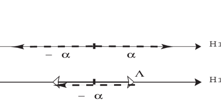
Fig. 1: Root diagram and weight diagram of the fundamental representation of $SU(2)$ where $\mathchar 28931\relax$ is the highest weight of the fundamental representation.

The coherent state for $F_{1}:=SU(2)/U(1)$ is obtained as

$$|j,w\rangle=\xi(w)|j,-j\rangle=e^{\zeta J_{+}-\bar{\zeta}J_{-}}|j,-j\rangle={1\over(1+|w|^{2})^{j}}e^{wJ_{+}}|j,-j\rangle,$$ (3.1)

where $|j,-j\rangle$ is the lowest state, $|j,m=-j\rangle$, of $|j,m\rangle,$ and

$$J_{+}=J_{1}+iJ_{2},\quad J_{-}=J_{+}^{\dagger},\quad w={\zeta\sin|\zeta|\over|\zeta|\cos|\zeta|}.$$ (3.2)

Note that $(1+|w|^{2})^{-j}$ is a normalization factor that ensures $\langle j,w|j,w\rangle=1,$ which is obtained from the Baker-Campbell-Hausdorff (BCH) formulas. The invariant measure is given by

$$d\mu={2j+1\over 4\pi}{dwd\bar{w}\over(1+|w|^{2})^{2}}.$$ (3.3)

For $J_{A}={1\over 2}\sigma^{A}(A=1,2,3)$ with Pauli matrices $\sigma^{A}$, we obtain $J_{+}=\pmatrix{0&1\cr 0&0},$ and

$$e^{wJ_{+}}=\pmatrix{1&w\cr 0&1}\in F_{1}=CP^{1}=SU(2)/U(1)\cong S^{2}.$$ (3.4)

The complex variable $w$ is a $CP^{1}$ variable written as $w=e^{i\phi}\cot{\theta\over 2},$ in terms of the polar coordinate on $S^{2}$ or Euler angles, see Ref.?. We introduce the $O(3)$ vector ${\bf n}$ as

$$n^{1}:=\sin{\theta}\cos{\phi},\quad n^{2}:=\sin{\theta}\sin{\phi},\quad n^{3}:=\cos{\phi}.$$ (3.5)

The relation

$$n^{A}(x)=\bar{\phi}_{a}(x)\sigma_{ab}^{A}\phi_{b}(x)\quad(a,b=1,2)$$ (3.6)

is equivalent to

$$n_{1}=2\Re(\phi_{1}\bar{\phi}_{2}),\quad n_{2}=2\Im(\phi_{1}\bar{\phi}_{2}),\quad n_{3}=|\phi_{1}|^{2}-|\phi_{2}|^{2}.$$ (3.7)

The complex coordinate $w$ obtained by the stereographic projection from the north pole is identical to the inhomogeneous local coordinates of $CP^{1}$ when $\phi_{2}\not=0$,

$$w=w^{(1)}+iw^{(2)}={n_{1}+in_{2}\over 1-n_{3}}={2\phi_{1}\bar{\phi}_{2}\over(|\phi_{1}|^{2}+|\phi_{2}|^{2})-(|\phi_{1}|^{2}-|\phi_{2}|^{2})}={\phi_{1}\over\phi_{2}}.$$ (3.8)

The stereographic projection from the south pole leads to

$$w={n_{1}+in_{2}\over 1+n_{3}}=\left({\phi_{2}\over\phi_{1}}\right)^{*}$$ (3.9)

if $\phi_{1}\not=0$. The variable $w$ is $U(1)$ gauge invariant. Another representation of n is obtained by using the parameterization (3.4) of the $F_{1}$ variable $\xi$:

$$n^{A}=\langle\mathchar 28931\relax|\xi(w)^{\dagger}\sigma^{A}\xi(w)|\mathchar 28931\relax\rangle=\pmatrix{\bar{\phi}_{1}&0}\pmatrix{1&\bar{w}\cr 0&1}\sigma^{A}\pmatrix{1&0\cr w&1}\pmatrix{\phi_{1}\cr 0}.$$ (3.10)

This leads to

$$n_{1}=|\phi_{1}|^{2}(w+\bar{w}),\quad n_{2}=-i|\phi_{1}|^{2}(w-\bar{w}),\quad n_{3}=|\phi_{1}|^{2}(1-w\bar{w}).$$ (3.11)

Indeed, this agrees with (3.7) if $w=({\phi_{2}\over\phi_{1}})^{*}$. The entire space of $F_{1}$ is covered by two charts,

$$CP^{1}=U_{1}\cup U_{2},\quad U_{a}=\{(\phi_{1},\phi_{2})\in CP^{1};\phi_{a}\not=0\}.$$ (3.12)

3.2 $SU(3)$ coherent state

For concreteness, we first focus on the $SU(3)$ case. The general $SU(N)$ case will be discussed in the final part of this section. The highest weight $\mathchar 28931\relax$ of the representation specified by the Dynkin index $[m,n]$ can be written as

$$\vec{\mathchar 28931\relax}=m\vec{h}_{1}+n\vec{h}_{2},$$ (3.13)

where $m$ and $n$ are non-negative integers for the highest weight and $h_{1}$ and $h_{2}$ are the highest weights of the two fundamental representations of $SU(3)$ corresponding to $[1,0]$ and $[0,1]$, respectively (see Fig.2)

$$\vec{h}_{1}=\left({1\over 2},{1\over 2\sqrt{3}}\right),\quad\vec{h}_{2}=\left(0,{1\over\sqrt{3}}\right).$$ (3.14)

Therefore, we obtain

$$\vec{\mathchar 28931\relax}=\left({m\over 2},{m+2n\over 2\sqrt{3}}\right).$$ (3.15)

The generators of SU(3) in the Cartan basis are written as $\{H_{1},H_{2},E_{\alpha},E_{\beta},E_{\alpha+\beta},$ $E_{-\alpha},E_{-\beta},E_{-\alpha-\beta}\}$, where $\alpha$ and $\beta$ are the two simple roots. (See Fig.3 for the explicit choice.)

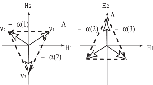
Fig. 2: The weight diagram and root vectors required to define the coherent state in the fundamental representations $[1,0]={\bf 3}$, $[0,1]={\bf 3}^{*}$ of $SU(3)$ where $\vec{\mathchar 28931\relax}=\vec{h}_{1}=\nu^{1}:=({1\over 2},{1\over 2\sqrt{3}})$ is the highest weight of the fundamental representation, and the other weights are $\nu^{2}:=(-{1\over 2},{1\over 2\sqrt{3}})$ and $\nu^{3}:=(0,-{1\over\sqrt{3}})$.

If $mn=0$, ($m=0$ or $n=0$), the maximal stability group $\tilde{H}$ is given by $\tilde{H}=U(2)$ with generators $\{H_{1},H_{2},E_{\beta},E_{-\beta}\}$ (case (I)). Such a degenerate case occurs when the highest-weight vector $\vec{\mathchar 28931\relax}$ is orthogonal to some root vectors (see Fig.2). If $mn\not=0$ ($m\not=0$ and $n\not=0$), $H$ is the maximal torus group $\tilde{H}=U(1)\times U(1)$ with generators $\{H_{1},H_{2}\}$ (case (II)). This is a non-degenerate case (see Fig.4). Therefore, for the highest weight $\mathchar 28931\relax$ in case (I), the coset $G/\tilde{H}$ is given by

$$SU(3)/U(2)=SU(3)/(SU(2)\times U(1))=CP^{2},$$ (3.16)

whereas in case (II),

$$SU(3)/(U(1)\times U(1))=F_{2}.$$ (3.17)

Here, $CP^{n}$ is the complex projective space and $F_{n}$ is the flag space.[23] Therefore, the two fundamental representations belong to case (I), and hence the maximal stability group is $U(2)$, rather than the maximal torus group $U(1)\times U(1)$. The implications of this fact for the mechanism of quark confinement is discussed in subsequent sections.

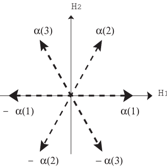
Fig. 3: The root diagram of $SU(3)$, where positive root vectors are given by $\alpha^{(1)}=(1,0)$, $\alpha^{(2)}=({1\over 2},{\sqrt{3}\over 2})$, and $\alpha^{(3)}=({-1\over 2},{\sqrt{3}\over 2})$. Here we have used the same weight ordering as in the $SU(N)$ case (see (3.45)) in defining the simple roots. Then the two simple roots are given by $\alpha^{1}:=\alpha=\alpha^{(1)},$ and $\alpha^{2}:=\beta=\alpha^{(3)}$.

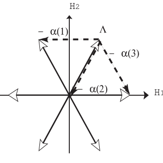
Fig. 4: The weight diagram and root vectors required to define the coherent state in the adjoint representation $[1,1]={\bf 8}$ of $SU(3)$, where $\mathchar 28931\relax=({1\over 2},{\sqrt{3}\over 2})$ is the highest weight of the adjoint representation.

The coherent state for $F_{2}=SU(3)/U(1)^{2}$ is given by

$$|\xi,\mathchar 28931\relax\rangle=\xi(w)|\mathchar 28931\relax\rangle:=V^{\dagger}(w)|\mathchar 28931\relax\rangle,$$ (3.18)

with the highest- (lowest-) weight state $|\mathchar 28931\relax\rangle$, i.e.,

$$|\xi,\mathchar 28931\relax\rangle = \exp\left[\sum_{\alpha\in R_{+}}(\zeta_{\alpha}E_{-\alpha}-\bar{\zeta}_{\alpha}E_{-\alpha}^{\dagger})\right]|\mathchar 28931\relax\rangle$$ (3.19)

$$= e^{-{1\over 2}K(w,\bar{w})}\exp\left[\sum_{\alpha\in R_{+}}\tau_{\alpha}E_{-\alpha}\right]|\mathchar 28931\relax\rangle,$$

where $e^{-{1\over 2}K}$ is the normalization factor obtained from the Kähler potential (explained below):

$$K(w,\bar{w}) := \ln[(\mathchar 28929\relax_{1}(w,\bar{w}))^{m}(\mathchar 28929\relax_{2}(w,\bar{w}))^{n}],$$ (3.20)

$$\mathchar 28929\relax_{1}(w,\bar{w}) := 1+|w_{1}|^{2}+|w_{2}|^{2},\mathchar 28929\relax_{2}(w,\bar{w}):=1+|w_{3}|^{2}+|w_{2}-w_{1}w_{3}|^{2}.$$ (3.21)

The coherent state $|\xi,\mathchar 28931\relax\rangle$ is normalized, so that $\langle\xi,\mathchar 28931\relax|\xi,\mathchar 28931\relax\rangle=1.$ We show in Appendix A that the inner product is given by

$$\langle\xi^{\prime},\mathchar 28931\relax|\xi,\mathchar 28931\relax\rangle=e^{K(w,\bar{w}^{\prime})}e^{-{1\over 2}[K(w^{\prime},\bar{w}^{\prime})+K(w,\bar{w})]},$$ (3.22)

where

$$K(w,\bar{w}^{\prime}):=\ln[1+\bar{w}_{1}{}^{\prime}w_{1}+\bar{w}_{2}{}^{\prime}w_{2}]^{m}[1+\bar{w}_{3}{}^{\prime}w_{3}+(\bar{w}_{2}{}^{\prime}-\bar{w}_{1}{}^{\prime}\bar{w}_{3}{}^{\prime})(w_{2}-w_{1}w_{3})]^{n}.$$ (3.23)

Note that $K(w,\bar{w}^{\prime})$ reduces to the Kähler potential $K(w,\bar{w})$ when $w^{\prime}=w$, in agreement with the normalization. It follows from the general formula (see discussion of the $SU(N)$ case) that the $SU(3)$ invariant measure is given (up to a constant factor) by

$$d\mu(\xi)=d\mu(w,\bar{w})=D(m,n)[(\mathchar 28929\relax_{1})^{m}(\mathchar 28929\relax_{2})^{n}]^{-2}\prod_{\alpha=1}^{3}dw_{\alpha}d\bar{w}_{\alpha},$$ (3.24)

where $D(m,n)={1\over 2}(m+1)(n+1)(m+n+2)$ is the dimension of the representation. For the choice of shift-up $(E_{+i})$ or shift-down $(E_{-i})$ operators

$$E_{\pm 1}:=\frac{\lambda_{1}\pm i\lambda_{2}}{2\sqrt{2}},\quad E_{\pm 2}:=\frac{\lambda_{4}\pm i\lambda_{5}}{2\sqrt{2}},\quad E_{\pm 3}:=\frac{\lambda_{6}\pm i\lambda_{7}}{2\sqrt{2}},$$ (3.25)

with the Gell-Mann matrices $\lambda_{A}(A=1,\cdots,8)$, we obtain

$$\exp\left[\sum_{i=1}^{3}\tau_{i}E_{-i}\right]=\pmatrix{1&w_{1}&w_{2}\cr 0&1&w_{3}\cr 0&0&1}^{t}\in F_{2}=SU(3)/U(1)^{2},$$ (3.26)

where we have used the abbreviation $E_{\pm i}\equiv E_{\pm\alpha^{(i)}}\ (i=1,2,3)$. These two sets of three complex variables are related as (see Appendix A)

$$w_{1}=\frac{\tau_{1}}{\sqrt{2}},\quad w_{2}=\frac{\tau_{2}}{\sqrt{2}}+\frac{\tau_{1}\tau_{3}}{4},\quad w_{3}=\frac{\tau_{3}}{\sqrt{2}},$$ (3.27)

or conversely

$$\tau_{1}=\sqrt{2}w_{1},\quad\tau_{2}=\sqrt{2}\left(w_{2}-\frac{w_{1}w_{3}}{2}\right),\quad\tau_{3}=\sqrt{2}w_{3}.$$ (3.28)

The complex projective space $CP^{2}$ is covered by three complex planes ${\bf C}$ through holomorphic maps [33] (see Appendix B). The parameterization of $SU(3)$ in terms of eight angles is also possible in $SU(3)$, just as $SU(2)$ is parameterized by three Euler angles (see Ref.?).

3.3 $SU(N)$ case

For $SU(N)=SU(n+1)$, the flag space [23] is defined by

$$F_{n}=SU(n+1)/U(1)^{n}\ni V.$$ (3.29)

We use $V$ to denote an element of $F_{n}$ in this definition. $F_{n}$ is a compact Kähler manifold,[35, 36] which is a homogeneous but nonsymmetric manifold of dimension ${\rm dim}_{\bf C}F_{n}=n(n+1)/2$.

Since the flag manifold $F_{n}$ is a Kähler manifold,[35, 36] it possesses complex local coordinates $w_{\alpha}$, a Hermitian Riemannian metric,

$$ds^{2}=g_{\alpha\bar{\beta}}dw^{\alpha}d\bar{w}^{\beta},$$ (3.30)

and a corresponding two-form, called the Kähler form,

$$\mathchar 28938\relax_{K}=ig_{\alpha\bar{\beta}}dw^{\alpha}\wedge d\bar{w}^{\beta},$$ (3.31)

which is closed, i.e.,

$$d\mathchar 28938\relax_{K}=0.$$ (3.32)

Any closed form $\mathchar 28938\relax_{K}$ is locally exact ($\mathchar 28938\relax_{K}=d\omega$), due to Poincaré’s lemma. The condition (3.32) is equivalent to

$${\partial g_{\alpha\bar{\beta}}\over\partial w^{\gamma}}={\partial g_{\gamma\bar{\beta}}\over\partial w^{\alpha}},\quad{\rm or}\quad{\partial g_{\alpha\bar{\beta}}\over\partial\bar{w}^{\gamma}}={\partial g_{\alpha\bar{\gamma}}\over\partial\bar{w}^{\beta}}.$$ (3.33)

This holds if and only if the metric $g_{\alpha\beta}$ can be obtained from a real scalar function $K$ as

$$g_{\alpha\bar{\beta}}={\partial\over\partial w^{\alpha}}{\partial\over\partial\bar{w}^{\beta}}K,$$ (3.34)

where $K=K(w,\bar{w})$ is called the Kähler potential. Then the Kähler two-form is obtained from (3.31) as

$$\mathchar 28938\relax_{K}=i\partial\bar{\partial}K.$$ (3.35)

On the flag space, there transitively act two groups, $G=SU(n+1)$ and its complexification $G^{c}=SL(n+1,{\bf C})$. Any element of $F_{n}$ can be written as an upper triangular $(n+1)\times(n+1)$ matrix, whose main diagonal elements are all $1$ and whose upper $n(n+1)/2$ elements are complex numbers, $w_{\alpha}\in{\bf C}$:

$$\xi=\pmatrix{1&w_{1}&w_{2}&\cdots&\cdots&w_{n}\cr 0&1&w_{n+1}&\cdots&\cdots&w_{2n-1}\cr 0&0&1&w_{2n}&\cdots&w_{3n-3}\cr&&&&&\cr\vdots&\vdots&\vdots&\vdots&\vdots&\vdots\cr&&&&&\cr 0&0&\cdots&0&1&w_{n(n+1)/2}\cr 0&0&\cdots&\cdots&0&1\cr}\in F_{n}.$$ (3.36)

Therefore, we can write

$$F_{n}=SL(n+1,{\bf C})/B_{-}\ni\xi,$$ (3.37)

where $B_{-}(B_{+})$ is the Borel subgroup, i.e., the group of lower (upper) triangular matrices with determinant equal to $1$ (Iwasawa decomposition). This definition (3.37) should be compared with the first definition (3.29). The mapping $G/H\rightarrow G^{c}/B_{-}$ is a generalization of the stereographic projection in the $G=SU(2)$ case.[13] The action of the group $SL(n+1,{\bf C})$ on $F_{n}$, $g:V\rightarrow V_{g}$ can be found through the Gauss decomposition,

$$V\cdot g=TDV_{g},\quad g\in SL(n+1,{\bf C}),\quad T\in Z_{-}(n+1),\quad V_{g}\in Z_{+}(n+1),$$ (3.38)

where $Z_{+}(n+1)(Z_{-}(n+1))$ is the set of upper (lower) triangular matrices whose main diagonal elements are all $1$ and $D$ is a diagonal matrix with determinant equal to 1. The elements of the factors $T,D$ and $V_{g}$ are rational functions of the elements of $g$.

The group $G=SU(N)$ has rank $N-1$, and the Cartan subalgebra is constructed from $(N-1)$ diagonal generators $H_{i}$. Hence, there are $N(N-1)$ off-diagonal shift operators $E_{\alpha}$, since ${\rm dim}SU(N):=N^{2}-1=(N-1)+N(N-1)$. Therefore, the total number of roots is $N(N-1)$, of which there are $N-1$ simple roots. Other roots are constructed as linear combination of the simple roots. Also, there are $N$ weight vectors. An element of $SU(N)$ is represented by the $N\times N$ unitary matrices with determinant $1$ that are generated by traceless Hermitian matrices, $N^{2}-1$ linearly independent generators $T^{A}(A=1,\cdots,N^{2}-1)$. The generators are normalized as

$${\rm tr}(T^{A}T^{B})={1\over 2}\delta_{AB}.$$ (3.40)

Each off-diagonal generator $E_{\alpha}$ has a single non-zero element $1/\sqrt{2}$. The diagonal generator $H_{m}$ is defined by

$$(H_{m})_{ab} = {1\over\sqrt{2m(m+1)}}(\sum_{k=1}^{m}\delta_{ak}\delta_{bk}-m\delta_{a,m+1}\delta_{b,m+1})$$ (3.41)

$$= {1\over\sqrt{2m(m+1)}}{\rm diag}(1,\cdots,1,-m,0,\cdots,0).$$ (3.42)

For $m=1$ to $N-1$, the first $m$ diagonal elements (beginning from the upper left-hand corner) of $H_{m}$ are $1$, the next one is $-m$, and the rest of the diagonal elements are $0$. Thus $H_{m}$ is traceless. The weight vectors (eigenvectors of all $H_{i}$: $H_{j}|\nu\rangle=\nu^{j}|\nu\rangle$) of the fundamental representation ${\bf N}$ ($N$-dimensional irreducible representation of $SU(N)$) are given by [37]

$$\nu^{1} = \left({1\over 2},{1\over 2\sqrt{3}},\cdots,{1\over\sqrt{2m(m+1)}},\cdots,{1\over\sqrt{2(N-1)N}}\right),$$

$$\nu^{2} = \left(-{1\over 2},{1\over 2\sqrt{3}},\cdots,{1\over\sqrt{2m(m+1)}},\cdots,{1\over\sqrt{2(N-1)N}}\right),$$

$$\nu^{3} = \left(0,-{1\over\sqrt{3}},{1\over 2\sqrt{6}},\cdots,{1\over\sqrt{2(N-1)N}}\right),$$

$$\vdots$$

$$\nu^{m+1} = \left(0,0,\cdots,0,-{m\over\sqrt{2m(m+1)}},\cdots,{1\over\sqrt{2(N-1)N}}\right),$$

$$\vdots$$

$$\nu^{N} = \left(0,0,\cdots,0,{-N+1\over\sqrt{2(N-1)N}}\right).$$ (3.43)

All the weight vectors have the same length, and the angles between different weights are the same:

$$\nu^{i}\cdot\nu^{i}={N-1\over 2N},\quad\nu^{i}\cdot\nu^{j}=-{1\over 2N}\quad({\rm for}i\not=j).$$ (3.44)

The weights constitute a polygon in the $N-1$ dimensional space. This implies that any weight can be used as the highest weight. A weight will be called positive if its last non-zero component is positive. With this definition, the weights satisfy

$$\nu^{1}>\nu^{2}>\cdots>\nu^{N}.$$ (3.45)

The simple roots are given by

$$\alpha^{i}=\nu^{i}-\nu^{i+1}\quad(i=1,\cdots,N-1)$$ (3.46)

Explicitly, we have

$$\alpha^{1} = \left(1,0,\cdots,0\right),$$

$$\alpha^{2} = \left(-{1\over 2},{\sqrt{3}\over 2},0,\cdots,0\right),$$

$$\alpha^{3} = \left(0,-{1\over\sqrt{3}},\sqrt{{2\over 3}},0,\cdots,0\right),$$

$$\vdots$$

$$\alpha^{m} = \left(0,0,\cdots,-\sqrt{{m-1\over 2m}},\sqrt{{m+1\over 2m}},0,\cdots,0\right),$$

$$\vdots$$

$$\alpha^{N-1} = \left(0,0,\cdots,-\sqrt{{N-2\over 2(N-1)}},\sqrt{{N\over 2(N-1)}}\right).$$ (3.47)

As can be shown from (3.44), all these roots have length 1, the angles between successive roots are the same, $2\pi/3$, and other roots are orthogonal:

$$\alpha^{j}\cdot\alpha^{j}=1,\quad\alpha^{i}\cdot\alpha^{j}=-{1\over 2},\quad(j=i\pm 1)$$ (3.48)

$$\alpha^{i}\cdot\alpha^{j}=0.\quad(j\not=i,i\pm 1)$$ (3.49)

This fact is usually expressed by a Dynkin diagram (see Fig.5).

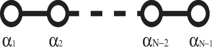
Fig. 5: The Dynkin diagram of $SU(N)$.

If we choose $\nu^{1}$ as the highest-weight $\vec{\mathchar 28931\relax}$ of the fundamental representation ${\bf N}$, some of the roots are orthogonal to $\nu^{1}$. From the above construction, it is easy to see that only one simple root $\alpha_{1}$ is not-orthogonal to $\nu^{1}$, and that all the other simple roots are orthogonal:

$$\nu^{1}\cdot\alpha^{1}\not=0,\quad\nu^{1}\cdot\alpha^{2}=\nu^{1}\cdot\alpha^{3}=\cdots=\nu^{1}\cdot\alpha^{N-1}=0.$$ (3.50)

Therefore, all the linear combinations constructed from $\alpha^{2},\cdots,\alpha^{N-1}$ are also orthogonal to $\nu^{1}$. Non-orthogonal roots are obtained only when $\alpha^{1}$ is included in the linear combinations. It is not difficult to show that the total number of non-orthogonal roots is $2(N-1)$, and hence there are $N(N-1)-2(N-1)=(N-2)(N-1)$ orthogonal roots. The $(N-2)(N-1)$ shift operators $E_{\alpha}$ corresponding to these orthogonal roots together with the $N-1$ Cartan subalgebra $H_{i}$ constitute the maximal stability subgroup $\tilde{H}=U(N-1)$, since $(N-2)(N-1)+(N-1)=(N-1)^{2}={\rm dim}U(N-1)$. Thus, for the fundamental representation, the stability subgroup $\tilde{H}$ of $SU(N)$ is given by $\tilde{H}=U(N-1)$. In order to describe the coset space $G/\tilde{H}$, we need only $(N-1)$ complex numbers, since

$$G/\tilde{H}=SU(N)/U(N-1),$$ (3.51)

and ${\rm dim}G/\tilde{H}=2(N-1)$. We conclude that $G/\tilde{H}=CP^{N-1}$, where $CP^{N-1}$ is the $(N-1)$-dimensional complex projective space,[35, 36, 33, 38] which is a submanifold of the flag manifold $F_{N-1}$.

The complex projective space $CP^{n}$ is the compact Kähler symmetric space with ${\rm dim}_{\bf C}CP^{n}=n$. The $SU(n+1)$ group can act transitively on this manifold, and this manifold can be considered as a factor space:

$${\bf C}P^{n}=SU(n+1)/(SU(n)\times U(1)).$$ (3.52)

An element of $CP^{n}$ can be expressed using the $n$ complex variables $w_{1},\cdots,w_{n}$ as

$$\pmatrix{1&w_{1}&w_{2}&\cdots&\cdots&w_{n}\cr 0&1&0&\cdots&\cdots&0\cr 0&0&1&0&\cdots&0\cr&&&&&\cr\vdots&\vdots&\vdots&\vdots&\vdots&\vdots\cr&&&&&\cr 0&0&\cdots&0&1&0\cr 0&0&\cdots&\cdots&0&1\cr}\in CP^{n}.$$ (3.53)

The Kähler potential of $F_{n}$ ($n=N-1$) is obtained as follows. Let $H$ be the Hermitian matrix defined by $H=VV^{\dagger},V\in F_{n}$. Consider the Gauss decomposition

$$H=VV^{\dagger}=TDV,$$ (3.54)

where $T\in Z_{-}(n+1)$ and $D$ is a diagonal matrix with determinant equal to 1. $H$ has the upper principal minors $\mathchar 28929\relax_{\ell}(VV^{\dagger})(\ell=1,\cdots,n+1)$, which are equal to the following products of the elements $\delta_{\ell}$ of the diagonal matrix $D={\rm diag}(\delta_{1},\cdots,\delta_{n})$:

$$\mathchar 28929\relax_{1}=\delta_{1},\quad\mathchar 28929\relax_{2}=\delta_{1}\delta_{2},\quad\cdots,\quad\mathchar 28929\relax_{n}=\delta_{1}\delta_{2}\cdots\delta_{n},\quad\mathchar 28929\relax_{n+1}=1.$$ (3.55)

Let $d_{\ell}$ $(\ell=1,\cdots,n)$ be the Dynkin index of $SU(n+1)$. Then the Kähler potential of $F_{n}$ is given in the form,

$$K(w,\bar{w})=\sum_{\ell=1}^{n}d_{\ell}K_{\ell}(w,\bar{w})=\sum_{\ell=1}^{n}d_{\ell}\ln\mathchar 28929\relax_{\ell}(w,\bar{w})=\ln\left[\prod_{\ell=1}^{n}(\mathchar 28929\relax_{\ell}(w,\bar{w}))^{d_{\ell}}\right].$$ (3.56)

The function $K(w,\bar{w}^{\prime})$ can also be obtained from the Gauss decomposition of $VV^{\prime\dagger}$:

$$K(w,\bar{w}^{\prime})=\ln\left[\prod_{\ell=1}^{n}(\mathchar 28929\relax_{\ell}(w,\bar{w}^{\prime}))^{d_{\ell}}\right].$$ (3.57)

The $SU(n+1)$ invariant measure on $F_{n}$ is written, up to a multiplicative factor, as [39]

$$d\mu(V,\bar{V})=\rho(V,\bar{V})\prod_{\alpha=1}^{n(n+1)/2}dw_{\alpha}d\bar{w}_{\alpha},$$ (3.58)

$$\rho(V,\bar{V})=\left[\prod_{\ell=1}^{n}\mathchar 28929\relax_{\ell}^{d_{\ell}}\right]^{-2}=\left[\prod_{\ell=1}^{n}\mathchar 28929\relax_{\ell}\right]^{-2},$$ (3.59)

where $d_{\ell}=1$ for all $\ell$. The density $\rho$ of the invariant measure is calculated [23] from

$$\rho=\det(g_{\alpha\bar{\beta}})=\det\left({\partial^{2}K\over\partial w^{\alpha}\partial\bar{w}^{\beta}}\right).$$ (3.60)

The Kähler potential of the $CP^{N-1}$ manifold is given by

$$K=m\ln\left(1+\sum_{\alpha=1}^{N-1}|w_{\alpha}|^{2}\right)=m\ln\left(1+|||w|||^{2}\right),$$ (3.61)

where

$$|||w|||^{2}:=\sum_{a=1}^{N-1}|w_{a}|^{2}.$$ (3.62)

Hence, the metric reads

$$g_{\alpha\bar{\beta}}=m{(1+|||w|||^{2})\delta_{\alpha\beta}-\bar{w}_{\alpha}w_{\beta}\over(1+|||w|||^{2})^{2}}.$$ (3.63)

The above construction of the coherent state can be extended to an arbitrary compact semi-simple Lie group (see Chapter 11 of Perelomov [40]).

4 Non-Abelian Stokes theorem

In this section we derive a new version of the non-Abelian Stokes theorem (NAST) based on the coherent state obtained in the previous section. An advantage of this version of NAST is that it is possible to separate the magnetic monopole contribution in the Wilson loop and that it is very helpful to understand the dual superconductor picture of quark confinement in QCD.

4.1 Non-Abelian Stokes theorem for $SU(N)$

We consider the infinitesimal deviation $\xi^{\prime}=\xi+d\xi$ (which is sufficient to derive the path integral formula). From (3.19),

$$|\xi,\mathchar 28931\relax\rangle=\xi|\mathchar 28931\relax\rangle=e^{-{1\over 2}K(w,\bar{w})}\exp\left[\sum_{\alpha}\tau_{\alpha}(w)E_{-\alpha}\right]|\mathchar 28931\relax\rangle,$$ (4.1)

we find

$$\langle\xi+d\xi,\mathchar 28931\relax|\xi,\mathchar 28931\relax\rangle = \exp[i\omega+O((dw)^{2})],$$ (4.2)

$$\omega(x) := \langle\mathchar 28931\relax|i\xi^{\dagger}(x)d\xi(x)|\mathchar 28931\relax\rangle,$$ (4.3)

where $d$ denotes the exterior derivative

$$d:=dx^{\mu}{\partial\over\partial x^{\mu}}:=dx^{\mu}\partial_{\mu}.$$ (4.4)

Then $\omega$ is the one-form

$$\omega=dx^{\mu}\omega_{\mu},\quad\omega_{\mu}=\langle\mathchar 28931\relax|i\xi^{\dagger}(x)\partial_{\mu}\xi(x)|\mathchar 28931\relax\rangle.$$ (4.5)

Here the $x$ dependence of $\xi$ comes from that of $w(x)$ (the local field variable $w(x)$), i.e., $\xi(x)=\xi(w(x))$.

The exterior derivative is regarded as the operator

$$d=\partial+\bar{\partial}=dw_{\alpha}{\partial\over\partial w_{\alpha}}+d\bar{w}_{\beta}{\partial\over\partial\bar{w}_{\beta}},$$ (4.6)

where the operators $\partial$ and $\bar{\partial}$ are called the Dolbeault operators.[35] From the inner product (3.22),

$$\langle\xi^{\prime},\mathchar 28931\relax|\xi,\mathchar 28931\relax\rangle=e^{K(w,\bar{w}^{\prime})}e^{-{1\over 2}[K(w^{\prime},\bar{w}^{\prime})+K(w,\bar{w})]},$$ (4.7)

we obtain another expression for $\omega$ using the Kähler potential $K$:

$$\omega={i\over 2}(\partial-\bar{\partial})K={i\over 2}\left(dw_{\alpha}{\partial\over\partial w_{\alpha}}-d\bar{w}_{\beta}{\partial\over\partial\bar{w}_{\beta}}\right)K.$$ (4.8)

The Wilson loop operator $W^{C}[{\cal A}]$ is defined as the trace of the path-ordered exponent along the closed loop $C$ as

$$W^{C}[{\cal A}]:={1\over{\cal N}}{\rm tr}\left[{\cal P}\exp\left(ig\oint_{C}{\cal A}\right)\right],$$ (4.9)

where ${\cal N}$ is the dimension of the representation (${\cal N}={\rm dim}({\bf 1}_{R})={\rm tr}({\bf 1}_{R})$), and ${\cal A}$ is the (Lie-algebra valued) connection one-form

$${\cal A}(x)={\cal A}_{\mu}^{A}(x)T^{A}dx^{\mu}={\cal A}^{A}(x)T^{A}.$$ (4.10)

Consider a curve starting from $x_{0}$ and ending at $x$. We parameterize this curve by the parameter $t$ and define

$$W_{ab}(t,t_{0}):=\left[{\cal P}\exp\left(ig\int_{x_{0}(t_{0})}^{x(t)}dx^{\mu}{\cal A}_{\mu}(x)\right)\right]_{ab}=\left[{\cal P}\exp\left(ig\int_{t_{0}}^{t}dt{\cal A}(t)\right)\right]_{ab},$$ (4.11)

where

$${\cal A}(t):={\cal A}_{\mu}(x)dx^{\mu}/dt.$$ (4.12)

Then the wavefunction defined by

$$\psi_{a}(t)=W_{ab}(t,t_{0})\psi_{b}(t_{0})$$ (4.13)

is a solution of the Schrödinger equation

$$\left[i{d\over dt}+g{\cal A}(t)\right]_{ab}\psi_{b}(t)=0.$$ (4.14)

Note that the Wilson loop operator is obtained by taking the trace of (4.11) for the closed loop, say $C$:

$$W^{C}[{\cal A}]={1\over{\cal N}}{\rm tr}(W(t,0))={1\over{\cal N}}\sum_{a=1}^{{\rm dimofrep}}W_{aa}(t,0).$$ (4.15)

This implies [21] that it is possible to write the path integral representation of the Wilson loop operator if we identify ${\cal A}(t)$ with the Hamiltonian as

$$H(t)=-g{\cal A}(t)=-g{\cal A}_{\mu}(x)dx^{\mu}/dt.$$ (4.16)

First, we define the path-ordered exponent by discretizing the time interval $t$ into $N$ infinitesimal steps and subsequently taking the limit $N\rightarrow\infty,\epsilon\rightarrow 0$ with $N\epsilon=t$ fixed as

$${\rm tr}\left\{{\cal P}\exp\left[ig\int_{0}^{t}dt{\cal A}(t)\right]\right\}=\lim_{N\rightarrow\infty,\epsilon\rightarrow 0}{\rm tr}\left\{{\cal P}\prod_{n=0}^{N-1}[1+i\epsilon g{\cal A}(t_{n})]\right\},$$ (4.17)

where $t_{n}:=n\epsilon,\epsilon:=t/N$. For simplicity, we set $t_{0}=0$ and $t_{N}=t$. Next, we use the coherent state $|\xi,\mathchar 28931\relax\rangle$, following Ref.?. On the right-hand-side of (4.17), we replace the trace with

$${1\over{\cal N}}{\rm tr}(\cdots)=\int d\mu(\xi_{N})\langle\xi_{N},\mathchar 28931\relax|(\cdots)|\xi_{N},\mathchar 28931\relax\rangle,$$ (4.18)

and insert the complete set (resolution of unity)

$$I=\int|\xi_{n},\mathchar 28931\relax\rangle d\mu(\xi_{n})\langle\xi_{n},\mathchar 28931\relax|.\quad(n=1,2,\cdots,N-1)$$ (4.19)

Then we obtain

$$\ \ {1\over{\cal N}}{\rm tr}\left\{{\cal P}\exp\left[ig\int_{0}^{t}dt{\cal A}(t)\right]\right\}$$ (4.20)

$$= \lim_{N\rightarrow\infty,\epsilon\rightarrow 0}\int\cdots\int d\mu(\xi_{N})\langle\xi_{N},\mathchar 28931\relax|[1+i\epsilon g{\cal A}(t_{N-1})]|\xi_{N-1},\mathchar 28931\relax\rangle d\mu(\xi_{N-1})$$

$$\times\langle\xi_{N-1},\mathchar 28931\relax|[1+i\epsilon g{\cal A}(t_{N-2})]|\xi_{N-2},\mathchar 28931\relax\rangle d\mu(\xi_{N-2})$$

$$\cdots d\mu(\xi_{1})\langle\xi_{1},\mathchar 28931\relax|[1+i\epsilon g{\cal A}(t_{0})]|\xi_{N},\mathchar 28931\relax\rangle$$

$$= \lim_{N\rightarrow\infty,\epsilon\rightarrow 0}\prod_{n=1}^{N}\int d\mu(\xi_{n})\prod_{n=0}^{N-1}\langle\xi_{n+1},\mathchar 28931\relax|[1+i\epsilon g{\cal A}(t_{n})]|\xi_{n},\mathchar 28931\relax\rangle$$

$$= \lim_{N\rightarrow\infty,\epsilon\rightarrow 0}\prod_{n=1}^{N}\int d\mu(\xi_{n})\prod_{n=0}^{N-1}\left[1+i\epsilon g\bar{A}(t_{n})\right]\prod_{n=0}^{N-1}\langle\xi_{n+1},\mathchar 28931\relax|\xi_{n},\mathchar 28931\relax\rangle$$

$$= \lim_{N\rightarrow\infty,\epsilon\rightarrow 0}\prod_{n=1}^{N}\int d\mu(\xi_{n})\exp\left[i\epsilon\sum_{n=0}^{N-1}g\bar{A}(t_{n})\right]\prod_{n=0}^{N-1}\langle\xi_{n+1},\mathchar 28931\relax|\xi_{n},\mathchar 28931\relax\rangle,$$

where we have used $\xi_{0}=\xi_{N}$ and have defined

$$\bar{A}(t_{n}):={\langle\xi_{n+1},\mathchar 28931\relax|{\cal A}(t_{n})|\xi_{n},\mathchar 28931\relax\rangle\over\langle\xi_{n+1},\mathchar 28931\relax|\xi_{n},\mathchar 28931\relax\rangle}.$$ (4.21)

Up to $O(\epsilon^{2})$, we find

$$\bar{A}(t_{n}):=\langle\xi_{n},\mathchar 28931\relax|{\cal A}(t_{n})|\xi_{n},\mathchar 28931\relax\rangle+O(\epsilon^{2})=\langle\mathchar 28931\relax|\xi(t_{n})^{\dagger}{\cal A}(t_{n})\xi(t_{n})|\mathchar 28931\relax\rangle+O(\epsilon^{2}),$$ (4.22)

and

$$\langle\xi_{n+1},\mathchar 28931\relax|\xi_{n},\mathchar 28931\relax\rangle = \langle\xi(t_{n}),\mathchar 28931\relax|\xi(t_{n}),\mathchar 28931\relax\rangle+\epsilon\langle\dot{\xi}(t_{n}),\mathchar 28931\relax|\xi(t_{n}),\mathchar 28931\relax\rangle+O(\epsilon^{2})$$ (4.23)

$$= \exp[\epsilon\langle\dot{\xi}(t_{n}),\mathchar 28931\relax|\xi(t_{n}),\mathchar 28931\relax\rangle+O(\epsilon^{2})]$$

$$= \exp[-i\epsilon\langle\mathchar 28931\relax|i\dot{\xi}(t_{n})^{\dagger}\xi(t_{n})|\mathchar 28931\relax\rangle+O(\epsilon^{2})]$$

$$= \exp[i\epsilon\langle\mathchar 28931\relax|i\xi(t_{n})^{\dagger}\dot{\xi}(t_{n})|\mathchar 28931\relax\rangle+O(\epsilon^{2})],$$

where we have used $\langle\xi(t_{n}),\mathchar 28931\relax|\xi(t_{n}),\mathchar 28931\relax\rangle=1$. Therefore we arrive at the expression

$$W^{C}[{\cal A}] = \lim_{N\rightarrow\infty,\epsilon\rightarrow 0}\prod_{n=1}^{N}\int d\mu(\xi(t_{n}))$$ (4.24)

$$\times \exp\left\{ig\epsilon\sum_{n=0}^{N-1}\langle\mathchar 28931\relax|[\xi(t_{n})^{\dagger}{\cal A}(t_{n})\xi(t_{n})+ig^{-1}\xi(t_{n})^{\dagger}\dot{\xi}(t_{n})]|\mathchar 28931\relax\rangle\right\}.$$

Thus we obtain the path integral representation of the Wilson loop,

$$W^{C}[{\cal A}] = \int[d\mu(\xi)]_{C}\exp\left(ig\oint_{C}\langle\mathchar 28931\relax|\left[V{\cal A}V^{\dagger}+{i\over g}VdV^{\dagger}\right]|\mathchar 28931\relax\rangle\right),$$ (4.25)

where $[d\mu(\xi)]_{C}$ is the product measure of $d\mu(w(x),\bar{w}(x))$ along the loop $C$:

$$[d\mu(\xi)]_{C}:=\lim_{N\rightarrow\infty,\epsilon\rightarrow 0}\prod_{n=1}^{N}\int d\mu(\xi_{n}).$$ (4.26)

Using the (usual) Stokes theorem, $\oint_{C=\partial S}\omega=\int_{S}d\omega,$ we obtain the non-Abelian Stokes theorem (NAST):

$$W^{C}[{\cal A}] = \int[d\mu(\xi)]_{C}\exp\left(ig\oint_{C}\left[n^{A}{\cal A}^{A}+{1\over g}\omega\right]\right)$$ (4.27)

$$= \int[d\mu(\xi)]_{C}\exp\left(ig\int_{S:\partial S=C}\left[d(n^{A}{\cal A}^{A})+{1\over g}\mathchar 28938\relax_{K}\right]\right).$$

Here we have defined

$$n^{A}(x) := \langle\mathchar 28931\relax|\xi^{\dagger}(x)T^{A}\xi(x)|\mathchar 28931\relax\rangle,$$ (4.28)

$$\omega(x) := \langle\mathchar 28931\relax|i\xi^{\dagger}(x)d\xi(x)|\mathchar 28931\relax\rangle,$$ (4.29)

and

$$\mathchar 28938\relax_{K}:=d\omega.$$ (4.30)

Taking into account (4.8), we find that this $\mathchar 28938\relax_{K}$ is identical to the Kähler two-form, in agreement with the general statement (3.35), i.e.,

$$\mathchar 28938\relax_{K}=d\omega=(\partial+\bar{\partial}){i\over 2}(\partial-\bar{\partial})K=i\partial\bar{\partial}K,$$ (4.31)

since the identity $d^{2}=0$ leads to $\partial^{2}=0=\bar{\partial}^{2},\partial\bar{\partial}+\bar{\partial}\partial=0.$ Therefore, the second term, $\omega$ or $\mathchar 28938\relax_{K}$, in the exponent of the NAST is entirely determined from the Kähler potential of the flag manifold.

For $SU(N)$, the topological part,

$$\gamma:=\oint_{C}\omega=\int_{S}\mathchar 28938\relax_{K},$$ (4.32)

corresponding to the residual $U(N-1)$ invariance is interpreted as the geometric phase of the Wilczek-Zee holonomy, [41] just as in the $SU(2)$ case it is interpreted as the Berry-Aharonov-Anandan phase for the residual $U(1)$ invariance. The details of this point will be given in a subsequent article.[42]

4.2 Fundamental representation of $SU(N)$ and $CP^{N-1}$ variable

Defining

$$\omega_{a}(x):=(V^{\dagger}(x)|\mathchar 28931\relax\rangle)_{a},\quad(a=1,\cdots,N)$$ (4.33)

we can write

$$n^{A}(x):=\langle\mathchar 28931\relax|V(x)T^{A}V^{\dagger}(x)|\mathchar 28931\relax\rangle=\bar{\omega}_{a}(x)(T^{A})_{ab}\omega_{b}(x).$$ (4.34)

In the $CP^{N-1}$ case, in particular, the highest-weight state is given by a column vector,

$$|\mathchar 28931\relax\rangle=\pmatrix{1\cr 0\cr\vdots\cr 0},$$ (4.35)

and then we can write

$$n^{A}(x):=\langle\mathchar 28931\relax|U(x)T^{A}U^{\dagger}(x)|\mathchar 28931\relax\rangle=\bar{\phi}_{a}(x)(T^{A})_{ab}\phi_{b}(x),$$ (4.36)

where $U\in SU(N)$ and

$$\phi_{a}(x) := (U^{\dagger}(x)|\mathchar 28931\relax\rangle)_{a}={\bar{U}}_{1a}(x).$$ (4.37)

Then $n^{A}(x)$ can be rewritten as

$$n^{A}(x) = (U(x)T^{A}U^{\dagger}(x))_{11}.$$ (4.38)

Note that the $CP^{N-1}$ variables $\phi_{a}(a=1,\cdots,N)$ are subject to the constraint

$$\sum_{a=1}^{N}|\phi_{a}(x)|^{2}=1.$$ (4.39)

This is clearly satisfied by the unitarity of $U$, $\sum_{a=1}^{N}U_{1a}(x){\bar{U}}_{1a}(x)=(U(x)U^{\dagger}(x))_{11}=1.$

Now, we examine another expression (the adjoint orbit representation),

$$n^{A}(x)=2{\rm tr}(U^{\dagger}(x){\cal H}U(x)T^{A}),$$ (4.40)

or equivalently,

$${\bf n}(x):=n^{A}(x)T^{A}=U^{\dagger}(x){\cal H}U(x).$$ (4.41)

Here ${\cal H}$ is defined by

$${\cal H}=\vec{\mathchar 28931\relax}\cdot(H^{1},\cdots,H^{N-1})=\sum_{i=1}^{N-1}\mathchar 28931\relax^{i}H^{i}={1\over 2}{\rm diag}\left(\frac{N-1}{N},-\frac{1}{N},\cdots,-\frac{1}{N}\right),$$ (4.42)

where we have used (3.42) and

$$\mathchar 28931\relax^{i}={1\over\sqrt{2i(i+1)}}.$$ (4.43)

For $SU(3)$, when the Dynkin index $[m,n]=[1,0]$ or $[0,1]$, (4.42) reduces to

$${\cal H}=\vec{\mathchar 28931\relax}\cdot\left(\frac{\lambda^{3}}{2},\frac{\lambda^{8}}{2}\right)={1\over 2}{\rm diag}\left({2\over 3},-{1\over 3},-{1\over 3}\right),\quad{\rm or}\quad{1\over 2}{\rm diag}\left({1\over 3},{1\over 3},-{2\over 3}\right).$$ (4.44)

Note that two elements agree with each other. Hence the adjoint orbit cannot cover all the flag space $F_{2}$. This is the $CP^{2}$ case. It is easy to see that the two definitions (4.36) and (4.40) are equivalent,

$$n^{A}(x)=(U(x)T^{A}U^{\dagger}(x))_{11}=2{\rm tr}({\cal H}U(x)T^{A}U^{\dagger}(x)),$$ (4.45)

since $UT^{A}U^{\dagger}$ is traceless.

The correspondence between the $F_{N-1}$ variables $w_{a}$ and the $CP^{N-1}$ variables $\phi_{a}$ is given, e.g., by

$$\phi_{1}=w_{1},\quad\phi_{2}=w_{2},\quad\cdots,\quad\phi_{N-1}=w_{N-1},\quad\phi_{N}=1.$$ (4.46)

Thus $\omega$ is an inhomogeneous coordinate, $\omega_{a}=\phi_{a}/\phi_{N}=w_{a}$ ($a=1,\cdots,N-1$), by definition. In the $CP^{N-1}$ case (for the fundamental representation), we can perform the replacement

$$\langle\mathchar 28931\relax|f(V)|\mathchar 28931\relax\rangle=2{\rm tr}[{\cal H}f(U)]$$ (4.47)

if $f(V)$ belongs to the Lie algebra of $G$ (and hence $f(V)$ is traceless, i.e., ${\rm tr}f(V)=0$). Thus, we obtain another expression for $\omega$,

$$\omega(x):=2{\rm tr}[{\cal H}iU(x)dU^{\dagger}(x)]=-i2{\rm tr}[{\cal H}dU(x)U^{\dagger}(x)],$$ (4.48)

which is a diagonal piece of the Maurer-Cartan one-form,

$$\vartheta:=dUU^{-1}.$$ (4.49)

It turns out that the two-form $\mathchar 28938\relax_{K}$ is the symplectic two-form,

$$\mathchar 28938\relax_{K}=d\omega=2{\rm tr}({\cal H}[U^{-1}dU,U^{-1}dU])=2{\rm tr}({\bf n}[d{\bf n},d{\bf n}]).$$ (4.50)

Our choice of ${\cal H}$ is the most economical one (see Ref.? for different choices and more discussion of the related issues).

From the Kähler potential of $CP^{N-1}$ (3.61) and the relation (4.8), the connection one-form $\omega$ reads

$$\omega:={i\over 2}{\bar{w}_{\alpha}dw_{\alpha}-d\bar{w}_{\alpha}w_{\alpha}\over 1+\bar{w}_{\alpha}w_{\alpha}},$$ (4.51)

which is equal to

$$\omega:=i{\bar{w}_{\alpha}dw_{\alpha}\over 1+\bar{w}_{\alpha}w_{\alpha}},$$ (4.52)

up to the total derivative. By taking the exterior derivative, we obtain

$$\mathchar 28938\relax_{K}=d\omega=i{(1+|||w|||^{2})\delta_{\alpha\beta}-\bar{w}_{\alpha}w_{\beta}\over(1+|||w|||^{2})^{2}}dw^{\alpha}\wedge d\bar{w}^{\beta},$$ (4.53)

which agrees with the metric (3.63).

4.3 An implication of the NAST

The NAST (4.27) implies that the Wilson loop operator is given by

$$W^{C}[{\cal A}]=\int[d\mu(\xi)]_{C}\exp\left(ig\oint_{C}a\right)=\int[d\mu(\xi)]_{C}\exp\left(ig\int_{S:C=\partial S}f\right).$$ (4.54)

First, $a$ is the connection one-form

$$a:=n^{A}{\cal A}^{A}+{1\over g}\omega=\langle\mathchar 28931\relax|{\cal A}^{V}|\mathchar 28931\relax\rangle,$$ (4.55)

where ${\cal A}^{V}$ is obtained as the gauge transformation of ${\cal A}$ by $V\in F_{N-1}$:

$${\cal A}^{V}:=V{\cal A}V^{\dagger}+{i\over g}VdV^{\dagger}=\xi^{\dagger}{\cal A}\xi+{i\over g}\xi^{\dagger}d\xi.$$ (4.56)

For a quark in the fundamental representation, we can write

$$a=2{\rm tr}({\cal H}{\cal A}^{V}).$$ (4.57)

Therefore, the one-form $a$ is equal to the diagonal piece of the gauge-transformed potential ${\cal A}^{V}$. This fact is very useful to derive the Abelian dominance in the low-energy physics of QCD (see $\S$ 6).

Next, $f$ is the curvature two-form,

$$f:=da=dC+{1\over g}d\omega=dC+{1\over g}\mathchar 28938\relax_{K},$$ (4.58)

where we have defined the one-form

$$C:=n^{A}{\cal A}^{A}.$$ (4.59)

The anti-symmetric tensor $f_{\mu\nu}$ can be called the generalized ’t Hooft-Polyakov tensor for the following reasons: (1) it gives a non-vanishing magnetic monopole (current), where only the second term $\mathchar 28938\relax_{K}$ gives a non-trivial contribution; (2) it is invariant under the full gauge transformation, although it is an Abelian field strength. These facts are demonstrated as follows.

First, we characterize the flag space in complex coordinates. More precisely, the target space at each space-time point $x\in R^{D}$ is parameterized by the complex variables, $w^{\alpha}=w^{\alpha}(x)$. The Kähler two-form is rewritten as

$$\mathchar 28938\relax_{K}=ig_{\alpha\bar{\beta}}\partial_{\mu}w^{\alpha}\partial_{\nu}\bar{w}^{\beta}dx^{\mu}\wedge dx^{\nu}.$$ (4.60)

On the other hand,

$$\mathchar 28938\relax_{K}:=d\omega={1\over 2}(\partial_{\mu}\omega_{\nu}-\partial_{\nu}\omega_{\mu})dx^{\mu}\wedge dx^{\nu}:={g\over 2}f_{\mu\nu}^{\mathchar 28938\relax}dx^{\mu}\wedge dx^{\nu}.$$ (4.61)

Then the second piece $g^{-1}\mathchar 28938\relax_{K}$ of $f$ can be written as

$$f_{\mu\nu}^{\mathchar 28938\relax}={1\over g}(\partial_{\mu}\omega_{\nu}-\partial_{\nu}\omega_{\mu})={i\over g}g_{\alpha\bar{\beta}}\partial_{\mu}w^{\alpha}\partial_{\nu}\bar{w}^{\beta},$$ (4.62)

and hence

$$f_{\mu\nu}=\partial_{\mu}C_{\nu}-\partial_{\nu}C_{\mu}+f_{\mu\nu}^{\mathchar 28938\relax}.$$ (4.63)

The magnetic monopole current $k_{\mu}$ is obtained as the divergence of the dual tensor ${}^{*}f_{\mu\nu}^{\mathchar 28938\relax}$:

$$k_{\mu}:=\partial_{\nu}{}^{*}f_{\mu\nu},$$ (4.64)

where the Hodge dual of $f_{\mu\nu}$ in four dimensions is defined by

$${}^{*}f_{\mu\nu}:={1\over 2}\epsilon_{\mu\nu\rho\sigma}f_{\rho\sigma}.$$ (4.65)

The first piece $dC$ in $f$ does not contribute to the magnetic current, due to the Bianchi identity. On the other hand, the second term $\mathchar 28938\relax_{K}$ in $f$ can lead to a non-vanishing magnetic current, as shown shortly. Here it should be remarked that the expression for $\mathchar 28938\relax_{K}$ given in terms of the local coordinate $w_{\alpha}$ leads to a vanishing magnetic current. In fact, if the metric is given by the Kähler potential we have

$$k_{\mu} = {i\over 2g}\epsilon_{\mu\nu\rho\sigma}\partial_{\nu}(g_{\alpha\bar{\beta}}\partial_{\rho}w^{\alpha}\partial_{\sigma}\bar{w}^{\beta})$$ (4.66)

$$= {i\over 2g}\epsilon_{\mu\nu\rho\sigma}\partial_{\nu}g_{\alpha\bar{\beta}}\partial_{\rho}w^{\alpha}\partial_{\sigma}\bar{w}^{\beta}$$

$$= {i\over 2g}\epsilon_{\mu\nu\rho\sigma}\left({\partial g_{\alpha\bar{\beta}}\over\partial w^{\gamma}}\partial_{\nu}w^{\gamma}+{\partial g_{\alpha\bar{\beta}}\over\partial\bar{w}^{\gamma}}\partial_{\nu}\bar{w}^{\gamma}\right)\partial_{\rho}w^{\alpha}\partial_{\sigma}\bar{w}^{\beta}$$

$$= {i\over 2g}\epsilon_{\mu\nu\rho\sigma}\left({\partial K\over\partial w^{\gamma}\partial w^{\alpha}\partial\bar{w}^{\beta}}+{\partial K\over\partial\bar{w}^{\gamma}\partial w^{\alpha}\partial\bar{w}^{\beta}}\right)\partial_{\nu}\bar{w}^{\gamma}\partial_{\rho}w^{\alpha}\partial_{\sigma}\bar{w}^{\beta}=0,$$

where we have used the antisymmetric property of $\epsilon_{\mu\nu\rho\sigma}$ under the exchange of $\nu$ and $\rho$, and $\nu$ and $\sigma$. However, this does not imply the vanishing total magnetic flux or magnetic charge.

We recall that this situation is similar to that of the Wu-Yang monopole [46] compared with the original Dirac monopole.[45] There are two ways to describe the Dirac magnetic monopole. One is to use a single vector potential with (line) singularities, called the Dirac string, where the singularities are distributed on a semi-infinite line going through the origin of the space coordinates. In the absence of singularities, the vector potential gives a vanishing magnetic charge, due to the Bianchi identity,

$$\mathchar 28936\relax=\oint{\bf B}\cdot d{\bf S}=\oint{\rm curl}{\bf A}\cdot d{\bf S}=\int_{D^{3}}{\rm div}{\rm curl}{\bf A}dV=0.$$ (4.67)

Therefore, the singularities must produce a magnetic charge which has the same magnitude as the magnetic charge at the origin, but opposite sign. Another way is to introduce more than one vector potential to avoid singularities. Each vector potential $A^{\alpha}$ is defined in a sub-region $U_{\alpha}$ of the sphere $S^{2}$ such that $A^{\alpha}$ is regular in each region $U_{\alpha}$ and the union of the sub-regions covers the whole sphere. Thus, the Bianchi identity leads to zero magnetic flux in each sub-region. Note that we can not apply the Gauss theorem ${\rm div}{\rm curl}{\bf A}=0$, since $U_{\alpha}$ is not a closed surface. The total magnetic flux is recovered by summing up all the contributions of the differences of vector potentials on the boundary $B_{\alpha,\beta}$ between two regions $U_{\alpha}$ and $U_{\beta}$ are

$$\mathchar 28936\relax=\sum_{\alpha}\oint_{U_{\alpha}}{\rm curl}{\bf A}^{\alpha}\cdot d{\bf S}=\sum_{\alpha,\beta}\oint_{B_{\alpha,\beta}}({\bf A}^{\alpha}-{\bf A}^{\beta})d{\bf\ell},$$ (4.68)

where the minus sign follows from the fact that the orientation of the boundary is opposite for neighboring regions. The difference is given by the gauge transformation, ${\bf A}^{\alpha}-{\bf A}^{\beta}=\nabla\mathchar 28931\relax_{\alpha,\beta}.$ This recovers the same magnetic flux as in the former case.

The variable $w^{\alpha}$ corresponds to ${\bf A}^{\alpha}$ in the case of the Wu-Yang monopole. Therefore, to show the existence of a non-zero magnetic flux, we must specify the method of gluing different coordinate patches on the boundary. These subtleties are avoided by using a different parameterization. This generalizes the argument given by ’t Hooft and Polyakov for the $SU(2)$ magnetic monopole. The antisymmetric tensor $f_{\mu\nu}$ given by (4.58) is the $SU(N)$ generalization of the ’t Hooft-Polyakov tensor for $SU(2)$. In the $SU(2)$ case, $a=2{\rm tr}(T^{3}{\cal A}^{V})$ for any representation, and the two-form $f:=da$ is the Abelian field strength, which is invariant under the $SU(2)$ transformation. Hence the two-form $f$ is identically the ’t Hooft-Polyakov tensor,

$$f_{\mu\nu}(x):=\partial_{\mu}(n^{A}(x){\cal A}_{\nu}^{A}(x))-\partial_{\nu}(n^{A}(x){\cal A}_{\mu}^{A}(x))-{1\over g}{\bf n}(x)\cdot(\partial_{\mu}{\bf n}(x)\times\partial_{\nu}{\bf n}(x)),$$ (4.69)

describing the magnetic flux emanating from the magnetic monopole, if we identify $n^{A}$ with the direction of the Higgs field:

$$\hat{\phi}^{A}:=\phi^{A}/|\phi|,\quad|\phi|:=\sqrt{\phi^{A}\phi^{A}}.$$ (4.70)

The complex coordinate representation reads

$$f_{\mu\nu}^{\mathchar 28938\relax}(x)={1\over g}{1\over(1+|w(x)|^{2})^{2}}\partial_{\mu}w(x)\partial_{\nu}\bar{w}(x).$$ (4.71)

In general, the (curvature) two-form $f=d(n^{A}{\cal A}^{A})+\mathchar 28938\relax_{K}$ in the NAST is the Abelian field strength, which is invariant under the full non-Abelian gauge transformation of $G=SU(N)$:

$$f_{\mu\nu}(x):=\partial_{\mu}(n^{A}(x){\cal A}_{\nu}^{A}(x))-\partial_{\nu}(n^{A}(x){\cal A}_{\mu}^{A}(x))+{i\over g}{\bf n}(x)\cdot[\partial_{\mu}{\bf n}(x),\partial_{\nu}{\bf n}(x)].$$ (4.75)

The invariance of $f$ is obvious from the NAST (4.54), since $W^{C}[{\cal A}]$ is gauge invariant and the measure $[d\mu(\xi)]_{C}$ is also invariant under the $G$ gauge transformation. In the case of the fundamental representation, the invariance is easily seen, because it is possible to rewrite (4.58) or (4.75) into the manifestly gauge-invariant form

$$f_{\mu\nu}(x):=2{\rm tr}\left({\bf n}(x){\cal F}_{\mu\nu}(x)+{i\over g}{\bf n}(x)[D_{\mu}{\bf n}(x),D_{\nu}{\bf n}(x)]\right),$$ (4.76)

where

$${\cal F}_{\mu\nu}(x):=\partial_{\mu}{\cal A}_{\nu}(x)-\partial_{\nu}{\cal A}_{\mu}(x)-ig[{\cal A}_{\mu}(x),{\cal A}_{\nu}(x)]$$ (4.77)

and

$$D_{\mu}{\bf n}(x):=\partial_{\mu}{\bf n}(x)-ig[{\cal A}_{\mu}(x),{\bf n}(x)].$$ (4.78)

In fact, we obtain the magnetic charge

$$g_{m} = \int_{D^{3}}d^{3}xk_{0}$$

$$= \int_{D^{3}}d^{3}x{1\over 2}\epsilon_{ijk}\partial_{i}f_{jk}\quad(i,j,k=1,2,3)$$

$$= \int_{D^{3}}d^{3}x{1\over 2}\epsilon_{ijk}\partial_{i}({i\over g}{\bf n}\cdot[\partial_{j}{\bf n},\partial_{k}{\bf n}])$$

$$= \int d^{2}\sigma_{i}{1\over 2}\epsilon_{ijk}{i\over g}{\bf n}\cdot[\partial_{j}{\bf n},\partial_{k}{\bf n}]$$

$$= \int_{S^{2}}d^{2}x{1\over 2}\epsilon_{ab}{i\over g}{\bf n}\cdot[\partial_{a}{\bf n},\partial_{b}{\bf n}]\quad(a,b=1,2)$$

$$= {2\over g}\int\mathchar 28938\relax_{K}=:{2\over g}\pi Q,$$ (4.80)

where we have used (4.50) in the last step. Here $Q$ is the integer-valued instanton charge in the NLS model in two-dimensional space, $S^{2}={\bf R}^{2}\cup\{\infty\}$ (see $\S$ 8). The contribution from the magnetic monopole is replaced by the instanton in the two-dimensional NLS model. The magnetic charge satisfies the Dirac quantization condition,

$$g_{m}g=2\pi Q=2\pi n.\quad(n=0,\mp 1,\mp 2,\cdots)$$ (4.81)

4.4 Explicit forms of $\omega$ and $\mathchar 28938\relax_{K}$ for $SU(3)$ and $SU(2)$

For $SU(3)$, we find that $\omega$ is given by

$$\omega = im{w_{1}d\bar{w}_{1}+w_{2}d\bar{w}_{2}\over\mathchar 28929\relax_{1}(w,\bar{w})}$$ (4.82)

$$+in{w_{3}d\bar{w}_{3}+(w_{2}-w_{1}w_{3})(d\bar{w}_{2}-\bar{w}_{1}d\bar{w}_{3}-\bar{w}_{3}d\bar{w}_{1})\over\mathchar 28929\relax_{2}(w,\bar{w})},$$

up to the total derivative. Hence, we obtain

$$\mathchar 28938\relax_{K} = d\omega=im(\mathchar 28929\relax_{1})^{-2}[(1+|w_{1}|^{2})dw_{2}\wedge d\bar{w}_{2}-\bar{w}_{2}w_{1}dw_{2}\wedge d\bar{w}_{1}$$ (4.83)

$$-w_{2}\bar{w}_{1}dw_{1}\wedge d\bar{w}_{2}+(1+|w_{2}|^{2})dw_{1}\wedge d\bar{w}_{1}]$$

$$+in(\mathchar 28929\relax_{2})^{-2}[\mathchar 28929\relax_{1}dw_{3}\wedge d\bar{w}_{3}-(w_{1}+\bar{w}_{3}w_{2})dw_{3}\wedge(d\bar{w}_{2}-\bar{w}_{3}d\bar{w}_{1})$$

$$-(\bar{w}_{1}+w_{3}\bar{w}_{2})(dw_{2}-w_{3}dw_{1})\wedge d\bar{w}_{3}$$

$$+(1+|w_{3}|^{2})(dw_{2}-w_{3}dw_{1})(d\bar{w}_{2}-\bar{w}_{3}d\bar{w}_{1})].$$

The Kähler potential for $F_{2}$ is given by

$$K(w,\bar{w})=\ln[(\mathchar 28929\relax_{1})^{m}(\mathchar 28929\relax_{2})^{n}].$$ (4.84)

For $CP^{2}$, it reads

$$K(w,\bar{w})=\ln[(\mathchar 28929\relax_{1})^{m}],$$ (4.85)

which is obtained as a special case of $F_{2}$ by setting $w_{3}=0$ and $n=0$. Hence, we obtain

$$\omega=im{w_{1}d\bar{w}_{1}+w_{2}d\bar{w}_{2}\over\mathchar 28929\relax_{1}(w,\bar{w})},$$ (4.86)

up to the total derivative, and

$$\mathchar 28938\relax_{K} = d\omega=im(\mathchar 28929\relax_{1})^{-2}[(1+|w_{1}|^{2})dw_{2}\wedge d\bar{w}_{2}-\bar{w}_{2}w_{1}dw_{2}\wedge d\bar{w}_{1}$$ (4.87)

$$-w_{2}\bar{w}_{1}dw_{1}\wedge d\bar{w}_{2}+(1+|w_{2}|^{2})dw_{1}\wedge d\bar{w}_{1}].$$

This should be compared with the case $F_{1}=CP^{1}$,

$$K(w,\bar{w})=m\ln[(1+|w|^{2})],\quad m=2j.$$ (4.88)

For $SU(2)$, we reproduce the well-known results,

$$\omega=im{wd\bar{w}\over 1+|w|^{2}},$$ (4.89)

and

$$\mathchar 28938\relax_{K}=ig_{w\bar{w}}dw\wedge d\bar{w}=im{dw\wedge d\bar{w}\over(1+|w|^{2})^{2}}.$$ (4.90)

The explicit form of $\mathchar 28938\relax_{K}$ is necessary to carry out the instanton calculus in the following.

5 Magnetic monopole in SU(N) Yang-Mills theory

In the dual superconductor picture of quark confinement, the magnetic monopoles give the dominant contribution to the area law of the Wilson loop or the string tension. Following the ’t Hooft argument, [10] the partial gauge fixing $G\rightarrow H$ realizes the magnetic monopole in Yang-Mills gauge theory, even in the absence of an elementary scalar field. In the conventional approach based on the MA gauge, the residual gauge group was chosen to be the maximal torus subgroup $H=U(1)^{N-1}$ for $G=SU(N)$. This choice immediately determines the type of magnetic monopoles. We now re-examine this issue.

We have learned that the magnetic monopole which is responsible for the area law of the Wilson loop is determined by the maximal stability group $\tilde{H}$ rather than the residual gauge group $H$. This is a new feature that appears in $SU(N)$ for $N\geq 3$. It seems that this possibility has been overlooked in the lattice community, as far as we know. Indeed, this situation occurs only for $SU(N)$ with $N\geq 3$. Therefore, we must distinguish the maximal stability group $\tilde{H}$ from the residual gauge group $H$. In general, the maximal stability group $\tilde{H}$ is larger than the maximal torus subgroup: $H=U(1)^{N-1}\subset\tilde{H}$. Hence, the coset space is smaller than in the maximal torus case, i.e., $G/\tilde{H}\subset G/H$.

The existence of magnetic monopoles is suggested by the non-trivial Homotopy groups $\pi_{2}(G/H)$. In case (II), we have

$$\pi_{2}(F_{2})=\pi_{2}(SU(3)/(U(1)\times U(1)))=\pi_{1}(U(1)\times U(1))={\bf Z}+{\bf Z}.$$ (5.1)

On the other hand, in case (I), i.e., [m,0] or [0,n], we have

$$\pi_{2}(CP^{2})=\pi_{2}(SU(3)/U(2))=\pi_{1}(U(2))=\pi_{1}(SU(2)\times U(1))=\pi_{1}(U(1))={\bf Z}.$$ (5.2)

Note that the $CP^{N-1}$ model possesses only local $U(1)$ invariance for any $N\geq 2$. It is this $U(1)$ invariance that corresponds to a single kind of Abelian magnetic monopole appearing in case (I). This magnetic monopole may be related to the non-Abelian magnetic monopole proposed by Weinberg et al. [48] The explicit solution for the magnetic monopole in $SU(3)$ gauge theories are discussed in Ref.?.

This situation should be compared with the $SU(2)$ case, where the maximal stability group is always given by the maximal torus $H=U(1)$, irrespective of the representation. Therefore, the coset is given by

$$G/H=SU(2)/U(1)=F_{1}=CP^{1}\cong S^{2}$$ (5.3)

and

$$\pi_{2}(SU(2)/U(1))=\pi_{2}(F_{1})=\pi_{2}(CP^{1})={\bf Z},$$ (5.4)

for arbitrary representation.

For $SU(N)$, our results suggest that the fundamental quarks are to be confined when the maximal stability group $\tilde{H}$ is given by $\tilde{H}=U(N-1)$ and

$$\pi_{2}(G/\tilde{H})=\pi_{2}(SU(N)/U(N-1))=\pi_{2}(CP^{N-1})={\bf Z},$$ (5.5)

while the adjoint quark is related to the maximal torus $\tilde{H}=U(1)^{N-1}$ and

$$\pi_{2}(G/H)=\pi_{2}(SU(N)/U(1)^{N-1})=\pi_{2}(F_{N-1})={\bf Z}^{N-1}.$$ (5.6)

This observation is in sharp contrast with the conventional treatment, in which the $(N-1)$ species of magnetic monopoles corresponding to the residual maximal torus group $U(1)^{N-1}$ of $G=SU(N)$ are taken into account on equal footing. In fact, the NAST derived in this article shows that the fundamental quark feels only the $U(1)$ that is embedded in the maximal stability group $U(N-1)$ as a magnetic monopole. This is a component along the highest weight.

6 Abelian dominance in $SU(N)$ gauge theory

6.1 APEGT as a low-energy effective theory

The Abelian dominance in $SU(N)$ Yang-Mills theory can be explained as follows. First, we adopt the maximal Abelian (MA) gauge. The MA gauge for $SU(N)$ is defined as follows. Consider the Cartan decomposition of ${\cal A}$ into diagonal ($H$) and off-diagonal ($G/H$) pieces,

$${\cal A}(x)={\cal A}^{A}(x)T^{A}=a^{i}(x)H^{i}+A^{a}(x)T^{a},\quad(A=1,\cdots,N^{2}-1).$$ (6.1)

In particular, for $G=SU(3)$,

$$H^{1}={\lambda^{3}\over 2},\quad H^{2}={\lambda^{8}\over 2},\quad T^{a}={\lambda^{a}\over 2}.\ (a=1,2,4,5,6,7)$$ (6.2)

The MA gauge is obtained by minimizing the functional of off-diagonal fields,

$${\cal R}:=\int d^{4}x{1\over 2}A_{\mu}^{a}(x)A^{\mu}{}^{a}(x):=\int d^{4}x{\rm tr}_{G/H}({\cal A}_{\mu}(x){\cal A}^{\mu}(x)),$$ (6.3)

under the gauge transformation. Under the infinitesimal gauge transformation $\mathchar 28931\relax$, ${\cal R}$ transforms as

$$\delta_{\mathchar 28931\relax}{\cal R} = \int d^{4}xA^{\mu}{}^{a}\delta_{\mathchar 28931\relax}A_{\mu}^{a}$$ (6.4)

$$= \int d^{4}xA^{\mu}{}^{a}(\partial_{\mu}\mathchar 28931\relax^{a}+gf^{aij}a_{\mu}^{i}\mathchar 28931\relax^{j}+gf^{aib}a_{\mu}^{i}\mathchar 28931\relax^{b}+gf^{abC}A_{\mu}^{b}\mathchar 28931\relax^{C})$$

$$= -\int d^{4}x(\partial_{\mu}A^{\mu}{}^{a}+gf^{aib}a_{\mu}^{i}A^{\mu}{}^{b})\mathchar 28931\relax^{a},$$

since $f^{ABC}$ is completely antisymmetric in the indices and $f^{aij}=0$ ($T^{i}$ and $T^{j}$ commute). Therefore, the condition $\delta_{\mathchar 28931\relax}{\cal R}=0$ for arbitrary $\mathchar 28931\relax$ leads to the differential MA gauge given by

$$\partial_{\mu}A^{\mu}{}^{a}(x)-gf^{abi}a_{\mu}^{i}(x)A^{\mu}{}^{b}(x):=(D_{\mu}[a]A^{\mu})^{a}=0.$$ (6.5)

The $SU(N)$ Yang-Mills theory in the MA gauge is given by

$$S_{YM}^{total} = S_{YM}+S_{GF+FP},$$ (6.6)

$$S_{YM} = \int d^{4}x{-1\over 4}{\cal F}_{\mu\nu}^{A}{\cal F}^{\mu\nu}{}^{A},$$ (6.7)

$$S_{GF+FP} = -\int d^{4}xi\delta_{B}\left[\bar{C}^{a}\left(D_{\mu}[a]A^{\mu}+{\alpha\over 2}B\right)^{a}\right],$$ (6.8)

where $\delta_{B}$ is the Becchi-Rouet-Stora-Tyupin (BRST) transformation,

$$\delta_{B}{\cal A}_{\mu}(x) = {\cal D}_{\mu}[{\cal A}]{C}(x):=\partial_{\mu}{C}(x)-ig[{\cal A}_{\mu}(x),{C}(x)],$$

$$\delta_{B}{C}(x) = i{1\over 2}g[{C}(x),{C}(x)],$$

$$\delta_{B}\bar{C}(x) = iB(x),$$

$$\delta_{B}B(x) = 0,$$ (6.9)

which is nilpotent, i.e., $\delta_{B}^{2}\equiv 0$. The generating functional is given by

$$Z_{YM}[J]=\int[d{\cal A}][dC][d\bar{C}][dB]\exp(iS_{YM}^{total}+iS_{J}).$$ (6.10)

Now we proceed to derive the effective Abelian gauge theory in the MA gauge by integrating out the off-diagonal gauge fields (together with the ghost and anti-ghost fields), $A^{a},C^{a},\bar{C}^{a}$ and $B^{a}$, as done in Refs.?, ?. Then the $SU(N)$ Yang-Mills theory can be reduced to the $U(1)^{N-1}$ Abelian gauge theory, which is written in terms of the diagonal fields, $a^{i},C^{i},\bar{C}^{i}$ and $B^{i}$, alone:

$$Z_{YM}[J]=\int[da^{i}][dC^{i}][d\bar{C}^{i}][dB^{i}]\exp(iS_{APEGT}^{total}+i\tilde{S}_{J}),$$ (6.11)

where

$$\exp(iS_{APEGT}^{total}+i\tilde{S}_{J})=\int[dA^{a}][dC^{a}][d\bar{C}^{a}][dB^{a}]\exp(iS_{YM}^{total}+iS_{J}).$$ (6.12)

In particular, the partition function reads

$$Z_{YM}[0]=\int[da^{i}][dC^{i}][d\bar{C}^{i}][dB^{i}]\exp(iS_{APEGT}^{total}):=Z_{APEGT}.$$ (6.13)

The Abelian gauge theory obtained in this way is called the “Abelian-projected effective gauge theory” (APEGT). It has been shown that the APEGT is an Abelian gauge theory whose gauge coupling constant $g$ runs according to the same renormalization-group beta function as in the original $SU(N)$ Yang-Mills theory,

$$S_{APEGT}^{total}[a^{i},C^{i},\bar{C}^{i},B^{i}] = \int d^{4}x{-1\over 4g^{2}(\mu)}(da^{i},da^{i})+S_{GF}^{\prime},$$ (6.14)

$${1\over g^{2}(\mu)} = {1\over g^{2}(\mu_{0})}+{b_{0}\over 8\pi^{2}}\ln{\mu\over\mu_{0}},\quad b_{0}={11N\over 3}>0,$$ (6.15)

up to the one-loop level. Hence

$${\hbox{$\left\langle\vbox to0.0pt{}\right.\n@space$}}f[a^{j}]{\hbox{$\left\rangle\vbox to0.0pt{}\right.\n@space$}}_{YM} = Z_{YM}^{-1}\int[d{\cal A}][dC][d\bar{C}][dB]\exp(iS_{YM}^{total})f[a^{j}]$$ (6.16)

$$\cong Z_{APEGT}^{-1}\int[da^{i}][dC^{i}][d\bar{C}^{i}][dB^{i}]\exp(iS_{APEGT}^{total})f[a^{j}]$$ (6.17)

$$= {\hbox{$\left\langle\vbox to0.0pt{}\right.\n@space$}}f[a^{j}]{\hbox{$\left\rangle\vbox to0.0pt{}\right.\n@space$}}_{APEGT}.$$ (6.18)

6.2 Modified MA gauge

In the MA gauge, it is expected [25] that the off-diagonal gauge fields $A_{\mu}^{a}$ have non-zero mass $m_{A}(m_{A}\not=0)$, whereas the diagonal gauge fields $a_{\mu}^{i}$ remain massless ($m_{a}=0$). Therefore, the APEGT obtained in this way can be regarded as the low-energy effective gauge theory of Yang-Mills theory. In the framework of lattice gauge theory, this prediction was confirmed in numerical calculations by Amemiya and Suganuma [52] for $G=SU(2)$ and $SU(3)$. In the framework of the continuum gauge field theory, on the other hand, it is more efficient to modify the MA gauge into the $OSp(D|2)$ invariant form by making use of the BRST $\delta_{B}$ and anti-BRST $\bar{\delta}_{B}$ transformations, as proposed by one of the authors:[13]

$$S_{GF+FP}[{\cal A},C,\bar{C},B]:=\int d^{4}x\ i\delta_{B}\bar{\delta}_{B}{\rm tr}_{G/H}\left[{1\over 2}{\cal A}_{\mu}{\cal A}^{\mu}-{\alpha\over 2}iC\bar{C}\right],$$ (6.19)

where $\alpha$ corresponds to the gauge fixing parameter. Note that (6.19) is obtained from (6.8) by adding the ghost self-interaction terms and by adjusting the parameter for the ghost self-interaction term, since

$$-\bar{\delta}_{B}\left[{1\over 2}A_{\mu}^{a}A^{\mu}{}^{a}-{\alpha\over 2}iC^{a}\bar{C}^{a}\right]$$ (6.20)

$$= \bar{C}^{a}\left(D_{\mu}[a]A^{\mu}+{\alpha\over 2}B\right)^{a}-i{\alpha\over 2}f^{abi}\bar{C}^{a}\bar{C}^{b}C^{i}-i{\alpha\over 4}f^{abc}C^{a}\bar{C}^{b}\bar{C}^{c}.$$

The special case $\alpha=-2$ is discussed in previous articles.[13, 15] For $G=SU(2)$, the last two terms reduce to $2i\bar{C}^{1}\bar{C}^{2}C^{3}=-2C^{3}\bar{C}^{+}\bar{C}^{-}$ in agreement with the previous result[13] (See Ref.? for details).

In the modified MA gauge (6.19), the non-zero mass generation of off-diagonal components was demonstrated analytically (at least in the topological sector), using dimensional reduction to the two-dimensional coset non-linear (NLS) sigma model (see section IV.C of Ref.?). Quite recently, dynamical mass generation of the off-diagonal gluons has been shown to take place due to ghost–anti-ghost condensation caused by the attractive quartic ghost interaction (contained in the gauge fixing term of the modified MA gauge), which is necessary to maintain renormalizability in four dimensions. The off-diagonal gluon mass obtained in this way can be written in terms of the intrinsic scale of the gluodynamics, $\mathchar 28931\relax_{QCD}$, and hence it is a renormalization-group invariant quanity. (For more details, see Ref.?.) Therefore, integration of the massive off-diagonal gauge fields is interpreted as a step of the Wilsonian renormalization group, and the APEGT can describe low-energy physics on the length scale $R>m_{A}^{-1}$. In this sense, the APEGT can be regarded as the low-energy effective gauge theory of Yang-Mills theory.

6.3 Abelian dominance

With the NAST for $SU(N)$ just derived, Abelian dominance in $SU(N)$ Yang-Mills theory is explained as follows, in a manner based on the same argument as that in the $SU(2)$ case.

The NAST (4.27) implies that the expectation value of the Wilson loop in the $SU(N)$ Yang-Mills theory is given by

$$\langle W^{C}[{\cal A}]\rangle_{YM}=\int[d\mu(V)]_{C}{\hbox{$\left\langle\vbox to0.0pt{}\right.\n@space$}}\exp\left(ig\oint_{C}a\right){\hbox{$\left\rangle\vbox to0.0pt{}\right.\n@space$}}_{YM},$$ (6.21)

where the one-form $a$ is written as

$$a=dx^{\mu}a_{\mu}=2{\rm tr}({\cal H}{\cal A}^{V})$$ (6.22)

for a quark in the fundamental representation. Thus, the one-form $a$ is equal to the diagonal piece of the gauge-transformed potential ${\cal A}^{V}$, i.e., a component along the highest-weight vector of the fundamental representation of $SU(N)$. By applying the above result (6.18) to (6.21), we obtain

$${\hbox{$\left\langle\vbox to0.0pt{}\right.\n@space$}}W^{C}[{\cal A}]{\hbox{$\left\rangle\vbox to0.0pt{}\right.\n@space$}}_{YM} = {\hbox{$\left\langle\vbox to0.0pt{}\right.\n@space$}}\exp\left(ig\oint_{C}a\right){\hbox{$\left\rangle\vbox to0.0pt{}\right.\n@space$}}_{YM}$$ (6.23)

$$\cong {\hbox{$\left\langle\vbox to0.0pt{}\right.\n@space$}}\exp\left(ig\oint_{C}a\right){\hbox{$\left\rangle\vbox to0.0pt{}\right.\n@space$}}_{APEGT}$$ (6.24)

$$=Z_{APEGT}^{-1}\int [da^{i}] [dC^{i}][d\bar{C}^{i}][dB^{i}]\exp(iS_{APEGT}^{total}[a^{i}])\exp\left(ig\oint_{C}a\right),$$ (6.25)

where we have used in the first equality the fact that the the integration over $V$ is redundant after having taken the expectation value $\langle\cdot\rangle_{YM}$. This implies the Abelian dominance for the large Wilson loop in $SU(N)$ gauge theory in the sense that the expectation value of the non-Abelian Wilson loop in Yang-Mills theory is nearly equal to (or dominated by) that of the Abelian Wilson loop in the APEGT, where the Wilson loop $C$ is so large that the APEGT is valid in that region, i.e., $R,T>m_{A}^{-1}$ for a rectangular Wilson loop with sides $R$ and $T$. The APEGT is valid in the range $\mathchar 28931\relax_{QCD}<\mu\sim R^{-1}<m_{A}$.

6.4 Monopole dominance and the area law

In our framework, the Abelian dominance and the monopole dominance are understood as implying the first and the second relations below, respectively:

$${\hbox{$\left\langle\vbox to0.0pt{}\right.\n@space$}}W^{C}[{\cal A}]{\hbox{$\left\rangle\vbox to0.0pt{}\right.\n@space$}}_{YM} \cong {\hbox{$\left\langle\vbox to0.0pt{}\right.\n@space$}}\exp\left(ig\oint_{C}a\right){\hbox{$\left\rangle\vbox to0.0pt{}\right.\n@space$}}_{APEGT}$$ (6.26)

$$\cong {\hbox{$\left\langle\vbox to0.0pt{}\right.\n@space$}}\exp\left(i\oint_{C}\omega\right){\hbox{$\left\rangle\vbox to0.0pt{}\right.\n@space$}}_{APEGT}.$$ (6.27)

Numerical simulations show that the monopole part obeys the area law and $\sigma_{Abel}$ exhausts the full string tension obtained from the non-Abelian Wilson loop (i.e., monopole dominance in the string tension or area law),

$${\hbox{$\left\langle\vbox to0.0pt{}\right.\n@space$}}\exp\left(i\oint_{C}\omega\right){\hbox{$\left\rangle\vbox to0.0pt{}\right.\n@space$}}_{APEGT}\sim \exp(-\sigma_{Abel}|S|),$$ (6.28)

while $\langle\exp\left(ig\oint_{C}a-i\oint_{C}\omega\right)\rangle_{APEGT}$ does not obeys the area law. This result implies the area law of the original non-Abelian Wilson loop,

$${\hbox{$\left\langle\vbox to0.0pt{}\right.\n@space$}}W^{C}[{\cal A}]{\hbox{$\left\rangle\vbox to0.0pt{}\right.\n@space$}}_{YM}\sim \exp(-\sigma|S|)\quad\sigma\cong\sigma_{Abel}.$$ (6.29)

In Ref.?, the monopole dominance and the area law of the Wilson loop have been demonstrated using the APEGT for $G=SU(2)$. Now this scenario can be extended to $G=SU(N)$. The important remarks are in order.

1. The APEGT has a running coupling constant which increases as the relevant energy decreases (asymptotic freedom), and thus the APEGT is in the strong coupling region in the low-energy regime (see Fig.6).

2. The Abelian gauge group in APEGT is a compact group embedded in the compact non-Abelian gauge group $SU(N)$. It is the compactness that causes the phase transition in the APEGT at $\alpha_{c}={\pi\over 4},$ which separates the Coulomb (conformal) phase ($\alpha<\alpha_{c}$) from the strong coupling phase ($\alpha>\alpha_{c}$). This follows from the Berezinski-Kosterlitz-Thouless (BKT) phase transition in the two-dimensional $O(2)$ NLS model obtained through dimensional reduction.

3. In the low-energy region such that $\alpha(\mu)>\alpha_{c}$, the APEGT is in the strong coupling phase which confines the quark due to vortex condensation. The above described strategy is schematically depicted below.

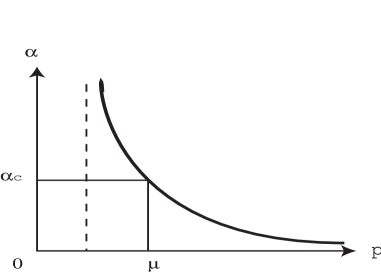
Fig. 6: The running coupling constant in the APEGT.

7 Reformulation of Yang-Mills theory

In this section we summarize the novel reformulation of the Yang-Mills theory proposed in Ref.? and elaborated in Ref.?. This material is necessary for subsequent sections.

7.1 Deformation of topological field theory

We consider the quantization of Yang-Mills theory on the topological background field. We decompose the connection ${\cal A}$ as

$${\cal A}_{\mu}(x)=\mathchar 28938\relax_{\mu}(x)+{\cal Q}_{\mu}(x)$$ (7.1)

and identify ${\cal Q}$ with the quantum fluctuation field on the background field $\mathchar 28938\relax$. For arbitrary but fixed background field $\mathchar 28938\relax$, the generating functional is given by

$$\tilde{Z}[J,\mathchar 28938\relax] := \int[d{\cal Q}][d\tilde{C}][d\bar{\tilde{C}}][d\tilde{B}]\exp\{iS_{YM}[\mathchar 28938\relax+{\cal Q}]$$ (7.2)

$$+i\tilde{S}_{GF}[Q,\tilde{C},\bar{\tilde{C}},\tilde{B}]+i(J_{\mu}\cdot{\cal Q}_{\mu})\},$$

where $S_{YM}[{\cal A}]$ is the usual Yang-Mills action,

$$S_{YM}[{\cal A}]=-\int d^{D}x{1\over 4}{\cal F}_{\mu\nu}^{A}[{\cal A}]{\cal F}^{\mu\nu}{}^{A}[{\cal A}],$$ (7.3)

and $\tilde{S}_{GF}$ is the gauge-fixing and FP ghost term for the quantum fluctuation field ${\cal Q}$:

$$\tilde{S}_{GF}[{\cal Q},\tilde{C},\bar{\tilde{C}},\tilde{B}] := -\int d^{D}x\ i\tilde{\delta}_{B}\ {\rm tr}_{G}\left[\bar{\tilde{C}}\left(\tilde{F}[{\cal Q}]+{\tilde{\alpha}\over 2}\tilde{B}\right)\right].$$ (7.4)

We wish to retain gauge invariance for the background field $\mathchar 28938\relax$ even after the gauge fixing for ${\cal Q}$. This is realized by choosing the background field (BGF) gauge fixing condition

$$\tilde{F}^{A}[{\cal Q}]:={\cal D}_{\mu}^{AB}[\mathchar 28938\relax]{\cal Q}^{\mu}{}^{B}=0.$$ (7.5)

In fact, in the BGF gauge, $\tilde{Z}[J,\mathchar 28938\relax]$ is invariant under the gauge transformation of the background field; the infinitesimal version is given by $\delta\mathchar 28938\relax_{\mu}={\cal D}_{\mu}[\mathchar 28938\relax]\omega.$ Hence, the theory with the action

$$\tilde{S}_{eff}[J,\mathchar 28938\relax]:=-i\ln\tilde{Z}[J,\mathchar 28938\relax],$$ (7.6)

is defined only on the space of the gauge orbit. Suppose that the background field satisfies the equation $F^{A}[\mathchar 28938\relax]=0.$ In order to consider the quantized Yang-Mills theory on all possible background fields satisfying the equations $F^{A}[\mathchar 28938\relax]=0,$ we define the total generating functional

$$Z[J]=\int[d\mathchar 28938\relax_{\mu}][dC][d\bar{C}][dB]\tilde{Z}[J,\mathchar 28938\relax]\exp(iS_{TQFT}[\mathchar 28938\relax,C,\bar{C},B])\exp[i(J_{\mu}\cdot\mathchar 28938\relax^{\mu})]$$ (7.7)

$$= \int[d\mathchar 28938\relax_{\mu}][dC][d\bar{C}][dB]\exp\{i\tilde{S}_{eff}[J,\mathchar 28938\relax]+iS_{TQFT}[\mathchar 28938\relax,C,\bar{C},B]+i(J_{\mu}\cdot\mathchar 28938\relax^{\mu})\},$$

where $S_{TQFT}[\mathchar 28938\relax,C,\bar{C},B]$ corresponds to the gauge-fixing term for the background field $\mathchar 28938\relax_{\mu}$. In order to describe the magnetic monopole as a topological background field in Yang-Mills theory, we choose the MA gauge for $\mathchar 28938\relax_{\mu}$,

$$S_{TQFT}[\mathchar 28938\relax,C,\bar{C},B] := -\int d^{D}x\ i\delta_{B}\ {\rm tr}_{G/H}\left[\bar{C}\left(F[\mathchar 28938\relax]+{\alpha\over 2}B\right)\right],$$ (7.8)

where

$$F^{a}[\mathchar 28938\relax]:=D_{\mu}{}^{ab}{}[\mathchar 28938\relax^{i}]\mathchar 28938\relax^{\mu}{}^{b}:=(\partial_{\mu}\delta^{ab}-gf^{abi}\mathchar 28938\relax_{\mu}{}^{i})\mathchar 28938\relax^{\mu}{}^{b}\quad(i=1,\cdots,N-1).$$ (7.9)

Note that the trace is taken on the coset $G/H$, not on the entire $G$, in the MA gauge.

Under the identification

$$\mathchar 28938\relax_{\mu}(x):={i\over g}U(x)\partial_{\mu}U^{\dagger}(x),\quad{\cal Q}_{\mu}(x):=U(x){\cal V}_{\mu}(x)U^{\dagger}(x),$$ (7.10)

we assume that all the topologically non-trivial configurations come from $\mathchar 28938\relax$, whereas ${\cal V}$ denotes topologically trivial configurations. Therefore, ${\cal V}$ changes under the small gauge transformation, while $\mathchar 28938\relax$ includes the effect of large gauge transformations. Therefore, we must take into account the finite gauge rotation $U$, without restriction to the infinitesimal gauge transformation. Under the identification (7.10), the Yang-Mills action is invariant,

$$S_{YM}[{\cal A}]=S_{YM}[\mathchar 28938\relax+{\cal Q}]=S_{YM}[{\cal V}]=\int d^{D}x{-1\over 4}{\cal F}_{\mu\nu}^{A}[{\cal V}]{\cal F}^{\mu\nu}{}^{A}[{\cal V}],$$ (7.11)

while the gauge-fixing term (7.4) is changed [17] into

$$\tilde{S}_{GF}[{\cal V},\gamma,\bar{\gamma},\beta] := -\int d^{D}x\ i\tilde{\delta}_{B}\ {\rm tr}_{G}\left[\bar{\gamma}\left(\partial^{\mu}{\cal V}_{\mu}+{\tilde{\alpha}\over 2}\beta\right)\right].$$ (7.12)

This implies that the background gauge for ${\cal Q}$ is changed into the Lorentz gauge for ${\cal V}$, $\partial_{\mu}{\cal V}_{\mu}=0$. Then the generating functional in the background field $\mathchar 28938\relax$ is cast into

$$\tilde{Z}[J,\mathchar 28938\relax]=\int[d{\cal V}][d\gamma][d\bar{\gamma}][d\beta]\exp\left\{iS_{YM}[{\cal V}]+i\tilde{S}_{GF}[{\cal V},\gamma,\bar{\gamma},\beta]+i(J_{\mu}\cdot U{\cal V}^{\mu}U^{\dagger})\right\},$$

where ${\cal V}_{\mu},\gamma,\bar{\gamma}$ and $\beta$ are defined by the adjoint rotations of ${\cal Q}_{\mu},\tilde{C},\bar{\tilde{C}}$ and $\bar{B}$ respectively:

$${\cal V}_{\mu}:=U^{\dagger}{\cal Q}_{\mu}U,\quad\gamma:=U^{\dagger}\tilde{C}U,\quad\bar{\gamma}:=U^{\dagger}\bar{\tilde{C}}U,\quad\beta:=U^{\dagger}\tilde{B}U.$$ (7.14)

Thus the total generating functional reads

$$Z[J]=\int[dU][dC][d\bar{C}][dB]\tilde{Z}[J,\mathchar 28938\relax]\exp(iS_{GF}[\mathchar 28938\relax,C,\bar{C},B])\exp[i(J_{\mu}\cdot\mathchar 28938\relax^{\mu})]$$

$$= \int[dU][dC][d\bar{C}][dB]\exp\{i\tilde{S}_{eff}[J,\mathchar 28938\relax]+iS_{TQFT}[\mathchar 28938\relax,C,\bar{C},B]+i(J_{\mu}\cdot\mathchar 28938\relax^{\mu})\},$$

where we have made a change of variable from $\mathchar 28938\relax$ to $U$. The measure $[dU]$ is invariant under the multiplication

$$U(x)\rightarrow\tilde{U}(x)U(x),$$ (7.16)

which leads to the finite gauge transformation of the background field,

$$\mathchar 28938\relax(x)\rightarrow\tilde{U}(x)\mathchar 28938\relax(x)\tilde{U}^{\dagger}(x)+{i\over g}\tilde{U}(x)d\tilde{U}^{\dagger}(x).$$ (7.17)

The modified MA gauge proposed in Ref.[13] leads to the TQFT with the action

$$S_{TQFT}[\mathchar 28938\relax,C,\bar{C},B]:=\int_{{\bf R}^{D}}d^{D}x\ i\delta_{B}\bar{\delta}_{B}{\rm tr}_{G/H}\left[{1\over 2}\mathchar 28938\relax_{\mu}\mathchar 28938\relax^{\mu}-{\alpha\over 2}iC\bar{C}\right].$$ (7.18)

The expectation value of the functional $f({\cal A})$ of ${\cal A}$ is calculated as follows. If the functional is of the form $f({\cal A})=g({\cal V}_{\mu},U)h(U)$, then the expectation value is calculated according to

$$\langle f({\cal A})\rangle_{YM}=\langle\langle g({\cal V}_{\mu},U)\rangle_{pYM}^{{\cal V}}h(U)\rangle_{TQFT}^{U},$$ (7.19)

where the sector of the perturbative deformation is defined by

$$\langle(\cdots)\rangle_{pYM}^{{\cal V}} = Z_{pYM}^{-1}\int[d{\cal V}][d\gamma][d\bar{\gamma}][d\beta]\exp\left\{iS_{YM}[{\cal V}]+i\tilde{S}_{GF}[{\cal V},\gamma,\bar{\gamma},\beta]\right\}(\cdots),$$

$$Z_{pYM} := \int[d{\cal V}][d\gamma][d\bar{\gamma}][d\beta]\exp\left\{iS_{YM}[{\cal V}]+i\tilde{S}_{GF}[{\cal V},\gamma,\bar{\gamma},\beta]\right\},$$ (7.20)

and the sector topological field theory is defined by

$$\langle(\cdots)\rangle_{TQFT}^{U} := Z_{TQFT}^{-1}\int[dU][dC][d\bar{C}][dB]\exp\{iS_{TQFT}[\mathchar 28938\relax,C,\bar{C},B]\}(\cdots),$$

$$Z_{TQFT} := \int[dU][dC][d\bar{C}][dB]\exp\{iS_{TQFT}[\mathchar 28938\relax,C,\bar{C},B]\}.$$ (7.21)

This reformulation of the Yang-Mills theory is called the “perturbative deformation of a topological quantum field theory”. The expectation value $\langle(\cdots)\rangle_{pYM}^{{\cal V}}$ for the field ${\cal V}$ is calculated using a perturbation theory in terms of the coupling constant $g$. On the other hand, the expectation value $\langle(\cdots)\rangle_{TQFT}^{U}$ should be calculated in a non-perturbative way to incorporate the topological contribution. Here $U$ is a compact gauge variable corresponding to a finite gauge transformation. In the instanton calculus, the integration measure $[dU]$ is replaced with the (finite-dimensional) integration over the collective coordinates of the instanton.

7.2 Dimensional reduction to the NLS model in the MA gauge

It has been shown [13] that, due to the hidden supersymmetry $OSp(D|2)$, the TQFT part (7.18) is reduced to the $(D-2)$-dimensional coset ($G/H$) nonlinear sigma (NLS) model,

$$S_{NLSM}[U,C,\bar{C}]:=\alpha\pi\int_{{\bf R}^{D-2}}d^{D-2}x\ {\rm tr}_{G/H}\left[{1\over 2}\mathchar 28938\relax_{\mu}\mathchar 28938\relax_{\mu}-{\alpha\over 2}iC\bar{C}\right],$$ (7.22)

where, for the matrix element $\mathchar 28938\relax_{ab}$ (see Appendix C),

$${\rm tr}_{G/H}\left[{1\over 2}\mathchar 28938\relax_{\mu}(x)\mathchar 28938\relax_{\mu}(x)\right]=\sum_{a,b:a<b}(\mathchar 28938\relax_{\mu}(x))_{ab}(\mathchar 28938\relax_{\mu}(x))_{ab}.$$ (7.23)

By making use of the complex coordinates in the flag space $G/H$, the action can be rewritten as (see Appendix C)

$$S_{NLSM} = {\alpha\pi\over 2g^{2}}\int_{{\bf R}^{D-2}}d^{D-2}xg_{\alpha\bar{\beta}}{\partial w^{\alpha}\over\partial x_{a}}{\partial\bar{w}^{\beta}\over\partial x_{a}},\quad(a=1,\cdots,D-2)$$ (7.24)

where we have omitted to write the decoupled ghost term, $C(x)\bar{C}(x)$. In particular, for $D=4$,

$$S_{NLSM}={\alpha\pi\over 2g^{2}}\int_{{\bf C}}dzd\bar{z}\ g_{\alpha\bar{\beta}}\left({\partial w^{\alpha}\over\partial z}{\partial\bar{w}^{\beta}\over\partial\bar{z}}+{\partial w^{\alpha}\over\partial\bar{z}}{\partial\bar{w}^{\beta}\over\partial z}\right),$$ (7.25)

where $z=x+iy=x_{1}+ix_{2}\in{\bf C}\cong{\bf R}^{2}$ and $dxdy=dx_{1}dx_{2}={i\over 2}dzd\bar{z}$. The $G=SU(2)$ case is analyzed in Ref.?, and in that case we have

$$S_{NLSM}={\alpha\pi\over 2g^{2}}\int_{{\bf C}}dzd\bar{z}\ {1\over(1+|w|^{2})^{2}}\left({\partial w\over\partial z}{\partial\bar{w}\over\partial\bar{z}}+{\partial w\over\partial\bar{z}}{\partial\bar{w}\over\partial z}\right).$$ (7.26)

The above described strategy is schematically depicted below.

8 Area law of the Wilson loop (I)

In this section we derive the area law of the Wilson loop based on the instanton calculus. ?, ?, ? A more systematic estimation is given in the next section based on the large $N$ expansion.

The static potential $V(R)$ is evaluated from the rectangular Wilson loop $C$ with sides $T$ and $R$ according to

$$V(R):=-\lim_{T\rightarrow\infty}{1\over T}\ln\langle W^{C}[{\cal A}]\rangle_{YM_{4}}.$$ (8.1)

The (full) string tension $\sigma$ is defined by

$$\sigma:=-\lim_{A(C)\rightarrow\infty}{1\over A(C)}\ln\langle W^{C}[{\cal A}]\rangle_{YM_{4}},$$ (8.2)

where $A(C)$ is the minimal area of the surface spanned by the Wilson loop $C$. Of course, the rectangular loop has minimal area: $A(C)=TR$.

Using the NAST for the Wilson loop operator,

$$W^{C}[{\cal A}]=\int[d\mu(\xi)]_{C}\exp\left(ig\oint_{C}n^{A}{\cal A}^{A}+i\oint_{C}\omega\right),$$ (8.3)

we can write its expectation value in the Yang-Mills theory as [15, 17]

$$\langle W^{C}[{\cal A}]\rangle_{YM_{4}}$$ (8.4)

$$= \Biggr{\langle}\Biggr{\langle}\exp\left[ig\oint_{C}dx^{\mu}n^{A}(x){\cal V}_{\mu}^{A}(x)\right]\Biggr{\rangle}_{pYM_{4}}\exp\left[i\oint_{C}\omega\right]\Biggr{\rangle}_{TQFT_{4}},$$

where the measure $\int[d\mu(\xi)]_{C}$ gives a redundant factor which does not affect the string tension in the area law, as shown in Section IV.C of Ref. ? and hence it is omitted in the following.

8.1 Perturbative expansion and dimensional reduction

In our reformulation, the field ${\cal V}_{\mu}^{A}(x)$ is identified with the perturbative deformation. Thus we expand the first exponential of (8.4) in powers of the coupling constant $g$:

$$\Biggr{\langle}\exp\left[ig\oint_{C}dx^{\mu}n^{A}(x){\cal V}_{\mu}^{A}(x)\right]\Biggr{\rangle}_{pYM_{4}}$$ (8.5)

$$= 1+\sum_{n=1}^{\infty}{(ig)^{n}\over n!}\oint_{C}dx_{1}^{\mu_{1}}\oint_{C}dx_{2}^{\mu_{2}}\cdots\oint_{C}dx_{n}^{\mu_{n}}n^{A_{1}}(x_{1})n^{A_{2}}(x_{2})\cdots n^{A_{n}}(x_{n})$$

$$\times\langle{\cal V}_{\mu_{1}}^{A_{1}}(x_{1}){\cal V}_{\mu_{2}}^{A_{2}}(x_{2})\cdots{\cal V}_{\mu_{n}}^{A_{n}}(x_{n})\rangle_{pYM_{4}}.$$

Hence, we obtain

$$\langle W^{C}[{\cal A}]\rangle_{YM_{4}}$$ (8.7)

$$=\Biggr{\langle}\exp\left[i\oint_{C}\omega\right]\Biggr{\rangle}_{TQFT_{4}}+\sum_{n=1}^{\infty}{(ig)^{n}\over n!}\oint_{C}dx_{1}^{\mu_{1}}\oint_{C}dx_{2}^{\mu_{2}}\cdots\oint_{C}dx_{n}^{\mu_{n}}$$

$$\times\Biggr{\langle}n^{A_{1}}(x_{1})n^{A_{2}}(x_{2})\cdots n^{A_{n}}(x_{n})\exp\left[i\oint_{C}\omega\right]\Biggr{\rangle}_{TQFT_{4}}$$

$$\times\langle{\cal V}_{\mu_{1}}^{A_{1}}(x_{1}){\cal V}_{\mu_{2}}^{A_{2}}(x_{2})\cdots{\cal V}_{\mu_{n}}^{A_{n}}(x_{n})\rangle_{pYM_{4}}.$$

$$= \Biggr{\langle}\exp\left[i\oint_{C}\omega\right]\Biggr{\rangle}_{TQFT_{4}}$$

$$\times\Biggr{[}1+\sum_{n=1}^{\infty}{(ig)^{n}\over n!}\oint_{C}dx_{1}^{\mu_{1}}\oint_{C}dx_{2}^{\mu_{2}}\cdots\oint dx_{n}^{\mu_{n}}\langle{\cal V}_{\mu_{1}}^{A_{1}}(x_{1}){\cal V}_{\mu_{2}}^{A_{2}}(x_{2})\cdots{\cal V}_{\mu_{n}}^{A_{n}}(x_{n})\rangle_{pYM_{4}}$$

$$\times{\langle n^{A_{1}}(x_{1})n^{A_{2}}(x_{2})\cdots n^{A_{n}}(x_{n})\exp\left[i\oint_{C}\omega\right]\rangle_{TQFT_{4}}\over\langle\exp\left[i\oint_{C}\omega\right]\rangle_{TQFT_{4}}}\Biggr{]}.$$

We restrict the Wilson loop to a planar loop. This choice has the following advantage. For the planar Wilson loop $C$, the Parisi-Sourlas dimensional reduction leads to the following identities:[13]

$${\hbox{$\left\langle\vbox to0.0pt{}\right.\n@space$}}\exp\left[i\oint_{C}\omega\right]{\hbox{$\left\rangle\vbox to0.0pt{}\right.\n@space$}}_{TQFT_{4}}={\hbox{$\left\langle\vbox to0.0pt{}\right.\n@space$}}\exp\left[i\oint_{C}\omega\right]{\hbox{$\left\rangle\vbox to0.0pt{}\right.\n@space$}}_{NLSM_{2}},$$ (8.8)

and

$$\Biggr{\langle}n^{A_{1}}(x_{1})\cdots n^{A_{n}}(x_{n})\exp\left[i\oint_{C}\omega\right]\Biggr{\rangle}_{TQFT_{4}}=\Biggr{\langle}n^{A_{1}}(x_{1})\cdots n^{A_{n}}(x_{n})\exp\left[i\oint_{C}\omega\right]\Biggr{\rangle}_{NLSM_{2}},$$ (8.9)

where $x_{1},\cdots,x_{n}\in C\subset{\bf R}^{2}$. This is because, in the case of the fundamental representation of $SU(N)$, $n^{A}$ and $\omega$ can be written in terms of $U$ as (see (4.28), (4.29))

$$n^{A}(x) = U_{1a}(x)(T^{A})_{ab}\bar{U}_{1b}(x)=\bar{\phi}_{a}(x)(T^{A})_{ab}\phi_{b}(x),$$ (8.10)

$$\omega(x) = {i\over 2}[U_{1a}(x)d\bar{U}_{1a}(x)-dU_{1a}(x)\bar{U}_{1a}(x)]$$ (8.11)

$$= {i\over 2}[\bar{\phi}_{a}(x)d\phi_{a}(x)-d\bar{\phi}_{a}(x)\phi_{a}(x)].$$

Taking the logarithm of the Wilson loop (8.7) and expanding it in powers of the coupling constant, we obtain

$$\ln\langle W^{C}[{\cal A}]\rangle_{YM_{4}}$$ (8.13)

$$= \ln\Biggr{\langle}\exp\left[i\oint_{C}\omega\right]\Biggr{\rangle}_{NLSM_{2}}$$

$$+\ln\left[1-{g^{2}\over 2}\oint_{C}dx^{\mu}\oint_{C}dy^{\nu}G_{\mu\nu}^{AB}(x,y){\langle n^{A}(x)n^{B}(y)\exp\left[i\int_{S}\mathchar 28938\relax_{K}\right]\rangle_{NLSM_{2}}\over\langle\exp\left[i\oint_{C}\omega\right]\rangle_{NLSM_{2}}}+O(g^{4})\right]$$

$$= \ln\Biggr{\langle}\exp\left[i\oint_{C}\omega\right]\Biggr{\rangle}_{NLSM_{2}}$$

$$-{g^{2}\over 2}\oint_{C}dx^{\mu}\oint_{C}dy^{\nu}G_{\mu\nu}^{AB}(x,y){\langle n^{A}(x)n^{B}(y)\exp\left[i\oint_{C}\omega\right]\rangle_{NLSM_{2}}\over\langle\exp\left[i\oint_{C}\omega\right]\rangle_{NLSM_{2}}}+O(g^{4}),$$

where we have defined the two-point function

$$G_{\mu\nu}^{AB}(x,y):=\langle{\cal V}_{\mu}^{A}(x){\cal V}_{\nu}^{B}(y)\rangle_{pYM_{4}}.$$ (8.14)

In the rest of this section we focus on the first term in (8.13). The remaining terms will be estimated in the next section.

8.2 The instanton in $F_{N-1}$ and $CP^{N-1}$ models

We wish to demonstrate the area law for the expectation value,

$${\hbox{$\left\langle\vbox to0.0pt{}\right.\n@space$}}\exp\left(i\oint_{C}\omega\right){\hbox{$\left\rangle\vbox to0.0pt{}\right.\n@space$}}_{NLSM_{2}}\equiv{\hbox{$\left\langle\vbox to0.0pt{}\right.\n@space$}}\exp\left(i\int_{S}\mathchar 28938\relax_{K}\right){\hbox{$\left\rangle\vbox to0.0pt{}\right.\n@space$}}_{NLSM_{2}}$$ (8.15)

$$= Z_{NLSM_{2}}^{-1}\int[d\mu(w,\bar{w})]\exp(-S_{NLSM_{2}}[w,\bar{w}])\exp\left(i\int_{S}\mathchar 28938\relax_{K}\right),$$ (8.16)

where the two-dimensional NLS model is defined by the action

$$S_{NLSM_{2}} = {\pi\over g^{2}(\mu)}\int_{{\bf R}^{2}}d^{2}xg_{\alpha\bar{\beta}}{\partial w^{\alpha}\over\partial x_{a}}{\partial\bar{w}^{\beta}\over\partial x_{a}}$$ (8.17)

$$= {\pi\over g^{2}(\mu)}\int_{{\bf C}}dzd\bar{z}\ g_{\alpha\bar{\beta}}\left({\partial w^{\alpha}\over\partial z}{\partial\bar{w}^{\beta}\over\partial\bar{z}}+{\partial w^{\alpha}\over\partial\bar{z}}{\partial\bar{w}^{\beta}\over\partial z}\right),$$ (8.18)

where

$$z=x+iy=x_{1}+ix_{2}\in{\bf C}\cong{\bf R}^{2},\quad dxdy=dx_{1}dx_{2}={i\over 2}dzd\bar{z},$$ (8.19)

and $g(\mu)$ is the Yang-Mills coupling constant.

Note that the action satisfies the inequality,

$$S_{NLSM} = {\pi\over 2g^{2}(\mu)}\int_{{\bf R}^{2}}d^{2}xg_{\alpha\bar{\beta}}(\partial_{a}w^{\alpha}\pm i\epsilon_{ab}\partial_{b}w^{\alpha})(\partial_{a}w^{\beta}\pm i\epsilon_{ac}\partial_{c}w^{\beta})^{*}$$ (8.21)

$$\pm i{\pi\over g^{2}(\mu)}\int_{{\bf R}^{2}}d^{2}x\epsilon_{ab}g_{\alpha\bar{\beta}}{\partial w^{\alpha}\over\partial x_{a}}{\partial\bar{w}^{\beta}\over\partial x_{b}}$$

$$\geq\pm i{\pi\over g^{2}(\mu)}\int_{{\bf R}^{2}}d^{2}x\epsilon_{ab}g_{\alpha\bar{\beta}}{\partial w^{\alpha}\over\partial x_{a}}{\partial\bar{w}^{\beta}\over\partial x_{b}}.$$

This inequality is saturated when $w^{\alpha}$ satisfies the equation $\partial_{a}w^{\alpha}\pm i\epsilon_{ab}\partial_{b}w^{\alpha}=0,$ which is equivalent to the Cauchy-Riemann equation,

$$\bar{\partial}_{z}w^{\alpha}:=(\partial_{1}+i\partial_{2})w^{\alpha}=0.$$ (8.22)

The solution $w^{\alpha}=f^{\alpha}(z)$ is an arbitrary rational function of $z$.

The finite action configuration of the coset NLS model is provided by the instanton solution, which is a solution of the Cauchy-Riemann equation (8.22). It is known [23] that the integer-valued topological charge $Q$ of the instanton in the $F_{N-1}$ NLS model is given by the integral of the Kähler 2-form over ${\bf R}^{2}$:

$$Q={1\over\pi}\int\mathchar 28938\relax_{K} = \int_{{\bf R}^{2}}{d^{2}x\over\pi}\epsilon_{ab}g_{\alpha\bar{\beta}}{\partial w^{\alpha}\over\partial x_{a}}{\partial\bar{w}^{\beta}\over\partial x_{b}}$$ (8.23)

$$= \int_{{\bf C}}{dzd\bar{z}\over\pi}\ g_{\alpha\bar{\beta}}\left({\partial w^{\alpha}\over\partial z}{\partial\bar{w}^{\beta}\over\partial\bar{z}}-{\partial w^{\alpha}\over\partial\bar{z}}{\partial\bar{w}^{\beta}\over\partial z}\right).$$

This is a generalization of the $F_{1}$ case ($N=2$), where

$$Q={i\over 2\pi}\int_{{\bf C}}{dwd\bar{w}\over(1+|w|^{2})^{2}}={i\over 2\pi}\int_{S^{2}}{dzd\bar{z}\over(1+|w|^{2})^{2}}\left({\partial w\over\partial z}{\partial\bar{w}\over\partial\bar{z}}-{\partial w\over\partial\bar{z}}{\partial\bar{w}\over\partial z}\right).$$ (8.24)

Thus the instanton solution is characterized by the integral topological charge $Q\in{\bf Z}$. For instanton ($Q>0$) and anti-instanton ($Q<0$) configurations with a topological charge $Q$, the action has

$$S_{NLSM}={\pi^{2}\over g^{2}}|Q|.$$ (8.25)

The metric in the Kähler manifold $F_{N-1}$ is obtained in accordance with the relation $g_{\alpha\bar{\beta}}={\partial\over\partial w^{\alpha}}{\partial\over\partial\bar{w}^{\beta}}K$ from the Kähler potential,

$$K(w,\bar{w})=\sum_{\ell=1}^{N-1}d_{\ell}K_{\ell}(w,\bar{w})=\sum_{\ell=1}^{N-1}d_{\ell}\ln\mathchar 28929\relax_{\ell}(w,\bar{w}),$$ (8.26)

with the Dynkin indices $d_{\ell}(\ell=1,\cdots,N-1)$. Then the integral $\int\mathchar 28938\relax_{K}$ over the whole two-dimensional space reads

$$\int_{{\bf R}^{2}}\mathchar 28938\relax_{K}=\pi Q=\pi\sum_{\ell=1}^{N-1}d_{\ell}Q_{\ell},$$ (8.27)

where $Q_{\ell}$ are integer-valued topological charges. Hence, $\mathchar 28938\relax_{K}(x)/\pi$ is identified with the density of the topological charge (up to the weight due to the index $d_{\ell}$).

Now we consider the $CP^{N-1}$ model. If we identify $w_{\alpha}$ with the inhomogeneous coordinates, e.g., $w_{\alpha}:={\phi_{\alpha}\over\phi_{N}},$ the metric (3.63) can be rewritten as

$$g_{\alpha\bar{\beta}}(\phi)={(||\phi||^{2})\delta_{\alpha\beta}-\bar{\phi}_{\alpha}\phi_{\beta}\over(||\phi||^{2})^{2}},$$ (8.28)

where

$$||\phi||^{2}:=\sum_{\alpha=1}^{N}|\phi_{\alpha}|^{2}=|\phi_{N}|^{2}\left(1+|||w|||^{2}\right).$$ (8.29)

The action of the $CP^{N-1}$ model is given by

$$S_{CP^{N-1}}={\pi\over g^{2}}\int d^{d}xg_{\alpha\bar{\beta}}(w)\partial_{\mu}w^{\alpha}\partial_{\mu}\bar{w}^{\beta},$$ (8.30)

or equivalently,

$$S_{CP^{N-1}}={\pi\over g^{2}}\int d^{d}xg_{\alpha\bar{\beta}}(\phi)\partial_{\mu}\phi^{\alpha}\partial_{\mu}\bar{\phi}^{\beta}.$$ (8.31)

Under the constraint $||\phi||^{2}=1,$ the action can be written as

$$S_{CP^{N-1}} = {\beta_{g}\over 2}\int d^{d}x(\delta_{\alpha\beta}-\bar{\phi}_{\alpha}\phi_{\beta})\partial_{\mu}\phi^{\alpha}\partial_{\mu}\bar{\phi}^{\beta}$$ (8.32)

$$= {\beta_{g}\over 2}\int d^{d}x[(\partial_{\mu}\bar{\phi}^{\alpha}\partial_{\mu}\phi^{\alpha}+(\bar{\phi}^{\alpha}\partial_{\mu}\phi^{\alpha})(\bar{\phi}^{\beta}\partial_{\mu}\phi^{\beta})].$$

This agrees with the action of the $CP^{N-1}$ model presented in Ref.?. (See Appendix C for more details).

8.3 Area law in the dilute instanton-gas approximation

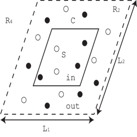
Fig. 7: Instanton and anti-instanton configuration and the Wilson loop $C$ in a finite-volume region $L_{1}\times L_{2}$ in the two-dimensional plane ${\bf R}^{2}$ embedded in ${\bf R}^{4}$.

If the Wilson loop is large compared with the typical size of the instanton, $\int_{S}\mathchar 28938\relax_{K}(x)/\pi$ in (8.16) counts the number of instantons $n_{+}^{in}$ minus anti-instantons $n_{-}^{in}$ that are contained inside the area $S\subset{\bf R}^{2}$ bounded by the loop $C$:

$$\int_{S}\mathchar 28938\relax_{K}=\pi(n_{+}^{in}-n_{-}^{in}).$$ (8.33)

(See Fig.7.) Thus, the expectation value $\langle\exp\left(i\int_{S}\mathchar 28938\relax_{K}\right)\rangle_{NLSM}$ is calculated by summing over all the possible cases of instanton and anti-instanton configurations (i.e., by the integration over the instanton moduli). In this calculation, we use

$$S_{NLSM}={\pi^{2}\over g^{2}}|Q|={\pi^{2}\over g^{2}}(n_{+}+n_{-}),\quad n_{\pm}=n_{\pm}^{in}+n_{\pm}^{out}.$$ (8.34)

where $n_{+}^{out}$ ($n_{-}^{out}$) is the number of instantons (anti-instantons) outside $S$, and $n_{+}$ ($n_{-}$) is the total number of instantons (anti-instantons). For the quark in the fundamental representation ${\bf N}$ ($d_{1}=1,d_{2}=d_{3}=\cdots=d_{N-1}=0$), this is easily carried out as follows.

For the $SU(3)$ case with $[1,0]$, an element $\xi\in F_{2}$ is independent of $w_{3}$, so that $w_{3}$ is redundant in this case. Hence, it suffices to consider the $CP^{2}$ model for the fundamental quark (up to Weyl symmetry). For $CP^{2}$, the Kähler two-form is given by (4.87)

$$\mathchar 28938\relax_{K} = im(\mathchar 28929\relax_{1})^{-2}[(1+|w_{1}|^{2})dw_{2}\wedge d\bar{w}_{2}-\bar{w}_{2}w_{1}dw_{2}\wedge d\bar{w}_{1}$$ (8.35)

$$-w_{2}\bar{w}_{1}dw_{1}\wedge d\bar{w}_{2}+(1+|w_{2}|^{2})dw_{1}\wedge d\bar{w}_{1}].$$

When $w_{2}=0$, $\mathchar 28938\relax_{K}$ reduces to

$$\mathchar 28938\relax_{K}=i(1+|w_{1}|^{2})^{-2}dw_{1}\wedge d\bar{w}_{1}.$$ (8.36)

Similarly, when $w_{1}=0$, we have

$$\mathchar 28938\relax_{K}=i(1+|w_{2}|^{2})^{-2}dw_{2}\wedge d\bar{w}_{2}.$$ (8.37)

For a polynomial $w_{\alpha}=w_{\alpha}(z)$ in $z=x+iy$ of order $n$, we find the instanton charge

$$\int\mathchar 28938\relax_{K}=\pi Q,\quad Q\in{\bf Z}.$$ (8.38)

This is the same situation as that encountered in $SU(2)$, in which case

$$\int\mathchar 28938\relax_{K}=2j\pi Q,$$ (8.39)

where $j=1/2$ corresponds to the fundamental representation.[13, 15] Thus the Wilson loop can be estimated by the naive instanton calculus. In fact, the dilute instanton gas approximation leads to the area law for the Wilson loop (see Ref.?). Here the factor $\pi$ is very important. The integral of the Kähler two-form $\mathchar 28938\relax_{K}$ is a multiple of $\pi$. If we had a factor $2\pi$, the area law would not hold, just as in the $j=1$ case of $SU(2)$.

For the $SU(N)$ case with Dynkin index, $[1,0,\cdots,0]$, it suffices to consider the $CP^{N-1}$ model. When $w_{a}\not=0$ and $w_{b}=0$ for all $b\not=a$, the Kähler two-form (4.53) for $CP^{N-1}$ reduces to

$$\mathchar 28938\relax_{K}=i(1+|w_{a}|^{2})^{-2}dw_{a}\wedge d\bar{w}_{a},$$ (8.40)

with no summation over $a$. Therefore the above argument can be applied to $SU(N)$ for any $N$. This implies the confinement of fundamental quarks in $SU(N)$ Yang-Mills theory within the approximation of a dilute instanton gas. This naive instanton calculation can be improved by including fluctuations from the instanton solutions following Ref.?, and this issue will be discussed in detail in a subsequent article.[43]

9 Area law of the Wilson loop (II)

The derivation of the area law of the Wilson loop in the four-dimensional Yang-Mills theory in the MA gauge is reduced to demonstrating the area law of the diagonal Wilson loop in the two-dimensional coset NLS model. In this section we complete a derivation of the area law of the Wilson loop in the fundamental representation. Here we use the large $N$ expansion [56, 57, 58, 59, 60] for the coset NLS model. (See, e.g., Refa.?, ?, ?, ? for reviews of the large $N$ expansion.)

To perform the large N expansion, it is convenient to introduce the new variables

$$P_{ab}(x) := \bar{\phi}_{a}(x)\phi_{b}(x)=U_{1a}(x)\bar{U}_{1b}(x),$$ (9.1)

$${\cal V}_{\mu}^{ab}(x) := {\cal V}_{\mu}^{A}(x)(T^{A})_{ab},$$ (9.2)

which are used to rewrite

$$C_{\mu}(x):=n^{A}(x){\cal V}_{\mu}^{A}(x)=P_{ab}(x){\cal V}_{\mu}^{ab}(x),$$ (9.3)

where $A=1,\cdots,N^{2}-1$ and $a,b=1,\cdots N$ for $SU(N)$.

In terms of the above variables, the expansion (8.7) of the expectation value of the Wilson loop operator in powers of the coupling constant $g$ is rewritten as

$$\langle W^{C}[{\cal A}]\rangle_{YM_{4}} = \Biggr{\langle}\exp\left[i\oint_{C}\omega\right]\Biggr{\rangle}_{TQFT_{4}}+\sum_{n=1}^{\infty}{(ig)^{n}\over n!}\oint_{C}dx_{1}^{\mu_{1}}\oint_{C}dx_{2}^{\mu_{2}}\cdots\oint_{C}dx_{n}^{\mu_{n}}$$ (9.5)

$$\times\langle{\cal V}_{\mu_{1}}^{a_{1}b_{1}}(x_{1}){\cal V}_{\mu_{2}}^{a_{2}b_{2}}(x_{2})\cdots{\cal V}_{\mu_{n}}^{a_{n}b_{n}}(x_{n})\rangle_{pYM_{4}}$$

$$\times\Biggr{\langle}P_{a_{1}b_{1}}(x_{1})P_{a_{2}b_{2}}(x_{2})\cdots P_{a_{n}b_{n}}(x_{n})\exp\left[i\oint_{C}\omega\right]\Biggr{\rangle}_{TQFT_{4}}$$

$$= \Biggr{\langle}\exp\left[i\oint_{C}\omega\right]\Biggr{\rangle}_{TQFT_{4}}$$

$$\times\Biggr{[}1+\sum_{n=1}^{\infty}{(ig)^{n}\over n!}\oint_{C}dx_{1}^{\mu_{1}}\oint_{C}dx_{2}^{\mu_{2}}\cdots\oint_{C}dx_{n}^{\mu_{n}}$$

$$\times\langle{\cal V}_{\mu_{1}}^{a_{1}b_{1}}(x_{1}){\cal V}_{\mu_{2}}^{a_{2}b_{2}}(x_{2})\cdots{\cal V}_{\mu_{n}}^{a_{n}b_{n}}(x_{n})\rangle_{pYM_{4}}$$

$$\times{\langle P_{a_{1}b_{1}}(x_{1})P_{a_{2}b_{2}}(x_{2})\cdots P_{a_{n}b_{n}}(x_{n})\exp\left[i\oint_{C}\omega\right]\rangle_{TQFT_{4}}\over\langle\exp\left[i\oint_{C}\omega\right]\rangle_{TQFT_{4}}}\Biggr{]}.$$

The diagrams needed to calculate this expectation value are drawn in Fig.9 based on the Feynmann rule given in Fig.8. Here it should be remarked that the definition of the Wilson loop operator

$$\langle W^{C}[{\cal A}]\rangle:={1\over{\cal N}}\Biggr{\langle}{\rm tr}\left[{\cal P}\exp\left(ig\oint_{C}dx^{\mu}{\cal A}_{\mu}(x)\right)\right]\Biggr{\rangle}_{YM_{4}},$$ (9.6)

includes the normalization factor ${\cal N}^{-1}$ and that the expectation value (9.6) of the Wilson loop may have a well-defined large $N$ limit. In particular, in the zero coupling limit, the expectation value reduces to one.

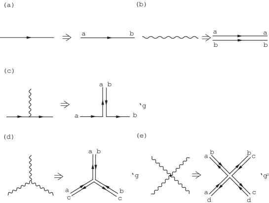
Fig. 8: Feynmann rule and the corresponding large $N$ rule (double line notation due to ’t Hooft) in QCD. Propagators: (a) quark propagator, (b) gluon propagator. Vertices: (c) quark-gluon vertex ($g_{YM}$), (d) three-gluon vertex ($g_{YM}$), (e) four-gluon vertex ($g_{YM}^{2}$).

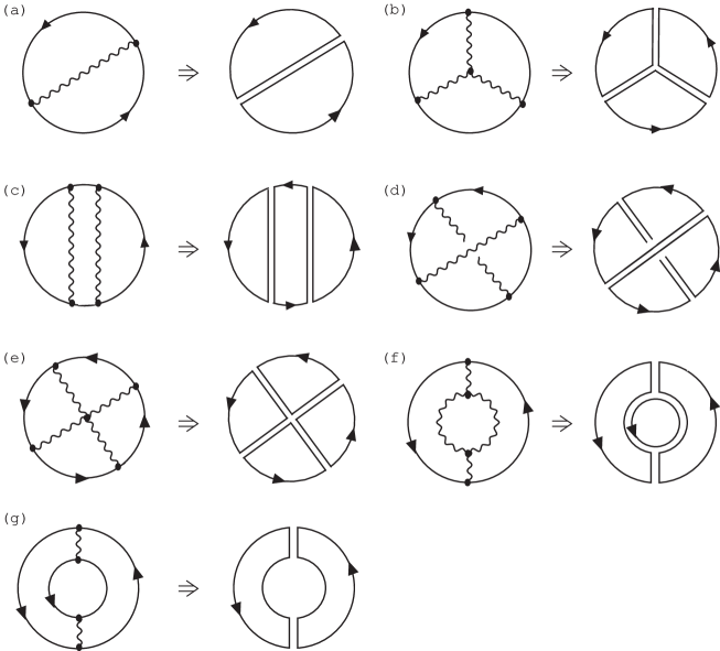
Fig. 9: Examples of Feynmann diagrams and the corresponding double line notations that appear in calculating the expectation value of the Wilson loop operator. The order of each diagram is estimated using the rule given in Fig. 8 as (a) $g_{YM}^{2}N^{2}=\lambda N$, (b) $g_{YM}^{4}N^{3}=\lambda^{2}N$, (c) $g_{YM}^{4}N^{3}=\lambda^{2}N$, (d) $g_{YM}^{4}N=\lambda^{2}/N$, (e) $g_{YM}^{6}N^{4}=\lambda^{3}N$, (f) $g_{YM}^{4}N^{3}=\lambda^{2}N$, and (g) $g_{YM}^{4}N^{2}=\lambda^{2}N^{0}$. [Here note that each contribution should be divided by the normalization factor $N$ for the fundamental quark, in agreement with the definition (9.6).] In the leading order of large $N$ expansion, the leading contributions come from the planar diagrams, e.g., (a), (b), (c), (e) and (f), which are furthermore classified by the order of $\lambda$. Note that the contribution from a nonplanar diagram (d) is suppressed for large $N$. The diagram (g) is the vacuum polarization diagram due to quark–anti-quark pair creation and annihilation, which is neglected in the pure Yang-Mills theory without dynamical quarks.

9.1 Large N expansion and dimensional reduction

It is known [32] that only the planar diagrams contribute to the expectation value

$$\langle{\cal A}_{\mu_{1}}^{a_{1}b_{1}}(x_{1}){\cal A}_{\mu_{2}}^{a_{2}b_{2}}(x_{2})\cdots{\cal A}_{\mu_{n}}^{a_{n}b_{n}}(x_{n})\rangle_{YM_{4}}$$ (9.7)

in the leading order of the large $N$ expansion. See Fig. 9. However, it is extremely difficult to sum up the infinite number of terms belonging to the leading order of the large $N$ expansion and to obtain a closed expression in the four-dimensional case. Of course, this does not exclude the possibility that the closed expression obtained by summing up all the leading diagrams may exhibit the area law. In fact, this strategy has been applied in the two-dimensional case and has successfully lead to the area law (see, e.g., Ref.?).

For the planar Wilson loop $C$, we have already shown that the Parisi-Sourlas dimensional reduction occurs and that the TQFT sector reduces to the two-dimensional coset NLS model, i.e. the NLS model on the flag space $F_{N-1}$. Hence, we obtain

$${\hbox{$\left\langle\vbox to0.0pt{}\right.\n@space$}}e^{i\oint_{C}\omega}{\hbox{$\left\rangle\vbox to0.0pt{}\right.\n@space$}}_{TQFT_{4}}={\hbox{$\left\langle\vbox to0.0pt{}\right.\n@space$}}e^{i\oint_{C}\omega}{\hbox{$\left\rangle\vbox to0.0pt{}\right.\n@space$}}_{NLSM_{2}},$$ (9.8)

and

$$\Biggr{\langle}P_{a_{1}b_{1}}(x_{1})\cdots P_{a_{n}b_{n}}(x_{n})e^{i\oint_{C}\omega}\Biggr{\rangle}_{TQFT_{4}}=\Biggr{\langle}P_{a_{1}b_{1}}(x_{1})\cdots P_{a_{n}b_{n}}(x_{n})e^{i\oint_{C}\omega}\Biggr{\rangle}_{NLSM_{2}},$$ (9.9)

where $x_{1},\cdots,x_{n}\in C\subset{\bf R}^{2}$. For the quark in the fundamental representation of $SU(N)$, the relevant NLS model can be restricted to the $CP^{N-1}$ model.

We now return to the expression (9.5) obtained by way of the NAST and apply the large $N$ expansion to the (perturbative) deformation sector and the TQFT sector simultaneously. Taking the logarithm of the Wilson loop, therefore, we obtain

$$\ln\langle W^{C}[{\cal A}]\rangle_{YM_{4}}$$ (9.10)

$$= \ln\Biggr{\langle}\exp\left[i\oint_{C}\omega\right]\Biggr{\rangle}_{CP^{N-1}_{2}}+\ln\left[1-f[C]+O(\lambda^{2}/N^{2})\right]$$

$$= \ln\Biggr{\langle}\exp\left[i\oint_{C}\omega\right]\Biggr{\rangle}_{CP^{N-1}_{2}}-f[C]+O(\lambda^{2}/N^{2}),$$

where we have defined the two-point correlation function

$$G_{\mu\nu}^{ab,cd}(x,y) := \langle{\cal V}_{\mu}^{ab}(x){\cal V}_{\nu}^{cd}(y)\rangle_{pYM_{4}},$$ (9.11)

and

$$f[C]:={g^{2}\over 2}\oint_{C}dx^{\mu}\oint_{C}dy^{\nu}G_{\mu\nu}^{ab,cd}(x,y){\langle P_{ab}(x)P_{cd}(y)\exp\left[i\oint_{C}\omega\right]\rangle_{CP^{N-1}_{2}}\over\langle\exp\left[i\oint_{C}\omega\right]\rangle_{CP^{N-1}_{2}}}.$$ (9.12)

It should be remarked that the $f[C]$ is $O(\lambda/N)$. This is different from the result of the usual large $N$ expansion of the Yang-Mills theory, i.e., diagram (a) of Fig. 9, which is $O(\lambda)$. This fact is shown as follows. In a previous article,[17] it is shown that the perturbative sector obeys the Lorentz-type gauge fixing, $\partial_{\mu}{\cal V}_{\mu}=0,$ by virtue of the background gauge. Here we adopt the Feynman gauge to simplify the calculation. Then the propagator for ${\cal V}_{\mu}^{A}$ reads

$$\langle{\cal V}_{\mu}^{A}(x){\cal V}_{\nu}^{B}(y)\rangle_{pYM_{4}}=\delta^{AB}\delta_{\mu\nu}D(x,y),\quad D(x,y):={1\over 4\pi^{2}}{1\over|x-y|^{2}}.$$ (9.13)

Then we find

$$G_{\mu\nu}^{ab,cd}(x,y) := \langle{\cal V}_{\mu}^{ab}(x){\cal V}_{\nu}^{cd}(y)\rangle_{pYM_{4}}$$ (9.14)

$$= \langle{\cal V}_{\mu}^{A}(x){\cal V}_{\nu}^{B}(y)\rangle_{pYM_{4}}(T^{A})_{ab}(T^{B})_{cd}$$ (9.15)

$$= \delta_{\mu\nu}D(x,y)\sum_{A=1}^{N^{2}-1}(T^{A})_{ab}(T^{A})_{cd},$$ (9.16)

where for $G=SU(N)$,

$$\sum_{A=1}^{N^{2}-1}(T^{A})_{ab}(T^{A})_{cd}={1\over 2}\left(\delta_{ad}\delta_{bc}-{1\over N}\delta_{ab}\delta_{cd}\right).$$ (9.17)

This implies that

$$\sum_{A=1}^{N^{2}-1}(T^{A}T^{A})_{ab}={N^{2}-1\over 2N}\delta_{ab}=C_{2}(R)\delta_{ab},$$ (9.18)

where $C_{2}(R)$ is the quadratic (second order) Casimir invariant of the fundamental representation. If $G=U(N)$, the relation is simplified as $\sum_{A=1}^{N^{2}}(T^{A})_{ab}(T^{A})_{cd}={1\over 2}\delta_{ad}\delta_{bc}.$ The difference between $SU(N)$ and $U(N)$ disappears in the large $N$ limit. To leading order, we can set (see Appendix E)

$${\langle P_{ab}(x)P_{cd}(y)\exp\left[i\oint_{C}\omega\right]\rangle_{CP^{N-1}_{2}}\over\langle\exp\left[i\oint_{C}\omega\right]\rangle_{CP^{N-1}_{2}}} \cong \langle P_{ab}(x)P_{cd}(y)\rangle_{CP^{N-1}_{2}}.$$ (9.19)

Thanks to the $SU(N)$ invariance, it is easy to see that

$$\langle P_{ab}(x)P_{cd}(y)\rangle_{CP^{N-1}_{2}}=\left(\delta_{ad}\delta_{bc}-{1\over N}\delta_{ab}\delta_{cd}\right)Q(x,y),$$ (9.20)

where

$$Q(x,y)={\langle\bar{\phi}_{a}(x)\phi_{b}(x)\bar{\phi}_{b}(y)\phi_{a}(y)\rangle_{CP^{N-1}_{2}}-{1\over N}\langle\bar{\phi}_{a}(x)\phi_{a}(x)\bar{\phi}_{b}(y)\phi_{b}(y)\rangle_{CP^{N-1}_{2}}\over N^{2}-1}.$$

This leads to

$$g^{2}G_{\mu\nu}^{ab,cd}(x,y){\langle P_{ab}(x)P_{cd}(y)\exp\left[i\oint_{C}\omega\right]\rangle_{CP^{N-1}_{2}}\over\langle\exp\left[i\oint_{C}\omega\right]\rangle_{CP^{N-1}_{2}}}$$ (9.22)

$$= \delta_{\mu\nu}D(x,y)g^{2}\sum_{A=1}^{N^{2}-1}(T^{A})_{ab}(T^{A})_{cd}\left(\delta_{ad}\delta_{bc}-{1\over N}\delta_{ab}\delta_{cd}\right)Q(x,y)$$

$$= \delta_{\mu\nu}D(x,y)g^{2}\sum_{A=1}^{N^{2}-1}\left[{\rm tr}(T^{A}T^{A})-{1\over N}{\rm tr}(T^{A}){\rm tr}(T^{A})\right]Q(x,y)$$

$$= \delta_{\mu\nu}D(x,y)g^{2}{N^{2}-1\over 2}Q(x,y).$$

Note that $Q(x,x)$ is $O(N^{-2})$, and hence $f[C]$ is $O(\lambda/N)$. This is because we consider the large $N$ expansion of the $CP^{N-1}$ model (see Appendix D) with the Lagrangian (see(C.23))

$${\cal L}_{CP^{N-1}}={N\over g_{0}^{2}}|(\partial_{\mu}+iV_{\mu}(x))\phi^{\alpha}(x)|^{2},\quad g_{0}^{2}:={2g_{YM}^{2}N\over\pi},$$ (9.23)

where $V_{\mu}(x)$ is the composite gauge field,

$$V_{\mu}(x)={i\over 2}(\bar{\phi}^{\alpha}(x)\partial_{\mu}\phi^{\alpha}(x)-\partial_{\mu}\bar{\phi}^{\alpha}(x)\phi^{\alpha}(x)),$$ (9.24)

under the constraint

$$\phi^{\dagger}(x)\phi(x):=\bar{\phi}^{a}(x)\phi^{a}(x)=1.$$ (9.25)

It is not difficult to show that the above estimation gives the correct order for the higher-order terms, e.g., (b) and (e) in Fig. 9, by making use of the relations (4.73) and (4.74). For example, $g^{3}\langle{\cal V}_{\mu_{1}}^{A}(x_{1}){\cal V}_{\mu_{2}}^{B}(x_{2}){\cal V}_{\mu_{n}}^{C}(x_{n})\rangle_{pYM_{4}}$ is proportional to $ig^{4}f^{ABC}$, and $ig^{4}f^{ABC}{\rm tr}[T^{A}T^{B}T^{C}]/N^{3}=-g^{4}f^{ABC}f^{ABC}/(4N^{3})=O(g^{4}),$ since $f^{ABC}f^{ABD}=C_{2}(Adj)\delta^{CD}$ and $C_{2}(Adj)=N.$

Another way to understand this result is based on the idea of the reduction of degrees of freedom that are responsible to the Wilson loop. The flag space has dimension ${\rm dim}F_{N-1}=N(N-1)$, whereas $CP^{N-1}$ has dimension ${\rm dim}CP^{N-1}=2(N-1)$. Therefore, the number of relevant degrees of freedom is reduced for the fundamental quark for large $N$, since ${\rm dim}CP^{N-1}\cong 2{\rm dim}F_{N-1}/N$ for large $N$. Indeed, this result is expected from the NAST given by (4.54),

$$W^{C}[{\cal A}]=\int[d\mu(\xi)]_{C}\exp\left(ig\oint_{C}a\right).$$ (9.26)

The Abelian gauge field $a={\rm tr}({\cal H}{\cal A})$ has only two physical degrees of freedom, while the non-Abelian gauge field ${\cal A}={\cal A}^{A}T^{A}$ in the Wilson loop (9.6) has $2(N^{2}-1)$ components. Thus the large $N$ expansion is reduced to a perturbative expansion in the coupling constant $g$. In this sense, the large $N$ expansion combined with the NAST justifies the identification of the deformation part with the perturbative part.

Then we find that the $f[C]$ is of order $O(\lambda/N)$. Therefore, to leading order in the large $N$ expansion, the static potential and the string tension are given by

$$V(R) = -\lim_{T\rightarrow\infty}{1\over T}\ln\Biggr{\langle}\exp\left[i\oint_{C}\omega\right]\Biggr{\rangle}_{CP^{N-1}_{2}}+\lim_{T\rightarrow\infty}{f[C]\over T}+O({\lambda^{2}\over N^{2}}),$$ (9.27)

$$\sigma = -\lim_{R,T\rightarrow\infty}{1\over RT}\left(\ln\Biggr{\langle}\exp\left[i\oint_{C}\omega\right]\Biggr{\rangle}_{CP^{N-1}_{2}}+f[C]\right)+O({\lambda^{2}\over N^{2}}).$$ (9.28)

Now we proceed to estimate the second term, $f[C]$. We will show that the second term gives at most the perimeter law, so that the area law (if it exists) is provided by the first term. Because of the factor $\delta_{\mu\nu}$ in $\langle{\cal V}_{\mu}^{A}(x){\cal V}_{\nu}^{B}(y)\rangle_{pYM_{4}}$, only integration between parallel sides $dx$ and $dy$ gives a contribution to $f[C]$. Thus $f[C]$ is reduced to

$$f[C]={g^{2}\over 4}\oint_{C}dx^{\mu}\oint_{C}dy^{\mu}D(x,y)G_{C}(x,y),$$ (9.29)

where we have defined the correlation function for the composite operators as

$$G_{C}(x,y) := 2(T^{A})_{ab}(T^{A})_{cd}{\langle P_{ab}(x)P_{cd}(y)\exp\left[i\oint_{C}\omega\right]\rangle_{CP^{N-1}_{2}}\over\langle\exp\left[i\oint_{C}\omega\right]\rangle_{CP^{N-1}_{2}}}$$ (9.30)

$$\cong 2(T^{A})_{ab}(T^{A})_{cd}\left(\delta_{ad}\delta_{bc}-{1\over N}\delta_{ab}\delta_{cd}\right)Q(x,y)$$ (9.31)

$$= (N^{2}-1)Q(x,y).$$ (9.32)

First, if we restrict our consideration to topologically trivial configurations, i.e.,

$$n^{A}(x)n^{A}(y)\equiv P_{ab}(x)P_{cd}(y)(T^{A})_{ab}(T^{A})_{cd}\cong n^{A}(\infty)n^{A}(\infty)\equiv{1\over 2}(1-N^{-1}),$$

then we obtain $G_{C}(x,y)\cong 1+O(N^{-1})$ and

$$f[C]\cong{\lambda\over 2N}(1+O(N^{-1}))h[C],\quad h[C]:={1\over 2}\oint_{C}dx^{\mu}\oint_{C}dy^{\mu}D(x,y).$$ (9.34)

By taking into account all the contributions from parallel sides $dx$ and $dy$ (see Fig.10), $h[C]$ is calculated as, for $T>R\gg 1$,

$$h[C]=-{1\over 4\pi}{T\over R}+{1\over 2\pi^{2}}{T+R\over\epsilon}+{1\over 2\pi^{2}}\ln{R\over\epsilon},$$ (9.35)

where $\epsilon$ is the ultraviolet cutoff included to avoid the coincidence of $x$ and $y$ (see Appendix of Ref.?). In $h[C]$, the first term corresponds to the Coulomb potential in four dimensions,

$$V_{C}(R)=-{g^{2}\over 4\pi}{1\over R}+{\rm const.}+O(\lambda^{2}/N^{2}),$$ (9.36)

and the second term in $h[C]$ corresponds to the self-energy of quark and anti-quark. Furthermore, if we take into account the $O(g^{4})$ correction, the coupling constant begins to run and the bare coupling $g$ in (9.36) is replaced by the running coupling constant $g=g(\mu)$ (see, e.g., Kogut [62]). In the topologically trivial case, therefore, the second term $f[C]$ cannot give a non-vanishing string tension.

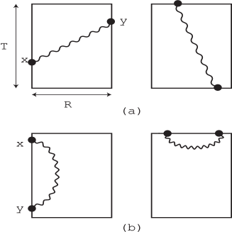
Fig. 10: A rectangular Wilson loop and the contribution to the Wilson integral in which $x$ and $y$ run over (a) opposite sides, and (b) same sides.

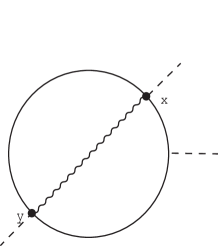
Fig. 11: A circular Wilson loop.

Next, we consider the topologically non-trivial case. We begin to estimate (9.29) for a circular Wilson loop $C$ with diameter $R$ (see Fig.11). If we avoid the coinciding case, $x=y$, $f[C]$ has a contribution only when $x$ and $y$ are at opposite ends of a diameter, i.e., $|x-y|=R$. Therefore, $D(x,y)$ and $G(x,y)$ are functions of $R$, due to translational invariance. For any $x,y\in C$, $|x-y|=R$ and

$$\oint_{C}dx^{\mu}\oint_{C}dy^{\mu}D(R)={\pi^{2}R^{2}\over 4\pi^{2}R^{2}}={1\over 4}.$$ (9.37)

Hence we obtain

$$f[C]={\lambda\over 8N}G_{C}(x,y).$$ (9.38)

It is clear that $f[C]$ is not sufficient to give a non-vanishing string tension, since $G_{C}(x,y)$ exhibits exponential decay for large $R:=|x-y|$. Note that $P_{ab}(x)$ and $\oint_{C}\omega=\int_{S}d\omega$ are U(1) gauge invariant quantities, so that $G_{C}(x,y)$ is also U(1) gauge invariant. In the large $N$ expansion, we can give a more precise estimate of the second term (see Appendix E).

Finally, we consider the topologically nontrivial case of a rectangular Wilson loop $C$ with side lengths $R$ and $T$ (see Fig.10). In this case, we cannot give a precise estimate of the second term, since we cannot perform the integration exactly. To leading order in the $1/N$ expansion, it turns out that

$$G_{C}(x,y)\cong\tilde{G}(x,y):=2(T^{A})_{ab}(T^{A})_{cd}\langle P_{ab}(x)P_{cd}(y)\rangle_{CP^{N-1}_{2}},$$ (9.39)

and that $\tilde{G}(x,y)$ decays exponentially for sufficiently large $|x-y|$ (see Appendix E). Note that $x$ and $y$ are located on the opposite sides of the rectangular Wilson loop. Therefore, there exists an uniform upper bound,

$$|\tilde{G}(x,y)|\leq\tilde{G}(R).$$ (9.40)

Hence, there exists an upper bound on $f[C]$ for a sufficiently large Wilson loop such that $T>R\gg 1$:

$$|f[C]|\leq{\lambda\over 2N}\tilde{G}(R)h[C].$$ (9.41)

Here $h[C]$ is calculated in the same way as in (9.35) by taking into account all the contributions from parallel sides $dx$ and $dy$ (see Fig.10). Therefore the second term $f[C]$ cannot give non-vanishing string tension in the topologically nontrivial case.

Thus, within this reformulation, the area law of the non-Abelian Wilson loop and the linear static potential in four-dimensional $SU(N)$ Yang-Mills theory is realized if and only if the diagonal Wilson loop ${\hbox{$\left\langle\vbox to0.0pt{}\right.\n@space$}}\exp\left(i\oint_{C}\omega\right){\hbox{$\left\rangle\vbox to0.0pt{}\right.\n@space$}}_{CP^{N-1}_{2}}$ in the two-dimensional NLS model obeys the area law

$${\hbox{$\left\langle\vbox to0.0pt{}\right.\n@space$}}\exp\left(i\oint_{C}\omega\right){\hbox{$\left\rangle\vbox to0.0pt{}\right.\n@space$}}_{CP^{N-1}_{2}}\equiv{\hbox{$\left\langle\vbox to0.0pt{}\right.\n@space$}}\exp\left(i\int_{S}\mathchar 28938\relax_{K}\right){\hbox{$\left\rangle\vbox to0.0pt{}\right.\n@space$}}_{CP^{N-1}_{2}}\sim\exp(-\sigma_{0}TR).$$ (9.42)

In other words, the area law or the linear potential between the fundamental quark and anti-quark is obtained from the topological $TQFT_{4}$ piece alone:

$$\Biggr{\langle}\exp\left(i\oint_{C}\omega\right)\Biggr{\rangle}_{TQFT_{4}}=\Biggr{\langle}\exp\left(i\oint_{C}\omega\right)\Biggr{\rangle}_{CP^{N-1}_{2}}\sim\exp(-\sigma_{0}TR).$$ (9.43)

In any case, the derivation of the area law is reduced to a two-dimensional problem.

It should be remarked that only the total static potential,

$$V(R)=\sigma_{0}R-{g^{2}(\mu)\over 4\pi}{1\over R}+{\rm const.},$$ (9.44)

is gauge invariant. Thus the linear potential piece alone is not gauge invariant. However, in the large $R$ limit, $R\rightarrow\infty$, the linear potential is dominant in $V(R)$ so that the linear potential piece becomes essentially gauge invariant.

9.2 Area law to the leading order in the large $N$ expansion

By the rescaling of the field $\phi$ in the Lagrangian (9.23), another form of the Lagrangian of the $CP^{N-1}$ model is obtained as

$${\cal L}_{CP^{N-1}}=\partial_{\mu}\bar{\phi}^{\alpha}(x)\partial_{\mu}\phi^{\alpha}(x)+{g_{0}^{2}\over 4N}(\bar{\phi}^{\alpha}(x)\partial_{\mu}\phi^{\alpha}(x)-\partial_{\mu}\bar{\phi}^{\alpha}(x)\phi^{\alpha}(x))^{2},$$ (9.45)

with the constraint

$$\phi^{\dagger}(x)\phi(x):=\bar{\phi}^{a}(x)\phi^{a}(x)={N\over g_{0}^{2}},\quad g_{0}^{2}:={g_{YM}^{2}N\over\pi}.$$ (9.46)

It is useful to consider the Schwinger parameterization, [63]

$$\phi=\pmatrix{\phi_{1}\cr\vdots\cr\phi_{N}}=e^{i\varphi}\left(1+{g_{0}^{2}\over 4N}{\bf u}^{\dagger}{\bf u}\right)^{-1}\pmatrix{{\bf u}\cr\sqrt{N\over g_{0}^{2}}(1-{g_{0}^{2}\over 4N}{\bf u}^{\dagger}{\bf u})},$$ (9.47)

where

$${\bf u}=\pmatrix{u_{1}\cr\vdots\cr u_{N-1}},\quad{\bf u}^{\dagger}{\bf u}:=\bar{u}_{\alpha}u_{\alpha}\quad(\alpha=1,\cdots,N-1).$$ (9.48)

Note that there is no constraint for the variable ${\bf u}$, since the Schwinger parameterization automatically satisfies the constraint (9.46). We can rewrite various quantities in terms of ${\bf u}$ without the constraint, e.g.,

$$\phi^{\dagger}d\phi-d\phi^{\dagger}\phi={{\bf u}^{\dagger}d{\bf u}-d{\bf u}^{\dagger}{\bf u}\over(1+{g^{2}\over 4N}{\bf u}^{\dagger}{\bf u})^{2}}+2i{N\over g_{0}^{2}}d\varphi.$$ (9.49)

Then the $U(1)$ gauge field $V=V_{\mu}dx^{\mu}$ in the $CP^{N-1}$ model is written as

$$V:={i\over 2}{g_{0}^{2}\over N}(\phi^{\dagger}d\phi-d\phi^{\dagger}\phi)={i\over 2}{g_{0}^{2}\over N}{{\bf u}^{\dagger}d{\bf u}-d{\bf u}^{\dagger}{\bf u}\over(1+{g_{0}^{2}\over 4N}{\bf u}^{\dagger}{\bf u})^{2}}-d\varphi.$$ (9.50)

We identify the complex coordinate $w$ in the Kähler manifold with the Schwinger variable as

$$w_{\alpha}=\sqrt{g_{0}^{2}\over N}{u_{\alpha}\over 1-{g_{0}^{2}\over 4N}{\bf u}^{\dagger}{\bf u}}.\quad(\alpha=1,\cdots,N-1)$$ (9.51)

This leads to

$$\bar{w}_{\alpha}dw_{\alpha}-d\bar{w}_{\alpha}w_{\alpha}={1\over(1-{g_{0}^{2}\over 4N}{\bf u}^{\dagger}{\bf u})^{2}}{g_{0}^{2}\over N}(\bar{u}_{\alpha}du_{\alpha}-d\bar{u}_{\alpha}u_{\alpha}),$$ (9.52)

and

$$1+\bar{w}_{\alpha}w_{\alpha}={(1+{g_{0}^{2}\over 4N}{\bf u}^{\dagger}{\bf u})^{2}\over(1-{g_{0}^{2}\over 4N}{\bf u}^{\dagger}{\bf u})^{2}}.$$ (9.53)

Then we find the following expression for $\omega$ in terms of $u$:

$$\omega:={i\over 2}{\bar{w}_{\alpha}dw_{\alpha}-d\bar{w}_{\alpha}w_{\alpha}\over 1+\bar{w}_{\alpha}w_{\alpha}}={i\over 2}{g_{0}^{2}\over N}{{\bf u}^{\dagger}d{\bf u}-d{\bf u}^{\dagger}{\bf u}\over(1+{g_{0}^{2}\over 4N}{\bf u}^{\dagger}{\bf u})^{2}}.$$ (9.54)

Thus the connection one-form is given by

$$V={i\over 2}{\bar{w}_{\alpha}dw_{\alpha}-d\bar{w}_{\alpha}w_{\alpha}\over 1+\bar{w}_{\alpha}w_{\alpha}}-d\varphi=\omega-d\varphi,$$ (9.55)

and the Abelian curvature two-form is equal to the Kähler two-form:

$$dV=d\omega=\mathchar 28938\relax_{K}=ig_{\alpha\bar{\beta}}dw_{\alpha}\wedge d\bar{w}_{\beta},$$ (9.56)

$$g_{\alpha\bar{\beta}}={\mathchar 28929\relax\delta_{\alpha\beta}-\bar{w}_{\alpha}w_{\beta}\over\mathchar 28929\relax},\quad\mathchar 28929\relax:=1+|||w|||^{2}.$$ (9.57)

By way of the variable $u$, we have found that the connection one-form $\omega$ appearing in the NAST is equal to the gauge-invariant part of $V$. Therefore the diagonal Wilson loop for $CP^{N-1}$ model is equal to

$${\hbox{$\left\langle\vbox to0.0pt{}\right.\n@space$}}\exp\left(i\oint_{C}\omega\right){\hbox{$\left\rangle\vbox to0.0pt{}\right.\n@space$}}_{CP^{N-1}}={\hbox{$\left\langle\vbox to0.0pt{}\right.\n@space$}}\exp\left(i\oint_{C}V\right){\hbox{$\left\rangle\vbox to0.0pt{}\right.\n@space$}}_{CP^{N-1}}.$$ (9.58)

For the $CP^{1}$ model, this reduces to $V$ (6.51) in Ref.? for $G=SU(2)$.

The expectation value $\langle\exp\left(i\oint_{C}V\right)\rangle_{CP^{N-1}}$ is calculated in Appendix D in the large $N$ expansion in a manner based on pioneering works. [56, 57, 58] The result agrees with the result of Campostrini and Rossi.[60] To leading order in the $1/N$ expansion, the Wilson loop obeys the area law for all non-self-intersecting loops:

$${\hbox{$\left\langle\vbox to0.0pt{}\right.\n@space$}}\exp\left(i\oint_{C}V\right){\hbox{$\left\rangle\vbox to0.0pt{}\right.\n@space$}}_{CP^{N-1}}=\exp\left[-{6\pi\over N}m_{\phi}^{2}|{\rm Area}(C)|\right],$$ (9.59)

where

$$m_{\phi}^{2}=\mu^{2}\exp\left[-{2\pi^{2}\over g^{2}(\mu)}\right].$$ (9.60)

Thus the string tension is obtained as

$$\sigma_{0}={6\pi\over N}m_{\phi}^{2}.$$ (9.61)

Here $m_{\phi}$ is the mass of the $CP^{N-1}$ field $\phi$. The $m_{\phi}^{2}$ is equal to the vacuum expectation value $\langle\sigma(x)\rangle$ of the Lagrange multiplier field $\sigma$ from the correspondence $\sigma(x)\bar{\phi}(x)\phi(x)\rightarrow m_{\phi}^{2}\bar{\phi}(x)\phi(x)$. In the propagator of the vector field $V$, a massless pole appears. Hence, the auxiliary vector field $V$ becomes a dynamical gauge field, giving rise to a linear confining potential between $\phi$ and $\bar{\phi}$. On the other hand, the Lagrange multiplier field $\sigma$ for the constraint (9.46) becomes massive, so that it does not contribute to the confining potential between $\phi$ and $\bar{\phi}$. Thus we have completed a proof of quark confinement in four-dimensional $SU(N)$ Yang-Mills theory based on the Wilson criterion to leading order in the large $N$ expansion within our reformulation of the Yang-Mills theory.

10 Remarks

Some remarks are in order to avoid confusion.

10.1 Calculating gauge invariant quantity in the gauge non-invariant theory

The Wilson loop operator $W_{C}[{\cal A}]$ is invariant under the gauge transformation denoted by $U(x)$, which is defined by the decomposition of the variable in (7.1) or (7.10), since it is a gauge-invariant quantity. Therefore, the expression of the Wilson loop operator given by the non-Abelian Stokes theorem derived in this paper is also invariant under arbitrary (i.e., infinitesimal and finite) gauge transformation. Therefore, the variable $U(x)$ does not contribute to the Wilson loop operator, and we can write

$$W_{C}[{\cal A}]=W_{C}[{\cal V}],$$ (10.1)

which is a mathematical identity. This is indeed the situation before taking the expectation value $\langle W_{C}[{\cal A}]\rangle_{YM}$ in terms of the Yang-Mills theory. However, this seems to contradict the claim of this paper; the area law can be derived from the contribution of the topologically non-trivial degrees of freedom expressed by the variable $U(x)$, which is described by the TQFT. In fact, we have used the formula (7.19) to calculate the expectation value of the Wilson loop operator in $\S$ 8. Therefore, if we set

$$g({\cal V},U)=g({\cal V})=W_{C}[{\cal V}],\quad h(U)=1,$$ (10.2)

in the expectation value $\langle\cdot\rangle_{YM}$, we would obtain the inconsistent result

$$\langle W_{C}[{\cal A}]\rangle_{YM}=\langle W_{C}[{\cal V}]\rangle_{pYM}\langle 1\rangle_{TQFT}=\langle W_{C}[{\cal V}]\rangle_{pYM}?$$ (10.3)

since this implies that there is no contribution from the topological part expressed by $U$ and that the Wilson loop can be calculated by the perturbative part only.

This apparent contradiction can be understood as follows. Elimination of the $U$-dependence is possible only when the gauge theory itself is formulated in a gauge invariant way, just as the lattice gauge theory can be written in a manifestly gauge invariant manner without gauge fixing. In such a case, we can perform the gauge transformation so that a gauge invariant quantity, e.g., the Wilson loop, has no dependence on $U(x)$ also in the expectation value. However, our strategy is totally different from this case. That is to say, we calculate the gauge-invariant quantity using the gauge fixed (i.e, gauge non-invariant) theory, where the off-diagonal components and the diagonal components are subject to different gauge fixing conditions. Therefore, the total action $S_{YM}^{tot}[{\cal A},\cdots]=S_{YM}[{\cal A}]+S_{GF+FP}[{\cal A},\cdots]$ obtained by adding the GF+FP term $S_{GF+FP}[{\cal A},\cdots]$ to the Yang-Mills action $S_{YM}[{\cal A}]$ does not have the same form as the gauge-transformed total action $S_{YM}^{tot}[{\cal V},B,C,\bar{C}]$ obtained by the gauge rotation $U$, although $S_{YM}[{\cal A}]=S_{YM}[{\cal V}]$. In this sense,

$$\langle W_{C}[{\cal A}]\rangle_{YM}\not=\langle W_{C}[{\cal V}]\rangle_{YM},$$ (10.4)

where

$$\langle W_{C}[{\cal A}]\rangle_{YM}:=Z_{YM}^{-1}\int{\cal D}{\cal A}_{\mu}\cdots\exp\{iS_{YM}^{tot}[{\cal A},\cdots]\}W_{C}[{\cal A}].$$ (10.5)

Thus it should be remarked that the formula (7.19) holds only when the field variable ${\cal A}$ is separated into ${\cal V}$ and $U$ and at the same time the respective component is identified with the topologically trivial (perturbative) and non-trivial (non-perturbative) components, respectively, where the ${\cal V}$-dependent part is calculated using perturbative Yang-Mills (pYM) theory. This is an assumption of our approach. In this sense, Eq. (7.19) holds under this assumption and it is not a mathematical identity. In our approach, an arbitrary gauge transformation is not allowed under the functional of the expectation value, i.e., $\langle\cdot\rangle_{YM}$, once the respective component is identified with the relevant degrees of freedom in Yang-Mills theory. (Thus, if we wish to change the integration variable as in (10.2), the total Yang-Mills theory should be modifed simultaneously. This leads to a more complicated theory.) In this paper we have fixed the gauge degrees of freedom for the variable $U(x)$ using the modified MA gauge. In other words, we have chosen a specific field configuration of $\{U(x)\}$ to calculate the physical quantity in such a way that the $U$-dependence is controlled by the MA gauge fixing term. This is an essential point of our strategy. In this sense, the physics enters in when we consider the expectation value.

10.2 The Gribov problem and dimensional reduction

Dimensional reduction of the Parisi-Sourlas type was applied to the random field Ising model [73] and scalar field theories with random external sources [74, 75, 76] based on non-perturbative [74, 75] and rigorous methods.[73, 76] In these models it has been recognized [77, 78] that the Parisi-Sourlas correspondence (between random systems in $d$ dimensions and the corresponding pure systems in $d-2$ dimensions, or supersymmetric theory in $d$ dimensions and the corresponding bosonic theory in $d-2$ dimensions) is exact only in the case of unique solutions to the classical equation of motion. In fact, it was rigorously shown [73] that the three-dimensional Ising model in a random magnetic field exhibits long-range order at zero temperature and small disorder. This implies that the lower critical dimension $d_{\ell}$ for this model is 2 (ruling out $d_{\ell}=3$), where the lower-critical dimension is the dimension above which ($d>d_{\ell}$) long-range ferromagnetic order can exist. Therefore, this result contradicts the naive prediction [72] between the random field Ising model in $d$ dimensions and the pure Ising model in $d-2$ dimensions.

In gauge theories, a similar problem can in principle arise due to the existence of Gribov copies, although much is not known on this issue. Indeed, it is known [80] that Gribov copies exist for the naive MA gauge. On the other hand, it is not known whether the modified MA gauge with $OSp(D|2)$ symmetry possesses the Gribov copies or not. If Gribov copies exist, first of all, the naive BRST formulation breaks down. Even if a modified BRST formulation can exist, the BRST symmetry can be spontaneously broken,[79] at least in the topological sector (described by the modified MA gauge action), where the large (or finite) gauge transformation with non-trivial winding number plays a crucial role. In this case, the vacuum in the topological sector is not annihilated by the BRST charge $Q_{B}$ (i.e., $Q_{B}|0\rangle_{TQFT}\not=0$), whereas the perturbative sector (in which there exist small quantum fluctuation around an arbitrary but fixed topological background) is characterized by the unbroken BRST charge, i.e., $Q_{B}|0\rangle_{pYM}=0$. Even in this case, dimensional reduction should take place, since we have used neither the field equations nor the above property of the BRST charge acting on the state. In other words, the dimensional reduction is an origin of the spontaneous breaking of the BRST symmetry (see Refs.?, ?). Moreover, the BRST symmetry can also be broken by other mechanisms, e.g., radiative corrections.

In any case, the spontaneous breaking of the BRST symmetry in the topological sector implies that the expectation value of the gauge invariant operator depends on the gauge fixing parameter $\alpha$ for the topological sector. In this case, we can not conclude the $\alpha$-independence of the physical (gauge-invariant) quantities. Rather, the value of $\alpha$ should be determined as a physical parameter by the theory [43] or experiments. This is reasonable if we believe that the real world is described by a unique quantum theory and that nature is realized at an appropriate gauge fixing, since the classical theory does not really exist in nature, and hence ambiguities arising in the quantization are absent from the beginning. It is a challenge to give a definite answer to these questions. The author would like to thank the referee for pointing out the Gribov problem as an obstacle to the dimensional reduction.

11 Conclusion and discussion

We have given a new version of the non-Abelian Stokes theorem for $G=SU(N)$ with $N\geq 2$ which reduces to the previous result [15] for $SU(2)$. This version of the non-Abelian Wilson loop is very helpful to see the role played by the magnetic monopole in the calculation of the expectation value of the non-Abelian Wilson loop. Combining this non-Abelian Stokes theorem with the Abelian-projected effective gauge theory for $SU(N)$, we have explained the Abelian dominance for the Wilson loop in $SU(N)$ Yang-Mills gauge theory. For $SU(N)$ with $N\geq 3$, we must distinguish the maximal stability group $\tilde{H}$ and the residual gauge group $H$, which is taken to be the maximal torus group $H=U(1)^{N-1}$.

In order to demonstrate the magnetic monopole dominance and the area law of the Wilson loop, we have used a novel reformulation of the Yang-Mills theory which has been proposed by one of the authors.[13] This reformulation is based on the identification of the Yang-Mills theory with the perturbative deformation of a topological quantum field theory. This framework deals with the gauge action $S_{YM}$ and the gauge-fixing action $S_{GF}$ on an equal footing. The gauge action is characterized from the viewpoint of the geometry of connections. On the other hand, the gauge-fixing part is related to the topological invariant (Euler characteristic) determined by a global topology. Therefore, the gauge-fixing part can have a geometric meaning from a global viewpoint. This point has not been emphasized in textbooks on quantum field theory. (See Ref.? for more details.)

Our approach relies heavily on a specific gauge, the MA gauge. In spite of the absence of an elementary scalar field in Yang-Mills theory, the MA gauge allows the existence of the magnetic monopole. The magnetic monopole is considered as a topological soliton composed of gauge degrees of freedom, providing the composite scalar field. At least in this gauge, (Parisi-Sourlas) dimensional reduction occurs due to the supersymmetry hidden in the gauge fixing part in the MA gauge. By making use of the non-Abelian Stokes theorem within this reformulation of the Yang-Mills theory, the derivation of the area law of the non-Abelian Wilson loop in four-dimensional Yang-Mills theory has been reduced to the two-dimensional problem of calculating the expectation value of the Abelian Wilson loop in the coset $G/H$ non-linear sigma model. This is the main result of this article.

In particular, in order to demonstrate confinement of the fundamental quark in the four-dimensional $SU(N)$ Yang-Mills theory in the MA gauge, we have only to consider the two-dimensional $CP^{N-1}$ model. From the topological point of view, the Abelian Wilson loop is equivalent to the area integral (enclosed by the Wilson loop) of the instanton density in the two-dimensional NLS model. This implies that the calculation of the magnetic monopole contribution to the Wilson loop in four-dimensional Yang-Mills theory was translated into that of the instanton contribution in the two-dimensional NLS model when the Wilson loop is contained in the two-dimensional plane, i.e. when the Wilson loop is planar. In addition, the two-dimensional instanton is considered as a subclass of the four-dimensional Yang-Mills instanton (see Ref.?). This suggests that the area law of the Wilson loop can be derived by taking into account the contributions of a restricted class of Yang-Mills instantons. A Monte Carlo simulation on a lattice will be efficient in confirming this dimensionally reduced picture of quark confinement.[64]

Moreover, naive instanton calculus (the dilute gas approximation) in the coset NLS model leads to the area law of the Wilson loop of the original four-dimensional Yang-Mills theory. Improvements of the dilute gas approximation are necessary to confirm the area law based on the above picture. However, this is rather difficult, as found more than twenty years ago.[55] An advantage of the extension of the above strategy to $SU(N)$ with arbitrary $N$ is that the large $N$ systematic expansion can be used in the calculation of the Wilson loop, and that the area law of the Wilson loop has been demonstrated. These results confirm the area law of the Wilson loop. It is known that the large $N$ Yang-Mills theory is related to the string theory. The correspondence between instanton calculus and the large $N$ expansion and a related issue in the large $N$ expansion in Yang-Mills theory will also be discussed in a subsequent article.[43] These considerations should shed more light on the confining string picture.[65]

A Normalization of the Coherent State

In this appendix we derive the normalization facter $N$ of coherent state $\left|\xi,\mathchar 28931\relax\right>$ which parametrizes $G/\tilde{H}$,

$$N :=\left<\mathchar 28931\relax\right|\exp{[\bar{\tau}_{\alpha}E_{\alpha}]}\exp{[\tau_{\beta}E_{-\beta}]}\left|\mathchar 28931\relax\right>$$ (A.1)

$$= \sum_{K,L=0}^{\infty}\frac{1}{K!}\frac{1}{L!}\bar{\tau}_{\alpha^{1}}\ldots\bar{\tau}_{\alpha^{K}}\tau_{\beta^{1}}\ldots\tau_{\beta^{L}}\left<\mathchar 28931\relax\right|E_{\alpha^{1}}\ldots E_{\alpha^{K}}E_{-\beta^{1}}\ldots E_{-\beta^{L}}\left|\mathchar 28931\relax\right>.$$ (A.2)

A.1 $SU(3)$ coherent state

We use the positive root $\alpha^{(i)}$ and Dynkin index $[m,n]$ in $SU(3)$, which are defined by Fig.3 and (3.13). This definition may be rewritten as

$$\alpha^{(1)}\cdot\vec{\mathchar 28931\relax}=\frac{m}{2},\quad\ \alpha^{(3)}\cdot\vec{\mathchar 28931\relax}=\frac{n}{2}.$$ (A.3)

For $[m,n]=[m,0]$ (resp., $[0,n]$), $\alpha$ and $\beta$ run over $1,2$ (resp., $2,3$). Then the corresponding coherent state parametrizes $CP^{2}$. From the orthogonality of the states which span the representation space, the terms contributing to $N$ in (A.1) must satisfy the condition

$$\alpha^{1}+\ldots+\alpha^{K}-\beta^{1}-\ldots-\beta^{L}=0.$$ (A.4)

In the $[m,0]$ case, this condition implies that the number of $\alpha^{(1)}$ and $\alpha^{(2)}$ in $K$ positive roots is equal to that of $\alpha^{(1)}$ and $\alpha^{(2)}$ in $L$ negative roots. Since $[E_{1},E_{2}]=0$, we have only to estimate the terms

$$N_{k,l}:=\left<\mathchar 28931\relax\right|\underbrace{E_{1}\ldots E_{1}}_{k}\underbrace{E_{2}\ldots E_{2}}_{l}\underbrace{E_{-2}\ldots E_{-2}}_{l}\underbrace{E_{-1}\ldots E_{-1}}_{k}\left|\mathchar 28931\relax\right>.$$ (A.5)

We begin with the term

$$N_{0,l} = \left<\mathchar 28931\relax\right|\underbrace{E_{2}\ldots E_{2}}_{l}\underbrace{E_{-2}\ldots E_{-2}}_{l}\left|\mathchar 28931\relax\right>=N_{0,l}\left<\mathchar 28931\relax-l\alpha^{(2)}|\mathchar 28931\relax-l\alpha^{(2)}\right>,$$ (A.6)

where we have used in the last equality the fact that $E_{-2}\ldots E_{-2}\left|\mathchar 28931\relax\right>$ has a weight $\mathchar 28931\relax-l\alpha^{(2)}$ and is proportional to the state $\left|\mathchar 28931\relax-l\alpha^{(2)}\right>$, which is normalized as

$$\left<\mathchar 28931\relax-l\alpha^{(2)}{\hbox{$\left|\vbox to0.0pt{}\right.\n@space$}}\mathchar 28931\relax-l\alpha^{(2)}\right>=1.$$ (A.7)

Exchanging the rightmost $E_{2}$ with $E_{-2}$ and using

$$[E_{2},E_{-2}] = \alpha^{(2)}\cdot H,$$ (A.8)

$$\alpha^{(2)}\cdot H\left|\mathchar 28931\relax-j\alpha^{(2)}\right> = (\frac{m}{2}-j)\left|\mathchar 28931\relax-j\alpha^{(2)}\right>,\quad(0<j<m)$$ (A.9)

we obtain the recursion relation for $N_{0,l}$,

$$N_{0,l} = \left\{\frac{m}{2}-(l-1)\right\}N_{0,l-1}+\left<\mathchar 28931\relax\right|\underbrace{E_{2}\ldots E_{2}}_{l-1}E_{-2}E_{2}\underbrace{E_{-2}\ldots E_{-2}}_{l-1}\left|\mathchar 28931\relax\right>$$ (A.10)

$$= \left(\frac{m}{2}-(l-1)+\frac{m}{2}-(l-2)+\cdots+\frac{m}{2}\right)N_{0,l-1}$$

$$= \frac{l(m-l+1)}{2}N_{0,l-1},$$

where we have used $E_{2}\left|\mathchar 28931\relax\right>=0$. From this relation and from $N_{0,0}=\left<\mathchar 28931\relax|\mathchar 28931\relax\right>=1$, we obtain

$$N_{0,l}=\frac{(l!)^{2}{m\choose l}}{2^{l}}.$$ (A.11)

Similarly,

$$N_{k,0}=\frac{(k!)^{2}{m\choose k}}{2^{k}}.$$ (A.12)

For the general terms (A.5), we have

$$N_{k,l} = N_{k,0}\left<\mathchar 28931\relax-k\alpha^{(1)}\right|\underbrace{E_{2}\ldots E_{2}}_{l}\underbrace{E_{-2}\ldots E_{-2}}_{l}\left|\mathchar 28931\relax-k\alpha^{(1)}\right>$$ (A.13)

$$= N_{k,0}\frac{k(m-k-l+1)}{2}\left<\mathchar 28931\relax-k\alpha^{(1)}\right|\underbrace{E_{2}\ldots E_{2}}_{l-1}\underbrace{E_{-2}\ldots E_{-2}}_{l-1}\left|\mathchar 28931\relax-k\alpha^{(1)}\right>$$

$$= \frac{(k!)^{2}{m\choose k}}{2^{k}}\frac{(l!)^{2}{m-k\choose l}}{2^{l}}.$$

Finally, the normalization factor $N$ is given by

$$N = \sum_{k=0}^{\infty}\sum_{l=0}^{\infty}\frac{1}{(k+l)!^{2}}{k+l\choose l}\underbrace{\bar{\tau}_{2}\ldots\bar{\tau}_{2}}_{l}\underbrace{\bar{\tau}_{1}\ldots\bar{\tau}_{1}}_{k}\underbrace{\tau_{2}\ldots\tau_{2}}_{l}\underbrace{\tau_{1}\ldots\tau_{1}}_{k}N_{k,l}$$ (A.14)

$$= \sum_{k=0}^{n}\sum_{l=0}^{n-k}(\frac{\bar{\tau}_{2}\tau_{2}}{2})^{l}(\frac{\bar{\tau}_{1}\tau_{1}}{2})^{k}{m\choose k}{m-k\choose l}$$

$$= \left(1+(\frac{\bar{\tau}_{1}\tau_{1}}{2})+(\frac{\bar{\tau}_{2}\tau_{2}}{2})\right)^{m}$$

$$= \left(1+(\bar{w}_{1}w_{1})+(\bar{w}_{2}w_{2})\right)^{m}=\exp{K_{CP^{2}}(\bar{w},w)},$$

where $w_{1}:=\tau_{1}/\sqrt{2}\ w_{2}:=\tau_{2}/\sqrt{2}$, and $K_{CP^{2}}(w)$ is the Kähler potential of $CP^{2}$.

For $F_{2}$, i.e., $mn\neq 0$, $\alpha$ and $\beta$ in (A.1) run over $1,2,3$. Here we apply almost the same steps as in the case of $CP^{2}$. The result is

$$N := \left<\mathchar 28931\relax\right|\exp{\sum_{\alpha=1}^{3}[\bar{\tau}_{\alpha}E_{\alpha}]}\exp{\sum_{\beta=1}^{3}[\tau_{\beta}E_{-\beta}]}\left|\mathchar 28931\relax\right>$$ (A.15)

$$= \left(1+|\frac{\tau_{1}}{\sqrt{2}}|^{2}+|\frac{\tau_{2}}{\sqrt{2}}+\frac{\tau_{1}\tau_{3}}{4}|^{2}\right)^{m}\left(1+|\frac{\tau_{3}}{\sqrt{2}}|^{2}+|\frac{\tau_{2}}{\sqrt{2}}-\frac{\tau_{1}\tau_{3}}{4}|^{2}\right)^{n}$$

$$= \left(1+|w_{1}|^{2}+|w_{2}|^{2})\right)^{m}\left(1+|w_{3}|^{2}+|w_{2}-w_{1}w_{3}|^{2}\right)^{n}$$

$$= \exp{K_{F_{2}}(\bar{w},w)},$$

where $w_{1}:=\tau_{1}/\sqrt{2},\ w_{2}:=\tau_{2}/\sqrt{2}+\tau_{1}\tau_{3}/4,\ w_{3}:=\tau_{3}/\sqrt{2}$.

A.2 $SU(N)$ coherent state

In $SU(N)$, the simple root $\alpha^{i}$ and the Dynkin index $[m_{1},\cdots m_{N-1}]$ are defined by (3.47) and $\alpha^{i}\cdot\mathchar 28931\relax:=m_{i}/2$. In general, the roots $E_{\pm\alpha}$ belonging to the coset group $G/\tilde{H}$ are not orthogonal to the highest weight $\mathchar 28931\relax.$ We restrict our consideration to only the case of $[m,0,\cdots,0]$, in which case only $\alpha^{1}$ is not orthogonal to $\mathchar 28931\relax$. Any positive root $\tilde{\alpha}$ is given by a linear combination of simple roots $\alpha^{i}$. The positive roots $\tilde{\alpha}_{i}$ in (A.1) are not orthogonal to $\mathchar 28931\relax$, so they must include $\alpha^{1}$. It turns out that such roots are given by $\tilde{\alpha}_{i}:=\alpha^{1}+\cdots+\alpha^{i}\ (i=1,\cdots N-1)$ , which are realized by $\left(E_{\tilde{\alpha}_{i}}\right)_{kl}=\delta_{1,k}\delta_{i+1,l}/\sqrt{2}$ in the ${\bf N}$ representation. The corresponding coherent state parametrizes $CP^{N-1}$. We can easily extend the $CP^{2}$ case to that of $CP^{N-1}$ using the fact that $[E_{\tilde{\alpha}_{i}},E_{\tilde{\alpha}_{j}}]=0$ and $\tilde{\alpha}_{i}\cdot\vec{\mathchar 28931\relax}=m/2$. (This situation is same as in the $SU(3)$ case, i.e., $[E_{1},E_{2}]=0$, and $\alpha^{(1)}\cdot\vec{\mathchar 28931\relax}=\alpha^{(2)}\cdot\vec{\mathchar 28931\relax}=m/2$.) Thus we obtain

$$N := \left<\mathchar 28931\relax\right|\exp{\sum_{i=1}^{N-1}[\bar{\tau}_{i}E_{\tilde{\alpha}_{i}}]}\exp{\sum_{j=1}^{N-1}[\tau_{j}E_{-\tilde{\alpha}_{j}}]}\left|\mathchar 28931\relax\right>$$ (A.16)

$$= \left(1+\sum_{i=1}^{N-1}(\frac{\bar{\tau}_{i}\tau_{i}}{2})\right)^{m}=:\left(1+\sum_{i=1}^{N-1}(\bar{w}_{i}w_{i})\right)^{m}$$

$$= \exp{K_{CP^{N-1}}(\bar{w},w)}.$$

B From $CP^{1}$ to $CP^{2}$

For an arbitrary element $(\phi_{1},\phi_{2},\phi_{3})$ of $W$,

$$W={\bf C}^{3}-(0,0,0),$$ (B.1)

the entire set of ratios $\phi_{1}:\phi_{2}:\phi_{3}$ is called the complex projective plane and is denoted by $P^{2}({\bf C})$ or ${\bf C}P^{2}$:

$$(\alpha\phi_{1}:\alpha\phi_{2}:\alpha\phi_{3})=(\phi_{1}:\phi_{2}:\phi_{3}),\quad\alpha\in{\bf C},\quad\alpha\not=0.$$ (B.2)

Defining the subset $U_{a}(a=1,2,3)$ of ${\bf C}P^{2}$ as

$$U_{a}=\{(\phi_{1}:\phi_{2}:\phi_{3})\in{\bf C}P^{2};\phi_{a}\not=0\}\subset{\bf C}P^{2},$$ (B.3)

we observe that

$$(\phi_{1}:\phi_{2}:\phi_{3})=\left(1:{\phi_{2}\over\phi_{1}}:{\phi_{3}\over\phi_{1}}\right)\in U_{1}.$$ (B.4)

The mapping $\varphi_{1}$ from $U_{1}$ to ${\bf C}^{2}$,

$$\varphi_{1}:(\phi_{1}:\phi_{2}:\phi_{3})\in U_{1}\rightarrow\left({\phi_{2}\over\phi_{1}}:{\phi_{3}\over\phi_{1}}\right)\in{\bf C}^{2},$$ (B.5)

is a bijection, i.e., a surjection (onto-mapping) and injection (one-to-one mapping). The inverse mapping is given by

$$\varphi_{1}^{-1}:(x,y)\in{\bf C}^{2}\rightarrow(1:x:y)\in U_{1}.$$ (B.6)

Similarly, the following maps $\varphi_{2}$ and $\varphi_{3}$ are also bijections from $U_{2}$ and $U_{3}$ to ${\bf C}^{2}$:

$$\varphi_{2}:(\phi_{1}:\phi_{2}:\phi_{3})\in U_{2}\rightarrow\left({\phi_{1}\over\phi_{2}}:{\phi_{3}\over\phi_{2}}\right)\in{\bf C}^{2},$$ (B.7)

$$\varphi_{3}:(\phi_{1}:\phi_{2}:\phi_{3})\in U_{3}\rightarrow\left({\phi_{1}\over\phi_{3}}:{\phi_{2}\over\phi_{3}}\right)\in{\bf C}^{2}.$$ (B.8)

Since

$${\bf C}P^{2}=U_{1}\cup\{(0:\phi_{2}:\phi_{3})\},\quad(\phi_{2}:\phi_{3})\not=0,$$ (B.9)

$(\phi_{2}:\phi_{3})$ determines a point in ${\bf C}P^{2}$. Conversely, for a point $(b_{1}:b_{2})$ in ${\bf C}P^{1}$, $(0:b_{1}:b_{2})$ defines a point in ${\bf C}P^{2}-U_{1}$. Thus the map

$$(0:\phi_{2}:\phi_{3})\in{\bf C}P^{2}-U_{1}\rightarrow(\phi_{2}:\phi_{3})\in{\bf C}P^{1}$$ (B.10)

is one-to-one and onto. Then we can identify ${\bf C}P^{2}-U_{1}$ with ${\bf C}P^{1}$ as ${\bf C}P^{2}-U_{1}\cong{\bf C}P^{1}$.

On the other hand, the identification of $U_{1}$ and ${\bf C}^{2}$, $U_{1}\cong{\bf C}^{2}$, by the mapping $\varphi_{1}$ leads to

$${\bf C}P^{2}=U_{1}\cup{\bf C}P^{1}\cong{\bf C}^{2}\cup{\bf C}P^{1}.$$ (B.11)

Using ${\bf C}P^{1}={\bf C}^{1}\cup\{(0:1)\}$, we can write ${\bf C}P^{2}={\bf C}^{2}\cup{\bf C}^{1}\cup\{(0:1)\}\equiv{\bf C}^{2}\cup{\bf C}^{1}\cup{\bf C}^{0}.$ ${\bf C}P^{2}-U_{1}$ is called the “line at infinity” and is denoted by $\ell_{\infty}$, ${\bf C}P^{2}-U_{1}=\ell_{\infty}$. Thus we can also write

$${\bf C}P^{2}=U_{1}\cup\ell_{\infty},\quad U_{1}\cong C^{2},\quad\ell_{\infty}\cong{\bf C}P^{1},$$ (B.12)

where ${\bf C}^{2}$ is called the “complex affine plane”. The homogeneous coordinates $(\phi_{1}:\phi_{2}:\phi_{3})$ are related to an element $(x,y)$ in the affine plane as

$$x={\phi_{2}\over\phi_{1}},\quad y={\phi_{3}\over\phi_{1}},\quad\ell_{\infty}\cong\{\phi_{1}=0\}.$$ (B.13)

${\bf C}P^{2}$ is obtained as ${\bf C}P^{2}={\cal U}\cup{\cal V}\cup{\cal W}$ by gluing the three affine planes ${\cal U},{\cal V}$ and ${\cal W}$ using the relations

$$u_{1}={1\over v_{1}},\quad u_{2}={v_{2}\over v_{1}},\quad v_{1}={w_{1}\over w_{2}},\quad v_{2}={1\over w_{2}},\quad w_{1}={1\over u_{2}},\quad w_{2}={u_{1}\over u_{2}},$$ (B.14)

where $(u_{1},u_{2}),(v_{1},v_{2})$ and $(w_{1},w_{2})$ are the coordinates of ${\cal U},{\cal V}$ and ${\cal W}$ defined in terms of homogeneous coordinates of ${\bf C}P^{2}$ as

$$(u_{1},u_{2})=\left({\phi_{2}\over\phi_{1}},{\phi_{3}\over\phi_{1}}\right),\quad(v_{1},v_{2})=\left({\phi_{1}\over\phi_{2}},{\phi_{3}\over\phi_{2}}\right),\quad(w_{1},w_{2})=\left({\phi_{1}\over\phi_{3}},{\phi_{2}\over\phi_{3}}\right).$$ (B.15)

Note that the method of gluing affine planes is not unique. In fact, ${\bf C}P^{2}$ can be obtained from the following gluing:

$$u_{1}={w_{2}\over w_{1}},\quad u_{2}={1\over w_{1}},\quad v_{1}={1\over u_{1}},\quad v_{2}={u_{2}\over u_{1}},\quad w_{1}={v_{1}\over v_{2}},\quad w_{2}={1\over v_{2}}.$$ (B.16)

C Nonlinear Sigma Model of the Flag Space

C.1 Correspondence between $SU(N)/T$ and $SL(N,C)/B$

When an element $\xi$ in $F_{N-1}$ is expressed by the complex coordinate,

$$\xi=\pmatrix{1&w_{1}&w_{2}&\cdots&\cdots&w_{n}\cr 0&1&w_{n+1}&\cdots&\cdots&w_{2n-1}\cr 0&0&1&w_{2n}&\cdots&w_{3n-3}\cr&&&&&\cr\vdots&\vdots&\vdots&\vdots&\vdots&\vdots\cr&&&&&\cr 0&0&\cdots&0&1&w_{n(n+1)/2}\cr 0&0&\cdots&\cdots&0&1\cr}^{T}\in F_{n},$$ (C.1)

we find $\det\xi=1$. Hence $\xi$ is an element of $SL(N,C)$. There is the isomorphism $SU(N)/T\cong SL(N,C)/B$. However, $\xi$ in this form is not necessarily unitary. The corresponding unitary matrix $V\in SU(N)$ is obtained as follows. First, $\xi$ as an element of $SL(N,C)$ is expressed in terms of the column vectors:

$$\xi=(E_{1},E_{2},\cdots,E_{N})\in SL(N,C)=SU(N)^{C}.$$ (C.2)

By applying the Gramm-Schmidt orthogonalization, we can obtain a set of mutually orthogonal vectors $(E_{1}^{\prime},E_{2}^{\prime},\cdots,E_{N}^{\prime})$ from $(E_{1},E_{2},\cdots,E_{N})$ as

$$E_{1}^{\prime} := E_{1},$$

$$E_{2}^{\prime} := E_{2}-{(E_{2},E_{1}^{\prime})\over(E_{1}^{\prime},E_{1}^{\prime})}E_{1}^{\prime},$$

$$\vdots$$

$$E_{N}^{\prime} := E_{N}-{(E_{N},E_{N-1}^{\prime})\over(E_{N-1}^{\prime},E_{N-1}^{\prime})}E_{N-1}^{\prime}-\cdots-{(E_{N},E_{1}^{\prime})\over(E_{1}^{\prime},E_{1}^{\prime})}E_{1}^{\prime},$$ (C.3)

where the inner product is defined by $(E_{i},E_{j}):=E_{i}^{T}\cdot\bar{E}_{j}.$ Using the normalized vectors $e_{j}:=E_{j}^{\prime}/||E_{j}^{\prime}||$, we obtain an element in $SU(N)$,

$$V=(e_{1},e_{2},\cdots,e_{N})\in SU(N).$$ (C.4)

In fact, $\det V=1$ and $V$ is unitary, since

$$V^{\dagger}V=\pmatrix{\bar{e}_{1}^{T}\cr\vdots\cr\bar{e}_{N}^{T}}(e_{1},e_{2},\cdots,e_{N}),\quad(V^{\dagger}V)_{ij}=\bar{e}_{i}^{T}\cdot e_{j}=(e_{i},e_{j})=\delta_{ij}.$$ (C.5)

In general, the unitary matrix $V$ is related to its complexfication $V^{C}$ by

$$V=V^{C}B,\quad V\in SU(N),\quad V^{C}\in SL(N,C),$$ (C.6)

where $B$ is an upper triangular matrix. This is nothing but the Iwasawa decomposition. Since the upper triangular matrices form a group, we have

$$V^{C}=VB^{-1}=VB^{\prime},$$ (C.8)

where $B^{\prime}=B^{-1}$ is also upper triangular. This implies $\xi=VB$ by the above construction. Therefore, $V$ is indeed the element of $SU(N)$ corresponding to $\xi$. Note that the multiplication by the matrix $B$ leaves the highest-weight state $|\mathchar 28931\relax\rangle$ invariant, so that

$$\xi|\mathchar 28931\relax\rangle=VB|\mathchar 28931\relax\rangle=V|\mathchar 28931\relax\rangle.$$ (C.9)

For example, $e_{1}=E_{1}^{\prime}/||E_{1}^{\prime}||=E_{1}/||E_{1}||$, i.e.,

$$e_{1}={1\over\mathchar 28929\relax^{1/2}}\pmatrix{1\cr-w_{1}\cr\vdots\cr-w_{N}},\quad\mathchar 28929\relax:=1+||w||^{2}=1+\sum_{a=1}^{N}|w_{a}|^{2}.$$ (C.10)

The Mauer-Cartan form is

$$V^{-1}dV=V^{\dagger}dV=\pmatrix{\bar{e}_{1}^{T}\cr\vdots\cr\bar{e}_{N}^{T}}(de_{1},\cdots,de_{N})=\pmatrix{\bar{e}_{1}^{T}de_{1}&\bar{e}_{1}^{T}de_{2}&\cdots&\bar{e}_{1}^{T}de_{N}\cr\bar{e}_{2}^{T}de_{1}&\bar{e}_{2}^{T}de_{2}&\cdots&\bar{e}_{2}^{T}de_{N}\cr\cdots&\cdots&\cdots&\cdots\cr\bar{e}_{N}^{T}de_{1}&\bar{e}_{N}^{T}de_{2}&\cdots&\bar{e}_{N}^{T}de_{N}},$$

which can be decomposed into diagonal and off-diagonal parts as

$$V^{-1}dV=\sum_{i=1}^{N}\bar{e}_{i}^{T}de_{i}I_{ii}+\sum_{a\not=b}\bar{e}_{a}^{T}de_{b}E_{ab}.$$ (C.12)

In the fundamental representation, we have

$$\omega=\langle\mathchar 28931\relax|iV^{-1}dV|\mathchar 28931\relax\rangle=i(V^{-1}dV)_{11}=i\bar{e}_{1}^{T}de_{1},$$ (C.13)

$$n^{A}=\langle\mathchar 28931\relax|V^{-1}T^{A}V|\mathchar 28931\relax\rangle=\bar{e}_{1}^{T}(T^{A})e_{1}.$$ (C.14)

Hence, substituting (C.10) into (C.13), we obtain

$$\omega={i\over 2}{\bar{w}_{a}dw_{a}-d\bar{w}_{a}w_{a}\over\mathchar 28929\relax}.$$ (C.15)

The Lagrangian density of the coset $G/H$, i.e. the flag NLS model,

$${\cal L}_{NLSM}={\beta_{g}\over 2}{\rm tr}_{G/H}(iV^{-1}\partial_{\mu}ViV^{-1}\partial_{\mu}V),$$ (C.16)

can be written in terms of the off-diagonal elements as

$${\cal L}_{NLSM}=\beta_{g}\sum_{a,b:a<b}(\mathchar 28938\relax_{\mu})_{ab}(\mathchar 28938\relax_{\mu})_{ab}=\beta_{g}\sum_{a,b:a<b}(e_{a},\partial_{\mu}e_{b})(e_{a},\partial_{\mu}e_{b}),$$ (C.17)

where we have used $(e_{i},e_{j}):=\bar{e}_{i}^{T}\cdot e_{j}=\delta_{ij}.$

Especially, the Lagrangian of the $CP^{N-1}$ model is obtained as a special case of (C.17) as follows. Using the definition (4.37),

$$n^{A}=(UT^{A}U^{\dagger})_{11}=U_{1a}(T^{A})_{ab}\bar{U}_{1b}=U_{1a}(T^{A})_{ab}U^{\dagger}_{b1},$$ (C.18)

and $UU^{\dagger}=1$, we find

$$\partial_{\mu}n^{A}\partial_{\mu}n^{A} = \partial_{\mu}U_{1a}\partial_{\mu}U^{\dagger}_{a1}U_{1b}U^{\dagger}_{b1}+U_{1a}\partial U^{\dagger}_{a1}U_{1b}\partial_{\mu}U^{\dagger}_{b1}$$ (C.19)

$$= \sum_{b=2}^{N}(iU\partial_{\mu}U^{\dagger})_{1b}(iU\partial_{\mu}U^{\dagger})_{1b}=\sum_{b=2}^{N}(e_{1},\partial_{\mu}e_{b})^{2}.$$

If we use (4.36)($\phi_{a}=\bar{U}_{1a}=U^{\dagger}_{a1}$), we obtain another expression,

$$\partial_{\mu}n^{A}\partial_{\mu}n^{A}=\partial_{\mu}\bar{\phi}\cdot\partial_{\mu}\phi+(\bar{\phi}\cdot\partial_{\mu}\phi)(\bar{\phi}\cdot\partial_{\mu}\phi),$$ (C.20)

where we have used $\phi^{\dagger}\cdot\phi=1$. Thus the Lagrangian of $CP^{N-1}$ model is obtained as

$${\cal L}_{CP^{N-1}} = {\beta_{g}\over 2}\partial_{\mu}{\bf n}\cdot\partial_{\mu}{\bf n}\quad(\mu=1,\cdots,d)$$ (C.21)

$$= {\beta_{g}\over 2}\sum_{b=2}^{N}(e_{1},\partial_{\mu}e_{b})^{2}$$ (C.22)

$$= {\beta_{g}\over 2}g_{\alpha\bar{\beta}}(\phi){\partial\phi^{\alpha}\over\partial x_{\mu}}{\partial\bar{\phi}^{\beta}\over\partial x_{\mu}},$$ (C.23)

where

$$g_{\alpha\bar{\beta}}(\phi):=\delta_{\alpha\beta}-\bar{\phi}_{\alpha}\phi_{\beta}.$$ (C.24)

This agrees with the Lagrangian obtained from the Kähler potential,

$${\cal L}_{CP^{N-1}}={\beta_{g}\over 2}g_{\alpha\bar{\beta}}(w)\partial_{\mu}w^{\alpha}\partial_{\mu}\bar{w}^{\beta},$$ (C.25)

with

$$g_{\alpha\bar{\beta}}(w)={(1+|||w|||^{2})\delta_{\alpha\beta}-\bar{w}_{\alpha}w_{\beta}\over(1+|||w|||^{2})^{2}}.$$ (C.26)

The explicit construction of $V$ is given in the following section.

C.2 SU(2)

For $G=SU(2)$, we have

$$\xi=\pmatrix{1&0\cr-w&1}=(E_{1},E_{2}),\quad E_{1}=\pmatrix{1\cr-w},\quad E_{2}=\pmatrix{0\cr 1}.$$ (C.27)

It is easy to see that

$$(E_{1},E_{1})=1+w\bar{w},\quad(E_{2},E_{1})=-\bar{w}.$$ (C.28)

Hence we obtain

$$e_{1}=\mathchar 28929\relax^{-1/2}\pmatrix{1\cr-w},\quad e_{2}=\mathchar 28929\relax^{-1/2}\pmatrix{\bar{w}\cr 1},\quad\mathchar 28929\relax:=1+|w|^{2},$$ (C.29)

and

$$V=(e_{1},e_{2})=\mathchar 28929\relax^{-1/2}\pmatrix{1&\bar{w}\cr-w&1}.$$ (C.30)

The elements of the one-form $V^{-1}dV$ are

$$e_{1}^{T}d\bar{e}_{1} = {1\over 2}\mathchar 28929\relax^{-1}(wd\bar{w}-\bar{w}dw),$$ (C.31)

$$e_{2}^{T}d\bar{e}_{1} = -\mathchar 28929\relax^{-1}d\bar{w}.$$ (C.32)

The Lagrangian of the $F_{1}=CP^{1}$ model reads

$${\cal L}_{NLSM}=-\beta_{g}\mathchar 28929\relax^{-2}\partial_{\mu}w\partial_{\mu}\bar{w}=-\beta_{g}{1\over\left(1+|w|^{2}\right)^{2}}\partial_{\mu}w\partial_{\mu}\bar{w}.$$ (C.33)

C.3 SU(3)

For $G=SU(3)$, we have

$$\xi=\pmatrix{1&0&0\cr-w_{1}&1&0\cr-w_{2}&w_{3}&1},$$ (C.34)

or,

$$E_{1}=\pmatrix{1\cr-w_{1}\cr-w_{2}},\quad E_{2}=\pmatrix{0\cr 1\cr w_{3}},\quad E_{3}=\pmatrix{0\cr 0\cr 1}.$$ (C.35)

Then we have

$$(E_{1},E_{1})=1+w_{1}\bar{w}_{1}+w_{2}\bar{w}_{2},\quad(E_{2},E_{1})=-\bar{w}_{1}-w_{3}\bar{w}_{2},\cdots.$$ (C.36)

A straightforward calculation leads to $V=(e_{1},e_{2},e_{3})\in SU(3)$, with

$$e_{1} = (\mathchar 28929\relax_{1})^{-1/2}\pmatrix{1\cr-w_{1}\cr-w_{2}},$$

$$e_{2} = (\mathchar 28929\relax_{1}\mathchar 28929\relax_{2})^{-1/2}\pmatrix{\bar{w}_{1}+w_{3}\bar{w}_{2}\cr 1+|w_{2}|^{2}-w_{1}\bar{w}_{2}w_{3}\cr-w_{2}\bar{w}_{1}+w_{3}+w_{3}|w_{1}|^{2}},$$

$$e_{3} = (\mathchar 28929\relax_{2})^{-1/2}\pmatrix{\bar{w}_{2}-\bar{w}_{1}\bar{w}_{3}\cr-w_{3}\cr 1},$$ (C.37)

where

$$\mathchar 28929\relax_{1}:=1+|w_{1}|^{2}+|w_{2}|^{2},\quad\mathchar 28929\relax_{2}:=1+|w_{2}-w_{1}w_{3}|^{2}+|w_{3}|^{2}.$$ (C.38)

The off-diagonal elements of the one-form $V^{-1}dV$ are

$$e_{2}^{T}d\bar{e}_{1} = (\mathchar 28929\relax_{1})^{-1}(\mathchar 28929\relax_{2})^{-1/2}[(1+|w_{2}|^{2}-w_{1}\bar{w}_{2}w_{3})d\bar{w}_{1}+(-w_{2}\bar{w}_{1}+w_{3}+w_{3}|w_{1}|^{2})d\bar{w}_{2}],$$

$$e_{3}^{T}d\bar{e}_{1} = (\mathchar 28929\relax_{1})^{-1/2}(\mathchar 28929\relax_{2})^{-1/2}[d\bar{w}_{2}-\bar{w}_{3}d\bar{w}_{1}],$$

$$e_{3}^{T}d\bar{e}_{2} = (\mathchar 28929\relax_{1})^{-1/2}(\mathchar 28929\relax_{2})^{-1}[(w_{1}+\bar{w}_{3}w_{2})(d\bar{w}_{2}-\bar{w}_{3}d\bar{w}_{1})-\mathchar 28929\relax_{1}d\bar{w}_{3}].$$ (C.39)

For $CP^{2}$, we have

$$e_{1} = (\mathchar 28929\relax_{1})^{-1/2}\pmatrix{1\cr-w_{1}\cr-w_{2}},$$ (C.40)

$$e_{2} = (\mathchar 28929\relax_{1}\mathchar 28929\relax_{2})^{-1/2}\pmatrix{\bar{w}_{1}\cr 1+|w_{2}|^{2}\cr-w_{2}\bar{w}_{1}},$$ (C.41)

$$e_{3} = (\mathchar 28929\relax_{2})^{-1/2}\pmatrix{\bar{w}_{2}\cr 0\cr 1},$$ (C.42)

where

$$\mathchar 28929\relax_{1}:=1+|w_{1}|^{2}+|w_{2}|^{2}=1+|||w|||^{2},\quad\mathchar 28929\relax_{2}:=1+|w_{2}|^{2}.$$ (C.43)

The off-diagonal elements of the one-form $V^{-1}dV$ are

$$e_{2}^{T}d\bar{e}_{1} = (\mathchar 28929\relax_{1})^{-1}(\mathchar 28929\relax_{2})^{-1/2}[(1+|w_{2}|^{2})d\bar{w}_{1}-w_{2}\bar{w}_{1}d\bar{w}_{2}],$$

$$e_{3}^{T}d\bar{e}_{1} = (\mathchar 28929\relax_{1})^{-1/2}(\mathchar 28929\relax_{2})^{-1/2}[d\bar{w}_{2}],$$

$$e_{3}^{T}d\bar{e}_{2} = (\mathchar 28929\relax_{1})^{-1/2}(\mathchar 28929\relax_{2})^{-1}[w_{1}d\bar{w}_{2}].$$ (C.44)

The Lagrangian of $CP^{2}$ model is given by

$${\cal L}_{CP^{2}} = {\beta_{g}\over 2}\sum_{b=2}^{3}|(e_{1},\partial_{\mu}e_{b})|^{2}$$ (C.46)

$$= {\beta_{g}\over 2}{1\over(1+|||w|||^{2})^{2}}[(1+|w_{2}|^{2})\partial_{\mu}w_{1}\partial_{\mu}\bar{w}_{1}+(1+|w_{1}|^{2})\partial_{\mu}w_{2}\partial_{\mu}\bar{w}_{2}$$

$$\quad\quad\quad\quad\quad\quad\quad\quad-\bar{w}_{1}w_{2}\partial_{\mu}w_{1}\partial_{\mu}\bar{w}_{2}-w_{1}\bar{w}_{2}\partial_{\mu}w_{2}\partial_{\mu}\bar{w}_{1}].$$

D Large N Expansion of the $CP^{N-1}$ Model

The generating function of the $CP^{N-1}$ model is defined by

$$Z[J,\bar{J},J_{\mu}] := \int{\cal D}\phi{\cal D}\bar{\phi}\prod_{x}\delta\left(|\phi(x)|^{2}-{N\over g_{0}^{2}}\right)$$ (D.1)

$$\times \exp\left\{-S+\int d^{2}x[\bar{J}\cdot\phi+\bar{\phi}\cdot J+J_{\mu}V_{\mu}]\right\},$$

where $S$ is the action of the $CP^{N-1}$ model,

$$S := \int d^{2}x\left[\partial_{\mu}\bar{\phi}\cdot\partial_{\mu}\phi+{g_{0}^{2}\over 4N}(\bar{\phi}\cdot\stackrel{{\scriptstyle\leftrightarrow}}{{\partial_{\mu}}}\phi)(\bar{\phi}\cdot\stackrel{{\scriptstyle\leftrightarrow}}{{\partial_{\mu}}}\phi)\right]$$ (D.2)

$$= \int d^{2}x\left[\partial_{\mu}\bar{\phi}\cdot\partial_{\mu}\phi-{N\over g_{0}^{2}}V_{\mu}V_{\mu}\right],$$ (D.3)

and the auxiliary vector field $V_{\mu}$ is defined by

$$V_{\mu}(x):={g_{0}^{2}\over 2N}i(\bar{\phi}(x)\cdot\stackrel{{\scriptstyle\leftrightarrow}}{{\partial_{\mu}}}\phi(x))={g_{0}^{2}\over 2N}i(\bar{\phi}(x)\cdot\partial_{\mu}\phi(x)-\partial_{\mu}\bar{\phi}(x)\cdot\phi(x)).$$ (D.4)

Introducing the Lagrange multiplier fields $\sigma(x)$ and $A_{\mu}(x)$, we can rewrite as

$$\prod_{x}\delta\left(|\phi(x)|^{2}-{N\over g_{0}^{2}}\right)\exp\left\{\int d^{2}x\left[{N\over g_{0}^{2}}V_{\mu}(x)V_{\mu}(x)+J_{\mu}(x)V_{\mu}(x)\right]\right\},$$ (D.5)

$$= \int{\cal D}\sigma\int{\cal D}A_{\mu}\exp\Biggr{[}\int d^{2}x\Biggr{\{}{i\over\sqrt{N}}\sigma\left(|\phi|^{2}-{N\over g_{0}^{2}}\right)-{1\over N}A_{\mu}A_{\mu}|\phi|^{2}-m^{2}|\phi|^{2}$$

$$+{1\over\sqrt{N}}A_{\mu}[i(\bar{\phi}\cdot\stackrel{{\scriptstyle\leftrightarrow}}{{\partial_{\mu}}}\phi)+J_{\mu}]-{g_{0}^{2}\over 4N}J_{\mu}J_{\mu}\Biggr{\}}\Biggr{]},$$

where we have inserted the mass term $m^{2}|\phi|^{2}$ for later convenience and have chosen a specific normalization for the field $\sigma$. Then we obtain

$$Z[J,\bar{J},J_{\mu}] := \int{\cal D}\phi{\cal D}\bar{\phi}\int{\cal D}\sigma\int{\cal D}A_{\mu}\exp\Biggr{\{}-\int d^{2}x\left[\bar{\phi}\cdot\mathchar 28929\relax_{B}\phi+{i\sqrt{N}\over g_{0}^{2}}\sigma\right]$$ (D.6)

$$+ \int d^{2}x\left[\bar{J}\cdot\phi+\bar{\phi}\cdot J+{1\over\sqrt{N}}A_{\mu}J_{\mu}-{g_{0}^{2}\over 4N}J_{\mu}J_{\mu}\right]\Biggr{\}},$$

where

$$\mathchar 28929\relax_{B}:=-D_{\mu}D_{\mu}+m^{2}-{i\over\sqrt{N}}\sigma(x),\quad D_{\mu}:=\partial_{\mu}+{i\over\sqrt{N}}A_{\mu}(x).$$ (D.7)

This theory has global $SU(N)$ invariance corresponding to rotations of $\phi_{a}$. Moreover, it has local $U(1)$ gauge invariance under the transformation

$$\phi_{a}^{\prime}(x) = e^{i\mathchar 28931\relax(x)}\phi_{a}(x),\ (a=1,\cdots,N)$$

$$A_{\mu}^{\prime}(x) = A_{\mu}(x)-\sqrt{N}\partial_{\mu}\mathchar 28931\relax(x),$$

$$\sigma^{\prime}(x) = \sigma(x).$$ (D.8)

We can perform the integration over $\phi$ and $\bar{\phi}$ to obtain

$$Z[J,\bar{J},J_{\mu}] := \int{\cal D}\sigma\int{\cal D}A_{\mu}\exp\Biggr{\{}-S_{eff}$$ (D.9)

$$+ \int d^{2}x\left[\bar{J}\mathchar 28929\relax_{B}^{-1}J+{1\over\sqrt{N}}A_{\mu}J_{\mu}-{g_{0}^{2}\over 4N}J_{\mu}J_{\mu}\right]\Biggr{\}},$$

where

$$S_{eff} := N{\rm Tr}\ln\mathchar 28929\relax_{B}+{i\sqrt{N}\over g_{0}^{2}}\int d^{2}x\sigma(x).$$ (D.10)

The effective action can be expanded in a power series of $1/N$:

$$S_{eff}=\sum_{n=1}^{\infty}N^{1-n/2}S^{(n)}=\sqrt{N}S^{(1)}+N^{0}S^{(2)}+N^{-1/2}S^{(3)}+\cdots.$$ (D.11)

The diagramatic representation of this expansion is given in Fig. 13 using the rule given in Fig. 12.

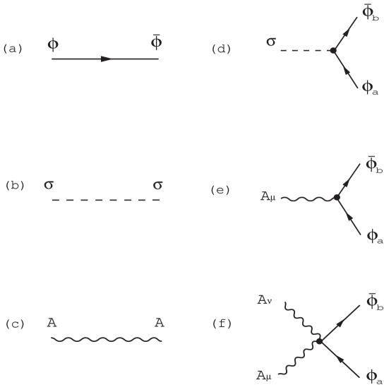
Fig. 12: Graphical representation of the large $N$ expansion in the $CP^{N-1}$ model. The propagators are as follows: (a) $\phi$ propagtor, $\delta_{ab}(p^{2}+m^{2})^{-1}$; (b) $\sigma$ propagator, $\mathchar 28928\relax(p)^{-1}$; (c) $A_{\mu}$ propagator, $\left(\delta_{\mu\nu}-{p_{\mu}p_{\nu}\over p^{2}}\right)\left[(p^{2}+4m^{2})\tilde{\mathchar 28928\relax}(p)-{1\over\pi}\right]^{-1}$. The vertices are as follows: (d) $\sigma\phi_{a}\bar{\phi}_{b}$ vertex (${i\over\sqrt{N}}\delta_{ab}$); (e) $A_{\mu}\phi_{a}\bar{\phi}_{b}$ vertex (${-1\over\sqrt{N}}\delta_{ab}(p_{\mu}+p_{\mu}^{\prime})$); (f) $A_{\mu}A_{\nu}\phi_{a}\bar{\phi}_{b}$ vertex (${-1\over N}\delta_{ab}\delta_{\mu\nu}$).

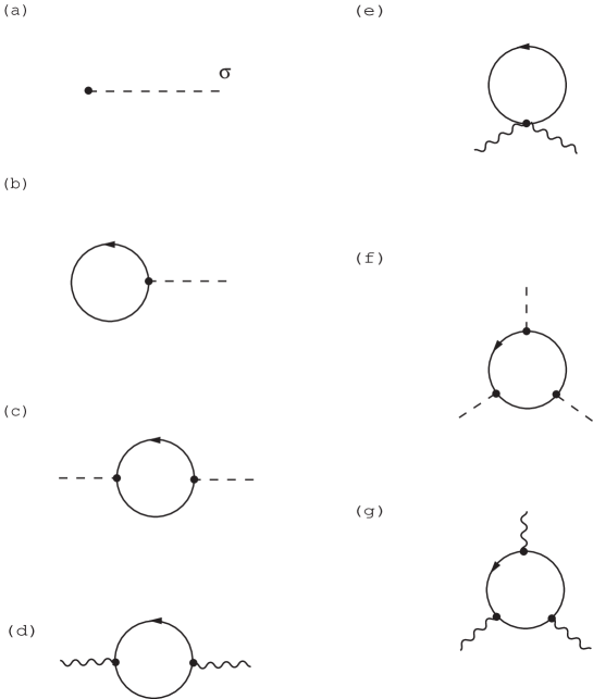
Fig. 13: Examples of Feynmann diagrams. (a) and (b) are tadpole diagrams of order $N^{1/2}$. (c),(d) and (e) are vacuum polarization diagrams of order $N^{0}$. (f) and (g) are order $N^{-1/2}$ diagrams.

First, the order $N^{1/2}$ term corresponds to the diagrams (a) and (b) in Fig. 13:

$$S^{(1)}={i\over g_{0}^{2}}\int d^{2}x\sigma(x)-i{\rm Tr}[(-\partial^{2}+m^{2})^{-1}\sigma]$$ (D.12)

$$=i\tilde{\sigma}(0)\left[{1\over g_{0}^{2}}-\int{d^{2}q\over(2\pi)^{2}}{1\over q^{2}+m^{2}}\right],$$ (D.13)

where we have used the Fourier transformation

$$\tilde{\sigma}(p)=\int d^{2}xe^{-ipx}\sigma(x).$$ (D.14)

The integral in (D.13) is ultraviolet divergent. It can be regularized by introducing the cutoff $\mathchar 28931\relax$. The saddle point condition $S^{(1)}=0$ requires the bare coupling constant $g_{0}$ to vary with the cutoff $\mathchar 28931\relax$ according to

$${1\over g_{0}^{2}(\mathchar 28931\relax)}={1\over 4\pi}\ln{\mathchar 28931\relax^{2}\over m^{2}}.$$ (D.15)

In other words, if the bare coupling $g_{0}$ varies with respect to the cutoff according to

$${1\over g_{0}^{2}(\mathchar 28931\relax)}-{1\over g_{R}^{2}(\mu)}={1\over 4\pi}\ln{\mathchar 28931\relax^{2}\over\mu^{2}},$$ (D.16)

the divergences cancel in $S^{(1)}$. This implies the asymptotic freedom of the $CP^{N-1}$ model. Imposing the condition $S^{(1)}=0$, therefore, we obtain

$$m^{2}=\mu^{2}\exp\left[-{4\pi\over g_{R}^{2}(\mu)}\right].$$ (D.17)

Next, the order $N^{0}$ term corresponds to the diagrams (c),(d) and (e) in Fig. 13:

$$S^{(2)}={1\over 2}\int d^{2}x\int d^{2}y[\sigma(x)\mathchar 28928\relax(x,y)\sigma(y)+A_{\mu}(x)\mathchar 28928\relax_{\mu\nu}(x,y)A_{\nu}(y)],$$ (D.18)

where the Fourier transformation of $\mathchar 28928\relax(x,y)$ and $\mathchar 28928\relax_{\mu\nu}(x,y)$ are respectively given by (see Fig. 13)

$$\tilde{\mathchar 28928\relax}(p) = \int{d^{2}q\over(2\pi)^{2}}{1\over(p^{2}+m^{2})((p+q)^{2}+m^{2})}$$ (D.19)

$$= {1\over 2\pi}{1\over\sqrt{p^{2}(p^{2}+4m^{2})}}\ln{\sqrt{p^{2}+4m^{2}}+\sqrt{p^{2}}\over\sqrt{p^{2}+4m^{2}}-\sqrt{p^{2}}},$$

and

$$\tilde{\mathchar 28928\relax}_{\mu\nu}(p) = 2\delta_{\mu\nu}\int{d^{2}q\over(2\pi)^{2}}{1\over q^{2}+m^{2}}-\int{d^{2}q\over(2\pi)^{2}}{(p_{\mu}+2q_{\mu})(p_{\nu}+2q_{\nu})\over(p^{2}+m^{2})((p+q)^{2}+m^{2})}$$ (D.20)

$$= \left(\delta_{\mu\nu}-{p_{\mu}p_{\nu}\over p^{2}}\right)\left[(p^{2}+4m^{2})\tilde{\mathchar 28928\relax}(p)-{1\over\pi}\right].$$

In the neighbourhood of $p^{2}=0$, we have

$$\tilde{\mathchar 28928\relax}(p)={1\over 24\pi m^{4}}(6m^{2}-p^{2})+O(p^{4}),\quad\tilde{\mathchar 28928\relax}_{\mu\nu}(p)=\left[{p^{2}\over 12\pi m^{2}}+O(p^{4})\right]\left(\delta_{\mu\nu}-{p_{\mu}p_{\nu}\over p^{2}}\right).$$

Thus we obtain the low-energy effective action,

$$S^{(2)}\cong\int d^{2}x{1\over 24\pi m^{4}}\sigma(x)\left(\partial^{2}+6m^{2}\right)\sigma(x)+\int d^{2}x{1\over 48\pi m^{2}}[\partial_{\mu}A_{\nu}(x)-\partial_{\nu}A_{\mu}(x)]^{2}.$$

It is important to note that the kinetic terms for the Lagrangian multiplier fields are generated. The field $\sigma$ becomes massive, while the field $A_{\mu}(=\sqrt{N}V_{\mu})$ is massless.

The line integral in the Wilson loop can be rewritten as

$$\oint_{C}d\xi_{\mu}V_{\mu}(\xi)=\int d^{2}zV_{\mu}(z)J_{\mu}(z)=:(V_{\mu},J_{\mu}),$$ (D.23)

where

$$J_{\mu}(z)=\oint_{C}d\xi_{\mu}\delta^{2}(z-\xi)=\epsilon_{\mu\nu}\partial_{\nu}\mathchar 28936\relax(z),\quad\mathchar 28936\relax(z)=\cases{1&($z\in S_{C}$)\cr 0&($z\notin S_{C}$)}.$$ (D.24)

Here $S_{C}$ is the area bounded by the loop $C$. Up to leading order, we can perform the Gaussian integration to obtain

$${\hbox{$\left\langle\vbox to0.0pt{}\right.\n@space$}}\exp\left[i\oint_{C}d\xi_{\mu}V_{\mu}(\xi)\right]{\hbox{$\left\rangle\vbox to0.0pt{}\right.\n@space$}}_{CP^{N-1}} \cong Z^{-1}[0,0,0]\int{\cal D}\sigma{\cal D}A_{\mu}e^{-S^{(2)}}\exp\left({i\over\sqrt{N}}(A_{\mu},J_{\mu})\right)$$ (D.25)

$$= {\rm const}\exp\left[-{1\over 2}{12\pi m^{2}\over N}(J_{\mu},\mathchar 28929\relax^{-1}J_{\mu})\right].$$

Thus we obtain the area law,

$${\hbox{$\left\langle\vbox to0.0pt{}\right.\n@space$}}\exp\left[i\oint_{C}d\xi_{\mu}V_{\mu}(\xi)\right]{\hbox{$\left\rangle\vbox to0.0pt{}\right.\n@space$}}_{CP^{N-1}}={\rm const}\exp\left[-{6\pi m^{2}\over N}|S_{C}|\right],$$ (D.26)

since $J={}^{*}d\mathchar 28936\relax$ and $\mathchar 28929\relax:=d\delta+\delta d$, and hence

$$(J_{\mu},\mathchar 28929\relax^{-1}J_{\mu}):=\int d^{2}x\int d^{2}yJ_{\mu}(x)\mathchar 28929\relax^{-1}(x,y)J_{\mu}(y)=(\mathchar 28936\relax,\mathchar 28936\relax)=|S_{C}|.$$ (D.27)

The dynamically generated gauge field $A_{\mu}$ produces a long-range force with a linear potential that confines the $\phi$s. Both global $SU(N)$ and local $U(1)$ symmetries are unbroken in two dimensions due to the Coleman theorem. In dimensions $D>2$, it has been shown [70] that there is a critical point $g_{c}$ such that for $g<g_{c}$ $SU(N)$ and $U(1)$ symmetries are broken, $\langle\phi_{a}\rangle\not=0$, while $\langle\sigma\rangle=0$. In this phase $\phi$ is regarded as the Nambu-Goldstone particle, since $m_{\phi}=0$. A massless vector pole exists in the propagator $\langle A_{\mu}(x)A_{\nu}(0)\rangle$.[71] For $g>g_{c}$, on ther other hand, the $SU(N)$ and $U(1)$ symmetries are exact, implying $\langle\phi_{a}\rangle=0$, and $\langle\sigma\rangle\not=0$. In this phase, $\phi$ is massive, $m_{\phi}=\langle\sigma\rangle$. For $D=2$, $g_{c}=0$. For more details on large $N$ results, see Refs.?, ?, ?, ?.

E Large N Estimation

If we write $n^{A}(x)$ in terms of the $CP^{N-1}$ variable $\phi_{a}(x)$ as

$$n^{A}(x)=\bar{\phi}_{a}(x)(T^{A})_{ab}\phi_{b}(x),$$ (E.1)

we obtain

$$n^{A}(x)n^{A}(y) = \bar{\phi}_{a}(x)(T^{A})_{ab}\phi_{b}(x)\bar{\phi}_{c}(y)(T^{A})_{cd}\phi_{d}(y)$$

$$= P_{ab}(x)P_{cd}(y)(T^{A})_{ab}(T^{A})_{cd}$$

$$= {1\over 2}\left[(\bar{\phi}(x)\cdot\phi(y))(\phi(x)\cdot\bar{\phi}(y))-{1\over N}(\bar{\phi}(x)\cdot\phi(x))(\bar{\phi}(y)\cdot\phi(y))\right],$$

where we have used

$$\sum_{A=1}^{N^{2}-1}(T^{A})_{ab}(T^{A})_{cd}={1\over 2}\left(\delta_{ad}\delta_{bc}-{1\over N}\delta_{ab}\delta_{cd}\right).$$ (E.3)

Hence we obtain

$${\bf n}(x)\cdot{\bf n}(x)=n^{A}(x)n^{A}(x)={1\over 2}\left[1-{1\over N}\right](\bar{\phi}(x)\cdot\phi(x))^{2}.$$ (E.4)

The contraint $\bar{\phi}(x)\cdot\phi(x)=1$ leads to ${\bf n}(x)\cdot{\bf n}(x)={1\over 2}\left[1-{1\over N}\right].$ The expectation value reads

$$2\langle n^{A}(x)n^{A}(y)\rangle = \langle(\bar{\phi}(x)\cdot\phi(y))(\phi(x)\cdot\bar{\phi}(y))\rangle-{1\over N}\langle|\phi(x)|^{2}|\phi(y)|^{2}\rangle.$$ (E.5)

The factorization in the large $N$ expansion leads to

$$2\langle n^{A}(x)n^{A}(y)\rangle \cong \langle\bar{\phi}(x)\cdot\phi(y)\rangle\langle\phi(x)\cdot\bar{\phi}(y)\rangle-{1\over N}\langle|\phi(x)|^{2}\rangle\langle|\phi(y)|^{2}\rangle,$$ (E.6)

$$= |\langle\bar{\phi}(x)\cdot\phi(y)\rangle|^{2}-{1\over N}\langle|\phi(x)|^{2}\rangle\langle|\phi(y)|^{2}\rangle.$$

The large $N$ expansion shows that the field $\phi$ becomes massive, so that the two-point function $\langle\bar{\phi}(x)\cdot\phi(y)\rangle$ exhibits exponential decay.

To leading order in the large $N$ expansion, the correlation function $G_{C}(x,y)$ defined by (9.32) in the $CP^{N-1}_{2}$ model reads

$$G_{C}(x,y)\cong\tilde{G}(x,y):=\left(\delta_{ad}\delta_{bc}-{1\over N}\delta_{ab}\delta_{cd}\right)\langle P_{ab}(x)P_{ba}(y)\rangle_{CP^{N-1}_{2}}.$$ (E.7)

Note that $P$ is a projection operator with the properties

$$P^{2}(x)=P(x),\quad{\rm tr}P(x)=1.$$ (E.8)

The composite operator $P$ is $U(1)$ gauge invariant. $SU(N)$ invariance implies that

$$\langle P_{ab}(x)\rangle=\langle\bar{\phi}_{a}(x)\phi_{b}(x)\rangle={1\over N}\delta_{ab}.$$ (E.9)

It is easy to show that

$$\tilde{G}(x,y) = \langle\bar{\phi}_{a}(x)\phi_{b}(x)\bar{\phi}_{b}(y)\phi_{a}(y)\rangle-{1\over N}$$ (E.10)

$$= \langle D^{2}(x,y)\rangle+{1\over N}\langle D(x,x)D(y,y)\rangle-{1\over N}$$

$$= \langle D^{2}(x,y)\rangle+{1\over N}\langle D(x,x)D(y,y)\rangle_{conn},$$

where $\langle D(x,x)\rangle=1$.

References

-
[1]
M. Gell-Mann,
Phys. Lett. 8 (1964), 214.
G. Zweig, CERN Rep. 8419/TH 412. -
[2]
C.N. Yang and R.L. Mills,
Phys. Rev. 96 (1954), 191.
R. Utiyama, Phys. Rev. 101 (1956), 1597.
R. Shaw, The problem of particle types and other contributions to the theory of elementary particles, Cambridge University Ph.D. thesis (unpublished). -
[3]
G. ’t Hooft,
in Conference on lagrangian field theory, Marseille,
1972 (unpublished).
D.J. Gross and F. Wilczek, Phys. Rev. Lett. 30 (1973), 1343.
H.D. Politzer, Phys. Rev. Lett. 30 (1973), 1346. - [4] K. Wilson, Phys. Rev. D10 (1974), 2445.
-
[5]
M. Creutz,
Phys. Rev. Lett. 45 (1980), 313
M. Creutz and K.J.M. Moriarty, Phys. Rev. D26 (1982), 2166. -
[6]
Y. Nambu,
Phys. Rev. D10 (1974), 4262.
G. ’t Hooft, in High Energy Physics, ed. by A. Zichichi (Editorice Compositori, Bologna, 1975).
S. Mandelstam, Phys. Report 23 (1976), 245. - [7] A.M. Polyakov, Phys. Lett. B59 (1975), 82; Nucl. Phys. B120 (1977), 429; Gauge fields and strings (Harwood Academic Publishers, London, 1987).
- [8] N. Seiberg and E. Witten, hep-th/9407087, Nucl. Phys. B426 (1994), 19.
-
[9]
T. Suzuki,
hep-lat/9506016.
R.W. Haymaker, hep-lat/9510035.
A. DiGiacomo, hep-th/9603029.
M.I. Polikarpov, hep-lat/9609020.
M.N. Chernodub and M.I. Polikarpov, hep-th/9710205.
G.S. Bali, hep-ph/9809351. -
[10]
G. ’t Hooft,
Nucl. Phys. B190 (1981), 455.
A. Kronfeld, G. Schierholz and U.-J. Wiese, Nucl. Phys. B293 (1987), 461.
A. Kronfeld, M. Laursen, G. Schierholz and U.-J. Wiese, Phys. Lett. B198 (1987), 516. - [11] K.-I. Kondo and Y. Taira, hep-th/9906129, Mod. Phys. Lett. A13 (2000), 366.
- [12] K.-I. Kondo, hep-th/9709109, Phys. Rev. D57 (1998), 7467
- [13] K.-I. Kondo, hep-th/9801024, Phys. Rev. D58 (1998), 105019.
- [14] K.-I. Kondo, hep-th/9803133, Phys. Rev. D58 (1998), 085013.
- [15] K.-I. Kondo, hep-th/9805153, Phys. Rev. D58 (1998), 105016.
- [16] K.-I. Kondo, hep-th/9810167, Phys. Lett. B455 (1999), 251.
- [17] K.-I. Kondo, hep-th/9904045, Intern. J. Mod. Phys. A, to be published.
- [18] M. Faber, J. Greensite and S. Olejnik, hep-lat/9807008; hep-lat/9710039, Phys. Rev. D57 (1998), 2603.
- [19] R. Wensley, Poster at Lattice 99, Pisa, Italy.
-
[20]
M.B. Halpern,
Phys. Rev. D19 (1979), 517.
N.E. Bralic, Phys. Rev. D22 (1980), 3090.
I.Ya. Aref’eva, Theor. Math. Phys. 43 (1980), 353
Yu.A. Simonov, Yad. Fiz. 50 (1989), 213 [Sov. J. Nucl. Phys. 50 (1989), 134].
B. Broda, Phys. Lett. B262 (1991), 288.
B. Broda, J. Math. Phys. 33 (1992), 1511.
F.A. Lunev, hep-th/9609166, Nucl. Phys. B494 (1997), 433.
M. Hirayama and S. Matsubara, hep-th/9712120, Prog. Theor. Phys. 99 (1998), 691;
M. Hirayama, M. Kanno, M. Ueno and H. Yamakoshi, hep-th/9806098, Prog. Theor. Phys. 100 (1998), 817.
R.L. Karp, F. Mansouri, J.S. Rno, hep-th/9903221; hep-th/9910173, J. Math. Phys. 40 (1999), 6033. - [21] D.I. Diakonov and V.Yu. Petrov, Phys. Lett. B224 (1989), 131; hep-th/9606104.
- [22] D.H. Feng, R. Gilmore and W.-M. Zhang, Rev. Mod. Phys. 62 (1990), 867.
-
[23]
A.M. Perelomov,
Phys. Report 146 (1987), 135.
A.M. Perelomov and M.C. Prati, Nucl. Phys. B258 (1985), 647. - [24] M.-H. Kim and P. Oh, hep-th/9504001.
- [25] Z.F. Ezawa and A. Iwasaki, Phys. Rev. D25 (1982), 2681.
- [26] T. Suzuki and I. Yotsuyanagi, Phys. Rev. D42 (1990), 4257.
-
[27]
G. ’t Hooft,
Nucl. Phys. B79 (1974), 276.
A.M. Polyakov, JETP Lett. 20 (1974), 194. - [28] L.G. Yaffe, Rev. Mod. Phys. 54 (1982), 407.
- [29] S. Coleman, 1/N in Aspect of Symmetry (Cambridge Univ. Press, New York, 1985) .
- [30] S.R. Das, Rev. Mod. Phys. 59 (1987), 235.
- [31] P. Rossi, M. Campostrini and E. Vicari, Phys. Reports 302 (1998), 143.
- [32] G. ’t Hooft, Nucl. Phys. B72 (1974), 461.
- [33] K. Ueno, Introduction to algebraic geometry (in Japanese), (Iwanami, Tokyo, 1995).
-
[34]
M.A.B. Beg and H. Ruegg,
J. Math. Phys. 6 (1965), 677.
E. Chacon and M. Moshinsky, Phys. Lett. 23 (1966), 567.
T.J. Nelson, J. Math. Phys. 8 (1967), 857.
D.F. Holland, J. Math. Phys. 10 (1969), 531. - [35] M. Nakahara, Geometry, Topology and Physics, (IOP, Bristol, 1990).
- [36] M.B. Green, J.H. Schwarz and E. Witten, Sueprstring theory, Vol. 2: loop amplitudes, anomalies phenomenology (Cambridge Univ. Press, Cambridge, 1987).
- [37] H. Georgi, Lie algebras in particle physics, from isospin to unified theories (Benjamin/Cummings, London, 1982).
- [38] R.F. Picken, J. Math. Phys. 31 (1990), 616.
- [39] D.P. Zelobenko, Compact Lie groups and their representations (AMS, Providence, 1973).
- [40] A. Perelomov, Generalized coherent states and their applications (Springer, New York, 1986).
- [41] F. Wilczek and A. Zee, Phys. Rev. Lett. 52 (1984), 2111.
- [42] K.-I. Kondo and T. Shinohara, hep-th/0004158, Phys. Lett. B491 (2000), 263
- [43] K.-I. Kondo, in preparation.
- [44] L. Faddeev and A.J. Niemi, hep-th/9807069,; Phys. Rev. Lett. 82 (1999), 1624; hep-th/9812090, Phys. Lett. B449 (1999), 214.
- [45] P.A.M. Dirac, Proc. Roy. Soc. London A133 (1931), 60; Phys. Rev. 74 (1948), 817.
- [46] T.T. Wu and C.N. Yang, Phys. Rev. D12 (1975), 3845; Nucl. Phys. B107 (1976), 365.
- [47] M. Hirayama and M. Ueno, hep-th/9907063, Prog. Theor. Phys. 103 (2000), 151.
- [48] E.J. Weinberg, Massless and massive monopoles carrying nonabelian magnetic charges, hep-th/9610065.
- [49] A. Sinha, Phys. Rev. D14 (2016), 1976
- [50] M. Quandt and H. Reinhardt, hep-th/9707185, Int. J. Mod. Phys. A13 (1998), 4049.
- [51] K.-I. Kondo and T. Shinohara, Renormalizable Abelian-projected effective gauge theory derived from Quantum Chromodynamics, CHIBA-EP-121, hep-th/0005125, and paper in preparation.
- [52] K. Amemiya and H. Suganuma, Phys. Rev. D60 (1999), 114509.
- [53] M. Lüscher, Phys. Lett. B78 (1978), 465.
- [54] D.J. Gross, Nucl. Phys. B132 (1978), 439.
-
[55]
B. Berg and M. Lüscher,
Commun. Math. Phys. 69 (1979), 57.
V.A. Fateev, I.V. Frolov and A.S. Schwarz, Nucl. Phys. B154 (1979), 1; Sov. J. Nucl. Phys. 30 (1979), 590.
A.P. Bukhvostov and L.N. Lipatov, Nucl. Phys. B180 (1981), 116
P.G. Silvestrov, Sov. J. Nucl. Phys. 51 (1990), 1121. - [56] A. D’adda, P. di Vecchia and M. Lüscher, Nucl. Phys. B146 (1978), 63.
- [57] A. D’adda, P. di Vecchia and M. Lüscher, Nucl. Phys. B152 (1979), 125.
- [58] E. Witten, Nucl. Phys. B149 (1979), 285.
- [59] G. Münster, Phys. Lett. B118 (1982), 380. Nucl. Phys. B218 (1983), 1.
- [60] M. Campostrini and P. Rossi, Phys. Rev. D45 (1992), 618; Phys. Lett. B272 (1991), 305.
-
[61]
D. Gross,
hep-th/9212149,
Nucl. Phys. B400 (1993), 161.
D. Gross and W. Taylor IV, hep-th/9301068, Nucl. Phys. B400 (1993), 181; hep-th/9303046, Nucl. Phys. B403 (1993), 395. - [62] J.B. Kogut, Rev. Mod. Phys. 55 (1983), 775.
- [63] J. Schwinger, Phys. Lett. B24 (1967), 473, Phys. Rev. 167 (1968), 1432
- [64] K.-I. Kondo and Y. Taira, Nucl. Phys. Proc. Suppl. 83, 497 (2000).
- [65] A.M. Polyakov, hep-th/9607049, Nucl. Phys. B486 (1997), 23; hep-th/971002, Nucl. Phys. B Proc. Suppl. 68 (1998), 1; hep-th/9809057, Int. J. Mod. Phys. A14 (1999), 645.
- [66] M. Stone, Nucl. Phys. B152 (1979), 97.
- [67] H.E. Haber, I. Hinchliffe and E. Rabinovici, Nucl. Phys. B172 (1980), 458.
- [68] A.J. Macfarlane, Nucl. Phys. B152 (1979), 145.
- [69] W.A. Bardeen, B.W. Lee and R.E. Shrock, Phys. Rev. D14 (1976), 985.
- [70] I.Ya. Arefeva and S.I. Azakov, Nucl. Phys. B162 (1980), 298.
-
[71]
T. Kugo and P. Townsend,
Phys. Lett. B101 (1981), 82.
S. Weinberg and E. Witten, Phys. Lett. B96 (1980), 59.
T. Kugo, Phys. Lett. B109 (1982), 205.
T. Kugo, H. Terao and S. Uehara, Prog. Theor. Phys. Suppl. 85 (1985), 122.
T. Kugo, Soryushiron Kenkyu (Kyoto) 71, E78-90 (1985); Prog. Theor. Phys. 66 (1981), 2249.
M. Bando, T. Kugo and K. Yamawaki, Phys. Reports 164 (1988), 217. - [72] Y. Imry and S.K. Ma, Phys. Rev. Lett. 35 (1975), 1399.
-
[73]
J.Z. Imbrie,
Commun. Math. Phys. 98 (1985), 145.
J. Bricmont and A. Kupiainen, Phys. Rev. Lett. 59 (1987), 1829. - [74] J. Cardy, Phys. Lett. B125 (1983), 470.
- [75] A. Klein and J. Perez, Phys. Lett. B125 (1983), 473.
- [76] A. Klein, L. Landau and J. Perez, Commun. Math. Phys. 94 (1984), 459.
- [77] G. Parisi and N. Sourlas, Nucl. Phys. B206 (1982), 321
- [78] J. Zinn-Justin, Chapter 16: Slavnov-Taylor and BRS symmetry. Stochastic field equations, in Quantum Field Theory and Critical Phenomena (Oxford Univ. Press, 1993).
- [79] K. Fujikawa, Nucl. Phys. B223 (1983), 218.
- [80] F. Bruckmann, T. Heinzl, T. Tok and A. Wipf, Instantons and Gribov copies in the maximally Abelian gauge, hep-th/0001175.