UCLA/99/TEP/46 SU-ITP-99-51 hep-th/99mmnnn

The Operator Product Expansion of ${\cal N}=4$ SYM

and the 4–point Functions of Supergravity

Eric D’Hoker${}^{\,a}$, Samir D. Mathur${}^{\,b}$,

Alec Matusis${}^{\,c}$, Leonardo Rastelli${}^{\,d,}$

^a Department of Physics

University of California, Los Angeles, CA 90095

^b Department of Physics

Ohio State University, Columbus OH 43210

^c Department of Physics

Stanford University, Stanford, CA 94305

^d Center for Theoretical Physics

Massachusetts Institute of Technology, Cambridge, MA 02139

We give a detailed Operator Product Expansion interpretation of the results for conformal 4–point functions computed from supergravity through the AdS/CFT duality. We show that for an arbitrary scalar exchange in $AdS_{d+1}$ all the power–singular terms in the direct channel limit (and only these terms) exactly match the corresponding contributions to the OPE of the operator dual to the exchanged bulk field and of its conformal descendents. The leading logarithmic singularities in the 4–point functions of protected ${\cal N}=4$ super–Yang Mills operators (computed from IIB supergravity on $AdS_{5}\times S^{5}$) are interpreted as $O(\frac{1}{N^{2}})$ renormalization effects of the double–trace products appearing in the OPE. Applied to the 4–point functions of the operators ${\cal O}_{\phi}\sim({\rm tr}F^{2}+\dots)$ and ${\cal O}_{C}\sim({\rm tr}F\tilde{F}+\dots)$, this analysis leads to the prediction that the double–trace composites $[{\cal O}_{\phi}{\cal O}_{C}]$ and $[{\cal O}_{\phi}{\cal O}_{\phi}-{\cal O}_{C}{\cal O}_{C}]$ have anomalous dimension $-\frac{16}{N^{2}}$ in the large $N$, large $g_{YM}^{2}N$ limit. We describe a geometric picture of the OPE in the dual gravitational theory, for both the power–singular terms and the leading logarithms. We comment on several possible extensions of our results.

1 Introduction

The study of 4–dimensional Conformal Field Theories is an old and important topic. The AdS/CFT correspondence [1, 2] provides new powerful tools to address this problem. Difficult dynamical questions about the strong coupling behavior of the CFT are answered by perturbative computations in Anti de Sitter supergravity. A natural set of questions concerns the nature of the Operator Product Expansion of the CFT at strong coupling. Thanks to the AdS/CFT duality, we can now answer some of these questions.

The prime example of an exactly conformal 4–dimensional field theory, namely the ${\cal N}=4$ Super–Yang Mills theory with gauge group $SU(N)$, is dual [1] to Type IIB string theory on $AdS_{5}\times S^{5}$, with $N$ units of 5–form flux and compactification radius $R^{2}=\alpha^{\prime}(g_{YM}^{2}N)^{\frac{1}{2}}$. For large $N$ and large ’t Hooft coupling $\lambda\equiv g_{YM}^{2}N$ the dual string theory is approximated by weakly coupled supergravity in $AdS_{5}$ background. Since the 5–dimensional Newton constant $G_{5}\sim R^{3}/N^{2}$, the perturbative expansion in supergravity corresponds to the $1/N$ expansion in the CFT. Correlation functions of local operators of the CFT belonging to short multiplets of the superconformal algebra are given for $N\rightarrow\infty$, $\lambda\rightarrow\infty$ by supergravity amplitudes according to the prescription of [4, 5]. While the supergravity results for 2– and 3–point functions of chiral operators [6]–[9] have been found to agree with the free field approximation, giving strong evidence for the existence of non–renormalization theorems [10]–[12], 4–point functions [13]–[26] certainly contain some non–trivial dynamical information.

The 4–point functions of the operators ${\cal O}_{\phi}$ and ${\cal O}_{C}$ dual to the dilaton and axion fields were obtained in [22] through a supergravity computation, and expressed as very explicit series expansions in terms of two conformal invariant variables. The fundamental fields of the ${\cal N}=4$ theory are the gauge boson $A_{\mu}$, 4 Majorana fermions $\lambda^{a}$ and 6 real scalars $X^{i}$, all in the adjoint representation of the gauge group $SU(N)$. The operators ${\cal O}_{\phi}$ and ${\cal O}_{C}$ are the exactly marginal operators that correspond to changing the gauge coupling and the theta angle of the theory. In other terms the SYM Lagrangian has the form ${\cal L}\sim\frac{1}{g_{YM}^{2}}\,{\cal O}_{\phi}+\frac{\theta}{8\pi^{2}}\,{\cal O}_{C}$. It is convenient to define operators that have unit–normalized 2–point functions, $\hat{\cal O}_{\phi}\sim\frac{1}{N}\,{\cal O}_{\phi}\sim\frac{1}{N}\,{\rm tr}(F^{2}+\dots)$ and $\hat{\cal O}_{C}\sim\frac{1}{N}\,{\cal O}_{C}\sim\frac{1}{N}\,{\rm tr}(F\tilde{F}+\dots)$.

The computation of the axion–dilaton 4–point functions required the sum of several supergravity diagrams, weighted by the appropriate couplings in the Type IIB action on $AdS_{5}\times S^{5}$,

$$S=\frac{1}{2\kappa_{5}^{2}}\int_{AdS_{5}}d^{5}z\,\sqrt{g}\;\left(-{\cal R}+\Lambda+\frac{1}{2}\,g^{\mu\nu}\partial_{\mu}\phi\partial_{\nu}\phi+\frac{1}{2}\,e^{2\phi}\,g^{\mu\nu}\partial_{\mu}C\partial_{\nu}C\right).$$ (1.1)

Besides these ‘complete’ dilaton–axion 4–point functions, explicit results for arbitrary supergravity exchange diagrams involving massive scalars, massive vectors and massless gravitons are also available [23]. In the present paper we give a detailed OPE interpretation of some of these results, and obtain new predictions for the strong coupling behavior of the ${\cal N}=4$ SYM theory. The fact that the 5d supergravity amplitudes can be consistently interpreted in terms of a 4d local OPE is by itself quite remarkable, and constitutes a strong test of the AdS/CFT duality.

Let us introduce the main issues from the field theory viewpoint. By considering the limit of a 4–point function as the operator locations become pairwise close (take a ‘t–channel’ limit $x_{13}\equiv|\vec{x}_{1}-\vec{x}_{3}|\rightarrow 0$ and $x_{24}\equiv|\vec{x}_{2}-\vec{x}_{4}|\rightarrow 0$), we expect a double OPE expansion to hold:

$$\langle{\cal O}_{1}(\vec{x}_{1}){\cal O}_{2}(\vec{x}_{2}){\cal O}_{3}(\vec{x}_{3}){\cal O}_{4}(\vec{x}_{4})\rangle=\\ \sum_{n,m}\,\frac{\alpha_{n}\;\langle{\cal O}_{n}(\vec{x}_{1}){\cal O}_{m}(\vec{x}_{2})\rangle\;\beta_{m}}{(x_{13})^{\Delta_{1}+\Delta_{3}-\Delta_{m}}(x_{24})^{\Delta_{2}+\Delta_{4}-\Delta_{n}}}\,,$$ (1.2)

at least as an asymptotic series, and hopefully with a finite radius of convergence in $x_{13}$ and $x_{24}$. For simplicity we have suppressed all Lorentz and flavor structures and generically denoted by $\{{\cal O}_{n}\}$ the set of primary operators ${\cal O}_{p}$ and their conformal descendents $\bigtriangledown^{k}{\cal O}_{p}$. Let us take the operators in the 4–point function to be ‘single–trace’ chiral primaries ${\rm tr}(X^{(i_{1}}\dots X^{i_{k})})$ or any of their superconformal descendents, such as ${\cal O}_{\phi}\sim{\rm tr}(F^{2}+\dots)$. These operators belong to short representations of the superconformal algebra and their dimensions do not receive quantum corrections. On purely field–theoretic grounds, we expect that all the operators allowed by selection rules (most of which are not chiral) can contribute as intermediate states to the r.h.s. of (1.2).

The AdS/CFT duality makes the interesting prediction that the non–chiral operators of the SYM theory actually fall into two classes, which behave very differently at strong coupling:

• Operators dual to string states, like for example the Konishi operator ${\rm tr}X^{i}X^{i}$, whose dimensions become very large in the strong coupling limit (as $\sim\lambda^{\frac{1}{4}}$);

• Multi–trace operators obtained by taking (suitably regulated) products of single–trace chiral operators at the same point, like for example the normal–ordered product $[{\cal O}_{\phi}{\cal O}_{\phi}]$. These operators are dual to multi–particle supergravity states.

Since in the limit of large $N$, large $\lambda$ the dual supergravity description is weakly coupled, the dimension of a multi–particle state is approximately the sum of the dimensions of the single–particle (single–trace in SYM language) constituents, with small corrections of order $G_{5}\sim 1/N^{2}$ due to gravitational interactions. From a perturbative analysis in the SYM theory it is not hard to show (see Section 4.2) that for large $N$ and small $\lambda$ the anomalous dimension of an operator like $[{\cal O}_{\phi}{\cal O}_{\phi}]$ is of the form $\sim\frac{1}{N^{2}}f(\lambda)+O(\frac{1}{N^{4}})$, where $f(\lambda)$ can be computed as a perturbative series $f(\lambda)=\sum_{k\geq 1}a_{k}\lambda^{k}$. The AdS/CFT duality then predicts that as $\lambda\rightarrow\infty$ the function $f(\lambda)$ saturates to a finite value.

A non–trivial issue is whether in the double OPE intepretation of the supergravity amplitudes one can find any remnant of the non–chiral operators corresponding to string states. In fact, although these operators acquire a large anomalous dimension as $\lambda\rightarrow\infty$, an infinite number of them is exchanged in the r.h.s. of (1.2) for any finite $\lambda$, and one may worry about a possible non–uniformity of the limit. On the contrary, our analysis will lend support to the idea that as $\lambda\rightarrow\infty$ the string states consistently decouple.

Since each single–trace chiral operator ${\cal O}$ of the SYM theory is dual to some Kaluza–Klein mode $\phi$ of supergravity, there appears to be a 1–1 correspondence between supergravity diagrams in which $\phi$ is exchanged in the ‘t–channel’ (that is, the bulk–to–bulk $\phi$ propagators joins the pairs ${\cal O}_{1}{\cal O}_{3}$ and ${\cal O}_{2}{\cal O}_{4}$, see Fig.1) and the contribution to the double OPE (1.2) of the operator $\cal O$ and its conformal descendents $\bigtriangledown^{k}{\cal O}$. In Section 2 we prove a general theorem: for any scalar exchange in $AdS_{d+1}$ all the singular terms $O(\frac{1}{x_{13}^{n}})$ (and only these terms) exactly match the corresponding contributions of the conformal block $\{\bigtriangledown^{k}{\cal O}\}$ to the double OPE (1.2) of the $d$–dimensional boundary CFT. We believe that a similar theorem must hold for exchanges of arbitrary spin. The correspondence between supergravity exchanges and ‘conformal partial waves’ breaks down precisely when the double–trace operator $[{\cal O}_{1}{\cal O}_{3}]$, which has dimension $\Delta_{1}+\Delta_{3}+O(1/N^{2})$, starts contributing to the OPE. This result implies that as $\lambda\rightarrow\infty$ the singular part of the OPE of two chiral SYM operators is entirely given by other chiral operators and their multi–trace products. This is of course consistent with the expectation that non–chiral operators corresponding to string states have a large dimension in this limit.

A generic feature of supergravity 4–point amplitudes is that their asymptotic expansions contain logarithmic terms. For example, a ‘t–channel’ exchange diagram (Fig.1) contains as $x_{13}\rightarrow 0$ a logarithmic singularity of the form $\frac{1}{x_{12}^{2\Delta_{1}+2\Delta_{2}}}\log\left(\frac{x_{13}x_{24}}{x_{12}x_{34}}\right)$, as well as a whole series of regular terms $x_{13}^{n}\log(x_{13})$. (All these terms are subleading with respect to the power singularities $O(\frac{1}{x_{13}^{k}})$ discussed above. The expansion of the same diagram in the limit $x_{12}\rightarrow 0$ contains instead no power singularities, and the logarithmic term is leading.) This logarithmic behavior may appear puzzling in a unitary CFT. However, as stressed to us by Witten early in this work, logs naturally arise in the perturbative expansion of a CFT from anomalous dimensions and operator mixing.

Section 3 of the paper is devoted to a general discussion of the logarithmic behavior of CFT’s. The difference between logs that arise in a pertubative expansion of a unitary theory and the ‘intrinsic logs’ of a non–unitary theory is emphasized. In our case the perturbative parameter is $1/N$. As already noted, we expect operators like $[{\cal O}_{\phi}{\cal O}_{\phi}]$ to have anomalous dimensions of order $O(\frac{1}{N^{2}})$. The logs in the supergravity 4–point functions arise indeed at the correct order and with the right structure to be interpreted as $O(\frac{1}{N^{2}})$ renormalization effects of the double–trace composites produced in the OPE of two chiral operators.

In Section 4, we perform a careful analysis of the leading logarithmic terms in the supergravity correlators $\langle{\cal O}_{\phi}{\cal O}_{\phi}{\cal O}_{\phi}{\cal O}_{\phi}\rangle$ and $\langle{\cal O}_{\phi}{\cal O}_{C}{\cal O}_{\phi}{\cal O}_{C}\rangle$. In order to reproduce the structure of the supergravity logs it is crucial to take into account the mixing between operators with the same quantum numbers, like $[{\cal O}_{\phi}{\cal O}_{\phi}]$ and $[{\cal O}_{C}{\cal O}_{C}]$. This analysis leads to the prediction of the strong coupling values of the anomalous dimensions of the operators $[{\cal O}_{\phi}{\cal O}_{C}]$ and $[{\cal O}_{\phi}{\cal O}_{\phi}-{\cal O}_{C}{\cal O}_{C}]$, which are the only two operators with the maximal $U_{Y}(1)$ charge $|Y|=4$ and thus cannot mix with any other operator of approximate dimension 8.

In Section 5 we present our conclusions and propose some avenues for future research.

2 Supergravity Exchanges versus OPE: Power Singularities

                                                                                                                                                          

Figure 1: Scalar exchange in the ‘t–channel’.

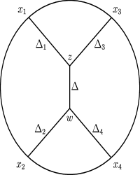
There is an intriguing relation [13] [14] between supergravity exchange diagrams and ‘conformal partial waves’. A conformal partial wave is the contribution to the double OPE representation (1.2) of a full conformal block, which consists of a given primary operator ${\cal O}_{p}$ and all its conformal descendents $\bigtriangledown^{k}{\cal O}_{p}$. Let us take the external operators ${\cal O}_{i}$ in the l.h.s. of (1.2) to be single–trace, chiral SYM operators and let us consider the partial waves in which the intermediate primaries are also single–trace and chiral. These are the operators which are in 1–1 correspondence with the single–particle Kaluza–Klein states of supergravity. It is then clear that for each such conformal partial wave one can draw a related supergravity diagram, in which the dual KK mode is exchanged in the bulk, see Fig.1.

Here we wish to compare supergravity scalar exchange diagrams in $AdS_{d+1}$ with conformal partial waves in $d$–dimensional CFT’s. We shall find that for a given partial wave all the singular terms in the OPE are exactly reproduced by the corresponding supergravity exchange. However the higher order terms are different.

The conformal partial wave for an intermediate scalar primary is an old result [35, 36]. Consider for simplicity the 4–point function of scalar operator ${\cal O}_{i}$ with pairwise equal dimensions ($\Delta_{1}=\Delta_{3}$, $\Delta_{2}=\Delta_{4}$). Introducing the conformal invariant variables

$$s\equiv\frac{1}{2}\frac{x_{13}^{2}x_{24}^{2}}{x_{12}^{2}x_{34}^{2}+x_{14}^{2}x_{23}^{2}}\,,\qquad\qquad t\equiv\frac{x_{12}^{2}x_{34}^{2}-x_{14}^{2}x_{23}^{2}}{x_{12}^{2}x_{34}^{2}+x_{14}^{2}x_{23}^{2}}\,.$$ (2.1)

the contribution from an intermediate operator ${\cal O}_{\Delta}$ and its conformal descendents can be written as (see Appendix A for the conversion from the form in [36] to our notations):

$$\langle{\cal O}_{1}(x_{1}){\cal O}_{2}(x_{2}){\cal O}_{3}(x_{3}){\cal O}_{4}(x_{4})\rangle_{0} = {1\over x_{13}^{2\Delta_{1}}x_{24}^{2\Delta_{2}}}\,2{\Gamma\left(\Delta\right)\Gamma\left(\Delta+1-{d\over 2}\right)\over\Gamma\left({\Delta\over 2}\right)^{4}}\,$$

$$\times \sum_{n=0}^{\infty}s^{{\Delta\over 2}+n}\,a_{{\Delta\over 2}+n-1}(t){\Gamma\left({\Delta\over 2}+n\right)^{2}\over\Gamma\left(n+\Delta-{d\over 2}+1\right)\,n!}\,,$$

where

$$a_{k}(t)=\sqrt{\pi}{\Gamma(k+1)\over\Gamma\left(k+{3\over 2}\right)}\,F\left({k+1\over 2},{k\over 2}+1;k+{3\over 2};t^{2}\right).$$ (2.3)

Here all operators are normalized to have unit two–point functions and the correlators $\langle{\cal O}_{1}{\cal O}_{3}{\cal O}_{\Delta}\rangle$ and $\langle{\cal O}_{2}{\cal O}_{4}{\cal O}_{\Delta}\rangle$ are also assumed to have coefficient 1. Observe that the singular terms in the limit $x_{13}\rightarrow 0$ are given by $n\leq\Delta_{1}-\frac{\Delta}{2}-1$.

The supergravity ‘t–channel’ exchange diagram of Fig.1 in which the field $\phi$ dual to ${\cal O}$ propagates in the bulk can be expressed in a similar series expansion in terms of the variables $s$ and $t$ (see Appendix A for details). Let $\Delta_{1}\leq\Delta_{2}$. It is found that in the limit $x_{13}\rightarrow 0$ the terms containing power singularities $O(\frac{1}{x_{13}^{k}})$ are

$$\langle{\cal O}_{\Delta_{1}}{\cal O}_{\Delta_{2}}{\cal O}_{\Delta_{3}}{\cal O}_{\Delta_{4}}\rangle\bigg{|}_{\rm sing} = {1\over x_{13}^{2\Delta_{1}}x_{24}^{2\Delta_{2}}}\,2{\Gamma\left(\Delta\right)\Gamma\left(\Delta+1-{d\over 2}\right)\over\Gamma\left({\Delta\over 2}\right)^{4}}\,$$

$$\times \sum_{n=0}^{\Delta_{1}-\frac{\Delta}{2}-1}s^{{\Delta\over 2}+n}\,a_{{\Delta\over 2}+n-1}(t){\Gamma\left({\Delta\over 2}+n\right)^{2}\over\Gamma\left(n+\Delta-{d\over 2}+1\right)\,n!}\,,$$

in precise agreement with (2). The full series expansion of the supergravity diagram is however different from (2), for example logarithmic terms $\sim\log s$ arise at the first non–singular order. Taking the limit $x_{24}\rightarrow 0$ (keeping the condition $\Delta_{1}\leq\Delta_{2}$) one finds that not all singular powers $O(\frac{1}{x_{24}^{k}})$ match, but only the terms more singular than $O(\frac{1}{x_{24}^{2\Delta_{2}-2\Delta_{1}}})$. This is precisely the singularity expected from the contribution to the OPE of the double–trace operator $[{\cal O}_{1}{\cal O}_{3}]$, of approximate dimension $2\Delta_{1}$. Not surprisingly, the correspondence between conformal partial waves and AdS exchanges breaks down precisely when double–traces start to contribute.

We expect similar results for arbitrary spin exchange. Expressions for conformal partial waves for arbitrary spin can be found for example in [37]. The exchange supergravity diagrams for vectors of general mass and massless gravitons have been evaluated in [16, 22, 23], where it was also checked that the leading power singularity reproduced the contribution expected from OPE considerations (see (4.23) of [16] and Sec. 2.3 of [22]). It would be interesting to extend the comparison to all the subleading power–singular singular terms.

                                                                                                                                                          

Figure 2: Upper–half plane representation of an exchange integral in AdS space. In the limit $x_{1}\to x_{2}$ the $z$–integral is supported in a small ball (in coordinate units) close to the boundary point $x_{1}\approx x_{2}$.

This nice holographic behavior of the $AdS_{d+1}$ supergravity exchange diagrams (their power singularities match the $d$–dimensional conformal OPE) can also be understood in the following heuristic way [13]. The exchange amplitude is given by an integral over the two bulk interaction points $z$ and $w$

$$I=\int[dz][dw]K_{\Delta_{1}}(z,\vec{x}_{1})K_{\Delta_{3}}(z,\vec{x}_{3})G_{\Delta}(z,w)K_{\Delta_{2}}(w,\vec{x}_{2})K_{\Delta_{4}}(w,\vec{x}_{4})$$ (2.5)

where $K$ and $G$ stand for the boundary–to–bulk and bulk–to–bulk propagators, and $[dz],[dw]$ denote the invariant measures. Take for concreteness the upper–half plane representation of AdS

$$ds^{2}=\frac{1}{z_{0}^{2}}\left(dz_{0}^{2}+(d\vec{z})^{2}\right)\,.$$ (2.6)

Then $K_{\Delta}(z,\vec{x})\sim\left(\frac{z_{0}}{z_{0}^{2}+(\vec{z}-\vec{x})^{2}}\right)^{\Delta}$. It is easy to prove that as we let $\vec{x}_{1}\rightarrow\vec{x}_{3}$, the $z$–integral is dominated by a small coordinate region, $\left\{z\;\,{\it s.t.}\,\left[z_{0}^{2}+(\vec{z}-\vec{x}_{1})^{2}\right]\sim x_{13}^{2}\right\}$, which is approaching the insertion points on the AdS boundary of the two colliding operators ${\cal O}(\vec{x}_{1}){\cal O}(\vec{x}_{3})$ (see Fig.2). This is another example of the UV/IR connection: short distances in the field theory are probed by large distance physics in the AdS description. As $x_{13}\rightarrow 0$ we can then approximate

$$G_{\Delta}(z,w)\longrightarrow\frac{1}{2\Delta-d}\;z_{0}^{\Delta}K_{\Delta}(\vec{x}_{1},w)\,,$$ (2.7)

and we get the expected factorization of (2.5) into a trivial integral over $z$ and an integral over $w$ which defines the 3–point function $\langle{\cal O}_{\Delta}{\cal O}_{2}{\cal O}_{4}\rangle$:

$$I\longrightarrow\frac{1}{{x_{13}}^{\Delta_{1}+\Delta_{3}-\Delta}}\,\langle{\cal O}_{\Delta}(\vec{x}_{1}){\cal O}_{2}(\vec{x}_{2}){\cal O}_{4}(\vec{x}_{4})\rangle\,$$ (2.8)

(the numerical coefficients work out exactly). The replacement (2.7) gives a clear geometric equivalent, on the supergravity side, of the operator product expansion ${\cal O}_{1}(\vec{x}_{1}){\cal O}_{3}(\vec{x}_{3})\rightarrow x_{13}^{-\Delta_{1}-\Delta_{3}+\Delta}{\cal O}_{\Delta}(\vec{x}_{1})$. It is possible to compute the first few higher–order corrections to (2.7) and to match them exactly [13] with the singular contributions to the operator product ${\cal O}_{1}{\cal O}_{3}$ of the descendents $\bigtriangledown^{k}{\cal O}_{\Delta}$.

So far we have analyzed the power singularities in the ‘direct channel’ limit of an exchange graph, i.e. when we let approach together two operators that join to the same bulk interaction vertex ($x_{13}\rightarrow 0$ or $x_{24}\rightarrow 0$ in (2.5)). A given 4–point function is obtained by summing all the crossed–symmetric exchanges, as well as ‘quartic’ graphs (diagrams with a single bulk interaction vertex, equ.(A.5)). Thus in analyzing the singular behavior of a 4–point correlator we also need to consider the type of leading singularities that appear in quartic graphs, as well as in the ‘crossed channel’ limit of an exchange graph (for example $x_{12}\rightarrow 0$ in (2.5)). It turns out that these two cases (crossed exchanges and quartic) have the same qualitative behavior: as $x_{12}\rightarrow 0$, the leading asymptotic is $O(\frac{1}{x_{12}^{\Delta_{1}+\Delta_{2}-\Delta_{3}-\Delta_{4}}})$ if $\Delta_{1}+\Delta_{2}-\Delta_{3}-\Delta_{4}>0$ or $\log(x_{12})$ if $\Delta_{1}+\Delta_{2}-\Delta_{3}-\Delta_{4}=0$, and the limit is smooth if $\Delta_{1}+\Delta_{2}-\Delta_{3}-\Delta_{4}<0$. These are the singularities expected from the contribution to the operator product ${\cal O}_{1}{\cal O}_{2}$ of the composite operator $[{\cal O}_{3}{\cal O}_{4}]$, which has dimension $\Delta_{3}+\Delta_{4}$ in the large $N$ limit.

The results of this Section have a clear implication for the ${\cal N}=4$ SYM theory: in the limit of large $N$, large $\lambda$, the only singular terms in the product of two chiral operators are given by other chiral operators and their multi–trace products (and their first few conformal descendents).

3 On the Logarithmic Behavior of Conformal Field Theories

3.1 General analysis

Let us analyze the issue of logarithms in general, for an arbitrary CFT, before returning to the case of the ${\cal N}=4$ supersymmetric Yang–Mills in 4 dimensions. A CFT is characterized by the absence of any inherent length scale. Under quite general conditions one can argue that for primary operators of the conformal algebra the 2–point function is forced by conformal invariance to have the form

$$\langle{\cal O}(x_{1}){\cal O}(x_{2})\rangle={C\over|x_{1}-x_{2}|^{2\Delta}}$$ (3.1)

The power law on the r.h.s. is covariant under scale transformations: if we write $x=\mu x^{\prime}$, then the 2–point function will be left unchanged provided we also change the operators from ${\cal O}$ to ${\cal O}^{\prime}=\mu^{-\Delta}{\cal O}$.

One might imagine that a logarithmic dependence $\log{|x_{1}-x_{2}|\over L}$ would violate conformal invariance of the theory, since a length scale $L$ is needed to make the argument of the logarithm dimensionless. There exists however a class of 2d theories called logarithmic CFTs, where logarithms do arise. These theories will not be the focus of our interest later on, so we mention them now and then exclude them from the rest of the discussion below. In logarithmic CFTs the dilation operator cannot be diagonalised, but (in the simplest case) has a Jordan form instead on a pair of operators ${\cal O},\tilde{\cal O}$. The 2–point functions are of the form

$$\langle{\cal O}(z_{1}){\cal O}(z_{2})\rangle = 0$$

$$\langle\tilde{\cal O}(z_{1}){\cal O}(z_{2})\rangle = {1\over(z_{1}-z_{2})^{2\Delta}}$$ (3.2)

$$\langle\tilde{\cal O}(z_{1})\tilde{\cal O}(z_{2})\rangle = {1\over(z_{1}-z_{2})^{2\Delta}}\log{z_{1}-z_{2}\over Y}$$

(In the above we have considered only the holomorphic parts of the operators.) Under a dilation $z=\mu z^{\prime}$ we must not only rescale the fields but also implement a shift transformation: ${\cal O}^{\prime}=\mu^{-\Delta}{\cal O},~{}\tilde{\cal O}^{\prime}=\mu^{-\Delta}[\tilde{\cal O}+{1\over 2}\log(\mu){\cal O}]$. With this change of variables the correlators of the rescaled theory become identical to the original ones, and so the parameter $Y$ in (3.1) does not represent a fundamental length in the theory, but instead describes a certain choice for the operator $\tilde{\cal O}$ from the subspace of operators ${\cal O},\tilde{\cal O}$ of the same dimension.

These logarithmic CFTs are however not expected to be unitary. In a radial quantization the dilation operator is the Hamiltonian. In 2–d CFT’s the eigenvalues of the dilation operator on the plane map to the eigenvalues of the time translation operator on the cylinder, so in a unitary theory we expect that the dilation operator will be diagonalisable and will not have a nontrivial Jordan form. Our case of interest (the 4d ${\cal N}=4$ supersymmetric Yang-Mills theory) is a unitary theory, and we will assume in what follows that the dilation operator is diagonalisable on the space of fields. The analysis of the next section will confirm this assumption.

For unitary CFTs the 3–point function of primary fields also has a standard form which is fixed by conformal invariance

$$\langle{\cal O}_{1}(x_{1}){\cal O}_{2}(x_{2}){\cal O}_{3}(x_{3})\rangle={\gamma_{123}\over x_{12}^{\Delta_{1}+\Delta_{2}-\Delta_{3}}x_{23}^{\Delta_{2}+\Delta_{3}-\Delta_{1}}x_{13}^{\Delta_{1}+\Delta_{3}-\Delta_{2}}}$$ (3.3)

where $x_{ij}\equiv|x_{i}-x_{j}|$. 4–point functions are however not fixed in their functional form by conformal invariance, though they are restricted to be a function of two cross ratios

$$\langle{\cal O}_{1}(x_{1}){\cal O}_{2}(x_{2}){\cal O}_{3}(x_{3}){\cal O}_{4}(x_{4})\rangle={1\over x_{13}^{\Sigma_{13}-\Delta_{13}}x_{12}^{\Delta_{13}+\Delta_{24}}x_{14}^{\Delta_{13}-\Delta_{24}}x_{24}^{\Sigma_{24}-\Delta_{13}}}\;f(\rho,\eta)$$ (3.4)

$$\qquad\qquad\qquad\qquad\eta={x_{12}^{2}x_{34}^{2}\over x_{13}^{2}x_{24}^{2}},\quad\rho={x_{14}^{2}x_{23}^{2}\over x_{13}^{2}x_{24}^{2}}$$ (3.5)

where $\Sigma_{ij}=\Delta_{i}+\Delta_{j}$, $\Delta_{ij}=\Delta_{i}-\Delta_{j}$. One might imagine that the expansion of $f$ in say $\eta$ would in general contain a logarithm:

$$f(\eta,\rho)=\dots+f_{-1}(\rho)\eta^{-1}+f_{0}(\rho)+\tilde{f}_{0}(\rho)\log\eta+f_{1}(\rho)\eta+\dots$$ (3.6)

so that the $x_{1}\rightarrow x_{2}$ limit of the 4-point function would contain a logarithmic term $\sim\log x_{12}$. But consider evaluating the 4–point function using the OPE:

$${\cal O}_{1}(x_{1}){\cal O}_{2}(x_{2}) = \sum_{p}{\cal O}_{p}(x_{2})x_{12}^{\Delta_{p}-\Delta_{1}-\Delta_{2}}$$

$${\cal O}_{3}(x_{3}){\cal O}_{4}(x_{4}) = \sum_{q}{\cal O}_{q}(x_{4})x_{34}^{\Delta_{q}-\Delta_{3}-\Delta_{4}}$$ (3.7)

$$\langle{\cal O}_{1}(x_{1}){\cal O}_{2}(x_{2}){\cal O}_{3}(x_{3}){\cal O}_{4}(x_{4})\rangle = \sum_{p,q}\langle{\cal O}_{p}(x_{2}){\cal O}_{q}(x_{4})\rangle x_{12}^{\Delta_{p}-\Delta_{1}-\Delta_{2}}x_{34}^{\Delta_{q}-\Delta_{3}-\Delta_{4}}$$

We have written the functions arising in the OPE in symbolic form: the operators ${\cal O}_{p}$ will in general carry tensor indices and these can contract with the unit vector along $x_{1}-x_{2}$. But the basic point that we wish to observe is the following. If ${\cal O}_{p}$ is a conformal primary, then the coefficient function appearing in the OPE of ${\cal O}_{1}$ and ${\cal O}_{2}$ can be deduced from the 3–point function (3.3), and contains no logarithm. If ${\cal O}_{p}$ is a conformal descendant, then the coefficient function will be obtained as derivatives of the coefficient function for the corresponding primary, and so again there will be no logarithm in these functions. Similar arguments yield that if the 2-point functions of primaries contain no logarithms, then nor do the two point functions $\langle{\cal O}_{p}(x_{2}){\cal O}_{q}(x_{4})\rangle$ appearing in the last line of the above equation.

Thus if the OPE sums in (3.7) converge, we conclude that the 4–point function does not in fact have a logarithm in $x_{12}$ in an expansion around $x_{12}=0$. In unitary 2–d CFTs such OPE sums do yield the correct 4–point functions, and logarithms do not arise in the short distance expansions.

Let us now consider the circumstances where we will encounter logarithms in our analysis of CFT correlation functions. Suppose that we study a 1–parameter family of CFTs; let us denote this parameter by $a$. Suppose that the theory at a particular value of the parameter, say zero, is particularly simple. Then we may ask for the $n$–point correlation functions in a series in the parameter around zero. The example that we are concerned with is of course ${\cal N}=4$ $SU(N)$ SYM, where the theory for $1/N\rightarrow 0$ is expected to be simple, and the correlators may be studied in a series in $1/N$. Consider first the 2–point function (3.1). Let

$${\Delta=\Delta^{(0)}+\Delta^{(1)}}$$ (3.8)

where $\Delta^{(1)}$ vanishes as $a\rightarrow 0$. Then we may write

$$\langle{\cal O}(x_{1}){\cal O}(x_{2})\rangle = {C\over x_{12}^{2\Delta^{(0)}}}\frac{1}{L^{2\Delta^{(1)}}}\left({L\over x_{12}}\right)^{2\Delta^{(1)}}$$ (3.10)

$$\approx{C\over x_{12}^{2\Delta^{(0)}}}\frac{1}{L^{2\Delta^{(1)}}}\left(1-2\Delta^{(1)}\log{x_{12}\over L}\right)$$

Here we have introduced a length scale $L$ to be able to write the logarithms in dimensionless form: $L$ may be chosen in an arbitrary way since it just defines the normalisation of the operators, and is needed because the operators ${\cal O}$ have at a generic value of $a$ a dimension that is different from the one at $a=0$.

Thus we see that the leading correction to the 2–point function at nonzero $a$ has a logarithm in $x_{12}$, with a coefficient that depends in the manner shown on the correction $\Delta^{(1)}$ to the dimension at nonzero $a$. Such a correction will of course be absent if the dimensions of the operators do not change with $a$. Thus in particular for our case of interest, the two point functions of SYM chiral operators will not have such a logarithmic correction. But we can consider composite operators made from two chiral operators, and such operators will in general have a logarithm in their 2–point function. We will compute the 4–point function of four chiral operators; if we then take the limit $x_{12}\rightarrow 0$, $x_{34}\rightarrow 0$, then we can extract the 2–point function of the nonchiral composites, and observe the logarithmic correction.

Now consider the 3–point function. Suppose for simplicity that the operators ${\cal O}_{1}$ and ${\cal O}_{2}$ have dimensions that are protected (i.e. unchanged under variations of the parameter $a$). Let the dimension of ${\cal O}_{3}$ be $\Delta_{3}=\Delta^{(0)}+\Delta^{(1)}$. Then we have

$$\langle{\cal O}_{1}(x_{1}){\cal O}_{2}(x_{2}){\cal O}_{3}(x_{3})\rangle = {\gamma_{123}\over x_{12}^{\Delta_{1}+\Delta_{2}-\Delta^{(0)}}x_{23}^{\Delta_{2}+\Delta^{(0)}-\Delta_{1}}x_{13}^{\Delta^{(0)}+\Delta_{1}-\Delta_{2}}}$$ (3.11)

$$\cdot\frac{1}{L^{2\Delta^{(1)}}}\left(1-\Delta^{(1)}\log{x_{13}x_{23}\over x_{12}\,L}\right)$$

As mentioned above, what we will do is compute a 4–point function of chiral oprators, and the composite operator appearing in the above equation will be obtained in a limit where two of the chiral insertions are taken to approach each other.

In the above we have considered the case of operators that change by a multiplicative factor under scale transformations. In a unitary CFT we can always find a basis of operators where the action of the dilation operator is thus diagonalised. But if we are considering a one parameter family of theories, then operators which are dilation eigenstates at say $a=0$ will not generically be such in the theory with $a\neq 0$. We will be interested in computing only the leading order correction to the dimensions, so we can neglect mixing among operators that have different dimensions at $a=0$ (this is a familiar story, for example from ordinary quantum mechanics perturbation theory), and we need to consider only mixing among operators which are degenerate at zeroth order. Let us consider the logarithms arising at the first order in correction away from $a=0$, in the case where there are two or more degenerate operators at $a=0$.

At this point for clarity of the discussion we specialize to the case of the theory that we are going to study – the ${\cal N}=4$ supersymmetric $SU(N)$ Yang-Mills theory, studied in a $1/N$ expansion around the large $N$ limit.

Let ${\cal O}_{i}$ be single–trace chiral operators (i.e., chiral primaries ${\rm tr}X^{(i_{1}}\cdots X^{i_{k})}$ or any of their supersymmetry descendents). Superconformal symmetry fixes their scaling dimension to a value independent of $N$. Recall that these operators are a small subset of all the operators that are primaries of the conformal algebra. We take the ${\cal O}_{i}$ to be normalized such that

$${\cal O}_{i}(x){\cal O}_{j}(0)={\delta_{ij}\over|x|^{2\Delta_{i}}}$$ (3.12)

We now construct the double–trace composite operators made from pairs of these primaries. Let ${\cal O}_{ij}$ be given through

$$[{\cal O}_{ii}(x)]_{y}\equiv{1\over\sqrt{2}}{\cal O}_{i}(x+y){\cal O}_{i}(x)-{\rm subtractions}$$ (3.13)

$$[{\cal O}_{ij}(x)]_{y}\equiv{\cal O}_{i}(x+y){\cal O}_{j}(x)-{\rm subtractions},~{}~{}(i\neq j)$$ (3.14)

To define these composite operators we point–split the two chiral constituents by a distance $y$ and subtract the power–singular contributions in their OPE. In the supergravity limit of $N\to\infty$ and $\lambda$ large the singular part of the OPE of two single–trace chiral operators ${\cal O}_{1}$ and ${\cal O}_{2}$ is given by other single–trace chiral operators with dimension $\Delta<\Delta_{1}+\Delta_{2}$ (with an OPE coefficient $O(\frac{1}{N})$) and by double–trace composites $[{\cal O}_{3}{\cal O}_{4}]$ with $\Delta_{3}+\Delta_{4}<\Delta_{1}+\Delta_{2}$ (with an OPE coefficient $O(\frac{1}{N^{2}}))$. These statements follow from standard large $N$ counting rules and from the input of the AdS/CFT duality (confirmed by the analysis of Section 2) that non–chiral operators dual to string states have a large anomalous dimension in this limit.

Let us denote the composite indices $\{ij\}$ by $\alpha,\beta\dots$. Also, to simplify the notation we will usually drop the explicit dependence on the cut–off distance $y$ and simply indicate the double–trace composites by ${\cal O}_{\alpha}$. Since the dimensions of the chiral operators are integral, there are clearly several composites for which the sum of the dimensions of the chiral constituents equals the same value. For $N\to\infty$ all these operators will have the same dimension. Let us consider the subspace of composites $\{{\cal O}_{\alpha}\}$ that have the same dimension $\Delta$ in the large $N$ limit, $\Delta_{\alpha}=\Delta_{i}+\Delta_{j}=\Delta$ for all $\alpha$. At $1/N=0$ the 2–point function of the composites is obviously

$$\langle{\cal O}_{\alpha}(x){\cal O}_{\beta}(0)\rangle={\delta_{\alpha\beta}\over|x|^{2\Delta}}$$ (3.15)

In the above we have assumed that $y\ll x$.

For $1/N$ small but non–zero, these composites will mix among each other under scale tranformations. The infinitesimal dilation operator is simply $y\frac{d}{dy}$, so we have

$$y\frac{d}{dy}{\cal O}_{\alpha}=M_{\alpha\beta}{\cal O}_{\beta}$$ (3.16)

It will be apparent from the supergravity analysis of the next section that $M_{\alpha\beta}$ is a real symmetric matrix, as expected in a unitary theory. We can then find the dilation eigenstates and their anomalous dimensions by solving the eigenvalue problem for $M$. Let the eigenvectors of the dilation $y\frac{d}{dy}$ be the operators ${\cal O}_{(A)}$

$${\cal O}_{(A)}=V_{(A)}^{\alpha}{\cal O}_{\alpha};~{}~{}{\cal O}_{\alpha}=V^{(A)}_{\alpha}{\cal O}_{(A)}$$ (3.17)

$$y\frac{d}{dy}{\cal O}_{(A)}=\Delta_{(A)}{\cal O}_{(A)}\,.$$ (3.18)

Composite operators $[{\cal O}_{(A)}]_{y}$ defined with a certain value of the cut–off are related to the composites with a different cut–off $y^{\prime}$ by a simple rescaling

$$[{\cal O}_{(A)}]_{y}=\left(\frac{y}{y^{\prime}}\right)^{\Delta_{(A)}}[{\cal O}_{(A)}]_{y^{\prime}}\,.$$ (3.19)

The orthogonal matrix

$$(\hat{V})_{\alpha}{}^{(A)}=V^{(A)}_{\alpha}$$ (3.20)

accomplishes the change of basis that makes $M$ diagonal

$$M_{\alpha\beta} = (\hat{V}\hat{D}\hat{V}{}^{T})_{\alpha\beta}$$ (3.21)

$$\hat{D} = {\rm diag}\{\Delta_{(1)},\dots\Delta_{({n})}\}$$ (3.22)

The full conformal dimension of ${\cal O}_{(A)}$ is

$$\Delta+\Delta_{(A)},~{}~{}\Delta_{(A)}\ll\Delta$$ (3.23)

From the supergravity results (or from field–theory large $N$ counting) we have that $\Delta_{(A)}=O(\frac{1}{N^{2}})$. Since conformal invariance implies that primary operators with different dimensions are orthogonal, we have

$$\langle{\cal O}_{(A)}(x){\cal O}_{(B)}(0)\rangle_{a}=|y|^{2\Delta_{(A)}}{\delta_{AB}\over|x|^{2\Delta+2\Delta_{(A)}}}$$ (3.24)

where the power of $y$ reflects the fact that we have chosen to normalize the composite operators at scale $y$, for all values of the parameter $1/N$. We then get

$$\langle{\cal O}_{\alpha}(x){\cal O}_{\beta}(0)\rangle_{a}=V_{\alpha}^{(A)}V_{\beta}^{(B)}\langle{\cal O}_{(A)}(x){\cal O}_{(B)}(0)\rangle_{a}$$ (3.25)

$$=V_{\alpha}^{(A)}V_{\beta}^{(B)}|y|^{2\Delta_{(A)}}\frac{\delta_{AB}}{|x|^{2\Delta+2\Delta_{(A)}}}\approx V_{\alpha}^{(A)}V_{\beta}^{(B)}\frac{\delta_{AB}}{|x|^{2\Delta}}\left[1-2\Delta_{(A)}\log\left(\frac{x}{y}\right)\right]$$

We see that if we have the 4–point function of chiral operators (assume $\Delta_{i}+\Delta_{j}=\Delta_{k}+\Delta_{l}=\Delta$)

$$\langle{\cal O}_{i}(x+y){\cal O}_{j}(x){\cal O}_{k}(y^{\prime}){\cal O}_{l}(0)\rangle,~{}~{}y,y^{\prime}\ll x$$ (3.26)

then we get to order $O(\frac{1}{N^{2}})$ a term

$$\frac{1}{x^{2\Delta}}\,\log\frac{yy^{\prime}}{x^{2}}$$

with coefficient

$$\sum_{(A)}V_{\alpha}^{(A)}V_{\beta}^{(A)}\Delta_{(A)}=M_{\alpha\beta},~{}~{}\alpha=(ij),\beta=(kl)$$ (3.27)

Thus from the knowledge of the leading logarithmic term in the 4–point functions of chiral operators we can directly extract the mixing matrix $M_{\alpha\beta}$ of the double–trace composites, and by solving the eigenvalue problem we can then find the dilation eigenstates and their anomalous dimensions. Observe that for $\alpha=\beta$, i.e. when the chiral constituents are pairwise equal (say $i=k$, $j=l$) the logarithmic term in (3.25) appears as a $O(\frac{1}{N^{2}})$ correction to the leading power behavior, which is of order $O(1)$ in the large $N$ counting and is given in (3.26) by the disconnected contribution to the 4–point function (obtained by simply contracting the equal chiral operators). However for $\alpha\neq\beta$, i.e. in the case of mixing between different composites, the log naturally appears to order $O(\frac{1}{N^{2}})$ without a $O(1)$ power term.

Let us finally relate this discussion to the Operator Product Expansion. From the very definition of the composite double–trace operators, we have

$${\cal O}_{i}(x){\cal O}_{j}(0)\sim\;{\rm singular\;terms}\;+[{\cal O}_{\alpha}(0)]_{x}\;,~{}~{}\alpha=(ij)$$ (3.28)

We can rewrite

$$[{\cal O}_{\alpha}]_{x}=V_{\alpha}^{(A)}\,[{\cal O}_{(A)}]_{x}=V_{\alpha}^{(A)}\,\left({x}/{y}\right)^{\Delta_{(A)}}[{\cal O}_{(A)}]_{y}=V_{\alpha}^{(A)}\,\left({x}/{y}\right)^{\Delta_{(A)}}V_{(A)}^{\beta}\,[{\cal O}_{\beta}]_{y}$$ (3.29)

$$\approx\left[V_{\alpha}^{(A)}V_{(A)}^{\beta}+V_{\alpha}^{(A)}\Delta_{(A)}V_{(A)}^{\beta}\,\log(x/y)\right][{\cal O}_{\beta}]_{y}=[{\cal O}_{\alpha}]_{y}+M_{\alpha\beta}\,\log(x/y)[{\cal O}_{\beta}]_{y}$$

where in the last step we have used the orthogonality of the matrix $\hat{V}$ and the relation (3.21). Thus to order $O(\frac{1}{N^{2}})$ the OPE takes the form

$${\cal O}_{i}(x){\cal O}_{j}(0)\sim\;{\rm singular\;terms}\;+[{\cal O}_{\alpha}(0)]_{y}+M_{\alpha\beta}\log({x}/{y})\;[{\cal O}_{\beta}(0))]_{y}\,,~{}~{}~{}\alpha=(ij)$$ (3.30)

This equation translates in the OPE language the renormalization and mixing of the double–trace composites. This is the form of the OPE required by compatibility with the action of the dilation operator. In fact, the l.h.s. of the above OPE is clearly independent from the scale $y$, and applying $y\frac{d}{dy}$ to the r.h.s. it is immediate to see that we get identically zero (to order $O(\frac{1}{N^{2}})$) once the mixing (3.16) is taken into account.

3.2 Logarithms in the supergravity picture

                                                                                                             

Figure 3: Quartic graph.

The AdS/CFT correspondence provides an interesting dual picture of the Yang-Mills theory, and in this dual picture we have a simple and elegant pictorial way of seeing the appearance of the above logarithms. Consider a 4–point function $\langle{\cal O}(x_{1}){\cal O}(x_{2}){\cal O}(x_{3}){\cal O}(x_{4})\rangle$. At $1/N=0$, the supergravity theory is free, and the 4–point function factorizes into the product of the 2–point functions obtained by pairwise contractions of the operators. At order $O(\frac{1}{N^{2}})$, we get contributions from tree–level supergravity graphs, either of the exchange type (with two cubic vertices, as for example Fig.1) or quartic graphs with a single interaction vertex, as in Fig.3. These connected graphs include logarithmic corrections to the correlator, which represent corrections to the composite operators generated by the approach of two chiral primaries. To see that the logarithm indeed arises from the vicinity of the composite operator in the supergravity diagram, we look at a typical term that arises in the supergravity description. Consider for simplicity the quartic graph, Fig.3. The AdS space is represented as the upper half space in Fig.4. The quartic vertex is at a location $z$, which must be integrated over. In Fig.4 we have partitioned the domain of integration of $z$ into annular regions, each of which is $e$ times in diameter compared to the one nested inside it. The integration has the form (take for simplicity all conformal dimensions to be equal)

$$\int{d^{5}z\over z_{0}^{5}}{z_{0}^{\Delta}\over(z-x_{1})^{2\Delta}}{z_{0}^{\Delta}\over(z-x_{2})^{2\Delta}}{z_{0}^{\Delta}\over(z-x_{3})^{2\Delta}}{z_{0}^{\Delta}\over(z-x_{4})^{2\Delta}}$$ (3.31)

Let $x_{1},x_{2}$ be close to the point $x=0$, and consider the region of integration where $z$ approaches $z=0$ as well. The points $x_{3},x_{4}$ are assumed to be far away from this region. Then we may approximate

$${z_{0}^{\Delta}\over(z-x_{3})^{2\Delta}}{z_{0}^{\Delta}\over(z-x_{4})^{2\Delta}}\approx{z_{0}^{2\Delta}\over x_{3}^{2\Delta}x_{4}^{2\Delta}}$$ (3.32)

If we set $x_{1},x_{2}$ to zero the integral becomes

$${1\over x_{3}^{2\Delta}x_{4}^{2\Delta}}\int{d^{5}z\over z_{0}^{5}}z_{0}^{-2\Delta}z_{0}^{2\Delta}$$ (3.33)

which has an equal contribution from each annulus in Fig.4, and so can be seen to diverge logarithmically. The actual integral we have is cut off at $x_{1}-x_{2}$ in the UV, and at $\sim x_{1}-x_{3}$ in the IR, and so is of order

$$\sim\log{x_{13}\over x_{12}}$$

which is a logarithm of the kind that we will observe in the supergravity diagrams. In more general integrals we will have terms with singular powers in $x_{12}$ as well. Further the exchange graphs like that in Fig.1 have two vertices $z$, $w$ that are integrated over, and a contribution $\log|x_{12}|$ can arise when one or both of these vertices are in the vicinity of $x_{1},x_{2}$.

                                                                                                                                     

Figure 4: A quartic graph in the upper–half plane representation of AdS space. Each annulus is $e$ times bigger in diameter than the one nested inside it. The $z$–integration receives an equal contribution from each annular region.

4 Dilaton–Axion Four Point Functions and Anomalous Dimensions

In this section we will consider the supergravity results [22] for 4–point functions of the SYM operators ${\cal O}_{\phi}$, ${\cal O}_{C}$ dual to the dilaton and axion fields. Following the logic of the previous section, we can extract information about the $O(\frac{1}{N^{2}})$ anomalous dimensions and mixings of the operators occurring in the OPE of ${\cal O}_{\phi}$ and ${\cal O}_{C}$ by looking at the logarithmic behavior of the correlators.

The expressions for the 4–point functions of normalized operators (see (C.5)), for $\lambda\to\infty$ and up to order $O(\frac{1}{N^{2}})$, are summarized in Appendix C, equations (C.7) and (C.11). The disconnected graphs give some trivial powers of the separation, of order $O(1)$ in the large $N$ counting, while the connected tree–level supergravity graphs provide $O(\frac{1}{N^{2}})$ contributions which are non–trivial functions of the cross–ratios. The leading logarithmic asymptotics are given in (C.24–C.26). They have the structure expected from the contribution to the OPE of double–trace composites of dimensions $8+O(\frac{1}{N^{2}})$.

Let us first discuss the simplest case, the ‘s–channel’ limit (i.e., $x_{12}\to 0$, $x_{34}\to 0$) of the correlator $\langle\hat{\cal O}_{\phi}(x_{1})\hat{\cal O}_{C}(x_{2})\hat{\cal O}_{\phi}(x_{3})\hat{\cal O}_{C}(x_{4})\rangle$. In this limit there are no power singularities and the logarithmic term in (C.26) is the leading contribution. Thus from (C.11–C.12) and (C.26) we obtain one of the leading coefficient functions of the OPE of $\hat{\cal O}_{\phi}$ and $\hat{\cal O}_{C}$

$$\hat{\cal O}_{\phi}(x_{1})\hat{\cal O}_{C}(x_{2})=A_{\phi c}(x_{12},y)[\hat{\cal O}_{\phi}\hat{\cal O}_{C}]_{y}(x_{2})+\cdots$$ (4.1)

Here, $[\hat{\cal O}_{\phi}\hat{\cal O}_{C}]_{y}$ is the composite (double–trace) operator defined by the above equation with $A_{\phi c}$ given to order $O(\frac{1}{N^{2}})$ and for $\lambda\to\infty$ by

$$A_{\phi c}(x_{12},y)=1+{A\over N^{2}}\ln\left(\frac{x_{12}}{y}\right).$$ (4.2)

The numerical constant $A$ is readily determined from the logarithmic asymptotics as $x_{12}\to 0$ of $\langle\hat{\cal O}_{\phi}\hat{\cal O}_{C}\hat{\cal O}_{\phi}\hat{\cal O}_{C}\rangle$ given by (C.26):

$$A=-16\,.$$ (4.3)

The above leading behavior of the coefficient function receives corrections both in inverse powers of $\lambda$ and in the $\frac{1}{N}$ expansion. For example, tree–level stringy corrections, of order $O(\alpha^{\prime 3})$ with respect to the Einstein–Hilbert action, give a $O(\frac{1}{N^{2}\lambda^{3/2}})$ contribution. The first quantum corrections (one loop in supergravity) are of order $O(\frac{1}{N^{4}})$.

Next, from the ‘t–channel’ limit ($x_{13}\to 0$, $x_{24}\to 0$) of the same correlation function $\langle\hat{\cal O}_{\phi}\hat{\cal O}_{C}\hat{\cal O}_{\phi}\hat{\cal O}_{C}\rangle$, as well as of the correlators $\langle\hat{\cal O}_{\phi}\hat{\cal O}_{\phi}\hat{\cal O}_{\phi}\hat{\cal O}_{\phi}\rangle$ and $\langle\hat{\cal O}_{C}\hat{\cal O}_{C}\hat{\cal O}_{C}\hat{\cal O}_{C}\rangle$, we can extract terms in the OPE of two $\hat{\cal O}_{\phi}$’s and two $\hat{\cal O}_{C}$’s. We expect on general grounds that the OPE will assume the schematic form

$$\hat{\cal O}_{\phi}(x_{1})\hat{\cal O}_{\phi}(x_{3}) = {I\over x_{13}^{8}}+{T\over x_{13}^{4}}+{\partial T\over x_{13}^{3}}+\dots+C_{\phi\phi}\ [\hat{\cal O}_{\phi}\hat{\cal O}_{\phi}]_{y}+C_{\phi c}[\hat{\cal O}_{C}\hat{\cal O}_{C}]_{y}+C_{\phi T}[TT]+\cdots\qquad$$ (4.4)

$$\hat{\cal O}_{C}(x_{2})\hat{\cal O}_{C}(x_{4}) = {I\over x_{24}^{8}}+{T\over x_{24}^{4}}+{\partial T\over x_{24}^{3}}+\dots+C_{c\phi}\ [\hat{\cal O}_{\phi}\hat{\cal O}_{\phi}]_{y}+C_{cc}[\hat{\cal O}_{C}\hat{\cal O}_{C}]_{y}+C_{cT}[TT]+\cdots\qquad$$ (4.5)

We have suppressed for the sake of brevity the dependence of the coefficient functions upon the positions $x_{i}$, and the Lorentz structures in the stress–energy tensor terms. Unlike the $\hat{\cal O}_{\phi}\hat{\cal O}_{C}$ OPE, here there are some power–singular terms, arising from the contributions of the stress–energy tensor and its first descendents. We discussed these terms in Section 2, where we checked that the singular powers of the ‘direct channel’ supergravity exchange graph (in this case, the t–channel graviton exchange) exactly match the predictions of the OPE.

Let us then analyze the contributions to the above OPE’s of the double–trace composites. Clearly, the correlator $\langle\hat{\cal O}_{\phi}\hat{\cal O}_{C}\hat{\cal O}_{\phi}\hat{\cal O}_{C}\rangle$ determines the coefficient functions $C_{\phi c}=C_{c\phi}$, while $\langle\hat{\cal O}_{\phi}\hat{\cal O}_{\phi}\hat{\cal O}_{\phi}\hat{\cal O}_{\phi}\rangle$ determines $C_{\phi\phi}$ and $\langle\hat{\cal O}_{C}\hat{\cal O}_{C}\hat{\cal O}_{C}\hat{\cal O}_{C}\rangle$ determines $C_{cc}$. Since $\langle\hat{\cal O}_{\phi}\hat{\cal O}_{\phi}\hat{\cal O}_{\phi}\hat{\cal O}_{\phi}\rangle=\langle\hat{\cal O}_{C}\hat{\cal O}_{C}\hat{\cal O}_{C}\hat{\cal O}_{C}\rangle$, we immediately have that $C_{\phi\phi}=C_{cc}$. Thus,

$$C_{\phi\phi}=C_{cc} = 1+{C\over N^{2}}\ln\left(\frac{x_{13}}{y}\right)$$ (4.6)

$$C_{\phi c}=C_{c\phi} = 1+{B\over N^{2}}\ln\left(\frac{x_{13}}{y}\right)\,.$$ (4.7)

From the logarithmic asymptotics (C.24, C.25) of the 4–point functions, we find that

$$B=\frac{2^{7}}{3\cdot 7}\qquad\qquad C=-\frac{2^{4}\cdot 13}{3\cdot 7}\,.$$ (4.8)

Now, it is clear from the above OPE’s and identification of the coefficient functions that we lack some information on the data for operators in the OPE whose dimension is approximately 8. For example, to compute $C_{cT}$ and $C_{\phi T}$ would require knowledge of correlators $\langle T_{\mu\nu}T^{\mu\nu}{\cal O}_{\phi}{\cal O}_{\phi}\rangle$ and $\langle T_{\mu\nu}T^{\mu\nu}{\cal O}_{C}{\cal O}_{C}\rangle$, which are not at present available. The correlator $\langle TTTT\rangle$, which is even more out of reach, would also be necessary. In order to extract the dilation eigenstates and their anomalous dimensions, we would need to compute the full mixing matrix of the operators of dimension approximately 8 in the large $N$, large $\lambda$ limit. There are actually several such operators that we omitted when writing down the OPE’s above. The reason is that many more operators of dimension 8 in the free–field approximation may be constructed by taking the product of conformal descendants, such as $[\partial J\partial J]=[{\cal O}^{(3)}_{0}{\cal O}^{(3)}_{0}]$, or even products of fermion operators. Clearly, obtaining the full mixing matrix is possible but very involved, since it would require computing several 4–point functions in supergravity.

Fortunately, using the invariance of the theory under the $U_{Y}(1)$ symmetry in the supergravity limit, it is possible to disentangle the OPE and isolate some operators that mix in a simple way. This is done in the next section.

SYM Operator	desc	SUGRA	dim	spin	$Y$	$SU(4)$	lowest reps
${\cal O}_{k}\sim{\rm tr}X^{k}$, $k\geq 2$	–	$h_{\alpha}^{\alpha}\ \ a_{\alpha\beta\gamma\delta}$	$k$	$(0,0)$	0	$(0,k,0)$	20’,50,105
${\cal O}_{k}^{(1)}\sim{\rm tr}\lambda X^{k}$, $k\geq 1$	$Q$	$\psi_{(\alpha)}$	$k+{3\over 2}$	$({1\over 2},0)$	${1\over 2}$	$(1,k,0)$	20,60,140’
${\cal O}_{k}^{(2)}\sim{\rm tr}\lambda\lambda X^{k}$	$Q^{2}$	$A_{\alpha\beta}$	$k+3$	$(0,0)$	$1$	$(2,k,0)$	10c,45c,126c
${\cal O}_{k}^{(3)}\sim{\rm tr}\lambda\bar{\lambda}X^{k}$	$Q\bar{Q}$	$h_{\mu\alpha}\ \ a_{\mu\alpha\beta\gamma}$	$k+3$	$({1\over 2},{1\over 2})$	$0$	$(1,k,1)$	15,64,175
${\cal O}_{k}^{(4)}\!\sim\!{\rm tr}F_{+}X^{k}$, $k\geq 1$	$Q^{2}$	$A_{\mu\nu}$	$k+2$	$(1,0)$	$1$	$(0,k,0)$	6c,20c,50c
${\cal O}_{k}^{(5)}\sim{\rm tr}F_{+}\bar{\lambda}X^{k}$	$Q^{2}\bar{Q}$	$\psi_{\mu}$	$k+{7\over 2}$	$(1,{1\over 2})$	${1\over 2}$	$(0,k,1)$	${\bf 4}^{*},{\bf 20}^{*},{\bf 60}^{*}$
${\cal O}_{k}^{(6)}\sim{\rm tr}F_{+}\lambda X^{k}$	$Q^{3}$	“$\lambda$”	$k+{7\over 2}$	$({1\over 2},0)$	${3\over 2}$	$(1,k,0)$	4,20,60
${\cal O}_{k}^{(7)}\sim{\rm tr}\lambda\lambda\bar{\lambda}X^{k}$	$Q^{2}\bar{Q}$	$\psi_{(\alpha)}$	$k+{9\over 2}$	$(0,{1\over 2})$	${1\over 2}$	$(2,k,1)$	36,140,360
${\cal O}_{k}^{(8)}\sim{\rm tr}F_{+}^{2}X^{k}$	$Q^{4}$	$B$	$k+4$	$(0,0)$	$2$	$(0,k,0)$	1c,6c,20’c
${\cal O}_{k}^{(9)}\sim{\rm tr}F_{+}F_{-}X^{k}$	$Q^{2}\bar{Q}^{2}$	$h_{\mu\nu}^{\prime}$	$k+4$	$(1,1)$	$0$	$(0,k,0)$	1,6,20’
${\cal O}_{k}^{(10)}\sim{\rm tr}F_{+}\lambda\bar{\lambda}X^{k}$	$Q^{3}\bar{Q}$	$A_{\mu\alpha}$	$k+5$	$({1\over 2},{1\over 2})$	$1$	$(1,k,1)$	15,64,175
${\cal O}_{k}^{(11)}\sim{\rm tr}F_{+}\bar{\lambda}\bar{\lambda}X^{k}$	$Q^{2}\bar{Q}^{2}$	$a_{\mu\nu\alpha\beta}$	$k+5$	$(1,0)$	$0$	$(0,k,2)$	10c,45c,126c
${\cal O}_{k}^{(12)}\sim{\rm tr}\lambda\lambda\bar{\lambda}\bar{\lambda}X^{k}$	$Q^{2}\bar{Q}^{2}$	$h_{(\alpha\beta)}$	$k+6$	$(0,0)$	$0$	$(2,k,2)$	84,300,2187
${\cal O}_{k}^{(13)}\sim{\rm tr}F_{+}^{2}\bar{\lambda}X^{k}$	$Q^{4}\bar{Q}$	“$\lambda$”	$k+{11\over 2}$	$(0,{1\over 2})$	${3\over 2}$	$(0,k,1)$	${\bf 4}^{*},{\bf 20}^{*},{\bf 60}^{*}$
${\cal O}_{k}^{(14)}\sim{\rm tr}F_{+}\lambda\bar{\lambda}\bar{\lambda}X^{k}$	$Q^{3}\bar{Q}^{2}$	$\psi_{(\alpha)}$	$k+{13\over 2}$	$({1\over 2},0)$	${1\over 2}$	$(1,k,2)$	${\bf 36}^{*},{\bf 140}^{*},{\bf 360}^{*}$
${\cal O}_{k}^{(15)}\sim{\rm tr}F_{+}F_{-}\lambda X^{k}$	$Q^{3}\bar{Q}^{2}$	$\psi_{\mu}$	$k+{11\over 2}$	$({1\over 2},1)$	${1\over 2}$	$(1,k,0)$	4,20,60
${\cal O}_{k}^{(16)}\sim{\rm tr}F_{+}F_{-}^{2}X^{k}$	$Q^{4}\bar{Q}^{2}$	$A_{\mu\nu}$	$k+6$	$(1,0)$	$1$	$(0,k,0)$	1c,6c,20’c
${\cal O}_{k}^{(17)}\!\sim\!{\rm tr}\!F_{+}\!F_{-}\lambda\bar{\lambda}X^{k}$	$Q^{3}\bar{Q}^{3}$	$h_{\mu\alpha}\ \ a_{\mu\alpha\beta\gamma}$	$k+7$	$({1\over 2},{1\over 2})$	$0$	$(1,k,1)$	15,64,175
${\cal O}_{k}^{(18)}\!\sim\!{\rm tr}F_{+}^{2}\bar{\lambda}\bar{\lambda}X^{k}$	$Q^{4}\bar{Q}^{2}$	$A_{\alpha\beta}$	$k+7$	$(0,0)$	$1$	$(0,k,2)$	10c,45c,126c
${\cal O}_{k}^{(19)}\!\sim\!{\rm tr}F_{+}^{2}F_{-}\bar{\lambda}X^{k}$	$Q^{4}\bar{Q}^{3}$	$\psi_{(\alpha)}$	$k+{15\over 2}$	$(0,{1\over 2})$	${1\over 2}$	$(0,k,1)$	${\bf 4}^{*},{\bf 20}^{*},{\bf 60}^{*}$
${\cal O}_{k}^{(20)}\!\sim\!{\rm tr}F_{+}^{2}F_{-}^{2}X^{k}$	$Q^{4}\bar{Q}^{4}$	$h_{\alpha}^{\alpha}\ \ a_{\alpha\beta\gamma\delta}$	$k+8$	$(0,0)$	$0$	$(0,k,0)$	1,6,20’

Table 1: Super-Yang-Mills Operators, Supergravity Fields and $SO(4,2)\times U(1)_{Y}\times SU(4)$ Quantum Numbers. The range of $k$ is $k\geq 0$, unless otherwise specified.

4.1 The Use of $U(1)_{Y}$ Symmetry and Anomalous Dimensions

The automorphism group $U(1)_{Y}$ of the conformal ${\cal N}=4$ supersymmetry algebra provides a very useful tool in the organization of the operators and correlation functions in supergravity. $U_{Y}(1)$ transformations are not symmetries of the full IIB string theory, nor of the ${\cal N}=4$ SYM theory. However this symmetry is recovered in the supergravity limit, and hence the AdS/CFT duality predicts that the SYM theory in the limit $N\to\infty$, $\lambda\to\infty$ is invariant under $U_{Y}(1)$ [11].

From the Table, it is clear that the composite operator

$${\cal O}_{B}\equiv{1\over\sqrt{2}}\{{\cal O}_{\phi}+i{\cal O}_{C}\}$$ (4.9)

has maximal hypercharge $Y=2$ amongst the chiral operators. In fact, it is the only single–trace operator with this maximal hypercharge value. By the same token, the operator $[{\cal O}_{B}{\cal O}_{B}]$ is the only double trace operator with the maximal hypercharge of $Y=4$. For example, the stress tensor has $Y=0$ and thus $[TT]$ has vanishing $Y$ as well.

As supergravity has exact $U(1)_{Y}$ symmetry, this guarantees that the operator $[{\cal O}_{B}{\cal O}_{B}]$ does not mix in the limit of large $N$ and large $\lambda$ with any other operator at all, and that its anomalous dimension can be read off from only the correlators already computed above. We must also expect that the real and imaginary components of $[{\cal O}_{B}{\cal O}_{B}]$, which are $[{\cal O}_{\phi}{\cal O}_{\phi}-{\cal O}_{C}{\cal O}_{C}]$ and $[{\cal O}_{\phi}{\cal O}_{C}]$, have the same anomalous dimension. This is indeed realized in the above correlation functions.

The anomalous dimension of $[{\cal O}_{\phi}{\cal O}_{C}]$ can be immediately read off from (4.1). To order $O(\frac{1}{N^{2}})$ and for $\lambda\to\infty$

$$y\frac{d}{dy}\,[{\cal O}_{\phi}{\cal O}_{C}] = \gamma_{[{\cal O}_{\phi}{\cal O}_{C}]}\;[{\cal O}_{\phi}{\cal O}_{C}]$$ (4.10)

$$\gamma_{[{\cal O}_{\phi}{\cal O}_{C}]} = \frac{A}{N^{2}}=-\frac{16}{N^{2}}\,.$$

From (4.4–4.7) we deduce that the action of the dilation operator on the subspace of operators spanned by $[{\cal O}_{\phi}{\cal O}_{\phi}]$ and $[{\cal O}_{C}{\cal O}_{C}]$ is

$$y{d\over\partial y}\left(\begin{array}[]{cc}\big{[}{\cal O}_{\phi}{\cal O}_{\phi}\big{]}\\ \big{[}{\cal O}_{C}{\cal O}_{C}\big{]}\end{array}\right)=\frac{1}{N^{2}}\left(\begin{array}[]{cc}C\quad B\\ B\quad C\end{array}\right)\;\left(\begin{array}[]{cc}\big{[}{\cal O}_{\phi}{\cal O}_{\phi}\big{]}\\ \big{[}{\cal O}_{C}{\cal O}_{C}\big{]}\end{array}\right)\,.$$ (4.17)

As already explained, the space of operators of approximate dimension 8 is much bigger than this two–dimensional subspace, and we do not have at present enough information to fill the entries of the full mixing matrix. However, the operator $[{\cal O}_{\phi}{\cal O}_{\phi}-{\cal O}_{C}{\cal O}_{C}]$, which is the eigenvector of this $2\times 2$ matrix of eigenvalue $(-B+C)/N^{2}$, has maximal $U_{Y}(1)$ charge $|Y|=4$ and we can isolate its anomalous dimension

$$\gamma_{[{\cal O}_{\phi}{\cal O}_{\phi}-{\cal O}_{C}{\cal O}_{C}]}=\frac{-B+C}{N^{2}}=-\frac{16}{N^{2}}\,,$$ (4.18)

as expected. The fact that $A=-B+C$ as required by $U_{Y}(1)$ symmetry is a nice check on our calculation.

All other double–trace operators of approximate dimension 8 will have $|Y|<4$. In the dilaton/axion sector of the theory, we only encounter operators with $Y=0$, such as $[{\cal O}_{B}^{*}{\cal O}_{B}]$ and $[T_{\mu\nu}T^{\mu\nu}]$. One particular linear combination of all these $Y=0$ operators is known to be protected. This is the descendant of the protected double trace operators

$$Q^{4}\bar{Q}^{4}\bigl{\{}{\rm tr}X^{2}{\rm tr}X^{2}\}\big{|}_{{\bf 105}}$$ (4.19)

where in the tensor product of the two 20’ of ${\rm tr}X^{2}$, only the representation of dimension 105 is retained.

4.2 Comparison with Large N SYM Calculations

The prediction for the anomalous dimension of the operator $[{\cal O}_{B}{\cal O}_{B}]$ to order $1/N^{2}$ obtained from sugra holds for infinitely large value of the ’t Hooft coupling $\lambda=g_{YM}^{2}N$ on the ${\cal N}=4$ SYM side. As the only window to date into large ’t Hooft coupling is via the Maldacena conjecture, we do not have any direct checks available for the values of the anomalous dimensions or for the space–time dependence of the correlation functions from SYM.

                                                                            

Figure 5: Born diagram for the 2–point function $\langle\hat{\cal O}_{\phi}\hat{\cal O}_{\phi}\rangle$ in the double–line representation.

However, it is very illuminating to reproduce the $1/N^{2}$ dependence of the anomalous dimension from the standard large $N$ counting rules of field theory, and to investigate any other consequences this may produce. We proceed by expanding ${\cal N}=4$ SYM in $1/N$, while keeping the ’t Hooft coupling $\lambda$ fixed and perturbatively small. The strategy will be to isolate the general structure of the expansion, then to seek the limit where $\lambda\to\infty$ and compare with supergravity predictions.

By way of example, we concentrate on the $\langle{\cal O}_{\phi}{\cal O}_{C}{\cal O}_{\phi}{\cal O}_{C}\rangle$ correlator, but the results apply generally. First, we normalize the individual operators via their 2–point functions, as in (C.5). To leading order in $1/N$, this requires (up to numerical coefficients we do not keep track of)

$$\hat{\cal O}_{\phi} = {1\over N}{\rm tr}FF+\cdots$$ (4.20)

$$\hat{\cal O}_{C} = {1\over N}{\rm tr}F\tilde{F}+\cdots$$ (4.21)

To Born approximation, this normalization is easily obtained by inspection of Fig.5 : each operator has a $1/N$ normalization factor, and there are two color loops, producing each a factor of $N$. According to general non–renormalization results, the 2–point function is actually independent of $g_{YM}$ and thus independent of the ’t Hooft coupling.

With this normalization, the disconnected graph in Fig.6 (a) contributes precisely to order $N^{0}$. The simplest connected Born graph (b) of Fig.6 has a factor of $1/N^{4}$ from the normalizations of the 4 operators, and two color loops, so its net contribution is of order $1/N^{2}$, as expected. Finally, in graph (c) of Fig.6, we illustrate the higher order perturbative contributions with a graph of order $g_{YM}^{6}$. With a factor $1/N^{4}$ from operator normalization, and 5 color loops, its total dependence is $g_{YM}^{6}N=\lambda^{3}/N^{2}$. Thus, for fixed ’t Hooft coupling, the $N$–dependence of graphs (b) and (c) are the same, as expected. In fact, all planar graphs have this same $N$–dependence to leading order in $N$ for fixed ’t Hooft coupling, and we thus expect the connected part of the correlator to behave as

$$\langle\hat{\cal O}_{C}\hat{\cal O}_{\phi}\hat{\cal O}_{C}\hat{\cal O}_{\phi}\rangle\sim{1\over N^{2}}f(\lambda)$$ (4.22)

for some function $f$ of the ’t Hooft coupling and position variables.

The above result was established perturbatively in the ’t Hooft coupling. To compare with supergravity results, $f$ ought to have a finite limit as $\lambda\to\infty$. The Maldacena conjecture predicts that it does, and gives a specific value for the limit. It would be interesting to explicitly compute the anomalus dimension of $[{\cal O}_{\phi}{\cal O}_{C}]$ in perturbation theory. From the previous discussion,

$$\gamma_{[{\cal O}_{\phi}{\cal O}_{C}]}=\frac{1}{N^{2}}(\gamma_{1}\lambda+\gamma_{2}\lambda^{2}+\dots)+O\left(\frac{1}{N^{4}}\right)\,.$$ (4.23)

If the interpolation between small and large $\lambda$ is a smooth cross–over, it is natural to expect the coefficient $\gamma_{1}$ to be negative, as supergravity predicts a negative asymptotic value for $\lambda\to\infty$.

While the $N$–dependence of the anomalous dimension of $[{\cal O}_{B}{\cal O}_{B}]$ follows simply from large $N$ counting rules in SYM theory, the space-time dependence of the correlators cannot be simply inferred from SYM. Supergravity results demonstrate that to order $1/N^{2}$, the 4–point correlator has analytic behavior in position variables, except for a single power of a logarithm. On the SYM side however, our perturbative treatment of the ’t Hooft coupling prevents us from making any sensible predictions on the space-time dependence of the correlators. While graph (b) of Fig.6 is only power behaved, one expects graphs like (c) to contain higher and higher powers of logarithms as larger and larger numbers of virtual particles are being exchanged. The Maldacena conjecture predicts that somehow, as $\lambda\to\infty$, all these powers and logarithms rearrange themselves and combine into a single logarithm.

                                                                                                                                             

Figure 6: Some Feynman diagrams in the double–line representation contributing to the 4–point function $\langle\hat{\cal O}_{\phi}\hat{\cal O}_{C}\hat{\cal O}_{\phi}\hat{\cal O}_{C}\rangle$.

5 Conclusions

We have shown that the supergravity results for 4–point functions of chiral SYM operators can be successfully interpreted in terms of a 4d Operator Product Expansion. There is a generic relation between the power–singular terms that arise in the direct channel limit of an exchange diagram and the contributions to 4–point function of the corresponding ‘conformal partial wave’. Logarithmic singularities can be naturally understood in terms of $O(\frac{1}{N^{2}})$ renormalization and mixing of the double–trace composites that arise in the OPE of two single–trace chiral operators.

It should be emphasized that the very possibility of a 4d OPE interpretation is quite non–trivial. For example, generic exchange integrals in $AdS_{5}$ contain $(\log)^{2}$ singularities, which would be impossible to interpret as $O(\frac{1}{N^{2}})$ renormalization effects. It is then crucial that the couplings of IIB supergravity on $AdS_{5}\times S^{5}$ do not allow this type of processes.

We did not attempt to interpret the series expansions of the supergravity 4–point correlators beyond the leading logarithmic term. It would be of great interest to extend the analysis of this paper to the higher order terms. The expansion of the supergravity amplitudes as the operator insertions become close (see e.g. (A.17)) is given by series with a finite radius of convergence. This could be regarded as an indication that the the 4d SYM theory admits a convergent OPE.

A comment is in order about the issue of decoupling of operators dual to string states. We were able to match the power–singular terms and the leading log with the contributions to the OPE of chiral primaries and their double–trace products, so our results support the idea that at strong ’t Hooft coupling it is consistent to ignore the string states. One would ultimately like to show that for each possible limit as the boundary insertion points become pairwise close, the expansion of the 4–point supergravity amplitude can be interpreted to all orders as a convergent double OPE in terms of the subset of operators given by the chiral operators and their multi–trace products. This would prove that as $\lambda\rightarrow\infty$ this subset forms a closed algebra.

To tackle these issues it might be more convenient to consider a 4–point function of ${\cal N}=4$ chiral primaries, the simplest example being the correlator of four ${\bf 20^{\prime}}$ operators ${\rm tr}X^{(i}X^{j)}$. The field theory analysis is somewhat cleaner than in the dilaton/axion sector since there are fewer double–trace operators of approximate dimension 4 than of approximate dimension 8. On the supergravity side the computation involves exchanges of the ${\bf 20^{\prime}}$, of the massless vector and of the massless graviton, as well as one quartic graph. All the exchange integrals are available and the only missing piece of information is the numerical value of the quartic interaction vertex of four ${\bf 20^{\prime}}$. As noticed in [39], it should be possible to obtain this vertex directly from the 5d gauged supergravity Lagrangian. The OPE of two ${\bf 20^{\prime}}$ contains double–trace operators in the ${\bf 105}$, ${\bf 84}$, ${\bf 20^{\prime}}$ and singlet representations. The ${\bf 105}$ operator is known to be protected, and it has been recently argued [40] that the ${\bf 84}$ should also be protected due to another shortening condition of the ${\cal N}=4$ superconformal algebra. The ${\bf 20^{\prime}}$ double–trace operator is not protected but the superconformal algebra constrains its anomalous dimension to be positive. Finally the singlet is the ‘parent’ chiral–primary operator from which the $[{\cal O}_{B}{\cal O}_{B}]$ descendent operator considered in this paper is obtained by applying 8 Q’s: hence its anomalous dimension must be the same as $\gamma_{[{\cal O}_{B}{\cal O}_{B}]}$. It would be nice to check these facts through an explicit supergravity calculation.

Finally, we would like to remark that although we have confined our investigation to the 4d ${\cal N}=4$ SYM theory, our methods apply to other AdS/CFT dualities in various dimensions. In particular, the results of Section 2 imply that for any CFT that has an AdS dual, in the limit in which the gravity approximation is valid all the singular terms in the OPE of two protected operators are given by other protected operators and their normal–ordered products.

Appendix A Summary of Supergravity 4–point Functions

Exchange amplitudes for massive scalars, massive vectors and massless gravitons with external scalar operators were evaluated in [16, 18, 22, 23] in general $AdS_{d+1}$ space. We summarize here the results for massive scalar amplitudes with non–derivative couplings, and for massless graviton exchange, defined by

$$I^{(t)}_{\rm scal} = \int dz\sqrt{g}\int dw\sqrt{g}\ K_{\Delta_{1}}(z,x_{1})K_{\Delta_{3}}(z,x_{3})\ G_{\Delta}(z,w)\ K_{\Delta_{2}}(w,x_{2})K_{\Delta_{4}}(w,x_{4})$$ (A.1)

$$I^{(t)}_{\rm grav} = \frac{1}{4}\,\int dz\sqrt{g}\int dw\sqrt{g}\ T_{13}^{\mu\nu}(z)\ G_{\mu\nu\mu^{\prime}\nu^{\prime}}(z,w)\ T_{24}^{\mu^{\prime}\nu^{\prime}}(w)\,.$$ (A.2)

Here the coupling of the graviton propagator is to to a conserved stress tensor, given by

$$T_{13}^{\mu\nu}(z,x_{1},x_{3}) = ~{}D^{\mu}K_{\Delta_{1}}(z,x_{1})D^{\nu}K_{\Delta_{1}}(z,x_{3})$$

$$-\frac{1}{2}\,g^{\mu\nu}\bigl{[}D_{\rho}K_{\Delta_{1}}(z,x_{1})D^{\rho}K_{\Delta_{1}}(z,x_{3})+m_{1}^{2}K_{\Delta_{1}}(z,x_{1})K_{\Delta_{1}}(z,x_{3})\bigr{]}\,,$$

with an analogous expression for $T_{24}^{\mu^{\prime}\nu^{\prime}}$. The superscript ‘$t$’ in (A.1–A.2) indicates that these integrals define what we call ‘t–channel’ exchanges. In our terminology, the graphs in the s– and u– channels are obtained from those in the t–channel by letting respectevely $(x_{1},x_{2},x_{3},x_{4})\to(x_{1},x_{3},x_{2},x_{4})$ and $(x_{1},x_{2},x_{3},x_{4})\to(x_{1},x_{2},x_{4},x_{3})$.

Adopting the methods of [23], the evaluation of these integrals does not require the explicit form of the bulk–to–bulk propagators, but only their equations of motion:

$$(-\Box+m^{2})G_{\Delta}(u)=\delta(z,w)$$ (A.4)

$$-D^{\sigma}D_{\sigma}G_{\mu\nu\mu^{\prime}\nu^{\prime}}-D_{\mu}D_{\nu}G_{\sigma}{}^{\sigma}{}_{\mu^{\prime}\nu^{\prime}}+D_{\mu}D^{\sigma}G_{\sigma\nu\mu^{\prime}\nu^{\prime}}+D_{\nu}D^{\sigma}G_{\mu\sigma\mu^{\prime}\nu^{\prime}}-2(G_{\mu\nu\mu^{\prime}\nu^{\prime}}-g_{\mu\nu}G_{\sigma}{}^{\sigma}{}_{\mu^{\prime}\nu^{\prime}})$$

$$=\Bigl{(}g_{\mu\mu^{\prime}}g_{\nu\nu^{\prime}}+g_{\mu\nu^{\prime}}g_{\nu\mu^{\prime}}-{2\over d-1}g_{\mu\nu}g_{\mu^{\prime}\nu^{\prime}}\Bigr{)}\delta(z,w)+D_{\mu^{\prime}}\Lambda_{\mu\nu\nu^{\prime}}+D_{\nu^{\prime}}\Lambda_{\mu\nu\mu^{\prime}}$$

Remarkably, for all cases that arise in the IIB compactification on $S^{5}$, the amplitudes can be expressed as simple linear combinations of a finite number of 4–point quartic graphs. It is convenient to define the integrals associated with these general quartic graphs as follows:

$$D_{\Delta_{1}\Delta_{3}\Delta_{2}\Delta_{4}}(x_{1},x_{3},x_{2},x_{4})=\int{d^{d+1}z\over z_{0}^{d+1}}\tilde{K}_{\Delta_{1}}(z,x_{1})\tilde{K}_{\Delta_{3}}(z,x_{3})\tilde{K}_{\Delta_{2}}(z,x_{2})\tilde{K}_{\Delta_{4}}(z,x_{4})$$ (A.5)

Here, the bulk–to–boundary propagators are given by [5] [6]

$$K_{\Delta}(z,x)=C_{\Delta}\tilde{K}_{\Delta}(z,x)=C_{\Delta}\biggl{(}{z_{0}\over z_{0}^{2}+(\vec{z}-\vec{x})^{2}}\biggr{)}^{\Delta}$$ (A.6)

with the normalization

$$C_{\Delta}={\Gamma(\Delta)\over\pi^{\frac{d}{2}}\Gamma(\Delta-\frac{d}{2})}\,.$$ (A.7)

We introduce a special short–hand notation for some special quartic graphs which will appear frequently

$$W_{\Delta}^{\Delta^{\prime}}(x_{i}) = D_{\Delta\ \Delta^{\prime}\ \Delta\ \Delta^{\prime}}(x_{1},x_{3},x_{2},x_{4})$$ (A.8)

$$\bar{W}_{\Delta}^{\Delta^{\prime}}(x_{i}) = D_{\Delta+2\ \Delta^{\prime}\ \Delta\ \Delta^{\prime}}(x_{1},x_{3},x_{2},x_{4})$$ (A.9)

The expression for the exchange graphs are then as follows. The massive scalar amplitude is

$$I^{(t)}_{\rm scal} = C_{\Delta_{1}}C_{\Delta_{2}}C_{\Delta_{3}}C_{\Delta_{4}}\sum_{p=p_{\rm min}}^{p_{\rm max}}{N_{p}\over(x_{13}^{2})^{\Delta_{3}-p}}D_{\Delta_{13}+p\ p\ \Delta_{2}\ \Delta_{4}}(x_{1},x_{3},x_{2},x_{4})$$ (A.10)

$$N_{p} = \frac{1}{4}{\Gamma\left({1\over 2}(\Delta_{1}+\Delta_{3}-\Delta)\right)\Gamma\left({1\over 2}(\Delta_{1}+\Delta_{3}+\Delta-d)\right)\Gamma\left(p\right)\Gamma\left(p+\Delta_{13}\right)\over\Gamma\left(p+1-{1\over 2}\Delta+{1\over 2}\Delta_{13}\right)\Gamma\left(p+1-{d\over 2}+{1\over 2}\Delta+{1\over 2}\Delta_{13}\right)\Gamma\left(\Delta_{1}\right)\Gamma\left(\Delta_{3}\right)}.$$ (A.11)

Here, $\Delta_{13}\equiv\Delta_{1}-\Delta_{3}$, $p_{\rm min}={1\over 2}(\Delta-\Delta_{13})$, and $p_{\rm max}=\Delta_{3}-1$. The massless graviton amplitude for $d=4$ is given by

$$I^{(t)}_{\rm grav}=\Delta C_{\Delta}^{2}C_{\Delta^{\prime}}^{2}\biggl{[}({9\over 8}\Delta-1-\Delta^{\prime})W_{\Delta}^{\Delta^{\prime}}+\sum_{k=1}^{\Delta-1}M_{k}W_{k}^{\Delta^{\prime}}-{2\Delta(\Delta^{\prime})^{2}\over\Delta-1}\bar{W}^{\Delta^{\prime}+1}_{k}-s{\Delta(\Delta^{\prime})^{2}\over\Delta-1}W_{k}^{\Delta^{\prime}+1}\biggr{]}$$ (A.12)

where the constants $M_{k}$ are defined by

$$M_{k}={\Delta(3\Delta-8)\over 8(\Delta-1)^{2}}(-(\Delta^{\prime})^{2}+4\Delta^{\prime}+3)+{\Delta\Delta^{\prime}(\Delta^{\prime}-2)\over\Delta-1}\,.$$ (A.13)

For $d=4$, $\Delta=\Delta^{\prime}=4$ we have:

$$I_{\rm grav}^{(t)}=-{2^{5}\cdot 3^{3}\over\pi^{8}}\biggl{[}15W_{4}^{4}+\sum_{p=1}^{3}\bigl{\{}-17W_{p}^{4}+64\bar{W}_{p}^{5}+32sW_{p}^{5}\bigr{\}}\biggr{]}\,.$$ (A.14)

A.1 Explicit Form of Quartic Graphs and Series Expansion

All 4–point functions depend non–trivially on two conformal invariant cross ratios of the points $x_{i}$. We find it convenient to choose the combinations $s$ and $t$ defined in (2.1) of the text. For Euclidean positions $x_{i}$, the ranges for these combinations are $0\leq s\leq 1$ and $-1\leq t\leq 1$.

It was shown in [22] that the 4–point quartic functions $W_{p}^{q}$ may be expressed as follows

$$W_{p}^{q}(x_{i})={(-)^{p+q}\pi^{\frac{d}{2}}\Gamma(p+q-\frac{d}{2})\over\Gamma(p)^{2}\Gamma(q)^{2}(x_{13}^{2})^{p}(x_{24}^{2})^{q}}\ s^{q}\left({\partial\over\partial s}\right)^{q-1}\bigg{\{}s^{p-1}\left({\partial\over\partial s}\right)^{p-1}I(s,t)\biggr{\}}$$ (A.15)

0where the universal function $I(s,t)$ is given by

$$I(s,t)=\int_{0}^{\infty}d\mu\int_{-1}^{1}d\lambda{1\over\mu+s(1-\lambda^{2})}\ {1\over 1+\mu+\lambda t}$$ (A.16)

The integral $I(s,t)$ is perfectly convergent and produces an analytic function in $s$ and $t$, with logarithmic singularities in $s$ and $t$.

(a) Direct channel series expansion

The direct channel limit is given by $|x_{13}|\ll|x_{12}|$ or/and $|x_{24}|\ll|x_{12}|$, so that $s,t\to 0$. We find

$$W_{p}^{q}(x_{i}) \equiv D_{p\,p\,q\,q}(x_{i})={(-)^{p+q}\pi^{\frac{d}{2}}\Gamma(p+q-\frac{d}{2})\over\Gamma(p)^{2}\Gamma(q)^{2}(x_{13}^{2})^{p}(x_{24}^{2})^{q}}\sum_{k=0}^{\infty}{\Gamma(k+1)^{2}\ s^{k+1}\over\Gamma(k-p+2)\Gamma(k-q+2)}$$ (A.17)

$$\biggl{\{}b_{k}(t)-a_{k}(t)\bigl{[}\ln s+2\psi(k+1)-\psi(k-q+2)-\psi(k-p+2)\bigr{]}\biggr{\}}$$

and

$$\bar{W}_{p}^{q+1}(x_{i}) = ={(-)^{p+q}\pi^{\frac{d}{2}}\Gamma(p+q-\frac{d}{2}+1)\over 4\Gamma(p)\Gamma(p+2)\Gamma(q+1)^{2}(x_{13}^{2})^{p}(x_{24}^{2})^{q}}\sum_{k=0}^{\infty}{\Gamma(k+1)\Gamma(k+3)\ s^{k+1}\over\Gamma(k-p+2)\Gamma(k-q+2)}$$

$$\cdot\biggl{\{}\hat{b}_{k}(t)-\hat{a}_{k}(t)\bigl{[}\ln s+\psi(k+1)+\psi(k+3)-\psi(k-q+2)-\psi(k-p+2)\bigr{]}\biggr{\}}$$

Here the coefficient functions are given by

$$a_{k}(t) ={\displaystyle\int_{-1}^{1}\!d\lambda{(1-\lambda^{2})^{k}\over(1+\lambda t)^{k+1}}}\qquad{\displaystyle b_{k}(t)=\int_{-1}^{1}\!d\lambda{(1-\lambda^{2})^{k}\over(1+\lambda t)^{k+1}}\ln{1+\lambda t\over 1-\lambda^{2}}}$$ (A.19)

$${\displaystyle\hat{a}_{k}(t)} {\displaystyle=\int_{-1}^{1}\!d\lambda{(1-\lambda^{2})^{k+1}\over(1+\lambda t)^{k+1}}}\qquad{\displaystyle\hat{b}_{k}(t)=\int_{-1}^{1}\!d\lambda{(1-\lambda^{2})^{k+1}\over(1+\lambda t)^{k+1}}\ln{1+\lambda t\over 1-\lambda^{2}}}$$ (A.20)

The coefficient functions admit Taylor series expansions in powers of $t$ with radius of convergence 1. In particular the functions $a_{k}(t)$ have the following representation in terms of hypergeometric series:

$$a_{k}(t)=\sqrt{\pi}{\Gamma(k+1)\over\Gamma\left(k+{3\over 2}\right)}\,F\left({k+1\over 2},{k\over 2}+1;k+{3\over 2};t^{2}\right).$$ (A.21)

We have the following relations between these functions

$$(k+2)\hat{a}_{k}(t)\> = (k+1)\bigl{(}2a_{k}(t)-a_{k+1}(t)\bigr{)}$$ (A.22)

$$(k+2)^{2}\>\hat{b}_{k}(t) = (k+1)(k+2)\bigl{(}2b_{k}(t)-b_{k+1}(t)\bigr{)}-2a_{k}(t)+a_{k+1}(t)$$ (A.23)

The presentation of these series expansions is slightly formal in the sense that for $k\leq q-2$, the $\Gamma(k-q+2)$ function in the denominator produces a zero, while the $\psi(k-q+2)$ term produces a pole, which together yield a finite result, which amounts to a pole term in $s$. Its coefficient can be obtained from the formula $\lim_{x\rightarrow 0}\psi(x-q)/\Gamma(x-q)=(-)^{q+1}\Gamma(q+1)$ for any non–negative interger $q$.

(b) Crossed channel series expansion

The crossed channel asymptotics is given by $s\to{1\over 2}$ and $t\to\pm 1$. The ‘s–channel’ limit $|x_{12}|\ll|x_{13}|$ or/and $|x_{34}|\ll|x_{13}|$ corresponds to $s\rightarrow 1/2$, $t\rightarrow-1$, while the ‘u–channel’ limit $|x_{23}|\ll|x_{34}|$ and/or $|x_{14}|\ll|x_{34}|$ corresponds to $s\rightarrow 1/2$, $t\rightarrow+1$.

Both limits were derived in [22] by first obtaining a suitable expansion for the universal function $I(s,t)$ and then using (A.15). This expansion may be used to evaluate the logarithmic part of $W_{p}^{q}$ and we obtain

$$W_{p}^{q}(x_{i})\bigg{|}_{{\rm log}} = -\ln(1-t^{2}){2^{p-2}\pi^{\frac{d}{2}}\Gamma(p+q-\frac{d}{2})\over\Gamma(p)\Gamma(q)(x_{13}^{2})^{p}(x_{24}^{2})^{q}}$$ (A.24)

$$\sum_{\ell=0}^{q-1}\sum_{k=0}^{\infty}{(-2)^{-\ell}\Gamma(k+1)\ s^{p+q-\ell-1}\ (1-2s)^{k-p+\ell-q+2}\over\Gamma(q-\ell)\Gamma(p-\ell)\ \ell!\ \Gamma(k+\ell-p-q+3)}\ \alpha_{k}(t)$$

Notice that in the crossed channel, no power singularities arise. The coefficient functions $\alpha_{k}(t)$ are given by

$$\alpha_{k}(t)=\sum_{\ell=0}^{\infty}{\Gamma(\ell+{1\over 2})\over\Gamma({1\over 2})\ell!}{(1-t^{2})^{\ell}\over 2\ell+k+1}\,.$$ (A.25)

Appendix B Matching Supergravity Exchanges and Partial Waves

B.1 Conformal Partial Amplitude

Here we present the partial amplitude $\langle{\cal O}_{1}(x_{1}){\cal O}_{2}(x_{2}){\cal O}_{3}(x_{3}){\cal O}_{4}(x_{4})\rangle_{0}$, which corresponds to the contribution to the 4–point function of a scalar operator ${\cal O}_{\Delta}$ from the OPE of ${\cal O}_{1}(x_{1})\,{\cal O}_{3}(x_{3})\sim{\cal O}_{\Delta}(x_{1})/x_{13}^{\Delta_{1}+\Delta_{2}-\Delta}$ and all its conformal descendants. In a CFT, an expression for the partial amplitude can be written as

$$\langle{\cal O}_{1}(x_{1}){\cal O}_{2}(x_{2}){\cal O}_{3}(x_{3}){\cal O}_{4}(x_{4})\rangle_{0}={1\over x_{13}^{\Sigma_{13}-\Delta_{13}}x_{12}^{\Delta_{13}+\Delta_{24}}x_{14}^{\Delta_{13}-\Delta_{24}}x_{24}^{\Sigma_{24}-\Delta_{13}}}\;f_{0}(\rho,\eta)$$ (B.1)

where $\Sigma_{ij}\equiv\Delta_{i}+\Delta_{j}$, $\Delta_{ij}\equiv\Delta_{i}-\Delta_{j}$ and

$$\eta={x_{12}^{2}\,x_{34}^{2}\over x_{13}^{2}\,x_{24}^{2}},\;\;\;\;\rho={x_{14}^{2}\,x_{23}^{2}\over x_{13}^{2}\,x_{24}^{2}}$$ (B.2)

are the two cross–ratios. The function $f_{0}(\rho,\eta)$ of the cross–ratios was obtained in [36] (equ.(3.2)):

$$f_{0}(\rho,\eta) = \eta^{{1\over 2}(\Delta_{13}+\Delta_{24})}{\Gamma(\Delta)\over\Gamma\left({1\over 2}(\Delta+\Delta_{13})\right)\Gamma\left({1\over 2}(\Delta-\Delta_{13})\right)}\>$$

$$\times \int_{0}^{1}\,d\sigma\,\sigma^{{1\over 2}(\Delta_{13}-\Delta_{24})-1}\,(1-\sigma)^{-{1\over 2}(\Delta_{13}+\Delta_{24})-1}\,\left({\rho\over\sigma}+{\eta\over(1-\sigma)}\right)^{-{1\over 2}(\Delta_{24}+\Delta)}$$

$$\times F\left({1\over 2}(\Delta-\Delta_{24}),{1\over 2}(\Delta+\Delta_{24});\Delta+1-{d\over 2};\left({\rho\over\sigma}+{\eta\over(1-\sigma)}\right)^{-1}\right)$$

Our goal now is to rewrite this partial amplitude in the form of an expansion in conformally invariant variables $s={1\over 2}{1\over\eta+\rho}$ and $t={\eta-\rho\over\eta+\rho}$ (see (2.1)), which will allow a more direct comparison with the corresponding supergravity exchange diagram. To do this, following the steps of Appendix A of [36] ((A.1) to (A.3)), we first expand the hypergeometric function in a power series

$$F\left({1\over 2}(\Delta-\Delta_{24}),{1\over 2}(\Delta+\Delta_{24});\Delta+1-{d\over 2};\left({\rho\over\sigma}+{\eta\over(1-\sigma)}\right)^{-1}\right)=$$

$$\sum_{n=0}^{\infty}{1\over n!}{\left({1\over 2}(\Delta-\Delta_{24})\right)_{n}\,\left({1\over 2}(\Delta+\Delta_{24})\right)_{n}\over\left(\Delta+1-{d\over 2}\right)_{n}}\>\left({\rho(1-\sigma z)\over\sigma(1-\sigma)}\right)^{-n},$$ (B.4)

where $z=1-{\eta\over\rho}.$ We then perform the integral in $\sigma,$ which gives

$$\int_{0}^{1}\,d\sigma\,\sigma^{{1\over 2}(\Delta_{13}+\Delta)+n-1}\,(1-\sigma)^{-{1\over 2}(\Delta_{13}+\Delta)+n-1}\,(1-\sigma z)^{-{1\over 2}(\Delta_{24}+\Delta)-n}=$$ (B.5)

$${\textstyle{\Gamma\left({1\over 2}(\Delta_{13}+\Delta)+n\right)\,\Gamma\left({1\over 2}(-\Delta_{13}+\Delta)+n\right)\over\Gamma\left(\Delta+2n\right)}\>F\left({1\over 2}(\Delta+\Delta_{13})+n,{1\over 2}(\Delta+\Delta_{24})+n;\Delta+2n;z\right)}.$$

Putting everything together, we get the expression for $f_{0}(\rho,\eta):$

$$f_{0}(\rho,\eta) = {\Gamma(\Delta)\eta^{{1\over 2}(\Delta_{13}+\Delta_{24})}\over\rho^{{1\over 2}(\Delta+\Delta_{24})}}\>\sum_{n=0}^{\infty}{\left({\Delta+\Delta_{13}\over 2}\right)_{n}\left({\Delta-\Delta_{13}\over 2}\right)_{n}\left({\Delta+\Delta_{24}\over 2}\right)_{n}\left({\Delta-\Delta_{24}\over 2}\right)_{n}\over\Gamma(\Delta+2n)\,(\Delta+1-{d\over 2})_{n}\,n!}$$ (B.6)

$$\times {1\over\rho^{n}}\>F\left({1\over 2}(\Delta+\Delta_{13})+n,{1\over 2}(\Delta+\Delta_{24})+n;\,\Delta+2n;\,z\right)$$

We now restrict ourselves to a case of pairwise equal dimensions, $\Delta_{13}=\Delta_{24}=0.$ We also change to $s,t$ variables:

$$z=1-{\eta\over\rho}={2t\over t-1},\;\;\;\;{1\over\rho}={4s\over 1-t}$$ (B.7)

Using quadratic transformation of hypergeometric function

$${F\left({\Delta\over 2}+n,{\Delta\over 2}+n;\,\Delta+2n;\,{2t\over t-1}\right)\over(1-t)^{{\Delta\over 2}+n}}=F\left({\Delta\over 4}+{n\over 2},{\Delta\over 4}+{n\over 2}+{1\over 2};\,{\Delta\over 2}+n+{1\over 2};\,t^{2}\right)$$ (B.8)

and the definition of $a_{k}(t)$ from (A.21) we can finally rewrite the partial amplitude as an expansion in $s$ and $t$ variables as

$$\langle{\cal O}_{1}(x_{1}){\cal O}_{2}(x_{2}){\cal O}_{3}(x_{3}){\cal O}_{4}(x_{4})\rangle_{0}={1\over x_{13}^{2\Delta_{1}}x_{24}^{2\Delta_{2}}}\;g_{0}(s,t);$$ (B.9)

$$g_{0}(s,t)=2{\Gamma\left(\Delta\right)\Gamma\left(\Delta+1-{d\over 2}\right)\over\Gamma\left({\Delta\over 2}\right)^{4}}\,\sum_{n=0}^{\infty}\;{{\Gamma\left({\Delta\over 2}+n\right)^{2}\over\Gamma\left(\Delta+1-{d\over 2}+n\right)\,n!}\>s^{{1\over 2}\Delta+n}\>a_{n+{\Delta\over 2}-1}(t)}.$$ (B.10)

Note that singular terms in the limit $|x_{13}|\ll|x_{12}|$ correspond to $n\leq\Delta_{1}-{\Delta\over 2}-1.$

B.2 Singular terms from Witten diagrams

In this subsection we will find the singular terms of a given $AdS$ scalar exchange diagram in the form of an expansion in $s$ and $t$, and comparing with the singular terms of the corresponding partial amplitude from (B.10) we will find an exact match. We recall the result (A.10) that any exchange supergravity diagram reduces to a sum of quartic graphs. For simplicity, we restrict ourselves to the case of pairwise equal dimensions, as in the analysis of partial amplitude in the previous subsection, $\Delta_{13}=\Delta_{24}=0.$ We also recall the expansion of a quartic graph (A.17). Let us assume that $\Delta_{1}\leq\Delta_{2}$, which means that $p_{\rm max}\leq\Delta_{2}-1.$ Upon insertion of the expansion (A.17) into (A.10) we notice that the only power–singular terms $O(\frac{1}{x_{13}^{n}})$ in the limit $x_{13}\ll x_{12}$ are the ones for which $k\leq\Delta_{1}-2$. Keeping terms $k\leq\Delta_{2}-2$ would amount to consider also all the power singularities $O(\frac{1}{x_{24}^{n}})$ in the limit $x_{24}\ll x_{12}$. However as will be apparent below only the terms that obey the more stringent restriction $k\leq\Delta_{1}-2$ can be matched with the partial amplitude. Using the relation

$${\psi(k-\Delta_{2}+2)\over\Gamma\left(k-\Delta_{2}+2\right)}=(-1)^{k-\Delta_{2}+1}\Gamma\left(\Delta_{2}-k-1\right)$$ (B.11)

we can now write explicitly the contribution of the singular terms $O(\frac{1}{x_{13}^{n}})$ to each quartic graph (notice that $p\leq\Delta_{1}-1$):

$$D_{p\,p\,\Delta_{2}\Delta_{2}}\bigg{|}_{\rm sing}={(-)^{p}\pi^{d\over 2}\Gamma(p+\Delta_{2}-{d\over 2})\over\Gamma\left(p\right)^{2}\Gamma\left(\Delta_{2}\right)^{2}{\left(x_{13}^{2}\right)^{p}\left(x_{24}^{2}\right)^{\Delta_{2}}}}\sum_{k=p-1}^{\Delta_{1}-2}{\Gamma\left(k+1\right)^{2}\,s^{k+1}\over\Gamma\left(k-p+2\right)}a_{k}(t)\>(-)^{k+1}\,\Gamma\left(\Delta_{2}-1-k\right)$$ (B.12)

We are now in a position to extract power singularities from a scalar exchange (A.10). Inserting (B.12) into (A.10), we get

$$\langle{\cal O}_{\Delta_{1}}{\cal O}_{\Delta_{2}}{\cal O}_{\Delta_{3}}{\cal O}_{\Delta_{4}}\rangle\bigg{|}_{\rm sing}=\prod_{i=1}^{4}C(\Delta_{i})\,{\pi^{d\over 2}\over\Gamma\left(\Delta_{2}\right)^{2}}{1\over\left(x_{13}^{2}\right)^{\Delta_{1}}\left(x_{24}^{2}\right)^{\Delta_{2}}}\times$$

$$\sum_{k=0}^{\Delta_{1}-2}\,\Gamma\left(k+1\right)^{2}s^{k+1}(-)^{k+1}\,a_{k}(t)\Gamma\left(\Delta_{2}-1-k\right)\>\sum_{p={\Delta\over 2}}^{\Delta_{1}-1}\,N_{p}{(-)^{p}\Gamma\left(p+\Delta_{2}-{d\over 2}\right)\over\Gamma\left(p\right)^{2}\Gamma\left(k-p+2\right)}$$ (B.13)

We will now evaluate the second summation in this formula. Due to the pole of the gamma function in the denominator for $k-p+2\leq 0$, one can extend the $p$–summation to infinity. Notice that this would not be possible if the $k$ summation extended up to $\Delta_{2}-2$ instead of $\Delta_{1}-2$. This gives

$$\sum_{p={\Delta\over 2}}^{\infty}\,N_{p}\,{(-)^{p}\Gamma\left(p+\Delta_{2}-{d\over 2}\right)\over\Gamma\left(p\right)^{2}\Gamma\left(k-p+2\right)}=$$ (B.14)

$${1\over 4}(-)^{k+1}{\Gamma\left({\Delta\over 2}+\Delta_{1}-{d\over 2}\right)\Gamma\left({\Delta\over 2}+\Delta_{2}-{d\over 2}\right)\Gamma\left(\Delta_{1}-{\Delta\over 2}\right)\Gamma\left(\Delta_{2}-{\Delta\over 2}\right)\over\Gamma\left(\Delta_{1}\right)^{2}\Gamma\left(k+{\Delta\over 2}-{d\over 2}+2\right)\Gamma\left(k+2-{\Delta\over 2}\right)\Gamma\left(\Delta_{2}-1-k\right)}$$

Putting this back into the expression for the scalar exchange (B.2) and shifting the remaining $k$–summation to $n=k-{\Delta\over 2}+1$ we finally get

$$\langle{\cal O}_{\Delta_{1}}{\cal O}_{\Delta_{2}}{\cal O}_{\Delta_{3}}{\cal O}_{\Delta_{4}}\rangle\bigg{|}_{\rm sing} = {1\over 4\pi^{3d\over 2}}{1\over\left(x_{13}^{2}\right)^{\Delta_{1}}\left(x_{24}^{2}\right)^{\Delta_{2}}}{\textstyle{\Gamma\left({\Delta\over 2}+\Delta_{1}-{d\over 2}\right)\Gamma\left({\Delta\over 2}+\Delta_{2}-{d\over 2}\right)\Gamma\left(\Delta_{1}-{\Delta\over 2}\right)\Gamma\left(\Delta_{2}-{\Delta\over 2}\right)\over\Gamma\left(\Delta_{1}-{d\over 2}\right)^{2}\Gamma\left(\Delta_{2}-{d\over 2}\right)^{2}}}$$ (B.15)

$$\times \sum_{n=0}^{\Delta_{1}-{\Delta\over 2}-1}s^{{\Delta\over 2}+n}\,a_{{\Delta\over 2}+n-1}(t){\Gamma\left({\Delta\over 2}+n\right)^{2}\over\Gamma\left(n+\Delta-{d\over 2}+1\right)\,n!}.$$

Now, as in (B.10), we normalize $\langle{\cal O}_{\Delta}{\cal O}_{\Delta}\rangle,\;\langle{\cal O}_{1}{\cal O}_{3}{\cal O}_{\Delta}\rangle,\;\langle{\cal O}_{2}{\cal O}_{4}{\cal O}_{\Delta}\rangle$ to 1. This can be achieved by noting that the OPE coefficient ${\cal O}_{i}{\cal O}_{j}=C_{ijk}{O_{k}\over x_{ij}^{\Delta_{i}+\Delta_{j}-\Delta_{k}}}+\dots$ is

$$C_{ijk}={{\cal A}_{\langle{\cal O}_{i}{\cal O}_{j}{\cal O}_{k}\rangle}\over{\cal A}_{\langle{\cal O}_{k}{\cal O}_{k}\rangle}},$$ (B.16)

where by ${\cal A}$ we denote the normalization of the corresponding correlator. To make $C_{ij\Delta}=1$ in the double OPE of the 4–point function we multiply (B.15) by ${{\cal A}_{\langle{\cal O}_{1}{\cal O}_{3}{\cal O}_{\Delta}\rangle}\over{\cal A}_{\langle{\cal O}_{\Delta}{\cal O}_{\Delta}\rangle}}\times{{\cal A}_{\langle{\cal O}_{2}{\cal O}_{4}{\cal O}_{\Delta}\rangle}\over{\cal A}_{\langle{\cal O}_{\Delta}{\cal O}_{\Delta}\rangle}}$ and then we further divide by the normalization of $\langle{\cal O}_{\Delta}{\cal O}_{\Delta}\rangle$ to normalize this 2–point function in the double OPE to 1. The appropriate coefficients,

$${\cal A}_{\langle{\cal O}_{i}{\cal O}_{j}{\cal O}_{k}\rangle} = \textstyle{-\frac{\Gamma[\frac{1}{2}(\Delta_{i}+\Delta_{j}-\Delta_{k})]\Gamma[\frac{1}{2}(\Delta_{j}+\Delta_{k}-\Delta_{i})]\Gamma[\frac{1}{2}(\Delta_{k}+\Delta_{i}-\Delta_{j})]\Gamma[\frac{1}{2}(\Delta_{i}+\Delta_{j}+\Delta_{k}-d)]}{2\pi^{d}\Gamma[\Delta_{i}-\frac{d}{2}]\Gamma[\Delta_{j}-\frac{d}{2}]\Gamma[\Delta_{k}-\frac{d}{2}]}}$$

$${\cal A}_{\langle{\cal O}_{i}{\cal O}_{i}\rangle} = \textstyle{2{\Gamma\left(\Delta\right)(\Delta-{d\over 2})\over\pi^{d\over 2}\Gamma\left(\Delta-{d\over 2}\right)}}$$ (B.17)

can be found in [6]. We now arrive to the expression

$$\langle{\cal O}_{\Delta_{1}}{\cal O}_{\Delta_{2}}{\cal O}_{\Delta_{3}}{\cal O}_{\Delta_{4}}\rangle\bigg{|}_{\rm sing} = {2\over\left(x_{13}^{2}\right)^{\Delta_{1}}\left(x_{24}^{2}\right)^{\Delta_{2}}}{\Gamma\left(\Delta\right)\Gamma\left(\Delta+1-{d\over 2}\right)\over\Gamma\left({\Delta\over 2}\right)^{4}}\,$$ (B.18)

$$\times \sum_{n=0}^{\Delta_{1}-\frac{\Delta}{2}-1}\;{{\Gamma\left({\Delta\over 2}+n\right)^{2}\over\Gamma\left(\Delta+1-{d\over 2}+n\right)\,n!}\>s^{{1\over 2}\Delta+n}\>a_{n+{\Delta\over 2}-1}(t)}$$

which directly matches the singular terms $O(\frac{1}{x_{13}^{n}})$ in (B.10).

Appendix C Dilaton–Axion Correlators

Let ${\cal O}_{\phi}$ and ${\cal O}_{C}$ be the operators that couple to the dilaton and axion supergravity fields with unit strength:

$$S_{\rm{int}}=\int d^{4}x\;\phi(x){\cal O}_{\phi}(x)+C(x){\cal O}_{C}(x)\,.$$ (C.1)

The kinetic terms in the 5–dimensional supergravity action are normalized as

$$\frac{1}{2\kappa_{5}^{2}}\int_{AdS_{5}}\frac{1}{2}(\partial\phi)^{2}+\frac{1}{2}(\partial C)^{2}$$ (C.2)

where the gravitational coupling is given in terms of SYM parameters (setting the AdS radius $R\equiv 1$) by

$$2\kappa_{5}^{2}=\frac{8\pi^{2}}{N^{2}}\,.$$ (C.3)

The 2–point functions are then (equ.(A.13) of [6])

$$\langle{\cal O}_{\phi}(x_{1}){\cal O}_{\phi}(x_{2})\rangle=\langle{\cal O}_{C}(x_{1}){\cal O}_{C}(x_{2})\rangle=\frac{4\cdot C_{4}}{2\kappa_{5}^{2}}\frac{1}{x_{12}^{8}}=\frac{3N^{2}}{\pi^{4}}\frac{1}{x_{12}^{8}}\,.$$ (C.4)

It is convenient to define normalized operators $\hat{\cal O}_{\phi}=\zeta{\cal O}_{\phi}$, $\hat{\cal O}_{C}=\zeta{\cal O}_{C}$, such that

$$\langle\hat{\cal O}_{\phi}(x_{1})\hat{\cal O}_{\phi}(x_{2})\rangle=\langle\hat{\cal O}_{C}(x_{1})\hat{\cal O}_{C}(x_{2})\rangle=\frac{1}{x_{12}^{8}}\,.$$ (C.5)

The normalization constant $\zeta$ is then

$$\zeta={\pi\kappa_{5}\over 2\sqrt{3}}=\frac{\pi^{2}}{\sqrt{3}N}\,.$$ (C.6)

The complete 4–point functions in the dilaton–axion sector were assembled in [22]. Since the supergravity action is even under sign reversal of the axion field, 3 different amplitudes enter: $\langle\hat{\cal O}_{\phi}\hat{\cal O}_{\phi}\hat{\cal O}_{\phi}\hat{\cal O}_{\phi}\rangle$, $\langle\hat{\cal O}_{\phi}\hat{\cal O}_{C}\hat{\cal O}_{\phi}\hat{\cal O}_{C}\rangle$ and $\langle\hat{\cal O}_{C}\hat{\cal O}_{C}\hat{\cal O}_{C}\hat{\cal O}_{C}\rangle$. Only graviton exchanges contribute to the 4–dilaton amplitude. The 4–axion amplitude is given by graviton and dilaton exchanges, but it was checked in [15] that the dilaton contributions precisely cancel when the s, t and u channels are added together, so that

$$\langle\hat{\cal O}_{\phi}\hat{\cal O}_{\phi}\hat{\cal O}_{\phi}\hat{\cal O}_{\phi}\rangle=\langle\hat{\cal O}_{C}\hat{\cal O}_{C}\hat{\cal O}_{C}\hat{\cal O}_{C}\rangle=I_{0}+(2\kappa_{5}^{2})^{-1}\zeta^{4}\bigl{\{}I_{\rm grav}^{(s)}+I_{\rm grav}^{(t)}+I_{\rm grav}^{(u)}\bigr{\}}\,.$$ (C.7)

The equality of the 4–dilaton and 4–axion amplitudes actually follows directly from the $U(1)_{Y}$ symmetry of supergravity. Here, $I_{0}$ is the contribution from disconnected graphs and $I_{\rm grav}^{(i)}$ is the graviton exchange integral in the channel $i$. The t–channel graviton exchange has been given in terms of quartic graphs in (A.14), the other channels are readily obtained by permuting the coordinates $x_{i}$. The disconnected contributions are easily evaluated recalling the normalization (C.5):

$$I_{0}=\frac{1}{x_{12}^{8}x_{34}^{8}}+\frac{1}{x_{13}^{8}x_{24}^{8}}+\frac{1}{x_{14}^{8}x_{23}^{8}}\,.$$ (C.8)

The constant $(2\kappa_{5}^{2})^{-1}\zeta^{4}=\frac{\pi^{6}}{72}\frac{1}{N^{2}}$ in front of the exchange graphs in (C.7) arises from a factor $2\kappa_{5}^{2}$ for each bulk–to–bulk propagator, a factor $(2\kappa_{5}^{2})^{-1}$ for each vertex and from the normalization $\zeta$ of the dilaton and axion operators. As expected, the connected graphs are $O(\frac{1}{N^{2}})$ relative to the disconnected part.

The amplitude $\langle\hat{\cal O}_{\phi}(x_{1})\hat{\cal O}_{C}(x_{2})\hat{\cal O}_{\phi}(x_{3})\hat{\cal O}_{C}(x_{4})\rangle$ is given by the t–channel graviton exchange, as well as axion exchanges and a quartic interaction. It was shown in [15] that the sum of all the graphs except the graviton exchange can be conveniently expressed as an ‘effective’ quartic graph

$$I_{q}^{\rm eff} = -2\int{d^{5}z\over z_{0}^{5}}K_{4}(z,x_{1})D_{\mu}K_{4}(z,x_{2})K_{4}(z,x_{3})D^{\mu}K_{4}(z,x_{4})$$ (C.9)

$$= -{2^{9}\cdot 3^{4}\over\pi^{8}}\bigl{[}W_{4}^{4}(x_{i})-4sW_{4}^{5}(x_{i})\bigl{]}$$ (C.10)

We then have

$$\langle\hat{\cal O}_{\phi}\hat{\cal O}_{C}\hat{\cal O}_{\phi}\hat{\cal O}_{C}\rangle=I^{\prime}_{0}+(2\kappa_{5}^{2})^{-1}\zeta^{4}\bigl{\{}I_{\rm grav}^{(t)}+I^{\rm eff}_{q}\bigr{\}}\,.$$ (C.11)

Here the disconnected contribution $I^{\prime}_{0}$ is simply

$$I^{\prime}_{0}=\frac{1}{x_{13}^{8}x_{24}^{8}}\,.$$ (C.12)

Notice that the 4–point functions of axions and dilatons do not receive contributions from exchanges of the ‘fixed scalar’ of $m^{2}=32$ that corresponds [3] to the dilation mode of the $S^{5}$. The subtleties associated with the computation of 3–point functions of two dilatons (or axions) and a fixed scalar were recently discussed in [41, 33]. Although naively the cubic coupling of 2 dilatons and a fixed scalar is absent in the 5–dimensional supergravity Lagrangian, the corresponding 3–point function can be shown to be non–vanishing, either through a procedure of analytic continuation in the KK level of the dilatons [41], or by a careful dimensional reduction that takes into account the contraints of the supergravity fields and leads to non–vanishing boundary interactions [33]. The two procedures give identical results [33]. In the analytic continuation method, one takes the conformal dimension of the dilatons to be $4+\epsilon$. The cubic coupling dilaton–dilaton–fixed scalar vanishes as $O(\epsilon)$ in the limit $\epsilon\to 0$, but the 3–point integral diverges as $O(\frac{1}{\epsilon})$, so that the product gives a finite contribution. The procedure of analytic continuation can be immediately used to prove that fixed scalar exchanges give no contribution to the 4–point functions of dilatons and axions. In fact, contrary to the 3–point function case, the exchange integral with 4 external dimensions $4+\epsilon$ and bulk dimension 8 is perfectly convergent in the limit $\epsilon\to 0$ (see e.g. [18]), whereas the cubic couplings vanish, yielding zero contribution.

C.1 Leading Logarithm Asymptotics

We now determine the leading logarithmic terms in the dilaton–axion 4–point functions in the limits as the points become pairwise close. We adopt the terminology:

a) t–channel limit: $|x_{13}|\ll|x_{12}|$, $|x_{24}|\ll|x_{12}|$, which corresponds to $s,t\rightarrow 0$;
b) s–channel limit: $|x_{12}|\ll|x_{13}|$, $|x_{34}|\ll|x_{13}|$, or $s\rightarrow 1/2$, $t\rightarrow-1$;
c) u–channel limit: $|x_{23}|\ll|x_{34}|$, $|x_{14}|\ll|x_{34}|$, or $s\rightarrow 1/2$, $t\rightarrow 1$.

The limit of $I_{\rm grav}^{(t)}$ for $s,t\to 0$ (t–channel) was obtained in [22]; its logarithmic parts are given by

$$I_{\rm grav}^{(t)}\bigg{|}_{\rm log} = {3\cdot 2^{3}\over\pi^{6}}{\ln s\over x_{13}^{8}x_{24}^{8}}\sum_{k=0}^{\infty}s^{4+k}\ {\Gamma(k+4)\over\Gamma(k+1)}\bigg{\{}-2(5k^{2}+20k+16)(3k^{2}+15k+22)a_{k+3}(t)$$ (C.13)

$$+(k+4)^{2}(15k^{2}+55k^{2}+42)a_{k+4}(t)\bigg{\}}\,.$$

The analogous result for $I_{q}^{\rm eff}$ is

$$I_{q}^{\rm eff}\bigg{|}_{\rm log}={2^{6}\cdot 3\cdot 5\over\pi^{6}}{\ln s\over x_{13}^{8}x_{24}^{8}}\sum_{k=0}^{\infty}s^{k+4}\left\{(k+1)^{2}(k+2)^{2}(k+3)^{2}(3k+4)\>a_{k+3}(t)\right\}\,.$$ (C.14)

For our purposes, we shall need only the leading logarithmic contributions of the amplitudes in the various channels. As we shall have to use permutations on the points $x_{i}$ to find the exchange amplitudes in all channels, it will be most convenient to re-express the $s$– and $t$–dependence in terms of the $x_{i}$ variables. Using the numerical values $a_{3}(0)=\frac{32}{35}$ and $a_{4}(0)=\frac{256}{315}$, we find

$$I_{\rm grav}^{(t)} \sim -{2^{7}\cdot 3\over 7\pi^{6}(x_{12}^{16}}\ln\frac{x_{13}^{2}x_{24}^{2}}{x_{12}^{4}}\qquad{\rm t-channel}$$ (C.15)

$$I_{q}^{\rm eff} \sim +{2^{7}\cdot 3^{3}\over 7\pi^{6}x_{12}^{16}}\ln\frac{x_{13}^{2}x_{24}^{2}}{x_{12}^{4}}\qquad{\rm t-channel}$$ (C.16)

The limits in the crossed channels, where $s\to{1\over 2}$ and $t^{2}\to 1$, were not obtained explicitly in [22]. We shall now derive them here, by deriving the crossed channel limits for the $W$-functions, starting from (A.24). First, we notice from the definition of $\alpha_{k}(t)$ that $\alpha_{k}(\pm 1)=1/(k+1)$. Next, it is clear from (A.24) that a non-trivial leading logarithmic contribution will arise only if the orders of summation satisfy $k=p+q-2-\ell\geq 0$. Since in our expressions $p,q\geq 1$ in all cases, and $0\leq\ell\leq q-1$, the inequality above can always be realized and there is always a $k\geq 0$ satisfying $k=p+q-2-\ell$. The remaining summation over $\ell$ is then

$$W_{p}^{q}(x_{i})\sim-\ln(1-t^{2}){\pi^{2}\Gamma(p+q-2)\over 2\Gamma(p)\Gamma(q)(x_{13}^{2})^{4}(x_{24}^{2})^{4}}\sum_{\ell=0}^{q-1}(-)^{\ell}{\Gamma(p+q-1-\ell)\Gamma(p+q-1-\ell)\over\Gamma(q-\ell)\Gamma(p-\ell)\Gamma(p+q-\ell)\ \ell!}$$ (C.17)

But this $\ell$-sum is precisely proportional to a hypergeometric function ${}_{3}F_{2}(p,p,1-q;p-q+1,p+1;1)$ evaluated at unit argument. As a result, we have

$$W_{p}^{q}(x_{i}) \sim -{\pi^{2}\over 2}{1\over(p+q-1)(p+q-2)}{\ln(x_{12}^{2}x_{34}^{2}/x_{13}^{4})\over(x_{13}^{2})^{8}}\qquad{\rm s-channel}\qquad$$ (C.18)

$$W_{p}^{q}(x_{i}) \sim -{\pi^{2}\over 2}{1\over(p+q-1)(p+q-2)}{\ln(x_{14}^{2}x_{23}^{2}/x_{12}^{4})\over(x_{12}^{2})^{8}}\qquad{\rm u-channel}\qquad$$ (C.19)

Finally, we need the asymptotic behavior of the function $\bar{W}$ in this channel with $s\to{1\over 2}$ and $t^{2}\to 1$. From (A.17), it is clear that the limit $s\to{1\over 2}$ is regular for any fixed $t$. Also, the limit $t^{2}\to 1$ is regular, since both coefficients $\hat{a}_{k}(t)$ and $\hat{b}_{k}(t)$ have smooth limits. Thus, in both the crossed s- and u-channels, the function $\bar{W}$ is smooth and produces no logarithmic contributions.

We are now ready to sum all contributions in the crossed channels. For graviton exchange, we have

$$I_{\rm grav}^{(t)} \sim -{2^{8}\cdot 3^{2}\over 7\pi^{6}(x_{13}^{2})^{8}}\ln\frac{x_{12}^{2}x_{34}^{2}}{x_{13}^{4}}\qquad{\rm s-channel}\qquad$$ (C.20)

$$I_{\rm grav}^{(t)} \sim -{2^{8}\cdot 3^{2}\over 7\pi^{6}(x_{12}^{2})^{8}}\ln\frac{x_{14}^{2}x_{23}^{2}}{x_{12}^{4}}\qquad{\rm u-channel}\qquad$$ (C.21)

For $I_{q}^{\rm eff}$, we have

$$I_{q}^{\rm eff} \sim -{2^{6}\cdot 3^{3}\over 7\pi^{6}(x_{13}^{2})^{8}}\ln\frac{x_{12}^{2}x_{34}^{2}}{x_{13}^{4}}\qquad{\rm s-channel}\qquad$$ (C.22)

$$I_{q}^{\rm eff} \sim -{2^{6}\cdot 3^{3}\over 7\pi^{6}(x_{12}^{2})^{8}}\ln\frac{x_{14}^{2}x_{23}^{2}}{x_{12}^{4}}\qquad{\rm u-channel}\qquad$$ (C.23)

We can finally assemble the leading logarithmic asymptotics for the full amplitudes of normalized operators. For the 4–dilaton and 4–axion amplitudes the limits in the various channel are equivalent, so we need only quote

$$\langle\hat{\cal O}_{\phi}\hat{\cal O}_{\phi}\hat{\cal O}_{\phi}\hat{\cal O}_{\phi}\rangle=\langle\hat{\cal O}_{C}\hat{\cal O}_{C}\hat{\cal O}_{C}\hat{\cal O}_{C}\rangle\sim-\frac{1}{N^{2}}\frac{2^{5}\cdot 13}{3\cdot 7}\,\frac{1}{x_{12}^{16}}\ln\frac{x_{13}x_{24}}{x_{12}^{2}}\qquad{\rm t-channel}\qquad$$ (C.24)

The amplitude $\langle\hat{\cal O}_{\phi}\hat{\cal O}_{C}\hat{\cal O}_{\phi}\hat{\cal O}_{C}\rangle$ admits the two different limits (the s– and u–channels are equivalent):

$$\langle\hat{\cal O}_{\phi}\hat{\cal O}_{C}\hat{\cal O}_{\phi}\hat{\cal O}_{C}\rangle \sim \frac{1}{N^{2}}\frac{2^{8}}{3\cdot 7}\,\frac{1}{x_{12}^{16}}\ln\frac{x_{13}x_{24}}{x_{12}^{2}}\qquad{\rm t-channel}\qquad$$ (C.25)

$$\langle\hat{\cal O}_{\phi}\hat{\cal O}_{C}\hat{\cal O}_{\phi}\hat{\cal O}_{C}\rangle \sim -\frac{2^{4}}{N^{2}}\,\frac{1}{x_{13}^{16}}\ln\frac{x_{12}x_{34}}{x_{13}^{2}}\quad\qquad{\rm s-channel}\qquad$$ (C.26)

References

• [1] J. Maldacena, ‘The Large $N$ Limit of Superconformal Theories and Supergravity’, Adv.Theor.Math.Phys. 2 (1998) 231-252, hep–th/9711200.
• [2] O. Aharony, S.S. Gubser, J. Maldacena, H. Ooguri and Y. Oz, “Large N field theories, string theory and gravity,” hep-th/9905111.
• [3] H. J. Kim, L. J. Romans, and P. van Nieuwenhuizen, ‘The Mass Spectrum Of Chiral $N=2$ $D=10$ Supergravity on $S^{5}$’, Phys. Rev. D32 (1985) 389.
• [4] S.S. Gubser, I.R. Klebanov and A.M. Polyakov, ‘Gauge Theory Correlators from Non–critical String Theory’, Phys.Lett. B428 (1998) 105-114, hep–th/9802109.
• [5] E. Witten, ‘Anti–de Sitter Space and Holography’, Adv.Theor.Math.Phys. 2 (1998) 253-291, hep–th/9802150.
• [6] D.Z. Freedman, S. D. Mathur, A. Matusis, and L. Rastelli, ‘Correlations functions in the AdS/CFT correspondence’, hep–th/980458.
• [7] W. Muck, K. S. Viswanathan, ‘Conformal Field Theory Correlators from Classical Scalar Field Theory on $AdS_{d+1}$’, Phys.Rev. D58 (1998) 041901, hep–th/9804035.
• [8] S. Lee, S. Minwalla, M. Rangamani and N. Seiberg, “Three point functions of chiral operators in D = 4, N=4 SYM at large N,” Adv. Theor. Math. Phys. 2, 697 (1998) hep-th/9806074.
• [9] G. Chalmers, H. Nastase, K. Schalm and R. Siebelink, “R-current correlators in N = 4 super Yang-Mills theory from anti-de Sitter supergravity,” Nucl. Phys. B540, 247 (1999) hep-th/9805105.
• [10] E. D’Hoker, D.Z. Freedman and W. Skiba, “Field theory tests for correlators in the AdS/CFT correspondence,” Phys. Rev. D59, 045008 (1999) hep-th/9807098.
• [11] K. Intriligator, “Bonus symmetries of N=4 superYang-Mills correlation functions via AdS duality,” hep-th/9811047.
K. Intriligator and W. Skiba, “Bonus symmetry and the operator product expansion of N = 4 super-Yang-Mills,” hep-th/9905020.
• [12] P.S. Howe, E. Sokatchev and P.C. West, “3-point functions in N = 4 Yang-Mills,” Phys. Lett. B444, 341 (1998) hep-th/9808162.
F. Gonzalez-Rey, B. Kulik and I.Y. Park, “Non-renormalization of two point and three point correlators of N = 4 SYM in N = 1 superspace,” Phys. Lett. B455, 164 (1999) hep-th/9903094.
A. Petkou and K. Skenderis, “A non-renormalization theorem for conformal anomalies,” hep-th/9906030.
S. Penati, A. Santambrogio and D. Zanon, “Two-point functions of chiral operators in ${\cal N}=4$ SYM at order $g^{4}$,” hep-th/9910197.
• [13] D.Z. Freedman, S. D. Mathur, A. Matusis, and L. Rastelli,
as discussed in Freedman’s conference lecture at Strings ’98, available at http://www.itp.ucsb.edu/online/strings98/.
• [14] H. Liu and A.A. Tseytlin, ‘On Four-point Functions in the CFT/AdS Correspondence’, hep–th/9807097.
• [15] D.Z. Freedman, S.D. Mathur, A. Matusis and L. Rastelli, “Comments on 4 point functions in the CFT/AdS correspondence,” hep-th/9808006.
• [16] E. D’Hoker and D. Z. Freedman, ‘Gauge boson exchange in $AdS_{d+1}$’, hep–th/9809179.
• [17] H. Liu, ‘Scattering in Anti–de Sitter space and operator product expansion’, hep–th/9811152.
• [18] E. D’Hoker and D. Z. Freedman, ‘General scalar exchange in $AdS_{d+1}$’, hep–th/9811257.
• [19] G. Chalmers and K. Schalm, “The Large $N_{c}$ limit of four point functions in N=4 superYang-Mills theory from Anti-de Sitter supergravity,”
• [20] J.H. Brodie and M. Gutperle, “String corrections to four point functions in the AdS/CFT correspondence,” Phys. Lett. B445, 296 (1998) hep-th/9809067.
• [21] E. D’Hoker, D.Z. Freedman, S.D. Mathur, A. Matusis, L. Rastelli, “Graviton and gauge boson propagators in $AdS_{d+1}$,” hep-th/9902042.
• [22] E. D’Hoker, D.Z. Freedman, S.D. Mathur, A. Matusis and L. Rastelli, “Graviton exchange and complete 4-point functions in the AdS/CFT correspondence,” hep-th/9903196.
• [23] E. D’Hoker, D.Z. Freedman and L. Rastelli, “AdS/CFT 4-point functions: How to succeed at z-integrals without really trying,” hep-th/9905049.
• [24] S. Sanjay, “On direct and crossed channel asymptotics of four-point functions in AdS/CFT correspondence,” Mod. Phys. Lett. A14, 1413 (1999) hep-th/9906099.
• [25] T. Banks and M.B. Green, “Nonperturbative effects in AdS in five-dimensions x S(5), string theory and d=4 SUSY Yang-Mills,” JHEP 05, 002 (1998) hep-th/9804170.
M. Bianchi, M.B. Green, S. Kovacs and G. Rossi, “Instantons in supersymmetric Yang-Mills and D instantons in IIB superstring theory,” JHEP 08, 013 (1998) hep-th/9807033.
N. Dorey et al., “Multi-instanton calculus and the AdS/CFT correspondence in N=4 superconformal field theory,” hep-th/9901128.
M.B. Green, “Interconnections between type II superstrings, M theory and N=4 supersymmetric Yang-Mills,” hep-th/9903124.
• [26] V. Balasubramanian, S.B. Giddings and A. Lawrence, “What do CFTs tell us about Anti-de Sitter space-times?,” hep-th/9902052.
• [27] S. Kovacs, “A perturbative re-analysis of N = 4 supersymmetric Yang-Mills theory,” hep-th/9902047.
S. Kovacs, “N = 4 supersymmetric Yang-Mills theory and the AdS/SCFT correspondence,” hep-th/9908171.
• [28] M. Bianchi, S. Kovacs, G. Rossi and Y.S. Stanev, “On the logarithmic behavior in N = 4 SYM theory,” JHEP 08, 020 (1999) hep-th/9906188.
• [29] M. Bianchi and S. Kovacs, “Non-renormalization of extremal correlators in N = 4 SYM theory,” hep-th/9910016.
• [30] W. Skiba, “Correlators of short multi-trace operators in N = 4 supersymmetric Yang-Mills,” Phys. Rev. D60, 105038 (1999) hep-th/9907088.
• [31] R. Gopakumar and M.B. Green, “Instantons and non-renormalisation in AdS/CFT,” hep-th/9908020.
• [32] B. Eden, P.S. Howe, C. Schubert, E. Sokatchev and P.C. West, “Four-point functions in N = 4 supersymmetric Yang-Mills theory at two loops,” hep-th/9811172.
B. Eden, P.S. Howe and P.C. West, “Nilpotent invariants in N = 4 SYM,”
P.S. Howe, C. Schubert, E. Sokatchev and P.C. West, “Explicit construction of nilpotent covariants in N = 4 SYM,” hep-th/9910011.
B. Eden, P.S. Howe, C. Schubert, E. Sokatchev and P.C. West, “Extremal correlators in four-dimensional SCFT,” hep-th/9910150.
• [33] E. D’Hoker, D.Z. Freedman, S.D. Mathur, A. Matusis and L. Rastelli, “Extremal correlators in the AdS/CFT correspondence,” hep-th/9908160.
• [34] L. Andrianopoli and S. Ferrara, “ ‘Nonchiral’ primary superfields in the $AdS_{d+1}/CFT_{d}$ correspondence,” Lett. Math. Phys. 46, 265 (1998) hep-th/9807150.
L. Andrianopoli and S. Ferrara, “On short and long SU(2,2/4) multiplets in the AdS/CFT correspondence,” hep-th/9812067.
M. Gunaydin, D. Minic and M. Zagermann, “Novel supermultiplets of SU(2,2$|$4) and the $AdS_{5}/CFT_{4}$ duality,” hep-th/9810226.
• [35] S. Ferrara, A. F. Grillo and R. Gatto, Lett. Nuovo Cimento 2 (1071) 1363.
• [36] S. Ferrara, A. F. Grillo and G. Parisi, Nuovo Cimento 19 (1974) 667.
• [37] S. Ferrara, A. F. Grillo and G. Parisi, Nucl. Phys. B49 (1972) 77.
• [38] V. Gurarie, “Logarithmic operators in conformal field theory,” Nucl. Phys. B410, 535 (1993) hep-th/9303160.
• [39] S. Lee, “AdS(5)/CFT(4) four-point functions of chiral primary operators: Cubic vertices,” hep-th/9907108.
• [40] S. Ferrara and A. Zaffaroni, “Superconformal field theories, multiplet shortening, and the AdS(5)/SCFT(4) correspondence,” hep-th/9908163.
• [41] H. Liu and A.A. Tseytlin, “Dilaton-fixed scalar correlators and $AdS_{5}\times S^{5}$ - SYM correspondence,” JHEP 10, 003 (1999), hep-th/9906151.