The complete two-loop correction to the quark propagator, consisting of the spider, rainbow, gluon bubble and quark bubble diagrams, is evaluated in the noncovariant light-cone gauge (lcg), $n\!\cdot\!A^{a}(x)=0$, $n^{2}=0$. (The overlapping self-energy diagram had already been computed.) The chief technical tools include the powerful matrix integration technique, the $n^{*}_{\mu}$-prescription for the spurious poles of $(q\!\cdot\!n)^{-1}$, and the detailed analysis of the boundary singularities in five- and six-dimensional parameter space. It is shown that the total divergent contribution to the two-loop correction $\Sigma_{2}$ contains both covariant and noncovariant components, and is a local function of the external momentum $p$, even off the mass-shell, as all nonlocal divergent terms cancel exactly. Consequently, both the quark mass and field renormalizations are local. The structure of $\Sigma_{2}$ implies a quark mass counterterm of the form $\delta m(lcg)=m\widetilde{\alpha}_{s}C_{F}(3+\widetilde{\alpha}_{s}W)+{\mathrm{O}}(\widetilde{\alpha}_{s}^{3})$, $\widetilde{\alpha}_{s}\equiv g^{2}\Gamma({\textstyle\epsilon})(4\pi)^{{\textstyle\epsilon}-2}$, with $W$ depending only on the dimensional regulator ${\textstyle\epsilon}$, and on the numbers of colors and flavors. It turns out that $\delta m(lcg)$ is identical to the mass counterterm in the general linear covariant gauge. Our results are in agreement with the Bassetto-Dalbosco-Soldati renormalization scheme.

PACS:  11.10.G, 11.15, 12.38.C, 14.80.D

1 Introduction

A quarter of a century ago the light-cone gauge was a gauge “to fortune and to fame unknown”. It was regarded as a freakish member of the family of axial-type gauges that existed more by accident than by inventive planning [1]. Today, the light-cone gauge enjoys respect and a privileged status among noncovariant gauges for the following two reasons: first, computations in the light-cone gauge have proved to be meaningful, both at one and two loops. Second, the renormalizability of light-cone QCD, as demonstrated in this article, has finally been established at two-loop order by explicit computation. Specifically, we shall discuss here in some detail the renormalization of the quark propagator to two loops in the light-cone gauge $n\!\cdot\!A^{a}=0,n^{2}=0$, where $A^{a}_{\mu}$ denotes the gauge field and $n_{\mu}=(n_{0},\vec{n})$ is an arbitrary, but fixed, four-vector, $\mu=0,1,2,3$ [2]. The diagrams for this process are depicted in Figure 1. We note that the results for the one-loop quark self-energy function (Fig. 1f) and for the overlapping self-energy function (Fig. 1b) have already been reported in the literature [3, 4]. These two diagrams are included here for completeness.

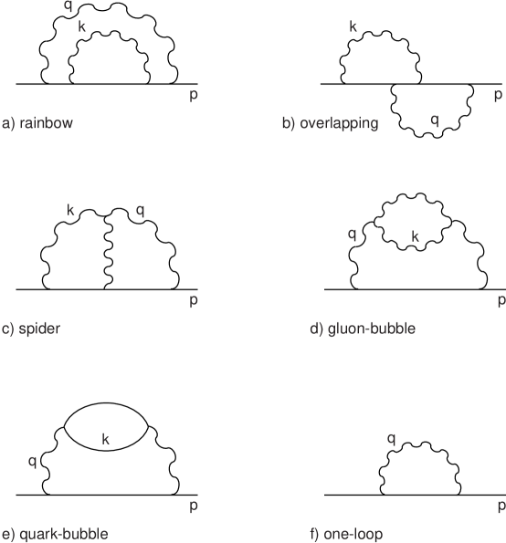
Figure 1: One- and two-loop quark self-energy diagrams for QCD. Wavy lines denote gluons, straight lines denote quarks. $p,q,$ and $k$ are four-momenta.

Whereas computation of Fig. 1f was straightforward, at least in hindsight, evaluation of the overlapping quark self-energy [4, 5] required the introduction of a new procedure, called the matrix integration technique. We recall that in this procedure, the two momentum integrals of $\int d^{2\omega}q\int d^{2\omega}kf(q,k)$, where $2\omega$ denotes the complex dimensionality of space-time, are integrated over $4\omega$-dimensional space in a single operation. We further recall that the biggest advantage of the matrix method is the ability to execute the momentum integrations exactly and in closed form. With the momentum integrals conveniently “out of the way”, we can then concentrate on the wide variety of new parameter singularities which is so characteristic of noncovariant-gauge multi-loop integrals. It turns out that the matrix method enables us to handle these new parameter singularities in a consistent and unambiguous manner. By comparison, multi-loop integrals with fewer and less severe parameter singularities may, in general, be evaluated by means of the nested method [4, 5, 6, 7]. In this traditional approach, the $2\omega$-momentum integrations are carried out sequentially.

We finally observe that the matrix integration technique works for covariant and noncovariant gauges alike, and regardless whether the integrals are massive or massless. We shall have occasion later in this article to highlight specific technical features of this powerful technique.

It is well known [8, 9] that in covariant gauges, QCD may be renormalized by a redefinition of the masses, coupling constants, and field normalizations. However, for noncovariant gauges, such as the light-cone gauge, the situation is more complicated: in addition to the same types of counterterms that arise in covariant gauges, for light-cone QCD we also require $n_{\mu}$-dependent counterterms. These noncovariant counterterms are different from any of the terms in the original Lagrangian density. On the other hand, and in contrast to the covariant case, no physical measurements are needed to fix the finite parts of these new noncovariant counterterms. Instead, the finite parts are constrained by the requirement that all physical observables be Lorentz-covariant. In a sense, the presumption of covariance of the observables constitutes an infinite set of physical constraints on the noncovariant counterterms.

In 1987, Bassetto, Dalbosco, and Soldati (BDS) [10, 11] proposed a renormalization scheme for light-cone QCD in which the particular types of noncovariant counterterms – permitted by gauge symmetry and Lorentz symmetry – are absorbed into the original Lagrangian density by means of noncovariant renormalizations of the quark and gluon fields. Unlike the covariant-gauge case, where the renormalization factors are scalars, in the BDS scheme the renormalization factors are matrices. The result is that the different spin-components of the quark and gluon fields are renormalized differently. The present two-loop calculations are a clear vindication of the BDS renormalization scheme.

The plan of paper (II) is as follows. In Section 2 we derive the integrands of the light-cone integrals for the various diagrams of Figure 1, and then break them down into approximately 80 simpler integrands. In Section 3 we illustrate, by means of examples, methods for handling the various integrations. The explicit values for the divergent parts of all integrals are tabulated in the Appendix. These results are analytic and allow for general quark masses. The counterterms needed for the renormalization of the quark self-energy to two loops in the light-cone gauge are derived in Section 4. It turns out that all required counterterms are local (that is, polynomial in the external momentum), and that their coefficients satisfy the relationships implied by the BDS renormalization scheme. The paper concludes in Section 5 with a summary of our results and their significance.

2 Derivation of the Integrals

The Lagrangian density for light-cone QCD reads

$${\cal L}\,=\ -{\textstyle\frac{1}{4}}F^{a}_{\mu\nu}F^{a\mu\nu}+\overline{\psi}_{\alpha}(i\partial\!\!\!/-m)\psi_{\alpha}+gT^{a}_{\alpha\beta}\overline{\psi}_{\alpha}A\!\!\!/^{a}\psi_{\beta}\,+{\cal L}_{\mathrm{f}ix}+{\cal L}_{\mathrm{g}h}+{\cal L}_{\mathrm{c}t}\,,\quad$$ (1)

where external source terms and quark flavor indices have been suppressed, and

$F^{a}_{\mu\nu}=\,\partial_{\mu}A^{a}_{\nu}-\partial_{\nu}A^{a}_{\mu}+gf^{abc}A^{b}_{\mu}A^{c}_{\nu}\,,\qquad\mu,\nu=0\,.\,.\,3,\qquad\partial_{\mu}\equiv\partial/\partial x^{\mu},$

$A^{a}_{\mu}(x)=\,$ gluon fields,$\qquad a,b,c=\,$ gluon indices$\,=1\,.\,.\,8\$ for SU(3),

$\psi_{\alpha}(x)=\,$ quark fields,$\qquad\alpha,\beta=\,$ color indices$\,=1,2,3,\qquad\overline{\psi}\equiv\psi^{\dagger}\gamma^{0},$

$A\!\!\!/\equiv\gamma\!\cdot\!A,\quad\partial\!\!\!/\equiv\gamma\!\cdot\!\partial,\quad$etc.$,\quad\gamma^{\mu}=\,$ Dirac matrices,$\quad(\gamma^{0})^{2}=1,$

$m=\,$ quark rest mass,$\quad g=\,$ coupling constant,

$T^{a}_{\alpha\beta}=\,$ generators of SU(3), normalized such that $[T^{a},T^{b}]=if^{abc}T^{c}$,

$f^{abc}=\,$ antisymmetric structure constants of SU(3) (with $f^{abc}f^{bcd}=3\delta^{ad}$),

${\cal L}_{\mathrm{f}ix}=\,$ gauge-fixing term $\,=\,-(n\!\cdot\!A)^{2}/(2\lambda),\$with $\lambda$ to be taken to zero later,

${\cal L}_{\mathrm{g}h}=\,$ ghost terms $\,=\,-\overline{\eta}^{a}(\delta^{ab}n\!\cdot\!\partial-gf^{abc}n\!\cdot\!A^{c})\eta^{b},\ \eta^{a}=\,$ ghost fields, and

${\cal L}_{\mathrm{c}t}=\,$ counterterms.

Repeated indices imply summation, and we use a $\,+,-,-,-\,$ metric for Minkowski space.

2.1 The Feynman Rules

The Lagrangian (1) leads to the following Feynman rules for light-cone QCD [11, 12, 13]:

Quark propagator:

$$i\delta_{\alpha\beta}S(p),\quad{\mathrm{w}ith}\qquad S(p)\equiv\frac{p_{\!}\!\!/+m}{p^{2}-m^{2}+i\theta}\,,\qquad\theta>0,$$ (2)

where $p_{\mu}$ is the quark 4-momentum, $\alpha$ and $\beta$ are color indices as in (1), and the $i\theta$ term is Feynman’s prescription for avoiding a singularity when $p^{2}=m^{2}$. (We let $\theta$ go to zero after Wick rotation.)

Gluon propagator: $\quad i\delta^{ab}G_{\mu\nu}(q),\ \$ with

$$G_{\mu\nu}(q)\equiv\frac{-1}{q^{2}+i\theta}\left(g_{\mu\nu}-\frac{n_{\mu}q_{\nu}+q_{\mu}n_{\nu}}{n\!\cdot\!q}+\frac{\lambda q^{2}q_{\mu}q_{\nu}}{(n\!\cdot\!q)^{2}}\right),\qquad\theta>0,$$ (3)

where $q_{\mu}$ is the gluon 4-momentum. The gauge-fixing parameter $\lambda$ is now taken to zero, causing the third term in parentheses to drop out.

Quark-quark-gluon vertex factor: $\quad ig\gamma^{\mu}T^{a}_{\alpha\beta}$.

3-gluon vertex factor: $\quad gf^{abc}\big{[}(p-q)^{\rho}g^{\mu\nu}+(q-k)^{\mu}g^{\nu\rho}+(k-p)^{\nu}g^{\mu\rho}\big{]},\quad$ where $p,q,k$ are the incoming 4-momenta of the attached gluons.

4-gluon vertex factor: $\ \ -ig^{2}\big{[}f^{abe}f^{cde}(g^{\mu\rho}g^{\nu\sigma}-g^{\mu\sigma}g^{\nu\rho})+f^{ace}f^{bde}(g^{\mu\nu}g^{\rho\sigma}-g^{\mu\sigma}g^{\nu\rho})+f^{ade}f^{cbe}(g^{\mu\rho}g^{\nu\sigma}-g^{\mu\nu}g^{\rho\sigma})\big{]}$.

Ghost propagator: $\quad\delta^{ab}/(n\!\cdot\!k),\quad$ where $k_{\mu}$ is the ghost 4-momentum.

Ghost-ghost-gluon vertex factor: $\ \ \,-igf^{abc}n^{\mu},\quad$ where $\mu$ and $a$ match indices of the attached gluon, while $b$ and $c$ match indices of the attached ghosts. Note that ghosts “decouple” in the light-cone gauge, because the ghost-ghost-gluon vertex factor is orthogonal to the gluon propagator (3) when $\lambda=0$ [14, 1].

Counterterm vertex factors:     to be determined in Section 4.

To construct the dimensionally regularized Green function for a diagram, we first impose conservation of momentum at each vertex, so that, apart from external momenta, there is only one independent momentum per loop. (In Figure 1, these momenta are denoted by $q$ and $k$.) We then form the product of the propagators and vertex factors for all internal lines and vertices, divide by $(2\pi)^{2\omega}$ for each loop, and integrate the resulting expression over the $2\omega$-dimensional space of each loop momentum. Finally, we multiply the integral by $-1$ for each internal quark loop, divide by $r!$ for each pair of vertices connected by $r$ gluon lines, and also divide by the number of permutations of the vertices which leave the diagram invariant (for fixed external lines) [11, 15]. In Figure 1, only diagram e (quark-bubble) has an internal quark loop, only diagram d (gluon-bubble) has a pair of vertices connected by more than one gluon line, and no diagram is invariant under a non-trivial permutation of its vertices.

The procedure just described gives only the “amputated” Green function, since it includes no factors for the external lines of the diagram.

2.2 The Integrals and the $n_{\mu}^{*}$-Prescription

To illustrate the application of the above Feynman rules, we may immediately write down the amputated Green function for the one-loop diagram of Figure 1f:

$$\delta_{\alpha\kappa}\Sigma_{1}(p)\ =\ \ \frac{-g^{2}T^{a}_{\alpha\beta}T^{a}_{\beta\kappa}}{(2\pi)^{2\omega}}\int_{M}\gamma^{\mu}S(p-q)\gamma^{\nu}\,G_{\mu\nu}(q)\,{\mathrm{d}}^{2\omega}q,\$$ (4)

where $\int_{M}$ denotes integration over Minkowski space, and $S$ and $G$ are the propagators defined in equations (2) and (3) (with $\lambda=0$, and $m$ equal to the rest mass of the external quark). To avoid a singularity in $G$ when $n\!\cdot\!q=0$ (in this and other integrals), we shall use the $n_{\mu}^{*}$-prescription (ML-prescription) [16, 2], in which

$$\frac{1}{n\!\cdot\!q}\ \to\ \lim_{\theta\to 0}\,\frac{n^{*}\!\!\cdot\!q}{n^{*}\!\!\cdot\!q\,n\!\cdot\!q+i\theta}\quad=\ \lim_{\theta\to 0}\,\frac{2n^{*}\!\!\cdot\!q}{n^{*}\!\!\cdot\!n\,q_{\|}^{2}+2i\theta}\,,\qquad\theta>0,$$ (5)

where $n_{\mu}^{*}$ is a new light-like 4-vector ($n^{*2}=0$), with $n^{*}\!\!\cdot\!n>0$ in Minkowski space, and

$$q_{\|\mu}\,\equiv\,\frac{n^{*}\!\!\cdot\!q\,n_{\mu}+n\!\cdot\!q\,n^{*}_{\mu}}{n^{*}\!\!\cdot\!n}\,,\qquad\quad q_{\perp\mu}\,\equiv\,q_{\mu}-q_{\|\mu}$$ (6)

for any 4-vector $q_{\mu}$. The same prescription applies to $(n\!\cdot\!k)^{-1}$, with the same $n^{*}_{\mu}$, but with $k$ in place of $q$. Prescription (5) was subsequently recovered in the context of canonical quantization by Bassetto et al. [17]. Unlike the old “principal value” prescription, the $n^{*}_{\mu}$-prescription is consistent with both Wick rotation and power-counting [1, 7, 11, 12].

The amputated Green functions for the five two-loop diagrams of Figure 1 possess the following structure:

Rainbow diagram: $\quad ig^{4}T^{a}_{\alpha\beta}T^{b}_{\beta\gamma}T^{b}_{\gamma\delta}T^{a}_{\delta\kappa}(2\pi)^{-4\omega}I_{\mathrm{a}},\ \$ with

$$I_{\mathrm{a}}\ \equiv\ \int_{M}\!{\mathrm{d}}^{2\omega}q\int_{M}\!{\mathrm{d}}^{2\omega}k\,\gamma^{\mu}S(p-q)\gamma^{\nu}S(p-q-k)\gamma^{\rho}S(p-q)\gamma^{\sigma}\,G_{\mu\sigma}(q)\,G_{\nu\rho}(k).$$

Overlapping diagram: $\quad ig^{4}T^{a}_{\alpha\beta}T^{b}_{\beta\gamma}T^{a}_{\gamma\delta}T^{b}_{\delta\kappa}(2\pi)^{-4\omega}I_{\mathrm{b}},\ \$ with

$$I_{\mathrm{b}}\ \equiv\ \int_{M}\!{\mathrm{d}}^{2\omega}q\int_{M}\!{\mathrm{d}}^{2\omega}k\,\gamma^{\mu}S(p-q)\gamma^{\nu}S(p-q-k)\gamma^{\rho}S(p-k)\gamma^{\sigma}\,G_{\mu\rho}(q)\,G_{\nu\sigma}(k).$$

Spider diagram: $\quad g^{4}f^{abc}T^{a}_{\alpha\beta}T^{b}_{\beta\gamma}T^{c}_{\gamma\kappa}(2\pi)^{-4\omega}I_{\mathrm{c}},\ \$ with

$$I_{\mathrm{c}}\! \equiv \!\int_{M}\!{\mathrm{d}}^{2\omega}q\int_{M}\!{\mathrm{d}}^{2\omega}k\,\gamma^{\sigma}S(p-q)\gamma^{\eta}S(p-k)\gamma^{\tau}\,G_{\mu\sigma}(q)\,G_{\nu\eta}(k-q)\,G_{\rho\tau}(k)\quad$$

$$\qquad\qquad\qquad\cdot\big{[}(k-2q)^{\rho}g^{\mu\nu}+(q-2k)^{\mu}g^{\nu\rho}+(q+k)^{\nu}g^{\mu\rho}\big{]}.$$

Gluon-bubble: $\quad\frac{1}{2}ig^{4}f^{abc}f^{bcd}T^{a}_{\alpha\beta}T^{d}_{\beta\kappa}(2\pi)^{-4\omega}I_{\mathrm{d}},\ \$ with

$$I_{\mathrm{d}}\! \equiv \!\int_{M}\!{\mathrm{d}}^{2\omega}q\int_{M}\!{\mathrm{d}}^{2\omega}k\,\gamma^{\phi}S(p-q)\gamma^{\xi}\,G_{\mu\phi}(q)\,G_{\nu\eta}(k-q)\,G_{\rho\tau}(k)\,G_{\sigma\xi}(q)$$

$$\qquad\qquad\quad\cdot\big{[}(k-2q)^{\rho}g^{\mu\nu}+(q-2k)^{\mu}g^{\nu\rho}+(q+k)^{\nu}g^{\mu\rho}\big{]}$$

$$\qquad\qquad\quad\cdot\big{[}(k-2q)^{\tau}g^{\sigma\eta}+(q-2k)^{\sigma}g^{\eta\tau}+(q+k)^{\eta}g^{\sigma\tau}\big{]}.$$

Quark-bubble: $\quad-ig^{4}T^{a}_{\alpha\beta}T^{a}_{\gamma\delta}T^{b}_{\delta\gamma}T^{b}_{\beta\kappa}(2\pi)^{-4\omega}I_{\mathrm{e}},\ \$ with $\ \ I_{\mathrm{e}}\ \equiv$

$$\int_{M}\!{\mathrm{d}}^{2\omega}q\int_{M}\!{\mathrm{d}}^{2\omega}k\,\gamma^{\mu}S(p-q)\gamma^{\nu}G_{\mu\sigma}(q)\frac{{\mathrm{T}race}[\gamma^{\sigma}(k\!\!\!/+m_{L})\gamma^{\rho}(k\!\!\!/-q\!\!\!/+m_{L})]}{[k^{2}-m_{L}^{2}+i\theta][(k-q)^{2}-m_{L}^{2}+i\theta]}G_{\rho\nu}(q),\ \$$ (7)

where $m_{L}$ is the rest mass of the quark in the inner loop of Figure 1e.

The first step in the evaluation of integrals $I_{\mathrm{a}}$ to $I_{\mathrm{d}}$ is to substitute for $S$ and $G$ from equations (2) and (3), and expand the numerator of each integrand into a sum of products. In order to avoid terms whose integrals diverge as $q\to 0$, the quark-bubble integral $I_{\mathrm{e}}$ will be handled differently from the other integrals, as discussed in Section 3.2.

Before integrating, we simplify the integrals by applying Wick rotations. This procedure is valid because both Feynman’s $i\theta$ prescription as well as the $n^{*}_{\mu}$-prescription lead to poles in the second and fourth quadrants only. In this way, the integral (4), for instance, becomes

$$\delta_{\alpha\kappa}\Sigma_{1}(p)\ =\,\ \frac{-ig^{2}T^{a}_{\alpha\beta}T^{a}_{\beta\kappa}}{(2\pi)^{2\omega}}\int_{E}\!{\mathrm{d}}^{2\omega}q\frac{\gamma^{\mu}(p_{\!}\!\!/-q\!\!\!/-m)\gamma^{\nu}}{[(p-q)^{2}+m^{2}]\,q^{2}}\left(\delta_{\mu\nu}-\frac{n_{\mu}q_{\nu}+q_{\mu}n_{\nu}}{n\!\cdot\!q}\right),$$

where $\,\mu,\nu=1\dots 4,\ q_{0}=iq_{4},\ p_{0}=ip_{4},\ n_{0}=in_{4},\ \gamma^{0}=i\gamma^{4},\,$ and $\int_{E}$ denotes integration over the Euclidean space spanned by $q_{1}\dots q_{4}$.

2.3 Expansion, Reduction, Transformation, and Tadpoles

From the Feynman rules, we see that Green functions in general are integrals of rational functions of the loop momenta. For integrals $I_{\mathrm{a}}$ to $I_{\mathrm{d}}$ above, it would appear that some terms in the numerators of the integrands could have degrees as high as 11 in $q$ and $k$ together (after up to four applications of the $n^{*}_{\mu}$-prescription (5)). Fortunately, however, we may reduce the maximum degree to five, and in most cases to three, by means of cancellations between terms within each integral, and between numerator and denominator factors within many of the terms. Because of the large number of terms involved, some computer assistance is advantageous.

Expanding the numerator of each integrand into a sum of products, and then following the procedure outlined in paper (I), we obtain a list of well over 100 distinct terms to be integrated. Fortunately, we can shorten this list still further by applying transformations, such as $k\to q-k,\ q\to q+k,$ and/or $q\leftrightarrow k$, to selected terms. The transformation $q\to q+k$, for instance, yields

$$\frac{n\!\!\!/}{(n\!\cdot\!q-n\!\cdot\!k)(q-k)^{2}[(p-q)^{2}+m^{2}]k^{2}}\ \to\ \frac{n\!\!\!/}{n\!\cdot\!q\,q^{2}[(p-q-k)^{2}+m^{2}]k^{2}}\,,$$

where the expression on the right just happens to be already on the list of terms to be integrated. Notice that the factor $(n\!\cdot\!q-n\!\cdot\!k)$ can thus be eliminated from all denominators.

Having carried out these various cancellations and transformations, we find that some of the integrands factor into separate $q$ and $k$ dependent parts. In some cases, one of these two one-loop integrals vanishes, since its integrand is antisymmetric under $q\to-q$ or $k\to-k$. In many other cases, one of the one-loop integrals corresponds to a massless tadpole, and likewise vanishes in the context of dimensional regularization [18, 19].

2.4 Power Counting

For renormalization, we require only the divergent parts of integrals $I_{\mathrm{a}}$ to $I_{\mathrm{e}}$, so we shall drop all terms whose integrals can be shown by power counting to converge when $\omega=2$. For a covariant gauge, Weinberg’s theorem [20, 15] tells us that a Feynman integral is UV-convergent if its integrand, including the measure $d^{4}q\,d^{4}k\dots$, is of negative degree with respect to every non-empty subset of the loop momenta $q,k,\dots$. We have the same rule for the light-cone gauge, except that we must also consider subsets that include only the “transverse” part – the part orthogonal to $n$ – of one or more of the loop momenta [11].

To illustrate power counting, consider the Euclidean-space integral

$$\int\int\frac{n\!\!\!/\,n\!\cdot\!p\,{\mathrm{d}}^{2\omega}q\,{\mathrm{d}}^{2\omega}k}{n\!\cdot\!q[(p-q)^{2}+m^{2}](q-k)^{2}(n\!\cdot\!q-n\!\cdot\!k)[(p-k)^{2}+m^{2}]}\,,$$ (8)

arising from the spider diagram (Figure 1c). When $\omega=2$, the integrand has degree $-2$ in $q$, $-1$ in $k$, and 0 in $q$ and $k$ combined. Hence, by the rule given above, this integral may be divergent. As it turns out, however, this particular integral is actually convergent, because the leading-order part of the integrand for large $|q|$ and $|k|$ is antisymmetric under $q_{3}\leftrightarrow q_{4},k_{3}\leftrightarrow k_{4}$ (we have taken $\,n_{1}=n_{2}=n^{*}_{1}=n^{*}_{2}=0\,$ for simplicity, so that $\,q_{\|\mu}=(0,0,q_{3},q_{4})\,$ and $\,k_{\|\mu}=(0,0,k_{3},k_{4})$). There are other such “borderline” integrals which are convergent for the same reason.

In the Appendix we have summarized the divergent terms which remain to be integrated, for each of the integrals $I_{a}$ to $I_{e}$. We have also listed there the various integrated divergent parts for each individual term. In the next section we shall demonstrate how these results were obtained.

3 Integration Methods

Several different approaches to the evaluation of multi-loop Feynman integrals appear in the literature [6, 7, 21, 22, 23]; they will not be reviewed here. In most methods, one begins by writing the denominator of the integrand as an integral, using a parametrization formula. We shall use the formula known as Schwinger’s representation:

$$\frac{1}{F_{1}^{\mathrm{u}}F_{2}^{\mathrm{v}}\dots}\ =\ \int_{0}^{\infty}\frac{\alpha_{1}^{\mathrm{u}-1}{\mathrm{d}}\alpha_{1}}{\Gamma(\mathrm{u})}\int_{0}^{\infty}\frac{\alpha_{2}^{\mathrm{v}-1}{\mathrm{d}}\alpha_{2}}{\Gamma(\mathrm{v})}\dots\ \,\exp{\Big{(}-\alpha_{1}F_{1}-\alpha_{2}F_{2}\dots\Big{)}}.\,\$$ (9)

The factors $F_{1},F_{2},\dots$ must have positive Real parts; hence, before using formula (9), we apply the $n^{*}_{\mu}$- prescription to any factors of $n\!\cdot\!q$ and $n\!\cdot\!k$ in the denominator, perform Wick rotations, set $\theta$ to zero, and take the factor(s) $n^{*}\!\!\cdot\!n$ from Eq. (5) outside of the integral. The component $p_{4}$ of the external momentum is regarded as Real until after integration has been completed.

3.1 The Nested Method

After parametrization, it is necessary to integrate over both the loop momenta and the parameters. The question of the most suitable order for these integrations naturally arises. To take advantage of known one-loop results, we might try the nested method, in which we integrate first over one of the loop momenta ($k$, say), then over the parameters associated with factors involving $k$, then over the other momentum $q$, and finally over the remaining parameters.

As an example, consider the divergent Euclidean-space integral

$$I_{1}\,=\,\int\int\frac{n\!\!\!/\,{\mathrm{d}}^{2\omega}q\,{\mathrm{d}}^{2\omega}k}{n\!\cdot\!q[(p-q)^{2}+m^{2}][(p-q-k)^{2}+m^{2}]k^{2}}\,,$$ (10)

arising from the overlapping and rainbow diagrams. Applying formula (9) to the $k$-dependent factors only, we obtain

$$I_{1}\,=\,\int\frac{n\!\!\!/\,{\mathrm{d}}^{2\omega}q}{n\!\cdot\!q\,Q}\int_{0}^{\infty}\!{\mathrm{d}}\alpha_{1}\int_{0}^{\infty}\!{\mathrm{d}}\alpha_{2}\int\!{\mathrm{d}}^{2\omega}k\,\exp{\Big{(}-\alpha_{1}[(p-q-k)^{2}+m^{2}]-\alpha_{2}k^{2}\Big{)}},$$

where $\,\ Q\equiv(p-q)^{2}+m^{2}.\ \,$ Next we change variables from $\ \alpha_{1},\alpha_{2}\$ to $\ A\equiv\alpha_{1}+\alpha_{2}\,$, $\,x\equiv\alpha_{1}/A,\,$ and complete the square in the exponent to get

$$I_{1}\,=\,\int\frac{n\!\!\!/\,{\mathrm{d}}^{2\omega}q}{n\!\cdot\!q\,Q}\int_{0}^{1}\!{\mathrm{d}}x\int_{0}^{\infty}\!A\,{\mathrm{d}}A\int\!{\mathrm{d}}^{2\omega}k\,\exp{\Big{(}-A[(k-xp+xq)^{2}+H]\Big{)}},$$ (11)

with $\,\ H\equiv x\Big{[}(1-x)(p-q)^{2}+m^{2}\Big{]}.\ \,$ The $k$ and $A$ integrations may then be carried out with the help of the well-known Gaussian and Gamma integrals:

$$\int\exp{(-Ar^{2})}\,{\mathrm{d}}^{2\omega}r=\left(\frac{\pi}{A}\right)^{\omega},\qquad\quad A>0,$$ (12)

and

$$\int_{0}^{\infty}A^{d}e^{-AH}\,{\mathrm{d}}A=\frac{\Gamma(d+1)}{H^{d+1}},\qquad\quad H>0,\ \ {\mathrm{R}e}\,d>-1,$$ (13)

respectively, with $\ r_{\mu}=k_{\mu}-x(p-q)_{\mu}\$ in this case. Accordingly, we obtain

$$I_{1}\ =\ \pi^{\omega}\Gamma({\textstyle\epsilon})\int\frac{n\!\!\!/\,{\mathrm{d}}^{2\omega}q}{n\!\cdot\!q\,Q}\int_{0}^{1}\!{\mathrm{d}}x\,H^{-{\textstyle\epsilon}};\quad\qquad{\textstyle\epsilon}\equiv 2-\omega.$$ (14)

From power counting, we expect the $k$ integral in Eq. (10) to be well defined only if $\omega<2$. In fact, we required just this condition in order to complete the integration (13) which produced the divergent factor $\Gamma({\textstyle\epsilon})$ in Eq. (14). The $q$ integral in Eq. (14) also diverges as ${\textstyle\epsilon}\to 0$, according to power counting, so altogether we expect $I_{1}$ to have a double pole at ${\textstyle\epsilon}=0$. This expectation will be confirmed by explicit calculation.

Before we can complete the integration, we must decide how to deal with the $q$-dependent factor $H^{-{\textstyle\epsilon}}$ in Eq. (14). Since we expect $I_{1}$ to have a double pole at ${\textstyle\epsilon}=0$, and since we are only interested in finding the divergent parts, we might try integrating only terms up to order $\,{\textstyle\epsilon}\,$ from the exponential series

$$H^{-{\textstyle\epsilon}}\!\! = \!\!1-{\textstyle\epsilon}\ln H+{\textstyle\frac{1}{2}}({\textstyle\epsilon}\ln H)^{2}-\dots~{},$$ (15)

$$= \!\!1-{\textstyle\epsilon}\ln x-{\textstyle\epsilon}\ln\Big{[}(1-x)(p-q)^{2}+m^{2}\Big{]}+{\textstyle\frac{1}{2}}({\textstyle\epsilon}\ln x)^{2}+\dots~{},$$ (16)

$$= \!\!x^{-{\textstyle\epsilon}}+\Big{[}(1-x)(p-q)^{2}+m^{2}\Big{]}^{-{\textstyle\epsilon}}-1+{\mathrm{O}}({\textstyle\epsilon}^{2}).$$ (17)

If we could drop the O$({\textstyle\epsilon}^{2})$ terms, we could immediately integrate over $x$, and then complete the $q$ integration from Eq. (14). Unfortunately, the series (15) cannot be integrated term-by-term, since it does not converge uniformly with respect to $q$, as explained in paper (I).

The convergence of series (15) is non-uniform partly because $H$ goes to infinity as $|q|$ goes to infinity. One way of solving this problem is to factor out the large $|q|$ behaviour before using a series, provided we do so without either creating new convergence problems, or generating terms that we cannot integrate. In the current example, we can extract a factor of $Q$ from $H$ before using the exponential series, so that Eqs. (15) to (17) become

$$H^{-{\textstyle\epsilon}}\!\! = \!\!Q^{-{\textstyle\epsilon}}\left(1-{\textstyle\epsilon}\ln\frac{H}{Q}+\frac{1}{2}\left[{\textstyle\epsilon}\ln\frac{H}{Q}\right]^{2}-\dots\right),$$

$$= \!\!Q^{-{\textstyle\epsilon}}\left(1-{\textstyle\epsilon}\ln x-{\textstyle\epsilon}\ln\left[\frac{(1-x)(p-q)^{2}+m^{2}}{Q}\right]+\frac{1}{2}({\textstyle\epsilon}\ln x)^{2}+\dots\right),$$

$$= \!\!Q^{-{\textstyle\epsilon}}\left(x^{-{\textstyle\epsilon}}+\left[\frac{(1-x)(p-q)^{2}+m^{2}}{Q}\right]^{-{\textstyle\epsilon}}-1+{\mathrm{O}}({\textstyle\epsilon}^{2})\right),$$ (19)

with $\,Q\equiv(p-q)^{2}+m^{2}$. Convergence of this new series remains uniform as $|q|\to\infty$, except near $x=0$ and $x=1$. Fortunately, however, these remaining non-uniformities cause no trouble, provided we integrate Eq. (19) only. At $x=0$, the $x^{-{\textstyle\epsilon}}$ term in this equation gives the correct contribution to the pole parts of $I_{1}$, while the contributions from the second and third terms in parentheses cancel. Similarly, as $x\to 1$, $|q|\to\infty$, the second term in parentheses gives the correct contribution, while the contributions from the first and third terms cancel. (One may check these claims by using expansions in powers of $x$ near $x=0$, and $1-x$ near $x=1$.) Hence, the O$({\textstyle\epsilon}^{2})$ term in Eq. (19) does not contribute to the pole parts of $I_{1}$.

Integrating Eq. (19) over $x$, and substituting into Eq. (14), we find that

$$I_{1}\ =\ \frac{\pi^{\omega}\Gamma({\textstyle\epsilon})}{1-{\textstyle\epsilon}}\int\frac{n\!\!\!/\,{\mathrm{d}}^{2\omega}q}{n\!\cdot\!q\,Q}\left[\frac{1+{\textstyle\epsilon}}{Q^{\textstyle\epsilon}}+\frac{m^{2}\big{[}Q^{-{\textstyle\epsilon}}-(m^{2})^{-{\textstyle\epsilon}}\big{]}}{(p-q)^{2}}\right]\quad+{\mathrm{\ }finite},\$$ (20)

where “finite” refers to terms which do not diverge as ${\textstyle\epsilon}\to 0$. By power counting, we see that the $q$ integration in Eq. (20) diverges only for the first term in square brackets. Because of the divergent factor $\Gamma({\textstyle\epsilon})$ in front, we need both the divergent and finite parts of the $q$ integral, but not parts of order ${\textstyle\epsilon}$. Hence, we may set ${\textstyle\epsilon}=0$ in the convergent second term, causing this term to vanish (fortuitously). Applying the $n^{*}_{\mu}$-prescription (5), along with the parametrization formula (9), we obtain

$$I_{1}\ =\ \frac{2n\!\!\!/\pi^{\omega}\Gamma({\textstyle\epsilon})(1+{\textstyle\epsilon})}{n^{*}\!\!\cdot\!n\,(1-{\textstyle\epsilon})}\int_{0}^{\infty}\!{\mathrm{d}}\alpha_{1}\int_{0}^{\infty}\frac{\alpha_{2}^{\textstyle\epsilon}\,{\mathrm{d}}\alpha_{2}}{\Gamma(1+{\textstyle\epsilon})}\int\!n^{*}\!\!\cdot\!q\,e^{-T}\,{\mathrm{d}}^{2\omega}q\ \ +{\mathrm{\ }finite},\qquad\qquad$$

$$=\ \frac{2n\!\!\!/\pi^{\omega}(1+{\textstyle\epsilon})}{n^{*}\!\!\cdot\!n\,{\textstyle\epsilon}(1-{\textstyle\epsilon})}\int_{0}^{1}\!y^{\textstyle\epsilon}{\mathrm{d}}y\int_{0}^{\infty}\!\!A^{1+{\textstyle\epsilon}}{\mathrm{d}}A\int\!n^{*}\!\!\cdot\!(r+yp_{\|}+p_{\perp})\,e^{-T}\,{\mathrm{d}}^{2\omega}r\ \ +{\mathrm{\ }finite},\ \$$ (21)

where $\quad A\equiv\alpha_{1}+\alpha_{2},\quad y\equiv\alpha_{2}/A,\quad r_{\mu}\equiv q_{\mu}-yp_{\|\mu}-p_{\perp\mu},\quad$ and

$$T\,\equiv\,\alpha_{1}q_{\|}^{2}+\alpha_{2}Q = A\Big{[}q_{\|}^{2}+yq_{\perp}^{2}-2yp\!\cdot\!q+y(p^{2}+m^{2})\Big{]},$$

$$= A\Big{[}r_{\|}^{2}+yr_{\perp}^{2}+y(1-y)p_{\|}^{2}+ym^{2}\Big{]}.$$

The 4-vectors $p_{\|\mu},\,p_{\perp\mu}$, and so on, are defined in Eqs. (6). Note that $\,n^{*}\!\!\cdot\!p_{\|}=n^{*}\!\!\cdot\!p$, $\,p\!\cdot\!q=p_{\|}\!\cdot\!q_{\|}+p_{\perp}\!\cdot\!q_{\perp},\ (p_{\|})_{\perp}=0,\,$ etc., for any 4-vectors $p_{\mu}$ and $q_{\mu}$.

Since $T$ is an even function of $r$, we may drop the term with $n^{*}\!\!\cdot\!r$ from the integrand of Eq. (21). We also drop $n^{*}\!\!\cdot\!p_{\perp}$, which is equal to zero, and factor the $r$ integral into independent $r_{\|}$ and $r_{\perp}$ parts:

$$\int y\,n^{*}\!\!\cdot\!p_{\|}\,e^{-T}\,{\mathrm{d}}^{2\omega}r = y\,n^{*}\!\!\cdot\!p\,\exp{\Big{(}-Ay\Big{[}(1-y)p_{\|}^{2}+m^{2}\Big{]}\Big{)}}$$

$$\times\ \int\exp{(-Ar_{\|}^{2})}\,{\mathrm{d}}^{2}r_{\|}\int\exp{(-Ayr_{\perp}^{2})}\,{\mathrm{d}}^{2\omega-2}r_{\perp}.$$

The integrations over $r,A$, and $y$ are then easily completed with the help of formulas (12) and (13).

3.2 The Quark-Bubble Integral $I_{\mathrm{e}}$

Let us try the nested method on the integral in Eq. (7). Since the inner loop of Figure 1e involves no gluons, the integral over $k$ of the $k$-dependent factors in (7) is just the standard covariant-gauge result [15]:

$$\int_{M}\!{\mathrm{d}}^{2\omega}k\,\frac{{\mathrm{T}race}[\gamma^{\sigma}(k\!\!\!/+m_{L})\gamma^{\rho}(k\!\!\!/-q\!\!\!/+m_{L})]}{[k^{2}-m_{L}^{2}+i\theta][(k-q)^{2}-m_{L}^{2}+i\theta]}\ =$$ (22)

$$\qquad\quad 8i\pi^{\omega}\Gamma({\textstyle\epsilon})(q^{2}g^{\sigma\rho}-q^{\sigma}q^{\rho})\int_{0}^{1}\!(x-x^{2})[m_{L}^{2}-(x-x^{2})q^{2}]^{-{\textstyle\epsilon}}{\mathrm{d}}x,\qquad$$

with $\theta>0$ and ${\textstyle\epsilon}\equiv 2-\omega$ as before. The above equation is exact: no terms of order $\,{\textstyle\epsilon}\,$, or higher, have been omitted. (To verify this claim, one may use the trace theorems [15] to obtain
Trace $\![\gamma^{\sigma}(k\!\!\!/+m_{L})\gamma^{\rho}(k\!\!\!/-q\!\!\!/+m_{L})]\ =\ 4g^{\sigma\rho}(m_{L}^{2}-k^{2}-q\!\cdot\!k)+8k^{\sigma}k^{\rho}-4q^{\sigma}k^{\rho}-4k^{\sigma}q^{\rho}$, and then carry out the $k$ integration using some of the formulas and methods from Subsection 3.1.)

Substituting the right-hand sides of Eqs. (22) and (2) into Eq. (7), we get

$$I_{\mathrm{e}}\,=\,8i\pi^{\omega}\Gamma({\textstyle\epsilon})\int_{M}\!{\mathrm{d}}^{2\omega}q\frac{\gamma^{\mu}(p_{\!}\!\!/-q\!\!\!/+m)\gamma^{\nu}}{(p-q)^{2}-m^{2}+i\theta}\,D_{\mu\nu}(q)\int_{0}^{1}\!\frac{(x-x^{2})\,{\mathrm{d}}x}{[m_{L}^{2}-(x-x^{2})q^{2}]^{\textstyle\epsilon}}\,,\ \$$ (23)

where $\ D_{\mu\nu}(q)\equiv G_{\mu\sigma}(q)(q^{2}g^{\sigma\rho}-q^{\sigma}q^{\rho})G_{\rho\nu}(q),\$ and $m$ is the rest mass of the external quark in Figure 1e. It follows from Eq. (3) that $\,D_{\mu\nu}(q)\to-G_{\mu\nu}(q)\,$ as $\,\theta,\lambda\to 0$, so that $I_{\mathrm{e}}$ is proportional to the one-loop integral (4), except for the extra $x$ integral within the $q$ integral. We note that there is only one factor of $q^{2}$ now in the denominator (in $D_{\mu\nu}(q)$), thereby preventing the integral from diverging as $q\to 0$.

After Wick rotation, Eq. (23) becomes

$$I_{\mathrm{e}}=\,8\pi^{\omega}\Gamma({\textstyle\epsilon})\int_{E}\!{\mathrm{d}}^{2\omega}q\,\frac{\gamma^{\mu}(p_{\!}\!\!/-q\!\!\!/-m)\gamma^{\nu}}{[(p-q)^{2}+m^{2}]\,q^{2}}\!\left(\delta_{\mu\nu}-\frac{n_{\mu}q_{\nu}+q_{\mu}n_{\nu}}{n\!\cdot\!q}\right)\!\int_{0}^{1}\frac{(x-x^{2})^{1-{\textstyle\epsilon}}\!\!}{L^{\textstyle\epsilon}}\,{\mathrm{d}}x,\ \$$ (24)

with $\,\ L\equiv q^{2}+m_{L}^{2}(x-x^{2})^{-1}.\ \,$ As in the example of Eq. (10), power counting tells us that integral (24) is well defined only if ${\textstyle\epsilon}>0$. Under this condition, $(q^{2})^{-{\textstyle\epsilon}}$ is a decreasing, concave-up function of $q^{2}$ (for $q^{2}>0$), from which it follows that

$$0\ <\ (q^{2})^{-{\textstyle\epsilon}}-L^{-{\textstyle\epsilon}}\ <\ (q^{2}-L)\frac{{\mathrm{d}}}{{\mathrm{d}}(q^{2})}\Big{[}(q^{2})^{-{\textstyle\epsilon}}\Big{]}\quad=\,\frac{{\textstyle\epsilon}\,m_{L}^{2}}{x-x^{2}}(q^{2})^{-{\textstyle\epsilon}-1}.\$$ (25)

Using this inequality, we can show by power counting that the difference between integral (24), and the same integral with $L$ replaced by $q^{2}$, remains finite as ${\textstyle\epsilon}\to 0$. Since we are merely interested in the divergent parts of $I_{\mathrm{e}}$, we may make this replacement and pull the factor $(q^{2})^{-{\textstyle\epsilon}}$ out of the $x$ integral. Integrating over $x$ with the help of the formula

$$\int_{0}^{1}x^{c}(1-x)^{d}{\mathrm{d}}x\ =\ \frac{\Gamma(c+1)\Gamma(d+1)}{\Gamma(c+d+2)}\,,\qquad{\mathrm{R}e}\,c,{\mathrm{R}e}\,d>-1,$$ (26)

and completing the $q$ integration, we get the desired result. Notice that the divergent parts of $I_{\mathrm{e}}$ will be independent of the mass of the quark in the inner loop, as $m_{L}$ enters Eq. (24) only by way of $L$.

3.3 Review of the Matrix Method

As seen in the preceding examples, in the nested method one tries to modify the integrand between the first and second momentum integrations, in a way that simplifies the final integration without changing the divergent parts of the result. Particular care must be taken with regard to the behaviour of the integrand near boundaries where the final integration diverges, such as $|q|\to\infty,\,x\to 0$ in the examples. The greater the degree of divergence, the more closely the “simplified” integrand must match the exact one. This requirement becomes more and more challenging as the number of $\alpha$ parameters increases.

For integrals such as

$$I_{2}\,=\,\int_{E}\int_{E}\,\frac{q\!\!\!/\ {\mathrm{d}}^{2\omega}q\,{\mathrm{d}}^{2\omega}k}{n\!\cdot\!q\,[(p-q)^{2}+m^{2}]\,[(p-q-k)^{2}+m^{2}]\,[(p-k)^{2}+m^{2}]\,k^{2}}\,,\$$ (27)

in which both $q$ and $k$ appear in more than two denominator factors each, it is easier to complete all momentum integrations before doing any parameter integrations. This approach is called the matrix method [4, 5]. Momentum integrations are straightforward with this method, because the combined $4\omega$-dimensional momentum integral can be expressed as a derivative of a product of one-dimensional Gaussian integrals. In view of the importance of the matrix method for multi-loop integrals, we shall briefly review its main features.

After Wick rotation and application of the $n^{*}_{\mu}$-prescription, a two-loop light-cone integral takes the form of an integral over $q$ and $k$ of a polynomial $P(q,k)$, say, divided by some non-negative quadratic factors $F_{1},F_{2},\dots$. Application of the parametrization formula (9) then yields

$$\int_{E}\!{\mathrm{d}}^{2\omega}q\int_{E}\!{\mathrm{d}}^{2\omega}k\,\frac{P(q,k)}{F_{1}F_{2}\dots}\ =\ \int_{0}^{\infty}\!{\mathrm{d}}\alpha_{1}\int_{0}^{\infty}\!{\mathrm{d}}\alpha_{2}\ \dots\ J[P(q,k)];\$$ (28)

$$J[P(q,k)]\ \equiv\ \int_{E}\!{\mathrm{d}}^{2\omega}q\int_{E}\!{\mathrm{d}}^{2\omega}k\,P(q,k)\,\exp{\Big{(}-\alpha_{1}F_{1}-\alpha_{2}F_{2}\dots\Big{)}}.\$$ (29)

Since the exponent is quadratic in $q$ and $k$, we can rewrite Eq. (29) in the form

$$J[P(q,k)]\ =\ \int_{E}\!{\mathrm{d}}^{4\omega}{\mathsf{z}}\,P(q,k)\,\exp{\mathsf{\Big{missing}}(-zMz^{\top}+2B\!\cdot\!z-C\Big{)}},\ \$$ (30)

where $\mathsf{M}$ is a Real $4\omega\!\times\!4\omega$ matrix, $\mathsf{B}$ and $\mathsf{z}$ are Real $4\omega$-vectors, ${\mathsf{z}}\equiv(k_{4},q_{4},\,k_{3},q_{3}$, $\dots),{\ }^{\top}$ denotes transpose, and the components of $\mathsf{M},\,B$, and $\mathsf{C}$ are functions of $\alpha_{1},\alpha_{2}\dots$, but not of $q$ or $k$.

For any given set of $F$ factors, one may obtain explicit expressions for the components of $\mathsf{M},\,B$, and $\mathsf{C}$ by expressing the exponents from Eqs. (29) and (30) in terms of the components of $q$ and $k$, and then equating corresponding coefficients. For the two-loop integrals of the Appendix, with $q_{\|}=(0,0,q_{3},q_{4})$ and $k_{\|}=(0,0,k_{3},k_{4})$ as before, we find that

$${\mathsf{M}}=A\left[\begin{array}[]{ccccccc}\!a&tG&&&&&\\ \!tG&\,1-a&&&&&\\ &&\!a&tG&&&\\ &&\!tG&\,1-a&&&\\ &&&&\!h&tG&\\ &&&&\!tG&\lambda&\\ &&&&&&\ddots\!\end{array}\right],\qquad{\mathsf{B}}^{\top}=A\left[\!\begin{array}[]{c}bp_{4}\\ \beta p_{4}\\ bp_{3}\\ \beta p_{3}\\ bp_{2}\\ \beta p_{2}\\ \vdots\end{array}\!\right],\quad$$ (31)

where the dots in $\mathsf{M}$ denote $2\omega-3$ repetitions of the third $2\!\times\!2$ sub-matrix, and $A(1-a),A\lambda,A\beta,AG,Ab,Ah$, and $Aa$ are the sums of the $\alpha$ parameters whose corresponding $F$ factors include $\quad q_{\|}^{2},\quad q_{\perp}^{2},\quad-2p\!\cdot\!q,\quad 2tq\!\cdot\!k,\quad-2p\!\cdot\!k,\quad k_{\perp}^{2},\quad k_{\|}^{2},\$ respectively. For example, if we label the denominator factors in integral (27) as $F_{1}$ to $F_{5}$ from left to right (after application of prescription (5), with $2n^{*}\!\!\cdot\!q/n^{*}\!\!\cdot\!n$ taken into $P$), we have for this integral

$$\qquad\ \left.\begin{array}[]{l}1-a=(\alpha_{1}+\alpha_{2}+\alpha_{3})/A,\qquad\lambda=\beta=(\alpha_{2}+\alpha_{3})/A,\qquad t=1,\\ h=a=(\alpha_{3}+\alpha_{4}+\alpha_{5})/A,\qquad b=(\alpha_{3}+\alpha_{4})/A,\qquad G=\alpha_{3}/A,\end{array}\ \ \ \right\}\!\!\!\!$$ (32)

$${\mathsf{C}}\ =\ (\alpha_{2}+\alpha_{3}+\alpha_{4})(p^{2}+m^{2})\ =\ A(b+\lambda-G)(p^{2}+m^{2}).\qquad$$ (33)

The equations for $\,a\,$ and $\,1-a\,$ tell us that $\,A=\alpha_{1}+\alpha_{2}+2\alpha_{3}+\alpha_{4}+\alpha_{5}$.

Since the matrix $\mathsf{M}$ is to be multiplied by $\mathsf{z}$ on both sides, it may always be constructed symmetrically. Accordingly, there exists a matrix $\mathsf{R}$ such that $\mathsf{R}MR^{\top}$ is diagonal and $\mathsf{R}^{\top}\!R=1$. Defining a new vector $\mathsf{y}$ so that $\mathsf{z}=yR+BM^{-1}$, and taking $P=1$, we find that Eq. (30) becomes

$$J[1]\ =\ \exp{\mathsf{\Big{missing}}(BM^{-1}B^{\top}-C\Big{)}}\int_{E}|\!\det\mathsf{R}|\,{\mathrm{d}}^{4\omega}y\,\exp{\Big{(}-yRMR^{\top}\!y^{\top}\Big{)}}.\ \$$ (34)

Since the integral in this equation is just a product of $4\omega$ one-dimensional Gaussian integrals, we may use formula (12), along with $\ \ |\!\det\mathsf{R}|=1\ \$ and $\ \ \prod_{i}({\mathsf{R}MR^{\top}})_{ii}=\det(\mathsf{R}MR^{\top})=\det M,\ \,$ to get

$$J[1]\ =\ \pi^{2\omega}(\det{\mathsf{M}})^{-1/2}\exp{\mathsf{\Big{missing}}(BM^{-1}B^{\top}-C\Big{)}}.$$ (35)

Notice that we never actually need to construct $\mathsf{R}$. To find $J[P]$ for general $P(q,k)$, we differentiate Eq. (30) partially with respect to ${\mathsf{B}}_{i}$ to obtain $\,\partial J[P]/\partial{\mathsf{B}}_{i}=2J[{\mathsf{z}}_{i}P]$, and then apply this formula repeatedly to Eq. (35) to get

$$\left.\begin{array}[]{rcl}J[{\mathsf{z}}_{i}]&=&{\mathsf{T}}_{i}J[1],\\ J[{\mathsf{z}}_{i}{\mathsf{z}}_{j}]&=&\Big{[}{\mathsf{T}}_{i}{\mathsf{T}}_{j}+({\textstyle\frac{1}{2}}{\mathsf{M}}^{-1})_{ij}\Big{]}J[1],\\ J[{\mathsf{z}}_{i}{\mathsf{z}}_{j}{\mathsf{z}}_{k}]&=&\Big{[}{\mathsf{T}}_{i}{\mathsf{T}}_{j}{\mathsf{T}}_{k}+{\mathsf{T}}_{i}({\textstyle\frac{1}{2}}{\mathsf{M}}^{-1})_{jk}+{\mathsf{T}}_{j}({\textstyle\frac{1}{2}}{\mathsf{M}}^{-1})_{ki}+{\mathsf{T}}_{k}({\textstyle\frac{1}{2}}{\mathsf{M}}^{-1})_{ij}\Big{]}J[1],\\ &\vdots&\end{array}\right\}$$ (36)

$${\mathrm{w}here}\quad{\mathsf{T}}\ \equiv\ {\mathsf{B}M}^{-1}\ \equiv\ (r_{4},s_{4},\ r_{3},s_{3},\,\dots\,).\qquad\qquad\qquad$$ (37)

Since the momentum integral $J[P]$ is a linear functional of $P$, and $\,{\mathsf{z}}\equiv(k_{4},q_{4},\,k_{3},q_{3}$, $\dots)$, we can use the above equations to find $J[P]$ for any polynomial $P(q,k)$.

In order to derive the two-loop integrals summarized in the Appendix, we substitute from Eqs. (31) into Eqs. (35) to (37) to obtain the following relations:

$$\quad J[k_{\mu}]\,=\,r_{\mu}J[1],\quad\qquad J[n^{*}\!\!\cdot\!q\,k_{\mu}]\,=\,\left(n^{*}\!\!\cdot\!s\,r_{\mu}-\frac{Gn^{*}_{\mu}}{2AD_{\|}}\right)J[1],\qquad$$

$$\quad J[q_{\mu}]\,=\,s_{\mu}J[1],\quad\qquad J[n^{*}\!\!\cdot\!q\,q_{\mu}]\,=\,\left(n^{*}\!\!\cdot\!s\,s_{\mu}+\frac{an^{*}_{\mu}}{2AD_{\|}}\right)J[1],\qquad$$ (38)

$$J[n^{*}\!\!\cdot\!q\,n\!\cdot\!k\,k_{\mu}]\ =\ \left(n^{*}\!\!\cdot\!s\,n\!\cdot\!r\,r_{\mu}+\frac{\beta n^{*}\!\!\cdot\!pn_{\mu}-Gn^{*}\!\!\cdot\!n(r+r_{\|})_{\mu}}{2AD_{\|}}\right)J[1],\qquad$$

$${\mathrm{a}nd\ so\ on,\ where}\qquad J[1]\,=\,\left(\frac{\pi}{A}\right)^{2\omega}\frac{e^{-AH}}{D_{\|}D_{\perp}^{\omega-1}}\,,\qquad\qquad\qquad\qquad\qquad\qquad$$ (39)

$$r_{\mu}\! = [(1-a)b-G\beta]\frac{p_{\|\mu}}{D_{\|}}+(\lambda b-G\beta)\frac{p_{\perp\mu}}{D_{\perp}}\,,$$ (40)

$$s_{\mu}\! = \qquad(a\beta-Gb)\frac{p_{\|\mu}}{D_{\|}}+(h\beta-Gb)\frac{p_{\perp\mu}}{D_{\perp}}\,,$$ (41)

$$H\! \equiv \frac{\mathsf{C}-BM^{-1}B^{\top}}{A}\ =\,\frac{\mathsf{C}}{A}-(br+\beta s)\!\cdot\!p,$$ (42)

$$D_{\|}\! \equiv a(1-a)-G^{2},\qquad\quad D_{\perp}\,\equiv\ \lambda h-G^{2}.$$ (43)

From the definitions of the new parameters following Eq. (31), one may show that the sub-determinants $D_{\|}$ and $D_{\perp}$ satisfy $D_{\|}\geq 0$, $D_{\perp}\geq 0$ for all allowed values of $a,\lambda,h$, and $G$, thereby justifying our use of formula (12) in the derivation of Eq. (35).

For the integral (27), the polynomial $P[q,k]$ is given by $P=2n^{*}\!\!\cdot\!qq\!\!\!//n^{*}\!\!\cdot\!n$. Since $h=a$ and $\beta=\lambda$ from Eqs. (32), it follows from Eqs. (38), (39), (41), (42), and (33) that

$$J[P]\! = \!\frac{2}{n^{*}\!\!\cdot\!n}\left[n^{*}\!\!\cdot\!p\frac{(a\lambda-Gb)^{2}}{D_{\|}}\left(\frac{p_{\!}\!\!/_{\|}}{D_{\|}}+\frac{p_{\!}\!\!/_{\!\perp}}{D_{\perp}}\right)+\frac{a\,n\!\!\!/^{*}}{2AD_{\|}}\right]\frac{\pi^{2\omega}e^{-AH}}{A^{2\omega}D_{\|}D_{\perp}^{\omega-1}}\,;\$$ (44)

$$H\! = \!(b+\lambda-G)(p^{2}+m^{2})-(br+\lambda s)\!\cdot\!p.$$ (45)

3.4 Parameter Integration for the Matrix Method

Once $J[P]$ is known for a particular integral, we must complete the parameter integrations in Eq. (28). For the two-loop integrals listed in the Appendix, we begin these integrations by changing variables from $\alpha_{1},\alpha_{2},\dots$ to the applicable subset of the new parameters $\lambda,\beta,G,b,h,a$ and $A$, defined after Eq. (31). For the sample integral (27), we find from Eqs. (32) that

$$\int_{0}^{\infty}\!{\mathrm{d}}\alpha_{1}\int_{0}^{\infty}\!{\mathrm{d}}\alpha_{2}\,\dots\,J\ \,=\ \int_{0}^{1/2}\!{\mathrm{d}}G\int_{G}^{1-G}\!{\mathrm{d}}a\int_{G}^{1-a}\!{\mathrm{d}}\lambda\int_{G}^{a}\!{\mathrm{d}}b\int_{0}^{\infty}\!JA^{4}{\mathrm{d}}A.\$$ (46)

The integration ranges of the “finite” parameters $\lambda,\beta,G,b,h$, and $a$ depend on which $F$ factors are present in the original integral. For instance, if the factor containing $q+k$ in Eq. (27) did not also contain $p$, the $b$ integration in Eq. (46) would run from $0$ to $a-G$, rather than from $G$ to $a$. In the event of a repeated $F$ factor, there will be an additional finite parameter which can be integrated out immediately, since $J$ will not depend on it.

We see from Eqs. (43) and (45) that $D_{\|},\,D_{\perp}$, and $H$ are independent of $A$, so that the $A$ integration in Eq. (46) is straightforward. Applying formula (13) to Eq. (44), we obtain

$$\int_{0}^{\infty}\!J[P]A^{4}{\mathrm{d}}A\ =\ \frac{\pi^{2\omega}}{n^{*}\!\!\cdot\!n}\Big{[}\Gamma(1+2{\textstyle\epsilon})J_{1}+\Gamma(2{\textstyle\epsilon})J_{0}\Big{]};\ \quad{\textstyle\epsilon}\equiv 2-\omega,$$ (47)

where

$$J_{1}\,=\,\frac{2n^{*}\!\!\cdot\!p\,(a\lambda-Gb)^{2}}{D_{\|}^{2}D_{\perp}^{1-{\textstyle\epsilon}}H^{1+2{\textstyle\epsilon}}}\left(\frac{p_{\!}\!\!/_{\|}}{D_{\|}}+\frac{p_{\!}\!\!/_{\!\perp}}{D_{\perp}}\right),\qquad J_{0}\,=\,\frac{n\!\!\!/^{*}aH^{-2{\textstyle\epsilon}}}{D_{\|}^{2}D_{\perp}^{1-{\textstyle\epsilon}}}\,.\$$ (48)

Note that the use of formula (13) requires $H>0$. We can see that this requirement is satisfied in general by examining the way in which $H$ was constructed: since the $F$ factors and $\alpha$ parameters in Eq. (28) are non-negative, we find that the exponents in (29) and (30) are $\leq 0$ for all values of $q$ and $k$. Consequently, the sum of the exponents in Eq. (34) is $\leq 0$ for all values of $\mathsf{y}$. Taking $\mathsf{y}=0$, and noting that $A$ is just a sum of $\alpha$ parameters, we see that $H$ in Eq. (42) is $\geq 0$ for all allowed values of the old or new parameters. Furthermore, since $r_{\mu}$ and $s_{\mu}$ are independent of the quark mass $m$, one can deduce from Eq. (45) that $H=0$ only if $\,b+\lambda-G=0$ ($m\neq 0$). We emphasize that the relationship $\,b+\lambda-G=0\,$ applies specifically to the integral (27).

The presence of the divergent factor $\Gamma(2{\textstyle\epsilon})$ in Eq. (47) reflects the UV-divergence of integral (27) with respect to $q$ and $k$ combined. Additional divergences, known as subdivergences, may be found when we complete the remaining integrations from Eq. (46), because $J_{0}$ and $J_{1}$ go to infinity at the boundaries of the integration region where $a\to 0$ and $a\to 1$ (corresponding to $|k|\to\infty$ and $|q|\to\infty$, respectively). In the current example, each of these boundaries has three fewer dimensions than the full finite-parameter space, because from the limits of integration in (46) it follows that

$$a\ \geq\ b\ \geq\ G\ \geq\ 0\qquad{\mathrm{a}nd}\qquad 1-a\ \geq\ \lambda\ \geq\ G\ \geq\ 0.$$ (49)

Thus, near $a=1$, for instance, we could transform $dGd\lambda$ to $(1-a)^{2}dxdy$ (with $x$ and $y$ being finite parameters such that $\lambda=x(1-a)$ and $G=y(1-a)$). A subdivergence can therefore occur at $a=1$ only if the integrand $J_{0}$ or $J_{1}$ diverges there at least as fast as $(1-a)^{-3}$.

From Eqs. (43), (48), and (49), we find that $D_{\|},D_{\perp}\to 0$ linearly as $a\to 1$, while the numerator of $J_{1}$ goes to zero quadratically, and $H$ remains positive unless $b\to 0$ as well (assuming $m\neq 0$, as discussed above). Thus, we find that $J_{0}$ is of order $(1-a)^{{\textstyle\epsilon}-3}$ near $a=1$, $b\neq 0$, while $J_{1}$ is of order $(1-a)^{{\textstyle\epsilon}-2}$ there. Hence, by the criterion given above, the integral of $J_{0}$ over the finite parameters diverges as $a\to 1$ (and ${\textstyle\epsilon}\to 0$), while the integral of $J_{1}$ does not. Similar analyses at other boundaries of the integration region (including the case $a=1$, $b=0$) show that there are no other subdivergences in this example. Since we are only interested in finding the divergent parts of $I_{2}$, and since $J_{1}$ gives no subdivergences and is not multiplied by a divergent Gamma function in Eq. (47), we may drop $J_{1}$.

Due to the factor $\Gamma(2{\textstyle\epsilon})$ in Eq. (47), the subdivergence in the integral of $J_{0}$ will contribute a double pole to $I_{2}$, while the finite part of the same integral will contribute to the single pole. The factor $H^{-2{\textstyle\epsilon}}$ in Eq. (48) complicates the integration of $J_{0}$, but some simplification is possible because this factor affects the pole parts of $I_{2}$ only by way of the subdivergence at $a=1$. To begin the simplification, we rewrite $H^{-2{\textstyle\epsilon}}$ in (48) as $1+(H^{-2{\textstyle\epsilon}}-1)$, and then expand the factors, multiplying the term $(H^{-2{\textstyle\epsilon}}-1)$, in powers of $1-a$, $\lambda$, and $G$, using the definitions for $D_{\|}$ and $D_{\perp}$ from Eq. (43). In this fashion we obtain

$$J_{0}\ =\ \frac{n\!\!\!/^{*}a}{D_{\|}^{2}D_{\perp}^{1-{\textstyle\epsilon}}}+\frac{n\!\!\!/^{*}(H^{-2{\textstyle\epsilon}}-1)}{(1-a)^{2}\lambda^{1-{\textstyle\epsilon}}}\Big{[}1+{\mathrm{O}}(1-a,\lambda,G)\Big{]}.$$ (50)

By counting powers of $1-a,\lambda$, and $G$, we see that the integral of the term involving $(H^{-2{\textstyle\epsilon}}-1)$O$(1-a,\lambda,G)$ has no subdivergence; to find its finite part we therefore can set ${\textstyle\epsilon}=0$ in this term (which happens to make it vanish). Accordingly, we may replace $J_{0}$ by $\widehat{J}_{0}(H)$,

$$\widehat{J}_{0}(H)\ \equiv\ \frac{n\!\!\!/^{*}a}{D_{\|}^{2}D_{\perp}^{1-{\textstyle\epsilon}}}+\frac{n\!\!\!/^{*}(H^{-2{\textstyle\epsilon}}-1)}{(1-a)^{2}\lambda^{1-{\textstyle\epsilon}}}\,,$$ (51)

without affecting the divergent parts of $I_{2}$.

The next step is to replace $H$ in Eq. (51) by

$$H_{1}\ \equiv\ \lim_{a\to 1}H\ =\ b(p^{2}+m^{2})-b^{2}p^{2},$$

where the result on the right follows from Eqs. (45), (40), (43), (49), and from the equality $\beta=\lambda$ in Eqs. (32). To justify this replacement, we use the same kind of reasoning that led to the inequality (25); in the present case, an appropriate inequality is given by

$$0\ \ \leq\ \ |H^{-2{\textstyle\epsilon}}-H_{1}^{-2{\textstyle\epsilon}}|\ \ \leq\ \ 2{\textstyle\epsilon}|H-H_{1}|\,(H^{-2{\textstyle\epsilon}-1}+H_{1}^{-2{\textstyle\epsilon}-1}),$$

which holds for all allowed values of the parameters. Exploiting this new inequality, and noting that $|H-H_{1}|$ goes to zero as $a\to 1$, and that both $H$ and $H_{1}$ go to zero (linearly) only when $b\to 0$, we can show that the integral of $\,\widehat{J}_{0}(H)-\widehat{J}_{0}(H_{1})\,$, over the finite parameters, has no subdivergence and vanishes when ${\textstyle\epsilon}\to 0$. In summary, we can replace $H$ by $H_{1}$ in Eq. (51) without affecting the divergent parts of $I_{2}$.

Making this replacement, and integrating over $b$ in accordance with Eq. (46), we obtain

$$\int_{G}^{a}\widehat{J}_{0}(H_{1}){\mathrm{d}}b\ =\ \frac{n\!\!\!/^{*}a(a-G)}{D_{\|}^{2}D_{\perp}^{1-{\textstyle\epsilon}}}+\frac{n\!\!\!/^{*}\lambda^{{\textstyle\epsilon}-1}}{(1-a)^{2}}\!\left[\int_{0}^{1}\!-\!\int_{0}^{G}\!-\!\int_{a}^{1}\right]\!(H_{1}^{-2{\textstyle\epsilon}}-1){\mathrm{d}}b.\$$ (52)

As $a\to 1$, the ranges of the second and third integrals in square brackets shrink to points, so that these terms contribute no subdivergences to the total integral over the remaining parameters. Hence, in the derivation of the finite parts of the integrals of these terms, we are allowed to set ${\textstyle\epsilon}=0$ in their integrand (causing it to vanish). To facilitate the remaining $b$ integration in Eq. (52), we shall express $H_{1}^{-2{\textstyle\epsilon}}$ in the form (cf. Eq. (17)),

$$H_{1}^{-2{\textstyle\epsilon}}\ =\ [b(p^{2}+m^{2})-b^{2}p^{2}]^{-2{\textstyle\epsilon}}\ =\ (p^{2}+m^{2}-bp^{2})^{-2{\textstyle\epsilon}}+b^{-2{\textstyle\epsilon}}-1+{\mathrm{O}}({\textstyle\epsilon}^{2}).$$

It now remains to integrate the factor multiplying the $b$ integral in Eq. (52) over $\lambda,a$, and $G$, in accordance with Eq. (46). But this task is easy: since the $b$ integral is of order ${\textstyle\epsilon}$, only the divergent part of the integral over $\lambda,a$, and $G$ is needed.

Finally, we must also integrate the first term on the right-hand side of Eq. (52) over $\lambda,a$, and $G$, again in accordance with Eq. (46). Because of the factor $\Gamma(2{\textstyle\epsilon})$ in Eq. (47), both the divergent and finite parts of this triple integral will be needed. We begin the integration process by defining the new variables $\ x=D_{\perp}/a^{2},\ y=D_{\|}/a^{2},\$ and $\ v=G/a,\,$ so that

$$\int_{0}^{1/2}\!{\mathrm{d}}G\int_{G}^{1-G}\!{\mathrm{d}}a\int_{G}^{1-a}\!{\mathrm{d}}\lambda\frac{a(a-G)}{D_{\|}^{2}D_{\perp}^{1-{\textstyle\epsilon}}}\ =\ \int_{0}^{1}\!{\mathrm{d}}v\int_{v-v^{2}}^{\infty}\!{\mathrm{d}}y\int_{v-v^{2}}^{y}\frac{a^{2{\textstyle\epsilon}}(1-v)}{y^{2}\,x^{1-{\textstyle\epsilon}}}{\mathrm{d}}x.$$

From the definitions of $y,\,v$, and $D_{\|}$, we find that $\,a^{2{\textstyle\epsilon}}=(y+v^{2}+1)^{-2{\textstyle\epsilon}}$. But this factor can be simplified because it affects the divergent and finite parts of the integral only at subdivergences. The subdivergence at $a=1$ now manifests itself at $\,v=y=x=0$. Near this point, we have

$$(y+v^{2}+1)^{-2{\textstyle\epsilon}}\ =\ 1-2{\textstyle\epsilon}(y+v^{2})+{\textstyle\epsilon}(1+2{\textstyle\epsilon})(y+v^{2})^{2}-\dots\,.$$ (53)

Only the first term of this series gives a subdivergence, so we may set ${\textstyle\epsilon}=0$ in the other terms (causing them to vanish, as usual). Away from the subdivergence, the integral is finite, so we can take ${\textstyle\epsilon}=0$ in that region as well. Thus, in the current example, the factor $a^{2{\textstyle\epsilon}}$ may be replaced by 1. The integrations over $x,\,y$, and $v$ pose no further problems.

For a subdivergence at $a=0$, we would use

$$(y+v^{2}+1)^{-2{\textstyle\epsilon}}\ =\ y^{-2{\textstyle\epsilon}}\Big{[}1-2{\textstyle\epsilon}(v^{2}+1)/y+{\textstyle\epsilon}(1+2{\textstyle\epsilon})(v^{2}+1)^{2}/y^{2}-\dots\Big{]},$$

valid for large $y$. If the subdivergence comes only from the first term in this series, then $a^{2{\textstyle\epsilon}}$ may be replaced by $y^{-2{\textstyle\epsilon}}$.

3.5 Reduction of Subdivergences

The subdivergence in integral (27) is of the mildest possible nature; that is, $J_{0}$ goes to infinity only just fast enough to make the finite-parameter integral diverge as $a\to 1$ and ${\textstyle\epsilon}\to 0$. For this reason, we were able to drop the O$(1-a)$ term in Eq. (50), replace $H$ by $H_{1}$, drop the last two integrals in Eq. (52), and drop all but the first term of series (53). For an integral with a more severe subdivergence, it may be helpful to begin with a partial calculation by the nested method, thereby reducing the degree of divergence with respect to one of the loop momenta before applying the full matrix method.

A good example is the Euclidean-space integral

$$I_{3}\,=\,\int\int\frac{P_{\mu\nu}(q,n,p)\ k^{\mu}k^{\nu}\,\ {\mathrm{d}}^{2\omega}q\,{\mathrm{d}}^{2\omega}k}{[(q-k)^{2}+m^{2}]\,[k^{2}+m^{2}]\,F_{3}(q)F_{4}(q)\dots}\,,$$ (54)

in which $P_{\mu\nu}$ and $F_{3},F_{4},\dots$ do not depend on $k$. Because of the quadratic subdivergence as $|k|\to\infty$, a direct application of the matrix method would lead to a finite-parameter integral proportional to $\int a^{{\textstyle\epsilon}-2}{\mathrm{d}}a$ near $a=0$ (after all parameters except $a$ had been integrated out). To avoid having to deal with such a severe subdivergence, we proceed in the spirit of Eq. (11) by parametrizing the $k$-dependent denominator factors only, to get

$$I_{3}\,=\,\int\frac{P_{\mu\nu}{\mathrm{d}}^{2\omega}q}{F_{3}F_{4}\dots}\int_{0}^{1}\!{\mathrm{d}}v\int_{0}^{\infty}\!AY[k^{\mu}k^{\nu}]{\mathrm{d}}A,$$ (55)

where

$$Y[f(k)]\,\equiv\,\int\!{\mathrm{d}}^{2\omega}k\,f(k)\exp\Big{(}-A[k^{2}-2vq\!\cdot\!k+vq^{2}+m^{2}]\Big{)}.$$ (56)

Since Eq. (56) has the same form as Eq. (30) (with $\ {\mathsf{z}}=k,\ {\mathsf{M}}=A,\ {\mathsf{B}}=Avq,\$ and $\ {\mathsf{C}}=A(vq^{2}+m^{2})$), application of Eqs. (35) and (36) yields

$$Y[1]\,=\,\left(\frac{\pi}{A}\right)^{\omega}e^{-AL},\qquad Y[k^{\mu}k^{\nu}]\,=\,\Big{[}v^{2}q^{\mu}q^{\nu}+{\textstyle\frac{1}{2}}\delta^{\mu\nu}A^{-1}\Big{]}\left(\frac{\pi}{A}\right)^{\omega}e^{-AL},$$

with $\,\ L\equiv(v-v^{2})q^{2}+m^{2}.\ \,$ We next use formula (13) and Eq. (56) to obtain

$$\int_{0}^{\infty}\!AY[k^{\mu}k^{\nu}]{\mathrm{d}}A\ =\ \frac{\pi^{\omega}\Gamma({\textstyle\epsilon})E^{\mu\nu}}{L^{\textstyle\epsilon}}\,=\,E^{\mu\nu}\int_{0}^{\infty}\!AY[1]{\mathrm{d}}A\\ \,=\,\int_{0}^{\infty}\!AY[E^{\mu\nu}]{\mathrm{d}}A,\$$ (57)

where $\ E^{\mu\nu}\equiv v^{2}q^{\mu}q^{\nu}+L\delta^{\mu\nu}/(2{\textstyle\epsilon}-2).\ \,$

From the left and right ends of Eq. (57), we see that $I_{3}$ is unchanged if we replace the $k$-dependent argument $k^{\mu}k^{\nu}$ in Eq. (55) by the parameter-dependent polynomial $E^{\mu\nu}(q,v)$, thereby reducing the degree of the subdivergence. We then cancel $F$ factors, wherever possible, with factors in the terms of $P_{\mu\nu}E^{\mu\nu}$, parametrize the remaining $F$ factors in accordance with formula (9), and finally complete the integration by using either the matrix method or the nested method, whichever is easier to apply.

4 Renormalization

Wherever a quark line appears in a physical process, any one of the diagrams of Figure 1, as well as higher-loop diagrams, could also appear. Hence, the effective quark propagator $\,i\delta_{\alpha\beta}S_{\mathrm{e}ff}$ is the sum of the bare propagator $\,i\delta_{\alpha\beta}S\,$ from Subsection 2.1, plus contributions from self-energy processes with one loop, two loops, and so on:

$$iS_{\mathrm{e}ff}\! = \!iS+iS\Sigma_{1}iS+iS\Big{(}\Sigma_{1}iS\Sigma_{1}+\Sigma_{2}\Big{)}iS+\dots,$$ (58)

$$= \!iS+iS\Big{(}\Sigma_{1}+\Sigma_{2}+\dots\Big{)}iS_{\mathrm{e}ff},$$ (59)

where $\Sigma_{1}$ is the one-loop amputated Green function defined by Eq. (4), $\Sigma_{2}$ is the sum of the Green functions for the two-loop diagrams of Figures 1a to 1e, and so on. ($\Sigma_{2}$ will also include amplitudes of one-loop processes with counterterm vertices, as explained below.) Since $\Sigma_{j}$ is proportional to $g^{2j}$, $j=1,2,3,\dots$, the right-hand side of (58) is a power series in $g^{2}$. Similar series may be constructed for the effective gluon propagator and vertex factors:

$$i\delta^{ab}(G_{\mathrm{e}ff})_{\mu\nu}\! = \!i\delta^{ab}G_{\mu\nu}+iG_{\mu\sigma}\Big{[}\Pi_{(1)}^{ab\sigma\rho}+\Pi_{(2)}^{ab\sigma\rho}\Big{]}iG_{\rho\nu}+\dots,$$ (60)

$$(\Gamma_{\mathrm{e}ff})^{a\mu}_{\alpha\beta}\! = \!ig\gamma^{\mu}T^{a}_{\alpha\beta}+\Big{[}\Gamma^{a\mu}_{(1)\alpha\beta}+\Gamma^{a\mu}_{(2)\alpha\beta}\Big{]}+\dots,$$ (61)

etc., where $\Pi_{(1)}$, $\Pi_{(2)}$, $\Gamma_{(1)}$, and $\Gamma_{(2)}$ are the amputated Green functions of the one-loop processes shown in Figures 2b to 2e. For the light-cone gauge, we have, in Minkowski space [3, 11, 15],

$$\Sigma_{1}(p)\! = \!-i\widetilde{\alpha}_{s}C_{F}\left(2m-p_{\!}\!\!/+\frac{n\!\!\!/n\!\!\!/^{*}p_{\!}\!\!/+p_{\!}\!\!/n\!\!\!/^{*}n\!\!\!/}{n^{*}\!\!\cdot\!n}\right)\ \ +{\mathrm{f}inite},$$ (62)

$$\Gamma^{a\mu}_{(1)\alpha\beta}\! = \!i\widetilde{\alpha}_{s}gT^{a}_{\alpha\beta}\left(\frac{N_{C}}{2}-C_{F}\right)\left(\gamma^{\mu}+2\frac{n\!\!\!/\,n^{*\mu}-n\!\!\!/^{*}\,n^{\mu}}{n^{*}\!\!\cdot\!n}\right)\ +{\mathrm{f}inite},$$ (63)

$$\Gamma^{a\mu}_{(2)\alpha\beta}(k)\! = \!-i\widetilde{\alpha}_{s}gT^{a}_{\alpha\beta}\frac{N_{C}}{2}\left(\gamma^{\mu}-2\frac{n\!\!\!/\,n^{*\mu}+n\!\!\!/^{*}n^{\mu}}{n^{*}\!\!\cdot\!n}+4\frac{n^{*}\!\!\cdot\!k\,n\!\!\!/\,n^{\mu}}{n\!\cdot\!k\,n^{*}\!\!\cdot\!n}\right)\ +{\mathrm{f}inite},$$ (64)

$$\Pi_{(2)}^{ab\mu\nu}(q)\! = \!i\widetilde{\alpha}_{s}\delta^{ab}N_{C}\left[\frac{11}{3}\Big{(}q^{2}g^{\mu\nu}-q^{\mu}q^{\nu}\Big{)}+\frac{2n\!\cdot\!q}{n^{*}\!\!\cdot\!n}\left(\left[q^{\mu}-\frac{q^{2}n^{\mu}}{n\!\cdot\!q}\right]\left[n^{*\nu}-\frac{n^{*}\!\!\cdot\!q\,n^{\nu}}{n\!\cdot\!q}\right]\right.\right.$$ (65)

$$\qquad\qquad\qquad+\,\left.\left.\left[q^{\nu}-\frac{q^{2}n^{\nu}}{n\!\cdot\!q}\right]\left[n^{*\mu}-\frac{n^{*}\!\!\cdot\!q\,n^{\mu}}{n\!\cdot\!q}\right]\right)\right]\ +{\mathrm{f}inite},$$

$$\Pi_{(1)}^{ab\mu\nu}(q)\! = \!-i\widetilde{\alpha}_{s}\delta^{ab}\frac{2}{3}N_{f}\Big{(}q^{2}g^{\mu\nu}-q^{\mu}q^{\nu}\Big{)}\ +{\mathrm{f}inite};$$ (66)

here, $p,\,q$, and $k$ are external momenta as shown in Figure 2, $C_{F}=$ “color factor” $=\frac{4}{3}\ \,(\delta_{\alpha\kappa}C_{F}\equiv T^{a}_{\alpha\beta}T^{a}_{\beta\kappa}),\ N_{f}=$ number of quark flavors $=6,\ N_{C}=$ number of colors $=3\ \,(\delta^{ad}N_{C}\equiv f^{abc}f^{bcd}),\,$ and

$$\widetilde{\alpha}_{s}\equiv g^{2}\Gamma(2-\omega)(4\pi)^{-\omega}$$

in the “modified minimal subtraction” scheme, $\overline{\mathrm{M}S}$.

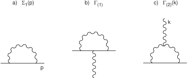
Figure 2: One-loop subgraphs of Figures 1a to 1e, with their amplitudes. Wavy lines denote gluons, straight lines quarks. $p,\,q$, and $k$ are four-momenta.

Most of the terms in Eqs. (58), (60), and (61) diverge as $\omega\to 2$. To make the effective propagators and vertex factors finite, we modify the Lagrangian density (1) in such a way that the bare propagators and vertex factors $S$, $G$, $ig\gamma^{\mu}$, etc. will be replaced by renormalized propagators and vertex factors. For instance, if we let

$$m\,\ \to\,\ m-\delta m\quad\qquad{\mathrm{a}nd}\quad\qquad\psi\ \,\to\,\ \psi+N\psi$$ (67)

in Eq. (1), where $N$ and $\delta m$ are both of order $g^{2}$, then the quark propagator in Eq. (2) becomes

$$S_{\mathrm{r}en}(p)\,=\,\Big{[}(1+\gamma^{0}N^{\dagger}\gamma^{0})(p_{\!}\!\!/-m+\delta m)(1+N)\Big{]}^{-1},$$ (68)

$$=\,S(p)-S(p)\Big{[}\delta m+\gamma^{0}N^{\dagger}\gamma^{0}(p_{\!}\!\!/-m)+(p_{\!}\!\!/-m)N\Big{]}S(p)\ +{\mathrm{O}}(g^{4}),\$$ (69)

where the $i\theta$ term has been suppressed for clarity. At the same time, we see from Eq. (58) that in order to make $S_{\mathrm{e}ff}$ finite, we need to replace $S$ by

$$S_{\mathrm{r}en}\,=\,S-iS\Big{[}{\mathrm{d}ivergent\ part\ of}\ \Sigma_{1}\Big{]}S\ +{\mathrm{O}}(g^{4})+\dots\!.$$ (70)

Comparing Eqs. (69) and (70), substituting for $\Sigma_{1}$ from Eq. (62), and noting that $\,n\!\!\!/^{\dagger}=n\!\!\!/^{*}\,$ and $\,\gamma^{0}n\!\!\!/^{*}=n\!\!\!/\gamma^{0}$, we find that we can eliminate the one-loop divergence from the effective quark propagator by taking [11]

$$\delta m\,=\,3m\widetilde{\alpha}_{s}C_{F}+{\mathrm{O}}(g^{4})\qquad{\mathrm{a}nd}\qquad N\,=\,\widetilde{\alpha}_{s}C_{F}\left(\frac{n\!\!\!/^{*}n\!\!\!/}{n^{*}\!\!\cdot\!n}-\frac{1}{2}\right)+{\mathrm{O}}(g^{4}).\quad$$ (71)

Similarly, to eliminate two-loop divergences from $S_{\mathrm{e}ff}$, we will need to compute $\Sigma_{2}$, and so on.

The substitutions $\,m\to m-\delta m\,$ and $\,\psi\to\psi+N\psi\,$ produce the necessary counterterms in the Lagrangian density (1). From Eq. (71) we see that the counterterms involving $N$ are noncovariant, but we may hide this noncovariance by absorbing the factor $(1+N)$ into the normalization of the quark field $\psi$. Similar renormalizations of the gluon fields $A^{a}_{\mu}$ lead to cancellation of the noncovariant divergences in the effective gluon propagator and three- and four-gluon vertex corrections. Bassetto, Dalbosco, and Soldati (BDS) have pointed out some time ago that noncovariant divergences may be eliminated in this way from the effective light-cone propagators and vertex factors, at all orders of perturbation theory [10, 11]. We shall verify this claim explicitly for the case of the effective quark propagator at two-loop order.

4.1 One-loop Counterterm Subtractions

The use of renormalized propagators and vertex factors in place of $S$, $G$, $ig\gamma^{\mu}$, etc. affects $S_{\mathrm{e}ff}$ through the $\Sigma$ factors in Eq. (58), as well as through $S$ directly, because the $\Sigma$ factors involve amplitudes which depend on the propagators and vertex factors through the Feynman rules. In accordance with standard procedure, these “indirect” contributions to $S_{\mathrm{e}ff}$ are represented by subtraction diagrams, such as those depicted in Figure 3. The diagrams of Figure 3 are specifically constructed from those of Figs. 1a to 1e by collapsing the divergent one-loop subgraphs (shown in Fig. 2) to the counterterm vertices denoted by $\times$ in Figure 3. In each case, the counterterm vertex factor is minus the divergent part of the amplitude of the corresponding subgraph. These amplitudes are given in Eqs. (62) to (66). The terms proportional to $n^{\mu}$ or $n^{\nu}$ in Eqs. (64) and (65) may be dropped (see Figs. 3c and 3d), since they are orthogonal to the light-cone propagators of the gluons.

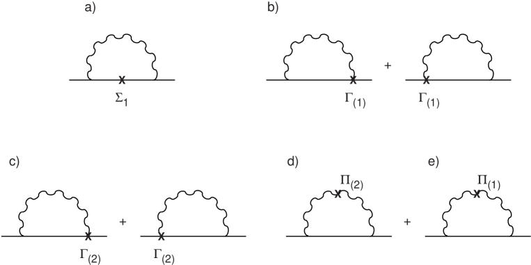
Figure 3:  One-loop subtraction diagrams. The vertex factors for “$\times$” are minus the divergent parts of the indicated one-loop amplitudes $\Sigma_{1},\,\Gamma_{(1)}$, etc.

Figure 4: One-particle-reducible quark self-energy diagrams. The vertex factor for $\times$ is given by [$-$ divergent part of $\Sigma_{1}$.]

The one-loop amplitudes $\Sigma_{1},\,\Gamma_{(1)},\,\Gamma_{(2)},\,\Pi_{(2)}$, and $\Pi_{(1)}$ are of order $g^{2}$, so that the amplitudes of Figures 3a to 3e are all of order $g^{4}$. These amplitudes belong, therefore, to $\Sigma_{2}$, along with the amplitudes of Figures 1a to 1e, of course. In principle, the amplitudes of the one-particle-reducible diagrams (Figure 4) also contribute to $\Sigma_{2}$, but it is easy to see that the divergent parts of these amplitudes cancel completely with one another, due to the factorizability of all four integrals.

All of the diagrams of Figures 3 and 1a to 1e contribute nonlocal divergences to $\Sigma_{2}$; however, the nonlocal contributions from Figs. 1a to 1e are exactly cancelled by the nonlocal parts from the corresponding diagrams of Figure 3, as expected on theoretical grounds [9, 23, 24].

4.2 Two-loop Counterterms

The divergent parts of the amplitudes for Figures 1a to 1e and 3a to 3e are shown in Table 1, excluding the nonlocal divergent terms which cancel as noted above. To find the local divergent part of the amplitude for a particular figure, one multiplies the numbers in the applicable row of the table by the corresponding factors at the top of the table, then adds the resulting terms together, and multiplies the sum by the color factor at the right-hand end of the row. (We recall that $\,{\textstyle\epsilon}\equiv 2-\omega$, and $\,\widetilde{\alpha}_{s}\equiv g^{2}\Gamma({\textstyle\epsilon})(4\pi)^{-\omega}$ for modified minimal subtraction.) The divergent part of $\Sigma_{2}$ is the sum of the results for all ten figures, as shown in the “total” section at the bottom of the table.

Table 1: Local divergent parts of the amplitudes for Figures 1a to 1e and 3a to 3e. Each number is to be multiplied by the expressions at the top of its column and right-hand end of its row. $C_{F},\,N_{C},\,N_{f}$, and $\,\widetilde{\alpha}_{s}\,$ are defined after Eq. (67). Columns with 1 at the top give double-pole terms; columns with ${\textstyle\epsilon}$, single poles. Vectors are in Minkowski space, and ${\textstyle\epsilon}\equiv 2-\omega$.

		$\stackrel{{\scriptstyle\displaystyle m}}{{\overbrace{\rule{42.0pt}{0.0pt}}}}$		$\stackrel{{\scriptstyle\displaystyle p_{\!}\!\!/}}{{\overbrace{\rule{42.0pt}{0.0pt}}}}$		$\stackrel{{\scriptstyle\displaystyle\frac{n^{*}\!\!\cdot\!p\,n\!\!\!/}{n^{*}\!\!\cdot\!n}}}{{\overbrace{\rule{42.0pt}{0.0pt}}}}$		$\stackrel{{\scriptstyle\displaystyle\frac{n\!\cdot\!p\,n\!\!\!/^{*}}{n^{*}\!\!\cdot\!n}}}{{\overbrace{\rule{42.0pt}{0.0pt}}}}$
Figure		1	${\textstyle\epsilon}$	1	${\textstyle\epsilon}$	1	${\textstyle\epsilon}$	1	${\textstyle\epsilon}$
rainbow	1a	–8	16	–3	–$\frac{3}{2}$	–6	–40	6	8	$\frac{1}{2}i\widetilde{\alpha}_{s}^{2}C_{F}^{2}$
	3a	16	–24	6	2	12	24	–12	–8	$\frac{1}{2}i\widetilde{\alpha}_{s}^{2}C_{F}^{2}$
over-	1b	4	8	4	2	14	60	–6	–12	$\frac{1}{2}i\widetilde{\alpha}_{s}^{2}(C_{F}^{2}-\frac{1}{2}N_{C}C_{F})$
lapping
	3b	–8	0	–8	–4	–28	–40	12	8	$\frac{1}{2}i\widetilde{\alpha}_{s}^{2}(C_{F}^{2}-\frac{1}{2}N_{C}C_{F})$
spider	1c	4	–16	0	–2	–6	–20	–2	4	$\frac{1}{4}i\widetilde{\alpha}_{s}^{2}N_{C}C_{F}$
	3c	–8	0	0	–4	12	24	4	8	$\frac{1}{4}i\widetilde{\alpha}_{s}^{2}N_{C}C_{F}$
gluon-	1d	–$\frac{44}{3}$	–$\frac{124}{9}$	–$\frac{10}{3}$	–$\frac{47}{9}$	$\frac{16}{3}$	$\frac{284}{9}$	$\frac{32}{3}$	$\frac{292}{9}$	$\frac{1}{4}i\widetilde{\alpha}_{s}^{2}N_{C}C_{F}$
bubble
	3d	$\frac{88}{3}$	0	$\frac{20}{3}$	$\frac{44}{3}$	–$\frac{32}{3}$	–$\frac{104}{3}$	–$\frac{64}{3}$	–$\frac{88}{3}$	$\frac{1}{4}i\widetilde{\alpha}_{s}^{2}N_{C}C_{F}$
quark-	1e	$\frac{8}{3}$	$\frac{40}{9}$	$\frac{4}{3}$	$\frac{14}{9}$	$\frac{8}{3}$	$\frac{64}{9}$	–$\frac{8}{3}$	–$\frac{64}{9}$	$\frac{1}{4}i\widetilde{\alpha}_{s}^{2}N_{f}C_{F}$
bubble
	3e	–$\frac{16}{3}$	0	–$\frac{8}{3}$	–$\frac{8}{3}$	–$\frac{16}{3}$	–$\frac{16}{3}$	$\frac{16}{3}$	$\frac{16}{3}$	$\frac{1}{4}i\widetilde{\alpha}_{s}^{2}N_{f}C_{F}$
		–$\frac{8}{3}$	$\frac{40}{9}$	–$\frac{4}{3}$	–$\frac{10}{9}$	–$\frac{8}{3}$	$\frac{16}{9}$	$\frac{8}{3}$	–$\frac{16}{9}$	$\frac{1}{4}i\widetilde{\alpha}_{s}^{2}N_{f}C_{F}$
total $\ \left\{\rule{0.0pt}{32.0pt}\right.\!\!\!\!\!\!\!$		$\frac{44}{3}$	–$\frac{340}{9}$	$\frac{22}{3}$	$\frac{49}{9}$	$\frac{44}{3}$	–$\frac{172}{9}$	–$\frac{44}{3}$	$\frac{172}{9}$	$\frac{1}{4}i\widetilde{\alpha}_{s}^{2}N_{C}C_{F}$
$(\Sigma_{2})$		4	0	–1	–$\frac{3}{2}$	–8	4	0	–4	$\frac{1}{2}i\widetilde{\alpha}_{s}^{2}C_{F}^{2}$

A knowledge of the divergent part of $\Sigma_{2}$ enables us to verify explicitly that the effective quark propagator may indeed be rendered finite at two-loop order by means of the substitutions $\,m\to m-\delta m\,$ and $\,\psi\to\psi+N\psi\,$, as implied by Bassetto, Dalbosco and Soldati. The O$(\widetilde{\alpha}_{s})$ parts of $N$ and $\delta m$ are already shown in Eqs. (71). Multiplying Eq. (59) by $S^{-1}$ from the left and by $(S_{\mathrm{e}ff})^{-1}$ from the right, then solving for $(S_{\mathrm{e}ff})^{-1}$ and replacing $S$ by $S_{\mathrm{r}en}$, we get

$$(S_{\mathrm{e}ff})^{-1}\,=\,(S_{\mathrm{r}en})^{-1}-i\Sigma_{1}-i\Sigma_{2}-\dots\!.$$ (72)

To keep $S_{\mathrm{e}ff}$ finite at two-loop order, we must ensure that the divergent parts of $\Sigma_{2}$ in Eq. (72) are cancelled by terms from $(S_{\mathrm{r}en})^{-1}$; the latter depends on $N$ and $\delta m$, as seen from Eq. (68). (The divergent parts of $\Sigma_{1}$ cancel already, thanks to the particular choice of the O$(\widetilde{\alpha}_{s})$ parts of $N$ and $\delta m$.) Inverting and expanding the right-hand side of (68), we obtain

$$(S_{\mathrm{r}en})^{-1}\,=\,S^{-1}+\delta m+(\delta m-m)\Big{(}N^{*}+N+N^{*}N\Big{)}+N^{*}p_{\!}\!\!/N+N^{*}p_{\!}\!\!/+p_{\!}\!\!/N,\ \$$ (73)

where $\,N^{*}\equiv\gamma^{0}N^{\dagger}\gamma^{0}$. Comparison of the terms of this expansion with the expressions at the tops of the columns in Table 1 suggests that the O$(\widetilde{\alpha}_{s}^{2})$ parts of $N$ and $\delta m$ should be similar in form to the O$(\widetilde{\alpha}_{s})$ parts shown in Eqs. (71). Therefore, let us try the ansatz

$$\delta m\,=\,3m\widetilde{\alpha}_{s}C_{F}+m\widetilde{\alpha}_{s}^{2}C_{F}W\ +{\mathrm{O}}(\widetilde{\alpha}_{s}^{3}),$$ (74)

and

$$N\,=\,\widetilde{\alpha}_{s}C_{F}\left(\frac{n\!\!\!/^{*}n\!\!\!/}{n^{*}\!\!\cdot\!n}-\frac{1}{2}\right)+\widetilde{\alpha}_{s}^{2}C_{F}\left(X\frac{n\!\!\!/^{*}n\!\!\!/}{n^{*}\!\!\cdot\!n}+Y\right)\ +{\mathrm{O}}(\widetilde{\alpha}_{s}^{3}),$$ (75)

and then see if we can find expressions for $W,\,X$, and $Y$ that will cause all O$(\widetilde{\alpha}_{s}^{2})$ terms in Eq. (72) to cancel.

Substituting from Eqs. (74) and (75) into Eq. (73), and applying the light-cone condition $\,n^{2}=n^{*2}=0$, we find that the noncovariant O$(\widetilde{\alpha}_{s}^{2})$ part of $(S_{\mathrm{r}en})^{-1}$ reads

$$\widetilde{\alpha}_{s}^{2}C_{F}\left[(2X-C_{F})\frac{n^{*}\!\!\cdot\!p\,n\!\!\!/-n\!\cdot\!p\,n\!\!\!/^{*}}{n^{*}\!\!\cdot\!n}+4C_{F}\frac{n^{*}\!\!\cdot\!p\,n\!\!\!/}{n^{*}\!\!\cdot\!n}\right].$$ (76)

$S_{\mathrm{e}ff}$ can be finite only if there is some value of $X$ that makes expression (76) match the noncovariant, divergent part of $i\Sigma_{2}$. Such a match is possible, but only because the coefficients under $n^{*}\!\!\cdot\!p\,n\!\!\!/$ in the “total” part of Table 1 are the negatives of the corresponding coefficients under $n\!\cdot\!p\,n\!\!\!/^{*}$, except for the last two double-pole coefficients in the last row. These last double-pole coefficients give rise to a term which cancels with the last term in brackets in (76). This term in (76) derives purely from the leading term of $N$, via the $N^{*}p_{\!}\!\!/N$ term in Eq. (73), so its coefficient cannot be adjusted (unlike $X$) to make it cancel with some arbitrary term from $i\Sigma_{2}$. Consequently, the anti-symmetry between the coefficients of $n^{*}\!\!\cdot\!p\,n\!\!\!/$ and $n\!\cdot\!p\,n\!\!\!/^{*}$ in $\Sigma_{2}$ must be broken in exactly the way that we have found it to be broken, otherwise the BDS scheme would have failed.

To complete our derivation of $N$ and $\delta m$, having substituted from Eqs. (74) and (75) into Eq. (73), we then substitute from Eq. (73) and Table 1 into Eq. (72), and set the total of the O$(\widetilde{\alpha}_{s}^{2})$ terms on the right to zero. In this way we find the following expressions for $W$, $X$, and $Y$:

$$W\! = \!\frac{N_{f}}{4}\left(4-\frac{10}{3}{\textstyle\epsilon}\right)+\frac{N_{C}}{4}\left(-22+\frac{97}{3}{\textstyle\epsilon}\right)+\frac{C_{F}}{2}\left(-9+\frac{3}{2}{\textstyle\epsilon}\right),$$ (77)

$$X\! = \!\frac{N_{f}}{4}\left(\frac{4}{3}-\frac{8}{9}{\textstyle\epsilon}\right)+\frac{N_{C}}{4}\left(-\frac{22}{3}+\frac{86}{9}{\textstyle\epsilon}\right)+\frac{C_{F}}{2}\left(1-2{\textstyle\epsilon}\right),$$ (78)

$$Y\! = \!\frac{N_{f}}{4}\left(-\frac{2}{3}+\frac{13}{9}{\textstyle\epsilon}\right)+\frac{N_{C}}{4}\left(\frac{11}{3}-\frac{221}{18}{\textstyle\epsilon}\right)+\frac{C_{F}}{2}\left(\frac{1}{4}+\frac{11}{4}{\textstyle\epsilon}\right).$$ (79)

Thus we have confirmed the claim of Bassetto, Dalbosco, and Soldati for the two-loop quark self-energy function. It is also significant to realize that the mass counterterm $\delta m$ in the light-cone gauge, Eq. (74), is exactly the same as in the general linear covariant gauge [22], at least up to two-loop order. This result is a reassuring reflection of the gauge symmetry of QCD [25].

5 Conclusion

In this paper, we have evaluated the complete quark propagator to two-loop order, and demonstrated for the first time its renormalizability in the noncovariant light-cone gauge. The chief technical tool in this three-year project was the powerful matrix integration technique which had been exploited in our first paper [4] to evaluate the divergent part of the overlapping self-energy function (see Fig. 1b in the present article). Now, three years later, we have finally succeeded in computing, without approximation, the divergent parts of the four remaining two-loop diagrams in the quark propagator, namely: the quark-bubble diagram (Fig. 1e), the rainbow diagram (Fig. 1a), the spider diagram (Fig. 1c), and the gluon-bubble diagram (Fig. 1d), along with their counterterm graphs, depicted in Figs. 3e, 3a, 3c and 3d, respectively.

Other technical tools, apart from the matrix method and a reliable computer algebra program, included dimensional regularization, the $n^{*}_{\mu}$-prescription for the spurious poles of $(q\!\cdot\!n)^{-1}$ ($n^{2}=0$), as well as a detailed analysis of the boundary singularities in five- and even six-dimensional parameter space.

The divergent part of the total two-loop correction $\Sigma_{2}$ to the quark propagator can be read off from Table 1, and has the form

$$\Sigma_{2}\ = \ i\widetilde{\alpha}^{2}_{s}\left\{C_{F}^{2}\left(2m-\frac{p_{\!}\!\!/}{2}-4\,{n^{*}\!\!\cdot\!p\,n\!\!\!/\over n^{*}\!\!\cdot\!n}\right)\right.$$ (80)

$$\ \ \left.\qquad+~{}\left(\frac{11}{3}N_{C}-\frac{2}{3}N_{f}\right)C_{F}\left(m+\frac{1}{2}p_{\!}\!\!/+{n^{*}\!\!\cdot\!p\,n\!\!\!/-n\!\cdot\!p\,n\!\!\!/^{*}\over n^{*}\!\!\cdot\!n}\right)\right\}$$

$$+~{}i\widetilde{\alpha}_{s}^{2}\,{\textstyle\epsilon}\left\{C_{F}^{2}\left(-\frac{3}{4}p_{\!}\!\!/+2\left[{n^{*}\!\!\cdot\!p\,n\!\!\!/-n\!\cdot\!p\,n\!\!\!/^{*}\over n^{*}\!\!\cdot\!n}\right]\right)\right.$$

$$\qquad\qquad+~{}\frac{N_{C}C_{F}}{9}\left(-85m+\frac{49}{4}p_{\!}\!\!/-43\left[{n^{*}\!\!\cdot\!p\,n\!\!\!/-n\!\cdot\!p\,n\!\!\!/^{*}\over n^{*}\!\!\cdot\!n}\right]\right)$$

$$\left.\qquad\qquad+~{}\frac{N_{f}C_{F}}{9}\left(10m-\frac{5}{2}p_{\!}\!\!/+4\left[{n^{*}\!\!\cdot\!p\,n\!\!\!/-n\!\cdot\!p\,n\!\!\!/^{*}\over n^{*}\!\!\cdot\!n}\right]\right)\right\},$$

with $\widetilde{\alpha}_{s}\equiv g^{2}\Gamma({\textstyle\epsilon})(4\pi)^{{\textstyle\epsilon}-2}$. The expression (80) has several noteworthy features:

• The anti-symmetry between the coefficients of $n^{*}\!\!\cdot\!pn\!\!\!/$ and $n\!\cdot\!pn\!\!\!/^{*}$ (proportional to $\widetilde{\alpha}^{2}_{s}C_{F}^{2})$ is identical to the anti-symmetry predicted by the Bassetto-Dalbosco-Soldati renormalization scheme [10].

• The divergent part of $\Sigma_{2}$ is a local function of the external momentum $p$, even off mass-shell, since all nonlocal divergent terms cancel exactly. Notice that $\Sigma_{2}$ contains both covariant and noncovariant components.

• The structure of $\Sigma_{2}$ implies the quark mass counterterm $\delta m$,

  $$\delta m\,=\,3m\widetilde{\alpha}_{s}\,C_{F}+m\widetilde{\alpha}^{2}_{s}\,C_{F}\,W+{\mathrm{O}}(\widetilde{\alpha}^{3}_{s})\,,$$ (81)

  which is gauge-independent, as expected ($W$ is given by Eq. (77)). It is both interesting, and re-assuring from a calculational point of view, that the mass counterterm in the noncovariant light-cone gauge is exactly the same as in the general linear covariant gauge [22] – at least to two-loop order.

• The factor $N$ for the renormalization of the quark field $\psi$ is likewise local, albeit gauge-dependent:

  $$N\,=\,\widetilde{\alpha}_{s}\,C_{F}\left({n\!\!\!/^{*}n\!\!\!/\over n^{*}\!\!\cdot\!n}-{1\over 2}\right)+\widetilde{\alpha}^{2}_{s}\,C_{F}\left(X{n\!\!\!/^{*}n\!\!\!/\over n^{*}\!\!\cdot\!n}-Y\right)+{\mathrm{O}}(\widetilde{\alpha}^{3}_{s})\,,$$ (82)

  with $X$ and $Y$ defined in Eqs. (78) and (79), respectively.

The cancellation of nonlocal divergences, the consistency of our results with the Bassetto-Dalbosco-Soldati renormalization scheme, and the agreement between our mass renormalization and the two-loop covariant result all serve to demonstrate the reliability of the matrix integration method, as well as the validity, at two-loop order, of the $n^{*}_{\mu}$-prescription for the unphysical poles of the light-cone gauge propagator.

Since physically meaningful predictions can only be made with a theory whose divergences have been subtracted consistently, our result will help to make the light-cone gauge a more useful tool for practical two-loop calculations in QCD and other non-Abelian theories. Complete two-loop renormalization will also allow the computation of certain three-loop quantities, by means of renormalization group improvements [26].

Of course, the cancellation of the divergences in the effective quark propagator is only part of the overall renormalization picture. In order to complete the two-loop renormalization of light-cone QCD, we must also find the counterterms which eliminate the two-loop divergences from the effective gluon propagator and vertex factors. We should be able to find these new counterterms using the same methods that have worked in this paper for the renormalization of the quark propagator.

Appendix

The tables in this Appendix show one possible way in which the integrals $I_{\mathrm{a}}$ to $I_{\mathrm{e}}$ from Subsection 2.2 may be broken down into simpler integrals. Specifically, if we regard the columns of the tables as Cartesian vectors, then $I_{\mathrm{a}}$, for example, is the sum over all five tables of the dot product of the column headed by $I_{\mathrm{a}}$ (if any), times the integral over $q$ and $k$ of the “integrand” column (plus some finite integrals which have been discarded). Blank spaces in the tables denote zeros. For example,

$$I_{\mathrm{c}}\,=\,4\int\frac{n\!\!\!/n\!\cdot\!p\,{\mathrm{d}}^{2\omega}q\,{\mathrm{d}}^{2\omega}k}{\mathsf{n}qQx\ o}+2{\textstyle\epsilon}\int\frac{n\!\!\!/\,{\mathrm{d}}^{2\omega}q\,{\mathrm{d}}^{2\omega}k}{\mathsf{n}\ \ xKk}+\dots\!.$$

The symbols in the denominators of the integrands are to be decoded as follows:

$${\mathsf{n}}\to n\!\cdot\!q,\ {\mathsf{q}}\to q^{2},\qquad{\mathsf{Q}}\to[(p-q)^{2}+m^{2}],\qquad{\mathsf{x}}\to[(p-q-k)^{2}+m^{2}],$$

$${\mathsf{o}}\to n\!\cdot\!k,\ {\mathsf{k}}\to k^{2},\qquad{\mathsf{K}}\to[(p-k)^{2}+m^{2}],\qquad{\mathsf{y}}\to(q-k)^{2}.$$

Note that all 4-vectors in this Appendix are in Euclidean space.

For each row of each table, the divergent part of the integral over $q$ and $k$ of the expression in the “integrand” column is $\,\pi^{2\omega}\Gamma(2{\textstyle\epsilon})(m^{2}+p^{2})^{-2{\textstyle\epsilon}}\,$ times the expression in the final column, where $\,{\textstyle\epsilon}\equiv 2-\omega$, and

$$b\equiv\frac{m^{2}}{p^{2}}\ln\left(\frac{m^{2}+p^{2}}{m^{2}}\right)-1,\qquad\qquad\ n_{p}\equiv\frac{n^{*}\!\!\cdot\!p}{n^{*}\!\!\cdot\!n}n,\qquad\quad\ n_{p}^{*}\equiv\frac{n\!\cdot\!p}{n^{*}\!\!\cdot\!n}n^{*},$$

$$c\equiv\left(2+\frac{m^{2}}{p^{2}}\right)b,\ \ \qquad\qquad h\!\!\!/\equiv(b-f)\left(\frac{p^{2}n\!\!\!/}{2n\!\cdot\!p}-p_{\!}\!\!/\right)-fn\!\!\!/_{p}^{*}-n\!\!\!/_{p}+un\!\!\!/,$$

$$f\equiv\frac{m^{2}+p_{\|}^{2}}{p_{\perp}^{2}}\ln\left(\frac{m^{2}+p^{2}}{m^{2}+p_{\|}^{2}}\right)-1,\qquad\qquad t\equiv\frac{fn^{*}\!\!\cdot\!p}{n^{*}\!\!\cdot\!n}+\frac{(b-f)p^{2}}{2n\!\cdot\!p},$$

$$a_{\mu}\equiv\frac{m^{2}p_{\perp\mu}}{p_{\perp}^{2}}\ln\left(\frac{m^{2}+p^{2}}{m^{2}+p_{\|}^{2}}\right),\qquad\qquad p_{\|}=n_{p}+n_{p}^{*},\qquad\quad p_{\perp}\equiv p-p_{\|},$$

$$u\equiv\frac{(m^{2}+p^{2})d}{2n\!\cdot\!p},\,\ \qquad\qquad\qquad d\equiv{\mathrm{L}i}_{2}\left(\frac{p^{2}}{m^{2}+p^{2}}\right)-{\mathrm{L}i}_{2}\left(\frac{p_{\perp}^{2}}{m^{2}+p^{2}}\right),$$

$$v\equiv\frac{m^{2}d}{n\!\cdot\!p},\ \qquad\qquad{\mathrm{L}i}_{2}(z)\equiv\int_{0}^{1}\frac{\ln\tau\ {\mathrm{d}}\tau}{\tau-1/z}\ \quad{\mathrm{(}the\ ``dilogarithm")}.$$

$$\begin{array}[]{ |@{\,} c @{\,}|@{\,} c @{\,}|@{\,} c @{\,}| r @{/} l | l }I_{\mathrm{a}}&I_{\mathrm{b}}&I_{\mathrm{c}}&\lx@intercol\hfil{\mathrm{i}ntegrand},\ R\hfil\lx@intercol\vrule\lx@intercol&\displaystyle\frac{(m^{2}+p^{2})^{2{\textstyle\epsilon}}\!\!\!\!}{\pi^{2\omega}\Gamma(2{\textstyle\epsilon})}\,\cdot\,{\mathrm{d}iv\!.part}\!\int\!R\,{\mathrm{d}}^{2\omega}q\,{\mathrm{d}}^{2\omega}k\\ \hline\cr\hline\cr-4&&&m^{2}n\!\!\!/&\mathsf{n}qQx\ k&2vn\!\!\!/\\ \hline\cr 2&-4&4&n\!\!\!/n\!\cdot\!p&\mathsf{n}qQx\ \ o&4(1+b+d)n\!\!\!/_{p}-4(t+u)n\!\!\!/\\ &4&&n\!\!\!/n\!\cdot\!p&\mathsf{n}qQ\ K\ o&4dn\!\!\!/_{p}\\ \hline\cr-2{\textstyle\epsilon}&2{\textstyle\epsilon}&2{\textstyle\epsilon}&n\!\!\!/&\mathsf{n}\ \ xKk&(\frac{1}{{\textstyle\epsilon}}+4-4b+2c)n\!\!\!/_{p}\\ 2&-2-2{\textstyle\epsilon}&-2&n\!\!\!/&\mathsf{n}\ Qx\ k&(\frac{2}{{\textstyle\epsilon}}+4)n\!\!\!/_{p}-4tn\!\!\!/\\ &-2{\textstyle\epsilon}&-2{\textstyle\epsilon}&n\!\!\!/&\mathsf{n}\ Q\ Kk&(\frac{4}{{\textstyle\epsilon}}+4-4b)n\!\!\!/_{p}-4tn\!\!\!/\\ \hline\cr&-4+4{\textstyle\epsilon}&-4+4{\textstyle\epsilon}&n\!\!\!/q\!\cdot\!k&\mathsf{n}qQ\ Kk&(\frac{1}{{\textstyle\epsilon}}-c)n\!\!\!/_{p}+(u-t)n\!\!\!/\\ \hline\cr 4-4{\textstyle\epsilon}&&&n\!\!\!/p\!\cdot\!k&\mathsf{n}qQx\ k&(-\frac{1}{2{\textstyle\epsilon}}-\frac{1}{2})n\!\!\!/_{p}+(t+u-v)n\!\!\!/\\ \hline\cr 4&&&n\!\!\!/p\!\cdot\!q&\mathsf{n}q\ xKk&(\frac{1}{{\textstyle\epsilon}}+3-2b)n\!\!\!/_{p}\\ &-4&&n\!\!\!/p\!\cdot\!q&\mathsf{n}\ QxKk&(\frac{1}{{\textstyle\epsilon}}+3-2b)n\!\!\!/_{p}\\ \hline\cr 8-8{\textstyle\epsilon}&-4+4{\textstyle\epsilon}&-8+8{\textstyle\epsilon}&k\!\!\!/n\!\cdot\!k&\mathsf{n}q\ xKk&-\frac{5}{8}p_{\!}\!\!/+\frac{1}{4}n\!\!\!/_{p}-\frac{3}{4}n\!\!\!/_{p}^{*}\\ &-4+4{\textstyle\epsilon}&&k\!\!\!/n\!\cdot\!k&\mathsf{n}\ QxKk&-\frac{3}{8}p_{\!}\!\!/+(\frac{1}{2{\textstyle\epsilon}}+\frac{3}{4})n\!\!\!/_{p}-tn\!\!\!/-\frac{3}{4}n\!\!\!/_{p}^{*}\\ \hline\cr&&&\lx@intercol\hfil\hfil\lx@intercol\vrule\lx@intercol&\\[-18.0pt] &4-4{\textstyle\epsilon}&&\lx@intercol\hfil\displaystyle\frac{(m^{2}+p^{2})k\!\!\!/n\!\cdot\!k}{\mathsf{n}qQxKk}\hfil\lx@intercol&un\!\!\!/\\[-18.0pt] &&&\lx@intercol\hfil\hfil\lx@intercol\vrule\lx@intercol&\\ \hline\cr-4{\textstyle\epsilon}&4{\textstyle\epsilon}&4{\textstyle\epsilon}&q\!\!\!/n\!\cdot\!k&\mathsf{n}q\ xKk&-\frac{1}{4}p_{\!}\!\!/+(\frac{1}{2{\textstyle\epsilon}}+1-c)n\!\!\!/_{p}^{*}\\ &4-4{\textstyle\epsilon}&&q\!\!\!/n\!\cdot\!k&\mathsf{n}qQxK&(-\frac{1}{4{\textstyle\epsilon}}-\frac{1}{8}+\frac{1}{2}c)p_{\!}\!\!/+2h\!\!\!/+(\frac{1}{{\textstyle\epsilon}}+3)n\!\!\!/_{p}^{*}\\ 4-4{\textstyle\epsilon}&-8+8{\textstyle\epsilon}&-8+8{\textstyle\epsilon}&q\!\!\!/n\!\cdot\!k&\mathsf{n}qQx\ k&(-\frac{1}{4{\textstyle\epsilon}}-\frac{3}{8}+\frac{1}{2}c)p_{\!}\!\!/+h\!\!\!/+(\frac{1}{2{\textstyle\epsilon}}+\frac{3}{2})n\!\!\!/_{p}^{*}\\ &4-4{\textstyle\epsilon}&4-4{\textstyle\epsilon}&q\!\!\!/n\!\cdot\!k&\mathsf{n}qQ\ Kk&h\!\!\!/+(\frac{1}{{\textstyle\epsilon}}+1-c)n\!\!\!/_{p}^{*}\\ \hline\cr-16+8{\textstyle\epsilon}&-4+4{\textstyle\epsilon}&24-8{\textstyle\epsilon}&k\!\!\!/n\!\cdot\!p&\mathsf{n}q\ xKk&-n\!\!\!/_{p}^{*}\\ &20-8{\textstyle\epsilon}&&k\!\!\!/n\!\cdot\!p&\mathsf{n}\ QxKk&-n\!\!\!/_{p}^{*}\\ &-4+4{\textstyle\epsilon}&-4+4{\textstyle\epsilon}&k\!\!\!/n\!\cdot\!p&\mathsf{n}qQx\ k&dp_{\!}\!\!/-h\!\!\!/-(\frac{1}{2{\textstyle\epsilon}}+\frac{3}{2})n\!\!\!/_{p}^{*}\\ &4-4{\textstyle\epsilon}&4-4{\textstyle\epsilon}&k\!\!\!/n\!\cdot\!p&\mathsf{n}qQ\ Kk&dp_{\!}\!\!/\\ \hline\cr 4{\textstyle\epsilon}&4-4{\textstyle\epsilon}&4-4{\textstyle\epsilon}&q\!\!\!/n\!\cdot\!p&\mathsf{n}q\ xKk&(\frac{1}{{\textstyle\epsilon}}+3-2b)n\!\!\!/_{p}^{*}\\ &-4&&q\!\!\!/n\!\cdot\!p&\mathsf{n}\ QxKk&(\frac{1}{{\textstyle\epsilon}}+3-2b)n\!\!\!/_{p}^{*}\\ &4+8{\textstyle\epsilon}&&q\!\!\!/n\!\cdot\!p&\mathsf{n}qQxK&2h\!\!\!/+(\frac{1}{{\textstyle\epsilon}}+3)n\!\!\!/_{p}^{*}\\ -8&4-4{\textstyle\epsilon}&4&q\!\!\!/n\!\cdot\!p&\mathsf{n}qQx\ k&2h\!\!\!/+(\frac{1}{{\textstyle\epsilon}}+3)n\!\!\!/_{p}^{*}\\ &-4+4{\textstyle\epsilon}&-4+4{\textstyle\epsilon}&q\!\!\!/n\!\cdot\!p&\mathsf{n}qQ\ Kk&2h\!\!\!/+(\frac{2}{{\textstyle\epsilon}}+4-2b)n\!\!\!/_{p}^{*}\\ \hline\cr\hline\cr\end{array}$$

$$\begin{array}[]{ | c | c | c | r @{/} l | l }I_{\mathrm{a}}&I_{\mathrm{b}}&I_{\mathrm{c}}&\lx@intercol\hfil{\mathrm{i}ntegrand},\ R\hfil\lx@intercol\vrule\lx@intercol&\displaystyle\frac{(m^{2}+p^{2})^{2{\textstyle\epsilon}}\!\!\!\!}{\pi^{2\omega}\Gamma(2{\textstyle\epsilon})}\,\cdot\,{\mathrm{d}iv\!.part}\!\int\!R\\ \hline\cr\hline\cr 8{\textstyle\epsilon}p_{\!}\!\!/+&8(1-{\textstyle\epsilon})p_{\!}\!\!/+&-16{\textstyle\epsilon}p_{\!}\!\!/+&\lx@intercol\hfil\hfil\lx@intercol\vrule\lx@intercol\\[-14.0pt] &&&n\!\cdot\!k&\mathsf{n}q\ xKk&-1\\[-14.0pt] 8({\textstyle\epsilon}-1)m&8(1-{\textstyle\epsilon})m&16(1-{\textstyle\epsilon})m&\lx@intercol\hfil\hfil\lx@intercol\vrule\lx@intercol\\ \hline\cr&4m-4p_{\!}\!\!/&&n\!\cdot\!k&\mathsf{n}\ QxKk&-1\\ \hline\cr&8(1-{\textstyle\epsilon})p_{\!}\!\!/+&8(1-{\textstyle\epsilon})p_{\!}\!\!/+&\lx@intercol\hfil\hfil\lx@intercol\vrule\lx@intercol\\[-14.0pt] &&&n\!\cdot\!k&\mathsf{n}qQx\ k&-\frac{1}{2{\textstyle\epsilon}}-\frac{3}{2}+b+d\\[-14.0pt] &8(1-{\textstyle\epsilon})m&8(1-{\textstyle\epsilon})m&\lx@intercol\hfil\hfil\lx@intercol\vrule\lx@intercol\\ \hline\cr&8({\textstyle\epsilon}-1)p_{\!}\!\!/+&8({\textstyle\epsilon}-1)p_{\!}\!\!/+&\lx@intercol\hfil\hfil\lx@intercol\vrule\lx@intercol\\[-14.0pt] &&&n\!\cdot\!k&\mathsf{n}qQ\ Kk&d\\[-14.0pt] &8({\textstyle\epsilon}-1)m&8({\textstyle\epsilon}-1)m&\lx@intercol\hfil\hfil\lx@intercol\vrule\lx@intercol\\ \hline\cr\hline\cr&2(2-{\textstyle\epsilon})p_{\!}\!\!/+&4({\textstyle\epsilon}-1)p_{\!}\!\!/+&\lx@intercol\hfil\hfil\lx@intercol\vrule\lx@intercol\\[-14.0pt] &&&\ 1&\mathsf{q}\ xKk&\frac{1}{{\textstyle\epsilon}}+3-2b\\[-14.0pt] &2(1-{\textstyle\epsilon})m&4{\textstyle\epsilon}m&\lx@intercol\hfil\hfil\lx@intercol\vrule\lx@intercol\\ \hline\cr&8(1-{\textstyle\epsilon})p_{\!}\!\!/+&&\lx@intercol\hfil\hfil\lx@intercol\vrule\lx@intercol\\[-14.0pt] &&&\ 1&\mathsf{q}QxK&\frac{1}{{\textstyle\epsilon}}+3-2b\\[-14.0pt] &8m&&\lx@intercol\hfil\hfil\lx@intercol\vrule\lx@intercol\\ \hline\cr 4{\textstyle\epsilon}p_{\!}\!\!/+&2(2-{\textstyle\epsilon})p_{\!}\!\!/+&8(1-{\textstyle\epsilon})p_{\!}\!\!/+&\lx@intercol\hfil\hfil\lx@intercol\vrule\lx@intercol\\[-14.0pt] &&&\ 1&\mathsf{q}Qx\ k&\frac{1}{{\textstyle\epsilon}}+3-2b\\[-14.0pt] 8({\textstyle\epsilon}-1)m&2(1-{\textstyle\epsilon})m&8(1-{\textstyle\epsilon})m&\lx@intercol\hfil\hfil\lx@intercol\vrule\lx@intercol\\ \hline\cr&2({\textstyle\epsilon}-2)p_{\!}\!\!/+&-2(1+{\textstyle\epsilon})p_{\!}\!\!/&\lx@intercol\hfil\hfil\lx@intercol\vrule\lx@intercol\\[-14.0pt] &&&\ 1&\mathsf{q}Q\ Kk&\frac{2}{{\textstyle\epsilon}}+4-4b\\[-14.0pt] &2({\textstyle\epsilon}-1)m&-2{\textstyle\epsilon}m&\lx@intercol\hfil\hfil\lx@intercol\vrule\lx@intercol\\ \hline\cr-4{\textstyle\epsilon}&4-4{\textstyle\epsilon}&4-4{\textstyle\epsilon}&q\!\!\!/&\mathsf{q}\ xKk&(\frac{1}{4{\textstyle\epsilon}}+\frac{9}{8}-b+\frac{1}{2}c)p_{\!}\!\!/\\ &-8+8{\textstyle\epsilon}&&q\!\!\!/&\mathsf{\ }QxKk&(\frac{3}{4{\textstyle\epsilon}}+\frac{23}{8}-2b+\frac{1}{2}c)p_{\!}\!\!/\\ &-8+4{\textstyle\epsilon}&&q\!\!\!/&\mathsf{q}QxK&(\frac{1}{2{\textstyle\epsilon}}+\frac{1}{4}-c)p_{\!}\!\!/\\ 8-4{\textstyle\epsilon}&-8&-8+4{\textstyle\epsilon}&q\!\!\!/&\mathsf{q}Qx\ k&(\frac{1}{2{\textstyle\epsilon}}+\frac{3}{4}-c)p_{\!}\!\!/\\ &4-4{\textstyle\epsilon}&4-4{\textstyle\epsilon}&q\!\!\!/&\mathsf{q}Q\ Kk&(\frac{1}{{\textstyle\epsilon}}+1-b-c)p_{\!}\!\!/\\ \hline\cr 4-8{\textstyle\epsilon}&&&\ q\!\!\!/&\mathsf{q}QQx&-(2-2b+2c)p_{\!}\!\!/\\ -8+8{\textstyle\epsilon}&&&m^{2}q\!\!\!/&\mathsf{q}QQx\ k&(2-2b+2c)p_{\!}\!\!/\\ -4+8{\textstyle\epsilon}&&&\ m&\mathsf{q}QQx&-(2+2b)m\\ 8-8{\textstyle\epsilon}&&&\ m^{3}&\mathsf{q}QQx\ k&(2+2b)m\\ \hline\cr\hline\cr\end{array}$$

$$\begin{array}[]{ | c | c | c | r @{/} l | l }I_{\mathrm{a}}&I_{\mathrm{b}}&I_{\mathrm{c}}&\lx@intercol\hfil{\mathrm{i}ntegrand},\ R\hfil\lx@intercol\vrule\lx@intercol&\displaystyle\frac{(m^{2}+p^{2})^{2{\textstyle\epsilon}}\!\!\!\!}{\pi^{2\omega}\Gamma(2{\textstyle\epsilon})}\,\cdot\,{\mathrm{d}iv\!.part}\!\int\!R\\ \hline\cr\hline\cr-4&&-8&n\!\!\!/\,n\!\cdot\!p\,p\!\cdot\!k&\mathsf{n}qQx\ ko&2dn\!\!\!/_{p}\\ \hline\cr&2+4{\textstyle\epsilon}&&(m^{2}+p^{2})n\!\!\!/&\mathsf{n}qQxK&4un\!\!\!/\\ -2&-2+2{\textstyle\epsilon}&-2+4{\textstyle\epsilon}&(m^{2}+p^{2})n\!\!\!/&\mathsf{n}qQx\ k&4un\!\!\!/\\ &4-4{\textstyle\epsilon}&4-4{\textstyle\epsilon}&(m^{2}+p^{2})n\!\!\!/&\mathsf{n}qQ\ Kk&4un\!\!\!/\\ \hline\cr-4+4{\textstyle\epsilon}&&&q\!\!\!/n\!\cdot\!p&\mathsf{n}qQQx&-(2+2b)p_{\!}\!\!/+2a\!\!\!/+vn\!\!\!/\\ 8&&&m^{2}q\!\!\!/n\!\cdot\!p&\mathsf{n}qQQx\ k&(2+2b)p_{\!}\!\!/-2a\!\!\!/-vn\!\!\!/\\ \hline\cr 2-2{\textstyle\epsilon}&&&n\!\!\!/&\mathsf{n}\ QQx&2\Big{[}a\!\cdot\!p-(b+1)p^{2}\Big{]}n\!\!\!//n\!\cdot\!p\\ -4&&&m^{2}n\!\!\!/&\mathsf{n}\ QQx\ k&2\Big{[}(b+1)p^{2}-a\!\cdot\!p\Big{]}n\!\!\!//n\!\cdot\!p\\ -2+2{\textstyle\epsilon}&&&(m^{2}+p^{2})n\!\!\!/&\mathsf{n}qQQx&2\Big{[}a\!\cdot\!p-(b+1)p^{2}\Big{]}n\!\!\!//n\!\cdot\!p\\ 4&&&m^{2}(m^{2}+p^{2})n\!\!\!/&\mathsf{n}qQQx\ k&2\Big{[}(b+1)p^{2}-a\!\cdot\!p\Big{]}n\!\!\!//n\!\cdot\!p\\ \hline\cr\hline\cr\end{array}$$

$$\begin{array}[]{ | c | c | r @{/} l | l }I_{\mathrm{d}}&I_{\mathrm{e}}&\lx@intercol\hfil{\mathrm{i}ntegrand},\ R\hfil\lx@intercol\vrule\lx@intercol&\displaystyle\frac{(m^{2}+p^{2})^{2{\textstyle\epsilon}}\!\!\!\!}{\pi^{2\omega}\Gamma(2{\textstyle\epsilon})}\,\cdot\,{\mathrm{d}iv\!.part}\!\int\!R\\ \hline\cr\hline\cr 16{\textstyle\epsilon}p_{\!}\!\!/+&4{\textstyle\epsilon}p_{\!}\!\!/+&\lx@intercol\hfil\hfil\lx@intercol\vrule\lx@intercol\\[-14.0pt] &&\ 1&\mathsf{q}Qy\ k&\frac{1}{{\textstyle\epsilon}}+3-2b\\[-14.0pt] 16({\textstyle\epsilon}-1)m&4({\textstyle\epsilon}-1)m&\lx@intercol\hfil\hfil\lx@intercol\vrule\lx@intercol\\ \hline\cr 8(1-{\textstyle\epsilon})p_{\!}\!\!/+&8p_{\!}\!\!/+&\lx@intercol\hfil\hfil\lx@intercol\vrule\lx@intercol\\[-14.0pt] &&n\!\cdot\!k(n\!\cdot\!q-n\!\cdot\!k)&\mathsf{n}nqQy\ k&\frac{1}{6{\textstyle\epsilon}}+\frac{4}{9}-\frac{1}{3}b\\[-14.0pt] 8(1-{\textstyle\epsilon})m&8m&\lx@intercol\hfil\hfil\lx@intercol\vrule\lx@intercol\\ \hline\cr&&\lx@intercol\hfil\hfil\lx@intercol\vrule\lx@intercol&(\frac{1}{12{\textstyle\epsilon}}+\frac{11}{36})(n\!\!\!/^{*}_{p}-p_{\!}\!\!/)\\[-13.0pt] 16-16{\textstyle\epsilon}&16&p\!\cdot\!k(k\!\!\!/n\!\cdot\!q-q\!\!\!/n\!\cdot\!k)&\mathsf{n}qqQy\ k&\\[-12.0pt] &&\lx@intercol\hfil\hfil\lx@intercol\vrule\lx@intercol&\quad+\ \frac{1}{6}bp_{\!}\!\!/+\frac{1}{6}h\!\!\!/\\ \hline\cr&&\lx@intercol\hfil\hfil\lx@intercol\vrule\lx@intercol&\\[-18.0pt] 8-8{\textstyle\epsilon}&8&\lx@intercol\hfil\displaystyle\frac{(m^{2}+p^{2})n\!\cdot\!k(q\!\!\!/n\!\cdot\!k-k\!\!\!/n\!\cdot\!q)}{\mathsf{n}nqqQy\ k}\hfil\lx@intercol\vrule\lx@intercol&\frac{1}{3}un\!\!\!/\\[8.0pt] \hline\cr\hline\cr\end{array}$$

$$\begin{array}[]{ |@{\,} c @{\,}|@{\,} c @{\,}|@{\,} c @{\,}| r @{/} l | l }I_{\mathrm{c}}&I_{\mathrm{d}}&I_{\mathrm{e}}&\lx@intercol\hfil{\mathrm{i}ntegrand},\ R\hfil\lx@intercol\vrule\lx@intercol&\displaystyle\frac{(m^{2}+p^{2})^{2{\textstyle\epsilon}}\!\!\!\!}{\pi^{2\omega}\Gamma(2{\textstyle\epsilon})}\,\cdot\,{\mathrm{d}iv\!.part}\!\int\!R\,{\mathrm{d}}^{2\omega}q\,{\mathrm{d}}^{2\omega}k\\ \hline\cr\hline\cr&16-16{\textstyle\epsilon}&&mn\!\cdot\!k&\mathsf{n}q\ yKk&m\\ -8+4{\textstyle\epsilon}&&&mn\!\cdot\!k&\mathsf{n}\ QyKk&m\\ \hline\cr-4+12{\textstyle\epsilon}&8-16{\textstyle\epsilon}&4-4{\textstyle\epsilon}&q\!\!\!/&\mathsf{q}Qy\ k&(\frac{1}{2{\textstyle\epsilon}}+\frac{1}{4}-c)p_{\!}\!\!/\\ &-8+8{\textstyle\epsilon}&-8&k\!\!\!/&\mathsf{q}Qy\ k&(\frac{1}{4{\textstyle\epsilon}}+\frac{1}{8}-\frac{1}{2}c)p_{\!}\!\!/\\ \hline\cr 4&-4&&n\!\!\!/&\mathsf{n}\ \ yKk&(\frac{1}{{\textstyle\epsilon}}-2c)n\!\!\!/_{p}\\ 2&4&2&n\!\!\!/&\mathsf{n}\ Qy\ k&(\frac{2}{{\textstyle\epsilon}}+2)n\!\!\!/_{p}-4tn\!\!\!/\\ -2-4{\textstyle\epsilon}&4&&n\!\!\!/&\mathsf{\ }Qy\ ko&2n\!\!\!/_{p}\\ \hline\cr&8&&n\!\!\!/n\!\cdot\!p&\mathsf{n}qQy\ \ o&-4(1+b)n\!\!\!/_{p}+4(t+u)n\!\!\!/\\ \hline\cr&-8&&n\!\!\!/p\!\cdot\!q&\mathsf{n}q\ yKk&(\frac{1}{{\textstyle\epsilon}}+3-2b)n\!\!\!/_{p}\\ 4&&&n\!\!\!/p\!\cdot\!q&\mathsf{n}\ QyKk&(\frac{1}{{\textstyle\epsilon}}+3-2b)n\!\!\!/_{p}\\ \hline\cr 12-12{\textstyle\epsilon}&-16+16{\textstyle\epsilon}&&k\!\!\!/n\!\cdot\!k&\mathsf{n}q\ yKk&\frac{3}{8}p_{\!}\!\!/+\frac{1}{4}n\!\!\!/_{p}+\frac{1}{4}n\!\!\!/^{*}_{p}\\ 4-4{\textstyle\epsilon}&&&k\!\!\!/n\!\cdot\!k&\mathsf{n}\ QyKk&\frac{5}{8}p_{\!}\!\!/+(\frac{1}{2{\textstyle\epsilon}}+\frac{3}{4})n\!\!\!/_{p}-tn\!\!\!/+\frac{1}{4}n\!\!\!/^{*}_{p}\\ &8-8{\textstyle\epsilon}&8&k\!\!\!/n\!\cdot\!k&\mathsf{n}qQy\ k&(\frac{1}{6{\textstyle\epsilon}}+\frac{1}{9}-\frac{1}{3}c)p_{\!}\!\!/-(\frac{1}{6{\textstyle\epsilon}}+\frac{5}{18})n\!\!\!/_{p}+\frac{1}{3}tn\!\!\!/\\ \hline\cr&&&\lx@intercol\hfil\hfil\lx@intercol\vrule\lx@intercol&\\[-18.0pt] -4+4{\textstyle\epsilon}&&&\lx@intercol\hfil\displaystyle\frac{(m^{2}+p^{2})k\!\!\!/n\!\cdot\!k}{\mathsf{n}qQyKk}\hfil\lx@intercol&un\!\!\!/\\[-18.0pt] &&&\lx@intercol\hfil\hfil\lx@intercol\vrule\lx@intercol&\\ \hline\cr&&&\lx@intercol\hfil\hfil\lx@intercol\vrule\lx@intercol&\\[-18.0pt] &-4&-2&\lx@intercol\hfil\displaystyle\frac{(m^{2}+p^{2})n\!\!\!/}{\mathsf{n}qQy\ k}\hfil\lx@intercol&4un\!\!\!/\\[-18.0pt] &&&\lx@intercol\hfil\hfil\lx@intercol\vrule\lx@intercol&\\ \hline\cr 12-12{\textstyle\epsilon}&&&q\!\!\!/n\!\cdot\!k&\mathsf{n}qQy\ k&(\frac{1}{4{\textstyle\epsilon}}+\frac{1}{8}-\frac{1}{2}c)p_{\!}\!\!/\\ -8&8&&q\!\!\!/n\!\cdot\!k&\mathsf{n}q\ yKk&\frac{1}{4}p_{\!}\!\!/+(\frac{1}{2{\textstyle\epsilon}}-c)n\!\!\!/^{*}_{p}\\ \hline\cr&16&&k\!\!\!/n\!\cdot\!p&\mathsf{n}q\ yKk&n\!\!\!/^{*}_{p}\\ -12&&&k\!\!\!/n\!\cdot\!p&\mathsf{n}\ QyKk&n\!\!\!/_{p}^{*}\\ \hline\cr&-8&&q\!\!\!/n\!\cdot\!p&\mathsf{n}q\ yKk&(\frac{1}{{\textstyle\epsilon}}+3-2b)n\!\!\!/^{*}_{p}\\ 4&&&q\!\!\!/n\!\cdot\!p&\mathsf{n}\ QyKk&(\frac{1}{{\textstyle\epsilon}}+3-2b)n\!\!\!/_{p}^{*}\\ &-8&-4&q\!\!\!/n\!\cdot\!p&\mathsf{n}qQy\ k&2h\!\!\!/+(\frac{1}{{\textstyle\epsilon}}+3)n\!\!\!/^{*}_{p}\\ \hline\cr\hline\cr\end{array}$$

References

- [1] G. Leibbrandt, Rev. Mod. Phys. 59, No.4 (1987) 1067.
- [2] G. Leibbrandt, Phys. Rev. D29 (1984) 1699.
- [3] G. Leibbrandt and S.-L. Nyeo, Phys. Lett. B 140 (1984) 417.
- [4] G. Leibbrandt and J. Williams, Nucl. Phys. B440 (1995) 573.
- [5] J. Williams, “Overlapping Two-Loop Quark Self-Energy in the Light-Cone Gauge” (unpublished M.Sc. thesis, University of Guelph, 1994);
-
[6]
A. Smith, Nucl. Phys. B267 (1986) 277;
G. Leibbrandt, Nucl. Phys. B337 (1990) 87. -
[7]
G. Heinrich and Z. Kunszt, Nucl. Phys. B519 (1998) 405
(hep-ph/9708334);
A. Bassetto, G. Heinrich, Z. Kunszt, and W. Vogelsang, Phys. Rev. D58 (1998) 094020 (hep-ph/9805283). - [8] G. ’t Hooft, Nucl. Phys. B33 (1971) 173; 35 (1971) 167.
- [9] J. C. Collins, Renormalization (Cambridge University Press, Cambridge, 1984).
- [10] A. Bassetto, M. Dalbosco, and R. Soldati, Phys. Rev. D36 (1987) 3138.
- [11] A. Bassetto, G. Nardelli, and R. Soldati, Yang-Mills Theories in Algebraic Non-covariant Gauges, (World Scientific, Singapore, 1991).
- [12] G. Leibbrandt, Noncovariant Gauges (World Scientific, Singapore, 1994).
- [13] S.-L. Nyeo, “Renormalization in the Light-Cone Gauge” (unpublished Ph.D. thesis, University of Guelph, 1986).
- [14] J. Frenkel, Phys. Rev. D13 (1976) 2325.
- [15] L. H. Ryder, Quantum Field Theory (Cambridge University Press, Cambridge, 1986).
- [16] S. Mandelstam, Nucl. Phys. B213 (1983) 149.
- [17] A. Bassetto, M. Dalbosco, I. Lazzizzera, and R. Soldati, Phys. Rev. D31 (1985) 2012.
- [18] D. M. Capper and G. Leibbrandt, J. Math. Phys. 15 (1974) 82; 86.
- [19] G. Leibbrandt, Rev. Mod. Phys. 47 (1975) 849.
- [20] S. Weinberg, Phys. Rev. 118 (1960) 838.
-
[21]
E. Mendels, Nuovo Cimento A45 (1978) 87;
A. E. Terrano, Phys. Lett. B93 (1980) 424;
G. Leibbrandt and S.-L. Nyeo, J. Math. Phys. 27 (1986) 627;
A. Bassetto, I. A. Korchemskaya, G. P. Korchemsky, and G. Nardelli, Nucl. Phys. B408 (1993) 62;
F. V. Tkachov, Nucl. Instrum. Meth. A389 (1997) 309 (hep-ph/9609429);
A. I. Davydychev, Acta Phys. Polon. B28 (1997) 841 (hep-ph/9610510), and references therein;
F. V. Tkachov, Sov. J. Part. Nucl. 25 (1994) 649 (hep-ph/9701272);
J. Fleischer, M. Tentyukov, and O. L. Veretin, Acta Phys. Polon. B28 (1997) 2333 (hep-ph/9711437);
A. I. Davydychev and P. Osland, Phys. Rev. D59 (1999) 014006 (hep-ph/ 9806522);
A. T. Suzuki and A. G. M. Schmidt, Nucl. Phys. B537 (1999) 549 (hep-th/ 9807158);
N. J. Watson, Nucl. Phys. B552 (1999) 461 (hep-ph/9812202);
J. Fleischer and O. L. Veretin, (hep-ph/9901402). -
[22]
R. Tarrach, Nucl. Phys. B183 (1981) 384;
J. Fleischer, F. Jegerlehner, O. V. Tarasov, and O. L. Veretin, (hep-ph/ 9803493). - [23] N. Marcus and A. Sagnotti, Nucl. Phys. B256 (1985) 77.
-
[24]
W. E. Caswell and A. D. Kennedy, Phys. Rev. D25 (1982)
392;
G. Bonneau, J. Mod. Phys. A5, No.20 (1990) 3831. - [25] A. Bassetto, private communication (1999).
-
[26]
J. J. van der Bij and F. Hoogeveen, Nucl. Phys. B283
(1987) 477;
M. Peter, Nucl. Phys. B501 (1997) 471 (hep-ph/9702245).