RG-Improved Three-Loop Effective Potential of the Massive $\boldmath\phi^{4}\unboldmath$ Theory

Abstract

The renormalization group method is applied to the three-loop effective potential of the massive $\phi^{4}$ theory in the $\overline{\rm MS}$ scheme in order to obtain the next-next-next-to-leading logarithm resummation. For this, we exploit four-loop parts of the renormalization group functions $\beta_{\lambda}$, $\gamma_{m}$, $\gamma_{\phi}$, and $\beta_{\Lambda}$, which were already given to five-loop order via the renormalization of the zero-, two-, and four-point one-particle-irreducible Green’s functions, to solve evolution equations for the parameters $\lambda$, $m^{2}$, $\phi$, and $\Lambda$ within the accuracy of the three-loop order.

I Introduction

The renormalization group (RG) method has proved one of the most important tools in refined perturbative analysis. The concept of the RG-improved perturbation theory was originally introduced long ago within the context of quantum electrodynamics (QED) in the landmark work of Gell-Mann and Low [1]. In the expression of an RG-improved quantity, whether it be the Green’s function, the effective potential, or any other quantity predictable from Feynman diagram perturbation theory, the bare parameters in the corresponding expression are replaced with their scale-dependent running forms which are usually calculated to some given order in the perturbation theory.

In one of the early applications of the RG method, Coleman and Weinberg[2] considered the effective potential $V(\phi)$ for a spacetime-independent scalar field $\phi$ in the context of massless models. In the massive case, it has been demonstrated that this treatment also works provided one takes into account a nontrivial running of the vacuum energy [3, 4, 5, 6].

In this paper, we extend the earlier work of the present authors [8], in which the next-next-to-leading logarithm resummation of the effective potential for a single-component massive $\phi^{4}$ theory was obtained, to the next-next-next-to-leading logarithm order. In Sec. II, without discussing the technical details of how the effective potential is computed, a summary of the $\overline{\rm MS}$ three-loop effective potential is given. In Sec. III, the perturbation solutions for the running parameters $\bar{\lambda}(t)$, $\bar{m}^{2}(t)$, $\bar{\phi}(t)$, and $\bar{\Lambda}(t)$ are obtained, and the result for the next-next-next-to-leading logarithm resummation is reported. The final section is devoted to concluding remarks. In the appendix, we quote the previous result given in Ref. 8 for the next-next-to-leading logarithm resummation of the effective potential.

II Three-Loop Effective Potential in the $\boldmath\overline{\rm MS}\unboldmath$ Scheme

Let us consider a (single-component) massive $\phi^{4}$ theory defined by the following Lagrangian:

$${\cal L} = {1\over 2}(\partial\phi)^{2}-{m^{2}\over 2}\phi^{2}-{\mu^{4-n}\lambda\over 4!}\phi^{4}-\Lambda$$ (2)

$$+{\delta Z\over 2}(\partial\phi)^{2}-{\delta m^{2}\over 2}\phi^{2}-{\mu^{4-n}\delta\lambda\over 4!}\phi^{4}-\delta\Lambda\;.$$

Here, $\delta Z$, $\delta m^{2}$, $\delta\lambda$, and $\delta\Lambda$ are the so-called counterterms of the wave function, mass, coupling constant, and vacuum energy density, respectively. The three-loop effective potential of this theory was calculated [9] in the framework of the dimensional regularization [10], in which an arbitrary constant, $\mu$, with mass dimension is introduced inevitably for a dimensional reason. The subtraction done in Ref. 9 is nonminimal. This means that various counterterms of each loop order contain mass-dependent arbitrary finite terms, as well as $\varepsilon$-pole terms. These finite parts of counterterms are determined by imposing the renormalization conditions on the effective potential at a given renormalization scale. We stress that the dimensional regularization is perfectly possible with renormalization conditions; the renormalized quantities, such as effective potentials or Green’s functions, would then be identically the same as those found by regularization with a cutoff: they depend only on the renormalization conditions, and not on the regularization procedure.

The calculations of effective potential in Ref. 9 and in Refs. 11 and 12 are done in the dimensional regularization scheme, with a specific set of renormalization conditions. The same calculations at a lower-loop level, in the cutoff regularization, with the same renormalization conditions can be found in Ref. 13 and Ref. 14, respectively. We see that the results agree with each other. Therefore, in the mass-dependent scheme, we do not need to calculate finite parts of three-loop diagrams. Knowledge of pole terms is sufficient.

However, in a mass-independent scheme, such as the MS or $\overline{\rm MS}$ scheme, we have to calculate three-loop diagrams to the $\varepsilon^{0}$ order. Without imposing renormalization conditions at a specific scale, we just leave $\mu$ unspecified, as in Eq. (12) below. This has the drawback that it does not involve true physical parameters measured at a given scale. Though it normally takes some effort to express physically measurable quantities in terms of the parameters in the mass-independent scheme, the RG equation in this scheme is dealt with much easier and the calculations in complicated theories are much more convenient.

Finite parts, as well as $\varepsilon$-pole parts, of all genuine three-loop integrals – genuine in the sense that they cannot be factorized into lower-loop integrals – needed for the computation of the $\overline{\rm MS}$ effective potential of the massive $\phi^{4}$ theory were calculated analytically recently [15]. Once all values of the diagrams needed for the three-loop effective potential are known, the renormalization of the three-loop effective potential is straightforward, albeit long. Thus, we simply summarize the renormalized result:

$$V = V^{(0)}+\hbar V^{(1)}+\hbar^{2}V^{(2)}+\hbar^{3}V^{(3)}+O(\hbar^{4})\;,$$ (3)

$$V^{(0)} = {m^{2}\phi^{2}\over 2}+{\lambda\phi^{4}\over 4!}+\Lambda\;,$$ (4)

$$V^{(1)} = {\lambda\over(4\pi)^{2}}\biggl{[}-{3m^{4}\over 8\lambda}-{3m^{2}\phi^{2}\over 8}-{3\lambda\phi^{4}\over 32}+\biggl{\{}{m^{4}\over 4\lambda}+{m^{2}\phi^{2}\over 4}+{\lambda\phi^{4}\over 16}\biggr{\}}\ln\biggl{(}{m_{\phi}^{2}\over\mu^{2}}\biggr{)}\biggr{]}\;,$$ (5)

$$V^{(2)} = {\lambda^{2}\over(4\pi)^{4}}\biggl{[}{m^{4}\over 8\lambda}+m^{2}\phi^{2}\biggl{(}{3\over 4}-{1\over 2\sqrt{3}}{\rm Cl}_{2}\Bigl{(}{\pi\over 3}\Bigr{)}\biggr{)}+\lambda\phi^{4}\biggl{(}{11\over 32}-{1\over 4\sqrt{3}}{\rm Cl}_{2}\Bigl{(}{\pi\over 3}\Bigr{)}\biggr{)}$$ (7)

$$-\biggl{\{}{m^{4}\over 4\lambda}+{3m^{2}\phi^{2}\over 4}+{5\lambda\phi^{4}\over 16}\biggr{\}}\ln\biggl{(}{m_{\phi}^{2}\over\mu^{2}}\biggr{)}+\biggl{\{}{m^{4}\over 8\lambda}+{m^{2}\phi^{2}\over 4}+{3\lambda\phi^{4}\over 32}\biggr{\}}\ln^{2}\biggl{(}{m_{\phi}^{2}\over\mu^{2}}\biggr{)}\biggr{]}\;,$$

$$V^{(3)} = {\lambda^{3}\over(4\pi)^{6}}\biggl{[}{m^{4}\over 576\lambda}+m^{2}\phi^{2}\biggl{(}-{2363\over 576}+{13\over 4\sqrt{3}}{\rm Cl}_{2}\Bigl{(}{\pi\over 3}\Bigr{)}+{3\zeta(3)\over 4}\biggr{)}$$ (12)

$$+\lambda\phi^{4}\biggl{(}-{4487\over 2304}+{11\over 8\sqrt{3}}{\rm Cl}_{2}\Bigl{(}{\pi\over 3}\Bigr{)}+{1\over 6}{\rm Cl}_{2}^{2}\Bigl{(}{\pi\over 3}\Bigr{)}-{2\over 3}{\rm Li}_{4}\Bigl{(}{1\over 2}\Bigr{)}+{17\zeta(4)\over 24}$$

$$+{\pi^{2}\ln^{2}2\over 36}-{\ln^{4}2\over 36}\biggr{)}+\biggl{\{}{41m^{4}\over 96\lambda}+m^{2}\phi^{2}\biggl{(}{371\over 96}-{7\over 4\sqrt{3}}{\rm Cl}_{2}\Bigl{(}{\pi\over 3}\Bigr{)}\biggr{)}$$

$$+\lambda\phi^{4}\biggl{(}{701\over 384}-{3\sqrt{3}\over 4}{\rm Cl}_{2}\Bigl{(}{\pi\over 3}\Bigr{)}+{\zeta(3)\over 4}\biggr{)}\biggr{\}}\ln\biggl{(}{m_{\phi}^{2}\over\mu^{2}}\biggr{)}-\biggl{\{}{17m^{4}\over 48\lambda}+{37m^{2}\phi^{2}\over 24}$$

$$+{143\lambda\phi^{4}\over 192}\biggr{\}}\ln^{2}\biggl{(}{m_{\phi}^{2}\over\mu^{2}}\biggr{)}+\biggl{\{}{5m^{4}\over 48\lambda}+{7m^{2}\phi^{2}\over 24}+{9\lambda\phi^{4}\over 64}\biggr{\}}\ln^{3}\biggl{(}{m_{\phi}^{2}\over\mu^{2}}\biggr{)}\biggr{]}\;,$$

where $m_{\phi}^{2}$ is defined as $m_{\phi}^{2}\equiv m^{2}+\lambda\phi^{2}/2$, and the two transcendental numbers ${\rm Cl}_{2}(\pi/3)$ and ${\rm Li}_{4}(1/2)$ are the Clausen’s dilogarithm and the generalized log-sine integral respectively, whose numerical values are ${\rm Cl}_{2}(\pi/3)=1.014\,941\,606...$ and ${\rm Li}_{4}(1/2)=0.517\,479\,061...$

III Next-Next-Next-To-Leading Logarithm Resummation of the Effective Potential

In the usual loop expansion, the $l$-loop quantum correction to the effective potential for a single-component massive $\phi^{4}$ theory has the following structure [3]:

$$V^{(l)}(\phi,\lambda,x,y)=\lambda^{l+1}\phi^{4}\sum_{m=0}^{l-1}\sum_{n=0}^{l}a_{lmn}x^{m-2}y^{n}\;,$$ (13)

where

$$x\equiv{1\over 1+2m^{2}/(\lambda\phi^{2})}\;,~{}~{}~{}y\equiv\ln{m_{\phi}^{2}\over\mu^{2}}\;.$$ (14)

With this observation, we can rearrange the order of summation over indices $\{l,m,n\}$ appearing in the expansion of the full effective potential, $V=\sum_{l=0}^{\infty}\hbar^{l}V^{(l)}$, so as to give a leading-logarithm expansion [3, 4, 8]:

$$V=\sum_{l=0}^{\infty}\hbar^{l}V^{(\!(l)\!)}\;,$$

where the $l$th-to-leading logarithm contribution, $V^{(\!(l)\!)}$, is given as follows:

$$V^{(\!(l)\!)}=\lambda\phi^{4}\sum_{n=l}^{\infty}\lambda^{n}\hbar^{n-l}y^{n-l}\sum_{m=0}^{n-1}a_{nm(n-l)}x^{m-2}\;.$$

The concept of the leading-logarithm expansion can be explained best by the diagram given in Fig. 1. The coefficients $G_{n}^{(l)}$ of $y$ in Fig. 1 are defined as follows:

$$G_{n}^{(l)}=(4\pi)^{2l}\lambda\phi^{4}\sum_{m=0}^{l-1}a_{lm(l-n)}x^{m-2}\;.$$

The zeroth-to-leading (i.e., leading) logarithm term, $V^{(\!(0)\!)}$, and the first-to-leading (i.e., next-to-leading) logarithm term, $V^{(\!(1)\!)}$, were obtained in Ref. 3. The second-to-leading logarithm (i.e., next-next-to leading) logarithm term, $V^{(\!(2)\!)}$, was obtained in Ref. 8. Now in the present paper, we calculate the third-to-leading, i.e., next-next-next-to-leading, logarithm term, $V^{(\!(3)\!)}$. In order to obtain a renormalization-group-improved effective potential which is exact up to $L$th-to-leading logarithm order, we need $(L+1)$-loop RG functions together with the $L$-loop effective potential [4]. The various $\beta$ and $\gamma$ functions ($\beta_{\lambda}$, $\gamma_{m}$, $\gamma_{\phi}$, and $\beta_{\Lambda}$) are known up to the five-loop order through the renormalization of the zero-, two-, and four-point one-particle-irreducible Green’s functions $\Gamma^{(0)}$, $\Gamma^{(2)}$, and $\Gamma^{(4)}$, for a massive $O(N)$ $\phi^{4}$ theory in four dimensions of spacetime [16, 17, 18]. For $N=1$, their values are given as follows:

$$\beta_{\lambda} = {3\lambda^{2}\hbar\over(4\pi)^{2}}-{17\lambda^{3}\hbar^{2}\over 3(4\pi)^{4}}+{\lambda^{4}\hbar^{3}\over(4\pi)^{6}}\biggl{(}{145\over 8}+12\zeta(3)\biggr{)}$$ (15)

$$\equiv \beta_{1}\lambda^{2}\hbar+\beta_{2}\lambda^{3}\hbar^{2}+\beta_{3}\lambda^{4}\hbar^{3}+\beta_{4}\lambda^{5}\hbar^{4}\;,$$ (16)

$$\gamma_{m} = {\lambda\hbar\over(4\pi)^{2}}-{5\lambda^{2}\hbar^{2}\over 6(4\pi)^{4}}+{7\lambda^{3}\hbar^{3}\over 2(4\pi)^{6}}-{\lambda^{4}\hbar^{4}\over(4\pi)^{8}}\biggl{(}{477\over 32}+{3\zeta(3)\over 2}+3\zeta(4)\biggr{)}$$ (17)

$$\equiv \gamma_{m1}\lambda\hbar+\gamma_{m2}\lambda^{2}\hbar^{2}+\gamma_{m3}\lambda^{3}\hbar^{3}+\gamma_{m4}\lambda^{4}\hbar^{4}\;,$$ (18)

$$\gamma_{\phi} = {\lambda\hbar\over(4\pi)^{2}}\times 0+{\lambda^{2}\hbar^{2}\over 12(4\pi)^{4}}-{\lambda^{3}\hbar^{3}\over 16(4\pi)^{6}}+{65\lambda^{4}\hbar^{4}\over 192(4\pi)^{8}}$$ (19)

$$\equiv \gamma_{1}\lambda\hbar+\gamma_{2}\lambda^{2}\hbar^{2}+\gamma_{3}\lambda^{3}\hbar^{3}+\gamma_{4}\lambda^{4}\hbar^{4}\;,$$ (20)

$$\beta_{\Lambda} = {m^{4}\hbar\over 2(4\pi)^{2}}+{m^{4}\lambda\hbar^{2}\over(4\pi)^{4}}\times 0+{m^{4}\lambda^{2}\hbar^{3}\over 16(4\pi)^{6}}+{m^{4}\lambda^{3}\hbar^{4}\over(4\pi)^{8}}\biggl{(}{\zeta(3)\over 2}-{25\over 24}\biggr{)}$$ (21)

$$\equiv m^{4}(\beta_{\Lambda 1}\hbar+\beta_{\Lambda 2}\lambda\hbar^{2}+\beta_{\Lambda 3}\lambda^{2}\hbar^{3}+\beta_{\Lambda 4}\lambda^{3}\hbar^{4})\;.$$ (22)

1. Running Parameters Perturbed up to Three-Loop Order

Since we assume the effective potential $V(=\sum_{l=0}^{\infty}\hbar^{l}V^{(l)}=\sum_{l=0}^{\infty}\hbar^{l}V^{(\!(l)\!)}$) is independent of the renormalization scale $\mu$ for the fixed values of the bare parameters, arbitrary changes of this scale $\mu$ can be compensated for by appropriate (finite) changes in the quantities ($\lambda$, $m^{2}$, $\phi$, and $\Lambda$) that characterize the theory. This leads to the RG equation for the effective potential $V(\mu,\lambda,m^{2},\phi,\Lambda)$:

$$\biggl{[}\mu{\partial\over\partial\mu}+\beta_{\lambda}{\partial\over\partial\lambda}+\gamma_{m}m^{2}{\partial\over\partial m^{2}}-\gamma_{\phi}\phi{\partial\over\partial\phi}+\beta_{\Lambda}{\partial\over\partial\Lambda}\biggr{]}V(\mu,\lambda,m^{2},\phi,\Lambda)=0\;.$$ (23)

Applying the method of characteristics to Eq. (23), we can write the solution of Eq. (23), $V(\mu,\lambda,m^{2},\phi,\Lambda)$ as follows:

$$V(\mu,\lambda,m^{2},\phi,\Lambda)=V(\bar{\mu},\bar{\lambda},\bar{m}^{2},\bar{\phi},\bar{\Lambda})\;,$$ (24)

where the barred quantities are running parameters which satisfy the following differential equations with respect to a running scale $t$:

$$~{}~{}~{}~{}~{}~{}~{}~{}~{}~{}~{}~{}~{}~{}~{}~{}~{}~{}\hbar{d\bar{\mu}\over dt}=\bar{\mu}\;,$$ (25)

$$~{}~{}\hbar{d\bar{\lambda}\over dt}=\beta_{\lambda}(\bar{\lambda})\;,~{}~{}~{}~{}\hbar{d\bar{m}^{2}\over dt}=\gamma_{m}(\bar{\lambda})\bar{m}^{2}\;,$$ (26)

$$\hbar{d\bar{\phi}\over dt}=-\gamma_{\phi}(\bar{\lambda})\bar{\phi}\;,~{}~{}~{}~{}\hbar{d\bar{\Lambda}\over dt}=\beta_{\Lambda}(\bar{\lambda},\bar{m}^{2})\;,$$ (27)

and at the boundary point, $t=0$, their values are given as $\bar{\mu}(t=0)=\mu$, $\bar{m}^{2}(t=0)=m^{2}$, $\bar{\phi}(t=0)=\phi$, and $\bar{\Lambda}(t=0)=\Lambda$.

The $\bar{\mu}$ differential equation is very simple and its solution is given as

$$\bar{\mu}^{2}(t)=\mu^{2}\exp(2t/\hbar)\;.$$ (28)

For the purpose of our leading logarithm expansion, it is sufficient to solve four equations in Eq. (27) perturbatively. In order to solve the $\bar{\lambda}$ differential equation, we try a perturbative solution by writing

$${\bar{\lambda}}={\bar{\lambda}}^{\langle 0\rangle}+\hbar{\bar{\lambda}}^{\langle 1\rangle}+\hbar^{2}{\bar{\lambda}}^{\langle 2\rangle}+\hbar^{3}{\bar{\lambda}}^{\langle 3\rangle}+O(\hbar^{4})\;,$$

with the boundary conditions $\bar{\lambda}^{\langle 0\rangle}(0)=\lambda$ and ${\bar{\lambda}}^{\langle 1\rangle}(0)={\bar{\lambda}}^{\langle 2\rangle}(0)={\bar{\lambda}}^{\langle 3\rangle}(0)=0$. Then, with $\beta_{\lambda}$ in Eq. (22), the equation we want to solve is split into four first-order linear differential equations within the desired order:

$${d\bar{\lambda}^{\langle 0\rangle}\over dt} = \beta_{1}\bar{\lambda}^{\langle 0\rangle 2}\;,$$

$${d\bar{\lambda}^{\langle 1\rangle}\over dt} = 2\beta_{1}\bar{\lambda}^{\langle 0\rangle}\bar{\lambda}^{\langle 1\rangle}+\beta_{2}\bar{\lambda}^{\langle 0\rangle 3}\;,$$

$${d\bar{\lambda}^{\langle 2\rangle}\over dt} = 2\beta_{1}\bar{\lambda}^{\langle 0\rangle}\bar{\lambda}^{\langle 2\rangle}+\beta_{1}\bar{\lambda}^{\langle 1\rangle 2}+3\beta_{2}\bar{\lambda}^{\langle 0\rangle 2}\bar{\lambda}^{\langle 1\rangle}+\beta_{3}\bar{\lambda}^{\langle 0\rangle 4}\;,$$

$${d\bar{\lambda}^{\langle 3\rangle}\over dt} = 2\beta_{1}\bar{\lambda}^{\langle 0\rangle}\bar{\lambda}^{\langle 3\rangle}+2\beta_{1}\bar{\lambda}^{\langle 1\rangle}\bar{\lambda}^{\langle 2\rangle}+3\beta_{2}\bar{\lambda}^{\langle 0\rangle 2}\bar{\lambda}^{\langle 2\rangle}$$

$$+3\beta_{2}\bar{\lambda}^{\langle 0\rangle}\bar{\lambda}^{\langle 1\rangle 2}+4\beta_{3}\bar{\lambda}^{\langle 0\rangle 3}\bar{\lambda}^{\langle 1\rangle}+\beta_{4}\bar{\lambda}^{\langle 0\rangle 5}\;.$$

Solutions to the $\bar{\lambda}^{\langle 0\rangle}$, $\bar{\lambda}^{\langle 1\rangle}$, and $\bar{\lambda}^{\langle 2\rangle}$ differential equations have been obtained already in Ref. 8. The $\bar{\lambda}^{\langle 3\rangle}$ differential equation is readily integrated as follows:

$$\bar{\lambda}^{\langle 3\rangle} = {\lambda^{4}\over(4\pi)^{6}}\biggl{\{}{1\over T^{2}}\biggl{[}{95807\over 23328}+{49\zeta(3)\over 9}-3\zeta(4)+20\zeta(5)\biggr{]}$$ (32)

$$+{1\over T^{3}}\biggl{[}{27251\over 5832}+{68\zeta(3)\over 9}-\biggl{(}{27251\over 2916}+{136\zeta(3)\over 9}\biggr{)}\ln T\biggr{]}$$

$$+{1\over T^{4}}\biggl{[}-{204811\over 23328}-13\zeta(3)+3\zeta(4)-20\zeta(5)+\biggl{(}{121057\over 5832}+{68\zeta(3)\over 3}\biggr{)}\ln T$$

$$-{24565\over 1458}\ln^{2}T+{4913\over 729}\ln^{3}T\biggr{]}\biggr{\}}\;,$$

where $T\equiv 1-3\lambda t/(4\pi)^{2}$.

Similarly, we write $\bar{m}^{2}$ as

$${\bar{m}}^{2}={\bar{m}}^{2\langle 0\rangle}+\hbar{\bar{m}}^{2\langle 1\rangle}+\hbar^{2}{\bar{m}}^{2\langle 2\rangle}+\hbar^{3}{\bar{m}}^{2\langle 3\rangle}+O(\hbar^{4})$$

and obtain, with $\gamma_{m}$ in Eq. (22), four split first-order linear differential equations:

$${d\bar{m}^{2\langle 0\rangle}\over dt} = \gamma_{m1}\bar{\lambda}^{\langle 0\rangle}\bar{m}^{2\langle 0\rangle}\;,$$ (33)

$${d\bar{m}^{2\langle 1\rangle}\over dt} = \gamma_{m1}\bar{\lambda}^{\langle 0\rangle}\bar{m}^{2\langle 1\rangle}+\gamma_{m1}\bar{\lambda}^{\langle 1\rangle}\bar{m}^{2\langle 0\rangle}+\gamma_{m2}\bar{\lambda}^{\langle 0\rangle 2}\bar{m}^{2\langle 0\rangle}\;,$$ (34)

$${d\bar{m}^{2\langle 2\rangle}\over dt} = \gamma_{m1}\bar{\lambda}^{\langle 0\rangle}\bar{m}^{2\langle 2\rangle}+\gamma_{m1}\bar{\lambda}^{\langle 2\rangle}\bar{m}^{2\langle 0\rangle}+\gamma_{m1}\bar{\lambda}^{\langle 1\rangle}\bar{m}^{2\langle 1\rangle}+2\gamma_{m2}\bar{\lambda}^{\langle 0\rangle}\bar{\lambda}^{\langle 1\rangle}\bar{m}^{2\langle 0\rangle}$$ (36)

$$+\gamma_{m2}\bar{\lambda}^{\langle 0\rangle 2}\bar{m}^{2\langle 1\rangle}+\gamma_{m3}\bar{\lambda}^{\langle 0\rangle 3}\bar{m}^{2\langle 0\rangle}\;,$$

$${d\bar{m}^{2\langle 3\rangle}\over dt} = \gamma_{m1}\bar{\lambda}^{\langle 0\rangle}\bar{m}^{2\langle 3\rangle}+\gamma_{m1}\bar{\lambda}^{\langle 1\rangle}\bar{m}^{2\langle 2\rangle}+\gamma_{m1}\bar{\lambda}^{\langle 2\rangle}\bar{m}^{2\langle 1\rangle}+\gamma_{m1}\bar{\lambda}^{\langle 3\rangle}\bar{m}^{2\langle 0\rangle}$$ (40)

$$+\gamma_{m2}\bar{\lambda}^{\langle 0\rangle 2}\bar{m}^{2\langle 2\rangle}+2\gamma_{m2}\bar{\lambda}^{\langle 0\rangle}\bar{\lambda}^{\langle 1\rangle}\bar{m}^{2\langle 1\rangle}+2\gamma_{m2}\bar{\lambda}^{\langle 0\rangle}\bar{\lambda}^{\langle 2\rangle}\bar{m}^{2\langle 0\rangle}$$

$$+\gamma_{m2}\bar{\lambda}^{\langle 1\rangle 2}\bar{m}^{2\langle 0\rangle}+\gamma_{m3}\bar{\lambda}^{\langle 0\rangle 3}\bar{m}^{2\langle 1\rangle}+3\gamma_{m3}\bar{\lambda}^{\langle 0\rangle 2}\bar{\lambda}^{\langle 1\rangle}\bar{m}^{2\langle 0\rangle}$$

$$+\gamma_{m4}\bar{\lambda}^{\langle 0\rangle 4}\bar{m}^{2\langle 0\rangle}\;.$$

With the $\bar{\lambda}$ solutions ($\bar{\lambda}^{\langle 0\rangle}$ $\bar{\lambda}^{\langle 1\rangle}$, $\bar{\lambda}^{\langle 2\rangle}$, and $\bar{\lambda}^{\langle 3\rangle}$), and the lower-order $\bar{m}^{2}$ solutions ($\bar{m}^{2\langle 0\rangle}$, $\bar{m}^{2\langle 1\rangle}$, and $\bar{m}^{2\langle 2\rangle}$, which have appeared also in Ref. 8, together with the boundary condition ${\bar{m}}^{2\langle 3\rangle}(0)=0$, we obtain the following solution of $\bar{m}^{2\langle 3\rangle}$:

$$\bar{m}^{2\langle 3\rangle} = {\lambda^{3}m^{2}\over(4\pi)^{6}}\biggl{\{}{1\over T^{1/3}}\biggl{[}-{245089\over 944784}-{89\zeta(3)\over 54}+\zeta(4)-{40\zeta(5)\over 9}\biggr{]}$$ (45)

$$+{1\over T^{4/3}}\biggl{[}{539479\over 314928}+{68\zeta(3)\over 27}-\zeta(4)+{20\zeta(5)\over 3}+\biggl{(}{30379\over 314928}+{34\zeta(3)\over 81}\biggr{)}\ln T\biggr{]}$$

$$+{1\over T^{7/3}}\biggl{[}{73843\over 629856}+{11\zeta(3)\over 27}-\biggl{(}{38777\over 19683}+{272\zeta(3)\over 81}\biggr{)}\ln T-{5491\over 19683}\ln^{2}T\biggr{]}$$

$$+{1\over T^{10/3}}\biggl{[}-{2968225\over 1889568}-{23\zeta(3)\over 18}-{20\zeta(5)\over 9}+\biggl{(}{1284061\over 314928}+{238\zeta(3)\over 81}\biggr{)}\ln T$$

$$-{85255\over 39366}\ln^{2}T+{68782\over 59049}\ln^{3}T\biggr{]}\biggr{\}}\;.$$

If we notice that the $\bar{\phi}$ differential equation and the $\bar{m}^{2}$ differential equation in Eq. (27) are of the same structure, except for the minus sign on the right-hand side, then we can readily write down linear differential equations for ${\bar{\phi}}^{\langle 0\rangle}$, ${\bar{\phi}}^{\langle 1\rangle}$, ${\bar{\phi}}^{\langle 2\rangle}$, and ${\bar{\phi}}^{\langle 3\rangle}$ in the perturbative decomposition,

$${\bar{\phi}}={\bar{\phi}}^{\langle 0\rangle}+\hbar{\bar{\phi}}^{\langle 1\rangle}+\hbar^{2}{\bar{\phi}}^{\langle 2\rangle}+\hbar^{3}{\bar{\phi}}^{\langle 3\rangle}+O(\hbar^{4})\;.$$

Lower-order solutions, ${\bar{\phi}}^{\langle 0\rangle}$, ${\bar{\phi}}^{\langle 1\rangle}$, and ${\bar{\phi}}^{\langle 2\rangle}$, are found in Ref. 8. The ${\bar{\phi}}^{\langle 3\rangle}$ solution is obtained as follows:

$$\bar{\phi}^{\langle 3\rangle} = {\lambda^{3}\phi\over(4\pi)^{6}}\biggl{\{}{95\over 46656}-{\zeta(3)\over 27}-{7\over 15552T}+{1\over T^{2}}\biggl{[}{59\over 864}+{\zeta(3)\over 9}-{17\over 11664}\ln T\biggr{]}$$ (47)

$$+{1\over T^{3}}\biggl{[}-{815\over 11664}-{2\zeta(3)\over 27}+{119\over 2916}\ln T-{289\over 2916}\ln^{2}T\biggr{]}\biggr{\}}\;,$$

which satisfies the boundary condition ${\bar{\phi}}^{\langle 3\rangle}(0)=0$.

Finally, we try the solution to the $\bar{\Lambda}$ differential equation as

$${\bar{\Lambda}}={\bar{\Lambda}}^{\langle 0\rangle}+\hbar{\bar{\Lambda}}^{\langle 1\rangle}+\hbar^{2}{\bar{\Lambda}}^{\langle 2\rangle}+\hbar^{3}{\bar{\Lambda}}^{\langle 3\rangle}+O(\hbar^{4})\;.$$

The solutions to lower-order equations

$${d\bar{\Lambda}^{\langle 0\rangle}\over dt} = \beta_{\Lambda 1}\bar{m}^{2\langle 0\rangle 2}\;,$$

$${d\bar{\Lambda}^{\langle 1\rangle}\over dt} = 2\beta_{\Lambda 1}\bar{m}^{2\langle 0\rangle}\bar{m}^{2\langle 1\rangle}+\beta_{\Lambda 2}\bar{\lambda}^{\langle 0\rangle}\bar{m}^{2\langle 0\rangle 2}\;,$$

$${d\bar{\Lambda}^{\langle 2\rangle}\over dt} = \beta_{\Lambda 1}\bar{m}^{2\langle 1\rangle 2}+2\beta_{\Lambda 1}\bar{m}^{2\langle 0\rangle}\bar{m}^{2\langle 2\rangle}+\beta_{\Lambda 2}\bar{\lambda}^{\langle 1\rangle}\bar{m}^{2\langle 0\rangle 2}$$

$$+2\beta_{\Lambda 2}\bar{\lambda}^{\langle 0\rangle}\bar{m}^{2\langle 0\rangle}\bar{m}^{2\langle 1\rangle}+\beta_{\Lambda 3}\bar{\lambda}^{\langle 0\rangle 2}\bar{m}^{2\langle 0\rangle 2}\;,$$

can be found in Ref. 8. The solution to the ${\bar{\Lambda}}^{\langle 3\rangle}$ differential equation

$${d\bar{\Lambda}^{\langle 3\rangle}\over dt} = 2\beta_{\Lambda 1}\bar{m}^{2\langle 0\rangle}\bar{m}^{2\langle 3\rangle}+2\beta_{\Lambda 1}\bar{m}^{2\langle 1\rangle}\bar{m}^{2\langle 2\rangle}+\beta_{\Lambda 2}\bar{\lambda}^{\langle 2\rangle}\bar{m}^{2\langle 0\rangle 2}$$

$$+\beta_{\Lambda 2}\bar{\lambda}^{\langle 0\rangle}\bar{m}^{2\langle 1\rangle 2}+2\beta_{\Lambda 2}\bar{\lambda}^{\langle 1\rangle}\bar{m}^{2\langle 0\rangle}\bar{m}^{2\langle 1\rangle}+2\beta_{\Lambda 2}\bar{\lambda}^{\langle 0\rangle}\bar{m}^{2\langle 0\rangle}\bar{m}^{2\langle 2\rangle}$$

$$+2\beta_{\Lambda 3}\bar{\lambda}^{\langle 0\rangle}\bar{\lambda}^{\langle 1\rangle}\bar{m}^{2\langle 0\rangle 2}+2\beta_{\Lambda 3}\bar{\lambda}^{\langle 0\rangle 2}\bar{m}^{2\langle 0\rangle}\bar{m}^{2\langle 1\rangle}+\beta_{\Lambda 4}\bar{\lambda}^{\langle 0\rangle 3}\bar{m}^{2\langle 0\rangle 2}$$

with the boundary condition ${\bar{\Lambda}}^{\langle 3\rangle}(0)=0$ is given as follows:

$${\bar{\Lambda}}^{\langle 3\rangle} = {\lambda^{2}m^{4}\over(4\pi)^{6}}\biggl{\{}-{709\over 720}-{73\zeta(3)\over 20}+{3\zeta(4)\over 2}-{15\zeta(5)\over 2}$$ (53)

$$+T^{1/3}\biggl{[}{592037\over 1889568}+{305\zeta(3)\over 162}-\zeta(4)+{40\zeta(5)\over 9}\biggr{]}$$

$$+{1\over T^{2/3}}\biggl{[}{1579007\over 1259712}+{121\zeta(3)\over 54}-{\zeta(4)\over 2}+{10\zeta(5)\over 3}+\biggl{(}{42653\over 314928}+{34\zeta(3)\over 81}\biggr{)}\ln T\biggr{]}$$

$$-{1\over T^{5/3}}\biggl{[}{807937\over 1574640}+{76\zeta(3)\over 135}+\biggl{(}{106301\over 157464}+{68\zeta(3)\over 81}\biggr{)}\ln T+{5491\over 39366}\ln^{2}T\biggr{]}$$

$$+{1\over T^{8/3}}\biggl{[}-{260647\over 3779136}+{29\zeta(3)\over 324}-{5\zeta(5)\over 18}+\biggl{(}{91171\over 157464}+{34\zeta(3)\over 81}\biggr{)}\ln T$$

$$-{2023\over 78732}\ln^{2}T+{24565\over 118098}\ln^{3}T\biggr{]}\biggr{\}}\;.$$

2. Summary of the Next-Next-Next-to-Leading Logarithm Resummation

The key idea of the RG improvement method is that, via a judicious choice of $t$, one can evaluate the right-hand side of Eq. (24) perturbatively even if large logarithms render the left-hand side nonperturbative [4, 5]. In Ref. 4, an ambitious choice is made so as to remove all the logarithms of the right-hand side of Eq. (24). That is, $t$ is chosen so that

$${\bar{m}^{2}_{\phi}(t)\over\bar{\mu}^{2}(t)}={\bar{m}^{2}(t)+(1/2)\bar{\lambda}(t)\bar{\phi}^{2}(t)\over\bar{\mu}^{2}(t)}=1\;.$$ (54)

Although this choice gives a simple boundary function $[\bar{\lambda}/(4\pi)^{2}]^{l}G_{l}^{(l)}(\bar{\phi},\bar{\lambda},\bar{m}^{2},\bar{\Lambda})$ for each $l$th-to-leading logarithm series $V^{(\!(l)\!)}$, it is quite complicated to solve Eq. (54) with respect to $t$. An ingenious method which enables us to bypass this difficulty is suggested in Ref. 4. However, that method is still awkward to work with, even in the next-to-leading logarithm approximation. As a less implicit choice [5], we choose $t$ as

$$t={\hbar\over 2}\ln\biggl{(}{m_{\phi}^{2}\over\mu^{2}}\biggr{)}\;,$$ (55)

as was done in Ref. 8. While this alternative choice does not destroy the logarithms on the right-hand side of Eq. (24) (thus, gives rather complicated boundary conditions), it allows us to sum explicitly the $l$th-to-leading logarithm series $V^{(\!(l)\!)}$ [3, 4, 5].

From Eqs. (28) and (55), one finds that $\bar{\mu}^{2}(t)$ in Eq. (28) becomes

$$\bar{\mu}^{2}(t)=m^{2}+{\lambda\phi^{2}\over 2}\;,$$ (56)

which is independent of $\mu$. Equations (32), (45) – (53), and (56), together with the lower-loop results in Eq. (21) of Ref. 8, comprise the desired perturbative solutions to the evolution equations for the running parameters. Now, all things necessary for an improvement of the three-loop effective potential have been obtained. We follows the same calculation procedure as in Ref. 8 for the correct collection of logarithms of various powers into a given leading-logarithm series order. The calculation is straightforward. The final result for $V^{(\!(3)\!)}(\phi,\lambda,m^{2};t)$ in the leading-logarithm expansion

$$V = V^{(\!(0)\!)}(\phi,\lambda,m^{2},\Lambda;t)+\hbar V^{(\!(1)\!)}(\phi,\lambda,m^{2};t)+\hbar^{2}V^{(\!(2)\!)}(\phi,\lambda,m^{2};t)$$ (58)

$$+\hbar^{3}V^{(\!(3)\!)}(\phi,\lambda,m^{2};t)+O(\hbar^{4})$$

is summarized as follows:

$$V^{(\!(3)\!)} = {\lambda^{3}\over(4\pi)^{6}}\biggl{[}{m^{4}\over\lambda}\biggl{\{}-{709\over 720}-{73\zeta(3)\over 20}+{3\zeta(4)\over 2}-{15\zeta(5)\over 2}$$ (85)

$$+T^{1/3}\biggl{(}{592037\over 1889568}+{305\zeta(3)\over 162}-\zeta(4)+{40\zeta(5)\over 9}\biggr{)}+T^{-2/3}\biggl{(}{687889\over 629856}+{47\zeta(3)\over 27}$$

$$-{\zeta(4)\over 2}+{10\zeta(5)\over 3}+\biggl{[}{42653\over 314928}+{34\zeta(3)\over 81}\biggr{]}\ln T+\biggl{[}{2509\over 23328}+{\zeta(3)\over 3}\biggr{]}\ln S\biggr{)}$$

$$+T^{-5/3}\biggl{(}{639571\over 3149280}+{59\zeta(3)\over 135}-\biggl{[}{53975\over 157464}+{68\zeta(3)\over 81}\biggr{]}\ln T-{5491\over 39366}\ln^{2}T$$

$$-\biggl{[}{4201\over 11664}+{2\zeta(3)\over 3}\biggr{]}\ln S-{323\over 1458}\ln T\ln S-{19\over 216}\ln^{2}S\biggr{)}$$

$$+T^{-8/3}\biggl{(}-{2350933\over 3779136}-{133\zeta(3)\over 324}-{5\zeta(5)\over 18}+\biggl{[}{162775\over 157464}+{34\zeta(3)\over 81}\biggr{]}\ln T$$

$$-{121091\over 157464}\ln^{2}T+{24565\over 118098}\ln^{3}T+\biggl{[}{991\over 1458}+{\zeta(3)\over 3}\biggr{]}\ln S-{1207\over 1458}\ln T\ln S$$

$$+{1445\over 2916}\ln^{2}T\ln S-{115\over 432}\ln^{2}S+{85\over 216}\ln T\ln^{2}S+{5\over 48}\ln^{3}S\biggr{)}\biggr{\}}$$

$$+m^{2}\phi^{2}\biggl{\{}T^{-1/3}\biggl{(}-{243379\over 1889568}-{91\zeta(3)\over 108}+{\zeta(4)\over 2}-{20\zeta(5)\over 9}\biggr{)}+T^{-4/3}\biggl{(}{484237\over 629856}$$

$$+{103\zeta(3)\over 108}-{\zeta(4)\over 2}+{10\zeta(5)\over 3}+\biggl{[}{16541\over 314928}+{17\zeta(3)\over 81}\biggr{]}\ln T+\biggl{[}{973\over 23328}$$

$$+{\zeta(3)\over 6}\biggr{]}\ln S\biggr{)}+T^{-7/3}\biggl{(}{96625\over 78732}+{4\over 27\sqrt{3}}{\rm Cl}_{2}\Bigl{(}{\pi\over 3}\Bigr{)}+{64\zeta(3)\over 27}-\biggl{[}{54553\over 78732}+{136\zeta(3)\over 81}\biggr{]}$$

$$\times\ln T-{2312\over 19683}\ln^{2}T-\biggl{[}{3641\over 5832}+{4\zeta(3)\over 3}\biggr{]}\ln S-{136\over 729}\ln T\ln S-{2\over 27}\ln^{2}S\biggr{)}$$

$$+T^{-10/3}\biggl{(}-{22560307\over 3779136}+{335\over 108\sqrt{3}}{\rm Cl}_{2}\Bigl{(}{\pi\over 3}\Bigr{)}-{187\zeta(3)\over 108}-{10\zeta(5)\over 9}$$

$$+\biggl{[}{262225\over 39366}-{119\over 54\sqrt{3}}{\rm Cl}_{2}\Bigl{(}{\pi\over 3}\Bigr{)}+{119\zeta(3)\over 81}\biggr{]}\ln T-{65314\over 19683}\ln^{2}T+{34391\over 59049}\ln^{3}T$$

$$+\biggl{[}{3242\over 729}-{7\over 4\sqrt{3}}{\rm Cl}_{2}\Bigl{(}{\pi\over 3}\Bigr{)}+{7\zeta(3)\over 81}\biggr{]}\ln S-{12155\over 2916}\ln T\ln S+{2023\over 1458}\ln^{2}T\ln S$$

$$-{317\over 216}\ln^{2}S+{119\over 108}\ln T\ln^{2}S+{7\over 24}\ln^{3}S\biggr{)}\biggr{\}}+\lambda\phi^{4}\biggl{\{}T^{-1}\biggl{(}{53\over 93312}-{\zeta(3)\over 162}\biggr{)}$$

$$+T^{-2}\biggl{(}{42785\over 279936}+{5\zeta(3)\over 24}-{\zeta(4)\over 8}+{5\zeta(5)\over 6}+{85\over 15552}\ln T+{5\over 1152}\ln S\biggr{)}$$

$$+T^{-3}\biggl{(}{204905\over 279936}-{1\over 36\sqrt{3}}{\rm Cl}_{2}\Bigl{(}{\pi\over 3}\Bigr{)}+{121\zeta(3)\over 108}-\biggl{[}{31297\over 69984}+{17\zeta(3)\over 27}\biggr{]}\ln T$$

$$+{289\over 17496}\ln^{2}T-\biggl{[}{1787\over 5184}+{\zeta(3)\over 2}\biggr{]}\ln S+{17\over 648}\ln T\ln S+{1\over 96}\ln^{2}S\biggr{)}$$

$$+T^{-4}\biggl{(}-{1586039\over 559872}+{101\over 72\sqrt{3}}{\rm Cl}_{2}\Bigl{(}{\pi\over 3}\Bigr{)}+{1\over 6}{\rm Cl}_{2}^{2}\Bigl{(}{\pi\over 3}\Bigr{)}-{2\over 3}{\rm Li}_{4}\Bigl{(}{1\over 2}\Bigr{)}$$

$$+{17\pi^{4}\over 2160}+{\pi^{2}\over 36}\ln^{2}2-{1\over 36}\ln^{4}2-{857\zeta(3)\over 648}+{\zeta(4)\over 8}-{5\zeta(5)\over 6}$$

$$+\biggl{[}{249169\over 69984}-{17\over 12\sqrt{3}}{\rm Cl}_{2}\Bigl{(}{\pi\over 3}\Bigr{)}+{17\zeta(3)\over 18}\biggr{]}\ln T-{122825\over 69984}\ln^{2}T+{4913\over 17496}\ln^{3}T$$

$$+\biggl{[}{2807\over 1296}-{9\over 8\sqrt{3}}{\rm Cl}_{2}\Bigl{(}{\pi\over 3}\Bigr{)}+{3\zeta(3)\over 4}\biggr{]}\ln S-{731\over 324}\ln T\ln S+{289\over 432}\ln^{2}T\ln S$$

$$-{145\over 192}\ln^{2}S+{17\over 32}\ln T\ln^{2}S+{9\over 64}\ln^{3}S\biggr{)}\biggr{\}}+\biggl{\{}{m^{4}\over\lambda}\biggl{[}-{19\over 108}T^{-2/3}+T^{-5/3}\biggl{(}-{2\over 27}$$

$$+{17\over 54}\ln T+{1\over 4}\ln S\biggr{)}\biggr{]}+m^{2}\phi^{2}\biggl{[}-{2\over 27}T^{-4/3}+T^{-7/3}\biggl{(}-{73\over 108}+{17\over 27}\ln T+{1\over 2}\ln S\biggr{)}\biggr{]}$$

$$+\lambda\phi^{4}\biggl{[}{1\over 144}T^{-2}+T^{-3}\biggl{(}-{23\over 72}+{17\over 72}\ln T+{3\over 16}\ln S\biggr{)}\biggr{]}\biggr{\}}{Z\over W}$$

$$+\biggl{\{}{m^{4}\over\lambda}T^{-2/3}+m^{2}\phi^{2}T^{-4/3}+{\lambda\phi^{4}\over 4}T^{-2}\biggr{\}}\biggl{(}{P\over 4W}-{Z^{2}\over 8W^{2}}\biggr{)}\biggr{]}\;,$$

where

$$T \equiv 1-{3\lambda t\over(4\pi)^{2}}\;,~{}~{}~{}W\equiv m^{2}T^{-1/3}+{\lambda\phi^{2}\over 2}T^{-1}\;,~{}~{}~{}S\equiv{W\over m^{2}+\lambda\phi^{2}/2}\;,$$ (86)

$$Z \equiv m^{2}\biggl{[}-{19\over 54}T^{-1/3}+T^{-4/3}\biggl{(}{19\over 54}+{17\over 27}\ln T\biggr{)}\biggr{]}$$ (88)

$$+\lambda\phi^{2}\biggl{[}{1\over 36}T^{-1}+T^{-2}\biggl{(}-{1\over 36}+{17\over 18}\ln T\biggr{)}\biggr{]}\;,$$

$$P \equiv m^{2}\biggl{[}T^{-1/3}\biggl{(}{1787\over 11664}+{2\zeta(3)\over 3}\biggr{)}-T^{-4/3}\biggl{(}{5531\over 5832}+{4\zeta(3)\over 3}+{323\over 1458}\ln T\biggr{)}$$ (92)

$$+T^{-7/3}\biggl{(}{9275\over 11664}+{2\zeta(3)\over 3}-{221\over 729}\ln T+{578\over 729}\ln^{2}T\biggr{)}\biggr{]}$$

$$+\lambda\phi^{2}\biggl{[}{43\over 2592}T^{-1}+T^{-2}\biggl{(}-{535\over 432}-2\zeta(3)+{17\over 324}\ln T\biggr{)}$$

$$+T^{-3}\biggl{(}{3167\over 2592}+2\zeta(3)-{17\over 9}\ln T+{289\over 162}\ln^{2}T\biggr{)}\biggr{]}\;.$$

The leading, next-to-leading, and next-next-to-leading terms [$V^{(\!(0)\!)}$, $V^{(\!(1)\!)}$, and $V^{(\!(2)\!)}$] in Eq. (58) are given in Eq. (107) of the appendix.

IV Concluding Remarks

We have applied the RG method for a systematic resummation of the perturbation expansion. The next-next-next-to leading logarithm resummation, $V^{(\!(3)\!)}$, given in Eq. (85) is our main result. In obtaining this, we have exploited the four-loop parts of the RG functions $\beta_{\lambda}$, $\gamma_{m}$, $\gamma_{\phi}$, and $\beta_{\Lambda}$, which were already given to five-loop order via the renormalization of the zero-, two-, and four-point one-particle-irreducible Green’s functions, to solve evolution equations for the parameters $\lambda$, $m^{2}$, $\phi$, and $\Lambda$ within the accuracy of the three-loop order.

From the conventional three-loop expansion result, the coefficients [of the powers of $y\equiv\ln(m_{\phi}^{2}/\mu^{2})$] {$G_{0}^{(0)}$}, {$G_{0}^{(1)},G_{1}^{(1)}$}, {$G_{0}^{(2)},G_{1}^{(2)},G_{2}^{(2)}$}, and {$G_{0}^{(3)},G_{1}^{(3)},G_{2}^{(3)},G_{3}^{(3)}$} in Fig. 1 can be read off from Eq. (12). We have mentioned in Ref. 8 that our previous nonperturbative-in-$t$ results $V^{(\!(0)\!)}$, $V^{(\!(1)\!)}$, and $V^{(\!(2)\!)}$ well reproduce the leading logarithm series {$G_{0}^{(0)}$, $G_{0}^{(1)}$, $G_{0}^{(2)}$, $G_{0}^{(3)}$, $\cdots$}, {$G_{1}^{(1)}$, $G_{1}^{(2)}$, $G_{1}^{(3)}$, $\cdots$}, and {$G_{2}^{(2)}$, $G_{2}^{(3)}$, $\cdots$}, respectively. The expansion of our new (nonperturbative-in-$t$) result $V^{(\!(3)\!)}$,

$$V^{(\!(3)\!)} = F_{0}(\phi,\lambda,m^{2})+F_{1}(\phi,\lambda,m^{2})\,t+F_{2}(\phi,\lambda,m^{2})\,t^{2}+\cdots\;,$$ (93)

generates, when the running scale $t$ is replaced by the value given in Eq. (55), all coefficients {$G_{3}^{(3)},G_{3}^{(4)},G_{3}^{(5)},\cdots$} in vertical sum for $V^{(\!(3)\!)}$ in Fig. 1:

$$\hbar^{3}V^{(\!(3)\!)} = {\hbar^{3}\lambda^{3}\over(4\pi)^{6}}G_{3}^{(3)}+{\hbar^{4}\lambda^{4}\over(4\pi)^{8}}G_{3}^{(4)}y+{\hbar^{5}\lambda^{5}\over(4\pi)^{10}}G_{3}^{(5)}y^{2}+\cdots\;.$$ (94)

Each contribution to the right-hand side of Eq. (94) is the next-next-next-to-leading logarithm portion in each loop order $V^{(l)}$ ($l\geq 3$).

As remarked earlier, with the $L$-loop effective potential and the $(L+1)$-loop RG functions, one can obtain an RG-improved effective potential which is exact up to $L$th-to-leading logarithm order [4]. Let us recall that all the coefficients of $V^{(4)}$, except $G_{4}^{(4)}$ in Fig. 1, can be known from the $t$ expansions of $V^{(\!(3)\!)}$, $V^{(\!(3)\!)}$, and $V^{(\!(3)\!)}$. Thus, if this unknown coefficient is evaluated by any means, one can obtain $V^{(\!(4)\!)}$, the fourth-to-leading logarithm resummation since the five-loop RG functions are given in Refs. 16–18.

Our analytical result for the RG-improved effective potential, Eq. (58), can be adapted to various situations, i.e., to various ranges of the parameters $m^{2}$, $\lambda$, and $\mu^{2}$, except for $\Lambda$. [This $\Lambda$ appears only in $V^{(\!(0)\!)}$ as an overall additive term which is immaterial in the analysis of the vacuum structure of a flat-spacetime theory.] In particular, when the mass-squared parameter $m^{2}$ is negative, it is interesting to investigate how severely the value of $\phi_{\rm min}$ changes as the value of the coupling constant $\lambda$ increases within the perturbation-still-reliable range. Further, in order to investigate whether our result for the effective potential is the best one or not, it is necessary to compare the various critical values obtained from our result with the existing literature values. Work in this direction is in progress [19].

Lower order quantities $V^{(\!(0)\!)}$, $V^{(\!(1)\!)}$, and $V^{(\!(2)\!)}$ in Eq. (58), which have been obtained already in Ref. 8, are quoted here:

$$V^{(\!(0)\!)} = \Lambda+{m^{4}\over 2\lambda}(1-T^{1/3})+{m^{2}\phi^{2}\over 2}T^{-1/3}+{\lambda\phi^{4}\over 24}T^{-1}\;,$$ (95)

$$V^{(\!(1)\!)} = {\lambda\over(4\pi)^{2}}\biggl{[}{m^{4}\over\lambda}\biggl{\{}-1+{19\over 54}T^{1/3}+T^{-2/3}\biggl{(}{59\over 216}+{17\over 54}\ln T+{1\over 4}\ln S\biggr{)}\biggr{\}}$$ (98)

$$+m^{2}\phi^{2}\biggl{\{}-{4\over 27}T^{-1/3}+T^{-4/3}\biggl{(}-{49\over 216}+{17\over 54}\ln T+{1\over 4}\ln S\biggr{)}\biggr{\}}$$

$$+\lambda\phi^{4}\biggl{\{}{1\over 216}T^{-1}+T^{-2}\biggl{(}-{85\over 864}+{17\over 216}\ln T+{1\over 16}\ln S\biggr{)}\biggr{\}}\biggr{]}\;,$$

$$V^{(\!(2)\!)} = {\lambda^{2}\over(4\pi)^{4}}\biggl{[}{m^{4}\over\lambda}\biggl{\{}{23\over 30}+{6\zeta(3)\over 5}-T^{1/3}\biggl{(}{2509\over 11664}+{2\zeta(3)\over 3}\biggr{)}$$ (107)

$$-T^{-2/3}\biggl{(}{7051\over 11664}+{2\zeta(3)\over 3}+{323\over 1458}\ln T+{19\over 108}\ln S\biggr{)}+T^{-5/3}\biggl{(}{5189\over 29160}+{2\zeta(3)\over 15}$$

$$-{731\over 2916}\ln T+{289\over 1458}\ln^{2}T-{2\over 27}\ln S+{17\over 54}\ln T\ln S+{1\over 8}\ln^{2}S\biggr{)}\biggr{\}}+m^{2}\phi^{2}$$

$$\times\biggl{\{}T^{-1/3}\biggl{(}{973\over 11664}+{\zeta(3)\over 3}\biggr{)}-T^{-4/3}\biggl{(}{4025\over 11664}+{2\zeta(3)\over 3}+{68\over 729}\ln T+{2\over 27}\ln S\biggr{)}$$

$$+T^{-7/3}\biggl{(}{1475\over 1458}-{1\over 2\sqrt{3}}{\rm Cl}_{2}\Bigl{(}{\pi\over 3}\Bigr{)}+{\zeta(3)\over 3}-{850\over 729}\ln T+{289\over 729}\ln^{2}T-{73\over 108}\ln S$$

$$+{17\over 27}\ln T\ln S+{1\over 4}\ln^{2}S\biggr{)}\biggr{\}}+\lambda\phi^{4}\biggl{\{}{5\over 1728}T^{-1}+T^{-2}\biggl{(}-{197\over 1728}-{\zeta(3)\over 6}$$

$$+{17\over 1944}\ln T+{1\over 144}\ln S\biggr{)}+T^{-3}\biggl{(}{131\over 288}-{1\over 4\sqrt{3}}{\rm Cl}_{2}\Bigl{(}{\pi\over 3}\Bigr{)}+{\zeta(3)\over 6}-{2023\over 3888}\ln T$$

$$+{289\over 1944}\ln^{2}T-{23\over 72}\ln S+{17\over 72}\ln T\ln S+{3\over 32}\ln^{2}S\biggr{)}\biggr{\}}$$

$$+\biggl{\{}{m^{4}\over\lambda}\biggl{(}{1\over 4}T^{-2/3}\biggr{)}+m^{2}\phi^{2}\biggl{(}{1\over 4}T^{-4/3}\biggr{)}+\lambda\phi^{4}\biggl{(}{1\over 16}T^{-2}\biggr{)}\biggr{\}}{Z\over W}\biggr{]}\;,$$

where the quantities $T$, $W$, $S$, and $Z$ appear in Eq. (92).

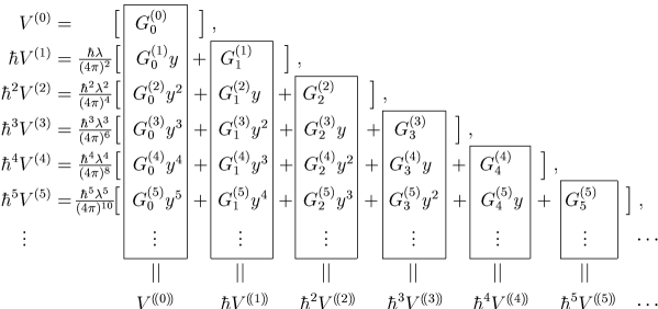
FIG. 1.: The loop expansion vs. the leading-logarithm expansion.