CBPF-NF-055/99 KL-TH 99/02 THES-TP 99/13 hep-th/9911177

Thermodynamics of the 2+1 dimensional Gross-Neveu model with complex chemical potential
H. R. Christiansen^†⋄, A. C. Petkou^⋆ , M. B. Silva Neto^†‡, N. D. Vlachos^⋆⋆
† Centro Brasileiro de Pesquisas Físicas, Rua Dr. Xavier Sigaud 150 - Urca,
CEP:22290-180, Rio de Janeiro, Brazil.

^⋆ Fachbereich Physik, Theoretische Physik, Universität Kaiserslautern
Postfach 3049, 67653 Kaiserslautern, Germany.

^‡ Instituto de Física, Universidade Federal do Rio de Janeiro,
Caixa Postal 68528, CEP:21945-970, Rio de Janeiro, Brazil.

^⋆⋆ Department of Theoretical Physics, Aristotle University of Thessaloniki,
Thessaloniki 54006, Greece.

^⋄ Group of Theoretical Physics, Universidade Católica de Petrópolis,
Rua Barão de Amazonas 124, Petrópolis 25685-070, Rio de Janeiro, Brazil.

Abstract:

We study the thermodynamics of the 2+1 dimensional Gross-Neveu model by introducing a representation for the canonical partition function which encodes both real and imaginary chemical potential cases. It is pointed out that the latter case probes the thermodynamics of possible anyon-like excitations in the spectrum. It is also intimately connected to the breaking of the discrete $Z$-symmetry of the model, which we interpret as signaling anyon deconfinement. Finally, the chiral properties of the model in the presence of an imaginary chemical potential are discussed and analytical results for the free-energy density at the transition points are presented.

1 Introduction

Chiral symmetry and its realization at finite temperature have been matter of intense studies for a long time. One of the most extensively used laboratories for this purpose has been the Gross-Neveu model [1] both at zero and finite temperature [2][3]. In the large-$N$ limit the $2+1$ dimensional version of this theory is renormalizable and provides a convenient arena for the survey of chiral symmetry; for instance, its dynamical breakdown at zero temperature and its high temperature restoration. Recently, there has been also considerable interest in studying the properties of chiral symmetry at finite density, or equivalently in the presence of a chemical potential [4, 5, 6]. This is believed to be relevant to the understanding of the physics of hot and dense matter which is expected to be probed in the laboratory by the RHIC experiments [7].

In this work, we address the thermodynamics and chiral properties of the 2+1 dimensional Gross-Neveu model in the canonical formalism. The use of the canonical formalism follows naturally when one introduces a constraint on the fermion number. Our discussion, however, will be based on a generalized representation of the canonical partition function that encodes the presence of a real chemical potential as a special case. It is shown that the approach yields similar results to the grand canonical formalism outcomes, the latter being the natural framework for studying systems in the presence of a chemical potential [8, 9]. This generalized partition function will also be studied for imaginary values of the chemical potential where it corresponds, rather surprisingly, to a real free-energy density.

We argue that the presence of an imaginary chemical potential is intimately connected to the possibility of having anyon-like excitations in the spectrum of the theory. We also show that the imaginary chemical potential emerges naturally in the 2+1 dimensional Gross-Neveu $U(1)$ gauged model at finite temperature. Such a theory has infinitely many $Z$-vacua [13] around which the gauge field may fluctuate. These fluctuations have been shown to be connected to peculiar excitations whose charge is not an integer multiple of the elementary charge of the theory. We interpret these excitations as being anyon-like [14] and argue that our generalized canonical partition function gives their free-energy density. As the gauge field fluctuations around the $Z$-vacua lead to the spontaneous breakdown of the discrete $Z$-symmetry, it appears that the latter is tied to an anyon confinement/deconfinement transition. Finally, we study the chiral properties of the Gross-Neveu model in the presence of an imaginary chemical potential. In this case the theory is chirally symmetric at high enough temperatures but it appears to be unstable at $T=0$. For any non-zero value of the imaginary chemical potential, chiral symmetry is broken at a certain temperature as the system cools down. This corresponds to a second-order phase transition where the free-energy density of the system is given by a remarkably simple analytic expression. There also exists a particular value of the temperature at which the system appears to be in a bosonic phase.

The paper is organized as follows. In Sec.2 we briefly review the 2+1 dimensional Gross-Neveu model at finite temperature. In Sec.3 we set the stage for studying the model with a constraint on the fermion number. Using a generalization of the well-known formula which gives the canonical partition function [10, 12, 11] we derive analytic expressions for the free-energy density, the fermion number density and the chiral order parameter. Our formalism coincides with the standard grand-canonical approach when the chemical potential takes real values. In Sec.4 we study the model in the presence of an imaginary chemical potential and show that it corresponds to a system possessing anyon-like excitations. We establish a connection with the breakdown of the $Z$-symmetry [13] of the $U(1)$ gauged Gross-Neveu model at finite temperature. In this way we give a physical interpretation to the canonical partition function with imaginary chemical potential as representing the free-energy needed to immerse an excitation of imaginary charge in the spectrum. We argue that such excitations are anyon-like. Next, we present results related to the properties of chiral symmetry in the presence of an imaginary chemical potential at finite temperature. In Sec.5 we summarize and discuss possible implications of our results.

2 The 2+1 dimensional Gross-Neveu model at finite temperature

The Euclidean Gross-Neveu model may be defined by the Lagrangian density [2, 15]

$${\cal L}=-\bar{\psi}^{i}\partial\!\!\!/\psi^{i}-\frac{g}{2}(\bar{\psi}^{i}\psi^{i})^{2},$$ (1)

where $\bar{\psi}^{i}$, $\psi^{i}$, $i=1,2,..,N$, are four-component Dirac fermions and $g$ is the coupling. In $d=3$ the massless model above is $U(2N)$-invariant and possesses a $Z_{2}$ discrete “chiral” symmetry

$$\psi\rightarrow\gamma_{5}\psi\,,\,\,\,\,\,\bar{\psi}\rightarrow-\gamma_{5}\bar{\psi}.$$ (2)

This model has been extensively used as a testing ground for studying the mechanism of chiral symmetry breaking in QCD [6].

For large-$N$, the model is studied in a $1/N$ expansion where it is renormalizable [15]. One introduces an auxiliary scalar field $\lambda(x)$ and integrates the fermions out. The partition function (generating functional) reads

$${\cal Z} = \int({\cal D}\lambda)e^{-NI_{eff}(\lambda,G)}\,,$$ (3)

$$I_{eff}(\lambda,G) = \frac{1}{2G}\int{\rm d}^{3}x{\;}\lambda^{2}(x)-Tr\left[\ln(\partial\!\!\!/+\lambda)\right]\,,$$ (4)

where the rescaled coupling $G=gN$ is kept finite as $N\rightarrow\infty$.

To leading order in $1/N$ the renormalized theory manifests itself in two different phases distinguished by a zero or a non-zero expectation value of $\langle\lambda\rangle$. This manifestation depends on the value of the renormalized coupling $1/G_{r}$ as compared to the critical coupling $1/G_{*}=4(2\pi)^{-3}\int{\rm d}^{3}p/p^{2}$. For $1/G_{r}>1/G_{*}$, $\langle\lambda\rangle=0$ and the theory is in a weakly-coupled phase where chiral symmetry is unbroken. For $1/G_{r}<1/G_{*}$, $\langle\lambda\rangle\neq 0$ and the theory is in a strongly-coupled phase where chiral symmetry is broken. In the latter case the fermions acquire a mass proportional to $\langle\lambda\rangle$. Clearly, $\langle\lambda\rangle$ plays the role of an order parameter for the chiral phase transition.

From the Euclidean formulation above one straightforwardly switches over to thermodynamics at temperature $T=1/\beta$ by making $x_{0}$ finite with length $L=1/T$ and imposing periodic (antiperiodic) boundary conditions over the interval $[0,L]$ for bosonic (fermionic) variables. In this way the bulk theory in 2+1 dimensions corresponds to a two-dimensional quantum system at zero temperature. It then follows that the $T=0$ system can be “prepared”, by appropriately tuning the coupling constant, to be either in the chirally symmetric or in the chirally broken phase. Had it been “prepared” to be in the broken (ordered) phase, one would expect that there exists a high temperature phase transition to the symmetric (disordered) phase. Such a transition is allowed (not forbidden) by the Mermin-Wagner-Coleman theorem as the relevant symmetry is discrete.

To study the chiral symmetry restoration one calculates the partition function (3) by the steepest descent method for large-$N$. This amounts to performing a $1/N$ expansion for ${\cal Z}$ around its saddle-points, which correspond to uniform values of $\langle\lambda\rangle$. The latter are obtained from the gap equation

$$\frac{1}{G}=\frac{4}{L}\sum_{n=-\infty}^{\infty}\int\frac{{\rm d}^{2}{\bf p}}{(2\pi)^{2}}\frac{1}{{\bf p}^{2}+\omega_{n}^{2}+\langle\lambda\rangle^{2}}\,,\,\,\,\,\,\omega_{n}=(2n+1)\frac{\pi}{L}\,,n=0,\pm 1,\pm 2,\dots\,.$$ (5)

This expression is divergent but all UV divergences at finite temperature are the same as at zero temperature [15]. Therefore, one can renormalize (5) by substituting for $1/G$ its corresponding renormalized value at $T=0$. For the system to be in the chirally broken phase at $T=0$ one sets

$$\frac{1}{G}\rightarrow\frac{1}{G_{r}}=-\frac{m}{\pi},$$ (6)

where $m>0$ is the dynamically induced mass of the elementary fermions at $T=0$. Then, from (5) one obtains

$$\langle\lambda\rangle=\frac{2}{L}\ln{\left[\frac{e^{Lm/2}+\sqrt{e^{Lm}-4}}{2}\right]}\,,$$ (7)

which gives the dependence of the order parameter $\langle\lambda\rangle$ on the temperature. In particular, $\langle\lambda\rangle$ vanishes at the second-order phase transition point $1/L_{c}=T_{c}=m/2\ln{2}$ where chiral symmetry is restored. At this point and for higher temperatures, the free-energy density is given to leading-$N$ by

$$\frac{f}{N}=-\frac{3\zeta(3)}{2\pi L^{3}}\,,$$ (8)

and coincides with the free-energy density of $2N$ massless four-component Dirac fermions [19].

3 Thermodynamics of the 2+1 dimensional Gross-Neveu model in the canonical formalism

3.1 General Setting

The canonical formalism for the analysis of the thermodynamics of a system has been recently employed in studies of fermionic systems at finite baryon density [11, 12]. The reason is that it bypasses the usual sign problem of the Euclidean fermion determinant for real values of the chemical potential. Since the three-dimensional Gross-Neveu model does not undergo this sign problem, it has been extensively studied in the standard grand-canonical formalism both analytically and numerically [4, 5]. Nevertheless, it would still be interesting to perform a direct analysis in the canonical formalism in order to test results obtained previously. Furthermore, in doing so, we obtain some surprising new results which shed new light into the thermodynamics of the model.

The canonical partition function can be obtained as the thermal average over eigenstates of the number operator $\hat{N}=\int{\rm d}^{2}{\it{\bf x}}{\;}\psi^{\dagger}(\tau,{\bf x})\psi(\tau,{\bf x})$ with fixed eigenvalues $B$. Namely, [8]

$${\cal Z}(T,V,B)=Tr\left(e^{-\beta\hat{H}}\delta(\hat{N}-B)\right),$$ (9)

where $\hat{H}$ is the Hermitian Hamiltonian. As usual, ${\hat{N}}$ measures the excess of fermions over anti-fermions in the spectrum.

If one anticipates that for certain physical conditions the spectrum contains free fermions or anti-fermions, then $B$ must be an integer. This then leads to the following representation for the canonical partition function [10]

$${\cal Z}(T,V,B)=\frac{1}{2\pi}\int_{0}^{2\pi}{\rm d}\phi\,e^{-{\rm i}\phi B}{\cal Z}(T,V,i\phi)\,,$$ (10)

where, ${\cal Z}(T,V,{\rm i}\phi)$ is the grand-canonical counterpart with imaginary chemical potential. If on the other hand one is interested in physical situations where $B$ is the mean fermion (anti-fermion) density, then $B$ is real, not necessarily integer, and (10) is no more a valid representation.

In this work we propose a generalization of Eq.(10) which is suitable for both analytic and numerical work. Our representation includes both cases of integer and non-integer real values of $B$. Furthermore, it leads to some unexpected new results when $B$ is imaginary. Our representation follows from Eq.(9) if we write the delta-function constraint with the help of an auxiliary Lagrange multiplier scalar field $\theta(\tau)$ as

$${\cal Z}(T,V,B) = \int({\cal D}\lambda)({\cal D}\theta)e^{-N{\cal I}_{eff}(\lambda,g;\theta,B)}$$ (11)

$$= e^{-\beta F(T,V,B)},$$

which enforces the averaged fermion number constraint $\langle\hat{N}\rangle=B$. Here, $F(T,V,B)$ is the free-energy and ${\cal I}_{eff}$ is the following effective action

$${\cal I}_{eff}(\lambda,g;\theta,B)={\rm i}\frac{B}{N}\int_{0}^{L}{\rm d}\tau{\;}\theta(\tau)+\frac{1}{2G}\int_{0}^{L}{\rm d}\tau\int{\rm d}^{2}{\bf x}{\;}\lambda^{2}(\tau,{\bf x})-Tr[\ln(/\!\!\!\partial+\lambda(\tau,{\bf x})+{\rm i}\gamma_{0}\theta(\tau))]_{L}\,.$$ (12)

To evaluate the free-energy in (11) for large-$N$, we expand $I_{eff}$ around its stationary points assuming constant (translation invariant) $\langle\lambda\rangle$ and $\langle\theta\rangle$ configurations. These satisfy the following set of saddle-point equations

$$\frac{1}{G} = \frac{4}{L}\sum_{n=-\infty}^{\infty}\int\frac{{\rm d}^{2}{\bf p}}{(2\pi)^{2}}\frac{1}{{\bf p}^{2}+(\omega_{n}+\langle\theta\rangle)^{2}+\langle\lambda\rangle^{2}},$$ (13)

$${\rm i}\frac{B}{N} = \lim_{\rho\rightarrow 0}\frac{4}{L}\int\frac{{\rm d}^{2}{\bf p}}{(2\pi)^{2}}\sum_{n=-\infty}^{\infty}\frac{e^{{\rm i}\omega_{n}\rho}(\omega_{n}+\langle\theta\rangle)}{{\bf p}^{2}+(\omega_{n}+\langle\theta\rangle)^{2}+\langle\lambda\rangle^{2}},$$ (14)

where $\omega_{n}=(2n+1)\pi/L$, $n=0,\pm 1,\pm 2,..$. [20, 19]. We can subtract the UV divergences in Eq.(13) [19] by adjusting the renormalized coupling as in (6). At the same time the system at $T=0$ can be arranged so as to break chiral symmetry. After some algebra we obtain

$$0 = \langle\lambda\rangle-m+\frac{1}{L}\left[\ln\left(1+e^{-L\langle\lambda\rangle-{\rm i}L\langle\theta\rangle}\right)+\ln\left(1+e^{-L\langle\lambda\rangle+{\rm i}L\langle\theta\rangle}\right)\right],$$ (15)

$$\frac{\tilde{B}}{N} = \frac{\langle\lambda\rangle}{2\pi L}\left[\ln\left(\frac{1+e^{-L\langle\lambda\rangle+{\rm i}L\langle\theta\rangle}}{1+e^{-L\langle\lambda\rangle-{\rm i}L\langle\theta\rangle}}\right)-Li_{2}\left(-e^{-L\langle\lambda\rangle+{\rm i}L\langle\theta\rangle}\right)+Li_{2}\left(-e^{-L\langle\lambda\rangle-{\rm i}L\langle\theta\rangle}\right)\right],$$ (16)

where $\tilde{B}=B/V$ is the fermion density. From (11) and (12) we can now calculate the renormalized free-energy density $f=F/V$ to leading-$N$ and obtain

$$\frac{1}{N}f(\beta,m;\langle\lambda\rangle,\tilde{B}) = \frac{\langle\lambda\rangle^{3}}{3\pi}-\frac{m\langle\lambda\rangle^{2}}{2\pi}+2{\rm i}\tilde{B}\langle\theta\rangle+\frac{1}{6\pi L^{3}}\left[Li_{3}(-e^{-L\langle\lambda\rangle+{\rm i}L\langle\theta\rangle})+Li_{3}(-e^{-L\langle\lambda\rangle-{\rm i}L\langle\theta\rangle})\right.$$ (17)

$$\left.-\ln(e^{-L\langle\lambda\rangle})\left(Li_{2}(-e^{-L\langle\lambda\rangle+{\rm i}L\langle\theta\rangle})+Li_{2}(-e^{-L\langle\lambda\rangle-{\rm i}L\langle\theta\rangle})\right)\right].$$

The functions $Li_{n}(z)$ are the standard polylogarithms [21].

In principle, the free-energy density (17) together with the gap equations (15) and (16) are sufficient for studying the thermodynamic properties of the Gross-Neveu model to leading-$N$. Before we proceed, however, we observe that requiring the free-energy density in (17) to be real we are naturally led to distinguish two cases. Namely, as the terms involving polylogarithms in (17) are real for both real and imaginary values of $\langle\theta\rangle$, we can have either 1) $\langle\theta\rangle$=imaginary and $\tilde{B}$=real, or 2) $\langle\theta\rangle$=real and $\tilde{B}$=imaginary. Clearly, ${\bf 1)}$ would correspond to the usual case of the Gross-Neveu model with real chemical potential. Nevertheless, we will show that case ${\bf 2)}$ probes some interesting properties of the Gross-Neveu model too.

3.2 Relation to the grand-canonical formalism

For $\langle\theta\rangle$=imaginary (17) is the free-energy density of the Gross-Neveu model with ordinary (real) chemical potential. Indeed, setting ${\rm i}\langle\theta\rangle=\mu<m$ we find that (15) and (16) coincide with the corresponding expressions for the gap equation and the fermion density, the latter was obtained for the first time in [5]. Namely,

$$\langle\lambda\rangle = \frac{1}{L}\ln\left[\frac{e^{Lm}-2\cosh(L\mu)+\sqrt{(e^{Lm}-2\cosh(L\mu))^{2}-4}}{2}\right],$$ (18)

$$\frac{\tilde{B}}{N} = \frac{\langle\lambda\rangle}{2\pi L}\left[\ln\left(\frac{1+e^{-L\langle\lambda\rangle+L\mu}}{1+e^{-L\langle\lambda\rangle-L\mu}}\right)-Li_{2}\left(-e^{-L\langle\lambda\rangle+L\mu}\right)+Li_{2}\left(-e^{-L\langle\lambda\rangle-L\mu}\right)\right]\,.$$ (19)

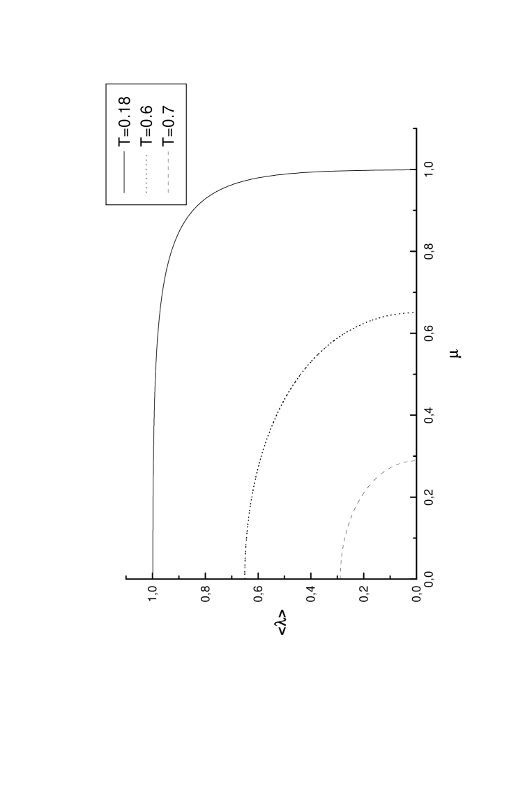
Figure 1: Critical lines in the $\langle\lambda\rangle-\mu$ plane for various $T<T_{c}$. For simplicity we chose $m=1$ such that $T_{c}\approx 0.72$.

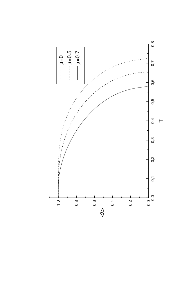
Figure 2: $\langle\lambda\rangle$ vs $T$ for various $\mu$, when $m=1$.

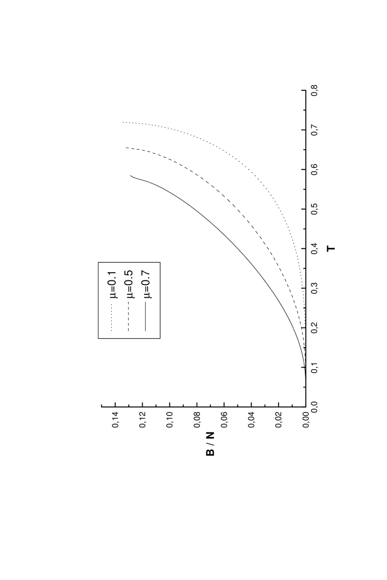
Figure 3: $\tilde{B}/N$ vs $T$ for various $\mu$ and $m=1$. The baryon density blows up at $T\rightarrow T_{c}(\mu)$.

The thermodynamic properties here are well-known. As the chemical potential $\mu$ increases from zero, the critical temperature $T_{c}$ for the chiral symmetry restoration decreases. This critical temperature becomes zero at some critical value of the chemical potential $\mu_{c}\equiv m$ where the chiral symmetry restoration is of first order. One can draw a physical picture of the chiral symmetry restoration in terms of overlapping composites. When the temperature is increased, chiral condensates begin to overlap as their radius grow up. At some critical point the system is mainly composed of overlapping condensates which, as a result, are no longer the good basis for describing the thermodynamic properties of the system and the fermionic constituents must be taken into account. It is then reasonable to expect that by increasing the baryon density, which amounts to increasing the density of chiral condensates, a lower critical temperature would be needed for the system to reach the critical point above. In Fig.1 we plot the critical lines in the $\langle\lambda\rangle$-$\mu$ plane for various values of $T$. In Fig.2 we plot $\langle\lambda\rangle$ vs $T$ for various values of $\mu$. In Fig. 3 we plot the fermion density $\tilde{B}/N$ vs $T$ for various values of $\mu$. For $\mu>0$ the fermion density is discontinuous at a critical temperature $T_{c}(\mu)$.

4 Imaginary chemical potential

4.1 The connection with an anyon-like system (anyon confinement/deconfinement)

Consider the interaction of the Gross-Neveu model (1) with an external $U(1)$ gauge potential $A_{\mu}(x)$. The Euclidean Lagrangian density reads

$${\cal L}=-\bar{\psi^{i}}(/\!\!\!\partial-{\rm i}e/\!\!\!\!A)\psi^{i}-\frac{g}{2}(\bar{\psi^{i}}\psi^{i})^{2},$$ (20)

where $e$ is the electric charge. Let us consider a constant potential $A_{0}\equiv\theta$ along the “time” direction. We can imagine embedding the model above into a 4-dimensional space. Due to the finite length of the $x_{0}$ dimension and the antiperiodic boundary conditions of the fermions along it, the system may be viewed as existing in a 3-dimensional hyper-cylinder whose axis is the 4^th (unobservable) dimension. The constant potential $A_{0}$ may now be regarded as the “vector” potential generated by a thin solenoid of magnetic flux $\Phi=\theta L$ along the axis of the hyper-cylinder. Such a picture corresponds to fermions encircling a thin solenoidal magnetic flux and one might expect to encounter Aharonov-Bohm type phenomena [14].

The potential in (20) may be gauged away by the transformation

$$\psi\rightarrow e^{{\rm i}e\theta\tau}\psi\,\,.$$ (21)

Such a transformation, however, “twists” the antiperiodic boundary conditions for the fermions unless

$$\theta=\frac{2\pi}{eL}k\,,\,\,\,\,\,k=0\pm 1,\pm 2,\dots\,\,.$$ (22)

The configurations with “twisted” boundary conditions may be viewed as anyon-like excitations [14]. For instance, the “quasi-particle” propagator of the above model (20)

$$S(x_{0},{\bf x};A_{0},\langle\lambda\rangle)=(/\!\!\!\partial+{\rm i}e\gamma_{0}A_{0}+\langle\lambda\rangle)S_{0}(x_{0},{\bf x};A_{0},\langle\lambda\rangle)\,,$$ (23)

has the following representation as a sum over non-trivial topological paths

$$S_{0}(x_{0},{\bf x};A_{0},\langle\lambda\rangle)=\sum_{l=-\infty}^{\infty}e^{{\rm i}\pi l}\,e^{{\rm i}(lL+x_{0})eA_{0}}\Pi(x_{0}+lL,{\bf x};\langle\lambda\rangle)\,,$$ (24)

where $\Pi(x_{0},\bf{x};\langle\lambda\rangle)$ are free boson propagators of mass $\langle\lambda\rangle$. Furthermore, since in our generalized representation of the partition function (11) we imposed a constraint on the average fermion number, we can have local charge density fluctuations $b(\tau,{\bf x})$ which give rise to the so-called statistical gauge field $a_{\mu}(\tau,{\bf x})$ as

$$b(\tau,{\bf x})=\psi^{\dagger}(\tau,{\bf x})\psi(\tau,{\bf x})-\tilde{B}=\partial_{1}a_{2}(\tau,{\bf x})-\partial_{2}a_{1}(\tau,{\bf x})=\epsilon^{0ij}\partial_{i}a_{j}(\tau,{\bf x})\,.$$ (25)

This (non-dynamical) field would be responsible for the anyon dynamics [22]. Finally, the partition function of the free theory i.e (20) at $g=0$, has been shown to reproduce the standard anyon virial coefficients [23].

The existence of the anyonic excitations above may be tied to a discrete $Z$-symmetry of the 2+1 dimensional Gross-Neveu model interacting with a standard $U(1)$ gauge field $A_{\mu}(x)$ at temperature $T$. The partition function in this case is

$${\cal Z}=\int({\cal D}A_{\mu})({\cal D}\psi)({\cal D}\bar{\psi})e^{-\int_{T}\left[\frac{1}{4}F_{\mu\nu}F_{\mu\nu}-\bar{\psi}^{i}(/\!\!\!\partial-{\rm i}e/\!\!\!\!A)\psi^{i}-\frac{g}{2}(\bar{\psi}^{i}\psi^{i})^{2}\right]},$$ (26)

where $F_{\mu\nu}=\partial_{[\mu}A_{\nu]}$ as usual. This theory is invariant under

$$A_{\mu}(\tau,{\bf x}) \rightarrow A_{\mu}(\tau,{\bf x})+\partial_{\mu}\chi(\tau,{\bf x})\,,$$ (27)

$$\psi(\tau,{\bf x}) \rightarrow e^{{\rm i}e\chi(\tau,{\bf x})}\psi(\tau,{\bf x})\,,$$ (28)

$$\bar{\psi}(\tau,{\bf x}) \rightarrow \bar{\psi}(\tau,{\bf x})e^{-{\rm i}e\chi(\tau,{\bf x})}\,,$$ (29)

which are the usual small gauge transformations provided they are periodic in Euclidean time $\tau$

$$\chi(0,{\bf x})=\chi(L,{\bf x})\,\,\,\mbox{and}\,\,\,\partial_{\mu}\chi(0,{\bf x})=\partial_{\mu}\chi(L,{\bf x})\,.$$ (30)

In addition to these, the theory is also invariant under large gauge transformations which are given by

$$\chi(0,{\bf x})=\chi(L,{\bf x})+\frac{2\pi}{e}k\,,\,\,\,\,\,k=\pm 1,\pm 2,\dots.$$ (31)

and represent a global $Z$-symmetry. This symmetry implies the existence of infinitely many equivalent $Z$-vacua in the theory (26). Namely, the gauge field configurations

$$A_{\mu}^{Z}(\tau,{\bf x})=(\frac{2\pi}{eL}k,0,0),\,\,\,k=0,\pm 1,\pm 2,\dots,$$ (32)

are lowest energy and equivalent since they are connected by gauge transformations of the form $\chi(\tau,{{\bf x}})=(2\pi/eL)\tau$. Still, such $Z$-transformations preserve the anti-periodic boundary conditions. We therefore conclude that Eq.(32) represents equivalent vacuum configurations of (26).

Going back to (20) provided condition (22) holds, the theory can be interpreted as a Gross-Neveu model with a $U(1)$ gauge coupling at finite temperature and lying in one of the $Z$-vacua. In this case there exist no anyon-like excitations in the spectrum. If condition (22) is relaxed, then (20) corresponds to the gauge theory above where the gauge field fluctuates around the $Z$-vacua. In the latter case there exist anyon-like excitations in the spectrum.

We can now construct an order parameter to distinguish the two cases as follows. Consider translational invariant fluctuations around the $Z$-vacua in (26) such that

$$A_{\mu}=A_{\mu}^{Z}+\theta(\tau)\,,\,\,\,\,\,\theta(0)=\theta(L).$$ (33)

Take now the quantity

$$\langle{\cal P}_{\tilde{e}}\rangle=\langle e^{{\rm i}\tilde{e}\int_{0}^{L}{\rm d}\tau\,\theta(\tau)}\rangle,$$ (34)

where $\tilde{e}/e\neq$ integer and the average is taken with respect to the partition function (26). It is not difficult to see that (34) is invariant under the strictly periodic gauge transformations (30). It is not invariant, however, under the $Z$-transformations (31). To see this consider the transformations

$$\theta(\tau)\rightarrow\theta(\tau)+\frac{2\pi}{eL}k\,,\,\,\,k=\pm 1,\pm 2,\dots,$$ (35)

which are symmetries of the theory (26) provided there is $Z$-invariance. Under (35)

$$\langle{\cal P}_{\tilde{e}}\rangle\rightarrow e^{{\rm i}2\pi k\frac{\tilde{e}}{e}}\langle{\cal P}_{\tilde{e}}\rangle\neq\langle{\cal P}_{\tilde{e}}\rangle.$$ (36)

The physical interpretation of (34) is that $F_{\tilde{e}}=-(1/\beta)\ln\langle{\cal P}_{\tilde{e}}\rangle$ gives the free-energy necessary to immerse a configuration of charge $\tilde{e}$ in the spectrum of the system [3]. If the theory (26) is in a $Z$-vacuum, then the spectrum can contain only an integer number of fermions or antifermions since, as explained earlier, it does not contain anyon-like excitations. In this case one clearly expects that $F_{\tilde{e}}=\infty$ or $\langle{\cal P}_{\tilde{e}}\rangle=0$. If on the other hand the theory is not in a $Z$-vacuum, then there exist anyon-like configurations in the spectrum and one in general expects that $\langle{\cal P}_{\tilde{e}}\rangle\neq 0$. We conclude that, in this sense, the $Z$-symmetry of the full gauge theory (26) is connected to the “confinement” or “screening” of anyons, where $\langle{\cal P}_{\tilde{e}}\rangle$ is the relevant order parameter. The anyonic theory preserves $Z$-symmetry in the confined phase where $\langle{\cal P}_{\tilde{e}}\rangle=0$ and violates the $Z$-symmetry in the deconfined phase where $\langle{\cal P}_{\tilde{e}}\rangle\neq 0$.

We are now in a position to give a physical interpretation to the partition function (11) with real $\langle\theta\rangle$ (imaginary chemical potential), as a result of the following identity

$${\cal Z}(T,V,B)=e^{-\beta F(T,V,B)}\equiv\langle{\cal P}_{\tilde{B}/N}\rangle\,.$$ (37)

Namely, the free-energy of the Gross-Neveu model with imaginary chemical potential represents the free-energy of anyon-like configurations emerging in the spectrum when the model is coupled to a $U(1)$ gauge field which fluctuates around the $Z$-vacua.

The above discussion concerning the order parameter (34) parallels the discussion in [13] of a similar order parameter for the confinement or screening of incommensurate charges in parity invariant QED₃ (see also [24]). One of the new observations here is the interpretation of the incommensurate charged configurations as being anyon-like. Another important point is that the order parameter $\langle{\cal P}_{\tilde{e}}\rangle$ is in fact imaginary for any real value of $\tilde{e}$. This is also seen from (17) or (37). If (34) is to be interpreted as a physical free-energy density, it is necessary that $\tilde{e}$ is imaginary. The fact that we obtain an imaginary eigenvalue $B=\tilde{e}$ for the Hermitian operator $\hat{N}$ means essentially that we are not using a positive definite density matrix to describe the fluctuations around the $Z$-vacua of the theory (26). Nevertheless, even in that case we will be able to extract useful results for the critical properties of the theory, assuming that the latter are universal.

4.2 Chiral Symmetry and $Z$-vacua

The chiral symmetry restoration for real $\langle\theta\rangle$ can be inferred from the gap equation (15). The critical line separating the chirally symmetric from the chirally broken phase in the $\langle\theta\rangle$-$T$ plane is obtained by setting $\langle\lambda\rangle=0$ in (15) as

$$\langle\theta\rangle=\frac{1}{L}\arccos\left[\frac{e^{Lm}}{2}-1\right],$$ (38)

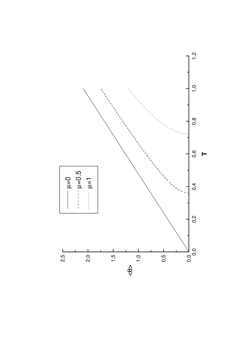
Figure 4: Critical lines in the $\langle\theta\rangle-T$ plane for various $m$ when $\langle\theta\rangle/T\in[0,\pi]$. The line $\langle\theta\rangle=(2\pi/3)T$ is an asymptote.

and is depicted for various values of $m$ in Fig.4 when $\langle\theta\rangle/T\in[0,\pi]$.

In order to discuss the chiral properties of the theory we shall henceforth consider, for concreteness, the massless case where the system is critical already at $T=0$. In this case, when the chemical potential is real one does not expect any phase transition as the temperature rises up. To put it differently and in a more general ground, for real chemical potential the system is chirally symmetric at some high temperature and as it cools down chiral symmetry is, in general, broken at some lower critical temperature. Having chosen $m=0$ this critical temperature is $T=0$. Consider now the case when $\langle\theta\rangle$ is real, where this corresponds to an imaginary chemical potential or some fluctuation around the $Z$-vacua as explained above. Again, at high enough temperatures we expect the system to be chirally symmetric. However, chiral symmetry is now broken at a non-zero temperature $T=3\langle\theta\rangle/2\pi$. The important point is that as the system cools down, chiral symmetry remains broken in a “temperature window” $3\langle\theta\rangle/2\pi\geq T\geq 3\langle\theta\rangle/4\pi$ and then it is restored again. Furthermore, as $T\rightarrow 0$, it passes through infinitely many “windows” of the form

$$\frac{3\langle\theta\rangle}{2\pi}\frac{1}{1+3k}\geq T\geq\frac{3\langle\theta\rangle}{2\pi}\frac{1}{2+3k}\,,\,\,\,k=0,1,2,\dots,$$ (39)

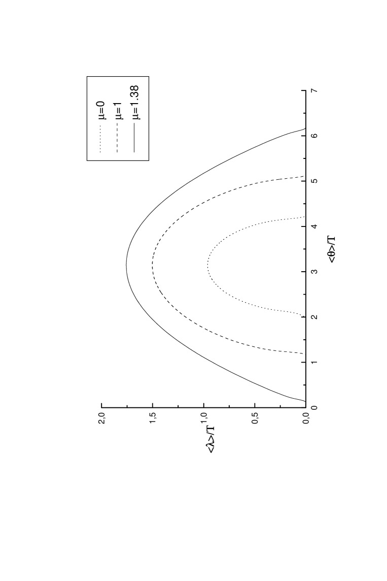
Figure 5: $\langle\lambda\rangle/T$ vs $\langle\theta\rangle/T$ for $0<m/T<2\ln 2$. For fixed, non-zero $\langle\theta\rangle$, $T$ decreases along the horizontal axis as one moves to the right.

in which chiral symmetry is always broken. This essentially means that for any real non-zero $\langle\theta\rangle$ the $T=0$ theory becomes unstable. The relevant physical picture can be read off from Fig.5 where we plot $\langle\lambda\rangle/T$ vs $\langle\theta\rangle/T$ in $0\leq m/T\leq 2\ln 2$. Note that for $m/T>2\ln 2$ the theory is always in a chirally broken phase.

We can draw a physical picture for the chiral symmetry restoration discussed above. The magnetic flux (25) associated with local charge fluctuations catalyzes symmetry breaking as it stabilizes the chiral condensates against thermal fluctuations inside the “temperature windows” (39) . The fact that in the high-temperature weakly coupled regime even a small imaginary chemical potential induces chiral symmetry breaking, shows that the former plays the role of a strong catalyst of dynamical symmetry breaking, similar to that of a transverse external magnetic field [25] or a constant negative curvature [26]. The chiral symmetry restoration transition at $T=3\langle\theta\rangle/2\pi$ is of the second-order with mean field critical exponents [14, 20] since the order parameter $\langle\lambda\rangle$ is continuous. The order parameter acquires its maximum value for $T=\langle\theta\rangle/\pi$ and then starts to drop until it reaches zero again at $T=3\langle\theta\rangle/4\pi$. The same picture holds for all chiral restoration “temperature windows” (39).

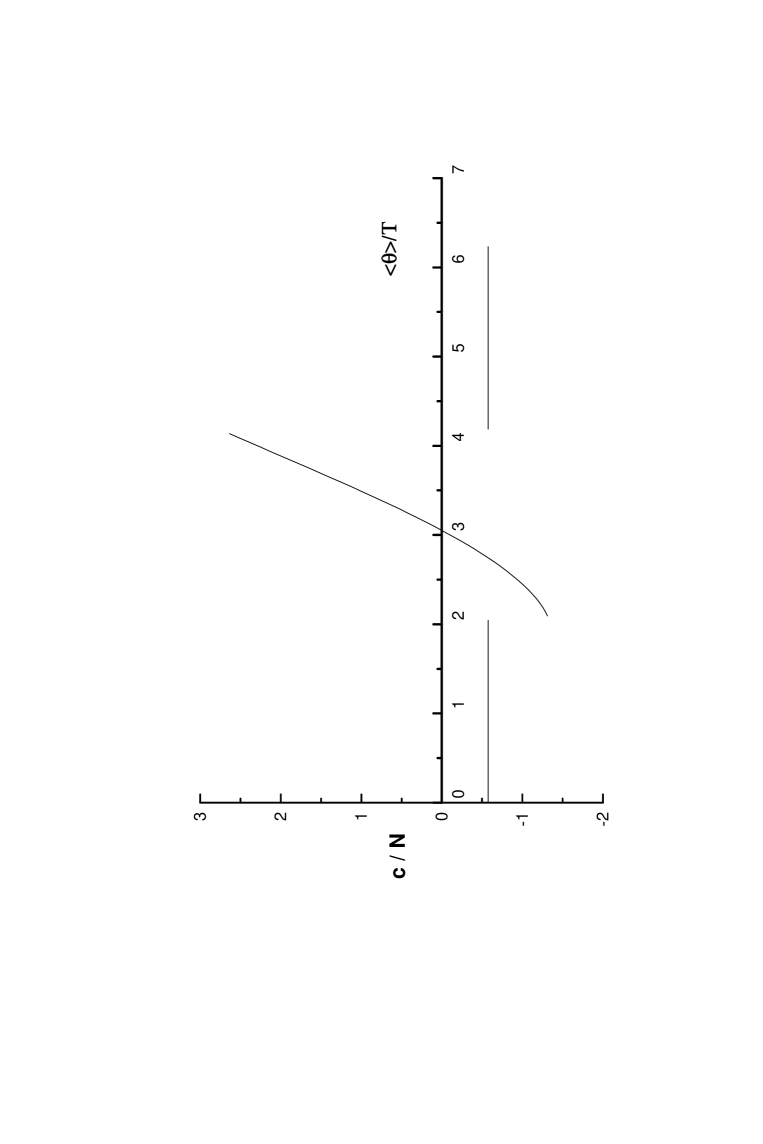
Figure 6: The free-energy density vs $\langle\theta\rangle/T$. As in Fig.5, $T$ decreases along the horizontal axis as one moves to the right.

It is also interesting to study the behavior of the free-energy density as a function of the temperature for non-zero $\langle\theta\rangle$. This is depicted in Fig.6 where we plot the free-energy density vs $\langle\theta\rangle/T$. For high enough $T$ the system is in the chirally symmetric phase and to leading-$N$ the free-energy density equals that of $N$ massless free four-component Dirac fermions e.g. Eq.(8). At $T=3\langle\theta\rangle/2\pi$ the free-energy jumps discontinuously to a local minimum and then raises until it reaches a local (positive) maximum at $T=3\langle\theta\rangle/4\pi$ where it drops again discontinuously to the value (8). Similar fluctuations occur for all the infinitely many temperature “windows” (39) as $T\rightarrow 0$.

It is rather intriguing that we are able to give analytic expressions for the free-energy density of the system at the end-points of the “temperature windows” of chiral symmetry breaking, $3\langle\theta\rangle/2\pi$, $3\langle\theta\rangle/4\pi$ (in fact this is possible for the end-point of all the “windows” (39)). After some algebra we obtain respectively

$$\frac{f_{L}}{N} = -\frac{1}{\pi L^{3}}\left[\frac{4\pi}{3}Cl_{2}\left(\frac{\pi}{3}\right)-\frac{2}{3}\zeta(3)\right]\,,$$ (40)

$$\frac{f_{L}}{N} = \frac{1}{\pi L^{3}}\left[\frac{8\pi}{3}Cl_{2}\left(\frac{\pi}{3}\right)+\frac{2}{3}\zeta(3)\right]\,,$$ (41)

where, $Cl_{2}(\phi)={\rm Im}[Li_{2}(e^{{\rm i}\phi})]$ is the Clausen function [21]. Note that $Cl_{2}(\pi/3)$ is the absolute maximum of this function which is a well-documented irrational number [28].

The results for the free-energy density have been on purpose written as above, in order to be compared with the expected scaling form of the free-energy density of a conformal field theory (CFT). The point is that the chiral phase transition in the 2+1 dimensional model above is of second-order and one would expect it to correspond to the universality class of a 3-dimensional CFT. When a CFT is put in a finite-size geometry (i.e. in a slab with one finite dimension of length $L$), its free-energy density scales as [18]

$$f_{L}=-\frac{\tilde{c}\,\zeta(3)}{2\pi L^{3}}\,\cdot$$ (42)

The quantity $\tilde{c}$ coincides with the central charge in $d=2$ and has been recently proposed [29] to be a possible generalization of a $Cl$-function in $d>2$. Clearly, from (40), (41) and (42) we see that the chiral transition above appears to be connected to new 3-dimensional CFTs. The fact that $\tilde{c}$ in (40) is less than the corresponding free-field theory value (8) and it is negative in (41), seems to imply that the above critical theories may not be unitary. Nevertheless, such theories may conceivably correspond to three-dimensional versions of the non-unitary two-dimensional Lee-Yang model [32].

The middle point of the chiral transition “temperature window” (39) is also interesting. At this point $\langle\lambda\rangle$ takes its maximal value. From (15) we obtain for $\langle\theta\rangle=\pi/L$,

$$\langle\lambda\rangle=\frac{2}{L}\ln\left(\frac{1+\sqrt{5}}{2}\right).$$ (43)

This value equals the value one obtains for the mass of the elementary bosonic modes in the 2+1 dimensional $O(N)$ vector model at finite temperature, when the theory is critical at $T=0$ [30]. Plugging this into (17) we can calculate the free-energy density which, by virtue of some non-trivial polylogarithmic identities [30, 31] is found to be

$$\frac{f_{L}}{N}=\frac{16}{5}\frac{\zeta(3)}{2\pi L^{3}}.$$ (44)

This is exactly minus the free-energy density of the 2+1 dimensional $O(4N)$ vector model at its non-trivial critical point. In principle, a positive free-energy density which would correspond to negative pressure and negative entropy seems to be a rather unphysical result [33]. However, one might try to construct a physical system where the result (44) could make sense. This is the $O(4N)$ ${\cal N}=1$ supersymmetric sigma model [34, 35] in the presence of an external $A_{0}$ potential at finite temperature. To leading-$N$, the free-energy density of this theory is simply given by the sum of the free-energies of fermions and bosons. In general, supersymmetry is expected to be broken at any finite temperature [36]. Nevertheless, it may happen that for some temperature the fermion contribution, given by (44), and the boson contribution cancel each other and the system becomes supersymmetric again. Note that the matching of the bosonic and fermionic degrees of freedom is correct - the ${\cal N}=1$ supermultiplet in three-dimensions requires $2N$ two-component Majorana fermions. A similar bosonization of fermions has been recently discussed in [37].

5 Summary and Discussion

In this work we studied the 2+1 dimensional Gross-Neveu model in the presence of an imaginary chemical potential and argued that it provides an interesting ground for probing the properties of chiral symmetry at non-zero temperature. In Sec.3 we proposed a generalization of the well-known formula for the canonical partition function and presented analytic expressions for the free-energy density, the fermion number density and the chiral order parameter $\langle\lambda\rangle$. We demonstrated that this general formalism includes the standard grand-canonical formalism when the chemical potential is real. In Sec.4 we focused on the case of imaginary chemical potential. We considered a $U(1)$ gauge field coupled to the Gross-Neveu model at finite temperature. Such a theory possesses infinitely many equivalent $Z$-vacua. We showed that when the gauge field fluctuates around these Z-vacua, as given by Eq.(33), anyon-like excitations manifest themselves in the spectrum of the 2+1 dimensional Gross-Neveu model. This is established by showing that the free-energy necessary to immerse such an excitation is non-zero. Furthermore, we provided evidence that the expectation value of the abelian Polyakov loop, which is the order parameter for establishing whether the above $U(1)$ gauge theory resides in one of the $Z$-vacua, coincides with the canonical partition function for imaginary values of the fermion number density. This way we gave a physical interpretation to the canonical partition function with imaginary chemical potential as being the free-energy needed to immerse an excitation of imaginary charge in the spectrum of the 2+1 dimensional Gross-Neveu model. The latter excitation is related to the anyon-like excitations discussed above. Finally, we gave some results connected to the properties of chiral symmetry in the presence of an imaginary chemical potential at finite temperature.

Studies of the critical thermodynamic properties of a system undergoing a phase transition are intimately connected to the Lee-Yang zeroes [38, 39]. These are the zeroes of the partition function for imaginary values of the external magnetic field, the latter being the “conjugate” variable of the relevant order parameter. It is then conceivable that one could try to investigate the critical properties of a system at finite density by studying its partition function (or its free-energy density), at complex values of the number density, the latter being the “conjugate” variable of the chemical potential. In this sense, the results presented in this work are closely related to a Lee-Yang zeroes analysis.

These results can be extended in several directions. For example,it is possible in principle to study numerically the partition function (11) for complex chemical potential and establish the chiral symmetry restoration “windows” advocated above. It is also possible to numerically compute the free-energy densities at the critical points and compare them with our analytic results (40) and (41). Furthermore, it would be interesting to compare the free energy density (17) to the one recently proposed by Laughlin [40] in order to reproduce the anomalous behaviour of the thermal conductivity in some high-temperature superconductors of the BSCCO family [41] . Since these compounds exhibit a new kind of phase transition induced by strong catalysts of dynamical symmetry breaking, it is plausible that our generalized canonical partition function formalism can be used to explain such unusual behavior. Finally, based on the results of the present work, it may be interesting to explore the possibility of finite temperature supersymmetry restoration in ${\cal N}=1$ supersymmetric theories [43].

Acknowledgements

The work of H.R.C. and M.B.S.N was supported in part by the Brazilian agencies for the development of science FAPERJ and CAPES. A.C.P was supported in part by an I.K.Y. Postdoctoral Fellowship and an Alexander von Humboldt Fellowship. N.D.V. was supported by the E.U. under TMR contract No. ERBFMRX–CT96–0090.

References

- [1] D. Gross and A. Neveu, Phys. Rev. D10, 3235 (1974).
- [2] B. Rosenstein, B. J. Warr and S. H. Park, Phys. Rep. 205, 59 (1991).
- [3] D. Gross, R. D. Pisarski and L. G. Yaffe, Rev. Mod. Phys. 53, 43 (1981).
- [4] S. Hands, Nucl. Phys. A642, 228 (1998); hep-lat/9806022.
- [5] S. Hands, A. Kocić and J. B. Kogut, Nucl. Phys. B390, 355 (1993); hep-lat/9208022.
- [6] K. Strouthos and J. B. Kogut, Chiral Symmatry Restoration in the Three-Dimensional Four Fermion Model at Nonzero Temperature and Density, hep-lat/9904008.
- [7] F. Wilczek, The Recent Excitement in High Temperature QCD, hep-ph/9908480.
- [8] J. I. Kapusta, Finite Temperature Field Theory, Cambridge Monographs on Mathematical Physics, 1989.
- [9] R. Hagedorn and K. Redlich, Z. Phys. C27, 541 (1985).
-
[10]
N. Weiss, Phys. Rev. D35, 2495 (1987);
A. Roberge and N. Weiss, Nucl. Phys. B275, 734 (1986). - [11] M. Alford, A. Kapustin and F. Wilzcek, Phys. Rev. D59, 054502 (1999); hep-lat/9807039.
- [12] F. Karsch, Lattice QCD at Finite Temperature and Density, hep-lat/9909006.
- [13] G. Grignani, G. Semenoff, P. Sodano and O. Tirkkonen, Nucl. Phys. B473, 143 (1996).
- [14] S. Huang and B. Schreiber, Nucl. Phys. B426, 644 (1994).
- [15] J. Zinn-Justin, “Quantum Field Theory and Critical Phenomena”, 2nd. Ed. Clarendon, Oxford, 1993.
- [16] B. Rosenstein, B. Warr and S. H. Park, Nucl. Phys. B336, 435 (1990).
- [17] A. C. Petkou and N. D. Vlachos, Phys. Lett. B446, 306 (1999).
- [18] J. L. Cardy, Nucl. Phys. B290, 625 (1987).
- [19] A. C. Petkou and M. B. Silva Neto, Phys. Lett. B456, 147 (1999).
- [20] F. S. Nogueira, M. B. Silva Neto and N. F. Svaiter, Phys. Lett. B441, 339 (1998).
- [21] L. Lewin, “Polylogarithms and Associated Functions”, North Holland Amsterdam, 1998.
- [22] D. Arovas, R. Schrieffer, F. Wilczek and A. Zee, Nucl. Phy. B251, 117 (1985).
- [23] P. F. Borges, H. Boschi-Filho and C. Farina, Mod. Phys. Lett. A13, 843 (1998).
- [24] A. Actor, Ann. Phys. 159 (1985) 445.
- [25] V. P. Gusynin, V. A. Miransky and I. A. Shovkovy, Phys. Rev. Lett. 73, 3499 (1994); Phys. Rev. D52, 4718 (1995).
- [26] E. Gorbar, Dynamical Symmetry Breaking in Spaces with Constant Negative Curvature, hep-th/9904180.
- [27] M. Hott and G. Metikas, Phys. Rev. D60 067703 (1999).
- [28] K. S. Kolbig, “Chebyshev coefficients for the Clausen Function ”, CERN-CN-95-02.
- [29] T. Appelquist, A. G. Cohen and M. Schmaltz, Phys. Rev. D60, 045003 (1999).
- [30] S. Sachdev, Phys. Lett. B309, 285 (1993).
- [31] A. C. Petkou and G. Siopsis, Renormalization Group Flow and Thermodynamics of Conformal Field Theories, hep-th/9906085.
- [32] J. L. Cardy, Phys. Rev. Lett. 54 (1985) 1354.
- [33] A. V. Smilga, Ann. Phys. 234, 1 (1994).
- [34] J. Gracey, Nucl. Phys. B352, 183 (1991).
- [35] V. G. Koures and K. T. Mahanthappa, Phys. Lett. B245, 515 (1990).
- [36] D. Boyanovsky, Phys. Rev. D29, 743 (1984).
- [37] C. P. Korthals Altes, R. D. Pisarski and A. Sinkovics,The Potential for the Phase of the Wilson Line at Nonzero Quark Density, hep-ph/9904305.
- [38] T. D. Lee and C. N. Yang, Phys. Rev 87, 404 (1952); ibid. 410.
- [39] I. M. Barbour, S. Hands, J. B. Kogut and M. P. Lombardo, hep-lat/9902033.
- [40] R. B. Laughlin, Phys. Rev. Lett. 80, 5188 (1998).
- [41] K. Krishana, N. P. Ong, Q. Li, G. D. Gu and N. Koshizuka, Science 277, 83 (1997).
- [42] G. W. Semenoff, I. A. Shovkovy and L. C. R. Wijewardhana, Mod. Phys. Lett. A13, 1143 (1998); K. Farakos and N. E. Mavromatos, Gauge Theory Approach to Planar Doped Antifferomagnetics and External Magnetic Fields, cond-mat/9710288; W. V. Liu, Nucl. Phys. B556, 563 (1999).
- [43] A. Cambell-Smith, N. E. Mavromatos and J. Papavassiliou, Phys. Rev. D60, 085002 (1999), hep-th/9905132; A. Cambell-Smith and N. E. Mavromatos, Phys. Rev. D60, 105011 (1999), hep-th/9904173.