Abstract

We study brane configurations that give rise to large-$N$ gauge theories with eight supersymmetries and no hypermultiplets. These configurations include a variety of wrapped, fractional, and stretched branes or strings. The corresponding spacetime geometries which we study have a distinct kind of singularity known as a repulson. We find that this singularity is removed by a distinctive mechanism, leaving a smooth geometry with a core having an enhanced gauge symmetry. The spacetime geometry can be related to large-$N$ Seiberg–Witten theory.

1 Introduction

Understanding the physics of spacetime singularities is a challenge for any complete theory of quantum gravity. It has been shown that string theory resolves certain seeming singularities, such as orbifolds [1], flops [2], and conifolds [3], in the sense that their physics is completely nonsingular. On the other hand, it has also been argued that certain singularities should not be resolved, but rather must be disallowed configurations — in particular, negative mass Schwarzschild, which would correspond to an instability of the vacuum [4]. Also, in the study of perturbations of the AdS/CFT duality various singular spacetimes have been encountered, and at least some of these must be unphysical in the same sense as negative mass Schwarzschild. A more general understanding of singularities in string theory is thus an important goal.

In this paper we study a naked singularity of a particular type [5, 6, 7], which has been dubbed the repulson. A variety of brane configurations in string theory appear to give rise to such a singularity. However, we will argue that this is not the case. Rather, as the name might suggest, the constituent branes effectively repel one another (in spite of supersymmetry), forming in the end a nonsingular shell.

Our interest in this singularity arose from a search for new examples of gauge/gravity duality. In particular, the brane configurations that give rise to the repulson singularity have on their world-volumes pure $D=4$, ${\cal{N}}=2$ gauge theory (or the equivalent in other dimensions), as opposed to the usual pure $D=4$, ${\cal{N}}=4$, or $D=4$, ${\cal{N}}=2$ with hypermultiplets. We do not precisely find such a duality, in the sense of using supergravity to calculate properties of the strongly coupled gauge theory, but we do find a striking parallel between the moduli space of the large-$N$ $SU(N)$ gauge theory and the fate that we have deduced for the singularity. We also find some clues which allow us to guess at aspects of a possible dual.

In section 2 we describe the repulson singularity and the various brane configurations where it arises. In section 3 we deduce the specific physical mechanism by which it is removed. In section 4 we relate this to behavior of Yang–Mills theory with eight supersymmetries. We do not find a duality, in the sense of being able to use supergravity to calculate in the strongly coupled gauge theory, but we find a striking parallel between the physical picture deduced in section 3 and the large-$N$ Seiberg–Witten theory. We point out some features suggestive of a dual theory, and remark upon the case of finite temperature. In section 5 we develop two of the dual versions, in terms of bent NS5-branes, and wrapped/fractional D-branes. Section 6 offers brief conclusions, and suggestions for future directions.

2 The Repulson Singularity

Let us consider first the oft-discussed D1–D5 system,

$$ds^{2} = Z_{1}^{-1/2}Z_{5}^{-1/2}\eta_{\mu\nu}dx^{\mu}dx^{\nu}+Z_{1}^{1/2}Z_{5}^{1/2}dx^{i}dx^{i}+Z_{1}^{1/2}Z_{5}^{-1/2}dx^{m}dx^{m}\ ,$$

$$e^{2\Phi} = g^{2}{Z_{1}}/{Z_{5}}\ ,$$

$$C_{\it 2} = ({Z_{1}}g)^{-1}dx^{0}\wedge dx^{5}\ ,$$

$$C_{\it 6} = ({Z_{5}}g)^{-1}dx^{0}\wedge dx^{5}\wedge dx^{6}\wedge dx^{7}\wedge dx^{8}\wedge dx^{9}\ .$$ (2.1)

Here $\mu,\nu$ run over the 05-directions tangent to all the branes, $i$ runs over the 1234-directions transverse to all branes, and $m$ runs over the 6789-directions of a $T^{4}$, tangent to the D5-branes and transverse to the D1-branes. We have defined

$$Z_{1} = 1+\frac{r_{1}^{2}}{r^{2}}\ ,\quad r_{1}^{2}=\frac{(2\pi)^{4}gQ_{1}\alpha^{\prime 3}}{V}\ ,$$

$$Z_{5} = 1+\frac{r_{5}^{2}}{r^{2}}\ ,\quad r_{5}^{2}=gQ_{5}\alpha^{\prime}\ ,$$ (2.2)

with $r^{2}=x^{i}x^{i}$ and $V$ the volume of the $T^{4}$.

This configuration leaves 8 unbroken supersymmetries, all of which transform as $({\bf 2},{\bf 1})$ under the $SO(4)$ that acts on $x^{i}$. At the horizon, $r\to 0$, the geometry approaches AdS${}_{3}\times S^{3}\times T^{4}$, giving rise to an AdS/CFT duality [8]. The tension of the effective string in 6 dimensions is

$$\tau=\frac{1}{g}(Q_{5}\mu_{5}V+Q_{1}\mu_{1})$$ (2.3)

with $\mu_{5}=(2\pi)^{-5}\alpha^{\prime-3}$ and $\mu_{1}=(2\pi)^{-1}\alpha^{\prime-1}$.

Now imagine taking $Q_{1}<0$, but keeping the same unbroken supersymmetry. This is not the same as replacing the D1-branes with anti-D1-branes, which would leave unbroken $({\bf 1},{\bf 2})$ supersymmetries instead. Rather, the solution (2.1) is simply continued to $Q_{1}<0$, so that $r_{1}^{2}<0$. This radically changes the geometry: the radius $r=|r_{1}|$ is now a naked singularity [5, 6, 7], and the region $r<|r_{1}|$ is unphysical. Also, the tension (2.3) can vanish and apparently even become negative.

In spite of these odd properties, the case $Q_{1}<0$ can be realized physically. To do this, replace the $T^{4}$ with a K3, with $Q_{5}$ D5-branes wrapped on the K3. Then as shown in ref. [9], the coupling of the D5-brane to the curvature induces a D1-brane charge $Q_{1}=-Q_{5}$. For $gQ_{5}$ sufficiently large the solution (2.1) with $Q_{1}=-Q_{5}$ (and with $dx^{i}dx^{i}$ replaced by the metric of a K3 of volume $V$) would be expected to be a good description of the geometry.

The low energy theory on the branes is pure supersymmetric Yang–Mills with eight supersymmetries [9], in $1+1$ dimensions. One can understand this from the general result that the number of hypermultiplets minus vector multiplets is $n_{H}-n_{V}=Q_{5}Q_{1}$, from 1-5 strings. Continuing to $Q_{1}=-Q_{5}$ gives $n_{H}-n_{V}=-Q_{5}^{2}$, corresponding to the $U(Q_{5})$ adjoint without hypermultiplets.

By dualities one can find many other brane configurations with singularities of the same sort, and with the same low energy gauge theory in $p+1$ dimensions. Our interest in this solution arose from the search for supergravity duals to these gauge theories, and we will return to this point in section 4. By $T$-dualities on the noncompact directions one obtains solutions with D$p$ and D$(p+4)$ charge, for $p$ = 0, 1, 2, and 3. By $T$-dualities on the whole K3 one can replace the D$(p+4)$-branes wrapped on the K3 with D$(p+2)$-branes wrapped on a nontrivial $S^{2}$ with self-intersection number $-2$. This latter realization can also be obtained as follows. Consider $N$ D3-branes at a $Z_{2}$ orbifold singularity [10]. The low energy gauge theory is $U(N)\times U(N)$ with hypermultiplets in the $({\bf N},\hskip 1.0pt\overline{\bf N}\hskip 1.0pt)$. By going along the Coulomb branch in the direction diag$(I,-I)$ one gives masses to all the $SU(N)\times SU(N)$ hypermultiplets. This corresponds to separating the branes along the singularity into two clumps of $N$ half-branes, which are secretly [11, 12, 13] D5-branes wrapped on the collapsed $S^{2}$ (the half D3-brane charge comes from the $\theta=\pi$ $B$-field at the orbifold point). A $T$-duality on this brane-wrapped ALE space results in another dual realization, this time involving a pair of NS5-branes with $N$ D$(p+1)$-branes stretched between them [14].

Finally, by an $S$-duality the $p=0$ case can be related to the heterotic string on $T^{4}$, with $N$ BPS winding strings having $N_{L}=0$. These are the strings which become massless non-Abelian gauge bosons at special points in moduli space, a fact that will play an important role in the next section. Similarly, the $p=2$ case $S$-dualizes [15] to a combination of the Kaluza–Klein monopole and the H-monopole [16, 17] which is equivalent [18] to the $a=1$ magnetic black hole in four dimensions. In this heterotic form, these solutions have previously been considered in refs. [5, 6, 7].

The nature of the singularity was studied in ref. [6]. It was shown that massive particles coupled to the Einstein metric feel an infinite repulsive potential at the singularity, hence the name repulson. If instead one takes as probes the same kind of D5-brane as forms the geometry, then by the usual supersymmetry argument the potential should vanish. Hence there should be no obstruction to building this geometry from a collection of such D5-branes. However, we will find in the next section that this argument fails for a reason specific to the repulson geometry, so that in fact the geometry is smoothed out in a certain way, and the singularity removed.

3 The Enhançon Geometry

For $Q_{1}<0$ the gauge theory has no Higgs branch (which would correspond to one or more bound states), and so for $p\leq 1$ infrared fluctuations might prevent the existence of a stable object. For this reason we will focus on the D2-D6 example in this section,

$$ds^{2} = Z_{2}^{-1/2}Z_{6}^{-1/2}\eta_{\mu\nu}dx^{\mu}dx^{\nu}+Z_{2}^{1/2}Z_{6}^{1/2}dx^{i}dx^{i}+V^{1/2}Z_{2}^{1/2}Z_{6}^{-1/2}ds^{2}_{\rm K3}\ ,$$

$$e^{2\Phi} = g^{2}{Z_{2}}^{1/2}{Z_{6}}^{-3/2}\ ,$$

$$C_{\it 3} = ({Z_{2}}g)^{-1}dx^{0}\wedge dx^{4}\wedge dx^{5}\ ,$$

$$C_{\it 7} = ({Z_{6}}g)^{-1}dx^{0}\wedge dx^{4}\wedge dx^{5}\wedge dx^{6}\wedge dx^{7}\wedge dx^{8}\wedge dx^{9}\ .$$ (3.1)

Now $\mu,\nu$ run over the 045-directions tangent to all the branes, $i$ runs over the 123-directions transverse to all branes, $ds^{2}_{\rm K3}$ is the metric of a K3 surface of unit volume, and

$$Z_{2} = 1+\frac{r_{2}}{r}\ ,\quad r_{2}=-\frac{(2\pi)^{4}gN\alpha^{\prime 5/2}}{2V}\ ,$$

$$Z_{6} = 1+\frac{r_{6}}{r}\ ,\quad r_{6}=\frac{gN\alpha^{\prime 1/2}}{2}\ ,$$ (3.2)

We have inserted $Q_{2}=-Q_{6}=-N$. The BPS bound for general charges is

$$\tau=\frac{1}{g}(q_{6}\mu_{6}V+q_{2}\mu_{2})$$ (3.3)

with $\mu_{6}=(2\pi)^{-6}\alpha^{\prime-7/2}$ and $\mu_{2}=(2\pi)^{-2}\alpha^{\prime-3/2}$.

A D6-brane probe (wrapped on the K3) has a well-defined moduli space. To understand better the physics of the repulson geometry, consider the effective action of such a probe,

$$S=-\int_{M}d^{3}\xi\,e^{-\Phi(r)}(\mu_{6}V(r)-\mu_{2})(-\det{g_{ab}})^{1/2}+\mu_{6}\int_{M\times\rm K3}\!C_{\it 7}-\mu_{2}\int_{M}C_{\it 3}\ .$$ (3.4)

Here $M$ is the projection of the world-volume onto the six noncompact dimensions and $g_{ab}$ is the induced metric. We have written this down on physical grounds. The first term is the Dirac action with the position-dependence of the tension (3.3) taken into account; in particular, $V(r)=VZ_{2}(r)/Z_{6}(r)$. The second and third terms are the couplings of the probe charges $(q_{6},q_{2})=(1,-1)$ to the background. Note that to derive this action from the full D6-brane action requires two curvature-squared terms. One appears in the WZ action and accounts for the induced D2 charge [9, 20]. The other appears in the Dirac action and produces the $-\mu_{2}$ term in the tension [21, 22].

Expanding the action (3.4) in powers of the transverse velocity gives the Lagrangian density

$${\cal L} = -\frac{\mu_{6}VZ_{2}-\mu_{2}Z_{6}}{Z_{6}Z_{2}g}+\frac{\mu_{6}V}{g}(Z_{6}^{-1}-1)-\frac{\mu_{2}}{g}(Z_{2}^{-1}-1)$$ (3.5)

$$\qquad\qquad\qquad\qquad{}+\frac{1}{2g}(\mu_{6}VZ_{2}-\mu_{2}Z_{6})v^{2}+O(v^{4})\ .$$

The position-dependent potential terms cancel as expected for a supersymmetric system, leaving the constant potential $(\mu_{6}V-\mu_{2})/g$ and a nontrivial metric on moduli space as expected with eight supersymmetries. The metric is proportional to

$$\mu_{6}VZ_{2}-\mu_{2}Z_{6}=(2\pi)^{-2}\alpha^{\prime-3/2}\Biggl{(}\frac{V}{V_{*}}-1-\frac{gN\alpha^{\prime 1/2}}{r}\Biggr{)}\ .$$ (3.6)

We assume that $V>V_{*}\equiv(2\pi)^{4}\alpha^{\prime 2}$, so that the metric at infinity (and the membrane tension) are positive. However, as $r$ decreases the metric eventually becomes negative, and this occurs at a radius

$$r=\frac{2V}{{V}-V_{*}}|r_{2}|\equiv r_{\rm e}$$ (3.7)

which is strictly greater than the radius $r_{\rm r}=|r_{2}|$ of the repulson singularity.

To understand what is happening, note that this kinetic term comes entirely from the Dirac term in the action (3.4), and that what is vanishing is the factor $\mu_{6}V(r)-\mu_{2}$ in the probe tension. This occurs when $V(r)=\mu_{2}/\mu_{6}=V_{*}$, and so before the singularity (where $V(r)$ goes to 0). The negative tension at $r_{\rm e}>r>r_{\rm r}$ is clearly unphysical. To see how we should interpret it, recall that the probe is dual to a heterotic winding string, and the vanishing of the tension corresponds to the vanishing of the winding string mass at a point of enhanced gauge symmetry. It is well-known that the latter can be interpreted as the ordinary Higgs mechanism. In the Higgs mechanism the mass is related to the expectation value by

$$m=\lambda|\phi|\ ;$$ (3.8)

note the absolute value.

Therefore we should take (minus) the absolute value in the first term of the action (3.4) and (3.5). Now the metric is positive but another problem appears: the potential no longer cancels, but rises as $r$ decreases below $r_{\rm e}$. This means that we cannot move the probe to $r<r_{\rm e}$ in a supersymmetric way, and so contradicts the assumption that we can build the repulson geometry by bringing together a succession of wrapped D6-branes. Thus we are led to a very different picture: the $N$ D6-branes all live on the sphere at $r=r_{\rm e}$. Even if we try to build the geometry by starting with coincident D6-branes at $g=0$, where $r_{2}=r_{\rm r}=r_{\rm e}=0$, and then increasing the coupling, we would expect the system to expand as $g$ is increased. We will see an interesting parallel to this behavior in the gauge theory discussion of the next section.

With this picture, the geometry (3.1) is correct only down to $r=r_{\rm e}$. Since the sources are all at this radius, the geometry should be flat in the interior $0<r<r_{\rm e}$:

$$ds^{2} = [Z_{2}(r_{\rm e})Z_{6}(r_{\rm e})]^{-1/2}\eta_{\mu\nu}dx^{\mu}dx^{\nu}+[Z_{2}(r_{\rm e})Z_{6}(r_{\rm e})]^{1/2}dx^{i}dx^{i}+V_{*}^{1/2}ds^{2}_{\rm K3}\ ,$$

$$e^{2\Phi} = g^{2}{Z_{2}(r_{\rm e})}/{Z_{6}(r_{\rm e})}\ ,$$

$$C_{\it 3} = C_{\it 7}=0\ .$$ (3.9)

Note that the non-zero potential that appeared in the proof-by-contradiction is not a real feature, because the geometry (3.1) is no longer relevant for $r<r_{\rm e}$. Indeed, it is difficult to see how such a potential could be consistent with supersymmetry.

Now, however, we seem to have another contradiction. There seems to be no obstacle to the probe moving into the flat region (3.9), contradicting the conclusion that the D6-branes are fixed at $r_{\rm e}$. To see the obstacle we must look more deeply. Note that in the interior region the K3 volume takes the constant value $V_{*}$, meaning that the probe is a tensionless membrane. A tensionless membrane sounds even more exotic than a tensionless string, but in fact (as in other examples) it is actually prosaic: it is best interpreted as a composite in an effective field theory. Note that the ratios $\mu_{0}/\mu_{4}{=}\mu_{2}/\mu_{6}{=}V_{*}$ are equal. This means that a wrapped D4-brane is a massless particle whenever the wrapped D6-brane is tensionless. In fact, it is a non-Abelian gauge boson, which together with an R–R vector and a wrapped anti-D4-brane form an enhanced $SU(2)$ gauge symmetry. That is, in the interior geometry there is an unbroken $SU(2)$ gauge symmetry in six dimensions. For this reason we refer to this as the enhançon geometry, and the radius $r_{\rm e}$ as the enhançon radius.

Now, a two-dimensional object in six dimensions would be obtained by lifting a point object in four, and so a magnetic monopole naturally suggests itself. Indeed, the wrapped D4-brane is a source of a 2-form R–R field strength in six dimensions, and the wrapped D6-brane is the source of the dual 4-form field strength. The mass of a monopole is proportional to the mass of the corresponding $W$ boson, so they vanish together when $V(r)=V_{*}$. Since the size of the monopole is inverse to the mass of the $W$ boson, there is no sense in which a probe can be localized within the enhançon radius. For this same reason the probe begins to expand as it approaches $r_{\rm e}$, so it appears that it will essentially melt smoothly into the shell of $N$ monopoles at $r_{\rm e}$. This has the effect that junction between the exterior geometry (3.1) and the interior geometry (3.9) is smoothed.

We can estimate this smoothing effect as follows. The mass of a wrapped D-brane is $m(r)=e^{-\Phi}\mu_{4}(V-V_{*})$. The probe will cease to be effectively pointlike when

$$m(r)(r-r_{\rm e})g_{rr}^{1/2}\sim 1\ ,$$ (3.10)

leading to

$$(r-r_{\rm e})\sim r_{\rm e}N^{-1/2}\ .$$ (3.11)

Thus we have a consistent picture in which the repulson is replaced by a smooth geometry.

The same principle holds for other values of $p$. The enhançon locus is $S^{4-p}\times R^{p+1}$, whose interior is $(5+1)$-dimensional. For even $p$ the theory in the interior has an $SU(2)$ gauge symmetry, while for odd $p$ there is an $A_{1}$ (2,0) theory. This is consistent with the fact that a K3 with volume $V_{*}$ is $T$-dual to a K3 at an $A_{1}$ singularity. The details of the smoothing depend on $p$, and for $p\leq 1$ it is likely that the IR fluctuations must be considered.

Note that our result for the Lagrangian density (3.5) depends only on three moduli space coordinates, $(x^{3},x^{4},x^{5})$, or $(r,\theta,\phi)$ in polar coordinates. For a (2+1)-dimensional theory with eight supercharges, the moduli space metric must be hyperKähler [24]. A minimum requirement for this is of course that it has four coordinates, and so we must find an extra modulus. On the probe, there is an extra $U(1)$ gauge potential $A_{a}$, corresponding to the overall centre of mass degree of freedom. We may exchange this for a scalar $s$ by Hodge duality in the (2+1)-dimensional world-volume. This is of course a feature specific to the $p=2$ case.

To get the coupling for this extra modulus correct, we should augment the probe computation of the previous section to include $A_{a}$. The Dirac action is modified by an extra term in the determinant:

$$-{\rm det}g_{ab}\to-{\rm det}(g_{ab}+2\pi\alpha^{\prime}F_{ab})\ ,$$ (3.12)

where $F_{ab}$ is the field strength of $A_{a}$. Furthermore, in the presence of $F_{ab}$, there is a coupling

$$-2\pi\alpha^{\prime}\mu_{2}\int_{M}C_{1}\wedge F\ ,$$ (3.13)

where $C_{1}=C_{\phi}d\phi$ is the magnetic potential produced by the D6-brane charge: $C_{\phi}={-}(r_{6}/g)\cos\theta$. Adapting the procedures of refs. [25, 26], we can introduce an auxiliary vector field $v_{a}$, replacing $2\pi\alpha^{\prime}F_{ab}$ by $e^{2\phi}(\mu_{6}V(r)-\mu_{2})^{-2}v_{a}v_{b}$ in the Dirac action, and adding the term $2\pi\alpha^{\prime}\int_{M}F\wedge v$ overall. Treating $v_{a}$ as a Lagrange multiplier, the path integral over $v_{a}$ will give the action involving $F$ as before. Alternatively, we may treat $F_{ab}$ as a Lagrange multiplier, and integrating it out enforces

$$\epsilon^{abc}\partial_{b}(\mu_{2}{\hat{C}}_{c}+v_{c})=0\ .$$ (3.14)

Here, ${\hat{C}}_{c}$ are the components of the pullback of $C_{1}$ to the probe’s world-volume. The solution to the constraint above is

$$\mu_{2}{\hat{C}}_{a}+v_{a}=\partial_{a}s\ ,$$ (3.15)

where the scalar $s$ is our fourth modulus. We may now replace $v_{a}$ by $\partial_{a}s-\mu_{2}{\hat{C}}_{a}$ in the action, and the static gauge computation gives for the kinetic term:

$${\cal L}=F(r)\left({\dot{r}}^{2}+r^{2}{\dot{\Omega}}^{2}\right)+F(r)^{-1}\left({\dot{s}}/2-\mu_{2}C_{\phi}{\dot{\phi}}/2\right)^{2}\ ,$$ (3.16)

where

$$F(r)={Z_{6}\over 2g}\left(\mu_{6}V(r)-\mu_{2}\right)\ ,$$ (3.17)

and ${\dot{\Omega}}^{2}={\dot{\theta}}^{2}+\sin^{2}\!\theta\,{\dot{\phi}}^{2}.$

4 Gauge Theory

4.1 The Search for a Duality

One of the goals of this work is to obtain a useful dual description of the physics of strongly coupled $SU(N)$ gauge theory (with eight supercharges and no hypermultiplets) at large-$N$. This is a necessarily complex undertaking, as there are at least four different theories which play important roles here, and so in the spirit of ref. [27], we should carefully determine where each theory has a weakly coupled description, as we change the energy scale.

To get to the limit where we obtain the decoupled gauge theory we hold fixed the induced $p$-dimensional gauge coupling

$$g_{{\rm YM},p}^{2}=(2\pi R)^{-4}g_{p+4}^{2}=(2\pi)^{p-2}g\alpha^{\prime(p+1)/2}R^{-4}$$ (4.1)

and, as usual [8], hold fixed $U=r/\alpha^{\prime}$. Let us also define the $(p+1)$-dimensional ’t Hooft coupling

$$\lambda_{p}\equiv g_{{\rm YM},p}^{2}N\,$$ (4.2)

where $N$ is the number of D$(p+4)$-branes wrapped on the K3. We write the K3 volume as $V\equiv(2\pi R)^{4}$; the background has a good limit if we hold this fixed as well. Then the string metric becomes, in the decoupling limit,

$$\begin{array}[]{rl}\vspace{5pt}{\displaystyle{{{ds^{2}}\over{\alpha^{\prime}}}}}=&\ \ \left[h_{p}(U)\left(1-h_{p}(U)\right)\right]^{-1/2}R^{-2}\eta_{\mu\nu}dx^{\mu}dx^{\nu}\\ \vspace{5pt}\hfil&\!+\left[\left(1-h_{p}(U)\right)/h_{p}(U)\right]^{1/2}(2\pi)^{2}ds^{2}_{\rm K3}\\ &\!+\left[h_{p}(U)\left(1-h_{p}(U)\right)\right]^{1/2}R^{2}\left(dU^{2}+U^{2}d\Omega_{4-p}^{2}\right)\,.\end{array}$$ (4.3)

We have abbreviated $c_{p}$ as $(2\sqrt{\pi})^{5-p}\Gamma\left((7-p)/2\right)$, and

$$h_{p}(U)={{c_{p+4}}\over{(2\pi)^{p-2}}}{{\lambda_{p}}\over{U^{3-p}}}$$ (4.4)

The dilaton becomes

$$e^{\Phi}={{\lambda_{p}R^{3-p}}\over{(2\pi)^{p-2}N}}\left(h_{p}(U)\right)^{-(p+1)/4}\left(1-h_{p}(U)\right)^{(3-p)/4}\ .$$ (4.5)

Note that the ‘1’ has scaled out of $Z_{p+4}$ but not $Z_{p}$.

The case of $p=3$ needs to be discussed separately. The spacetime solution is

$$ds^{2} = Z_{3}^{-1/2}Z_{7}^{-1/2}\eta_{\mu\nu}dx^{\mu}dx^{\nu}+Z_{3}^{1/2}Z_{7}^{1/2}(\alpha^{\prime})^{2}dud{\bar{u}}+(2\pi R)^{2}Z_{3}^{1/2}Z_{7}^{-1/2}ds^{2}_{\rm K3}\ ,$$

$$e^{\Phi} = g{Z_{7}}^{-1}\ ,$$

$$Z_{3} = \frac{gN}{2\pi}\frac{(\alpha^{\prime})^{2}}{R^{4}}\ln{(U/\rho_{3})}\ ,$$

$$Z_{7} = \frac{gN}{2\pi}\ln{(\rho_{7}/U)}\ ,$$ (4.6)

where $U=|u|$. This is sensible only for $\rho_{3}<U<\rho_{7}$. At $U=\rho_{3}$, the inner radius, $Z_{3}$ vanishes: this is the repulson, which is again unphysical, lying inside the enhançon. At $U=\rho_{7}$, the outer radius, $Z_{7}$ vanishes and the dilaton diverges. Near this radius there is a story similar to that at the inner radius: nonperturbative corrections remove the singularity. For $N\leq 24$, this is understood in terms of (choke) F-theory [28]. For $N>24$, as here, the details are not so well understood, but should not be relevant to the physics in the enhançon region.

Returning to $p<3$, can work out where the supergravity description (4.3,4.5) is good by demanding [27] that the curvature in string units and the dilaton both be small. For the curvature, we find

$$\alpha^{\prime}{\cal{R}}=-g_{p}(U)U^{-(p+1)/2}(\lambda_{p}R^{4})^{-1/2}\times\left(1-h_{p}(U)\right)^{-5/2}\ ,$$ (4.7)

where the functions $g_{p}(U)$ are ${\cal{O}}(1)$ for all $U\geq{U_{\rm e}}$.

The first thing we notice about the curvature is its value at the enhançon radius:

$$\left.\alpha^{\prime}{\cal{R}}\right|_{\rm e}\sim(\lambda_{p}R^{3-p})^{-2/(3-p)}\,.$$ (4.8)

The control parameter

$$\mu\equiv\lambda_{p}R^{3-p}$$ (4.9)

will determine the nature of the phase diagram. The physical interpretation of $\mu$ is the value of the dimensionless ’t Hooft coupling of the $(p+1)$-dimensional gauge theory at the energy scale $1/R$, which is an effective UV cutoff. Below this scale, since the physics is superrenormalizable, the effective coupling grows, becoming strong at $E<\lambda^{-1}$. At this point the gauge theory ceases to be a useful description, we have the right to look for a supergravity (or other) dual. If $\lambda_{p}$ is small, we expect to find a region of the phase diagram where gauge theory is a weakly coupled description. Otherwise, we will have only supergravity phases. The interesting case is therefore $\mu\ll 1$, so that we have at least one region where the gauge theory is weakly coupled. We will take

$$\lambda_{p}R^{3-p}\ll 1$$ (4.10)

for the remainder of this subsection.

In satisfying this condition, we find that the supergravity geometry is strongly curved at the enhançon radius. Since the supergravity fields do not evolve inside the enhançon, this is the maximum curvature. At the enhançon radius, we can also inspect the dilaton; it is

$$\left.e^{\Phi}\right|_{\rm e}\sim{{\lambda_{p}R^{3-p}}\over{N}}\ll 1\,.$$ (4.11)

From the equation (4.5), we find that the dilaton increases monotonically with $U$. It becomes of order one at

$$U_{2}^{3-p}\sim\lambda_{p}N^{4/(p+1)}(\lambda_{p}R^{3-p})^{-4/(p+1)}$$ (4.12)

At radii $U>U_{2}$, we will need to use the $S$-dual supergravity description. Since at these radii the effect of $Z_{p}$ is very small, by comparison to the effect of $Z_{p+4}$, we are in fact matching on to the picture obtained by [27] for the D$(p+4)$-branes alone; the physics involving the K3 is essentially irrelevant.

We now need to find the degrees of freedom best suited to describing the physics for $U_{\rm e}<U<U_{2}$. As $U$ decreases from $U_{2}$, the curvature of the $d=10$ supergravity geometry will become stronger; it becomes of order unity at

$$U_{1}^{p+1}\sim 1/\lambda_{p}R^{4}$$ (4.13)

At this place, the $(p+5)$-dimensional gauge theory will take over. We can see this by starting with its dimensionless ’t Hooft coupling as a function of gauge theory energy $E$

$$\lambda_{p+4}E^{p+1}\,.$$ (4.14)

Now, in order to relate $E$ to $U$ we need an IR/UV relation for the strings stretched between the probe brane and the source branes. Since the source branes are distributed on a S^4-p shell at the enhançon radius, the relation is $E=U-\eta U_{\rm e}$, where $-1\leq\eta\leq 1$ encodes which brane on the shell the stretched string attaches to. In addition, we have the condition on the control parameter $\mu\ll 1$, so that $U_{1},1/R\gg U_{\rm e}$ and thus the size of the shell is not important. So the IR/UV relation is to good accuracy $E=U_{\rm e}$. Therefore we see that the dimensionless ’t Hooft coupling of the $(p+5)$-dimensional gauge theory is order one at $U_{1}$. It decreases for smaller $U$.

We also have the induced lower-dimensional gauge theory with dimensionless coupling

$$\lambda_{p}E^{p-3}\ .$$ (4.15)

The crossover between the $(p+5)$- and $(p+1)$-dimensional gauge theories is clearly at $E_{*}=1/R$. At lower energies i.e. smaller $U$, the $(p+1)$-dimensional gauge theory takes over. However, this time its dimensionless ’t Hooft coupling increases as $U$ decreases, i.e. exhibits the opposite behavior to the $(p+5)$-dimensional gauge theory. This is consistent with the physics of the ${\cal{N}}=4$ supersymmetric systems studied in [27]. The dimensionless ’t Hooft coupling of the $(p+1)$-dimensional theory becomes strong at

$$E_{0}\sim\lambda_{p}^{1/(3-p)}$$ (4.16)

Let us now recall the enhançon radius, defined by $h(U)=1/2$, or $U^{3-p}\sim 2\lambda_{p}$. From our previous considerations of a probe in the background of $N$ branes, we found that the branes were (evenly) distributed on a S^4-p shell of this radius. The energy of a string stretched between any two branes in this shell must therefore fall between

$$(\lambda_{p})^{1/(3-p)}/N^{1/(4-p)}<E<(\lambda_{p})^{1/(3-p)}$$ (4.17)

The energy at which the $p$-dimensional gauge theory becomes strong is then precisely the energy at which the physics of the system is described by some theory whose dynamics includes only the BPS strings stretched between the source branes (and of probe branes so close to the enhançon radius that they too can be thought of as source branes).

At the very lowest energies we can simply use the moduli space description of the physics.

The gap that remains in building our phase diagram is an understanding of the physics in the energy range (4.17). The curvature is strong there and thus we fail to find a supergravity dual for the strongly coupled $(p+1)$-dimensional gauge theory. A further indication of that failure is the explicit appearance of $R$ in the metric (4.3): in the gauge theory, $R$ enters the physics only through the parameter $g^{2}_{{\rm YM},p}$, and therefore should not explicitly appear in a dual description.

So we have a mystery here. A natural suggestion for $p=2$ (with a suitable generalization involving the $A_{1}$ theory for $p=3$) is that the dual is the (5+1)-dimensional $SU(2)$ gauge theory in the $N$-monopole sector, where they are just becoming massless. Note that this $SU(2)$ gauge theory is part of the bulk physics, so what we are conjecturing is that it is the only relevant part and that the supergravity can be omitted. A weak test is that it give the correct moduli space, and it does. Note also that the enhançon geometry has a natural interpretation in the gauge theory: in the $N$-monopole sector the Higgs field has a zero of order $N$. The function $r^{N}$ is essentially zero (the flat interior) until rising sharply. Thus a classical monopole solution of large charge might be expected to have its charge distributed in a thin shell. To go further we need a new expansion to describe this system, which becomes weak for $N$ large. It appears that the spacing of the monopoles, of order $N^{-1/2}$ times the enhançon radius, plays the role of a “non-commutativity” parameter, because the sphere has been effectively broken up into $N$ domains. In any case, the mysterious dual description should include the dynamics of these stretched strings at large-$N$.

Again, the case $p=3$ needs special treatment. To orient ourselves, we may review the case of D7-branes by themselves. Using the equations (4.1), we find that the scalar curvature in string units is

$$\alpha^{\prime}{\cal{R}}\sim\left[\sqrt{N}\alpha^{\prime}U^{2}\left(\log(\rho_{7}/U)\right)^{5/2}\right]^{-1}\,,$$ (4.18)

and this becomes order unity when $U=U_{1}\sim(\alpha^{\prime})^{-1/2}(gN)^{-1/4}$. Substituting this into the dimensionless ’t Hooft coupling on the D7-branes, we find that the gauge coupling is order unity at the same place, and so the $(7+1)$-dimensional gauge theory and ten-dimensional supergravity parts of the phase diagram fit together as required. The dilaton becomes order unity when $U=\rho_{7}e^{-2\pi/N}\sim\rho_{7}$, and because $N>24$, the nature of this theory beyond the supergravity approximation is unclear.

Let us now add the D3-branes. The effect on the curvature is essentially to multiply the above result by a factor $Z_{3}^{-1/2}$. Out at large values of $U$ such as $U_{1}$ and $\rho_{7}$, the effect of the $Z_{3}$-factor must be unimportant, by analogy with the lower-$p$ cases. Now, recall that at the scale $1/R$, the $(7+1)$-dimensional gauge theory crosses over to the $(3+1)$-dimensional gauge theory, and the coupling must be weak there in order for there to be gauge theory descriptions at all. Therefore $\lambda_{3}\ll 1$, and as a consequence we find $\rho_{3}\ll 1/R$, a condition necessary for clean separation of some of the phases as in the lower-$p$ cases. The remaining conditions needed for clean separation of the other phases involve $\rho_{7}$ and remain somewhat puzzling. We assume, by analogy with the $p<3$ cases, that they are met.

We summarize our findings in the phase diagram in figure 1.

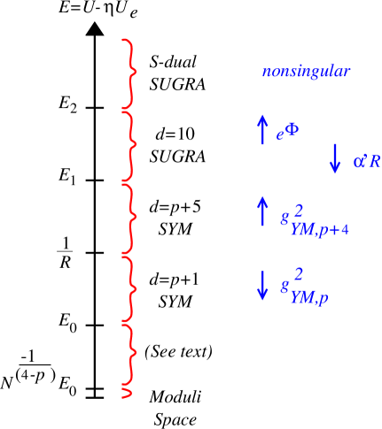
Figure 1: The phase diagram for large-$N$ and $\lambda_{p}R^{3-p}\ll{1}$. Note that when $\lambda_{p}R^{3-p}\gg 1$, the supergravity plus $SU(2)$ gauge description in section 3 should be valid at all radii below $U_{2}$: the two SYM phases and the mystery phase disappear.

To get a little more information on the mystery theory we may consider going to finite temperature, or adding energy to the branes. The first change to the supergravity solution is that a nonextremality function $k(U)$ appears multiplicatively in $g_{tt},g_{UU}^{-1}$:

$$k(U)=1-\left({{U_{0}}\over{U}}\right)^{3-p}\,.$$ (4.19)

In addition, the harmonic function of the D$p$-branes $Z_{p}$ gets altered by nonextremality as if we had not taken the decoupling limit, while $Z_{p+4}$ is unaltered Specifically,

$$Z_{p}\rightarrow 1-{{\xi c_{p+4}\lambda_{p}}\over{(2\pi)^{p-2}U^{3-p}}}\,,$$ (4.20)

where

$$\xi=\left[1+\left({{(2\pi)^{p-2}U_{0}^{3-p}}\over{2c_{p+4}\lambda_{p}}}\right)^{2}\right]^{1/2}-{{(2\pi)^{p-2}U_{0}^{3-p}}\over{2c_{p+4}\lambda_{p}}}\,.$$ (4.21)

Note that $1\geq\xi>0$, and therefore the enhançon at $U=[(1+\xi)/2]U_{\rm e}$ is pulled inwards to smaller $U$ as the ratio $U_{0}^{3-p}/\lambda_{p}$ is increased.

In order for the supergravity horizon at $U=U_{0}$ to lie outside the enhançon locus, we need a sufficiently large energy density $\varepsilon$ on the branes. Using the relation [27] $U_{0}^{3-p}\sim g_{p+4}^{4}\varepsilon$, this implies that

$$\varepsilon R^{p+5}>{{N^{2}}\over{\lambda_{p}R^{3-p}}}\gg 1\,,$$ (4.22)

where we have used the condition (4.10). This cannot be satisfied in the $(p{+}1)$-dimensional gauge theory, and this is further evidence that the mysterious theory is not gravitational.

4.2 The Metric on Moduli Space

Although we have failed to find a weakly coupled dual for the gauge theory, a study of the Coulomb branch of the gauge theory reveals a striking parallel to our probe computations. Focusing on the case $p=2$, suppose that the condition (4.10) holds, so the low energy physics can be described by a $(2+1)$-dimensional gauge theory. The metric that the probe sees, after applying the scaling of the previous section to eqn. (3.16), gives the metric on moduli space for the $SU(N)$ (2+1)-dimensional gauge theory in the decoupling limit:

$${\cal L}=f(U)\left({\dot{U}}^{2}+U^{2}{\dot{\Omega}}^{2}\right)+f(U)^{-1}\left({\dot{\sigma}}-{N\over{8\pi^{2}}}A_{\phi}{\dot{\phi}}\right)^{2}\ ,$$ (4.23)

where

$$f(U)={1\over 8\pi^{2}g^{2}_{\rm YM}}\left(1-{\lambda\over U}\right)\ ,$$ (4.24)

the $U(1)$ monopole potential is $A_{\phi}=\pm 1-\cos\theta,$ and $\sigma=s{\alpha^{\prime}}/2$, and the metric is meaningful only for $U{>}U_{\rm e}=\lambda$. Our metric (4.23) is the Euclidean Taub–NUT metric, with a negative mass. It is a hyperKähler manifold, because $\nabla f=\nabla{\times}A$, where $A=(N/8\pi^{2})A_{\phi}d\phi$.

It is striking that the moduli space metric is the same as that which can be derived from field theory, where this has the interpretation as the tree-level plus one-loop result. It is also interesting to note that while the scaled supergravity solution failed to give a dual, the result for the probe’s moduli space is independent of $V$. Both of these facts could be understood if supersymmetry prevented $V$ from appearing in the probe metric: one can use $V$ as the control parameter to move from weak gauge theory to weak supergravity. On the surface this does not seem to be the case — the probe moduli live in a vector multiplet, and so does $V$ — but a more careful analysis may be needed. So there is a mystery here, perhaps confirming our suggestions in the previous section that there is a useful duality to be found.

We see that the enhançon phenomenon is the same as the familiar fact that the tree-level plus one-loop kinetic term goes negative — the Landau pole. This metric is of course singular, and is therefore incomplete. As shown by Seiberg and Witten, it receives no perturbative corrections but is fixed nonperturbatively. It is the large $r$ expansion of the metric on the moduli space of $N$ monopoles. There are nonperturbative instanton corrections to this metric which smooth it out into a generalization of the Atiyah–Hitchin manifold [29]. In the two-monopole case studies in ref. [30], the Atiyah–Hitchin manifold is the unique smooth completion of the Taub–NUT metric consistent with the condition of hyperKählerity. (See refs. [30, 31, 14, 32] for examples of generalizations and further study.)

To discuss quantitatively the nonperturbative corrections to the metric on moduli space it is simpler to look at the case $p=3$. On the gauge theory side, the metric on moduli space is obtained from the Seiberg–Witten curve [33], which for $SU(N)$ is [34]

$$y^{2}=\prod_{i=1}^{N}(x-\phi_{i})^{2}-\Lambda^{2N}\ .$$ (4.25)

The point of maximal unbroken gauge symmetry, which in the present case can only be the Weyl subgroup, is

$$\phi_{i}=0\ ,\quad\mbox{all $i$}\ .$$ (4.26)

Earlier work on the large-$N$ limit [35] focused on a different point in moduli space, but this highly symmetric point would seem to be the most natural place to look for a supergravity dual. The branch points $y=0$ are at

$$x=\Lambda e^{i\pi k/N}\ ,\quad 0\leq k\leq 2N-1\ .$$ (4.27)

This ring of zeros is reminiscent of the enhançon, and is in fact the same. To see this add a probe brane at $\phi$,

$$y^{2}=x^{2N}(x-\phi)^{2}-\Lambda^{2N+2}\ .$$ (4.28)

For $|\phi|>\Lambda$, there are $2N$ zeros which closely approximate a ring,

$$x\sim\Lambda e^{i\pi k/N}(e^{i\pi k/N}-\phi/\Lambda)^{-1/N}\ ,\quad 0\leq k\leq 2N-1\ ,$$ (4.29)

the new factor, in parentheses, being $1+O(1/N)$. The remaining two zeros are at $x\sim\phi$, or more precisely

$$x\sim\phi\pm(\Lambda/\phi)^{2N}\ ,$$ (4.30)

the correction being exponentially small. On the other hand, for $|\phi|<\Lambda$, all $2N+2$ branch points lie approximately in a ring,

$$x\sim\Lambda e^{i\pi k/(N+1)}(1-\phi e^{-i\pi k/(N+1)}/\Lambda)^{-1/N}\ ,\quad 0\leq k\leq 2N+1\ .$$ (4.31)

As deduced from the string picture, the probe does not penetrate the interior of the enhançon but rather melts into it.

One can extract the moduli space metric from the usual formalism [33, 34]. We leave a more detailed treatment for the future, but in the probe region $\phi>\Lambda$ it matches the perturbative result

$$ds^{2}\sim N\ln\Biggl{(}\frac{U}{\Lambda}\Biggr{)}dud\bar{u}\ .$$ (4.32)

This agrees with the D3-brane probe result on the supergravity side if we identify $\Lambda=\rho_{\rm e}=\sqrt{\rho_{3}\rho_{7}}$.

5 A Tale of Two Duals

As mentioned in the introduction, there are a number of $T$- and $S$- dual pictures where the same physics arises. (The physics of the heterotic $S$-dual for the $p=2$ case is essentially contained in the recent work of ref. [36].)

To construct some $T$-dual cases, consider [14] a pair of NS5-branes which are pointlike in the $(x^{6},x^{7},x^{8},x^{9})$ directions, with $N$ D$(p+1)$-branes stretched between them along the $x^{6}$ direction, where $p=0,1,2$, or 3. The latter are pointlike in the $(x^{p+1},\ldots,x^{5})$ directions, which are inside the NS5-branes, and also in the $(x^{7},x^{8},x^{9})$ directions. All of the branes share the directions $(x^{0},\ldots,x^{p})$. This arrangement of branes, shown in figure 2(a) preserves eight supercharges. We will state the general $p$ case in many of the following formulae. The reader may wish to keep the $p=2$ case in mind for orientation.

                      

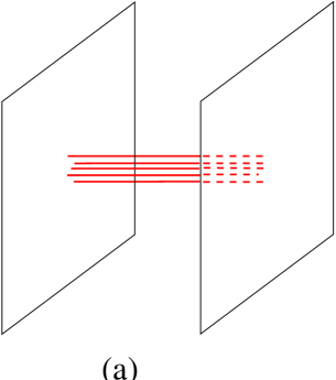
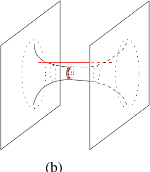
Figure 2: $N$ D$(p+1)$-branes ending on NS5-branes: (a) The classical picture (b) The corrected picture, showing the resulting bending of the NS5-branes for large $gN$. The separated brane is the probe which becomes massless at the enhançon locus, an $S^{4-p}$ (a circle in the figure).

Denoting the separation of the NS5-branes in the $x^{6}$ direction by $L$, there is a $(p+1)$-dimensional $SU(N)$ gauge theory on the infinite part of the world-volume of the D$(p+1)$-branes, whose coupling is

$$g^{2}_{\rm YM}=L^{-1}g^{2}_{p+1}=L^{-1}(2\pi)^{p-1}g\alpha^{\prime(p-2)/2}\ .$$ (5.1)

A number of gauge theory facts from the previous sections are manifest here. For example, the fact that (for $p=2$) the Coulomb branch of the $SU(N)$ gauge theory is dual to the moduli space of $N$ monopoles of a (5+1)-dimensional gauge theory follows from the fact that the ends of the D3-branes are membrane monopole sources (in $x^{3},x^{4},x^{5}$) in the NS5-branes’ world-volume theory. This is an $SU(2)$ gauge theory spontaneously broken to $U(1)$ by the NS5-branes’ separation. This will always be the relevant (5+1)-dimensional theory when $(p+1)$ is odd because we are in type IIB string theory. When $(p+1)$ is even, we are in type IIA, and the (5+1)-dimensional theory is the $A_{1}$ (0,2) theory.

Now place the $x^{6}$ direction on a circle of radius $2\pi\ell$. There is a $T_{6}$-dual of this arrangement of branes. The NS5-branes become an $A_{1}$ ALE space [40]. To see this in supergravity language, we start by smearing the NS5-branes along the $x^{6}$ space, writing the supergravity solution for the core of the NS5-branes as [41] ($|{\bf y}|\gg\ell$):

$$ds^{2} = -dt^{2}+\sum_{m=1}^{5}dx^{m}dx^{m}+H_{5}(dx^{6}dx^{6}+d{\bf y}\cdot d{\bf y})$$

$$e^{2\Phi} = H_{5}(y)={\alpha^{\prime}\over 2\ell}\left({1\over|{\bf y}|}+{1\over|{\bf y}-{\bf y}_{0}|}\right)\ ,$$ (5.2)

where $\bf y$ is a 3-vector in the $(x^{7},x^{8},x^{9})$ plane. We have placed one NS5-brane at ${\bf y}=0$ and the other at ${\bf y}={\bf y}_{0}$. The condition [42, 41] $H_{mns}=\epsilon_{mns}^{\phantom{mns}r}\partial_{r}\Phi$ defines $B_{6i}$ as a vector $\omega_{i}$ which satisfies $\nabla H_{5}=\nabla{\times}{\bf\omega}$. Applying the usual supergravity $T$-duality rules gives:

$$ds^{2} = -dt^{2}+\sum_{m=1}^{5}dx^{m}dx^{m}+H_{5}^{-1}(dx^{6}+\omega_{i}dy^{i})^{2}+H_{5}d{\bf y}\cdot d{\bf y}\ ,$$ (5.3)

which is the two-centre Gibbons–Hawking metric for the $A_{1}$ ALE space, nonsingular because of the $2\pi\alpha^{\prime}/\ell{\equiv}2\pi\ell^{\prime}$ periodicity of $x^{6}$, and hyperKähler because of the condition relating $H_{5}$ and $B_{6i}$ for a supersymmetric fivebrane solution.

There are four moduli associated with this solution, forming a hypermultiplet in the $(5+1)$-dimensional theory. Three of them constitute the vector ${\bf y}_{0}$ giving the separation between the two centres. The fourth is a NS–NS 2-form flux, $\Theta=\int_{{\rm I\!P}^{1}}B_{2}$, through the nontrivial two-cycle (a ${\rm I\!P}^{1}$) in the space. This ${\rm I\!P}^{1}$ is constructed as the locus of $x^{6}$ circles along the straight line connecting the two centres ${\bf y}=0$ and ${\bf y}={\bf y}_{0}$, where they shrink to zero size; it has area $A=2\pi\ell^{\prime}|{\bf y}_{0}|$. These four numbers specify the separation of the two NS5-branes in the $T_{6}$-dual picture.

In our case, we have ${\bf y}_{0}=0$, and so the branes are only separated in $x^{6}$, corresponding to having shrunk the ${\rm I\!P}^{1}$ away. The flux $\Theta$ is kept finite as we send $A$ to zero, and is the parameter dual to $L$:

$$\Theta=2\pi\ell^{\prime}L\,.$$ (5.4)

(The full NS5-branes solution, with dependence on $x^{6}$, can be recovered in the duality by considering winding strings in the ALE geometry [43], doing a sum over those modes which is dual to a Fourier transform of the fivebrane harmonic function on the $x^{6}$ circle.)

On the ALE space, the $W$-bosons for the enhanced $SU(2)$ gauge symmetry of the $(5+1)$-dimensional theory are made from a D2- and an anti D2-brane wrapped on the ${\rm I\!P}^{1}$, their masses being $m=\mu_{2}g^{-1}\sqrt{(2\pi\ell^{\prime})^{2}{\bf y}_{0}\cdot{\bf y}_{0}+\Theta^{2}}$, where the flux appears due to the $\mu_{2}C_{1}{\wedge}B_{2}$ coupling; there is some induced D0-brane charge. Under $T_{6}$-duality, the stretched D$(p+1)$-branes become D$(p+2)$-branes which are wrapped on the ${\rm I\!P}^{1}$, inducing some D$p$-brane charge due to the $\mu_{2}C_{p+1}{\wedge}B_{2}$ coupling.

So the configuration with $N$ D$(p+1)$-branes stretched between the two NS5-branes is dual to the same number of D$(p+2)$-branes wrapped on the two-cycle of an $A_{1}$ ALE space, giving rise to $N$ effective D$p$-branes. The gauge coupling in the resulting $(p+1)$-dimensional $SU(N)$ gauge theory is given by:

$$g^{2}_{\rm YM}=\Theta^{-1}g(2\pi)^{p}\alpha^{\prime(p-1)/2}\ .$$ (5.5)

As mentioned in the introduction, this configuration is $T$-dual to $N$ D$(p~{}+~{}4)$ branes wrapped on a K3, of volume $V$, the parameter dual to $\Theta$. The things we learned about this original configuration translate into refinements of the dual pictures. For example, the nontrivial metric on moduli space corresponds to the bending [44] of the NS5-branes away from being flat, resulting from the D$(p+1)$-branes’ pull on them (See figure 2(b)). Denoting the radial coordinate in the $(x^{p+1},\ldots,x^{5})$ directions as $r$, (as we did before), the $x^{6}$ position of a NS5-brane is given by the equation $\nabla^{2}x^{6}(r)=0$, giving the smooth shape of the NS5-brane for large enough $r$, i.e. far away enough from the details of the junction itself.

The solution for the shape is $x^{6}(r)=\alpha+\beta Nr^{p-3}$ ($p\neq 3$), or $\alpha N\log(r/\beta)$ (for $p=3$), where $\alpha$ and $\beta$ are constants set by $L$, the asymptotic separation of the branes, and $g$ and $\alpha^{\prime}$. Using this, an expression for the separation $L(r)$ of the NS5-branes is

$$L(r) = L-{2\beta N\over r^{3-p}};\quad(p\neq 3)\ ,$$

$$L(r) = 2\alpha N\log\left({r\over\beta}\right);\quad(p=3)\ .$$ (5.6)

Notice that this is precisely the functional behavior that we see in the harmonic functions for the supergravity solution of the D$p$-D$(p+4)$ system. The parameters $\alpha$ and $\beta$ can be fixed completely by comparing to the large $r$ limit of probe moduli space computation done there, although we will not do it here.

In the expression (5.1) for the gauge coupling, we should replace $L$ by our expression for $L(r)$, giving the running of the coupling with position on the Coulomb branch.

We recover therefore the singularity in the Coulomb branch where the gauge coupling diverges, when the separation $L(r)$ of the NS5-branes is of order $\alpha^{\prime}$, resulting in an enhanced gauge symmetry on the NS5-branes’ (5+1)-dimensional world-volume. The enhançon is simply the $S^{4-p}$ of closest approach of the NS5-branes in the $x^{6}$ direction. Notice that the probe brane we studied previously is a single stretched D$(p+1)$-brane moving in $(x^{p+1},\ldots,x^{5})$ in this picture.

An $r$-dependence in the separation between the NS5-branes translates, using (5.4), into variable $W$-boson masses $m=\mu_{2}g^{-1}\Theta(r)$ in the $(5+1)$-dimensional theory, giving the enhançon locus where $\Theta(r)$ vanishes. Using $\Theta(r)$ in the formula (5.5) results in the divergence in the $(p+1)$-dimensional gauge coupling at the enhançon locus.

6 Conclusions

One notable result of this paper is a new mechanism that resolves a large class of spacetime singularities in string theory. This involves a phenomenon, the resolution of a singularity by the expansion of a system of branes in the transverse directions, which is related to that which has recently arisen in other forms [45, 46]. One difference from [45] is that the branes are found not at the singularity in the supergravity metric; rather, the metric is modified by string/braney phenomena in the manner that we have described. Our result may point toward a more general understanding of singularities in string theory.

In the gauge theory we have found a striking parallel between the spacetime picture and the behavior of large-$N$ $SU(N)$ gauge theories. The most interesting open question is to find a weakly coupled dual to the strongly coupled gauge theory; our results give many hints in this direction. There are a number of technical loose ends, which include a more complete treatment of the D3-D7 case, and a fuller understanding of the constraints of supersymmetry on the probe moduli space. Finally, there are many interesting generalizations, including product gauge groups, the addition of hypermultiplets, and rotation.

References

- [1] L. Dixon, J.A. Harvey, C. Vafa and E. Witten, Nucl. Phys. B261, 678 (1985).
-
[2]
E. Witten,
Nucl. Phys. B403, 159 (1993)
hep-th/9301042;
P.S. Aspinwall, B.R. Greene and D.R. Morrison, Phys. Lett. B303, 249 (1993) hep-th/9301043. -
[3]
P. Candelas, P.S. Green and T. Hubsch,
Phys. Rev. Lett. 62, 1956 (1989);
A. Strominger, Nucl. Phys. B451, 96 (1995) hep-th/9504090;
B.R. Greene, D.R. Morrison and A. Strominger, Nucl. Phys. B451, 109 (1995) hep-th/9504145. - [4] G.T. Horowitz and R. Myers, Gen. Rel. Grav. 27, 915 (1995) gr-qc/9503062.
- [5] K. Behrndt, Nucl. Phys. B455, 188 (1995) hep-th/9506106.
- [6] R. Kallosh and A. Linde, Phys. Rev. D52, 7137 (1995) hep-th/9507022.
- [7] M. Cvetič and D. Youm, Phys. Lett. B359, 87 (1995) hep-th/9507160.
- [8] J. Maldacena, Adv. Theor. Math. Phys. 2, 231 (1998) hep-th/9711200.
- [9] M. Bershadsky, C. Vafa and V. Sadov, Nucl. Phys. B463, 398 (1996) hep-th/9510225.
- [10] S. Kachru and E. Silverstein, Phys. Rev. Lett. 80, 4855 (1998) hep-th/9802183.
- [11] J. Polchinski, Phys. Rev. D55, 6423 (1997) hep-th/9606165.
- [12] C.V. Johnson and R.C. Myers, Phys. Rev. D55, 6382 (1997) hep-th/9610140.
-
[13]
M.R. Douglas,
JHEP 07, 004 (1997)
hep-th/9612126;
D. Diaconescu, M.R. Douglas and J. Gomis, JHEP 02, 013 (1998) hep-th/9712230. - [14] A. Hanany and E. Witten, Nucl. Phys. B492, 152 (1997) hep-th/9611230.
- [15] C.V. Johnson, N. Kaloper, R.R. Khuri and R.C. Myers, Phys. Lett. B368, 71 (1996) hep-th/9509070.
-
[16]
R.D. Sorkin,
Phys. Rev. Lett. 51, 87 (1983);
D.J. Gross and M.J. Perry, Nucl. Phys. B226, 29 (1983). -
[17]
R.R. Khuri,
Phys. Lett. B294, 325 (1992)
hep-th/9205051;
R.R. Khuri, Nucl. Phys. B387, 315 (1992) hep-th/9205081. - [18] M.J. Duff, R.R. Khuri, R. Minasian and J. Rahmfeld, Nucl. Phys. B418, 195 (1994) hep-th/9311120.
-
[19]
S.S. Gubser and I.R. Klebanov,
Phys. Rev. D58, 125025 (1998)
hep-th/9808075;
I.R. Klebanov and N.A. Nekrasov, hep-th/9911096. - [20] M. Green, J.A. Harvey and G. Moore, Class. Quant. Grav. 14, 47 (1997) hep-th/9605033.
- [21] K. Dasgupta, D.P. Jatkar and S. Mukhi, Nucl. Phys. B523, 465 (1998) hep-th/9707224.
- [22] C.P. Bachas, P. Bain and M.B. Green, JHEP 05, 011 (1999) hep-th/9903210.
- [23] R. Gopakumar and C. Vafa, hep-th/9811131.
- [24] L. Alvarez-Gaume and D.Z. Freedman, Commun. Math. Phys. 80, 443 (1981).
- [25] P.K. Townsend, Phys. Lett. B373, 68 (1996) hep-th/9512062.
- [26] C. Schmidhuber, Nucl. Phys. B467, 146 (1996) hep-th/9601003.
- [27] N. Itzhaki, J.M. Maldacena, J. Sonnenschein and S. Yankielowicz, Phys. Rev. D58, 046004 (1998) hep-th/9802042.
- [28] C. Vafa, Nucl. Phys. B469, 403 (1996)
- [29] M.F. Atiyah and N.J. Hitchin, “The Geometry And Dynamics Of Magnetic Monopoles. M.B. Porter Lectures”, Princeton University Press (1988).
- [30] N. Seiberg and E. Witten, hep-th/9607163.
- [31] G. Chalmers and A. Hanany, Nucl. Phys. B489, 223 (1997) hep-th/9608105.
- [32] N. Dorey, V.V. Khoze, M.P. Mattis, D. Tong and S. Vandoren, Nucl. Phys. B502, 59 (1997) hep-th/9703228. hep-th/9602022.
- [33] N. Seiberg and E. Witten, Nucl. Phys. B426, 19 (1994) hep-th/9407087.
-
[34]
P.C. Argyres and A.E. Faraggi,
Phys. Rev. Lett. 74, 3931 (1995)
hep-th/9411057;
A. Klemm, W. Lerche, S. Yankielowicz and S. Theisen, Phys. Lett. B344, 169 (1995) hep-th/9411048. - [35] M.R. Douglas and S.H. Shenker, Nucl. Phys. B447, 271 (1995) hep-th/9503163.
- [36] M. Krogh, hep-th/9911084.
- [37] C.V. Johnson, Nucl. Phys. B507, 227 (1997) hep-th/9706155.
- [38] A. Karch, D. Lust and D. Smith, Nucl. Phys. B533, 348 (1998) hep-th/9803232.
- [39] K. Dasgupta and S. Mukhi, JHEP 07, 008 (1999) hep-th/9904131.
-
[40]
E. Witten,
hep-th/9507121;
H. Ooguri and C. Vafa, Nucl. Phys. B463, 55 (1996) hep-th/9511164. - [41] J.P. Gauntlett, J.A. Harvey and J.T. Liu, Nucl. Phys. B409, 363 (1993) hep-th/9211056.
-
[42]
A. Strominger,
Nucl. Phys. B343, 167 (1990);
S. Rey, Phys. Rev. D43, 526 (1991);
C.G. Callan, J.A. Harvey and A. Strominger, hep-th/9112030. - [43] R. Gregory, J.A. Harvey and G. Moore, Adv. Theor. Math. Phys. 1, 283 (1997) hep-th/9708086.
- [44] E. Witten, Nucl. Phys. B500, 3 (1997) hep-th/9703166.
-
[45]
P. Kraus, F. Larsen and S.P. Trivedi,
JHEP 03, 003 (1999)
hep-th/9811120;
D.Z. Freedman, S.S. Gubser, K. Pilch and N.P. Warner, hep-th/9906194;
A. Brandhuber and K. Sfetsos, hep-th/9906201. -
[46]
R.C. Myers,
hep-th/9910053;
J. Polchinski and M. Strassler, in progress;
S.S. Gubser, K. Pilch and N.P. Warner, in progress.