SMI-5-99 On Stable Sector in Supermembrane Matrix Model

Abstract

We study the spectrum of $SU(2)\times SO(2)$ matrix supersymmetric quantum mechanics. We use angular coordinates that allow us to find an explicit solution of the Gauss law constrains and single out the quantum number $n$ (the Lorentz angular momentum). Energy levels are four-fold degenerate with respect to $n$ and are labeled by $n_{q}$, the largest $n$ in a quartet. The Schrödinger equation is reduced to two different systems of two-dimensional partial differential equations. The choice of a system is governed by $n_{q}$. We present the asymptotic solutions for the systems deriving thereby the asymptotic formula for the spectrum. Odd $n_{q}$ are forbidden, for even $n_{q}$ the spectrum has a continuous part as well as a discrete one, meanwhile for half-integer $n_{q}$ the spectrum is purely discrete. Taking half-integer $n_{q}$ one can cure the model from instability caused by the presence of continuous spectrum.

1 Introduction

Supersymmetric quantum mechanics describing an $SO(d)$ invariant interaction of $d$ $SU(n)$-matrices has attracted a lot of attention in the last two decades.

The original interest to this model was caused by its description of $1+0$ reduction of $1+d$ dimensional supersymmetric $SU(n)$ gauge theory. A reduction of non-supersymmetric $d=3$ Yang-Mills theory to a mechanical model was considered in the pioneering papers [1]. It was noticed that already for the simplest case of $SU(2)$ gauge group one gets a rather complicated mechanical system with 9 degrees of freedom [2]. This mechanical system was investigated only within the special ansatze. Within one of them the model is reduced to a model with two degrees of freedom which is still rather non-trivial and exhibits a chaotic behaviour [1, 3] in the classical case . Later on, this model has been investigated in the quantum case. It was also proved that this system has a discrete spectrum [4, 5]. This spectrum possesses a very interesting property – it is in some sense a direct product of two harmonic oscillators [6]. The possible applications for realistic models see [7].

In the end of 80-th the interest to the matrix quantum mechanics was inspired by an observation that it describes a regularised membrane theory in $d+2$ space-time dimensions [8, 9, 10, 11]. The membrane theory was supposed to be reached in the limit of large $n$. Since the membranes were considered within the 11 dimensional supergravity the supersymmetric version of $SU(n)\times SO(9)$ quantum mechanics has to be examined. In contrast to the bosonic matrix models where the spectrum is purely discrete, in supermembrane matrix models a continuous spectrum, filling the positive half of the real line was detected [11]. This fact was considered as a manifestation of the instability of the supermembrane against deformations into stringlike configurations.

Let us also note that more early, in the beginning of the 80’s supersymmetric quantum mechanics (SQM) was proposed as a model for better understanding of supersymmetry breaking [12]. In this context SQM was considered in [13, 14, 15]. This model is essentially simpler as compare to the membrane super quantum mechanics, since its bosonic part has only one degree of freedom.

A renovation of interest to a supersymmetric matrix quantum mechanics in the last three years was motivated by its relation to a description of the dynamics of D-0 branes in superstring theory [16, 17]. Moreover, this model in the large $n$ limit pretends to the role of M-theory [18]. This conjecture has stipulated the recent study of $SU(n)\times SO(d)$ supersymmetric quantum mechanics [19]-[21]. Within M-theory there is a very important question of the existence of normalized eigenfunctions with zero energy, since the zero modes represent the graviton multiplet of eleven dimensional supergravity. This problem has attracted attention since the first paper where the model was introduced. One expected that $SU(n)\times SO(d)$ supersymmetric quantum mechanics has one normalized zero-mode for $d=9$, and has none for $d=2,3,5$ (only in these dimensions a supersymmetric model can be formulated) [19]-[33].

The case of large $n$ is rather involved. The simplest case is the $SU(2)$ one. In this context the $SU(2)$ quantum mechanics was investigated in [19, 20, 21]. The case of arbitrary $n$ was considered in [27, 28, 30] and $n=3$ was considered in [33]. To investigate the zero-mode problem the Born-Oppenheimer approximation was applied [19, 20, 21]. This method allows to find asymptotic behaviour near ”infinity”. Therefore, if one does not expect any singularities at a finite region, one can deduce an existence/nonexistence of normalized zero-mode from asymptotic behaviour. An effective tool to study the zero-mode problem is an investigation of a system of first order differential equations caused by the supersymmetry of a desired zero mode. The Born-Oppenheimer approximation is also applicable to the study of the first order differential equations. Recently the authors of [32] have performed an investigation of zero-mode problem using the first order differential equation. The asymptotic behaviour found in [32] supports a common belief about the existence of normalized zero-mode in $d=9$ and nonexistence in other dimensions.

Let us make few comments about chaotic behaviour of matrix models. About classical dynamics of two-dimensional model [1] see [34, 35]. Classical dynamics in bosonic membrane matrix model was investigated and a chaotic behaviour was demonstrated. Later on, in $SU(2)\times SO(2)$ matrix model a classical chaos-order transition was found [36, 37]. For the Lorentz momentum $N$ small enough (even for small coupling constant) the system exhibits a chaotic behaviour, for $N$ large enough the system is regular. Up to now the question of similar transition in quantum case remains open. $\alpha^{\prime}$-corrections to the Yang-Mills approximation of D-particle dynamics were studied in [38] where a stabilization of the classical trajectories was shown.

The main task of this paper is to find the whole spectrum of $SU(2)\times SO(2)$ supersymmetric matrix quantum mechanics. In the previous investigations of this model the following particular results about the spectrum were obtained. Continuous spectrum was observed [11] and the nonexistence of normalized zero mode has been proved [23]. The character of spectrum plays an important role in stability/instability of the system. Let us remind that according to the commonly accepted opinion this model is unstable. The potential instability of (super) matrix quantum mechanics is evident from classical consideration. Namely, the potential of matrix models has valleys through which a part of coordinates can escape to infinity without increasing the energy. For the bosonic case the classical instability is cured by quantum fluctuations due to which the flat directions become closed by confined potentials, so that finite energy wave functions fall off rapidly and spectrum is purely discrete [6, 4], that provides stability. The lost of stability in supersimmetric case is caused by additional contributions to the potential coming from the fermionic degrees of freedom which cancel the bosonic ones. As a result of this cancellation wave functions are no more confined and the spectrum becomes continuous [11]. This cancellation takes place on special states, that means a coexistence of the continuous spectrum and the discrete one. To specify states for which a cancellation/non cancellation takes place it is convenient to arrange the states into quartets enumerated by a number $n_{q}$. Upon quantization $n_{q}$ can be integer or half-integer. Our analysis of $SU(2)\times SO(2)$ supersymmetric quantum mechanics shows that there is a cancellation in the sector with even $n_{q}$ and there is no cancellation for half-integer $n_{q}$ (states with odd $n_{q}$ are forbidden). As a result, there is only a discrete spectrum in the half-integer $n_{q}$ sector and the model is stable. The lowest energy in this sector is positive, that means the supersymmetry is broken in this sector.

Our main tool in the detailed study of the spectral problem of $SU(2)\times SO(2)$ supersymmetric quantum mechanics is the proper coordinates, four angles $\gamma_{1}$ ,$\gamma_{2}$, $\alpha$, $\theta$ and two radii $f$ and $g$. These coordinates have been already used in [36]. In these coordinates we will find an explicit solution to the Gauss law constrains and single out quantum number $n$. Due to this parametrisation the spectral problem for a supersymmetric version of the model with 6 degrees of freedom will be reduced to a pair of systems of partial differential equations in $f$ and $g$. The choice of a system is dictated by the value of $n_{q}$. For half-integer $n_{q}$ we have just one equation on one function of $f$ and $g$. For even $n_{q}$ we have three equations on three functions of $f$ and $g$.

We present asymptotic solutions of these two systems deriving thereby the asymptotic formula for the spectrum. For half-integer $n_{q}$ we deal with differential operator corresponding to standard potential problem in quantum mechanics and character of the spectrum can be understood from the form of potential. Since we have a confining potential the spectrum is discrete. We present an asymptotic solution of the Schrödinger equation and corresponding formula for the spectrum. For even $n_{q}$ we have a matrix second order differential operator. Just for this system a vanishing of the bosonic confining potential takes place on special states and the matrix differential operator has the continuous spectrum. To get it we find the asymptotic solution of the system of three equations. Besides the continuous spectrum this operator possesses the discrete spectrum. States with integer (half-integer) $n$ belong to the stable sector if they satisfy the constraint $Q\Psi_{n}=0$ ($\bar{Q}\Psi_{n}=0$).

The paper is organised as follows. In Section 2 we explore the algebraic structure of $SU(2)\times SO(2)$ supersymmetric quantum mechanics in context of energy level degeneracy. In Section 3 we specify the angular $SU(2)\times SO(2)$ parametrization. A special attention is spared to generalized periodicity. In Section 4 we solve the constrains in the angular parametrization and present the spectral problem as two sets of two-dimensional partial differential equations. In Section 5 the spectrum of corresponding differential operators is examined. We present asymptotic solutions of the Schrödinger equation and corresponding formula for the spectrum.

2 Algebraic Structure of $SU(2)\times SO(2)$ Supersymmetric Quantum Mechanics

2.1 The Hamiltonian and Superalgebra

We consider the system described by the Hamiltonian

$$H = H_{B}+H_{F},$$ (1)

$$H_{B} = \frac{g_{s}}{2}(\pi_{1}^{2}+\pi_{2}^{2})+\frac{1}{2g_{s}}\left|\varphi_{1}\times\varphi_{2}\right|^{2},$$

$$H_{F} = -\frac{i}{2}\varepsilon^{abc}\left(\varphi_{1}^{a}+i\varphi_{2}^{a}\right)\chi^{b}\chi^{c}-\frac{i}{2}\varepsilon^{abc}\left(\varphi_{1}^{a}-i\varphi_{2}^{a}\right)\bar{\chi}^{b}\bar{\chi}^{c}$$

and constrained by the Gauss law $j^{a}|\Psi\rangle=0$. $\pi_{i}^{a}$, $\varphi_{j}^{b}$ and $\bar{\chi}^{a}$, $\chi^{b}$ are canonically conjugated pairs with

$$\left[\pi_{i}^{a},\varphi_{j}^{b}\right]=-i\delta^{ab}\delta_{ij},~{}~{}~{}\left\{\bar{\chi}^{a}\chi^{b}\right\}=\delta^{ab}.$$ (2)

The Hamiltonian (1) is invariant under $SU(2)$ rotations and redundant Lorentz rotation generated by

$$j^{a}=l^{a}+s^{a}, l^{a}=\varepsilon^{abc}\varphi_{i}^{b}\pi_{i}^{c},~{}~{}s^{a}=-i\varepsilon^{abc}\bar{\chi}^{b}\chi^{c},$$ (3)

$$N=N_{B}+N_{F}, N_{B}=\varphi_{1}^{a}\pi_{2}^{a}-\varphi_{2}^{a}\pi_{1}^{a},~{}~{}N_{F}=\frac{1}{2}\bar{\chi}^{a}\chi^{a}$$ (4)

respectively. The commutation relations for the currents read:

$$\left[j^{a},j^{b}\right]=i\varepsilon^{abc}j^{c},~{}~{}\left[j^{a},N\right]=0.$$

There are two supercharges:

$$Q=-\frac{\sqrt{g_{s}}}{\sqrt{2}}\bar{\chi}^{a}(\pi_{1}^{a}-i\pi_{2}^{a})+\frac{i}{\sqrt{2g_{s}}}\chi^{a}\varepsilon^{abc}\varphi_{1}^{b}\varphi_{2}^{c},$$ (5)

$$\bar{Q}=-\frac{\sqrt{g_{s}}}{\sqrt{2}}\chi^{a}(\pi_{1}^{a}+i\pi_{2}^{a})-\frac{i}{\sqrt{2g_{s}}}\bar{\chi}^{a}\varepsilon^{abc}\varphi_{1}^{b}\varphi_{2}^{c}$$ (6)

and

$$\left\{Q,\bar{Q}\right\}=H.$$

The supercharges commute with the Hamiltonian up to the generator of $SU(2)$ rotations vanishing on the physical states.

The remaining commutators with $Q$ and $\bar{Q}$ are the following:

$$Q^{2} = 0,~{}~{}~{}\bar{Q}^{2}=0,$$ (8)

$$\left[Q,j^{a}\right] = \left[\bar{Q},j^{a}\right]=0,$$

$$\left[N,Q\right] = -\frac{1}{2}Q,$$

$$\left[N,\bar{Q}\right] = \frac{1}{2}\bar{Q},$$

$$\left[N,H\right] = 0.$$ (9)

Note, that the algebra (8)-(9) is not affected by a shift of $N$ by a constant. As compare with [32] our $N$ is shifted on $1/4$.

2.2 Energy Level Degeneration

2.2.1 The Algebra

On the physical states ($j^{a}|\Psi\rangle=0$) there are three operators commuting with $H$: $Q$, $\bar{Q}$ and $N$. This provides the degeneration of energy levels. In this section we discuss the irreducible representations $v_{E}$ of the algebra (8) - (9) for a non-zero energy $E$.

Lemma. Let $|\Psi\rangle\in v_{E}$ with $E\neq 0$ be an eigenvector of $H$ and $N$, then $Q|\Psi\rangle=0$ or $\bar{Q}|\Psi\rangle=0$.

Proof. Suppose that $Q|\Psi\rangle\neq 0$ and $\bar{Q}|\Psi\rangle\neq 0$ then one has two additional eigenvectors of $N$ with the same energy:

$$N(Q|\Psi\rangle) = (n-\frac{1}{2})(Q|\Psi\rangle),$$ (10)

$$N(\bar{Q}|\Psi\rangle) = (n+\frac{1}{2})(\bar{Q}|\Psi\rangle).$$ (11)

One can check, that the operator

$$K=HN+\frac{1}{4}[Q,\bar{Q}]$$

is one more Casimir of the algebra (8) - (9). By a simple calculation one finds:

$$K|\Psi\rangle = E(n+\frac{1}{4})|\Psi\rangle-\frac{1}{2}\bar{Q}Q|\Psi\rangle=E(n-\frac{1}{4})|\Psi\rangle+\frac{1}{2}Q\bar{Q}|\Psi\rangle,$$ (12)

$$K(Q|\Psi\rangle) = E(n-\frac{1}{4})(Q|\Psi\rangle),$$ (13)

$$K(\bar{Q}|\Psi\rangle) = E(n+\frac{1}{4})(\bar{Q}|\Psi\rangle).$$ (14)

For $v_{E}$ to be irreducible the value of the Casimir on $|\Psi\rangle$ should be equal to its value on $Q|\Psi\rangle$ and $\bar{Q}|\Psi\rangle$.  From equations (12)-(14) we see that this requires

$$Q|\Psi\rangle=0~{}~{}~{}\mbox{or}~{}~{}~{}\bar{Q}|\Psi\rangle=0.$$

Since $\bar{Q}$ and $Q$ act as raising and lowering operators (eqs.(10), (11)) one can introduce a label: $v_{E,n}$ where $n$ is the value of $N$ on the vector $|\Psi\rangle\in\ker\bar{Q}$.

So, we find that $v_{E,n}$ is a vector space spanned by two eigenvectors of $N$: $|\Psi_{1}\rangle$ and $|\Psi_{2}\rangle$ such that

$$\bar{Q}|\Psi_{1}\rangle=0=Q|\Psi_{2}\rangle$$

and

$$N|\Psi_{1}\rangle=n|\Psi_{1}\rangle,~{}~{}~{}N|\Psi_{2}\rangle=(n-\frac{1}{2})|\Psi_{2}\rangle.$$

2.2.2 Discrete Symmetry

In addition to the algebra (8) - (9) the Hamiltonian (1) admits one more symmetry. The bosonic part of the Hamiltonian is invariant under the discrete transformation

$$\varphi_{1}\longleftrightarrow\varphi_{2}.$$ (15)

To extend this symmetry for the supersymmetric case we put:

$$\chi\to\mu\bar{\chi}$$ (16)

$$\bar{\chi}\to\nu\chi.$$ (17)

The invariance of the Hamiltonian and of the commutation relations gives the following restrictions on $\mu,\nu$:

$$-\mu^{2}=\nu^{2}=i,$$ (18)

$$\mu\nu=1.$$ (19)

One more restriction:

$$\nu=i\mu$$

comes from imposing the condition for transformation law of supercharges $Q,\bar{Q}$ to be homogeneous.

The system of equations for $\mu$ and $\nu$ has a solution (up to an overall sign):

$$\mu=e^{-i\frac{\pi}{4}},~{}~{}~{}\nu=e^{i\frac{\pi}{4}}.$$

Denote the operator generating this symmetry by $P$, then we have

$$[P,H]=0,~{}~{}~{}[P,j]=0,$$ (20)

$$PQ-\mu\bar{Q}P=0,~{}~{}~{}P\bar{Q}-\nu QP=0,$$

$${}\{P,N\}=\frac{3}{2}P,$$

$$P^{2}=1.$$ (21)

Note, that $P$ acts on the spinor monomials without permutations of spinor factors, because these permutations are incompatible with the invariance of the anticommutation relations (2).

Figure 1: States in a quartet $n_{q}=n$

As $Pv_{E,n}=v_{E,2-n}$ (action of $P$-operator on the states will be specified below) the irreducible representations of the enlarged algebra (8)-(9)+(20)-(21) are direct sums: $V_{E,n_{q}}=v_{E,n}+v_{E,2-n}$, where $n_{q}$ is the maximal number of $n$ and $2-n$. To avoid doublecounting one has to restrict the range for $n$ as to exclude $n<-n+2$ which gives $n>1$. In the exceptional case $n=1$: $v_{E,1}=v_{E,-1+2}$, i.e. for $n=1$ one has a two-dimensional instead of a four-dimensional irreducible representation. The further specification of the range will be given below.

2.3 Action of $P$-operator on the States

A general wave function is a vector of the eight-dimensional fermionic Fock space based on the fermionic vacuum $|0\rangle$: $\chi^{a}|0\rangle=0$. It is useful to arrange the fermionic states according to their parity as follows:

$$|\Psi\rangle=\left(\psi_{0}+\psi^{1}\bar{\chi}^{2}\bar{\chi}^{3}+\psi^{2}\bar{\chi}^{3}\bar{\chi}^{1}+\psi^{3}\bar{\chi}^{1}\bar{\chi}^{2}+\ \tilde{\psi}_{0}\bar{\chi}^{1}\bar{\chi}^{2}\bar{\chi}^{3}+\tilde{\psi}^{1}\bar{\chi}^{1}+\tilde{\psi}^{2}\bar{\chi}^{2}+\tilde{\psi}^{3}\bar{\chi}^{3}\right)|0\rangle,$$ (22)

where $\psi_{0}$, $\psi^{a}$, $\tilde{\psi}_{0}$ and $\tilde{\psi}^{a}$ are some functions of $\vec{\varphi}_{1}$, $\vec{\varphi}_{2}$. The Fock space can also be created by operators $\bar{\chi}^{a}$ acting on the ”dual” vacuum

$$|0)=\bar{\chi}^{1}\bar{\chi}^{2}\bar{\chi}^{3}|0\rangle.$$

To define the action of $P$ on $|\Psi\rangle$ one has to specify the action of $P$ on the vacuum $|0\rangle$ (or on $|0)$). The unique choice that gives non-degenerate $P$ is:

$$P|0\rangle=\lambda|0),$$ (23)

where $\lambda$ is some numerical factor to be fixed by the constraint $P^{2}=1$.

It is instructive to represent $|\Psi\rangle$ as a column of $\psi$-s with the ordering dictated by eq.(22). Within this notation one can write:

$$P^{2}|\Psi\rangle=P^{2}\left(\begin{array}[]{l}\psi_{0}\\ \psi^{1}\\ \psi^{2}\\ \psi^{3}\\ \tilde{\psi}_{0}\\ \tilde{\psi}^{1}\\ \tilde{\psi}^{2}\\ \tilde{\psi}^{3}\end{array}\right)_{(1,2)}=\lambda P\left(\begin{array}[]{l}\tilde{\psi}_{0}(-\nu^{3})\\ \tilde{\psi}^{1}\nu\\ \tilde{\psi}^{2}\nu\\ \tilde{\psi}^{3}\nu\\ \psi_{0}\\ \psi^{1}(-\nu^{2})\\ \psi^{2}(-\nu^{2})\\ \psi^{3}(-\nu^{2})\end{array}\right)_{(2,1)}=-\lambda^{2}\nu^{3}\left(\begin{array}[]{l}\psi_{0}\\ \psi^{1}\\ \psi^{2}\\ \psi^{3}\\ \tilde{\psi}_{0}\\ \tilde{\psi}^{1}\\ \tilde{\psi}^{2}\\ \tilde{\psi}^{3}\end{array}\right)_{(1,2)},$$ (24)

where labels $(1,2)$, $(2,1)$ indicate the order of bosonic arguments for $\psi$-s.

The constraint $P^{2}=1$ results in $-\lambda^{2}\nu^{3}=1$ and gives, according to our choice of $\nu$ :

$$\lambda=e^{i\frac{\pi}{8}}.$$

In a matrix form the action of the operator $P$ on the fermionic degrees of freedom can be represented as follows

$$P=\lambda\left(\begin{array}[]{cc}0&\begin{array}[]{cccc}1&0&0&0\\ 0&-\nu^{2}&0&0\\ 0&0&-\nu^{2}&0\\ 0&0&0&-\nu^{2}\\ \end{array}\\ \begin{array}[]{cccc}-\nu^{3}&0&0&0\\ 0&\nu&0&0\\ 0&0&\nu&0\\ 0&0&0&\nu\end{array}&0\\ \end{array}\right).$$ (25)

2.4 Gauss Law and $N|\Psi\rangle=n|\Psi\rangle$ in Components

The Gauss law

$$j^{a}|\Psi\rangle=0$$

fixes the $SU(2)$ transformation properties of the component wave functions $\psi^{a}$, $\tilde{\psi}^{a}$. These are given by:

$$l^{a}|\Psi\rangle=-s^{a}|\Psi\rangle.$$

The spin operator $\vec{s}$ acts on fermionic Fock states and its action can be easily calculated to give

$$[l^{a},\psi_{0}] = 0,$$

$${}[l^{a},\psi^{b}] = i\epsilon^{abc}\psi^{c},$$

$${}[l^{a},\tilde{\psi}_{0}] = 0,$$ (26)

$${}[l^{a},\tilde{\psi}^{b}] = i\epsilon^{abc}\tilde{\psi}^{c}.$$

Hence, we conclude that: 1) $\psi_{0}$ and $\tilde{\psi}_{0}$ are $SU(2)$ singlets, 2) $\vec{\psi}=(\psi^{1},\psi^{2},\psi^{3})$ and $\vec{\tilde{\psi}}=(\tilde{\psi}^{1},\tilde{\psi}^{2},\tilde{\psi}^{3})$ are $SU(2)$ triplets. One can check that

$${\vec{l}}^{2}\psi_{0}={\vec{l}}^{2}\tilde{\psi}_{0}=0,$$

$$[\vec{l}^{2},\vec{\psi}]=2\vec{\psi},~{}~{}~{}~{}[\vec{l}^{2},\vec{\tilde{\psi}}]=2\vec{\tilde{\psi}}$$

as it must be for the scalar and vector representation. The explicit solution of (26) will be given below after the parametrisation of the configuration space $(\vec{\varphi_{1}},\vec{\varphi_{2}})$ will be specified.

In the following we shall exploit the eigenstates of $N$. It is instructive to separate the fermion number operator $N_{F}$. Let: $N|\Psi\rangle=n|\Psi\rangle$ then $N_{B}|\Psi\rangle=(n-N_{F})|\Psi\rangle$ gives

$$N_{B}\psi_{0} = n\psi_{0},$$

$$N_{B}\vec{\psi} = (n-1)\vec{\psi},$$

$$N_{B}\tilde{\psi}_{0} = (n-\frac{3}{2})\tilde{\psi}_{0},$$ (27)

$$N_{B}\vec{\tilde{\psi}} = (n-\frac{1}{2})\vec{\tilde{\psi}}.$$

2.5 Shrödinger equation in components

The fermionic Fock space decomposition (22) for $|\Psi\rangle$ provides a matrix representation for Shrödinger equation $H|\Psi\rangle=E|\Psi\rangle$. Taking $|\Psi\rangle$ as a column (see (24)) one deduces $H$ in a block-diagonal form:

$$H=\left(\begin{array}[]{cc}\begin{array}[]{cccc}H_{B}&i\varphi^{1}&i\varphi^{2}&i\varphi^{3}\\ -i\bar{\varphi}^{1}&H_{B}&0&0\\ -i\bar{\varphi}^{2}&0&H_{B}&0\\ -i\bar{\varphi}^{3}&0&0&H_{B}\\ \end{array}&0\\ 0&\begin{array}[]{cccc}H_{B}&-i\bar{\varphi}^{1}&-i\bar{\varphi}^{2}&-i\bar{\varphi}^{3}\\ i\varphi^{1}&H_{B}&0&0\\ i\varphi^{2}&0&H_{B}&0\\ i\varphi^{3}&0&0&H_{B}\\ \end{array}\end{array}\right),$$ (28)

where

$$\varphi^{a}=\varphi^{a}_{1}+i\varphi^{a}_{2},~{}~{}\bar{\varphi}^{a}=\varphi^{a}_{1}-i\varphi^{a}_{2}.$$ (29)

On physical states ($\vec{j}|\Psi\rangle=0$) the component equations for $SU(2)$ triplet $\vec{\psi}$ ($\vec{\tilde{\psi}}$) are not independent. For instance, the last equation for the upper block is (equation number four):

$$-i\bar{\varphi}^{3}\psi_{0}+H_{B}\psi^{3}=E\psi^{3}.$$ (30)

Let us apply $l^{1}$ to (30):

$$-il^{1}(\bar{\varphi}^{3}\psi_{0})+l^{1}(H_{B}\psi^{3})=El^{1}\psi^{3},$$

then by using the commutation relations (26) and $[l^{a},\varphi^{b}]=i\varepsilon^{abc}\varphi^{c}$ one gets the third Shrödinger equation

$$-i\bar{\varphi}^{2}\psi_{0}+H_{B}\psi^{2}=E\psi^{2}$$

and so on.

Therefore, we are left with two sets of equations:

$$\left\{\begin{array}[]{l}H_{B}\psi_{0}+i(\vec{\varphi}\vec{\psi})=E\psi_{0}\\ H_{B}\psi^{3}-i\bar{\varphi}^{3}\psi_{0}=E\psi^{3}\end{array}\right.$$ (31)

and

$$\left\{\begin{array}[]{l}H_{B}\tilde{\psi}_{0}-i(\vec{\bar{\varphi}}\vec{\tilde{\psi}})=E\tilde{\psi}_{0}\\ H_{B}\tilde{\psi}^{3}+i\varphi^{3}\tilde{\psi}_{0}=E\tilde{\psi}^{3}\end{array}\right.$$ (32)

with $\psi^{1,2}$ ($\tilde{\psi}^{1,2}$) expressed in terms of $\psi^{3}$ ($\tilde{\psi}^{3}$).

3 $SU(2)\times SO(2)$ Parametrisation

3.1 Parametrisation

We parametrise the configuration space $\{\varphi_{i}^{a}\}$ by using the new coordinates $\{f,g,\theta,\gamma_{1},\gamma_{2},\alpha\}$ as follows :

$$\varphi_{1}=\frac{1}{\sqrt{2}}U^{+}\left(\sigma^{1}f\cos\theta-\sigma^{2}g\sin\theta\right)U$$

$$\varphi_{2}=\frac{1}{\sqrt{2}}U^{+}\left(\sigma^{1}f\sin\theta+\sigma^{2}g\cos\theta\right)U.$$ (33)

Here $\sigma^{a}$

$$\sigma^{1}=\left(\begin{array}[]{cc}0&1\\ 1&0\end{array}\right),~{}\sigma^{2}=\left(\begin{array}[]{cc}0&-i\\ i&0\end{array}\right),~{}\sigma^{3}=\left(\begin{array}[]{cc}1&0\\ 0&-1\end{array}\right),$$ (40)

are Pauli matrices and the $SU(2)$ matrix $U(\gamma_{1},\gamma_{2},\alpha)$ is given by

$$U(\gamma_{1},\alpha,\gamma_{2})=\exp\left(\frac{i}{2}\gamma_{1}\sigma_{3}\right)\exp\left(\frac{i}{2}\alpha\sigma_{1}\right)\exp\left(\frac{i}{2}\gamma_{2}\sigma_{3}\right).$$

The range for the new coordinates is $0\leq\gamma_{1},\gamma_{2}<2\pi$, $-\pi<\alpha<0$, $0\leq\theta<\pi/2$, $f,g>0$

Figure 2: Angular parametrization

The $SU(2)$ angular variables $\gamma_{1},\alpha,\gamma_{2}$ are similar to the Euler angles. The $SU(2)$ adjoins $\varphi_{i}$ can be viewed as the $R^{3}$ vectors $\vec{\varphi}_{i}$. Denote $\vec{e}_{x},\vec{e}_{y},\vec{e}_{z}$ the unit vectors of the fixed coordinate system. $\vec{e}_{n}=\vec{e}_{z}\times(\vec{\varphi}_{1}\times\vec{\varphi}_{2})$ is a vector along the knot-line (the line of intersection of the $(\vec{\varphi}_{1},\vec{\varphi}_{2})$ and $(x,y)$ planes). The first rotation on $\gamma_{2}$, around the $z$-axis matches $\vec{e}_{n}$ with $\vec{x}$. After this rotation the vector $\vec{e}_{3}=\vec{\varphi}_{1}\times\vec{\varphi}_{2}$ falls into the $(y,z)$ plane, with $(\vec{e}_{3})_{y}<0$. The second rotation around the $x$-axis in clockwise direction on the angle $\alpha$, matches $\vec{e}_{3}$ with $\vec{z}$ that gives $-\pi<\alpha<0$. These two rotations place the pair $\vec{\varphi}_{1},\vec{\varphi}_{2}$ into the $(x,y)$ plane and $\angle(\vec{\varphi}_{1},\vec{\varphi}_{2})<\pi$ ( $(\vec{e}_{3})_{z}$ is positive).

To fix the third angle $\gamma_{1}$, let us take a pair $(\vec{\varphi}_{1},\vec{\varphi}_{2})$ in $(x,y)$ plane with $|\vec{\varphi}_{1}|=r_{1}$ , $|\vec{\varphi}_{2}|=r_{2}$ and $\angle(\vec{\varphi}_{1},\vec{\varphi}_{2})=\beta$ and examine its orbit under the action of the rotations around the $z$-axis. This orbit is the set $\{(r_{1}\cos\delta,r_{1}\sin\delta),(r_{2}\cos(\delta+\beta),r_{2}\sin(\delta+\beta)\}$ with $0\leq\delta<2\pi$. We call a pair $(\vec{\varphi}_{1},\vec{\varphi}_{2})$ as ”$SO(2)$-orthogonal” if

$$\varphi_{1}^{1}\varphi_{1}^{2}+\varphi_{2}^{1}\varphi_{2}^{2}=0,$$ (42)

here $\varphi_{i}^{1}=(\vec{\varphi}_{i})_{x},\varphi_{i}^{2}=(\vec{\varphi}_{i})_{y}$. The $SO(2)$-orthogonality condition for the points of the orbit reads:

$$\tan 2\delta=-\frac{r_{2}^{2}\sin 2\beta}{r_{1}^{2}+r_{2}^{2}\cos 2\beta}.$$

Hence, at any orbit there are four $SO(2)$-orthogonal pairs $(\vec{\varphi}_{1},\vec{\varphi}_{2})$. One of these pairs has $\vec{\varphi}_{1}$ lying in the fourth quadrant i.e. $\varphi_{1}^{1}>0$, $\varphi_{1}^{2}\leq 0$. This pair we call the special one. For any pair $(\vec{\varphi}_{1},\vec{\varphi}_{2})$ we define $\gamma_{1}$ as the angle of rotations around the $\vec{z}$-axis that matches $(\vec{\varphi}_{1},\vec{\varphi}_{2})$, with the special pair. The range for $\gamma_{1}$ is obviously $0\leq\gamma_{1}<2\pi$.

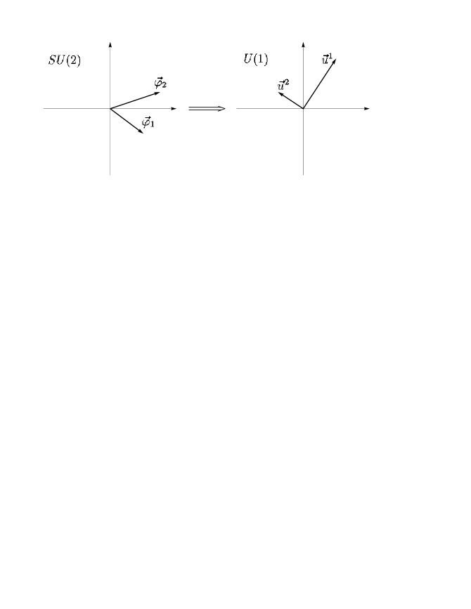
Figure 3: $SU(2)$ and $SO(2)$

To parametrise the special pair $(\vec{\varphi}_{1},\vec{\varphi}_{2})$ note that the numbers $\varphi^{a}_{i}$ form also a pair of $SO(2)$ (Lorentz) orthogonal vectors: $u^{1}=\{\varphi_{1}^{1},\varphi_{2}^{1}\}$ and $u^{2}=\{\varphi_{1}^{2},\varphi_{2}^{2}\}$, so that $\arg u^{2}=\arg u^{1}+\frac{\pi}{2}$. The remaining coordinates $\{f,g,\theta\}$ are defined to be the polar coordinates for $u^{1}$ and $u^{2}$:

$$\begin{array}[]{l}\varphi_{1}^{1}=f\cos\theta\\ \varphi_{2}^{1}=f\sin\theta\end{array}~{}~{}~{}\begin{array}[]{l}\varphi_{1}^{2}=-g\sin\theta\\ \varphi_{2}^{2}=g\cos\theta.\end{array}$$ (43)

As the pair is the special one the ranges for $\{f,g,\theta\}$ are $0\leq\theta<\pi/2$ and $f,g>0$.

To summarize, we have proved that by the $SU(2)$ rotation defined by the Euler-like angles $\gamma_{1}$, $\gamma_{2}$ and $\alpha$ any pair $(\vec{\varphi}_{1},\vec{\varphi}_{2})$ is matched with the special pair which is parametrised by $f,g,\theta$. The special case of an angular momentum parametrisation was proposed in [7].

3.2 Generalized Periodicity

To extend the ranges for the angular variables $\gamma_{i}$ up to $R^{1}$ axis we employ the usual $2\pi$ periodicity conditions for $\gamma_{i}$. As to the $\theta$ angle with $0\leq\theta<\pi/2$ the situation is more subtle.

Let us take a point with $SO(2)$ angle coordinate outside the range: $(f,g,\theta+\frac{\pi}{2},\gamma_{1})$ ($\gamma_{2}$ and $\alpha$ are irrelevant for the subsequent discussion). By means of (33) this set parametrise the pair

$$\varphi_{1,2}=U^{+}(\gamma_{1})\chi_{1,2}U(\gamma_{1}),~{}~{}~{}U(\gamma_{1})=e^{\frac{i}{2}\gamma_{1}\sigma_{3}}$$

where

$$\chi_{1} = -\sigma_{1}f\sin\theta+\sigma_{2}g\cos\theta,$$

$$\chi_{2} = \sigma_{1}f\cos\theta-\sigma_{2}g\sin\theta.$$ (44)

The pair $(\vec{\chi}_{1},\vec{\chi}_{2})$ is $SO(2)$-orthogonal but not special. What are the true coordinates for $\varphi_{1,2}$?

In complex notation (29) these read:

$$\varphi = \left(\begin{array}[]{cc}e^{\frac{i}{2}\gamma_{1}}&0\\ 0&e^{-\frac{i}{2}\gamma_{1}}\end{array}\right)^{+}e^{i(\theta+\frac{\chi}{2})}(\sigma_{1}f+i\sigma_{2}g)\left(\begin{array}[]{cc}e^{\frac{i}{2}\gamma_{1}}&0\\ 0&e^{-\frac{i}{2}\gamma_{1}}\end{array}\right)$$ (49)

$$= e^{i\theta}\left(\begin{array}[]{cc}0&e^{-i(\gamma_{1}-\frac{\chi}{2})}(f+g)\\ e^{i(\gamma_{1}+\frac{\chi}{2})}(f-g)&0\end{array}\right)$$ (52)

$$= e^{i\theta}\left(\begin{array}[]{cc}0&e^{-i(\gamma_{1}-\frac{\chi}{2})}(f+g)\\ e^{i(\gamma_{1}-\frac{\chi}{2})}(g-f)&0\end{array}\right)$$ (55)

Hence, the following points must be identified

$$(f,g,\theta+\frac{\pi}{2},\gamma_{1},\gamma_{2},\alpha)\cong(g,f,\theta,\gamma_{1}-\frac{\pi}{2},\gamma_{2},\alpha).$$ (56)

Below we shall call (56) the generalized periodicity condition in $\theta$.

3.3 $P$ symmetry in $SU(2)\times SO(2)$ Parametrisation

On bosonic degrees of freedom $P$ operator acts as $\vec{\varphi}_{1}\leftrightarrow\vec{\varphi}_{2}$. Here we describe this action in terms of the new coordinates. Let us denote $\vec{\varphi}_{1}^{\prime}=\vec{\varphi}_{2}$, $\vec{\varphi}_{2}^{\prime}=\vec{\varphi}_{1}$, then $P\vec{\varphi}_{i}=\vec{\varphi}_{i}^{\prime}$. We also shall indicate by primes all the objects referred to the pair $(\vec{\varphi}_{1}^{\prime},\vec{\varphi}_{2}^{\prime})$.

By definition one has $\vec{e}~{}^{\prime}_{3}=-\vec{e}_{3}$ and $\vec{e}~{}^{\prime}_{n}=-\vec{e}_{n}$ hence, $\gamma_{2}^{\prime}=-\pi+\gamma_{2}$. After $\gamma_{2}$ rotation $\vec{e}~{}^{\prime}_{3}$ lies in the $(x,y)$ plane with $(\vec{e}~{}^{\prime}_{3})_{z}=-(\vec{e}_{3})_{z}$ and $(\vec{e}~{}^{\prime}_{3})_{y}=(\vec{e}_{3})_{y}$. This yields: $\alpha^{\prime}=-\pi-\alpha$.

Let us compare the results of two first rotations for both the pairs $(\vec{\varphi}_{1},\vec{\varphi}_{2})$ and $(\vec{\varphi}_{1}^{\prime},\vec{\varphi}_{2}^{\prime})$ that lie in $(x,y)$ plane (we still denote the resulting pairs as $(\vec{\varphi}_{1},\vec{\varphi}_{2})$, $(\vec{\varphi}_{1}^{\prime},\vec{\varphi}_{2}^{\prime})$ ). By means of a simple algebra one finds that for $\gamma_{2}^{\prime}$ and $\alpha^{\prime}$ given above:

$$\left(\begin{array}[]{ccc}-1&0&0\\ 0&1&0\\ 0&0&-1\end{array}\right)\times\left(\begin{array}[]{ccc}1&0&0\\ 0&\cos\alpha&\sin\alpha\\ 0&-\sin\alpha&\cos\alpha\end{array}\right)\times\left(\begin{array}[]{ccc}\cos\gamma_{2}&\sin\gamma_{2}&0\\ -\sin\gamma_{2}&\cos\gamma_{2}&0\\ 0&0&1\end{array}\right)=$$

$$\left(\begin{array}[]{ccc}1&0&0\\ 0&\cos\alpha^{\prime}&\sin\alpha^{\prime}\\ 0&-\sin\alpha^{\prime}&\cos\alpha^{\prime}\end{array}\right)\times\left(\begin{array}[]{ccc}\cos\gamma_{2}^{\prime}&\sin\gamma_{2}^{\prime}&0\\ -\sin\gamma_{2}^{\prime}&\cos\gamma_{2}^{\prime}&0\\ 0&0&1\end{array}\right).$$ (57)

i.e. $(\vec{\varphi}_{1}^{\prime},\vec{\varphi}_{2}^{\prime})$ and $(\vec{\varphi}_{1},\vec{\varphi}_{2})$, differs by the rotation on $\pi$ around the $y$-axis. Thus on the $(x,y)$ plane one has:

$$\varphi_{1}^{\prime 1}=-\varphi_{2}^{1} \varphi_{1}^{\prime 2}=\varphi_{2}^{2}$$

$$\varphi_{2}^{\prime 1}=-\varphi_{1}^{1} \varphi_{2}^{\prime 2}=\varphi_{1}^{2}.$$

One can rewrite these relations in polar coordinates (we use complex notation):

$$\mbox{if}~{}~{}~{}~{}~{}~{}~{}~{}~{}~{}\vec{\varphi}_{1}=r_{1}e^{i\mu}, \vec{\varphi}_{2}=r_{2}e^{i\nu}$$ (58)

$$\mbox{then}~{}~{}~{}\vec{\varphi}~{}^{\prime}_{1}=r_{2}e^{i(\pi-\nu)}, \vec{\varphi}~{}^{\prime}_{2}=r_{1}e^{i(\pi-\mu)}.$$ (59)

Let $\gamma_{1}$ be the angle that matches $(\vec{\varphi}_{1},\vec{\varphi}_{2})$ with the special pair $(r_{1}e^{i(\mu+\gamma_{1})},r_{2}e^{i(\nu+\gamma_{1})})$. The pair $(r_{2}e^{-i(\nu+\gamma_{1})},r_{1}e^{-i(\mu+\gamma_{1})})$ is also a special one and

$$(r_{2}e^{-i(\nu+\gamma_{1})},r_{1}e^{-i(\mu+\gamma_{1})})=e^{-i(\gamma_{1}+\pi)}(r_{2}e^{i(\pi-\nu)},r_{1}e^{i(\pi-\mu)})$$

that yields $\gamma_{1}^{\prime}=-\gamma_{1}-\pi=-\gamma_{1}+\pi$ due to periodicity in $\gamma_{1}$. The $f^{\prime},g^{\prime}$ and $\theta^{\prime}$ are easily found to be: $f^{\prime}=f$, $g^{\prime}=g$ and $\theta^{\prime}=\pi/2-\theta$.

Collecting all the pieces together we find the action of $P$ in new coordinates:

$$\gamma_{2} \longrightarrow -\pi+\gamma_{2}$$

$$\alpha \longrightarrow -\pi-\alpha$$

$$\gamma_{1} \longrightarrow \pi-\gamma_{1}$$

$$\theta \longrightarrow \pi/2-\theta$$ (60)

$$f \longrightarrow f$$

$$g \longrightarrow g$$

4 Shrödinger equation in $SU(2)\times SO(2)$ parametrisation

4.1 $N=n$ and Gauss law – an explicit solution

The $SU(2)\times SO(2)$ variables provide the explicit solution for wave function $|\Psi\rangle$ dependence on angular variables.

For $N_{B}$ one deduces

$$N_{B}=-i\frac{\partial}{\partial\theta},$$

i.e. $N_{B}$ eigenfunctions are the plane waves $e^{ik\theta}$. Applying periodicity condition (56) four times we find that wave functions components have to be $2\pi$ periodic so $k$ must be an integer. Thus, from eqs.(27) it follows that $n$ can be integer or half-integer and

$$\mbox{for integer}~{}n:~{}~{}~{}\Psi_{n}\equiv\left(\begin{array}[]{rcc}&\psi_{0}&\\ &\vec{\psi}&\\ &0&\\ &\vec{0}&\end{array}\right)~{}~{}~{}~{}~{}~{}~{}~{}\mbox{for half-integer}~{}n:~{}~{}~{}\Psi_{n}\equiv\left(\begin{array}[]{rcc}&0&\\ &\vec{0}&\\ &\tilde{\psi}_{0}&\\ &\vec{\tilde{\psi}}&\end{array}\right).$$

In the following we shall concentrate on the case of integer $n$, the half-integer case will be sometimes discussed for the sake of completeness.

The components of $SU(2)$ generators $l^{a}$ depend only on ”Euler” angles:

$$l^{1} = -i\left(\cos\gamma_{2}\frac{\partial}{\partial\alpha}+\frac{\sin\gamma_{2}}{\sin\alpha}\left(\frac{\partial}{\partial\gamma_{1}}-\cos\alpha\frac{\partial}{\partial\gamma_{2}}\right)\right),$$ (61)

$$l^{2} = -i\left(\sin\gamma_{2}\frac{\partial}{\partial\alpha}-\frac{\cos\gamma_{2}}{\sin\alpha}\left(\frac{\partial}{\partial\gamma_{1}}-\cos\alpha\frac{\partial}{\partial\gamma_{2}}\right)\right),$$ (62)

$$l^{3} = -i\frac{\partial}{\partial\gamma_{2}},$$ (63)

$$(\vec{l})^{2} = -\frac{\partial^{2}}{\partial\alpha^{2}}-\frac{\cos\alpha}{\sin\alpha}\frac{\partial}{\partial\alpha}-\frac{1}{\sin^{2}\alpha}\left(\frac{\partial^{2}}{\partial\gamma^{2}_{1}}+\frac{\partial^{2}}{\partial\gamma^{2}_{2}}-2\cos\alpha\frac{\partial}{\partial\gamma_{1}}\frac{\partial}{\partial\gamma_{2}}\right).$$ (64)

These expressions coincide with the usual Euler angles parametrisation for $SO(3)$ generators [39] up to some modification of variables.

For $\psi_{0}$ ($\tilde{\psi}_{0}$) eq.(26) shows that $\psi_{0}$ does not depend on $(\gamma_{1},\gamma_{2},\alpha)$ and has the form:

$$\mbox{for integer}~{}n:~{}~{}~{} \psi_{0}= e^{in\theta}F_{0}(f,g)$$

$$\mbox{for half-integer}~{}n:~{}~{}~{} \tilde{\psi}_{0}= e^{i(n-\frac{3}{2})\theta}\tilde{F}_{0}(f,g).$$ (65)

From (63) one finds $\psi^{3}$ ($\tilde{\psi}^{3}$) to depend only on $\alpha$ and $\gamma_{1}$. Thus, taking $\psi^{3}(f,g,\theta,\alpha,\gamma_{1})=\sum F(f,g,\theta)\Phi(\alpha,\gamma_{1})$ from (64) one has:

$$\left(\frac{\partial^{2}}{\partial\alpha^{2}}+\frac{\cos\alpha}{\sin\alpha}\frac{\partial}{\partial\alpha}+\frac{1}{\sin^{2}\alpha}\frac{\partial^{2}}{\partial\gamma^{2}_{1}}\right)\Phi=-2\Phi.$$ (66)

The solutions of (66) are spherical functions $Y_{1,m}$ with $m=0,+1,-1$. Taking for $Y_{1,m}$ the explicit expressions we get:

$$\mbox{for integer}~{}n:~{}~{}~{}~{}~{}~{}\psi^{3} = e^{i(n-1)\theta}\left(F^{0}\cos\alpha+F^{+}\sin\alpha e^{i\gamma_{1}}+F^{-}\sin\alpha e^{-i\gamma_{1}}\right),$$ (67)

$$\mbox{for half-integer}~{}n:~{}~{}\tilde{\psi}^{3} = e^{i(n-1/2)\theta}\left(\tilde{F}^{0}\cos\alpha+\tilde{F}^{+}\sin\alpha e^{i\gamma_{1}}+\tilde{F}^{-}\sin\alpha e^{-i\gamma_{1}}\right)$$ (69)

where the harmonics $F^{0},F^{+},F^{-}$ are functions of $f$ and $g$ only.

We list the remaining components of $\vec{\psi}$ ($\vec{\tilde{\psi}}$) which are restored by acting of $l^{a}$ on $\psi^{3}$ ($\tilde{\psi}^{3}$). It is useful to slightly modify the basis by passing to the eigenvectors of $l^{3}$ ($s^{3}$):

$$|\Psi\rangle = (\psi_{0}+\psi^{-}(\bar{\chi}^{1}+i\bar{\chi}^{2})\bar{\chi}^{3}+\psi^{+}(\bar{\chi}^{1}-i\bar{\chi}^{2})\bar{\chi}^{3}+\psi^{3}\bar{\chi}^{1}\bar{\chi}^{2}$$ (70)

$$+ \tilde{\psi}_{0}+\tilde{\psi}^{-}(\bar{\chi}^{1}+i\bar{\chi}^{2})+\tilde{\psi}^{+}(\bar{\chi}^{1}-i\bar{\chi}^{2})+\tilde{\psi}^{3}\bar{\chi}^{3})|0\rangle.$$

In this basis $\psi^{\pm}$ are achieved by using the raising and lowering operators $l^{\pm}=l^{1}\pm il^{2}$ as

$$\psi^{-}=-\frac{i}{2}l^{-}\psi^{3},~{}~{}~{}~{}~{}\psi^{+}=-\frac{i}{2}l^{+}\psi^{3},$$ (71)

similarly for the tildes. Finally, we have
for integer $n$:

$$\psi^{+} = \frac{1}{2}e^{i(n-1)\theta}e^{i\gamma_{2}}\left(F^{0}\sin\alpha-F^{+}(\cos\alpha+1)e^{i\gamma_{1}}-F^{-}(\cos\alpha-1)e^{-i\gamma_{1}}\right),$$ (72)

$$\psi^{-} = \frac{1}{2}e^{i(n-1)\theta}e^{-i\gamma_{2}}\left(F^{0}\sin\alpha-F^{+}(\cos\alpha-1)e^{i\gamma_{1}}-F^{-}(\cos\alpha+1)e^{-i\gamma_{1}}\right),$$ (73)

for half-integer $n$:

$$\tilde{\psi}^{+} = -\frac{i}{2}e^{i(n-1/2)\theta}e^{i\gamma_{2}}\left(\tilde{F}^{0}\sin\alpha-\tilde{F}^{+}(\cos\alpha+1)e^{i\gamma_{1}}-\tilde{F}^{-}(\cos\alpha-1)e^{-i\gamma_{1}}\right),$$ (74)

$$\tilde{\psi}^{-} = \frac{i}{2}e^{i(n-1/2)\theta}e^{-i\gamma_{2}}\left(\tilde{F}^{0}\sin\alpha-\tilde{F}^{+}(\cos\alpha-1)e^{i\gamma_{1}}-\tilde{F}^{-}(\cos\alpha+1)e^{-i\gamma_{1}}\right).$$ (75)

Further restrictions and symmetry properties of $F$-s come from the generalized $\theta$-periodicity (56). We shall examine the case of integer $n$, half-integer case is similar.

Applying (56) twice we obtain restrictions dependent on $n$:

$$\mbox{even}~{}~{}n,~{}~{}~{}~{}~{}~{}~{}~{}n=2k \Rightarrow F^{0}=0,$$

$$\mbox{odd}~{}~{}n \Rightarrow F_{0}=F^{+}=F^{-}=0.$$

Applying (56) once we get that only the following functions $F$ are consistence with the general periodicity:

$$n=4k:~{}~{}~{}~{} F^{0}=0$$ (76)

$$F_{0}(f,g)=F_{0}(g,f)$$

$$F^{+}(f,g)=F^{+}(g,f)$$

$$F^{-}(f,g)=-F^{-}(g,f),$$

$$n=4k+2: F^{0}=0$$ (77)

$$F_{0}(f,g)=-F_{0}(g,f)$$

$$F^{+}(f,g)=-F^{+}(g,f)$$

$$F^{-}(f,g)=F^{-}(g,f),$$

$$n=4k+1: F_{0}=F^{+}=F^{-}=0$$ (78)

$$F^{0}(f,g)=F^{0}(g,f),$$

$$n=4k+3: F_{0}=F^{+}=F^{-}=0$$ (79)

$$F^{0}(f,g)=-F^{0}(g,f).$$

4.2 Hamiltonian

We deduce the explicit expression for $H_{B}$ in new variables as follows. At first, we calculate the metric tensor $g^{\alpha\beta}$: $\delta^{ab}\delta_{ij}d\phi^{a}_{i}d\phi^{b}_{j}=g^{\alpha\beta}dx^{\alpha}dx^{\beta}$ with $\vec{x}=(f,g,\theta,\gamma_{1},\gamma_{2},\alpha)$. At second, we obtain the Hamiltonian as the Laplace-Beltrami operator for the metric $g^{\alpha\beta}$ plus the potential term

$$\frac{1}{8g_{s}}f^{2}g^{2}.$$

This straightforward but rather tedious calculation was performed with partial use of     ”Maple”. The result is the following:

$$H_{B} = -g_{s}\left\{\Delta+D-\frac{A}{a^{2}}(\vec{l})^{2}+\frac{1}{(b)^{2}}\left(c\frac{\partial^{2}}{\partial\theta^{2}}+4a\frac{\partial}{\partial\gamma_{1}}\frac{\partial}{\partial\theta}\right)-\frac{b\sin 2\gamma_{1}}{a^{2}\sin\alpha}\left(\cos\alpha\frac{\partial}{\partial\gamma_{1}}-\frac{\partial}{\partial\gamma_{2}}\right)\frac{\partial}{\partial\alpha}\right.$$ (80)

$$+ \frac{b\cos 2\gamma_{1}}{a^{2}}\frac{\partial^{2}}{\partial\alpha^{2}}-\frac{B}{a^{2}b^{2}}\frac{\partial^{2}}{\partial\gamma_{1}^{2}}\left.+\frac{b\sin 2\gamma_{1}}{2a^{2}\sin^{2}\alpha}\left((1+\cos^{2}\alpha)\frac{\partial}{\partial\gamma_{1}}-2\cos\alpha\frac{\partial}{\partial\gamma_{2}}\right)\right\}+\frac{1}{8g_{s}}a^{2},$$

here $\Delta$ is Laplacian in $f$, $g$ and:

$$D=\frac{1}{J}\left(\frac{\partial J}{\partial f}\frac{\partial}{\partial f}+\frac{\partial J}{\partial g}\frac{\partial}{\partial g}\right),$$

$$a=fg,~{}~{}b=f^{2}-g^{2},~{}~{}c=f^{2}+g^{2},~{}~{}J=ab,$$

$$A=f^{2}\sin^{2}\gamma_{1}+g^{2}\cos^{2}\gamma_{1},$$

$$B=f^{6}\sin^{2}\gamma_{1}-3f^{4}g^{2}\sin^{2}\gamma_{1}-3f^{2}g^{4}\cos^{2}\gamma_{1}+g^{6}\cos^{2}\gamma_{1}.$$

Note that there are terms with the first order derivatives $\frac{\partial}{\partial f}$ and $\frac{\partial}{\partial g}$ collected in $D$. Although the coefficients for these terms are functions of $f$, $g$ only, these terms are absent in the usual quantization of the two-dimensional toy model [1], as in the pure bosonic case as in the fermionic one. These first order derivatives in couple with the zoo of angular dependent terms in (80) radically modify the potential.

4.3 Shrödinger Equation for Harmonics

Now we substitute the harmonic expansion for the wave function $\Psi_{n}$ into the system (31) with the explicit Hamiltonian $H_{B}$ given in (80). The result is:

for $n$ - odd (only $F^{0}\neq 0$) we get one PDE in $f$ and $g$

$$-g_{s}\left\{\Delta+D-(n-1)^{2}\frac{c}{b^{2}}-\frac{c}{a^{2}}\right\}F^{0}+\frac{a^{2}}{8g_{s}}F^{0}=EF^{0},$$ (81)

for $n$ - even we get a system of three PDE in $f$ and $g$

$$-g_{s}\left\{\Delta+D-n^{2}\frac{c}{b^{2}}\right\}F_{0}+\frac{1}{8g_{s}}a^{2}F_{0}-\frac{f+g}{\sqrt{2}}F^{+}+\frac{f-g}{\sqrt{2}}F^{-}=EF_{0}$$ (82)

$$-g_{s}\left\{\left(\Delta+D-(n-1)^{2}\frac{c}{b^{2}}-(n-1)\frac{4a}{b^{2}}-\frac{(f^{4}+g^{4})c}{2a^{2}b^{2}}\right)\right.F^{+}\left.-\frac{b}{2a^{2}}F^{-}\right\}$$

$$\hskip 199.16928pt+\frac{a^{2}}{8g_{s}}F^{+}-F_{0}\frac{f+g}{2\sqrt{2}}=EF^{+}$$ (83)

$$-g_{s}\left\{\left(\Delta+D-(n-1)^{2}\frac{c}{b^{2}}+(n-1)\frac{4a}{b^{2}}-\frac{(f^{4}+g^{4})c}{2a^{2}b^{2}}\right)F^{-}-\frac{b}{2a^{2}}F^{+}\right\}$$

$$\hskip 199.16928pt+\frac{a^{2}}{8g_{s}}F^{-}+F_{0}\frac{f-g}{2\sqrt{2}}=EF^{-}.$$ (84)

5 The Spectrum

Remind, that for any $E\neq 0$ eigenfunctions are combined into the quartets $V_{E,n_{q}}$ with quantum numbers $n_{q},n_{q}-1/2,-n_{q}+2,-n_{q}+3/2$. To examine the spectrum it is sufficient to search for any one of these four functions constrained by the additional constraints coming from supercharges $Q$ and $\bar{Q}$. Next we search for differential equations for these constraints.

5.1 Supercharges

In the basis (22) the supercharges $Q$ and $\bar{Q}$ take the form of anti-block-diagonal matrices:

$$Q=\left(\begin{array}[]{ll}0&Q_{+}^{*}\\ Q_{-}&0\end{array}\right)~{}~{}~{}~{}~{}~{}~{}~{}\bar{Q}=\left(\begin{array}[]{ll}0&Q_{-}^{*}\\ Q_{+}&0\end{array}\right),$$

where asterisk stands for Hermitian conjugation.

The $4\times 4$ blocks are calculated to give:

$$Q_{-}=\frac{-1}{\sqrt{2}}\left(\begin{array}[]{cccc}0&\sqrt{g_{s}}\pi^{1}&\sqrt{g_{s}}\pi^{2}&\sqrt{g_{s}}\pi^{3}\\ \sqrt{g_{s}}\pi^{1}&0&\frac{-i}{\sqrt{g_{s}}}{\omega}^{3}&\frac{i}{\sqrt{g_{s}}}{\omega}^{2}\\ \sqrt{g_{s}}\pi^{2}&\frac{i}{\sqrt{g_{s}}}{\omega}^{3}&0&\frac{-i}{\sqrt{g_{s}}}{\omega}^{1}\\ \sqrt{g_{s}}\pi^{3}&\frac{-i}{\sqrt{g_{s}}}{\omega}^{2}&\frac{i}{\sqrt{g_{s}}}{\omega}^{1}&0\end{array}\right),$$

$$Q_{+}=\frac{-1}{\sqrt{2}}\left(\begin{array}[]{cccc}0&\frac{i}{\sqrt{g_{s}}}\omega^{1}&\frac{i}{\sqrt{g_{s}}}\omega^{2}&\frac{i}{\sqrt{g_{s}}}\omega^{3}\\ \frac{i}{\sqrt{g_{s}}}\omega^{1}&0&\sqrt{g_{s}}\bar{\pi}^{3}&-\sqrt{g_{s}}\bar{\pi}^{2}\\ \frac{i}{\sqrt{g_{s}}}\omega^{2}&-\sqrt{g_{s}}\bar{\pi}^{3}&0&\sqrt{g_{s}}\bar{\pi}^{1}\\ \frac{i}{\sqrt{g_{s}}}\omega^{3}&\sqrt{g_{s}}\bar{\pi}^{2}&-\sqrt{g_{s}}\bar{\pi}^{1}&0\\ \end{array}\right);$$

here we used the complex notation (29), $\vec{\pi}=\vec{\pi}_{1}-i\vec{\pi}_{2}$ and $\vec{\omega}=\vec{\varphi_{1}}\times\vec{\varphi_{2}}$.

For integer $n$ (see eq.(4.1)):

$$\Psi\equiv\left(\begin{array}[]{rcc}&\psi_{0}&\\ &\vec{\psi}&\\ &0&\\ &\vec{0}&\end{array}\right)~{}~{}~{}$$

and equations $Q\Psi=0$, $\bar{Q}\Psi=0$ are reduced to

$$Q_{-}\left(\begin{array}[]{c}\psi_{0}\\ \vec{\psi}\end{array}\right) {\displaystyle=\frac{-1}{\sqrt{2}}}\left(\begin{array}[]{l}\sqrt{g_{s}}(\vec{\pi}\vec{\psi})\\ \sqrt{g_{s}}\vec{\pi}\psi_{0}+\frac{i}{\sqrt{g_{s}}}\vec{\omega}\times\vec{\psi}\end{array}\right) =\frac{-1}{\sqrt{2}}\left(\begin{array}[]{l}\sqrt{g_{s}}\mbox{div}\vec{\psi}\\ \sqrt{g_{s}}\mbox{grad}\psi_{0}+\frac{i}{\sqrt{g_{s}}}\vec{\omega}\times\vec{\psi}\end{array}\right)=0.$$ (91)

$$Q_{+}\left(\begin{array}[]{c}\psi_{0}\\ \vec{\psi}\end{array}\right) {\displaystyle=\frac{-1}{\sqrt{2}}}\left(\begin{array}[]{l}\frac{i}{\sqrt{g_{s}}}(\vec{\omega}\vec{\psi})\\ \frac{i}{\sqrt{g_{s}}}\vec{\omega}\psi_{0}-\sqrt{g_{s}}\vec{\bar{\pi}}\times\vec{\psi}\end{array}\right) =\frac{-1}{\sqrt{2}}\left(\begin{array}[]{l}\frac{i}{\sqrt{g_{s}}}(\vec{\omega}\vec{\psi})\\ \frac{i}{\sqrt{g_{s}}}\vec{\omega}\psi_{0}-\sqrt{g_{s}}\bar{\mbox{rot}}\vec{\psi}\end{array}\right)=0.$$ (98)

5.2 Supercharges in $SU(2)\times SO(2)$ Parametrisation

At first we do not specify the parity of $n$ and employ the harmonics expansion (eqs. (67), (72), (73)) for $\Psi_{n}$. The nondifferential terms in (91), (98) can be easily calculated to give:

$$\vec{\omega}=\frac{fg}{2}\vec{v},$$ (99)

$$(\vec{\omega}\vec{\psi})=e^{i(n-1)\theta}\frac{fg}{2}F^{0},$$ (100)

$$\vec{\omega}\times\vec{\psi}=-e^{i(n-1)\theta}\frac{fg}{2}\left(e^{i\gamma_{1}}F^{+}\vec{u}+e^{-i\gamma_{1}}F^{-}\vec{w}\right)$$ (101)

where we have introduced three vectors:

$$\vec{u} = \{\cos\gamma_{2}+i\cos\alpha\sin\gamma_{2},~{}~{}\sin\gamma_{2}-i\cos\alpha\cos\gamma_{2},~{}~{}-i\sin\alpha\},$$

$$\vec{v} = \{\sin\alpha\sin\gamma_{2},~{}~{}-\sin\alpha\cos\gamma_{2},~{}~{}\cos\alpha\},$$

$$\vec{w} = \{\cos\gamma_{2}-i\cos\alpha\sin\gamma_{2},~{}~{}\sin\gamma_{2}+i\cos\alpha\cos\gamma_{2},~{}~{}i\sin\alpha\}.$$ (102)

The explicit expressions for $\vec{\pi}$ $\vec{\bar{\pi}}$, are too bulky and are listed in the Appendix. Here we quote the results deduced by means of the computer calculations:

$$\vec{\pi}\psi_{0}=\frac{1}{i\sqrt{2}}e^{i(n-1)\theta}\left(e^{i\gamma_{1}}R^{+}_{n}F_{0}\vec{u}+e^{-i\gamma_{1}}R^{-}_{n}F_{0}\vec{w}\right),$$ (103)

$$\vec{\pi}\vec{\psi}=\sqrt{2}e^{i(n-2)\theta}\left[\left(R^{-}_{n}-\frac{(f-g)}{fg}\right)F^{+}\right.\left.-\left(R^{+}_{n}+\frac{(f+g)}{fg}\right)F^{-}\right],$$ (104)

$$\vec{\bar{\pi}}\times\vec{\psi}=-i2\sqrt{2}e^{in\theta}\frac{1}{fg}\left(R^{+}_{2-n}F^{+}+R^{-}_{2-n}F^{-}\right)\vec{\omega}+LF^{0},$$ (105)

where

$$R^{+}_{n}=\left(\frac{\partial}{\partial_{f}}+\frac{\partial}{\partial_{g}}+\frac{n}{f+g}\right),~{}~{}~{}R^{-}_{n}=\left(\frac{\partial}{\partial_{f}}-\frac{\partial}{\partial_{g}}+\frac{n}{f-g}\right)$$ (106)

and$L$ is an irrelevant differential operator

Remind, that the harmonics content of the wave function $\Psi_{n}$ differs with respect to the parity of $n$:

$$\mbox{for odd}~{}~{}n: F_{0}=F^{+}=F^{-}=0$$

$$\mbox{for even}~{}~{}n: F^{0}=0$$

At the same time it is seen from eqs. (101), (104) that all the terms in eq.(91) for $Q_{-}$ are expressed solely in terms of $F^{\pm}$ and $F_{0}$. Hence, for

$$\mbox{\bf odd}~{}~{}n:~{}~{}~{}~{}~{}~{}Q\Psi_{En}\equiv 0.$$ (107)

On the other hand, it is known that $H\Psi_{n}=E\Psi_{n}$ and $Q\Psi_{n}=0$ implies $\bar{Q}\Psi_{n}\neq 0$, i.e. for

$$\mbox{\bf odd}~{}~{}n:~{}~{}~{}~{}~{}~{}\bar{Q}\Psi_{En}\neq 0.$$ (108)

The case of even $n$ is more involved. By using the above formulae we get

$$\begin{array}[]{rcl}\mbox{\bf even }~{}n:~{}\bar{Q}\Psi=0&\rightarrow&\sqrt{2g_{s}}\left(\displaystyle R^{+}_{2-n}F^{+}+R^{-}_{2-n}F^{-}\right)\displaystyle+\frac{fg}{2\sqrt{g_{s}}}F_{0}=0\end{array}$$ (109)

and

$$\begin{array}[]{rcl}\mbox{\bf even}~{}n:~{}Q\Psi=0&\rightarrow&\left\{\begin{array}[]{l}\sqrt{2g_{s}}R^{+}_{n}F_{0}\displaystyle+\frac{fg}{\sqrt{g_{s}}}F^{+}=0\\ \\ \sqrt{2g_{s}}R^{-}_{n}F_{0}\displaystyle+\frac{fg}{\sqrt{g_{s}}}F^{-}=0\\ \\ \left(R^{-}_{n}-\displaystyle\frac{(f-g)}{fg}\right)F^{+}-\left(\displaystyle R^{+}_{n}-\frac{(f+g)}{fg}\right)F^{-}=0.\\ \end{array}\right.\end{array}$$ (110)

One can express $F^{+}$ and $F^{-}$ from the first and the second equations respectively. The third equation of the system above is nothing but the consistency condition for the first and the second ones.

Now we are in position to examine the restrictions on $V_{E,n_{q}}$ coming from $Q\Psi_{n}=0$ and $\bar{Q}\Psi_{n}=0$. As it was shown above $n$ can be integer or half-integer. We start with the case of integer $n_{q}$. (We omit the subindex $q$ below). The content of $V_{En}$ is the following: $\Psi_{n}$, $\Psi_{n-\frac{1}{2}}$, $\Psi_{-n+2}$ and $\Psi_{-n+\frac{3}{2}}$ with $\bar{Q}\Psi_{n}=0$ and $\bar{Q}\Psi_{-n+2}=0$. Both $n$ and $-n+2$ have the same parity so according to (108) odd $n$ are forbidden. For $n$ even the constraint $\bar{Q}\Psi_{n}=0$ results in PDE (109). We shall examine this case in Sec. 5.4.

Next we turn to a half-integer $n=n^{\prime}+\frac{1}{2}$. $V_{En^{\prime}+\frac{1}{2}}$ is spanned by $\Psi_{n^{\prime}+\frac{1}{2}}$, $\Psi_{n^{\prime}}$, $\Psi_{-n^{\prime}+\frac{3}{2}}$ and $\Psi_{-n^{\prime}+1}$ with $Q\Psi_{n^{\prime}}=0$, $Q\Psi_{-n^{\prime}+1}=0$. This time one of two numbers either $n^{\prime}$ or $-n^{\prime}+1$ will be odd. Let, for instance, $n^{\prime}$ to be odd. As follows from (107) $Q\Psi_{n^{\prime}}=0$ and the only equation to be solved is the Shrödinger equation (81). It will be examined in the next section.

5.3 Half-integer $n_{q}$

In this section we examine the solution of eq. (81)

$$-g_{s}\left(\Delta+D-\frac{g^{2}+f^{2}}{g^{2}f^{2}}-(n-1)^{2}\frac{g^{2}+f^{2}}{(f^{2}-g^{2})^{2}}\right)F^{0}+\frac{f^{2}g^{2}}{8g_{s}}F^{0}=EF^{0}$$

by using the Born-Oppenheimer method in the region $f\gg g$, as it is adopted in current literature. This procedure yields an approximate formulae for the spectrum and wave function. Note, that in the current variables $\|\Psi\|$ is proportional to $\int\bar{F^{0}}F^{0}Jdfdg$.

To eliminate the first derivatives term $D$ we search for the wave function in the form

$$F^{0}=\frac{1}{\sqrt{J}}\varphi^{0}$$

that yields the equation

$$-g_{s}\left(\Delta+\frac{1}{4}\frac{(f^{2}+g^{2})^{3}}{f^{2}g^{2}(f^{2}-g^{2})^{2}}-\frac{g^{2}+f^{2}}{g^{2}f^{2}}-(n-1)^{2}\frac{g^{2}+f^{2}}{(f^{2}-g^{2})^{2}}\right)\varphi^{0}+\frac{f^{2}g^{2}}{8g_{s}}\varphi^{0}=E\varphi^{0}$$ (111)

and

$$\|\Psi\|=C\int\bar{\varphi}^{0}\varphi^{0}dfdg.$$

We start with introducing an extra parameter $a$ as follows: $f\to f/a^{2}$ and $g\to ag$ and expanding over the powers of $a$. Separating the variables as $\varphi^{0}=\psi_{m}(g|f)\chi_{k}(f)$ we get the leading term as

$$\left(-\frac{\partial^{2}}{\partial g^{2}}+\frac{3}{4}\frac{1}{g^{2}}+b^{2}g^{2}\right)\psi_{m}=\varepsilon_{m}\psi_{m}$$

where $b=\frac{f}{2\sqrt{2}g_{s}}$.

The discrete spectrum is given by $\varepsilon_{m}=4b(m+1)$ where $m=0,1,2,\dots$ and $\psi_{m}$ is expressed in terms of Laguerre polynomials

$$\psi_{m}=(-1)^{m}\frac{1}{\sqrt{g}}bg^{2}e^{-\frac{1}{2}bg^{2}}L_{m}^{1}(bg^{2}).$$

The next to leading term in the $a$-expansion yields the equation for $\chi$ (we omit the index $k$)

$$(-\frac{\partial^{2}}{\partial f^{2}}+4\frac{f}{2\sqrt{2}g_{s}}(m+1))\chi=E\chi$$

where we temporary suppressed the term $1/f^{2}$. The change of variables $f=x+E\frac{\sqrt{2}g_{s}}{2(m+1)}$ yields an equation for Airy function

$$\left(\frac{\partial^{2}}{\partial x^{2}}-\frac{\sqrt{2}(m+1)}{g_{s}}x\right)\chi=0.$$

The solution in terms of $y=(\frac{\sqrt{2}(m+1)}{g_{s}})^{1/3}x$ is

$$\chi=\left\{\begin{array}[]{lll}\sqrt{\frac{y}{3\pi}}K_{1/3}\left(\frac{2}{3}y^{3/2}\right)&~{}\mbox{for}{}&y>0\\ \frac{\sqrt{\pi|y|}}{3}\left(J_{-1/3}\left(\frac{2}{3}|y|^{3/2}\right)+J_{1/3}\left(\frac{2}{3}|y|^{3/2}\right)\right)&~{}\mbox{for}{}&y<0.\\ \end{array}\right.$$

Imposing a boundary condition $\chi(0)=0$ we get

$$J_{-1/3}(\rho_{k})+J_{1/3}(\rho_{k})=0$$

where

$$\rho_{k}=\frac{\sqrt{2}}{3}\frac{g_{s}}{m+1}E^{3/2}.$$

By using

$$J_{\nu}(\rho)+J_{-\nu}(\rho)=2\cos\frac{\pi\nu}{2}\left(J_{\nu}(\rho)\cos\frac{\pi\nu}{2}-N_{\nu}(\rho)\sin\frac{\pi\nu}{2}\right)$$

and asymptotic of $J(\rho)$ and $N(\rho)$ for large $\rho$

$$J_{\nu}(\rho)\approx\sqrt{\frac{2}{\pi\rho}}\cos\left(\rho-\frac{\pi}{2}\nu-\frac{\pi}{4}\right)$$

$$N_{\nu}(\rho)\approx\sqrt{\frac{2}{\pi\rho}}\sin\left(\rho-\frac{\pi}{2}\nu-\frac{\pi}{4}\right)$$

we get

$$\rho_{k}=\pi k+\frac{3}{4}\pi,~{}~{}~{}k=0,1,2,\dots$$

Thus, the result is

$$E_{m,k}=\left(\pi\frac{3}{\sqrt{2}}\frac{(m+1)(k+\frac{3}{4})}{g_{s}}\right)^{2/3}$$

and

$$\varphi_{m,k}\!\sim\!c_{m,k}fg^{3/2}\xi e^{-\frac{\alpha}{2}fg^{2}}L_{m}^{1}(\alpha fg^{2})\times\left\{\begin{array}[]{ll}\frac{\sqrt{3}}{\pi}K_{1/3}\!\left(\frac{2}{3}a^{1/2}\xi^{3}\right),&f>\frac{1}{a}E_{m,k}\\ J_{1/3}\!\left(\frac{2}{3}a^{1/2}\xi^{3}\right)+J_{-1/3}\!\left(\frac{2}{3}a^{1/2}\xi^{3}\right),&f<\frac{1}{a}E_{m,k}\end{array}\right.$$ (112)

where

$$\alpha=\frac{1}{2\sqrt{2}g_{s}},~{}~{}~{}a=\frac{\sqrt{2}(m+1)}{g_{s}},~{}~{}~{}\xi=\left|f-\frac{1}{a}E_{m,k}\right|^{1/2}$$

The first correction to the energy is given by

$$\Delta E=\frac{\int\bar{\chi}V\chi df}{\int\bar{\chi}\chi df}.$$

In our case $V=\frac{(n-1)^{2}-1/4}{f^{2}}$ and the direct calculation gives

$$E=\left(\frac{3\pi}{\sqrt{2}}\right)^{2/3}\left(\frac{(m+1)(k+\frac{3}{4})}{g_{s}}\right)^{2/3}\left(1+\frac{4}{3}\frac{(n-1)^{2}-\frac{1}{4}}{(k+\frac{3}{4})^{2}}\right).$$

5.4 Even $n_{q}$ and continuous spectrum

Here we apply the Born-Oppenheimer method in the region $f\gg g$ to the system (82) - (84). Our aim is to employ the toy-model-like ansatz for the wave function and justify the appearance of the continuous spectrum [11].

For $f\gg g$ the leading part in the system (82) - (84) reads

$$-(\Delta+D)\tilde{F}_{0}+\frac{1}{8g^{2}_{s}}a^{2}\tilde{F}_{0}-\frac{f}{2g_{s}}F^{+}+\frac{f}{2g_{s}}F^{-}=E\tilde{F}_{0}$$ (113)

$$-(\Delta+D-\frac{1}{2g^{2}})F^{+}+\frac{a^{2}}{8g^{2}_{s}}F^{+}+\frac{1}{2g^{2}}F^{-}-\frac{f}{2g_{s}}\tilde{F}_{0}=EF^{+}$$ (114)

$$-(\Delta+D-\frac{1}{2g^{2}})F^{-}+\frac{a^{2}}{8g^{2}_{s}}F^{-}+\frac{1}{2g^{2}}F^{+}+\frac{f}{2g_{s}}\tilde{F}_{0}=EF^{-}$$ (115)

where we rescaled $F_{0}=\sqrt{2}\tilde{F}_{0}$.

Taking $F^{-}=-F^{+}$ we find that (114) and (115) coincide. The reduced system reads:

$$-(\Delta+D)\tilde{F}_{0}+\frac{1}{8g^{2}_{s}}a^{2}\tilde{F}_{0}-\frac{f}{g_{s}}\tilde{F}_{0}=E\tilde{F}_{0}$$ (116)

$$-(\Delta+D)F^{+}+\frac{a^{2}}{8g^{2}_{s}}F^{-}\frac{f}{2g_{s}A}\tilde{F}_{0}=EF^{+}.$$ (117)

It is obvious that (116) and (117) will coincide as well if one put $F^{+}=\frac{1}{\sqrt{2}}\tilde{F}_{0}$.

In the asymptotic region the rescaling yields $D\to 1/(4g^{2})$ and we are left with the equation

$$-(\Delta+\frac{1}{4g^{2}})\tilde{F}_{0}+\frac{1}{8g^{2}_{s}}f^{2}g^{2}\tilde{F}_{0}-\frac{f}{\sqrt{2}g_{s}}\tilde{F}_{0}=E\tilde{F}_{0}$$

Recall, that equation

$$-(\frac{\partial}{\partial g^{2}}+\frac{1}{4g^{2}})\psi_{m}+\frac{1}{8g^{2}_{s}}f^{2}g^{2}\psi_{m}=\varepsilon_{m}\psi_{m}$$

has normalisable solutions for $\varepsilon_{m}=\frac{\sqrt{2}f}{g_{s}}(m+1/2)$, where $1/2$ is very important (not $1$ !).

The next step is to solve the equation

$$-(\frac{\partial}{\partial f^{2}}+O(\sim 1/f^{2}))\chi=E\chi.$$

We confirm that for $m=0$ the linear term from the ”energy” $\varepsilon_{m}$ is fully cancelled by the linear potential $\frac{f}{\sqrt{2}g_{s}}$ thus producing the continuous spectrum.

6 Discussion and Conclusion

The results obtained in Section 5 are collected in the table presented in Fig.3. States from the quartets are situated along the horizontal lines. Eigenvalues of $N$ for the states in a quartet $n_{q}$ are $n_{q},n_{q}-1/2$ and $-n_{q}+2,-n_{g}+3/2$. Each item of the quartet can be obtained from any other one by the action of supercharges or the permutation operator $P$. Our results show that odd $n_{q}$ are forbidden, for even $n_{q}$ the spectrum has a continuous part as well as a discrete one, meanwhile for half-integer $n_{q}$ the spectrum is purely discrete.

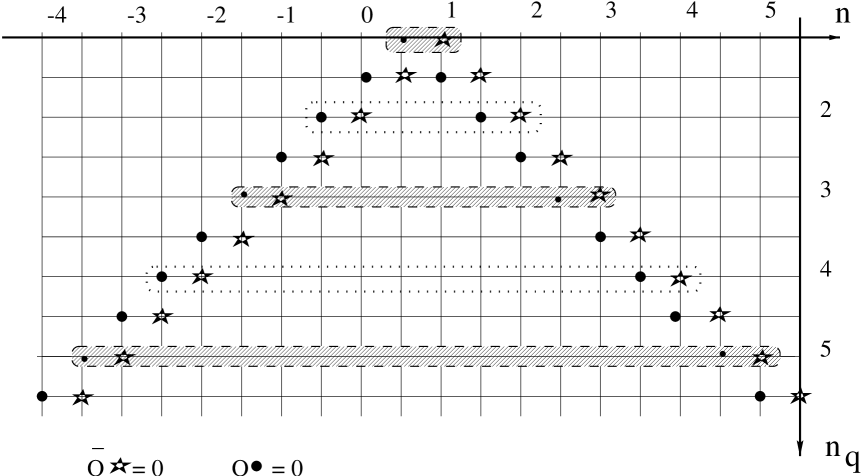
Figure 4: Structure of the spectrum: stars correspond to $\bar{Q}\Psi=0,~{}~{}$filled circles correspond to $Q\Psi=0$; domains bounded by dots correspond to the presence of the continuous spectrum; shared domains correspond to excluding values of $n$ and $n_{q}$. Quartets are located along the horizontal lines.

Table 3 demonstrates that there is a possibility to put a superselection rule to exclude the presence of the continuous spectrum. Namely, taking any state from quartet with half-integer $n_{q}$ one gets with guarantee the state of discrete spectrum. One can also specify the purely discrete sector by using the supercharges, i.e. the states with integer $n$ satisfy the constraint $Q\Psi_{n}=0$, meanwhile states with half-integer $n$ satisfy $\bar{Q}\Psi_{n}=0$.

Besides the continuous spectrum $SU(2)\times SO(2)$ matrix supersymmetric quantum mechanics possesses one more distinguish feature as compared with the bosonic counterpart. This concerns the behaviour of the wave functions in half-integer $n_{q}$ sector, where spectrum is purely discrete. The expression (112) for the wave function illuminates this difference. It is not a difficult task to realize that in the pure bosonic case the maximum of the wave function appears at the minimum of the classical potential $(fg)^{2}$, i.e. at the bottom of the valley $f=0$ as it should be by the semiclassical reasons. For the supersymmetric case the picture is quite different, the classical equilibrium line have nothing to do with the maximum of the wave function (112), this time the wave function tends to zero as $f\to 0$. The origin of this transformation is the reflecting wall like $\frac{1}{f^{2}}$ created by the activation of the $SU(2)$ angular degrees of freedom for the triplet $(l=1)$ solution.

Let us note that we have obtained only the asymptotic formula for spectrum. Numeric investigations (see [40] and references therein) allow to trust the asymptotic formula. It would be interesting to perform numerical calculations also in our case. It would be also interesting to study $\alpha^{\prime}$-corrections [38] to the spectrum.

It was argued [36] that the holographic feature of the matrix theory can be related with the repulsive feature of energy eigenvalues in the quantum chaotic system. Relation between chaos and holography has been discussed recently in [41]. Quantum chaos in supersymmetric matrix quantum mechanics will be a subject of future investigationss.

7 Appendix

Derivatives in new coordinates are

$$\frac{\partial}{\partial\varphi^{+}} = \frac{\sqrt{2}}{4}e^{-i(\theta+\gamma_{2})}\left(\frac{\sin\alpha(f\cos\gamma_{1}+ig\sin\gamma_{1})}{fg}\frac{\partial}{\partial\alpha}+\frac{(f\sin\gamma_{1}-ig\cos\gamma_{1})}{fg}\frac{\partial}{\partial\gamma_{2}}-\right.$$ (118)

$$\frac{(f^{2}g\sin\gamma_{1}+f^{3}\cos\alpha\sin\gamma_{1}+ig^{3}\cos\alpha\cos\gamma_{1}+ifg^{2}\cos\gamma_{1})}{(fg(f^{2}-g^{2}))}\frac{\partial}{\partial\gamma_{1}}-$$

$$\frac{(g\sin\gamma_{1}+f\cos\alpha\sin\gamma_{1}+if\cos\gamma_{1}+ig\cos\gamma_{1}\cos\alpha)}{f^{2}-g^{2}}\frac{\partial}{\partial\theta}-$$

$$\left.(i\cos\alpha\sin\gamma_{1}-\cos\gamma_{1})\frac{\partial}{\partial f}-(\cos\alpha\cos\gamma_{1}-i\sin\gamma_{1})\frac{\partial}{\partial g}\right)$$

$$\frac{\partial}{\partial\varphi^{-}} = -\frac{\sqrt{2}}{4}e^{-i(\theta-\gamma_{2})}\left(\frac{\sin\alpha(f\cos\gamma_{1}+ig\sin\gamma_{1})}{fg}\frac{\partial}{\partial\alpha}+\frac{(f\sin\gamma_{1}-ig\cos\gamma_{1})}{fg}\frac{\partial}{\partial\gamma_{2}}-\right.$$ (119)

$$\frac{(-f^{2}g\sin\gamma_{1}+f^{3}\cos\alpha\sin\gamma_{1}+ig^{3}\cos\alpha\cos\gamma_{1}-ifg^{2}\cos\gamma_{1})}{(fg(f^{2}-g^{2}))}\frac{\partial}{\partial\gamma_{1}}+$$

$$\frac{(g\sin\gamma_{1}-f\cos\alpha\sin\gamma_{1}+if\cos\gamma_{1}-ig\cos\gamma_{1}\cos\alpha)}{f^{2}-g^{2}}\frac{\partial}{\partial\theta}-$$

$$\left.(i\cos\alpha\sin\gamma_{1}+\cos\gamma_{1})\frac{\partial}{\partial f}-(\cos\alpha\cos\gamma_{1}+i\sin\gamma_{1})\frac{\partial}{\partial g}\right)$$

$$\frac{\partial}{\partial\bar{\varphi}^{+}} = -\frac{\sqrt{2}}{4}e^{i(\theta-\gamma_{2})}\left(\frac{\sin\alpha(f\cos\gamma_{1}-ig\sin\gamma_{1})}{fg}\frac{\partial}{\partial\alpha}+\frac{(f\sin\gamma_{1}+ig\cos\gamma_{1})}{fg}\frac{\partial}{\partial\gamma_{2}}-\right.$$ (120)

$$\frac{(-f^{2}g\sin\gamma_{1}+f^{3}\cos\alpha\sin\gamma_{1}-ig^{3}\cos\alpha\cos\gamma_{1}+ifg^{2}\cos\gamma_{1})}{(fg(f^{2}-g^{2}))}\frac{\partial}{\partial\gamma_{1}}-$$

$$\frac{(-g\sin\gamma_{1}+f\cos\alpha\sin\gamma_{1}+if\cos\gamma_{1}-ig\cos\gamma_{1}\cos\alpha)}{f^{2}-g^{2}}\frac{\partial}{\partial\theta}+$$

$$\left.(i\cos\alpha\sin\gamma_{1}-\cos\gamma_{1})\frac{\partial}{\partial f}+(-\cos\alpha\cos\gamma_{1}+i\sin\gamma_{1})\frac{\partial}{\partial g}\right)$$

$$\frac{\partial}{\partial\bar{\varphi}^{-}} = \frac{\sqrt{2}}{4}e^{i(\theta+\gamma_{2})}\left(\frac{\sin\alpha(f\cos\gamma_{1}-ig\sin\gamma_{1})}{fg}\frac{\partial}{\partial\alpha}+\frac{(f\sin\gamma_{1}+ig\cos\gamma_{1})}{fg}\frac{\partial}{\partial\gamma_{2}}+\right.$$ (121)

$$\frac{(-f^{2}g\sin\gamma_{1}-f^{3}\cos\alpha\sin\gamma_{1}+ig^{3}\cos\alpha\cos\gamma_{1}+ifg^{2}\cos\gamma_{1})}{(fg(f^{2}-g^{2}))}\frac{\partial}{\partial\gamma_{1}}-$$

$$\frac{(g\sin\gamma_{1}+f\cos\alpha\sin\gamma_{1}-if\cos\gamma_{1}-ig\cos\gamma_{1}\cos\alpha)}{f^{2}-g^{2}}\frac{\partial}{\partial\theta}+$$

$$\left.(i\cos\alpha\sin\gamma_{1}+\cos\gamma_{1})\frac{\partial}{\partial f}-(\cos\alpha\cos\gamma_{1}+i\sin\gamma_{1})\frac{\partial}{\partial g}\right)$$

$$\frac{\partial}{\partial\varphi^{3}} = -\frac{\sqrt{2}}{2}e^{-i\theta}\left(\frac{\cos\alpha(if\cos\gamma_{1}-g\sin\gamma_{1})}{fg}\frac{\partial}{\partial\alpha}+\frac{\cos\alpha(if\sin\gamma_{1}+g\cos\gamma_{1})}{fg\sin\alpha}\frac{\partial}{\partial\gamma_{2}}-\right.$$ (122)

$$\frac{(f^{2}g\cos\gamma_{1}+if^{3}\cos^{2}\alpha\sin\gamma_{1}-g^{3}\cos^{2}\alpha\cos\gamma_{1}-ifg^{2}\sin\gamma_{1})}{(fg\sin\alpha(f^{2}-g^{2}))}\frac{\partial}{\partial\gamma_{1}}+$$

$$\left.\frac{\sin\alpha(-g\cos\gamma_{1}+if\sin\gamma_{1})}{f^{2}-g^{2}}\frac{\partial}{\partial\theta}-\sin\alpha\sin\gamma_{1}\frac{\partial}{\partial f}+\sin\alpha\cos\gamma_{1}\frac{\partial}{\partial g}\right)$$

$$\frac{\partial}{\partial\bar{\varphi}^{3}} = \frac{\sqrt{2}}{2}e^{i\theta}\left(\frac{\cos\alpha(if\cos\gamma_{1}+g\sin\gamma_{1})}{fg}\frac{\partial}{\partial\alpha}+\frac{\cos\alpha(if\sin\gamma_{1}-g\cos\gamma_{1})}{fg\sin\alpha}\frac{\partial}{\partial\gamma_{2}}-\right.$$ (123)

$$\frac{(-f^{2}g\cos\gamma_{1}+if^{3}\cos^{2}\alpha\sin\gamma_{1}+g^{3}\cos^{2}\alpha\cos\gamma_{1}-ifg^{2}\sin\gamma_{1})}{(fg\sin\alpha(f^{2}-g^{2}))}\frac{\partial}{\partial\gamma_{1}}+$$

$$\left.\frac{\sin\alpha(g\cos\gamma_{1}+if\sin\gamma_{1})}{f^{2}-g^{2}}\frac{\partial}{\partial\theta}+\sin\alpha\sin\gamma_{1}\frac{\partial}{\partial f}+\sin\alpha\cos\gamma_{1}\frac{\partial}{\partial g}\right)$$

References

• [1] G. Z. Baseyan, S. G. Matinian and G. K. Savvidy, Nonlinear plane waves in massless Yang-Mills theory, JETP Lett. 29(1979), 641,
S. G. Matinian, G. K. Savvidy et al., Stochasticity of classical Yang-Mills mechanics and its elimination by higgs mechanism, JETP Lett. 34(1981), 590,
H.M. Asatrian and G.K. Savvidy, Configuration manifold of Yang-Mills classical mechanics, Phys. Lett. A 99(1983), 290.
• [2] G. K. Savvidy, Yang-Mills quantum mechanics, Phys. Lett. B 159(1985), 325.
• [3] B.V. Chirikov and D.L.Shepelyansky, Stochastic oscillation of classical Yang-Mills fields, JETP Lett. 34(1981), 163,
E.S. Nikolaevsky and L.N. Shchur, Nonintegrability of the classical Yang-Mills fields, JETP Lett. 36(1982), 218.
• [4] M. Lüscher, Some analytic results concerning the mass spectrum of Yang-Mills gauge theories on a torus, Nucl. Phys. B 219(1983), 233.
• [5] B. Simon, Some quantum operators with discrete spectrum but classically continuous spectrum, Ann. Phys. 146(1983), 209.
• [6] B. V. Medvedev, Dynamical stochasticity and quantization, Teor. Math. Phys. 60 N2(1984), 224.
• [7] A. M. Badalyan, Two and three matrix models with SU(2) internal symmetry, Yad. Phys. 39(1984), 947,
Ya. A. Simonov, QCD hamiltonian in the polar representation, Yad.Phys. 41(1985), 1311.
• [8] J. Goldstone, unpublished.
• [9] J. Hoppe, Quantum theory of a massless relativistic surface, MIT Ph.D. Thesis (1982); Proceedings of the workshop Constraints theory and relativistic dynamics, World Scientific (1987).
• [10] B. de Wit, J. Hoppe and H. Nicolai, On the quantum mechanics of supermembranes, Nucl. Phys. B 305(1988), 545.
• [11] B. de Wit, M.Lüscher and H. Nicolai, The supermembrane is unstable, Nucl. Phys. B 320(1989), 135.
• [12] E. Witten, Dynamical breaking of supersymmetry, Nucl. Phys. B 188(1981), 513.
• [13] M. Claudson, M. Halpern, Supersymmetric ground state wave functions, Nucl. Phys. B 250(1985), 689.
• [14] R. Flume, On quantum mechanics with extended supersymmetry and nonabelian gauge constraints, Ann. Phys. 164(1985), 189.
• [15] M. Baake, P. Reinicke, V. Rittenberg, Fierz identities for real Clifford algebras and the number of supercharges, J. Math. Phys. 26(1985), 1070.
• [16] C. M. Hull and P. K. Townsend, Unity of superstring dualities, Nucl. Phys. B 438(1995), 109.
• [17] E. Witten, String theory dynamics in various dimensions, Nucl. Phys. B 443(1995), 85.
• [18] T. Banks, W. Fischler, S. H. Shenker and L. Susskind, M Theory as a Matrix Model: a Conjecture, Phys. Rev. D 55(1997), 5112, hep-th/9610043.
• [19] U. H. Danielsson, G. Ferretti and B. Sundborg, D-particle Dynamics and Bound States, Int.J.Mod.Phys. A 11(1996), 5463, hep-th/9603081.
• [20] D. Kabat and P. Pouliot, A Comment on Zero-brane Quantum Mechanics, Phys. Rev. Lett. 77(1996), 1004, hep-th/9603127.
• [21] M. Douglas, D. Kabat P. Pouliot and S. Shenker, D-branes and short distances in string theory, Nucl.Phys. B 485(1997), 85.
• [22] J. Hoppe, On the construction of zero energy states in supersymmetric matrix models I, II, III, hep-th/9709132, hep-th/9709217, hep-th/9711033.
• [23] J. Fröhlich, J. Hoppe, On zero-mass ground states in super-membrane matrix models, Comm. Math. Phys. 191(1998), 613, hep-th/9701119.
• [24] P. Yi, Witten index and threshold bound states of D-branes, Nucl. Phys. B 505(1997), 307, hep-th/9704098.
• [25] S. Sethi, M. Stern, D-Brane bound state redux, Comm. Math. Phys. 194(1998), 675, hep-th/9705046.
• [26] M. Porrati, A. Rozenberg, Bound states at threshold in supersymmetric quantum mechanics, Nucl. Phys. B 515(1998), 184, hep-th/9708119.
• [27] J. Hoppe, S.-T. Yau, Absence of zero energy states in reduced SU(N) 3d supersymmetric Yang Mills theory, hep-th/9711169.
• [28] M.B. Halpern, C. Schwartz, Asymptotic search for ground states of SU(2) matrix theory, Int. J. Mod. Phys. A 13(1998), 4367, hep-th/9712133.
• [29] J. Hoppe, S.-T. Yau, Absence of zero energy states in the simplest $d=3$ ($d=5$?) matrix models, hep-th/9806152.
• [30] A. Konechny, On asymptotic Hamiltonian for SU(N) matrix theory, JHEP (1998), 9810, hep-th/9805046.
• [31] G.M. Graf, J. Hoppe, Asymptotic ground state for 10 dimensional reduced supersymmetric SU(2) Yang Mills theory, hep-th/9805080.
• [32] J. Fröhlich, G.M. Graf, D. Hasler, J. Hoppe, S.-T. Yau, Asymptotic Form of Zero Energy Wave Functions in Supersymmetric Matrix Models, hep-th/9904182.
• [33] M. Bordemann, J. Hoppe, R. Suter, Zero Energy States for SU(N): A Simple Exercise in Group Theory ?, hep-th/9909191.
• [34] B. V. Medvedev, Dinamical Stochasticity and integrals of motion, Theor. Math. Phys 79 (1989), 618.
• [35] B. V. Medvedev, Hamiltonian and commutation relations, Theor. Mat. Phys., to appear.
• [36] I. Ya. Aref’eva, P. B. Medvedev, O. A. Rytchkov and I. V. Volovich, Chaos in M(atrix) Theory, hep-th/9710032.
• [37] I. Ya. Aref’eva, A. S. Koshelev and P. B. Medvedev, Chaos-Order Transition in Matrix Theory, Mod.Phys.Lett. A 13(1998), 2481, hep-th/9804021.
• [38] I. Aref’eva, G.Ferretti and A.Koshelev, Taming the Non Abelian Born-Infeld Action, Mod.Phys.Lett. A 13(1998), 2399, hep-th/9804018.
• [39] I. M. Gel’fand et al., Representations of Rotation and Lorentz Group and Their Applications, (in Russian), FizMatGiz, 1958.
• [40] L. Salasnich, Classical and Quantum Perturbation Theory for two Non–Resonant Oscillators with Quartic Interaction, quant-ph/9803069.
• [41] G.’t Hooft, Quantum Gravity as a Dissipative Deterministic System, gr-qc/9903084.