hep-th/9911123
TAUP-2602-99

We discuss the impact of quadratic quantum fluctuations on the Wilson loop extracted from classical string theory. We show that a large class of models, which includes the near horizon limit of $D_{p}$ branes with 16 supersymmetries, admits a Lüscher type correction to the classical potential. We confirm that the quantum determinant associated with a BPS configuration of a single quark in the $AdS_{5}\times S^{5}$ model is free from divergences. We find that for the Wilson loop in that model, unlike the situation in flat space-time, the fermionic determinant does not cancel the bosonic one. For string models that correspond to gauge theories in the confining phase, we show that the correction to the potential is of a Lüscher type and is attractive.

1 Introduction

The idea of describing the Wilson loop of QCD in terms of a string partition function dates back to the early Eighties. In a landmark paper in this direction [1] it was found that the potential of quark anti-quark separated at a distance $L$ acquires a $-{c\over L}$ correction term ($c$ is a positive universal constant independent of the coupling) due to quantum fluctuations of a Nambu–Goto (NG) like action. This term is commonly called the Lüshcer term. An exact expression of the partition function of the NG action was derived in the large $d$ limit [2], where $d$ is the space-time dimension, and the 1-loop and $1/d$ expansions were considered for strings and $p$-branes in various space-time topologies [3, 4]. The large $d$ result, when translated to the quark anti-quark potential, takes the form $E(L)\sim{L\over\alpha^{\prime}}\sqrt{1-{2c\over L^{2}/\alpha^{\prime}}}$. Thus, by expanding it for small ${2c\over L^{2}/\alpha^{\prime}}$, one finds the linear confinement potential as well as the Lüscher term. It was further shown that in this approximation the semiclassical potential associated with Polyakov’s action and NG action are identical [5]. It was later realized that in fact this expression is identical to the energy of the tachyonic mode of the bosonic string in flat spacetime with Dirichlet boundary conditions at $\pm L/2$ [6].

Recently there has been a Renaissance of the idea of a stringy description of the Wilson loop in the framework of Maldacena’s correspondence between large $N$ gauge theories and string theory [7]. Technically, the main difference between the ”old” calculations and the modern ones is the fact that the spacetime background is no longer flat but rather an $AdS_{5}\times S^{5}$ or certain generalizations of it. Conceptually, the modern gauge/string duality gave the stringy description a more solid basis. The first ”modern” computation [8, 9] was for the $AdS_{5}\times S^{5}$ metric which corresponds to the ${\cal N}=4$ supersymmetric theory. To make contact with non-supersymmetric gauge dynamics one makes use of Witten’s idea [10] of putting the Euclidean time direction on a circle with anti-periodic boundary conditions. This recipe was utilized to determine the behaviour of the potential for the ${\cal N}=4$ theory at finite temperature [11, 12] as well as 3d pure YM theory [13] which is the limit of the former at infinite temperature. Later, a similar procedure was invoked to compute Wilson loops of 4d YM theory, ‘t Hooft loops [13, 14] and the quark anti-quark potential in MQCD and in Polyakov’s type 0 model [15, 16, 17]. A unified scheme for all these models and variety of others was analyzed in [17]. A theorem that determines the leading and next to leading behaviour of the classical potential associated with this unified setup was proven and applied to several models. In particular a corollary of this theorem states the sufficient conditions for the potential to have a confining nature.

The issue of the quantum fluctuations and the detection of a Lüscher term was raised again in the modern framework in [18]. It was noticed there that a more accurate evaluation of the classical result [17] did not have the form of a Lüscher term. This is, of course, what one should have anticipated, since after all the origin of the Lüscher term [1] is the quantum fluctuations of the NG like string. The determinant associated with the bosonic quantum fluctuations of the pure YM setup was addressed in [19]. It was shown there that the system is approximately described by six operators that correspond to massless bosons in flat spacetime and two additional massive modes. The fermionic determinant was not computed in this paper. However, the authors raised the possibility that the latter will be of the form of massless fermions and hence there might be a violation of the concavity behaviour of gauge potentials [20, 21]. One of the results of our work is that in fact the fermionic operators are massive ones and thus the bosonic determinant dominates and there is an attractive interaction after all. The impact of the quantum fluctuations for the case of the $AdS_{5}\times S^{5}$ case was discussed in [22, 23]. Using the GS action [24, 25, 26, 27] with a particular $\kappa$ symmetry fixing, it was observed that the corresponding quantum Wilson loop suffers from UV logarithmic divergences. It was argued that by renormalizing the mass of the quarks one can remove the divergence.

The computations of Wilson loops in 3d and 4d pure YM theory can be confronted with the results found in lattice calculations. In particular, the main question is whether the correction to the linear potential in the form of a Lüscher term can be detected in lattice simulations. According to [28] there is some numerical evidence for a Lüscher term associated with a bosonic string, however the results are not precise enough to be convincing. Obviously, our ultimate dream is compatibility with heavy meson phenomenology.

In this paper our main goal has been the quantum corrections of the quark anti-quark potential in the class of non-supersymmetric confining theories. On the route to this target we had to overcome several related obstacles. An important technical problem is the issue of gauge fixing. Whereas for flat space-time backgrounds there are several known fixing procedure which are under full control, it turns out that for the non flat background the situation is more subtle. Already in fixing the world sheet diffeomorphism we were facing gauge choices that looked innocent but later were found to be problematic. The situation with the fixing of the $\kappa$–symmetry is even trickier. We wrote the form of the bosonic action truncated to quadratic fluctuations for the unifying scheme of [17]. As warm up exercises we considered the fluctuations of a string in flat space-time and the fluctuations of a BPS quark of the $AdS_{5}\times S^{5}$ model. Whereas in the former case it is quite straightforward to realize that the bosonic part yields the Lüscher term and the fermionic part exactly cancels it, in the later case the picture is more involved. Eventually, the basic expectation that there are no divergent corrections to the energy was verified. However, this result emerged only in a particular class of $\kappa$–symmetry fixing schemes. Without performing an explicit computation, using a scaling argument we were able to write down the general $L$ dependence for a large class of models. It turns out that the set of models based on $D_{p}$ branes with 16 supersymmetries have a Lüshcer type behaviour. Note that unlike the $p=3$ case, for $p\neq 3$ there is no reason from dimensional grounds for the potential to be of the form $1/L$, and indeed the classical result is not of this form.

As for the case of the Wilson loop of the $AdS_{5}\times S^{5}$ model we found that there is only partial cancellation between the bosonic and fermionic determinant. The net free energy is of a Lüscher form, but we were unable to determine neither its coefficient nor even its sign.

In spite of the fact that there is no GS action which corresponds to the non flat background associated with confining gauge theories, we argue that there is a net attractive Lüscher type correction to the linear potential in the pure YM case.

The outline of the paper is as follows. We start with a brief description of the classical setup. For that purpose we use the Nambu Goto action associated with a space-time metric which is diagonal and depends on only one coordinate. The $AdS_{5}\times S^{5}$ is a special case of this configuration and so are backgrounds that correspond to confining gauge dynamics. In section 3 we introduce quantum fluctuations to the string coordinates. We expand the action to quadratic order in the fluctuations and write down the general form of the operators whose (log) determinant determines the free energy of the system. When translating to the gauge language the free energy has the interpretation of the quantum correction of the classical quark anti-quark potential. We discuss three possible gauge fixing schemes and argue that only one of them, the ”normal coordinate fixing” is a ”safe” gauge. As a warm–up exercise of computing and renormalizing the determinant, we derive in section 4 the Lüscher term in the flat space-time background. Section 5 is devoted to an analysis of the dependence of the free energy on the separation distance $L$ based on a general scaling argument. An application of this result to the case of $D_{p}$ branes with 16 supersymmetries [29] shows that the quantum correction for this configuration must also be of Lüscher type. We then use, in section 6, the general expressions of the operators for the $AdS_{5}\times S^{5}$ case. We rederive these results in the framework of Polyakov’s action in section 7. The next task of incorporating the fermionic fluctuations is discussed in section 8, again first in the simplest case of flat space-time. We then proceed to the case of a single BPS quark in the $AdS_{5}\times S^{5}$ background. We discuss the fixing of the $\kappa$–symmetry and show that there are certain subtle issues involved. Eventually, using a theorem about Laplace type operators, we show In section 9 that the BPS free energy is free from divergences due to cancellations between the bosons and fermions. The quantum fluctuations of the Wilson loop in the $AdS_{5}\times S^{5}$ background or its generalization to the cases of $D_{p}$ with 16 supersymmetries are analyzed in section 10. We argue that there is left over uncanceled Lüshcer term but we are unable to determine neither its coefficient nor its sign. Sections 11–13 are devoted to a similar analysis in the setup corresponding to a confining behaviour. In section 11 We show that the general case of this type behaves in a similar manner to the ”pure gauge configuration”, namely, that the Wilson line is well approximated by a straight string parallel to the horizon and close to it. For this type of backgrounds, in spite of the fact that we do not have a detailed Green Schwarz action we were able to show that the residual interaction is of an attractive nature. The Bosonic operators are considered in section 12, while the fermionic ones are considered in section 13. We end this paper with a summary of our results and a list of open questions.

2 The classical setup

Let us first, before introducing quantum fluctuations, summarize the results derived from classical string theory. Having in mind space-time backgrounds associated with the gravity/gauge dualities and MQCD, we restrict ourselves to diagonal background metrics with components that depend only on one coordinate. The metric $G_{\mu\nu}$ for the coordinates $\{t,x,y_{i},u,\zeta_{I}\}$ where $i=1,...,p-1$ and $I=p+2,...,9$ is given by

$$G_{\mu\nu}=\alpha^{\prime}\times diagonal\{G_{tt}(u),G_{xx}(u),G_{y_{i}y_{i}}(u),G_{uu}(u),G_{\zeta_{I}\zeta_{I}}(u)\}$$ (1)

The classical (and, as we shall see, the one-loop) bosonic string has two equivalent descriptions in terms of the Nambu–Goto action and the Polyakov action. Throughout this work we incorporate quantum fluctuations mainly in the former picture. Comparison with the analysis in the Polyakov formulation is presented in section 7.

The Nambu–Goto action of a string propagating in space–time with a general background metric takes the form

$$S={1\over 2\pi\alpha^{\prime}}\int d\sigma d\tau\sqrt{\det\>h_{\alpha\beta}}$$ (2)

where

$$h_{\alpha\beta}=\partial_{\alpha}X^{\mu}\partial_{\beta}X^{\nu}G_{\mu\nu}(X)$$ (3)

The classical string configurations associated with Wilson loops are characterized by boundary conditions which take the form of a loop on a boundary plane. The plane is taken at some large but finite value $u=u_{s}$ which later is taken to infinity. The form of the loop considered in the present work is that of a very long strip along a spatial direction ($-L/2<x<L/2$) and a temporal length $T$ with $L<<T\rightarrow\infty$. In certain models we will take the “temporal” direction to be along another spatial direction.

Since we assume invariance under time translation, we consider classical static string solutions. These are spanned in the $x,u$ plane by the function $u(x)$ and we set $y_{i}=0,\;\zeta_{I}=0$.

The NG action is invariant under world-sheet coordinate transformation. It is convenient to use the static gauge in which we set the world-sheet time to be identical to that of the target space, $\tau=t$. Various different fixings of $\sigma$ will be discussed in the next section when quantum fluctuations are incorporated. For the classical configuration we take $\sigma=2\pi x$. Defining the two functions

$$f^{2}(u) \equiv G_{tt}(u)G_{xx}(u)$$ (4)

$$g^{2}(u) \equiv G_{tt}(u)G_{uu}(u)$$

the action becomes

$$S=T\int{\cal L}\,dx=T\int dx\sqrt{f^{2}(u)+g^{2}(u)\>(\partial_{x}u)^{2}}$$ (5)

Using the fact that the Lagrangian does not depend explicitly on $x$ we write the equation of motion in terms of the conserved generator of translations along $x$ so that

$$\partial_{x}u_{cl}=\pm{f(u_{cl})\over g(u_{cl})}\cdot{\sqrt{f^{2}(u_{cl})-f^{2}(u_{0})}\over f(u_{0})}$$ (6)

where $u_{0}$ is the minimal value of $u$ reached by the string.

The classical profile of the Wilson loop is a solution of (6) which satisfies the boundary conditions stated above. Since, in the language of the corresponding gauge model, the quark and anti-quark are set at the coordinates $x=\pm L/2$, the relation between $L$ and $u_{0}$ is given by

$$L=2\int_{u_{0}}^{u_{s}}\frac{g(u)}{f(u)}\frac{f(u_{0})}{\sqrt{f^{2}(u)-f^{2}(u_{0})}}du$$ (7)

and the action is given by

$$S=2T\int_{u_{0}}^{u_{s}}\frac{g(u)}{f(u)}\frac{f^{2}(u)}{\sqrt{f^{2}(u)-f^{2}(u_{0})}}du$$ (8)

The basic conjecture of the string/gauge duality is that the “natural candidate” for the expectation value $\langle W\rangle$ of the Wilson loop is proportional to the partition function of the corresponding string action

$$\langle W\rangle\propto{\bf Z}=\int{\cal{D}}X^{\mu}\exp{(-S)}$$ (9)

where the integral is over all surfaces whose boundary is the given loop. Moreover, $\langle W\rangle$ is related to the quark anti-quark potential energy $E(L)$ via

$$\langle W\rangle\rightarrow\exp\left({-TE(L)}\right)$$ (10)

so that in fact (8) determines the potential in the classical limit in which the configuration of least action dominates. However, it is easy to see that the expression (8) is linearly divergent as $u_{s}\rightarrow\infty$ and hence has to be renormalized. The mass of the quarks which translate in the string language into a straight line between $u=0$ (or $u=u_{h}$ in case there is an horizon at $u_{h}$ [12]), is given by $m_{q}=\int_{0}^{u_{s}}g(u)du$. It is thus “physically natural” to determine the quark anti-quark potential as $E={S\over T}-2m_{q}$. For the special case of the $AdS_{5}\times S^{5}$ model this definition of the energy matches the Legendre transform of the action suggested in [30].

By implementing this expression for various different background metrics, Wilson loops corresponding to certain gauge systems were computed [17]. Moreover, a theorem was stated in [17] determining the dependence of $E$ as a function of $L$ for the general setup of (5).

3 Quadratic fluctuations and gauge fixings in the NG action

In order to account for the contributions to the Wilson loop from quantum fluctuations we expand the coordinates around their classical values

$$x^{\mu}(\sigma,\tau)=x^{\mu}_{cl}(\sigma,\tau)+\xi^{\mu}(\sigma,\tau)$$ (11)

that is,

$$\{t=t_{cl}+\xi_{t}\;;\;x=x_{cl}+\xi_{x}\;;\;u=u_{cl}+\xi_{u}\;;\;y_{i}=\xi_{y_{i}}\;;\;\zeta_{I}=\xi_{\zeta_{I}}\}$$ (12)

The next step is to expand the Nambu–Goto action up to terms quadratic in the fluctuations so that $S=S_{cl}+S_{(2)}$, and compute the following path integral

$${{\cal{Z}}_{(2)}}=\int{\cal{D}}\xi_{t}{\cal{D}}\xi_{x}{\cal{D}}\xi_{u}\prod{\cal{D}}\xi_{y_{i}}\prod{\cal{D}}\xi_{\zeta_{I}}\exp\left\{-S_{(2)}\right\}$$ (13)

where we write

$$S_{(2)}=\sum_{a}\int d\sigma d\tau\;\xi_{a}^{\dagger}{\cal O}_{a}\xi_{a}$$ (14)

with $\xi_{a}$ the various fields.

The Gaussian integration over the fluctuations yields ( after gauge fixing) a product of determinants of second order differential operators $\prod_{a}\det{\cal O}_{a}$ so that the corresponding free energy is given by

$$F_{B}=-\log{{\cal{Z}}_{(2)}}=-\sum_{a}{1\over 2}\log\det{\cal O}_{a}$$ (15)

As was mentioned above, the NG action is invariant under world–sheet reparameterizations, and in order to compute explicitly (13) one has to introduce a gauge choice. In fact, without gauge fixing the operators are degenerate due to the reparameterization invariance [27]. Obviously, the set of operators ${\cal O}_{a}$ depends on the gauge. In the following subsections we write down the form of the operators in three different gauges. We set in all the three gauges $\tau=t$ so there are no fluctuations in the time direction. The gauges differ in the way we fix $\sigma$ and the choice of the fluctuating coordinates. In the first gauge we fix the $u$ coordinate and compute the fluctuations of $x$, $y_{i}$ and $\zeta_{I}$ while in the second one $x$ is fixed and $u$, $y_{i}$ and $\zeta_{I}$ fluctuate. In the third gauge the fluctuations are taken to be along the normal coordinate to $u_{cl}$ (in the $ux$ plane) and along $y_{i}$ and $\zeta_{I}$.

3.1 The fixed $u$ gauge

Imposing the assignment $\sigma=u$ (running from $u_{0}$ to $\infty$) one finds that to the second order in the fluctuations $\xi_{x}$ and $\xi_{y_{i}}$, the expression $h=\det\>h_{\alpha\beta}$ takes the form

$$h_{(2)} = g^{2}(u)\left(1+{G_{xx}(u)\over G_{tt}(u)}(\partial_{t}\xi_{x})^{2}+\sum_{i}{G_{y_{i}y_{i}}(u)\over G_{tt}(u)}(\partial_{t}\xi_{y_{i}})^{2}\right)$$

$$+ f^{2}(u)\left((\partial_{u}x_{cl})^{2}+2(\partial_{u}x_{cl})(\partial_{u}\xi_{x})+(\partial_{u}\xi_{x})^{2}\right)$$

$$+ f^{2}(u)\sum_{i}\left({G_{y_{i}y_{i}}(u)\over G_{xx}(u)}(\partial_{u}\xi_{y_{i}})^{2}+{G_{y_{i}y_{i}}(u)\over G_{tt}(u)}(\partial_{u}x_{cl})^{2}(\partial_{t}\xi_{y_{i}})^{2}\right)$$

where $x_{cl}(u)$ is defined by $u_{cl}(x_{cl}(u))=u$.

Simplifying the last two terms (Using (6)) and integrating by parts, we find that the set of operators ${\cal O}_{a}$ includes two types of quadratic operators:

$${\cal O}_{x} = {1\over 2}\left[\partial_{u}\left(\frac{(f^{2}(u)-f^{2}(u_{0}))^{3/2}}{f(u)g(u)}\partial_{u}\right)+\sqrt{f^{2}(u)-f^{2}(u_{0})}{g(u)\over f(u)}{G_{xx}(u)\over G_{tt}(u)}\partial_{t}^{2}\right]$$

$${\cal O}_{y_{i}} = {1\over 2}\left[\partial_{u}\left({G_{y_{i}y_{i}}(u)\over G_{xx}(u)}\sqrt{f^{2}(u)-f^{2}(u_{0})}\,{f(u)\over g(u)}\partial_{u}\right)\right.$$

$$\hskip 142.26378pt+\left.{G_{y_{i}y_{i}}(u)\over G_{tt}(u)}{{g(u)f(u)}\over\sqrt{f^{2}(u)-f^{2}(u_{0})}}\partial_{t}^{2}\right]$$

and similarly for ${\cal O}_{\zeta_{I}}$ with $G_{\zeta_{I}\zeta_{I}}(u)$ replacing $G_{y_{i}y_{i}}(u)$. The boundary conditions we impose on the eigenfunctions are $\xi(u,0)=\xi(u,T)=0$ , $\xi(\infty,t)=0$ and $\xi(u_{0},t)=0$ or $\xi^{\prime}(u_{0},t)=0$ (The conditions at $u_{0}$ imply that the function $\xi$ should be symmetric or antisymmetric around $x=0$).

For a $p+1$ dimensional space-time $(t,x,y_{i})$, the bosonic free energy is given by:

$$F_{B}=-{1\over 2}\log{\det{\cal O}_{x}}-{{p-1}\over 2}\log{\det{\cal O}_{y}}-{(8-p)\over 2}\log{\det{\cal O}_{\zeta}}$$ (18)

We can change variables (i.e. change world-sheet coordinates) to $\sigma=x_{cl}$ and obtain the quadratic operators:

$$\hat{\cal O}_{x} = {f(u_{0})\over 2}\left[\partial_{x}\left((1-{f^{2}(u_{0})\over f^{2}(u_{cl})})\partial_{x}\right)+{G_{xx}(u_{cl})\over G_{tt}(u_{cl})}({f^{2}(u_{cl})\over f^{2}(u_{0})}-1)\partial_{t}^{2}\right]$$

$$\hat{\cal O}_{y_{i}} = {f(u_{0})\over 2}\left[\partial_{x}\left({G_{y_{i}y_{i}}(u_{cl})\over G_{xx}(u_{cl})}\partial_{x}\right)+{G_{y_{i}y_{i}}(u_{cl})\over G_{tt}(u_{cl})}{f^{2}(u_{cl})\over f^{2}(u_{0})}\partial_{t}^{2}\right]$$ (19)

and similarly for $\hat{\cal O}_{\zeta_{I}}$ where the boundary conditions are $\hat{\xi}(-L/2,t)=\hat{\xi}(L/2,t)=0$. The free energy is still given by (18).

3.2 The normal coordinate gauge

In this gauge we take the fluctuations to be everywhere normal to the classical curve (see figure 1). With this choice, both $u_{cl}$ and $x_{cl}$ are changed by the fluctuation to the final values $u$ and $x$. We further choose the gauge $\tau=t$ (as before), and $\sigma=u_{cl}$. The components of the tangent vector to the classical curve obey $t_{u}/t_{x}=\partial_{x}u_{cl}$ which is given by (6), and therefore the components of the unit normal vector are the solutions of

$$n_{x}(u_{cl})\,t_{x}(u_{cl})\;G_{xx}(u_{cl})+n_{u}(u_{cl})\,t_{u}(u_{cl})\;G_{uu}(u_{cl}) = 0$$

$$n_{x}(u_{cl})^{2}\;G_{xx}(u_{cl})+n_{u}(u_{cl})^{2}\;G_{uu}(u_{cl}) = 1$$ (20)

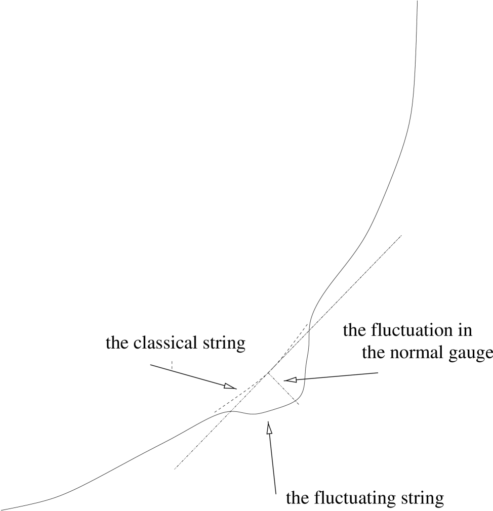
Figure 1: The fluctuations in the normal gauge

We denote the magnitude of the fluctuation along the normal direction by the dimensionless field $\xi_{n}(u_{cl},t)$. The coordinate vector in the $(x,u)$ plane is thus

$$x=x_{cl}(u_{cl})+n_{x}(u_{cl})\,\xi_{n}(u_{cl},t)\;,\;u=u_{cl}+n_{u}(u_{cl})\,\xi_{n}(u_{cl},t)$$ (21)

and both $u_{cl}$ and $x_{cl}$ change after the fluctuation to the final values $u$ and $x$.

Unlike the fixed $u$ gauge, the fluctuations result also in a change in the metric. In our gauge the off-diagonal elements are zero and the diagonal elements, to second order, are given by:

$$G_{\mu\mu}(X) = G_{\mu\mu}(u_{cl})+\partial_{u}G_{\mu\mu}(u_{cl})\cdot n_{u}(u_{cl})\,\xi_{n}(u_{cl},t)$$ (22)

$$+ \frac{1}{2}\partial_{u}^{2}G_{\mu\mu}(u_{cl})\cdot\left(n_{u}(u_{cl})\,\xi_{n}(u_{cl},t)\right)^{2}$$

(with no summation over indices). As the action is an integral of ${\cal L}$ essentially from $u=\infty$ to $u=u_{0}$ and back again to $u=\infty$, and we have the boundary conditions $\xi_{n}(\infty,t)=0$, the part of ${\cal L}$ linear in $\xi_{n}$ does not have to vanish, but rather should be a total derivative of the form $\partial_{u}(F_{(1)}\,\xi_{n}(u_{cl},t))$, in order to ensure that the classical solution is an extremum. We find this to be indeed the case. Inspection of $h_{\alpha\beta}$ readily reveals that there are in $h$ no quadratic terms of the types $\partial_{t}\xi_{n}\cdot\xi_{n}$ or $\partial_{t}\xi_{n}\cdot\partial_{u}\xi_{n}$ (and also no linear term of the type $\partial_{t}\xi_{n}$). By adding a total derivative of the type $\partial_{u}(F_{(2)}\,\xi_{n}(u_{cl},t)^{2})$ we can also get rid of the $\partial_{u}\xi_{n}\cdot\xi_{n}$ term. Finally, we get the quadratic expression

$${\cal L}_{(2)}={\cal L}_{cl}+C_{\xi\xi}(u_{cl})\xi_{n}^{2}+C_{tt}(u_{cl})(\partial_{t}\xi_{n})^{2}+C_{uu}(u_{cl})(\partial_{u}\xi_{n})^{2}$$ (23)

Thus the operator ${\cal O}_{n}$ takes the form

$${\cal O}_{n}=-\partial_{u}(C_{uu}(u_{cl})\partial_{u})-C_{tt}(u_{cl})\partial_{t}^{2}+C_{\xi\xi}(u_{cl})$$ (24)

Since the explicit expressions of the $C$’s are cumbersome for the general case we do not find it useful to write them down. In sections 6, 12 we derive them for certain special cases.

3.3 The fixed $x$ gauge

Here we impose $\sigma=x$ and fix the gauge by $\xi_{x}=0$. Expanding now the square root of $h$ to quadratic order yields yet another operator for the longitudinal fluctuations. We write it this time in the form of the action.

$$S_{(2)}={f(u_{0})\over 2}\int d\sigma d\tau\left\{\left[{{g(u)^{2}f(u_{0})^{2}}\over{f(u)^{4}}}\left(\partial_{\sigma}\xi_{u}\right)^{2}+{G_{uu}({u})\over G_{tt}({u})}\left(\partial_{\tau}\xi_{u}\right)^{2}+\mu^{2}(\sigma)\xi_{u}^{2}\right]\right.$$

$$\left.+\left[{G_{y_{i}y_{i}}({u})\over G_{xx}({u})}\left(\partial_{\sigma}\xi_{i}\right)^{2}+{{G_{y_{i}y_{i}}({u})G_{xx}({u})}\over f(u_{0})^{2}}\left(\partial_{\tau}\xi_{i}\right)^{2}\right]\right\}$$ (25)

The ”mass term” $\mu^{2}(\sigma)$ will be written explicitly for specific metrics. The fact that there is a ”mass” term present in this gauge, and in the normal coordinate gauge, and there is no such term in the fixed $u$ gauge is not surprising since such a term necessarily arises when $G_{\mu\nu}(u)$ is expanded about ${u_{cl}}$. In the gauge $\sigma=u$ there is no fluctuation in $u$ so no such term arises. The significance of this term will be discussed further when we study special cases such as AdS and pure Yang-Mills.

3.4 Comparing the different gauges

One expects that physical, gauge invariant quantities should be identical when using different gauges. This general belief is justified provided that one considers legitimate gauges. The differential operators derived in the three different gauges are manifestly not identical. It may happen that their determinant is nevertheless identical. Formally, one can pass from one gauge to another. For instance changing the integration variable from $\sigma=x$ to $\sigma=u$ together with the rescaling of $\xi_{u}$

$$\xi_{u}=\xi_{x}\cdot\partial_{x}{u}(x)$$ (26)

maps between the fixed $x$ gauge to the fixed $u$ one. However, this rescaling itself may be singular as indeed occurs at $u_{0}$.

The computation of the operator ${\cal O}_{x}$ in the fixed $u$ gauge corresponds to the assumption that the longitudinal fluctuation of the string is in the $x$ direction (”gauge fixing” the coordinates $u,t$ as $\sigma,\tau$ respectively). This assumption leads to two problems in the physical interpretation. First, near $u=u_{0}$, even a small fluctuation can lead to multiple valuedness of $x$ as a function of $u$. Second, the extremal point can itself fluctuate in the $u$ direction, and no longer correspond to $u=u_{0}$ (see figure 2). The problem is that at $u=u_{0}$ the $x$ direction is tangential to the classical curve, and that choice of the direction of the field of fluctuations becomes singular. As the metrics depend only on $u$, this choice of fluctuation involves no change in metric. It is easy to understand, therefore, why the operator ${\cal O}_{x}$ involves only derivatives of the fluctuating field.

By choosing $\sigma$ to be $x$, and the direction of fluctuations to be along $u$, the limit $u=\infty$ becomes singular in the aforementioned sense. However, this singularity exists also in the fluctuations of the bare quarks, and after the subtraction of the quark masses from (8) it might cancel.

The safest choice, however, seems to be taking the fluctuations to be anywhere normal to the classical curve, as previously explained.

Figure 2: A problematic fluctuation in the fixed $u$ gauge

4 Bosonic string in flat space-time

We can now easily derive the free energy of a bosonic string in flat space-time (Lüscher term). The metric is given by $G_{tt}=-1\;;\;G_{xx}=G_{y_{i}y_{i}}=1$, where $i=1,\ldots,D-2$. Note that $u$ is now one of the $y_{i}$ coordinates. The classical solution in this case is just a straight line along the $x$ direction from $-L/2$ to $L/2$. Obviously, for this case the three different gauges are identical. We use (3.1) and regard only the transverse fluctuations operator ($\hat{\cal O}_{y_{i}}$). This operator is the ordinary Minkowski Laplacian. Considering now Euclidean space time and demanding the eigenfunctions to vanish on the boundary, the eigenvalues of the Laplacian are (minus)

$$E_{n,m}=({{n\pi\over L}})^{2}+({{m\pi}\over T})^{2}$$ (27)

and the free energy is given by

$$-\frac{2}{D-2}F_{B} = \log\det\Delta=\log\prod_{n,m}E_{n,m}=\sum_{n,m}\>\log(({n\pi\over L})^{2}+({m\pi\over T})^{2})$$

$$\sim \sum_{n}\>{T\over\pi}\int_{0}^{\infty}d\omega\log(1+({n\pi\over\omega L})^{2})+o(L)=\sum_{n}{T\over\pi}\cdot\pi\cdot{n\pi\over L}+o(L)$$

$$= T{\pi\over L}\sum_{n}n+o(L)$$ (29)

where we assumed that $T$ is large.

Regulating this equation using the Riemann zeta function and discarding (infinite) terms that do not depend on L, we find

$$F_{B}=(D-2){\pi\over 24}{T\over L}$$ (30)

This expression also gives a quantum correction to the linear quark anti-quark potential in a bosonic QCD-string model in D-dimensional flat space. Using the Wilson loop to calculate this potential we have

$$\Delta V(L)=-{1\over T}F_{B}=-(D-2){\pi\over 24}\cdot{1\over L}$$ (31)

which is called the Lüscher term.

5 A General scaling result

The argument of the previous section can be generalized to operators which do not necessarily correspond to the flat case and will lead to a general scaling result that will prove useful in our work.

Let us define the operators

$${\cal O}[A,B]=A^{2}F_{t}(v)\partial_{t}^{2}+B^{2}{\cal O}_{v}$$ (32)

with $t$ the time, $v$ a coordinate whose range is independent of $L$. ${\cal O}_{v}$ is a general operator of $v$ alone, independent of $L$, and $A,B$ are constants which may depend on $L$. Then, $V[A,B]$, defined as the correction to the potential arising from ${\cal O}[A,B]$, is proportional to $B/A$. In particular, the potential is independent of any overall factor multiplying the operator ${\cal O}$.

The idea of the proof is that by redefining $t$ we can scale the operator ${\cal O}[A,B]$ to ${\cal O}[1,1]$, and the factors by which the eigenvalues get multiplied in this operation become irrelevant in the large $T$ limit. We proceed to the proof itself.

Separation of variables shows that the eigenfunctions of ${\cal O}[A,B]$ are $\phi(v,t)=e^{i\omega t}\phi(v)$. We define the eigenvalues $\tilde{E}_{n}(\omega^{\prime})$ by

$$\left[-F_{t}(v)\,\omega^{\prime 2}+{\cal O}_{v}\right]\tilde{\phi}(v)=\tilde{E}_{n}(\omega^{\prime})\,\tilde{\phi}(v)$$ (33)

and $E_{n}(\omega^{\prime})$ by

$$\left[-A^{2}F_{t}(v)\,\omega^{\prime 2}+B^{2}{\cal O}_{v}\right]\phi(v)=E_{n}(\omega^{\prime})\,\phi(v)$$ (34)

or

$$\left[-F_{t}(v)(A\omega^{\prime}/B)^{2}+{\cal O}_{v})\right]\phi(v)=B^{-2}E_{n}(\omega^{\prime})\,\phi(v)$$ (35)

so that

$$E_{n}(\omega^{\prime})=B^{2}\tilde{E}_{n}(A\omega^{\prime}/B)$$ (36)

The boundary conditions for the time coordinate lead to $\omega=\frac{\pi m}{T}$ for integer $m$. Hence we have for $V[A,B]$, (when $o(T)$ designates a term which does not depend on $T$, or grows sublinearly with it),

$$-T\cdot V[A,B]+o(T) = \frac{1}{2}\log\det{\cal O}[A,B]$$ (37)

$$= \frac{1}{2}\sum_{n}\sum_{m}\log E_{n}(\frac{\pi m}{T})$$

$$= \frac{1}{2}\sum_{n}\sum_{m}\left(\log\tilde{E}_{n}(\frac{A}{B}\cdot\frac{\pi m}{T})+2\log B\right)$$

$$= \frac{1}{2}\sum_{n}\sum_{m}\left(\log\tilde{E}_{n}(\frac{\pi m}{BT/A})\;+\;o(T)\right)$$

$$= -\frac{BT}{A}\cdot V[1,1]+o(T)$$

and so indeed $V[A,B]=(B/A)\cdot V[1,1]$.

We can make a simple consistency check of our result. Let us look at the flat Laplacian $\Delta=\partial_{t}^{2}+\partial_{x}^{2}$. The range of $v=x/L$ is $0\leq v\leq 1$ independent of $L$, and $\Delta=\partial_{t}^{2}+L^{-2}\partial_{v}^{2}$, so by the above result we get $V(L)\propto L^{-1}$ as we have indeed seen in section 4.

6 Bosonic string in the $AdS_{5}\times S^{5}$ background

In $AdS_{5}\times S^{5}$ background the metric can be written in the following form

$$-G_{tt}=G_{xx}=G_{yy}={u^{2}\over R^{2}};~{}~{}G_{uu}={R^{2}\over u^{2}};~{}~{}G_{\zeta\zeta}=R^{2}$$ (38)

where $y$ is a transverse coordinate of the $AdS_{5}$, while $\zeta$ is a transverse coordinate in $S^{5}$. We therefore get

$$f(u) = {u^{2}\over R^{2}}$$ (39)

$$g(u) = 1$$ (40)

Note that as we deal with small fluctuations and big $R$, the angular coordinates $\zeta$ of $S^{5}$ can be treated as if they were not compactified.

Unlike the flat case, for the $AdS_{5}\times S^{5}$ metric the different gauge fixings yield different operators.

In the fixed $u$ gauge one finds using (3.1) the following quadratic operators

$$\hat{\cal O}_{x}={1\over 2}{u_{0}^{2}\over R^{2}}\left[\partial_{x}((1-{u_{0}^{4}\over u^{4}})\partial_{x})-({u^{4}\over u_{0}^{4}}-1)\partial_{t}^{2}\right]$$ (41)

and

$$\hat{\cal O}_{y} = {1\over 2}{u_{0}^{2}\over R^{2}}\left[\partial_{x}^{2}-{u^{4}\over u_{0}^{4}}\partial_{t}^{2}\right]$$

$$\hat{\cal O}_{\zeta} = {1\over 2}{u_{0}^{2}\over R^{2}}\left[\partial_{x}(\frac{R^{4}}{u^{2}}\partial_{x})-\frac{R^{4}u^{2}}{u_{0}^{4}}\partial_{t}^{2}\right]$$ (42)

In the normal fluctuations gauge, the fluctuations along the directions $y,\zeta$ which are perpendicular to the $(x,u)$ plane are the same as (42). However, for ${\cal O}_{n}$ we have

$${\cal O}^{\prime}_{n}=\frac{2u^{8}-5u^{4}u_{0}^{4}+3u_{0}^{8}}{2u^{6}\sqrt{u^{4}-u_{0}^{4}}}-\frac{R^{4}}{2\sqrt{u^{4}-u_{0}^{4}}}\;\partial_{t}^{2}-\partial_{u}\left(\frac{\sqrt{u^{4}-u_{0}^{4}}}{2}\,\partial_{u}\right)$$ (43)

In the dimensionless variable $v=u/u_{0}$, it is easy to see that this operator is of the form (32), with $A^{2}=R^{4}u_{0}^{-2},\;B^{2}=1$. We conclude, according to the result of section 5, that the correction to the potential is proportional to $R^{-2}u_{0}$, that is [8], inversely proportional to $L$. Moreover, there is no further dependence on $R$ when we eliminate the variable $u_{0}$ in favour of $L$. The classical and quadratic quantum quark anti–quark potential add up to $V\sim-\sqrt{\lambda}/L+c^{\prime}/L$ with $\lambda\equiv g_{YM}^{2}N\sim R^{4}$ the ’t Hooft coupling constant, and $c^{\prime}$ a universal constant, independent of $\lambda$. We see that the quantum expansion in $\hbar$ is equivalent, for large $\lambda$, to an expansion in $R^{-2}$ or equivalently in $\lambda^{-1/2}$. The quantum expansion does not spoil, of course, the conformal nature of the field theory. The other operators for the normal gauge can be seen, by similar reasoning, to give rise also to a potential correction of the same characteristics.

Note also that if we approximate the classical curve to be flat over most of its range and thus approximate $u=u_{0}$ throughout, the mass term drops out and the operator simplifies to the flat Laplacian,

$$\hat{\cal O}^{\prime}_{x}\longrightarrow-\frac{1}{2}\,\partial_{t}^{2}-\frac{1}{2}\,\partial_{x}^{2}$$ (44)

and for the longitudinal direction we get exactly the same Lüscher term as in the flat case. The same happens also to the transverse directions. (Note that ${\cal O}_{n}^{\prime}$ cannot be approximated in this way since $u$ is constant and it is thus not integrated over ). The shape of the string, however, does not change with $L$ but only scales. It is thus not a good approximation, in our case, to assume that the string is flat. In section 11 we will give quite a stringent criterion for flatness, and prove that strings in metrics corresponding to confining field theories are indeed flat.

When we revert to a differential operator involving the coordinate $x$ instead of $u$, (with the integration of the Lagrangian in the $t,x$ coordinates), the operator (43) is translated to

$$\hat{\cal O}^{\prime}_{n}=\frac{2u^{8}-5u^{4}u_{0}^{4}+3u_{0}^{8}}{2R^{2}u^{4}u_{0}^{2}}-\frac{R^{2}u^{2}}{2u_{0}^{2}}\;\partial_{t}^{2}-\partial_{x}\left(\frac{R^{2}u_{0}^{2}}{2u^{2}}\,\partial_{x}\right)$$ (45)

In the fixed $x$ gauge we have again the same transverse operators, while the longitudinal operator becomes

$$\hat{\cal O}^{\prime}_{x}=\frac{5u_{0}^{6}-2u^{4}u_{0}^{2}}{u^{6}R^{2}}+\frac{u_{0}^{2}R^{2}}{2u^{4}}\;\partial_{t}^{2}+\partial_{x}\left(\frac{u_{0}^{6}R^{2}}{2u^{8}}\,\partial_{x}\right)$$ (46)

Note that we can use the same scaling arguments as for the normal gauge to show that the correction is inversely proportional to $L$. Another remark is in order. The “mass term” is more properly looked at as a shift in the levels of the massless modes rather than as a real mass term, since it behaves like $u_{0}^{2}/R^{4}$ which is proportional to $1/L^{2}$. Thus the mass gap in this case will be of the same order as the energy of a massless mode in a box of length $L$.

7 The bosonic string in the $AdS_{5}\times S^{5}$ background – Polyakov’s action

The analysis of the quadratic quantum fluctuations can be performed, as was discussed at the end of section 2, also in the framework of Polyakov’s action. Here we present a rederivation of the bosonic determinant of the $AdS_{5}\times S^{5}$ Wilson loop using the Polyakov action. Recall that the action (2) is given by

$$S={1\over 2}\int d\sigma d\tau\sqrt{h}h^{\alpha\beta}\partial_{\alpha}X^{\mu}\partial_{\beta}X^{\nu}G_{\mu\nu}(X)$$ (47)

with the metric given in (38). This action is minimized by the classical configuration

$$u(\sigma,\tau)=u_{cl}(\sigma);~{}~{}t(\sigma,\tau)=\tau;~{}~{}x(\tau,\sigma)=\sigma;~{}~{}y^{i}(\sigma,\tau)=0;~{}~{}\zeta_{I}(\sigma,\tau)=0$$ (48)

The function $u_{cl}(\sigma)$ satisfies the equation [8]

$$\int_{1}^{u_{cl}/u_{0}}{{dy}\over{y^{2}\sqrt{y^{4}-1}}}={{\sigma u_{0}}\over R^{2}}$$ (49)

where $u_{0}=u(\sigma=0)$, the minimal value of $u_{cl}$, is determined by the boundary conditions at $\sigma=\pm L/2$ where $u\rightarrow\infty$, to be

$$u_{0}=\frac{2\sqrt{2}{\pi}^{3/2}R^{2}}{\Gamma(\frac{1}{4})^{2}}\cdot L^{-1}$$ (50)

The classical value of the worldsheet metric is determined by the equations of motion derived by variation of the action with respect to $h_{\alpha\beta}$,

$$h_{\alpha\beta}=\partial_{\alpha}X^{\mu}\partial_{\beta}X^{\nu}G_{\mu\nu}(X)$$ (51)

which take the following form

$$({h_{\sigma\sigma}})_{cl}={u_{cl}^{6}\over{u_{0}^{4}R^{2}}}\qquad({h_{\tau\tau}})_{cl}={u_{cl}^{2}\over R^{2}}$$ (52)

The quantum fluctuations of the string coordinates are introduced as in (12), and those of the world sheet metric are as follows

$$h_{\sigma\sigma}=(h_{\sigma\sigma})_{cl}(1+\gamma_{\sigma});\qquad h_{\tau\tau}=(h_{\tau\tau})_{cl}(1+\gamma_{\tau});\qquad h_{\sigma\tau}=\gamma\sqrt{(h_{\sigma\sigma})_{cl}(h_{\tau\tau})_{cl}}$$ (53)

where $\gamma,\gamma_{\sigma},\gamma_{\tau}$ parameterize the metric fluctuations.

We now use the reparameterization invariance of the action to choose the “gauge” in which

$$\xi^{u}(\sigma,\tau)=\xi^{t}(\sigma,\tau)=0$$ (54)

so that

$$u=u_{cl}(\sigma);~{}~{}x^{t}=\tau;~{}~{}x^{1}=\sigma+\xi^{1};~{}~{}x^{2}=\xi^{2};~{}~{}x^{3}=\xi^{3}$$ (55)

Note that we do not consider here the fluctuations in the $\zeta$ directions.

Next we expand the action (47) to quadratic order in the $\gamma$’s and the $\xi$’s. The first order correction of the classical action $S_{(1)}$ is expected to vanish and indeed

$$S_{(1)}={u_{0}^{2}\over R^{2}}\int d\sigma d\tau\partial_{\sigma}\xi^{1}$$ (56)

vanishes by the boundary conditions on $\xi^{1}$. The quadratic term is given by:

$$S_{(2)}={1\over 2}\int d\sigma d\tau\left[{u_{cl}^{4}\over{R^{2}u_{0}^{2}}}\left\{\gamma^{2}+{1\over 4}\left(\gamma_{\tau}-\gamma_{\sigma}\right)^{2}+\left(\partial_{\tau}\xi^{i}\right)^{2}\right\}\right.$$

$$\left.+{u_{0}^{2}\over R^{2}}\left\{\left(\partial_{\sigma}\xi^{i}\right)^{2}+\partial_{\sigma}\xi^{1}\left(\gamma_{\tau}-\gamma_{\sigma}\right)\right\}-{{2u_{cl}^{2}}\over R^{2}}\gamma\partial_{\tau}\xi^{1}\right]$$ (57)

Our next step is to perform the Gaussian integrals over the $\gamma$’s. Recall that our goal is to compute

$${{\cal{Z}}_{(2)}}=\int{\cal{D}}h_{\alpha\beta}\prod_{i=1}^{3}{\cal{D}}\xi^{i}\exp\left\{-S_{(2)}\right\}$$ (58)

where we integrate over the fluctuations of $h_{\alpha\beta}$. This can be translated to integrations of the various $\gamma$’s. The result of the integral is:

$${{\cal{Z}}_{(2)}}=\prod_{i=1}^{3}{\cal{D}}\xi^{i}\exp\left\{-S_{\rm eff}\right\}$$ (59)

with

$$S_{\rm eff}={1\over 2}\int d\sigma d\tau\left[{u_{0}^{2}\over R^{2}}\left\{\left({u_{cl}^{4}\over u_{0}^{4}}-1\right)\left(\partial_{\tau}\xi^{1}\right)^{2}+\left(1-{u_{0}^{4}\over u_{cl}^{4}}\right)\left(\partial_{\sigma}\xi^{1}\right)^{2}\right\}\right.$$

$$\left.+\left\{{u_{cl}^{4}\over{R^{2}u_{0}^{2}}}\left(\partial_{\tau}\xi^{\perp}\right)^{2}+{u_{0}^{2}\over R^{2}}\left(\partial_{\sigma}\xi^{\perp}\right)^{2}\right\}\right]$$ (60)

where the notation $\xi^{\perp}$ refers to $\xi^{2}$ and $\xi^{3}$. It is thus clear that in the fixed $u$ gauge the bosonic operators derived from Polyakov’s action are identical to those found from the NG action (42).

8 Introducing fermionic fluctuations

So far we have considered only quantum fluctuations of the bosonic degrees of freedom. Recall, however, that gauge/gravity duality was originally [7] proposed in the context of superstring theories which include worldsheet fermions. This, together with the hope that supersymmetry will lead to the cancellation of divergences, raises the question of the contribution of fermionic fluctuations to the free energy. It might seem an easy task to truncate the NSR action and collect terms quadratic in the fermionic fluctuations. This is indeed the case for a flat background with vanishing Ramond–Ramond form. However there is so far no satisfactory formulation of the world-sheet supersymmetric NSR action for a background with non-vanishing RR forms. Recall that in the $AdS_{5}\times S^{5}$ model, the self dual 5-form plays an essential role. Hence we use here the manifestly space-time supersymmetric GS approach. For the $AdS_{5}\times S^{5}$ background this action has been constructed in [24] as a supersymmetric sigma model with the coset supermanifold $SO(2,2|4)/(SO(1,4)\times SO(5))$ as its target space. The GS action is invariant under local $\kappa$-symmetry. By gauge fixing this symmetry one reduces the number of fermionic degrees of freedom by a factor of two so that it matches the number of bosonic degrees of freedom. In [27] a 2d scalar-scalar duality transformation was invoked to transform the gauge fixed action into an action which is quadratic in the fermions.

In this section we first consider the fermionic contribution of the supersymmetric theory in flat space-time. We then use the gauge fixed action [27] to deduce the contribution of the fermionic quantum correction in the $AdS_{5}\times S^{5}$ background.

8.1 Fermions in flat space-time

For flat Minkowski space-time we choose the super-Poincaré group as our target space. When we explicitly consider a flat classical string, the fermionic part of the simplified gauge fixed GS-action in the flat space-time is simply

$$S_{F}^{flat}=2i\int d\sigma d\tau\bar{\theta}\Gamma^{i}\partial_{i}\theta$$ (61)

where $\theta$ is a Weyl-Majorana spinor and $\Gamma^{i}$ are the SO(1,9) gamma matrices. The fermionic operator is, hence

$$\hat{\cal O}_{F}=D_{F}=\Gamma^{i}\partial_{i}$$ (62)

and squaring it we get $\Delta=\partial_{x}^{2}-\partial_{t}^{2}$ . The total free energy of the supersymmetric case is therefore (using the fact that for D=10, we have 8 transverse coordinates and 8 components of a Weyl-Majorana spinor),

$$F=8\times\left(-{1\over 2}\log\det\Delta+\log\det D_{F}\right)=0$$ (63)

and there is no Lüshcer term.

8.2 Fermions in $AdS_{5}\times S^{5}$

The target space for the GS action in the $AdS_{5}\times S^{5}$ background is the coset superspace $SU(2,2|4)/(SO(1,4)\times SO(5))$ [24]. The action is found to be in the form of the usual supersymmetric string action (but with the induced non–flat metric), with a change of the derivative acting on the spinor variables $\theta^{1},\theta^{2}$. If $e_{i}^{a}$ is the induced worldsheet vielbien, and $\omega_{i}^{ab}$ the induced worldsheet spin connection, then

$$\partial_{i}\theta^{I}\rightarrow D_{i}\theta^{I}\equiv{\cal D}_{i}\theta^{I}-{i\over 2}\epsilon^{IJ}e_{i}^{a}\gamma^{a}\theta^{J}$$ (64)

with ${\cal D}_{i}=\partial_{i}+{1\over 4}\omega_{i}^{ab}\gamma_{ab}$ the usual induced worldsheet covariant derivative. The interpretation is that the metric influences the action through ${\cal D}_{i}$ while the Ramond–Ramond flux is responsible for the second term in (64). Using the gauge fixing suggested in [25, 26, 27], the fermionic part of the action for the classical solution can be computed and it leads to the operator

$$\hat{\cal O}_{F}={u_{0}^{2}\over R^{2}}\Gamma^{1}\partial_{x}+\left({u_{cl}^{4}\over{u_{0}^{2}R^{2}}}\Gamma^{0}+{u_{cl}^{2}\over R^{4}}\cdot{\sqrt{u_{cl}^{4}-u_{0}^{4}}\over u_{0}^{2}}\Gamma^{2}\right)\partial_{t}$$ (65)

where we use gamma matrices of SO(1,4) which is the $AdS_{5}$ tangent space. Squaring this operator, we find

$$\left({R^{2}\over u_{0}^{2}}\hat{\cal O}_{F}\right)^{2}=\partial_{x}^{2}-{u_{cl}^{4}\over u_{0}^{4}}\partial_{t}^{2}={R^{2}\over u_{0}^{2}}\hat{\cal O}_{y}$$ (66)

We find therefore, that the transverse fluctuations partially cancel the fermionic fluctuations and we are left with six fermionic degrees of freedom and the longitudinal and angular bosonic fluctuations.

9 Bare quark in $AdS_{5}\times S^{5}$

In this section we investigate the single ”bare” quark, which is a flat string in $AdS_{5}\times S^{5}$ space stretching along the $AdS$ radial coordinate . In this case the string is a BPS state and we expect neither its charge nor its mass to be modified by quantum fluctuations. This problem is related to issues associated with certain BPS soliton solutions [31].

The $AdS_{5}\times S^{5}$ metric is

$$ds^{2}=G_{MN}dx^{M}dx^{N}=\left(\frac{R^{2}}{u^{2}}\right)du^{2}+\left(\frac{u^{2}}{R^{2}}\right)dx_{\mu}dx^{\mu}+R^{2}d\Omega_{5}^{2}$$ (67)

where we take $\{x_{0},x_{1},x_{2},x_{3}\}$ with Minkowskian signature.

The classical solution of the bare quark is $\sigma=u,\tau=t,x_{i}=0$ and the $S^{5}$ angles $\zeta_{I}$=0. It is obvious that there is a separation of the quadratic action, and the fluctuations of the fields can be taken one at a time. We shall take the static gauge of the action, so that the fluctuating fields are the three $x_{i}$ and the five $\zeta_{I}$.

For the five angular fields, since we are working in the large $R$ regime, the curvature of $S^{5}$ is not felt, and we can approximate $S^{5}$ locally by the flat space ${\bf R}^{5}$. We take one field $\phi(\sigma,\tau)$ along one angle $\zeta$, i.e, study the worldsheet with $(u,t,\zeta)=(\sigma,\tau,\phi(\sigma,\tau))$. We have

$$h_{\alpha\beta}=G_{MN}\partial_{\alpha}x^{M}\partial_{\beta}x^{N}=\left(\begin{array}[]{cc}-(u/R)^{2}+R^{2}\dot{\phi}^{2}&R^{2}\phi^{\prime}\dot{\phi}\\ R^{2}\phi^{\prime}\dot{\phi}&(R/u)^{2}+R^{2}\phi^{\prime 2}\end{array}\right)$$ (68)

so that

$$h=\det h_{\alpha\beta}=-1+(R^{4}/u^{2})\dot{\phi}^{2}-u^{2}\phi^{\prime 2}$$ (69)

The Nambu–Goto action (2) is therefore $S\propto\sqrt{-h}=1+S_{(2)}+O(\phi^{4})$ with the quadratic action

$$S_{(2)}\propto(R/u)^{2}\dot{\phi}^{2}-(u/R)^{2}\phi^{\prime 2}=\phi\left[-(R/u)^{2}\partial_{t}^{2}+(u/R)^{2}\partial_{u}^{2}-1/R^{2}\right]\phi$$ (70)

where we have used integration by parts and the Dirichlet boundary conditions. We therefore see that for the five angular bosonic fluctuations, the quadratic operator is ${\cal O}=-(R/u)^{2}\partial_{t}^{2}+(u/R)^{2}\partial_{u}^{2}-1/R^{2}$.

For the three spatial coordinates, we want to keep the fluctuating field dimensionless, so we take $(u,t,x)=(\sigma,\tau,\phi(\sigma,\tau)/u)$. A similar calculation yields in this case the operator ${\cal O}=-(R/u)^{2}\partial_{t}^{2}+(u/R)^{2}\partial_{u}^{2}-3/R^{2}$.

Regarding the fermionic fluctuations around the classical bare quark configuration, one can see that the $\kappa$-symmetry fixing suggested at [25, 27] is not applicable, and produces a degenerate operator. We should therefore consider only the quadratic part of the action and try another way to fix the gauge. The quadratic part of the GS action is, in this case,

$${\cal L}_{F}^{(2)}= \bar{\theta^{0}}\left[-i{R\over u}\gamma^{0}{\cal D}_{0}+i{u\over R}\gamma^{4}{\cal D}_{1}-i{u\over R}\gamma^{0}{\cal D}_{1}+i{R\over u}\gamma^{4}{\cal D}_{0}\right]\theta^{0}$$

$$+ \bar{\theta^{1}}\left[-i{R\over u}\gamma^{0}{\cal D}_{0}+i{u\over R}\gamma^{4}{\cal D}_{1}+i{u\over R}\gamma^{0}{\cal D}_{1}-i{R\over u}\gamma^{4}{\cal D}_{0}\right]\theta^{1}$$

$$+ \bar{\theta^{0}}\left[1-\gamma^{0}\gamma^{4}\right]\theta^{1}+\bar{\theta^{1}}\left[-1-\gamma^{0}\gamma^{4}\right]\theta^{0}$$

Fixing the $\kappa$-symmetry by setting $\theta^{0}=\theta^{1}$ and writing the covariant derivative explicitly, ${\cal D}_{0}=\partial_{0}+(u/2)\gamma^{0}\gamma^{4}\;,\;{\cal D}_{1}=\partial_{1}$, we have

$${\cal O}_{F}=-{R\over u}\gamma^{0}\partial_{t}+{u\over R}\gamma^{4}\partial_{u}+{1\over{2R}}\gamma^{4}+{i\over R}\gamma^{0}\gamma^{4}$$ (72)

Squaring this operator, integrating by parts and ignoring total derivatives, we find the operator

$${\cal O}_{F}^{2}=-(R/u)^{2}\partial_{t}^{2}+(u/R)^{2}\partial_{u}^{2}-{{7/4}\over{R^{2}}}$$ (73)

One should note, however, that taking another gauge fixing, which is a-priori as good as ours (e.g. $\theta^{1}=-i\gamma^{3}\theta^{0}$) leads to a different result. We prefer our gauge fixing as it leads to the expected cancelation of the divergences.

All the quadratic operators of the dynamical degrees of freedom are seen to be of the form ${\cal O}_{j}=-(R/u)^{2}\partial_{t}^{2}+(u/R)^{2}\partial_{u}^{2}-c_{j}/R^{2}$. There are eight bosonic ones, corresponding to the eight coordinates left after fixing the worldsheet reparameterizations, and eight fermionic ones. The fermionic operators were squared, and are taken with a negative sign, as the fields are complex Grassmannian. Therefore, The quadratic quantum contribution to the mass is

$$\Delta m=-\frac{1}{2T}\left(\sum_{\mbox{bosons }}\log\det{\cal O}_{j}\;\;-\sum_{\mbox{fermions}}\log\det{\cal O}_{j}\right)$$ (74)

We were unable to find explicitly the eigenvalues of those operators and multiply them using some regularization scheme. However, it is well known that the logarithm of the determinant of such second order operators has in general quadratic, linear and logarithmic divergences in the cutoff scale $\Lambda$. Moreover, the corresponding coefficients are known (see, for example, [5]). The sheer fact that the number of fermionic and bosonic operators is the same, and that they differ only in the ”mass term” $c_{j}/R^{2}$ is sufficient to ensure that the quadratic and linear divergences cancel out in (74). The logarithmic divergence also cancels out provided that

$$\sum_{\mbox{bosons }}c_{j}\;\;-\sum_{\mbox{fermions}}c_{j}\;\;=\;\;0$$ (75)

Indeed, we have $3\cdot 3+5\cdot 1-8\cdot 7/4=0$. We therefore see that there is no infinite part, needing renormalization, to the aforementioned contribution to the bare quark mass. We were unable to show, however, that the finite part also vanishes, as expected from supersymmetry.

10 Fluctuations of the $D_{p}$ backgrounds

In this section we show that the quadratic contribution of the quantum fluctuations to the potential is proportional to $1/L$ in the general Dp background ($p\leq 4$). In the D3 case, where the result is dictated by conformality, this was shown in section 6.

For metrics relevant to $Dp$-branes, $-G_{tt}=G_{xx}=G_{yy}$ and

$$f(u) = au^{k}$$ (76)

$$g(u) = bu^{j}$$ (77)

with arbitrary $a,b\neq 0\;,\;k,j$ (for those specific metrics, $a\sim R^{-(7-p)/2}$). The power-like behaviour of $f,g$ is essential in order to get the desired result.

The operator for transverse fluctuations is given by (3.1). Inserting $f,g$ to that equation and changing the variable $u$ to $v=u/u_{0}$ (which has the range $1\leq v<\infty$ regardless of $L$), we get

$${\cal O}_{y}={1\over 2}\left[bu_{0}^{j}\cdot{{v^{j}}\over\sqrt{1-v^{-2k}}}\partial_{t}^{2}+\frac{a^{2}}{b}u_{0}^{2k-j-2}\cdot\partial_{v}\left(v^{2k-j}\sqrt{1-v^{-2k}}\partial_{v}\right)\right]$$ (78)

Which is of the form (32) with $A^{2}=bu_{0}^{j}\;,\;B^{2}=\frac{a^{2}}{b}u_{0}^{2k-j-2}$. Therefore, by the result of section 5, the potential is proportional to $B/A=\frac{a}{b}u_{0}^{k-j-1}$. As it is known [17] that $L\propto\frac{b}{a}u_{0}^{j+1-k}$, we finally get that $V\propto L^{-1}$, that is, the correction to the potential resulting from transversal bosonic fluctuations (and from all fermionic ones) is inversely proportional to $L$. Unfortunately, we do not know the constant of proportionality, and not even its sign. This constant of proportionality, however, cannot depend on $R$ since the constants $a,b$ cancel out. Indeed, for $p\neq 3$, the ’t Hooft coupling constant $\lambda\sim R^{7-p}$ is dimensionful, and therefore can not enter the aforementioned constant of proportionality. The classical and quantum quadratic potentials add up to $V\sim-\lambda^{1/(5-p)}/L^{2/(5-p)}+c^{\prime}/L$ and the quantum expansion is in $\lambda^{-1/(5-p)}$.

One can easily see that the scaling for the longitudinal bosonic operator ${\cal O}_{x}$ in the fixed $u$ gauge is essentially identical, as it can be casted to the form (32) with the same $A,B$ as in the transverse case. Therefore we conclude that the correction arising from this gauge fixing also obeys $V\propto L^{-1}$. The picture in the normal gauge, which we argued is safer, is more involved. We have computed it explicitly and shown the $L^{-1}$ behaviour only in the $p=3$ case.

11 Flatness of the string in the confining case

The string in the confining “pure Yang-Mills” case was shown [19] to be very flat for large $L$. This result will be needed for the next section. In this section we shall generalize this result in a precise manner for all metrics giving confinement. We shall pick a constant value $w$ (independent of $L$) and inquire at what distance $d$ from the ends of the string (at $x=\pm L/2$) the string reaches $u=w$. We shall find that we cannot show that $d$ is independent of $L$ but rather we find that it can grow with $L$. This growth is however mild and the ratio $d/L$ tends to zero as $L$ grows (see figure 3).

The analysis requires the Taylor expansion of $f(u)$ and $g(u)$ (we use the conventions of [17]),

$$f(u) = f(0)+a_{k}u^{k}+O(u^{k+1})$$ (79)

$$g(u) = b_{j}u^{j}+O(u^{j+1})$$ (80)

with $f(0)\neq 0$ due to confinement. We pick $w$ to be sufficiently small so that all our subsequent approximations are valid.

For small $u$, substitution of (79),(80) in (6) gives

$$u^{\prime}\equiv\partial_{x}u\approx\frac{\sqrt{2f(0)a_{k}(u^{k}-u_{0}^{k})}}{b_{j}u^{j}}$$ (81)

or, with $v\equiv u/u_{0}$,

$$v^{\prime}\approx\frac{\sqrt{2f(0)a_{k}}}{b_{j}}\;u_{0}^{k/2-j-1}\;\frac{\sqrt{v^{k}-1}}{v^{j}}\equiv c\;u_{0}^{k/2-j-1}\;\frac{\sqrt{v^{k}-1}}{v^{j}}$$ (82)

The critical case $k=2(j+1)$ is the generic one ($k=2,\;j=0$) and also corresponds to the “pure Yang–Mills” case ($k=1,\;j=-1/2$, where the horizon $u=u_{T}$ should be substituted for $u=0$). In this case

$$v^{\prime}\approx c\frac{\sqrt{v^{k}-1}}{v^{j}}\leq cv^{k/2-j}=cv$$ (83)

so that $(\log v)^{\prime}=v^{\prime}/v\leq c$, or $\log v\leq\log v_{0}+cx$. Therefore, $v\leq v_{0}e^{cx}$, or finally $u\leq u_{0}e^{cx}$.

If we demand $u_{0}e^{cx}\leq w$, we get

$$x\leq\frac{\log(w/u_{0})}{c}\equiv\eta-{1\over c}\log u_{0}$$ (84)

On the other hand, it is known [17] that in the critical case

$$-{1\over c}\log u_{0}={1\over 2}L+O(\log L)$$ (85)

so if $x\leq{1\over 2}L-O(\log L)$ it is guaranteed that $u\leq w$. In other words, $d\leq O(\log L)$.

In the non critical case $k>2(j+1)$, the minimum of $f(u)$ is more flat, and we expect the results to be somewhat weaker. Using arguments similar to those in the previous case (but this time not approximating $v^{k}-1\approx v^{k}$), and using results from [17], one can show that in this case $d\leq O(L^{\frac{k/2-j-1}{k/2-j}})$. $d$ can grow with $L$, but the ratio $d/L\leq O(L^{-\frac{1}{k/2-j}})$ tends indeed to zero as $L$ grows.

Figure 3: (a) The classical solution is rescaled as $L\rightarrow\infty$ in the $AdS_{5}\times S^{5}$ background while (b) It becomes flatter in the confining scenario

12 Bosonic fluctuations in the ”Pure Yang-Mills” setup

When one of the spatial coordinates of the $AdS_{5}\times S^{5}$ metric is compactified on a circle of radius $\propto u_{T}^{-1}$, with the proper boundary condition [13], the modes in the compact dimension become Kaluza-Klein modes with masses of the order of $u_{T}$, and the fermions and scalars of the conformal four-dimensional theory also acquire masses of the same order and decouple in the low energy regime of the theory. Therefore, the ${\cal N}=4$ conformal theory in four dimensions is deformed to a theory similar to non supersymmetric Yang-Mills in three dimensions.

In the brane language, the metric corresponds to non extremal $D_{3}$ branes in the near horizon limit, and $u_{T}$ is related to the energy density on the $D_{3}$ brane.

Let us call the compact direction $z$. With the conventions introduced earlier, working Euclideanly, and still neglecting factors of $2\pi$, the metric is

$$+G_{tt}=G_{xx}=G_{yy} = u^{2}/R^{2}$$ (86)

$$G_{zz} = (1-(\frac{u_{T}}{u})^{4})\cdot u^{2}/R^{2}$$ (87)

$$G_{uu} = \left((1-(\frac{u_{T}}{u})^{4})\cdot u^{2}/R^{2}\right)^{-1}$$ (88)

and so

$$f(u) = u^{2}/R^{2}$$ (89)

$$g(u) = (1-(\frac{u_{T}}{u})^{4})^{-1/2}$$ (90)

The exact classical solution for the Wilson loop in this setup is given for this case by [18, 17]

$$E=\frac{u_{T}^{2}}{2\pi R^{2}}\cdot L-2\kappa+O(e^{-\alpha L})$$ (91)

with $\kappa$ some constant and $\alpha=2u_{T}/R^{2}$.

In order to compute the quantum correction to the energy, we should compute the appropriate operators. From (3.1) we still have that

$$\hat{\cal O}_{y} = \frac{u_{0}^{2}}{2R^{2}}\left[\partial_{x}^{2}+\frac{u^{4}}{u_{0}^{4}}\partial_{t}^{2}\right]$$ (92)

$$\hat{\cal O}_{\zeta} = \frac{u_{0}^{2}}{2R^{2}}\left[\partial_{x}(\frac{R^{4}}{u^{2}}\partial_{x})+\frac{R^{4}u^{2}}{u_{0}^{4}}\partial_{t}^{2}\right]$$ (93)

but now

$$\hat{\cal O}_{z}=\frac{u_{0}^{2}}{2R^{2}}\left[\partial_{x}\left((1-(\frac{u_{T}}{u})^{4})\partial_{x}\right)+\frac{u^{4}}{u_{0}^{4}}(1-(\frac{u_{T}}{u})^{4})\partial_{t}^{2}\right]$$ (94)

A calculation for the longitudinal part using normal fluctuations, similar to that performed for the conformal case in section 6, can be carried out, and the result turns out to be similar to the longitudinal result in that case, only with a different ”mass term”.

In the large $L$ limit, as we have seen in section 11, the string is, for most of its length, very flat, and has $u\approx u_{0}$. Following [19], we assume that we can trust this analysis even after substituting $u\equiv u_{0}$ in the operators. In that limit we find

$$\hat{\cal O}_{y} \longrightarrow \frac{u_{0}^{2}}{2R^{2}}\left[\partial_{x}^{2}+\partial_{t}^{2}\right]$$ (95)

$$\hat{\cal O}_{\zeta} \longrightarrow \frac{u_{0}^{2}}{2R^{2}}\left[\frac{R^{4}}{u_{0}^{2}}\partial_{x}^{2}+\frac{R^{4}}{u_{0}^{2}}\partial_{t}^{2}\right]$$ (96)

$$\hat{\cal O}_{z} \longrightarrow \frac{u_{0}^{2}}{2R^{2}}(1-(\frac{u_{T}}{u_{0}})^{4})\left[\partial_{x}^{2}+\partial_{t}^{2}\right]$$ (97)

$$\hat{\cal O}_{x} \longrightarrow \left[\frac{2u_{T}^{4}}{u_{0}^{2}R^{4}}+\frac{1}{2}\partial_{x}^{2}+\frac{1}{2}\partial_{t}^{2}\right]$$ (98)

As $L$ grows, $u_{0}\rightarrow u_{T}$, and the tendency is exponential [17],

$$\frac{u_{0}-u_{T}}{u_{T}}\approx e^{-\alpha L}$$ (99)

Inserting this to the operators we find for large $L$ that

$$\hat{\cal O}_{y} \longrightarrow \frac{u_{T}^{2}}{2R^{2}}\left[\partial_{x}^{2}+\partial_{t}^{2}\right]$$ (100)

$$\hat{\cal O}_{\zeta} \longrightarrow \frac{R^{2}}{2}\left[\partial_{x}^{2}+\partial_{t}^{2}\right]$$ (101)

$$\hat{\cal O}_{z} \longrightarrow \frac{u_{T}^{2}}{2R^{2}}e^{-2u_{T}L}\left[\partial_{x}^{2}+\partial_{t}^{2}\right]$$ (102)

$$\hat{\cal O}_{x} \longrightarrow \left[\frac{4u_{T}^{2}}{2R^{4}}+\frac{1}{2}\partial_{x}^{2}+\frac{1}{2}\partial_{t}^{2}\right]$$ (103)

We see that the operators for transverse fluctuations, $\hat{\cal O}_{y}$, $\hat{\cal O}_{\zeta}$, $\hat{\cal O}_{z}$, turn out to be simply the Laplacian in flat spacetime, multiplied by overall factors, which are, as we have seen, irrelevant. Therefore, the transverse fluctuations yield the standard Lüscher term [1] proportional to $1/L$.

The longitudinal normal fluctuations give rise to an operator $\hat{\cal O}_{x}$ corresponding to a $1+1$ dimensional scalar field with mass $2u_{T}/R^{2}=\alpha$. Such a field contributes a Yukawa–like term $\approx-\sqrt{\frac{\alpha}{L}}e^{-2\alpha L}$ to the potential.

We see that the under the assumption that we can approximate the classical string configuration by a flat one, we get that one of the bosonic degrees of freedom becomes massive and its $1/L$ contribution to the potential is reduced to an exponentially small contribution (similar to, but even weaker than, the exponential part of the classical correction (91)). This is in contrast to the results of [19], where two bosonic degrees of freedom become massive. The source of this discrepancy is that in [19], the string is approximated to lie on the horizon, $u\equiv u_{T}$. Our scheme, in which the approximation is $u\equiv u_{0}$, is more accurate.

In the calculations of [19], one must take into account the force exerted on the (almost) flat string by the non flat segments near $x=\pm L/2$. The addition of the corresponding potential causes the flat string to be in equilibrium at $u=u_{0}$. Therefore, (in the notations of [19]), we get $Z^{2}+T^{2}=u_{0}-u_{T}\neq 0$, and there is a spontaneous breaking of the rotational symmetry. The resulting Goldstone boson is exactly the degree of freedom which is massless in our calculation but massive in that of [19].

13 Fermionic fluctuations in the ”pure Yang Mills” setup

The derivative $D_{i}$ in (64) is argued in [24] to originate from the derivative

$$D_{\mu}=\partial_{\mu}+{1\over 4}\omega_{\mu}^{ab}\Gamma_{ab}+c\Gamma^{\mu_{1}\cdots\mu_{5}}\Gamma_{\mu}e^{\phi}F_{\mu_{1}\cdots\mu_{5}}$$ (104)

which appears also in the Killing spinor equation of type IIB supergravity. Here, $\phi$ is the dilaton and $F_{\mu_{1}\cdots\mu_{5}}$ is the Ramond–Ramond field strength. In the $AdS_{5}\times S^{5}$ case, there is no dilaton background ($\phi=0$), and $F_{\mu_{1}\cdots\mu_{5}}\sim u^{3}\epsilon_{\mu_{1}\cdots\mu_{5}}$. In the actual computation, a factor of $(-\det G_{\mu\nu})^{-1/2}\sim u^{-3}$ cancels the $u^{3}$ from $F$, and the last term of (104) indeed reduces to the last term of (64), with the Minkowski–space $\gamma^{01234}$ replaced by $\epsilon^{IJ}$.

When moving to the ”pure Yang–Mills” metric (87), upon compactification of the coordinate $z$, the dilaton and Ramond–Ramond flux remain the same, and $\det G_{\mu\nu}$ does not change either. Assuming the same form (104) of the derivative, we therefore again arrive at (64).

Based on the results of section 11, We now assume, as in the bosonic computation of the previous section, that the classical string is flat. That is, $\sigma^{0}=t,\sigma^{1}=x^{1}$, with $u=u_{0}$ and all other coordinates zero (or constant). The combined fluctuations of the string around its classical solution and of the fermions around zero give terms of high order; the quadratic terms of the fermions are coupled only to the bosonic classical solution.

In this section, we find it more convenient to work in Euclidean coordinates. It is straightforward to see that the induced vielbein $e_{i}^{a}$ obeys $e_{0}^{0}=e_{1}^{1}=u_{0}/R$, and all the other components vanish. The induced metric is therefore proportional to the identity matrix, as it clearly should, and the Lagrangian reduces to

$${\cal L} \sim \mbox{}+\mbox{$\bar{\theta}^{1}\gamma^{0}D_{0}\theta^{1}$}+\mbox{$\bar{\theta}^{2}\gamma^{0}D_{0}\theta^{2}$}+\mbox{$\bar{\theta}^{1}\gamma^{1}D_{1}\theta^{1}$}+\mbox{$\bar{\theta}^{2}\gamma^{1}D_{1}\theta^{2}$}$$

$$\mbox{}-\mbox{$\bar{\theta}^{1}\gamma^{0}D_{1}\theta^{1}$}+\mbox{$\bar{\theta}^{2}\gamma^{0}D_{1}\theta^{2}$}+\mbox{$\bar{\theta}^{1}\gamma^{1}D_{0}\theta^{1}$}-\mbox{$\bar{\theta}^{2}\gamma^{1}D_{0}\theta^{2}$}$$

with $D_{i}$ the covariant derivative containing the effects of gravity and of the Ramond–Ramond flux.

The relevant components of the spin–connection induced on the classical worldsheet are, by (99),

$$2\epsilon\equiv\omega_{0}^{04}=\omega_{1}^{14}=\frac{u_{0}}{R^{2}}\sqrt{1-(u_{T}/u_{0})^{4}}\sim\frac{2u_{T}}{R^{2}}e^{-(u_{T}/R^{2})L}$$ (106)

By the previous discussion, the term arising from the Ramond–Ramond flux in $D_{i}$ is $c\gamma^{i}\epsilon^{IJ}$. In order to agree with (64), $c=u_{0}/2R^{2}$. In conclusion,

$$D_{0}\theta^{I} = \left[(\partial_{0}+\epsilon\gamma^{0}\gamma^{4})\delta^{IJ}+c\gamma^{0}\epsilon^{IJ}\right]\theta^{J}$$ (107)

$$D_{1}\theta^{I} = \left[(\partial_{1}+\epsilon\gamma^{1}\gamma^{4})\delta^{IJ}+c\gamma^{1}\epsilon^{IJ}\right]\theta^{J}$$ (108)

Inserting (107),(108) into (13) we get $24$ terms which reduce to

$${\cal L}\;\;\sim \bar{\theta}^{1}\left[\gamma^{0}\partial_{0}+\gamma^{1}\partial_{1}-\gamma^{0}\partial_{1}+\gamma^{1}\partial_{0}+2\epsilon\gamma^{4}-2\epsilon\gamma^{0}\gamma^{1}\gamma^{4}\right]\theta^{1}$$

$$+ \bar{\theta}^{2}\left[\gamma^{0}\partial_{0}+\gamma^{1}\partial_{1}+\gamma^{0}\partial_{1}-\gamma^{1}\partial_{0}+2\epsilon\gamma^{4}+2\epsilon\gamma^{0}\gamma^{1}\gamma^{4}\right]\theta^{2}$$

$$+ \bar{\theta}^{1}\left[+2c-2c\gamma^{0}\gamma^{1}\right]\theta^{2}\;+\;\bar{\theta}^{2}\left[-2c-2c\gamma^{0}\gamma^{1}\right]\theta^{1}$$

Now we should impose a $\kappa$–symmetry gauge. Choosing the gauge $\theta^{2}=-i\gamma^{4}\theta^{1}$, as advocated by [27] for the $AdS_{5}\times S^{5}$ case, we get

$${\cal L}\sim\bar{\theta}^{1}\left[\gamma^{0}\partial_{0}+\gamma^{1}\partial_{1}+2i(c-i\epsilon)\gamma^{0}\gamma^{1}\gamma^{4}\right]\theta^{1}\equiv\bar{\theta}^{1}{\cal O}_{F}\theta^{1}$$ (110)

When we square the fermionic operator, and remove, using integration by parts, the terms with a single derivative, we finally get

$${\cal O}_{F}^{2}=\partial_{0}^{2}+\partial_{1}^{2}+4(c-i\epsilon)^{2}$$ (111)

We thus see that all the eight fermionic modes become massive, with mass $m=2(c-i\epsilon)$. The mass of the fermions has an imaginary part, but as by (106), $\epsilon$ is vanishingly small for large distances $L$, we see that $m\approx 2c=u_{T}/R^{2}$ is half the mass of the only massive bosonic mode.

Choosing the similar $\kappa$–symmetry gauge $\theta^{2}=-i\gamma^{3}\theta^{1}$ we get a similar result,

$${\cal L}\sim\bar{\theta}^{1}\left[\gamma^{0}\partial_{0}+\gamma^{1}\partial_{1}+2\epsilon\gamma^{4}+2ic\gamma^{0}\gamma^{1}\gamma^{3}\right]\theta^{1}$$ (112)

Now

$${\cal O}_{F}^{2}=\partial_{0}^{2}+\partial_{1}^{2}+4(c^{2}+\epsilon^{2})$$ (113)

and we have $m^{2}=4(c^{2}+\epsilon^{2})\approx 4c^{2}$, so again $m\approx 2c$ in the large $L$ limit.

In conclusion, we see that in the ”pure YM” case there are seven massless bosonic modes, and no fermionic ones. The contribution of the Lüscher term to the quark anti–quark potential is $-(7-0)\cdot\pi/24\cdot 1/L$, which is attractive and concave in agreement with the general result in quantum field theory [20, 21].

14 Summary and discussion

Wilson loops are some of the most important gauge invariant physical quantities associated with non-Abelian gauge theories. They play an essential role in the understanding of the underlying structure of YM theory. In particular, the rectangular loop has a simple interpretation, being related to the static potential between a quark and an anti-quark. Wilson loops have thus attracted a tremendous amount of work throughout the years. Among the various approaches invoked to investigate the Wilson loop, the description in terms of a string model is the most promising. This approach is based on the fact that stringy Wilson loops obey the loop equation, and on the phenomenological picture of a flux tube connecting the quark pair. Recently the duality conjecture of Maldacena [7] has given this approach new impetus from a new perspective.

It is easy to realize that a classical string in flat space–time results in an area law behaviour which is expected for a gauge theory in the confining phase. An interesting issue that had been discussed in the early Eighties is the quantum corrections to the linear potential. The purpose of the present work is to shed additional light on this issue, using the gravity description of large N gauge theories. En route to this goal we have also addressed the issues of the quantum correction to the quark anti–quark potential in ${\cal N}=4$ SYM via quadratic fluctuations of the corresponding string in the $AdS_{5}\times S^{5}$ background, as well as the contribution of these fluctuations to the mass of the BPS quark in that approach.

Determining the quantum corrections involves four steps: (i) Writing down the corresponding action, (ii) Choosing an appropriate gauge fixing, (iii) Expanding the gauge fixed action to quadratic order and (iv) Computing, using some regularization scheme, the functional determinant and the resulting free energy. Whereas the bosonic part of the action is well known for any background, the incorporation of fermionic degrees of freedom is more involved, due to the presence of a non trivial Ramond–Ramond background in the models we discuss. So far no complete NSR action for such systems has been formulated. A Green–Schwarz type of action was formulated for the $AdS_{5}\times S^{5}$ model [24], but not for the more general backgrounds that correspond to confining scenarios. In attempt to generalize the fermionic action we used the fact that the $AdS_{5}\times S^{5}$ action is a covariantization of the flat GS action, and, assuming the same behaviour, wrote down the fermionic operators for the confining scenario.

It turned out that the issue of choosing a ”gauge slice” is more tricky. Already in fixing the 2d reparameterization we found that different gauge choices lead to different operators. In principle, different operators could yield the same regularized determinant. Moreover, since we were not able to compute explicitly the determinants, we cannot really claim that they are indeed different. However even the argument that the fixed $u$ gauge, the fixed $x$ gauge and the ”normal gauge” lead to the same free energy was plagued with possible singularities. We also argued that the latter gauge is safer than the others. The projection of the fermionic fields into 8 Grassmannian degrees of freedom (a single Weyl-Majorana spinor) through fixing of the $\kappa$–symmetry can also be performed in various ways, and again, different gauge slices yield different operators. For the BPS single quark configuration of the $AdS_{5}\times S^{5}$, the $\gamma_{4}$ gauge fixing, introduced in [27], was found to be inapplicable (as in general, fixing the $\kappa$-symmetry using a $\gamma_{i}$ projection cannot be used when the classical configuration spans along $x_{i}$) and of the other projections we tried one lead to a cancelation of the logarithmic divergences while another did not. Further investigation is required in order to gain better understanding of the issue of choosing a legitimate and effective $\kappa$-symmetry gauge fixing.

As for step (iv), we were not able to compute explicitly the determinants, apart from the known case of flat space-time. Regarding the confining setup, we used similar considerations to those of [19] in treating the bosonic degrees of freedom and found that (only) one mode becomes massive. We were also able to find some evidence that the fermionic modes are massive as well, thus leading to a quantum correction to the linear potential which is attractive and of Lüscher type. This provides an evidence in favour of the gauge/gravity duality, as it was shown in [20], based on general arguments, that the overall quantum potential should be concave.

The ultimate test of the results concerning the confining setups is comparison with experimental observations. There were several attempts to deduce the corrections to the linear potential from the spectrum of heavy mesons but it is not clear to us whether one can reach a coherent picture from this analysis. On the way to comparing with experiment one should also consider lattice computations of Wilson loops in 3 and 4 dimensional pure YM theory. In particular, one should address the question whether a Lüscher term correction to the linear potential can be seen in lattice simulations. According to [28] there are some numerical evidence for a Lüscher term associated with a bosonic string. However the results are not precise enough to be convincing.

It is the quantum fluctuations of the $AdS_{5}\times S^{5}$ case that leave us with several unresolved puzzles. In [22] it was found that there is a logarithmic divergence in the determinant and it was suggested that the infinity should be canceled by renormalizing the mass of the bare quarks. However, the latter are BPS states and thus should not receive any quantum corrections. Indeed, we have shown that, at least in a certain $\kappa$-symmetry gauge fixing there are no logarithmic divergences. On the other hand we could not find any gauge fixing in which the quantum corrections to the Wilson loop are free of logarithmic divergences. Hence, the renormalization and gauge fixing procedures for this case deserve further investigation. As for the question of whether the $AdS_{5}\times S^{5}$ case admits a Lüscher term and of what sign, we again do not have a conclusive answer. There are no hints from the explicit calculation that the bosonic and fermionic determinants cancel. As discussed in the introduction, the coefficient of the Lüscher term is in fact related to the ”intercept”, the normal ordering constant in the Virasoro $L_{0}$ generator. We do not have any evidence that this should vanish in the $AdS$ case.

There is, however, a naive argument why the Lüscher term should not exist. In the limit of $R\rightarrow\infty$ one may speculate that locally one sees a flat metric and hence there should be a vanishing coefficient. Now, since the basic property of the Lüscher term is that it is independent on $R$, the result for $R\rightarrow\infty$ should hold for any $R$. As we couldn’t verify this prediction we may suspect that the argument is too naive and one cannot extrapolate smoothly to the Wilson loop in flat space time. It is thus clear that the explicit evaluation of the various determinants in the $AdS_{5}\times S^{5}$ case is still an open and challenging question.

Acknowledgements

We have greatly benefitted from discussions with O. Aharony, R. L. Jaffe, S. Theisen, A. A. Tseytlin and S. Yankielowicz.

References

- [1] M. Lüscher, K. Symanzik, P. Weisz, ”Anomalies of the free loop wave equation in the WKB approximation”, Nucl. Phys. B173 (1980) 365.
- [2] O. Alvarez, Phys. Rev. D24 (1981) 440.
- [3] S. D. Odintsov, D. L. Wiltshire, ”The static potential for bosonic -branes”, Class. Quant. Grav. 7 (1990) 1499-1510.
- [4] A. A. Bytsenko, S. D. Odintsov, ”The Casimir energy for -branes compactified on constant curvature space”, Class. Quant. Grav. 9 (1992) 391-403.
- [5] E. S. Fradkin, A. A. Tseytlin, Annals of Physics 143 (1982) 413-447.
- [6] J. F. Arvis, Phys. Lett. 127B (1983) 106.
- [7] J. Maldacena, ”The large N Limit of superconformal field theories and supergravity”, Adv. Theor. Math. Phys. 2 (1998) 231, hep-th/9711200.
- [8] J. Maldacena, ”Wilson loops in large field theories”, Phys. Rev. Lett. 80 (1998) 4859-4862, hep-th/9803002.
- [9] S. J. Rey, J. T. Yee, ”Macroscopic strings as heavy quarks in large N gauge theory and anti-de Sitter supergravity”, hep-th/9803001.
- [10] E. Witten, ”Anti-de Sitter Space, Thermal Phase Transition, and Confinement in Gauge Theories”, hep-th/9803131.
- [11] S. J. Rey, S. Theisen and J. T. Yee, ”Wilson-Polyakov loop at finite Temperature in large gauge theory and anti-de Sitter supergravity”, hep-th/9803135.
- [12] A. Brandhuber, N. Itzhaki, J. Sonnenschein, S. Yankielowicz, ”Wilson Loops in the Large N Limit at Finite Temperature”, hep-th/9803137.
- [13] A. Brandhuber, N. Itzhaki, J. Sonnenschein, S. Yankielowicz, ”Wilson Loops, Confinement, and Phase Transitions in Large N Gauge Theories from Supergravity”, hep-th/9803263.
- [14] D. J. Gross, H. Ooguri, ”spects of Large N Gauge Theory Dynamics as Seen by String Theory”, hep-th/9805129.
- [15] Y. Kinar, E. Schreiber, J. Sonnenschein, ”Precision ’Measurements’ of the Potential in MQCD”, hep-th/9809133.
- [16] A. Polyakov, ”The wall of the cave”, hep-th/9809057.
- [17] Y. Kinar, E. Schreiber, J. Sonnenschein, ” Potential from Strings in Curved Spacetime — Classical Results”, hep-th/9811192.
- [18] J. Greensite, P. Olesen, ”Remarks on the Heavy Quark Potential in the Supergravity Approach”, hep-th/9806235.
- [19] J. Greensite, P. Olesen, ”Worldsheet Fluctuations and the Heavy Quark Potential in the AdS/CFT Approach”, hep-th/9901057.
- [20] C. Bachas, Phys. Rev. D33 (1986) 2723.
- [21] H. Dorn, V. D. Pershin, ”Concavity of the potential in super Yang-Mills gauge theory and AdS/CFT duality”, hep-th/9906073.
- [22] S. Forste, D. Ghoshal, S. Theisen, ”Stringy Corrections to the Wilson Loop in N=4 Super Yang-Mills Theory”, hep-th/9903042.
- [23] Satchidananda Naik, ”Improved heavy quark potential at finite temperature from anti-de Sitter supergravity”, hep-th/9904147.
- [24] R. R. Metsaev, A. A. Tseytlin, ”Type IIB superstring action in background”, hep-th/9805028.
- [25] I. Pesando, ”A Gauge Fixed Type IIB Superstring Action on ”, hep-th/9808020.
- [26] R. Kalosh, J. Rahmfeld, ”The GS String Action on ”, hep-th/9808038.
- [27] R. Kallosh, A. A. Tseytlin, ”Simplifying Superstring Action on ”, hep-th/9808088.
- [28] M. Teper, ”Glueball masses and other physical properties of gauge theories in D=3+1”, hep-th/9812187.
- [29] N. Itzhaki, J. Maldacena, J. Sonnenschein, S. Yankielowicz, ”Supergravity And The Large Limit Of Theories With Sixteen Supercharges”, hep-th/9802042.
- [30] N. Drukker, D. Gross, H. Ooguri, ”Wilson Loops and Minimal Surfaces”, hep-th/9904191.
-
[31]
N. Graham, R. L. Jaffe, Phys. Lett. B435 (1998)
145-141, hep-th/9805150, Nucl. Phys. B544 (1999) 432-447,
hep-th/9808140;
M. Shifman, A. Vainshtein, M. Voloshin, Phys. Rev. D59 (1999), hep-th/9903042;
H. M. Stephanov, P. van Nieuwenhuizen, A. Rebhan, Nucl. Phys. B542 (1999) 471-514, hep-th/9802074.