Composite antisymmetric-tensor Nambu-Goldstone bosons in a four-fermion interaction model and the Higgs mechanism

Abstract

Starting from the Fierz transform of the two-flavour ’t Hooft interaction (a four-fermion Lagrangian with antisymmetric Lorentz tensor interaction terms augmented by an NJL type Lorentz scalar interaction responsible for dynamical symmetry breaking and quark mass generation), we show that: (1) antisymmetric tensor Nambu-Goldstone bosons appear provided that the scalar and tensor couplings stand in the proportion of two to one, which ratio appears naturally in the Fierz transform of the two-flavour ’t Hooft interaction; (2) non-Abelian vector gauge bosons coupled to this system acquire a non-zero mass. Axial-vector fields do not mix with antisymmetric tensor fields, so there is no mass shift there.

I Introduction

It has long been known that four-fermion contact interactions of the Nambu and Jona-Lasinio [NJL] type can lead to dynamical symmetry breaking along with associated composite spinless Nambu-Goldstone [NG] bosons [1]. Such interactions have been extended to include all but six of the 16 independent Dirac matrix bilinears. The six still unexplored terms correspond to the antisymmetric [a.s.] tensor $\sigma_{\mu\nu}=(i/2)\left[\gamma_{\mu},\gamma_{\nu}\right]$ self-interaction, which leads after bosonisation to antisymmetric tensor bosonic excitations [2]. Elementary antisymmetric tensor fields were introduced into field theory by Ogievetskii and Polubarinov [3], into string theory by Kalb and Ramond [4] and into models of confinement by Nambu [5], but their origin was not specified.

The purpose of this paper is to show that: 1) a model that combines the NJL dynamical symmetry breaking with an antisymmetric tensor quark self-interaction, obtained from the two-flavour ’t Hooft interaction by a Fierz rearrangement, leads to massless composite antisymmetric tensor and pseudotensor NG bosons at a.s. tensor coupling equal to one half of the scalar coupling constant $G_{T}={1\over 2}G_{S}$; 2) vector boson coupled to this system acquires a non-zero mass.

II Preliminaries

We shall work with a chirally symmetric field theory described by

$${\cal L}_{\rm ENJL}=\bar{\psi}\big{[}{\rm i}{\partial{\mkern-10.0mu}{/}}]\psi + G_{S}\Big{[}(\bar{\psi}\psi)^{2}+(\bar{\psi}{\rm i}\gamma_{5}\mbox{\boldmath$\tau$}\psi)^{2}\Big{]}$$ (1)

$$+ G_{T}\Big{[}(\bar{\psi}\sigma_{\mu\nu}\psi)^{2}+(\bar{\psi}i\gamma_{5}\sigma_{\mu\nu}\mbox{\boldmath$\tau$}\psi)^{2}\Big{]}\>,$$ (2)

where $\psi$ is a two-component (isospinor) Dirac field. We shall have no need for the pseudoscalar term in the first line of Eq. (2) in the forthcoming analysis, but keep it to preserve the underlying $SU_{L}(2)\times SU_{R}(2)$ chiral symmetry. The antisymmetric tensor self-interaction in the second line of Eq. (2) preserves this chiral symmetry, but violates the axial baryon number $U_{A}(1)$ conservation [6]. [This self-interaction is related to the two-flavour ’t Hooft interaction [7] by a Fierz identity.]

There is another, hidden symmetry of the a.s. tensor term (the second line in the Lagrangian (2) that has not been explored in this context heretofore and which we shall call the “duality symmetry”. It is induced by the identity

$$\gamma_{5}\sigma_{\mu\nu} = {i\over 2}\varepsilon_{\mu\nu\alpha\beta}\sigma^{\alpha\beta}=i\sigma_{\mu\nu}^{\star}=i{\tilde{\sigma}}_{\mu\nu}$$ (3)

which allows the second line in the Lagrangian (2) to be written as

$$G_{\rm T}\Big{[}\left(1+\lambda\right)(\bar{\psi}\sigma_{\mu\nu}\psi)^{2}+\lambda(\bar{\psi}i\gamma_{5}\sigma_{\mu\nu}\mbox{\boldmath$\tau$}\psi)^{2}+\lambda(\bar{\psi}i\gamma_{5}\sigma_{\mu\nu}\psi)^{2}+\left(1+\lambda\right)(\bar{\psi}\sigma_{\mu\nu}\mbox{\boldmath$\tau$}\psi)^{2}\Big{]}\>.$$ (4)

where $\lambda$ is an arbitrary (real) “duality-symmetry gauge fixing parameter”. Manifestly, physical predictions of this model must be independent of $\lambda$. As a particular consequence of duality the a.s. tensor term in the Lagrangian (2) vanishes identically in the Abelian, i.e. one-flavour ($N_{f}=1$) case:

$$G\Big{[}(\bar{\psi}\sigma_{\mu\nu}\psi)^{2}+(\bar{\psi}i\gamma_{5}\sigma_{\mu\nu}\psi)^{2}\Big{]} = 0\>.$$ (5)

We shall have to pay particular attention to maintaining the duality-symmetry of this theory in the approximations used here.

The non-perturbative dynamics of the model, to leading order in $1/N_{C}$, are described by two Schwinger-Dyson [SD] equations: (i) the gap equation, Fig. 1.a; and (ii) the Bethe-Salpeter [BS] equation, Fig. 1.b. Our model has three parameters: two positive coupling constants $G_{S},G_{T}$ of dimension (mass)^-2 and a regulating cut-off $\Lambda$ that determines the mass scale. In the Hartree approximation, i.e., to leading order in $1/N_{C}$, the gap equation

$$m = 16iN_{C}G_{S}\left\{\int{d^{4}p\over{(2\pi)^{4}}}{m\over{p^{2}-m^{2}}}\right\}_{\rm reg}\ ~{},$$ (6)

for $N_{c}$ colours, regulated following either Pauli and Villars (PV), or dimensionally [8], establishes a relation between the constituent quark mass $m$ and the free parameters $G_{S}$ and $\Lambda$. [Regularization of the quantity in braces is indicated by its subscript.] This relation is not one-to-one, however: there is a double continuum of allowed $G_{S}$ and $\Lambda$ values that yield the same nontrivial solution $m$ to the gap equation. One of these degeneracies can be eliminated by fixing the spinless ($0^{-}$) Nambu-Goldstone [NG] boson decay constant $f_{p}$ at its observed value.

III Bethe-Salpeter equation: antisymmetric polarization tensors

The second Schwinger-Dyson equation is an inhomogeneous Bethe-Salpeter (BS) equation

$${\bf D}=2{\bf G}+2{\bf G\,\Pi\,D},$$ (7)

describing the scattering of quarks and antiquarks, Fig. 1.b. Because there is potential for mixing between the channels all the objects in the BS equation are 4 $\times$ 4 matrices. Here ${\bf G}$ is the (effective) T coupling constant matrix

$${\bf G} = G_{T}\left(\begin{array}[]{cc}\alpha{\bf 1}&0\\ 0&\beta{\bf 1}\end{array}\right)~{}$$ (10)

corresponding to the interaction Lagrangian

$$G_{T}\Big{[}\alpha(\bar{\psi}\sigma_{\mu\nu}\psi)^{2}+\beta(\bar{\psi}i\gamma_{5}\sigma_{\mu\nu}\psi)^{2}\Big{]} = 0\>,$$ (11)

parametrized by a couple of parameters $\alpha,\beta$ in each isospin channel. Here ${\bf 1}$ is a 2 $\times$ 2 unit matrix (corresponding to two channels), the “upper” submatrix describes the T and the “lower” one the PT channel, and ${\bf\Pi}$ is the a.s. polarization tensor matrix whose matrix elements we must evaluate.

To leading order in $N_{C}$, the polarization $\Pi(k)$ is just a single-loop diagram. The form of the interaction in Eq. (2) gives rise to scattering in four channels: the familiar isovector-pseudoscalar (pion) channel and the isoscalar-scalar (sigma) channel and the corresponding two antisymmetric (pseudo-)tensor channels.

Antisymmetric polarization tensors

To leading order in $N_{C}$, the polarization $\Pi(k)$ is just a single-loop diagram. The form of the interaction in Eq. (2) gives rise to four polarization functions: two (isovector and isoscalar) in the antisymmetric tensor and pseudo-tensor channels each. We start with the a.s. tensor polarization:

$$-i\Pi^{{\rm T},ab}_{\mu\nu;\alpha\beta} = -i\Pi^{\rm T}_{\mu\nu;\alpha\beta}(q^{2})\delta^{ab}=2N_{C}\delta^{ab}\int\frac{d^{4}p}{(2\pi)^{4}}{\rm tr}[i\sigma_{\mu\nu}S(p+q)i\sigma_{\alpha\beta}S(p)]\$$ (12)

and similarly for the pseudotensor polarization

$$-i\Pi^{{\rm PT},ab}_{\mu\nu;\alpha\beta} = -i\Pi^{\rm PT}_{\mu\nu;\alpha\beta}(q^{2})\delta^{ab}=2N_{C}\delta^{ab}\int\frac{d^{4}p}{(2\pi)^{4}}{\rm tr}[\gamma_{5}\sigma_{\mu\nu}S(p+q)\gamma_{5}\sigma_{\alpha\beta}S(p)]~{}.\$$ (13)

There are two independent a.s. tensors,

$$T_{\mu\nu,\alpha\beta}^{\rm I} = {1\over 2}\left[g_{\mu\alpha}g_{\nu\beta}-g_{\mu\beta}g_{\nu\alpha}\right]$$ (14)

$$T_{\mu\nu,\alpha\beta}^{\rm II} = {1\over 2q^{2}}\left[g_{\mu\alpha}q_{\nu}q_{\beta}+g_{\nu\beta}q_{\mu}q_{\alpha}-g_{\mu\beta}q_{\nu}q_{\alpha}-g_{\nu\alpha}q_{\mu}q_{\beta}\right]~{},$$ (15)

so we may write the polarization tensors as follows

$$\Pi_{\mu\nu,\alpha\beta}^{\rm PT}(q^{2}) = \Pi_{\rm PT}^{\rm I}(q^{2})T_{\mu\nu,\alpha\beta}^{\rm I}+\Pi_{\rm PT}^{\rm II}(q^{2})T_{\mu\nu,\alpha\beta}^{\rm II}$$ (16)

$$\Pi_{\mu\nu,\alpha\beta}^{\rm T}(q^{2}) = \Pi_{\rm T}^{\rm I}(q^{2})T_{\mu\nu,\alpha\beta}^{\rm I}+\Pi_{\rm T}^{\rm II}(q^{2})T_{\mu\nu,\alpha\beta}^{\rm II},.$$ (17)

without loss of generality. In four dimensions the identity (3) demands the following “duality” relations between the tensor and pseudotensor polarizations

$${\tilde{\Pi}}_{\mu\nu,\alpha\beta}^{\rm T}(q^{2}) = {1\over 4}\varepsilon_{\mu\nu\gamma\delta}\Pi^{\gamma\delta,\sigma\rho}_{\rm T}(q^{2})\varepsilon_{\sigma\rho\alpha\beta}$$ (18)

$$= {}^{\star}\Pi_{\mu\nu,\alpha\beta}^{{\rm T}~{}\star}(q^{2})=\Pi_{\mu\nu,\alpha\beta}^{\rm PT}(q^{2})$$ (19)

$${\tilde{\Pi}}_{\mu\nu,\alpha\beta}^{\rm PT}(q^{2}) = {1\over 4}\varepsilon_{\mu\nu\gamma\delta}\Pi^{\gamma\delta,\sigma\rho}_{\rm PT}(q^{2})\varepsilon_{\sigma\rho\alpha\beta}$$ (20)

$$= {}^{\star}\Pi_{\mu\nu,\alpha\beta}^{{\rm PT}~{}\star}(q^{2})=\Pi_{\mu\nu,\alpha\beta}^{\rm T}(q^{2}).$$ (21)

Equations (21) imply the following constraints

$$\Pi_{\rm T}^{\rm I} = -\left(\Pi_{\rm PT}^{\rm I}+\Pi_{\rm PT}^{\rm II}\right)$$ (22)

$$\Pi_{\rm T}^{\rm II} = \Pi_{\rm PT}^{\rm II}=\Pi^{\rm II}~{}.$$ (23)

These results are both theoretically important and valuable in the evaluation of the polarization functions.

We evaluate the traces in four dimensions, so as to avoid the ambiguities of the definition of $\gamma_{5}$ matrix in non-integer dimensions and to conform with the duality requirements (23). One finds

$$\Pi^{\rm I}_{\rm PT}(s) = -{1\over 3}\left[-16f_{p}^{2}-48iN_{C}J+2g_{p}^{-2}\left(s+8m^{2}\right)F(s)\right]=\Pi^{\rm I}_{\rm T}(s)-8f_{p}^{2}F(s)$$ (24)

$$\Pi^{\rm I}_{\rm T}(s) = -{1\over 3}\left[-16f_{p}^{2}-48iN_{C}J+2g_{p}^{-2}\left(s-4m^{2}\right)F(s)\right]$$ (25)

$$\Pi^{\rm II}(s) = {4\over 3}g_{p}^{-2}\left[sF(s)+2m^{2}\left(F(s)-1\right)\right]=-2\Pi_{\rm V}(s)~{},$$ (26)

where

$$F(s) = {\left\{I(s)\right\}_{\rm reg}\over{\left\{I(0)\right\}_{\rm reg}}}=1-\frac{3g_{p}^{2}}{2\pi^{2}}\{\sqrt{-f}{\rm Arccot}{\sqrt{-f}}-1\}_{\rm reg}$$ (28)

$$f = 1-4m^{2}/s$$ (29)

$$g_{p}^{-2} = \left({f_{p}\over{m}}\right)^{2}=-4iN_{C}\left\{I(0)\right\}_{\rm reg}~{},\$$ (30)

and $I(k),J$ are the, respectively, logarithmically and quadratically divergent one-loop integrals

$$I(k^{2}) = \int{d^{4}p\over{(2\pi)^{4}}}{1\over{[p^{2}-m^{2}][(p+k)^{2}-m^{2}]}}$$ (31)

$$J = \int{d^{4}p\over{(2\pi)^{4}}}{1\over{[p^{2}-m^{2}]}}~{}.$$ (32)

Eq. (30) describes the Goldberger-Treiman [GT] relation, which is a chiral Ward identity and happens to hold in most regularization schemes, even when they violate other Ward identities. The set of a.s. tensor polarization functions (26) requires

$$m^{2}\left\{I(0)\right\}_{\rm reg}=\left\{J\right\}_{\rm reg}$$ (33)

in order to satisfy the duality constraint Eq. (23), however. This is the same condition that converts the gauge-variant sharp Euclidean space cutoff vector polarization function $\Pi_{\rm V}$ into the gauge invariant [g.i.] one in Eq. (26). This procedure eliminates the quadratically divergent integral from the vector polarization function $\Pi_{\rm V}(s)$, Ref. [9], and thus makes sure that the photon remains massless. Eq. (33) holds in the Pauli and Villars (PV) scheme for only one value of the cutoff $\Lambda$, and even the signs of the two sides of this “equation” in the PV scheme coincide only in a narrow region of cutoff $\Lambda$ and mass $m$ values. With dimensional regularization, however,

$$m^{2}\left\{\int{d^{n}p\over{(2\pi)^{n}}}{1\over{\left(p^{2}-m^{2}\right)^{2}}}\right\}_{\rm dim}=\left({n\over 2}-1\right)\left\{\int{d^{n}p\over{(2\pi)^{n}}}{1\over{p^{2}-m^{2}}}\right\}_{\rm dim}$$ (34)

holds as an identity. With the help of the GT relation, however, Eq. (33) can be written as

$$4\left\{f_{p}^{2}\right\}_{PV}=-{1\over{G_{S}}}.$$ (35)

As a consequence of dual symmetry we are facing here two alternatives: (1) imaginary decay constant $f_{p}$ and composite boson-fermion coupling constant $g_{p}$, or (2) negative four-fermion coupling constant $G_{\rm S}$. We choose the latter. In other words, with g.i. and duality-invariant regularizations, such as the dimensional one, the sign of the scalar coupling constant $G_{\rm S}$ in Eq. (2) is opposite to the usual one. As pointed out earlier, this coupling constant is not an observable, so we may flip its sign with impunity so long as observables, such as the fermion mass and the p.s. decay constant $f_{p}$ remain unaffected, which is precisely the case here. This seems a small price to pay for a regularization scheme that is consistent with the gauge and duality symmetries. Moreover, this prescription also allows us to use the dimensional regularization in the NJL model.

Upon enforcing the relation (35) in Eqs. (26), we find

$$\Pi^{\rm I}_{\rm PT}(s) = -{2\over 3}g_{p}^{-2}\left[\left(s+6m^{2}\right)F(s)+2m^{2}\left(F(s)-1\right)\right]=\Pi^{\rm I}_{\rm T}(s)-8f_{p}^{2}F(s)$$ (36)

$$\Pi^{\rm I}_{\rm T}(s) = -{2\over 3}g_{p}^{-2}\left[\left(s-6m^{2}\right)F(s)+2m^{2}\left(F(s)-1\right)\right]=\Pi_{\rm A}(s)$$ (37)

$$\Pi^{\rm II}(s) = {4\over 3}g_{p}^{-2}\left[sF(s)+2m^{2}\left(F(s)-1\right)\right]=-2\Pi_{\rm V}(s)~{}.$$ (38)

We shall call these results “gauge invariant a.s. tensor polarization functions” and use them forthwith as the only option.

Antisymmetric tensor-pseudotensor mixing matrix elements

The duality identity (3) also connects the a.s. polarization tensor to the a.s. polarization pseudo-tensor and hence to the mixing of the two modes via the nonvanishing PT-T transition matrix element [ME]

$$\Pi^{{\rm PT-T}}_{\mu\nu;\alpha\beta} = 2iN_{C}\int\frac{d^{4}p}{(2\pi)^{4}}{\rm tr}[\gamma_{5}\sigma_{\mu\nu}S(p+q)i\sigma_{\alpha\beta}S(p)]$$ (39)

$$= -{1\over 2}\varepsilon_{\mu\nu}^{~{}~{}~{}\gamma\delta}\Pi_{\gamma\delta,\alpha\beta}^{\rm T}(q^{2})=-^{\star}\Pi_{\mu\nu,\alpha\beta}^{\rm T}(q^{2})$$ (40)

$$= {1\over 2}\varepsilon_{\alpha\beta}^{~{}~{}~{}\gamma\delta}\Pi_{\mu\nu,\gamma\delta}^{\rm PT}(q^{2})=\Pi_{\mu\nu,\alpha\beta}^{{\rm PT}~{}\star}(q^{2})\ .$$ (41)

This leads to the following product of matrices

$${\bf G\,\Pi} = {\bf\Pi\,G}=G_{T}\left(\begin{array}[]{cc}\left(\alpha-\beta\right)\Pi_{\rm T}&0\\ 0&-\left(\alpha-\beta\right)\Pi_{\rm PT}\end{array}\right)~{}$$ (44)

As we can see, the T and PT channels are separate now, the only effect of mixing being the perhaps unexpected, yet duality-gauge-invariant linear combination $\left(\alpha-\beta\right)=\left(1+\lambda\right)-\lambda=1$.

IV Bethe-Salpeter equation: antisymmetric tensor meson propagators

After separating the two opposite parity channels in Eq. (7) we find as the solutions

$$D_{\rm T}^{\rm I} = {2\alpha G_{T}\over{1-2\left(\alpha-\beta\right)G_{T}\Pi_{\rm T}^{\rm I}(q)}}$$ (45)

$$D_{\rm T}^{\rm II} = 2\alpha G_{T}\left[{1\over{1-2\left(\alpha-\beta\right)G_{T}\left(\Pi_{\rm T}^{\rm I}(q)+\Pi^{\rm II}(q)\right)}}-{1\over{1-2\left(\alpha-\beta\right)G_{T}\Pi_{\rm T}^{\rm I}(q)}}\right]$$ (46)

$$= 2\alpha G_{T}\left[{1\over{1+2\left(\alpha-\beta\right)G_{T}\Pi_{\rm PT}^{\rm I}(q)}}-{1\over{1-2\left(\alpha-\beta\right)G_{T}\Pi_{\rm T}^{\rm I}(q)}}\right]$$ (47)

$$D_{\rm PT}^{\rm I} = {2\beta G_{T}\over{1+2\left(\alpha-\beta\right)G_{T}\Pi_{\rm PT}^{\rm I}(q)}}$$ (48)

$$D_{\rm PT}^{\rm II} = 2\beta G_{T}\left[{1\over{1-2\left(\alpha-\beta\right)G_{T}\Pi_{\rm T}^{\rm I}(q)}}-{1\over{1+2\left(\alpha-\beta\right)G_{T}\Pi_{\rm PT}^{\rm I}(q)}}\right]~{},$$ (49)

Hence we see that the denominators are duality-gauge invariant, but not so the numerators.

Duality constraints on the solutions to the BS equation

Now remember that a T channel propagator can be turned into a PT one by the duality transformation. Hence the “complete” propagators are given by

$$D_{\rm T}^{{}^{\prime}}(G) = D_{\rm T}(G)+{\tilde{D}}_{\rm PT}(G)$$ (50)

$$D_{\rm PT}^{{}^{\prime}}(G) = D_{\rm PT}(G)+{\tilde{D}}_{\rm T}(G)~{},$$ (51)

respectively. As we shall show below, these two complete propagators are duality-gauge invariant and they describe two distinct particles in the sense that their parities are opposite. These two particles couple differently to particles with other spins and parities, as will be shown in the next section, although they are produced by one and the same interaction.

Duality transformation turns the tensor propagator into a rescaled pseudotensor one, with the opposite sign of the coupling constant:

$$\beta{\tilde{D}}_{\rm T}^{\rm I}(G) = {-2\alpha\beta G\over{1-2\left(\alpha-\beta\right)G\Pi_{\rm T}^{\rm I}(q)}}$$ (52)

$$- 2\beta\alpha G\left[{1\over{1-2\left(\alpha-\beta\right)G\left(\Pi_{\rm T}^{\rm I}(q)+\Pi^{\rm II}(q)\right)}}-{1\over{1-2\left(\alpha-\beta\right)G\Pi_{\rm T}^{\rm I}(q)}}\right]$$ (53)

$$= {-2\beta\alpha G\over{1-2\left(\alpha-\beta\right)G\left(\Pi_{\rm T}^{\rm I}(q)+\Pi^{\rm II}(q)\right)}}$$ (54)

$$= {-2\beta\alpha G\over{1+2\left(\alpha-\beta\right)G\Pi_{\rm PT}^{\rm I}(q)}}$$ (55)

$$= -\alpha D_{\rm PT}^{\rm I}(G)~{},$$ (56)

and similarly

$$\beta{\tilde{D}}_{\rm T}^{\rm II}(G) = -\alpha D_{\rm PT}^{\rm II}(G)~{}.$$ (57)

These imply the following identities

$$\beta{\tilde{D}}_{\rm T}(G) = -\alpha D_{\rm PT}(G)$$ (58)

$$\alpha{\tilde{D}}_{\rm PT}(G) = -\beta D_{\rm T}(G)~{}.$$ (59)

Inserting these results into Eq. (51) we find

$$D_{\rm T}^{\rm I~{}^{\prime}} = {2\left(\alpha-\beta\right)G_{T}\over{1-2\left(\alpha-\beta\right)G_{T}\Pi_{\rm T}^{\rm I}(q)}}$$ (60)

$$D_{\rm T}^{\rm II~{}^{\prime}} = 2\left(\alpha-\beta\right)G_{T}\left[{1\over{1+2\left(\alpha-\beta\right)G_{T}\Pi_{\rm PT}^{\rm I}(q)}}-{1\over{1-2\left(\alpha-\beta\right)G_{T}\Pi_{\rm T}^{\rm I}(q)}}\right]$$ (61)

$$D_{\rm PT}^{\rm I~{}^{\prime}} = {-2\left(\alpha-\beta\right)G_{T}\over{1+2\left(\alpha-\beta\right)G_{T}\Pi_{\rm PT}^{\rm I}(q)}}$$ (62)

$$D_{\rm PT}^{\rm II~{}^{\prime}} = -2\left(\alpha-\beta\right)G_{T}\left[{1\over{1-2\left(\alpha-\beta\right)G_{T}\Pi_{\rm T}^{\rm I}(q)}}-{1\over{1+2\left(\alpha-\beta\right)G_{T}\Pi_{\rm PT}^{\rm I}(q)}}\right]~{}.$$ (63)

Hence we see that the total tensor and pseudotensor propagators are not identical, as some have conjectured, but are related to each other by the duality transformation.

As a check of our procedure we see that for a vanishing interaction Lagrangian (5), i.e., with $\alpha=\beta$ the net propagation of the true (“total”) a.s. tensor, or a.s. pseudotensor modes also vanishes

$$D_{\rm T}^{{}^{\prime}}(\alpha=\beta) = D_{\rm T}^{{}^{\prime}}(\alpha=\beta)=0~{},$$ (64)

Moreover, as stated above, for tensor ’t Hooft interaction Lagrangian (4), i.e., with $\alpha\neq\beta$ the total T and PT mode propagators (64) are duality-gauge invariant as they depend only on the duality-gauge invariant linear combination $\alpha-\beta$.

Nambu-Goldstone bosons

The poles in the propagators Eqs. (63), determine the masses of the T, PT states, while the residues determine their coupling constants to the quarks. There are two sets of poles/masses (a) pseudotensor

$$D_{\rm PT}^{\rm I~{}^{\prime}}(s)={-2G_{\rm T}\over{1+2G_{\rm T}\Pi_{\rm PT}^{\rm I}(s)}}={g_{\rm PT}^{2}\over{\left[(s+6m^{2})F(s)+2m^{2}\left(F(s)-1\right)-m_{\rm T}^{2}\right]}}$$ (65)

and (b) tensor

$$D_{\rm T}^{\rm I~{}^{\prime}}(s)={2G_{\rm T}\over{1-2G_{\rm T}\Pi_{\rm T}^{\rm I}(s)}}={g_{\rm T}^{2}\over{\left[(s-6m^{2})F(s)+2m^{2}\left(F(s)-1\right)+m_{\rm T}^{2}\right]}}~{},$$ (66)

where we introduced the (gauge invariant) “tensor mass” $m_{\rm T}$ as

$$m_{\rm T}^{2}=-{3g_{p}^{2}\over 4G_{\rm T}}~{},$$ (67)

and the associated zero-external-momentum coupling constants as

$$g_{p}^{2} = \left({m\over f_{p}}\right)^{2}={(2\pi)^{2}\over{3}}\left(\sum_{s=0}^{2}C_{s}\log(M^{2}_{s}/m^{2})\right)^{-1}$$ (68)

$$= {2\over 3}g_{\rm T}^{2}\left(1+\left({g_{p}\over 2\pi}\right)^{2}\right)={2\over 3}g_{\rm PT}^{2}\left(1+\left({g_{p}\over 2\pi}\right)^{2}\right),$$ (69)

where the $C_{s}$ and $M^{2}_{s}=m^{2}+\alpha_{s}\Lambda^{2}$ are the standard parameters of the Pauli-Villars regularization scheme [8], and $f_{p}$ is the p.s. “pion” decay constant.

We find a remarkable symmetry pattern in the mass spectrum: there are four poles symmetrically placed about the origin with locations at $\pm 6m^{2}\pm m_{\rm T}^{2}$. One finds two massless poles (in the chiral limit ), one in the antisymmetric pseudotensor- and another in the a.s. tensor channel, at $s=0$ (Nambu-Goldstone) provided that

$$m_{\rm T}^{2}=6m^{2}~{},$$ (70)

holds, which is equivalent to $G_{\rm T}^{-1}=-8f_{p}^{2}=2G_{\rm S}^{-1}$. Note that precisely this ratio of the two coupling constants arises when one takes the Fierz transform of the $N_{f}=2$ ’t Hooft interaction [7] as the interaction Lagrangian. The relations (67), (70) bear remarkable similarity to analogous relations for the vector mass and coupling constant in the ENJL model [9]. In other words, Eq. (70) defines a critical point in the space of a.s. T coupling constants in this theory. Change of $G_{\rm T}$ or $G_{\rm S}$ can lead to (phase) transitions to other phases of the theory, and thence to tachyons.

V The Higgs effect

By replacing the partial derivative $\partial_{\mu}$ with the covariant one $D_{\mu}=\partial_{\mu}-ieA_{\mu}~{},$ in the Lagrangian (2) and adding the gauge field Lagrangian to it, we can couple a gauge field $A_{\mu}$ to the fermions in this model. We will work in a class of covariant gauges parametrized by a gauge fixing parameter $\xi$. That amounts to adding the gauge-fixing term

$${\cal L}_{\rm gauge~{}fixing}=-{1\over 2}\xi\left(\partial_{\mu}A^{\mu}\right)^{2}$$ (71)

to the Lagrangian Eq. (2) and consequently having

$${D}^{\mu\nu}(q)={-1\over q^{2}}\left[g^{\mu\nu}-\left(1-{1\over\xi}\right){q^{\mu}q^{\nu}\over q^{2}}\right]$$ (72)

as the “bare” gauge boson propagator. This propagator is “dressed” by vacuum polarization correction parametrized by the gauge invariant tensor

$${\pi}_{\mu\nu}(q)=\left(q_{\mu}q_{\nu}-g_{\mu\nu}q^{2}\right)\pi(q^{2})$$ (73)

according to the Schwinger-Dyson equation

$${\bf D}^{\mu\nu}(q)={D}^{\mu\nu}(q)+{D}^{\mu\lambda}(q){\pi}_{\lambda\sigma}(q){\bf D}^{\sigma\nu}(q)~{}.\$$ (74)

The solution to this SDE reads

$${\bf D}^{\mu\nu}(q)={-1\over q^{2}}\left[\left(g^{\mu\nu}-{q^{\mu}q^{\nu}\over q^{2}}\right){1\over{1-\pi(q)}}+{1\over\xi}{q^{\mu}q^{\nu}\over q^{2}}\right]~{}.$$ (75)

Schwinger observed [10] that when the vacuum polarization function $\pi(q^{2})$ has a simple pole at $q^{2}=0$, the dressed gauge boson propagator

$$q^{2}\left(1-\pi(q)\right)=q^{2}-M_{\rm V}^{2}~{},$$ (76)

acquires a finite gauge-invariant dressed mass $M_{V}$ determined by the residue of $\pi$ at the pole as follows

$$M_{\rm V}^{2}=\lim_{q^{2}\to 0}q^{2}\pi(q)~{}.$$ (77)

This is also the way the “conventional” Higgs mechanism operates [11]. We see in Eq. (76) that it is absolutely crucial for $\pi(q)$ to have a pole at precisely $q^{2}=0$, or else the dressed gauge boson remains massless.

That this is indeed the case in the present theory, we can see by constructing the vector polarization tensor $\pi_{\mu\nu}$, see Fig. 2. For that we need the vector-pseudotensor [V-PT] transition matrix element $\Pi_{\mu\nu\alpha}^{V-PT}$, which is again given by the simple one-loop graph appearing in Fig. 2. One finds

$$\Pi_{\mu\nu\alpha}^{\rm V-PT}(s) = iemg_{p}^{-2}F(s)\varepsilon_{\mu\nu\alpha\beta}q^{\beta}~{}.$$ (78)

[Note that the analogous A-T transition tesnor vanishes, i.e., a.s. tensors do not couple to axial-vector currents. This shows a definite asymmetry between the two sectors with opposite parities.] Inserting this into

$$\pi_{\mu\nu}(q) = \Pi_{\mu\alpha\beta}^{V-PT}(q)D_{PT}(q^{2})\Pi_{\nu\alpha\beta}^{PT-V}(q)$$ (79)

$$= \left[q_{\mu}q_{\nu}-q^{2}g_{\mu\nu}\right]\left(emg_{p}^{-2}\right)^{2}{3g_{p}^{2}F^{2}(q^{2})\over{\left[(q^{2}+6m^{2})F(q^{2})+2m^{2}\left(F(q^{2})-1\right)-m_{\rm T}^{2}\right]}}~{},$$ (80)

we find

$$M_{\rm V}^{2}=\lim_{q^{2}\to 0}q^{2}\pi(q)={3\left(ef_{p}\right)^{2}\over{1+\left({g_{p}\over{2\pi}}\right)^{2}}}$$ (81)

in the $m_{\rm T}\to\sqrt{6}m$ limit. In other words, one must have $4G_{S}=8G_{T}=-f_{p}^{-2}$ for the Higgs mechanism to be operative, the same condition as for the masslessness of the antisymmetric pseudotensor NG bosons.

VI Discussion and conclusions

In conclusion, we have shown that: 1) a non-Abelian symmetry model with dynamical symmetry breaking of the NJL type and an antisymmetric tensor fermion self-interaction leads to massless composite antisymmetric tensor NG bosons at tensor coupling $G_{T}={1\over 2}G_{S}$; and 2) vector gauge bosons coupled to this system acquire a mass of ${\sqrt{3}ef_{p}\over\sqrt{1+\left({g_{p}\over{2\pi}}\right)^{2}}}$, where $e$ is the gauge coupling constant and $f_{p}$ is the scalar (Higgs) v.e.v.. Such a result may be termed an “antisymmetric tensor Schwinger-Higgs mechanism” with composite a.s. T states. The distinction from the usual (scalar) Higgs mechanism is that there is no a.s. T Higgs particle. A similar effect with elementary a.s. T fields has been recognized by Stückelberg [12].

Analogous Higgs mechanism for axial-vector gauge fields with the original NJL model has been discussed by Freundlich and Lurié [13]. The Freundlich-Lurié scheme is the dynamical symmetry breaking mechanism currently used in many “top-condensation” models of the electroweak interactions [14]. The parity of the would-be NG boson (“the Higgs-Kibble ghost”) is unimportant in applications to electroweak interactions, where the gauge fields are one part vector and one part axial-vector, but it is crucial in applications to QCD, which theory conserves parity and whose quanta (gluons) are vector particles. Phenomenological consequences of an a.s. tensor Higgs mechanism as applied to the Salam-Weinberg model remain to be worked out. Applications to the confinement problem in QCD are being worked on. Last, but not least, this new a.s tensor Higgs mechanism may have applications in hadronic effective theories [15].

Acknowledgements

I would like to thank A. Tetervak for giving me access to his Dirac trace evaluation program TamarA.

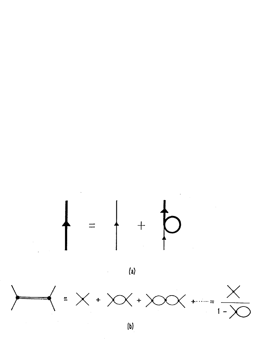
FIG. 1.: The two Schwinger-Dyson equations determining the dynamics of this model in the Hartree + RPA approximation: (a) the one-body, or “gap” equation; and (b) the two-body, or Bethe-Salpeter equation. The thin solid line is the bare, or “current” quark, the heavy solid line is the constituent quark and the double solid line is either the composite antisymmetric tensor-, or pseudo-tensor boson.

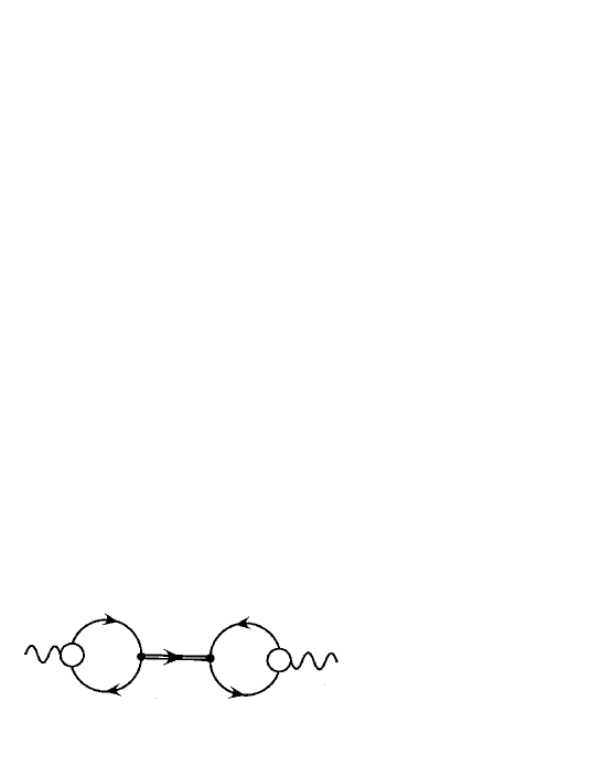
FIG. 2.: The vector current polarization tensor $\pi_{\mu\nu}$. The wavy lines are the Yang-Mills vector bosons, solid lines are constituent quarks and the double solid line is the antisymmetric pseudo-tensor boson.

REFERENCES

- [1] Y. Nambu, Phys. Rev. Lett. 4, 380 (1960); Y. Nambu and G. Jona-Lasinio, Phys. Rev. 122, 345 (1961); Phys. Rev. 124, 246 (1961). See also V. G. Vaks and A. I. Larkin, Sov. Phys. JETP 13, 192 (1961).
- [2] T. Eguchi and H. Sugawara, Phys. Rev. D 10, 4257 (1974), and T. Eguchi, Phys. Rev. D 14, 2755 (1976).
- [3] V.I. Ogievetskii and I.V. Polubarinov, Sov. J. Nucl. Phys. 4, 156 (1966).
- [4] M. Kalb and P. Ramond, Phys. Rev. D 9, 2273 (1974).
- [5] Y. Nambu, Phys. Rev. D 10, 4262 (1974).
- [6] V. Dmitrašinović, Phys. Rev. D 56, 247 (1997).
- [7] G. ‘t Hooft, Phys. Rev. D 14, 3432 (1976), (E) ibid. 18, 2199 (1978).
- [8] C. Itzykson and J. B. Zuber, Quantum Field Theory, (McGraw-Hill, New York, 1980).
- [9] V. Dmitrašinović, Phys. Lett. B 451, 170 (1999).
- [10] J. Schwinger, Phys. Rev. 125, 397 (1962), ibid. 128, 2425 (1962).
- [11] P. W. Higgs, Phys. Lett. 12, 132 (1964), Phys. Rev. Lett. 13, 508 (1964) and Phys. Rev. 145, 1156 (1966); F. Englert and R. Brout, Phys. Rev. Lett. 13, 321 (1964); G. S. Guralnik, C. R. Hagen and T. W. B. Kibble, Phys. Rev. Lett. 13, 585 (1964).
- [12] E.C.G. Stückelberg, Helv. Phys. Acta 11, 225 (1938); see also C. R. Hagen, Phys. Rev. D 19, 2367 (1979).
- [13] Y. Freundlich and D. Lurié, Nucl. Phys. B 19, 557 (1970).
- [14] G. Cvetič, Rev. Mod. Phys. 71, 513 (1999)
- [15] S. Klimt et al., Nucl. Phys. A 516 (1990) 429.