Non-BPS Dyons and Branes in the Dirac-Born-Infeld Theory

H.R. Christiansen   
Centro Brasileiro de Pesquisas Físicas, CBPF - DCP
Rua Dr. Xavier Sigaud 150, 22290-180 Rio de Janeiro, Brazil
 
N. Grandi
   F.A. Schaposnik   and G. Silva
Departamento de Física, Universidad Nacional de La Plata
C.C. 67, 1900 La Plata, Argentina
Associated with CICBA
Abstract

Non-BPS dyon solutions to D3-brane actions are constructed when one or more scalar fields describing transverse fluctuations of the brane, are considered. The picture emerging from such non-BPS configurations is analysed, in particular the response of the D-brane-string system to small perturbations.

La Plata-Th 99/13

I Introduction

Solutions to Dirac-Born-Infeld (DBI) theory have recently drawn much attention in connection to the dynamics of Dp-branes [1]-[15]. Indeed, the DBI action for $p+1$ dimensional gauge fields and a number of scalars describing transverse fluctuations of the brane allow static Bogomol’nyi-Prasad-Sommerfield (BPS) and non-BPS configurations, which can be interpreted in terms of branes and strings attached to them.

Although many (static) properties related to intersecting branes come from supersymmetry and BPS arguments, specific dynamical features depend strongly on the non-linearity of the DBI action. In particular, those related to the effective boundary conditions imposed to strings attached to branes must be investigated using the full DBI action. Moreover, non-BPS configurations might be useful for the study of certain non-perturbative aspects of field theories that describe the low energy dynamics of branes[16].

BPS and non-BPS (throat) purely electric solutions to DBI theory were constructed in [3]-[4]. Also the propagation of a perturbation normal to both the string and the 3-brane action was investigated in [3] for a BPS background. The results obtained show that the picture of a string attached to the brane with Dirichlet boundary conditions emerges naturally from DBI dynamics. In [8]-[9] perturbations polarized along the brane in a BPS background were studied and it was shown that Neumann boundary conditions are realized in this case.

Other purely electric non-BPS solutions to DBI action for the world volume gauge field and scalar fields were constructed in [6] where also magnetically charged BPS solutions were discussed. A detailed study of BPS dyonic solutions was presented later in [10].

In this paper we concentrate in the case of D3-branes and explicitly construct non-BPS dyon solutions when the U(1) gauge field couples to one or more scalar fields. We then analyse the solutions in connection with the geometry of the bending of the brane due to the tension of a $(n,m)$-string [17]-[18] carrying both electric and magnetic charges . Studying the energy of these non-BPS configurations, we compare the results with those obtained in the purely electric BPS and non-BPS cases [3]-[10]. We also study small excitations, transverse both to the brane and to the string, in order to test whether the response of the non-BPS solution is consistent with the interpretation in which the brane-string system described corresponds to the appropriate (Dirichlet) boundary condition.

The plan of the paper is as follows: in section II we construct the non-BPS solutions, with both electric and magnetic charges, to the DBI model for an Abelian gauge field in the world volume, coupled to one scalar. We discuss the properties of the solutions and compare them to other solutions already described in the literature. We also compute the renormalized energy and interpret the dyonic non-BPS solution in terms of strings attached to D3-branes. Then, in section III, we consider small perturbations to the non-BPS background, normal to the brane and to the string, in order to test the resulting boundary conditions. Finally, we summarize and discuss our results in section IV.

II Solutions of the Dirac-Born-Infeld Action

The D3-brane action in the static gauge takes the form

$$S=-T_{3}\int d^{4}x\sqrt{-{\rm det}(\eta_{\mu\nu}+T^{-1}F_{\mu\nu}+\partial_{\mu}X^{a}\partial_{\nu}X^{a})}$$ (1)

where $\eta_{\mu\nu}$ is Minkowski metric in $3+1$ dimensions, ${\rm diag}(\eta_{\mu\nu})=(-1,1,1,1)$, $F_{\mu\nu}$ is the world volume electromagnetic gauge field strength, $X^{a}$ are scalar fields ($a=4,5,\ldots,9$) which describe transverse fluctuations of the brane and

$$T_{3}=\frac{1}{2\pi g_{s}}T^{2}\,,\;\;\;T=\frac{1}{2\pi\alpha^{\prime}}$$ (2)

with $g_{s}$ the string coupling constant. This action can be obtained by dimensional reduction of a Born-Infeld action in 10 dimensional flat space-time ($x^{M}$, $M=0,1,2,\ldots,9$), assuming that the fields depend only on the first $1+3$ coordinates $x^{\mu}$ and that the extra components $A_{4},A_{5}\ldots A_{9}$ of the gauge field represent the scalar fields. We shall consider first the case in which there is just one excited scalar field, $X^{a}=\delta^{a9}X$. In this case eq.(1) takes the form

$\displaystyle S$ $\displaystyle=$ $\displaystyle-T_{3}\int d^{4}x\left(\left(1+\partial_{\mu}X\partial^{\mu}X\right)\left(1+\frac{1}{2T^{2}}F_{\mu\nu}F^{\mu\nu}\right)-\frac{1}{16T^{4}}\left(\tilde{F}_{\mu\nu}F^{\mu\nu}\right)^{2}\right.$ (4)
$\displaystyle\left.+\frac{1}{T^{2}}\partial^{\mu}XF_{\mu\nu}F^{\nu\rho}\partial_{\rho}X\right)^{1/2}$

The equations of motion for time-independent solutions read,

$\displaystyle\vec{\nabla}\cdot\left(\frac{1}{R}\left(\vec{\nabla}X+\frac{1}{T^{2}}(\vec{B}\cdot\vec{\nabla}X)\vec{B}+\frac{1}{T^{2}}\vec{E}\wedge(\vec{E}\wedge\vec{\nabla}X)\right)\right)=0$ (5)
$\displaystyle\vec{\nabla}\cdot\left(\frac{1}{R}\left(\vec{E}+\vec{\nabla}X\wedge(\vec{E}\wedge\vec{\nabla}X)+\frac{1}{T^{2}}(\vec{E}\cdot\vec{B})\vec{B}\right)\right)=0$ (6)
$\displaystyle\vec{\nabla}\wedge\left(\frac{1}{R}\left(\vec{B}+(\vec{B}\cdot\vec{\nabla}X)\vec{\nabla}X-\frac{1}{T^{2}}(\vec{E}\cdot\vec{B})\vec{E}\right)\right)=0$ (7)

Here, the $U(1)$ electric field $\vec{E}$ and magnetic induction $\vec{B}$ are defined as usual as

$$E_{i}=F_{i0}\;,\;\;\;B_{i}=\frac{1}{2}\varepsilon_{ijk}F_{jk}$$ (8)

Concerning $R$, it is defined as

$\displaystyle R^{2}$ $\displaystyle=$ $\displaystyle 1+(\vec{\nabla}X)^{2}+\frac{1}{T^{2}}\left(\vec{B}^{2}-\vec{E}^{2}+(\vec{B}\cdot\vec{\nabla}X)^{2}-(\vec{E}\wedge\vec{\nabla}X)^{2}\right)$ (10)
$\displaystyle-\frac{1}{T^{4}}(\vec{E}\cdot\vec{B})^{2}$

Now, since we are interested in bion solutions [3]-[4] carrying both electric $q_{e}$ and magnetic $q_{m}$ charges, this necessarily implies that $\vec{E}$ and $\vec{B}$ have delta function sources (c.f. [19] where dyon configurations with an extended magnetic source are constructed). For the case $X=0$ one easily finds such a solution to (7) in the form

$$A_{0}=-\frac{q_{e}}{4\pi}\int_{r}^{\infty}dr\frac{1}{\sqrt{(q_{e}^{2}+q_{m}^{2})(4\pi T)^{-2}+r^{4}}}$$ (11)
$$A_{\varphi}=\frac{q_{m}}{4\pi r}\frac{(1-\cos\theta)}{\sin\theta}\;,\;\;\;A_{\theta}=A_{r}=0$$ (12)

This solution can be obtained from the purely electric Born-Infeld one by a duality rotation [20].

Following [4]-[6] , we construct the general solution by performing a boost (in $10$ dimensional space) in the $x^{9}$ direction leading to

$\displaystyle X$ $\displaystyle=$ $\displaystyle-\frac{q_{e}\sqrt{a}}{4\pi T}\int_{r}^{\infty}dr\frac{1}{\sqrt{r^{4}_{0}+r^{4}}}$ (13)
$\displaystyle A_{0}$ $\displaystyle=$ $\displaystyle-\frac{q_{e}}{4\pi}\int_{r}^{\infty}dr\frac{1}{\sqrt{r_{0}^{4}+r^{4}}}$ (14)
$\displaystyle A_{\varphi}$ $\displaystyle=$ $\displaystyle\frac{q_{m}}{4\pi r}\frac{(1-\cos\theta)}{\sin\theta}\;,\;\;\;A_{\theta}=A_{r}=0$ (15)

where

$$r_{0}^{4}=(4\pi T)^{-2}((1-a)q_{e}^{2}+q_{m}^{2})$$ (16)

and $a$ is related to the square of the boost velocity. The electric and magnetic fields associated with (15) take the form

$\displaystyle\vec{E}$ $\displaystyle=$ $\displaystyle\frac{q_{e}}{4\pi\sqrt{r_{0}^{4}+r^{4}}}\check{r}$ (17)
$\displaystyle\vec{B}$ $\displaystyle=$ $\displaystyle\frac{q_{m}}{4\pi r^{2}}\check{r}$ (18)

Note that since the boost is in the $x^{9}$ direction, it does not affect the transverse $x^{i}\,,i=1,2,\ldots,8$ directions. Moreover, since we are considering static solutions, $A_{\varphi}$ in (15) is not affected and the magnetic field remains unchanged by the boost.

These solutions generalize all known (one source) solutions already discussed in the DBI-brane context, either the BPS or non-BPS ones. Setting $q_{m}=0$ we recover, for $a<1$, the electric bions, for $a>1$, the electric throat/catenoid solutions and, for $a=1$, the electric BPS solution [3]-[6]. The new solutions we have found generalize these electric bions and throats to dyonic ones.

Concerning the magnetic field $\vec{B}$, it is important to note that its value is $a$ independent and has the usual Dirac monopole functional form corresponding to a quantized magnetic charge. Indeed, the magnetic induction $\vec{H}$ is given by

$$\vec{H}\equiv\frac{1}{R}\left(\vec{B}+\left(\vec{B}\cdot\vec{\nabla}X\right)\vec{\nabla}X-\frac{1}{T^{2}}\left(\vec{E}\cdot\vec{B}\right)\vec{E}\right)=\frac{q_{m}}{4\pi\sqrt{r_{0}^{4}+r^{4}}}\check{r}$$ (19)

The electric and magnetic charges of the solutions were adjusted so that

$$\int_{S_{\infty}}dS_{i}E^{i}=q_{e}\,,\;\;\;\;\;\;\;\;\int_{S_{\infty}}dS_{i}B^{i}=q_{m}$$ (20)

It is useful to define the scalar field charge $q_{s}$ in the form

$$q_{s}\equiv T\int_{S_{\infty}}dS_{i}\partial^{i}X=\sqrt{a}\,q_{e}$$ (21)

In terms of charges, $r_{0}$ in (16) takes the form

$$r_{0}^{4}=(4\pi T)^{-2}\left(q_{e}^{2}+q_{m}^{2}-q_{s}^{2}\right)$$ (22)

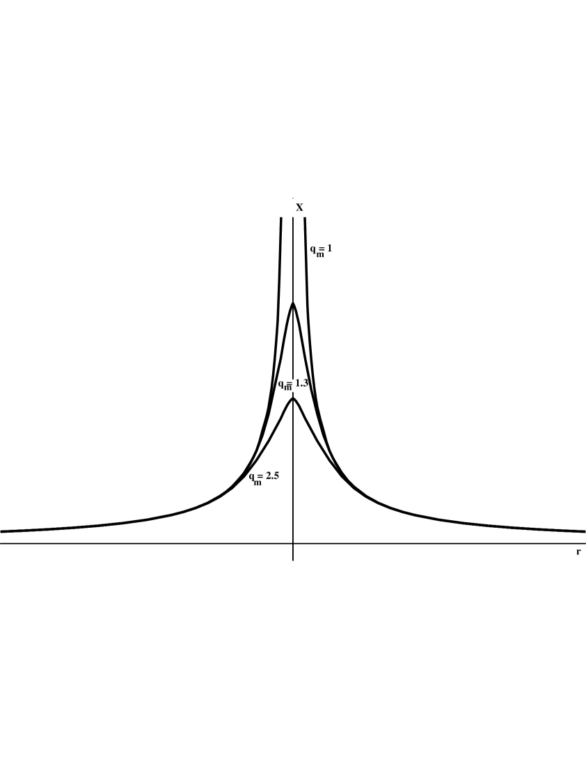
From (15) one can see that, in the range $q_{s}^{2}\leq q_{m}^{2}+q_{e}^{2}$, the scalar takes essentially the form depicted in Fig. 1. Qualitatively, its behavior is similar to the purely electric solution found in [6] except that the existence of a non-zero magnetic charge lowers the height of the cusp.

For $q_{s}^{2}>q_{e}^{2}+q_{m}^{2}$ the scalar takes the form of the solution depicted in Fig. 2 which can be viewed as two asymptotically flat branes (in fact, a brane-antibrane pair) joined by a throat of radius $r_{t}$. These branes are separated a distance $\Delta=2|X(r_{t})|$ which corresponds to the difference between the two asymptotic values of $X(r)$. The radius of the throat is given by

$$r_{t}^{4}=-r_{0}^{4}=(4\pi T)^{-2}\left(q_{s}^{2}-q_{e}^{2}-q_{m}^{2}\right)$$ (23)

Note that increasing the magnetic charge makes the throat slimmer and $\Delta$ larger.

BPS solutions correspond to the case $r_{0}=0$. That is, when the scalar charge satisfies

$$q_{s}^{BPS}=\pm\sqrt{q_{e}^{2}+q_{m}^{2}}$$ (24)

When (24) holds, the solutions satisfying Bogomol’nyi equations

$\displaystyle\vec{E}$ $\displaystyle=$ $\displaystyle T\cos\xi\vec{\nabla}X$ (25)
$\displaystyle\vec{B}$ $\displaystyle=$ $\displaystyle T\sin\xi\vec{\nabla}X$ (26)

are

$\displaystyle X$ $\displaystyle=$ $\displaystyle-\frac{\sqrt{q_{e}^{2}+q_{m}^{2}}}{4\pi Tr}$ (27)
$\displaystyle\vec{E}$ $\displaystyle=$ $\displaystyle\frac{q_{e}}{4\pi r^{2}}\check{r}$ (28)
$\displaystyle\vec{B}$ $\displaystyle=$ $\displaystyle\frac{q_{m}}{4\pi r^{2}}\check{r}$ (29)

with

$\displaystyle\cos\xi=\frac{q_{e}}{\sqrt{q_{e}^{2}+q_{m}^{2}}}$ (30)

Note that $r_{0}=0$ implies that the boost parameter $a=1+q_{m}^{2}/q_{e}^{2}>1$. In particular, for $q_{m}=0$ the boost is a light-cone one. In fact, $q_{m}=0$ corresponds to $\xi=0$ and then (15) reduces to the electric BPS solution discussed in [3]-[4]. The choice $\xi=\pi/2$ ($q_{e}=0$) corresponds to the magnetic BPS solution discussed in [4]. For arbitrary $\xi$ our BPS solution coincides with that analysed in [10].

Let us now compute the static energy for the non-BPS configurations described earlier and relate it to the bending of branes. We consider the case in which there is only one D3-brane and first compute the energy stored in the world volume of the brane for the configuration (15)-(18) with $r_{0}^{4}\geq 0$,

$\displaystyle E_{wv}$ $\displaystyle=$ $\displaystyle\int d^{3}x\,T_{00}$ (31)
$\displaystyle=$ $\displaystyle\frac{2}{g_{s}}\int r^{2}dr\left(\frac{q_{e}^{2}+q_{m}^{2}}{(4\pi r)^{2}\sqrt{r^{4}+r_{0}^{4}}}+T^{2}\left(\frac{r^{2}}{\sqrt{r^{4}+r_{0}^{4}}}-1\right)\right)$ (32)
$\displaystyle=$ $\displaystyle\frac{\Gamma^{2}(1/4)}{96\pi^{5/2}g_{s}}\left({2}(q_{e}^{2}+q_{m}^{2})+q_{s}^{2}\right)\frac{1}{r_{0}}$ (33)

Since the BPS limit is reached when $r_{0}=0$, we see that $E_{wv}$ diverges precisely at the point which should correspond to the lower bound for the energy. In order to avoid this problem, one can normalize the energy with respect to the Bogomol’nyi value. To this end we define

$\displaystyle E$ $\displaystyle=$ $\displaystyle E_{wv}-E_{sub}=E_{wv}-\frac{\Gamma^{2}(1/4)}{32\pi^{5/2}g_{s}}|q_{s}|\sqrt{q_{e}^{2}+q_{m}^{2}}\frac{1}{r_{0}}$ (34)
$\displaystyle=$ $\displaystyle\frac{\Gamma^{2}(1/4)}{6\sqrt{\pi}g_{s}}T^{2}\left(2-\frac{3|q_{s}|}{|q_{s}|+\sqrt{q_{e}^{2}+q_{m}^{2}}}\right)r_{0}^{3}$ (35)

Clearly, $E=0$ in the BPS case ($r_{0}=0$). In general, $0\leq E<\infty$ and then the BPS configuration gives the lower bound for the energy. We show in Fig. 3 the energy as given by (35) as a function of the scalar charge. At fixed electric charge, one can see that, as the magnetic charge grows, the Bogomol’nyi bound is attained for larger scalar charge.

The subtraction performed in (35) can be interpreted as follows. Using eq.(15), $E_{wv}$, as given by eq.(33), can be written as

$$E_{wv}=\frac{T}{6\pi g_{s}}\frac{1}{|q_{s}|}\left(2(q_{e}^{2}+q_{m}^{2})+q_{s}^{2}\right)\,|X(0)|$$ (36)

Concerning the subtracted term, it takes the form

$$E_{sub}=\frac{T}{2\pi g_{s}}\sqrt{q_{e}^{2}+q_{m}^{2}}\,|X(0)|$$ (37)

The connection between the dyon electric field and fundamental strings leads to the quantization of the electric flux [3] so that $q_{e}=2\pi g_{s}n$. For the magnetic charge, we write $q_{m}=2\pi m$. Then, $E_{sub}$ can be rewritten in the form

$$E_{sub}=T\sqrt{n^{2}+\frac{1}{g_{s}^{2}}m^{2}}|X(0)|$$ (38)

The renormalized energy $E$ as defined in (35) can then be written as

$\displaystyle E$ $\displaystyle=$ $\displaystyle E_{wv}-T_{(n,m)}\int_{0}^{|X(0)|}dX$ (39)
$\displaystyle=$ $\displaystyle E_{wv}+T_{(n,m)}\int_{|X(0)|}^{\infty}dX-T_{(n,m)}\int_{0}^{\infty}dX$ (40)

where

$$T_{(n,m)}=T\sqrt{n^{2}+\frac{1}{g_{s}^{2}}m^{2}}$$ (41)

Formula (40) makes clear the rationale of the subtraction: the second term in the r.h.s. of (40) represents the energy of a semi-infinite string (with tension $T_{(n,m)}$) extending from the cusp of the spike to infinity. The third term subtracts the infinite energy of a string extending from 00 (from a flat brane) to infinity. We are then computing the energy of a brane pulled by a string with respect to the energy of a non-interacting configuration brane+string (which turns to be a BPS solution).

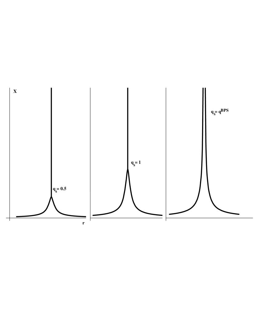
We represent in figure 4 a sequence of growing spikes as the scalar charge increases up to the point it attains its BPS value $q_{s}^{BPS}$.

One can also compute the static energy stored in the worldvolume for the throat solution ($r_{t}^{2}=-r_{0}^{2}>0$). One gets

$$E_{wv}=\frac{\Gamma^{2}(1/4)}{48\sqrt{2}\pi^{5/2}g_{s}}\left({2}(q_{e}^{2}+q_{m}^{2})+q_{s}^{2}\right)\frac{1}{r_{t}}+\frac{4}{3}\frac{T^{2}}{g_{s}}r_{t}^{3}$$ (42)

which also diverges in the BPS ($r_{t}\to 0$) limit. The adequate subtraction now required in order to get a finite result is

$$E_{sub}=\frac{\Gamma^{2}(1/4)}{16\sqrt{2}\pi^{5/2}g_{s}}|q_{s}|\sqrt{q_{e}^{2}+q_{m}^{2}}\frac{1}{r_{t}}$$ (43)

We then have for the throat

$$E=E_{wv}-E_{sub}=\frac{4}{3}\frac{T^{2}}{g_{s}}\left(1+\frac{\Gamma^{2}(1/4)}{4\sqrt{2\pi}}\frac{|q_{s}|-2\sqrt{q_{e}^{2}+q_{m}^{2}}}{|q_{s}|+\sqrt{q_{e}^{2}+q_{m}^{2}}}\right)r_{t}^{3}$$ (44)

The subtracted energy $E_{sub}$ defined by eq.(43) can be written as

$$E_{sub}=\frac{T}{2\pi g_{s}}\sqrt{q_{e}^{2}+q_{m}^{2}}2|X(r_{t})|=T_{(n,m)}\Delta$$ (45)

where $T_{(n,m)}$ is defined by eq.(41). Then, the finite energy $E$ in (44) corresponds to the difference between the throat solution and a non-interacting configuration brane-string-antibrane.

We shall now briefly describe non-BPS solutions of the DBI action when two scalar fields are present. Starting from action (1) with $X^{8}=X$ and $X^{9}=Y$, the corresponding equations of motion read

$\displaystyle\vec{\nabla}\cdot\left(\frac{1}{R}\left(\vec{\nabla}X+(\vec{\nabla}X\wedge\vec{\nabla}Y)\wedge\vec{\nabla}Y-\frac{1}{T^{2}}\vec{E}\cdot(\vec{\nabla}X\wedge\vec{\nabla}Y)(\vec{E}\wedge\vec{\nabla}Y)\right.\right.$ (46)
$\displaystyle\left.\left.+\frac{1}{T^{2}}(\vec{B}\cdot\vec{\nabla}X)\vec{B}+\frac{1}{T^{2}}\vec{E}\wedge(\vec{E}\wedge\vec{\nabla}X)\right)\right)=0$ (47)
$\displaystyle\vec{\nabla}\cdot\left(\frac{1}{R}\left(\vec{\nabla}Y+(\vec{\nabla}Y\wedge\vec{\nabla}X)\wedge\vec{\nabla}X-\frac{1}{T^{2}}\vec{E}\cdot(\vec{\nabla}Y\wedge\vec{\nabla}X)(\vec{E}\wedge\vec{\nabla}X)\right.\right.$ (48)
$\displaystyle\left.\left.+\frac{1}{T^{2}}(\vec{B}\cdot\vec{\nabla}Y)\vec{B}+\frac{1}{T^{2}}\vec{E}\wedge(\vec{E}\wedge\vec{\nabla}Y)\right)\right)=0$ (49)
$\displaystyle\vec{\nabla}\cdot\left(\frac{1}{R}\left(\phantom{\frac{1}{T^{5}}}\!\!\!\!\!\!\!\!\vec{E}+\vec{\nabla}X\wedge(\vec{E}\wedge\vec{\nabla}X)+\vec{\nabla}Y\wedge(\vec{E}\wedge\vec{\nabla}Y)\right.\right.$ (50)
$\displaystyle\left.\left.+\vec{E}\cdot(\vec{\nabla}Y\wedge\vec{\nabla}X)(\vec{\nabla}Y\wedge\vec{\nabla}X)-\frac{1}{T^{2}}(\vec{E}\cdot\vec{B})\vec{B}\right)\right)=0$ (51)
$\displaystyle\vec{\nabla}\wedge\left(\frac{1}{R}\left(\vec{B}+(\vec{B}\cdot\vec{\nabla}X)\vec{\nabla}X+(\vec{B}\cdot\vec{\nabla}Y)\vec{\nabla}Y-\frac{1}{T^{2}}(\vec{E}\cdot\vec{B})\vec{E}\right)\right)=0$ (52)
(53)

where $R$ is now given by

$\displaystyle R^{2}$ $\displaystyle=$ $\displaystyle 1+(\vec{\nabla}X)^{2}+(\vec{\nabla}Y)^{2}+\left(\vec{\nabla}X\wedge\vec{\nabla}Y\right)^{2}+\frac{1}{T^{2}}\left(\vec{B}^{2}-\vec{E}^{2}\right.$ (56)
$\displaystyle\left.+(\vec{B}\cdot\vec{\nabla}X)^{2}-(\vec{E}\wedge\vec{\nabla}X)^{2}+(\vec{B}\cdot\vec{\nabla}Y)^{2}-(\vec{E}\wedge\vec{\nabla}Y)^{2}\right.$
$\displaystyle\left.-(\vec{E}\cdot(\nabla X\wedge\vec{\nabla}Y))^{2}\right)-\frac{1}{T^{4}}(\vec{E}\cdot\vec{B})^{2}$

The solution takes the form

$\displaystyle\vec{\nabla}X$ $\displaystyle=$ $\displaystyle({q_{s}^{8}}/{Tq_{e}})\vec{E}$ (57)
$\displaystyle\,\vec{\nabla}Y$ $\displaystyle=$ $\displaystyle({q_{s}^{9}}/{Tq_{e}})\vec{E}$ (58)
$\displaystyle\vec{E}$ $\displaystyle=$ $\displaystyle\frac{q_{e}}{4\pi\sqrt{r_{0}^{4}+r^{4}}}\check{r}$ (59)
$\displaystyle\vec{B}$ $\displaystyle=$ $\displaystyle\frac{q_{m}}{4\pi r^{2}}\check{r}$ (60)

where $q_{s}^{8}$ and $q_{s}^{9}$ are the charges of the two scalars, defined as in (21),

$$q_{s}^{a}\equiv T\int_{S_{\infty}}dS_{i}\partial^{i}X^{a}$$ (61)

and $r_{0}$ is now given by

$$r_{0}^{4}=q_{e}^{2}+q_{m}^{2}-\left(q_{s}^{8}\right)^{2}-\left(q_{s}^{8}\right)^{2}$$ (62)

This non-BPS solution can be interpreted as a spike that extends in the direction $q_{s}^{8}\check{e}^{8}+q_{s}^{9}\check{e}^{9}$, with $\check{e}^{8}$ ($\check{e}^{9}$) denoting the unit vector in the $X^{8}$ ($X^{9}$) directions. It is interesting to note that there is a family of values for the scalar charges $({q_{s}^{8}}^{BPS},{q_{s}^{9}}^{BPS})$ which leads to the BPS limit,

$$\left({q_{s}^{8}}^{BPS}\right)^{2}+\left({q_{s}^{9}}^{BPS}\right)^{2}=q_{e}^{2}+q_{m}^{2}$$ (63)

The particular solution ${q_{s}^{8}}^{BPS}=q_{e}$ and ${q_{s}^{9}}^{BPS}=q_{m}$ corresponds to the BPS configuration with a $\nu=1/4$ fraction of unbroken supersymmetry analysed in [10], which solves

$$\vec{E}=T\vec{\nabla}X\,,\;\;\;\vec{B}=T\vec{\nabla}Y$$ (64)

It is interesting to note that eqs.(64) exhibit an invariance under transformations which correspond to a duality rotation for the electric and magnetic fields and a related $SO(2)$ rotation for the scalar fields. Indeed, the transformation

$\displaystyle\vec{E}+i\vec{B}$ $\displaystyle\longrightarrow$ $\displaystyle\exp(i\theta)(\vec{E}+i\vec{B})$ (65)
$\displaystyle X+iY$ $\displaystyle\longrightarrow$ $\displaystyle\exp(i\theta)(X+iY)$ (66)

Other solutions of eq.(63) are those that correpond to $\nu=1/2$, which can be obtained by an $SO(2)$ rotation of (29) in the $(X^{8},X^{9})$ plane.

III Dynamics and Boundary Conditions

We shall now analyse the response of the theory to small fluctuation around the static non-BPS dyon solutions that we have found above, in the spirit of ref.[3].

We take as a background the non-BPS spike solution (15) and study the propagation of a $s$-wave perturbation $\eta$, polarized in a direction perpendicular to the brane and to $\check{X}^{9}$, say $\check{X}^{8}$. Starting from action (1), one obtains the linearized fluctuation equation around the static solution

$$-\left(r^{4}+\frac{q_{e}^{2}+q_{m}^{2}}{(4\pi T)^{2}}\right)\ddot{\eta}(r,t)+2r^{3}\eta^{\prime}(r,t)+\left(r^{4}+r_{0}^{4}\right)\eta^{\prime\prime}(r,t)=0$$ (67)

Writing $\eta(r,t)=\eta(r)\exp(i\omega t)$ and defining $x=\omega r$ the corresponding stationary equation is given by

$$\frac{1}{x^{2}}f(x)(x^{2}f(x)\eta^{\prime}(x))^{\prime}+\frac{\kappa^{2}+x^{4}}{x^{4}}\eta(x)=0$$ (68)

where

$$\kappa=\frac{\sqrt{q_{e}^{2}+q_{m}^{2}}}{4\pi T}\omega^{2}$$ (69)

and

$$f(x)=\frac{\sqrt{x^{4}+\omega^{4}r_{0}^{4}}}{x^{2}}$$ (70)

In the BPS limit ($r_{0}\to 0$) $f(x)\to 1$ and we recover the case discussed originally in [3],[8].

To study eq.(68) we change from $x$ to a new variable $\xi$ which measures the length along $X$

$$\xi(r)=\omega\int_{\sqrt{\kappa}/\omega}^{r}d\tilde{r}\sqrt{1+{X^{\prime}}^{2}(\tilde{r})}$$ (71)

Using the explicit form for the $X$ solution as given in (15), $\xi$ can be written in the form

$$\xi(x)=\int_{\sqrt{\kappa}}^{x}dy\sqrt{\frac{y^{4}+\kappa^{2}}{y^{4}+r_{0}^{4}\omega^{4}}}$$ (72)

Defining

$$\tilde{\eta}(x)=\left(x^{4}+{\kappa^{2}}\right)^{\frac{1}{4}}\eta(x)$$ (73)

eq.(68) becomes a one-dimensional Schrödinger equation

$$\left(-\frac{d^{2}}{d\xi^{2}}+V(\xi)\right)\tilde{\eta}(\xi)=\tilde{\eta}(\xi)$$ (74)

with potential

$$V(\xi)=\frac{5\kappa^{2}x^{6}}{\left(x^{4}+\kappa^{2}\right)^{3}}+\frac{(4\pi T)^{2}}{q_{e}^{2}+q_{m}^{2}}r_{0}^{4}\kappa^{2}x^{2}\frac{3\kappa^{2}-2x^{4}}{\left(\kappa^{2}+x^{4}\right)^{3}}$$ (75)

The first term in (75) is formally identical to the potential in the BPS limit [3] except that the relation between $\xi$ and $x$, given by (72) depends on $r_{0}$ and hence only coincides with the BPS answer for $r_{0}=0$. Another important difference with the BPS case concerns the one dimensional domain in which potential (75) is defined: being our solution a non-BPS one, $\xi$ extends from a finite (negative) $\xi(0)$ to $+\infty$, since the cusp for this solution has a finite height $X(0)$. Now, from $X^{9}=X(0)$ to infinity (i.e., in the $\xi$-interval $(-\infty,\xi(0))$) the disturbance just acts on the free scalar action of the semi-infinite string attached to the brane. Then, in this region, one has, instead of (74),

$$-\frac{d^{2}\tilde{\eta}(\xi)}{d\xi^{2}}=\tilde{\eta}(\xi)$$ (76)

We can then consider eq.(74) in the whole one dimensional domain by defining

$$V_{eff}(\xi)=\left\{\begin{array}[]{ll}0&\mbox{if $-\infty<\xi<\xi(0)$}\\ V(\xi)&\mbox{if $\xi(0)<\xi<\infty$}\end{array}\right.$$ (77)

Potential (77), corresponding to a non-BPS disturbed configuration, is more involved than the BPS one, which was originally studied in the $\kappa\to 0$ limit using delta function and square barrier approximations [3],[8]. We shall take this second way and approximate the potential by a rectangular potential, adjusting its height and width so that the integral of $V$ and the integral of $\sqrt{V}$ coincide. We then define

$$S=\int\sqrt{V(\xi)}d\xi\,,\;\;\;\;U=\sqrt{\kappa}\int V(\xi)d\xi$$ (78)

One can see, by an appropriate change of variables that neither $S$ nor $U$ depend on $\kappa$. In terms of these quantities, one finds for the reflection and transmission amplitudes

$\displaystyle R$ $\displaystyle=$ $\displaystyle\frac{\exp\left(-i\sqrt{\kappa}S^{2}/U\right)}{-1+({2i\sqrt{\kappa}S}/{U}){\rm coth}S}$ (79)
$\displaystyle T$ $\displaystyle=$ $\displaystyle i\left(\frac{2\sqrt{\kappa}S}{U}{\rm cosech}S\right)R$ (80)

Eq. (80) shows that one has complete reflection with a phase-shift approaching $\pi$ in the low-energy limit ($\kappa\to 0$). Computing numerically $S$ and $U$ one can also see that the non-BPS reflection coefficient $|R(r_{0})|$ is slightly larger than the BPS one, $|R(r_{0})|>|R(0)|$.

We thus conclude from the analysis above that a transverse disturbance on the string attached to the non-BPS brane, reflects in agreement with the expected result for Dirichlet boundary conditions: the reflection amplitude $R$ goes to $-1$ in the low-energy ($\kappa\to 0$) limit. In the opposite limit ($\kappa\to\infty$) the potential vanishes so that the system passes from perfectly reflecting to perfectly transparent at a scale that, for the dyon background that we studied corresponds to $8\kappa\sim 5+r_{0}^{4}(4\pi T)^{2}/(q_{e}^{2}+q_{m}^{2})$. The emerging picture is then in agreement with the D3-brane acting as a boundary for open strings.

IV Summary and discussion

In summary we have constructed dyonic non-BPS solutions to the Dirac-Born-Infeld action for a U(1) gauge field in the world volume coupled to one or two scalars and analysed them in the context of brane dynamics. Although our solutions also include those BPS ones already discussed in the literature, we have concentrated on the non-BPS sector to test whether this characteristic affects the picture of strings attached to branes. One important quantity in the analysis of the non-BPS solutions is the value of the scalar charge $q_{s}$ which can be written in terms of the electric and magnetic charge as

$$q_{s}^{2}=q_{e}^{2}+q_{m}^{2}-(4\pi T)^{2}r_{0}^{4}$$ (81)

For $r_{0}^{4}>0$ our solutions correspond to a brane with a spike while for $r_{0}^{4}<0$ one has a brane-antibrane solution with a throat. The subtracted (renormalized) energy of these non-BPS dyon solutions can be arranged in a way that naturally leads to this picture of a brane pulled by a string with a tension $T_{(n,m)}=T\sqrt{n^{2}+m^{2}/g_{s}^{2}}$ ($m$ and $n$ being the number of magnetic and electric flux units of the solution). As shown graphically in Fig.4, as the scalar charge increases towards its BPS value $q_{s}^{BPS}$, the spike grows and then, once $q_{s}^{BPS}$ is exceeded, the solution becomes a pair of brane-antibrane joined by a throat. Solutions with two scalars can be constructed following analogous steps and also be interpreted in terms of spikes extending in the combined direction of the two scalars.

Finally we have studied the effect of small disturbances transverse both the string and the non-BPS brane showing through a scattering analysis that the results corresponds to the expected Dirichlet boundary conditions. In particular, the reflection amplitude for the non-BPS background is slighty larger than the result for the BPS case and tends to $-1$ in the low-energy limit.

Acknowledgements

This work is partially supported by CICBA, CONICET (PIP 4330/96), ANPCYT (PICT 97/2285), Argentina. N. Grandi is partially supported by a CICBA fellowship. G.  Silva is supported by a CONICET fellowship. H.R. Christiansen acknowledges partial support from FAPERJ, Fundaç ao de Amparo à Pesquisa do Rio de Janeiro, Brazil.

Refer to caption

FIG. 1.: The scalar $X$ as a function of $r$ for fixed electric charge $q_{e}=1$ and different values of the magnetic charge $q_{m}$. The value $q_{m}^{BPS}=1$ is the one for which the BPS limit is attained when $q_{e}=1$ and $q_{s}=\sqrt{2}$.

Refer to caption

FIG. 2.: The scalar $X$ as a function of $r$ for fixed electric charge $q_{e}=1$ and different values of the magnetic charge $q_{m}$. The value $q_{m}^{BPS}=1$ is the one for which the BPS limit is attained when $q_{e}=1$ and $q_{s}=\sqrt{2}$.

Refer to caption

FIG. 3.: The energy of the non-BPS configuration (a bent brane with an attached string) as a function of $a=q_{s}^{2}/q_{e}^{2}$ for different values of the magnetic charge $q_{m}$.

Refer to caption

FIG. 4.: The spike in the brane, pulled by the string, as a function of $r$ for values of the scalar charge (in appropriate units) going from $q_{s}=0.5$ (left) to the BPS value $q_{s}^{BPS}=\sqrt{q_{e}^{2}+q_{m}^{2}}=\sqrt{2}$ (right).

REFERENCES

  • [1] J. Polchinski, Phys. Rev. Lett. 75 (1995) 4724.
  • [2] See J. Polchinski, Tasi Lectures on D-Branes, hep-th/9611050 and references therein.
  • [3] C. Callan and J.M. Maldacena, Nucl.Phys. B513 (1998) 198
  • [4] G.W. Gibbons, Nucl. Phys. B514 (1998) 603.
  • [5] J.P. Gauntlett, J. Gomis and P.K. Townsend, JHEP 01 (1998) 003.
  • [6] A. Hashimoto, Phys.Rev. D57 (1998) 6441.
  • [7] D. Brecher, Phys. Lett. B442 (1998) 117.
  • [8] G.K. Savvidy, hep-th/9810163.
  • [9] C.G. Savvidy and K.G. Savvidy, hep-th/9902023.
  • [10] D. Bak, J. Lee and H. Min, Phys.Rev. D59 (1999) 045011.
  • [11] K. Hashimoto, JEPTH 07 (1999) 016.
  • [12] J.P. Gauntlett, C. Koehl, D. Mateos, P.K. Townsend and M. Zamblar, Phys. Rev. D60 (1999) 04504.
  • [13] G.W. Gibbons, Class.Quant.Grav. 16 (1999) 1471.
  • [14] G.W. Gibbons Lecture at 6th Conference on Quantum Mechanics of Fundamental Systems, Chile, 1997, hep-th/9801106.
  • [15] A.A. Tseytlin, to appear in the Yuri Golfand memorial volume ed. M. Shifman, Wd. Sci. , 2000, hep-th/9908105.
  • [16] O. Bergman and M.R. Gaberdiel, hep-th/9908126.
  • [17] J.H. Schwarz, Phys.Lett. B360 (1995) 13.
  • [18] E. Witten, Nucl. Phys. B460 (1996) 335.
  • [19] K. Ghoroku and K. Kaneko, hep-th/9908154.
  • [20] G. Gibbons and D.A. Rasheed, Nucl. Phys. B454 (1995) 185.