Qualitative Analysis of Isotropic Curvature String Cosmologies

Andrew P. Billyard^1a, Alan A. Coley^1,2b & James E. Lidsey^3c

¹Department of Physics,
Dalhousie University, Halifax, NS, B3H 3J5, Canada

²Department of Mathematics and Statistics,
Dalhousie University, Halifax, NS, B3H 3J5, Canada

³Astronomy Unit, School of Mathematical Sciences,
Queen Mary and Westfield, Mile End Road, London, E1 4NS, U. K.

A complete qualitative study of the dynamics of string cosmologies is presented for the class of isotopic curvature universes. These models are of Bianchi types I, V and IX and reduce to the general class of Friedmann–Robertson–Walker universes in the limit of vanishing shear isotropy. A non–trivial two–form potential and cosmological constant terms are included in the system. In general, the two–form potential and spatial curvature terms are only dynamically important at intermediate stages of the evolution. In many of the models, the cosmological constant is important asymptotically and anisotropy becomes dynamically negligible. There also exist bouncing cosmologies.

PACS NUMBERS: 98.80.Cq, 04.50+h, 98.80.Hw

^aElectronic mail: jaf@mscs.dal.ca

^bElectronic mail: aac@mscs.dal.ca

^cElectronic mail: jel@maths.qmw.ac.uk

1 Introduction

One of the strongest constraints that a unified theory of the fundamental interactions must satisfy is that it leads to realistic cosmological models. There are known to be five consistent perturbative superstring theories in ten dimensions. (See, e.g., Ref. [1]). The type II and heterotic theories each contain a Neveu–Schwarz/Neveu–Schwarz (NS–NS) sector of bosonic massless excitations that includes a scalar dilaton field, a graviton and an antisymmetric two–form potential. The interactions between these fields lead to significant deviations from the standard, hot big bang model based on conventional Einstein gravity [3] and a study of the cosmological consequences of superstring theory is therefore important.

In string cosmology, the dynamics of the universe below the string scale is determined by the effective supergravity actions. The NS–NS string cosmologies contain the non–trivial fields discussed above. Recently [4] (hereafter referred to as paper I), a complete qualitative analysis for the spatially flat Friedmann–Robertson–Walker (FRW) and axisymmetric Bianchi type I NS–NS string cosmologies was presented. A central charge deficit was also included and found to have significant effects on the nature of the equilibrium points. This study unified and extended previous qualitative analyses of this system [6, 7, 8].

In Ref. [5] (hereafter referred to as paper II), a phenomenological cosmological constant was introduced into the string frame effective action in such a way that it was not coupled directly to the dilaton field. Such a term yields valuable insight into the dynamics of more general string models containing non–trivial Ramond–Ramond (RR) fields. The interplay between such a cosmological constant and the two–form potential had not been considered previously. It was found that the interactions led to heteroclinic orbits in the phase space, where the universe underwent a series of oscillations between expanding and contracting phases.

The purpose of the present paper is to extend the work of [4, 5] to both isotropic and anisotropic cosmologies containing spatial curvature terms. In particular, we consider the class of ‘isotropic curvature’ universes [9, 10]. These are spatially homogeneous but contain non-trivial curvature and anisotropy. The characteristic feature of these models is that the three-dimensional Ricci curvature tensor is isotropic. In other words, ${{}^{(3)}}R_{ij}$ is proportional to $k\delta_{ij}$ on the spatial hypersurfaces and these surfaces therefore have constant curvature $k$ [9]. The class of isotropic curvature universes contains the Bianchi type I ($k=0$) and V ($k<0$) models and a special case of the Bianchi type IX ($k>0$) models [10].

The four–dimensional line element of these cosmologies is given by [9, 10]

$$ds^{2}=-dt^{2}+e^{2\alpha(t)}\left[\left(\mathbf{\omega}^{1}\right)^{2}+e^{-2\sqrt{3}\beta_{s}(t)}\left(\mathbf{\omega}^{2}\right)^{2}+e^{2\sqrt{3}\beta_{s}(t)}\left(\mathbf{\omega}^{3}\right)^{2}\right],$$ (1.1)

where the one-forms $\{\omega^{1},\omega^{2},\omega^{3}\}$ are given in [9, 10]. The spatial hypersurfaces, $t={\rm constant}$, are the surfaces of homogeneity. The variable, $\alpha$, parametrizes the effective spatial volume of the universe and $\beta$ determines the level of anisotropy. We refer to it as the shear parameter. In essence, the isotropic curvature models can be regarded as the simplest anisotropic generalizations of the flat $(k=0)$, open $(k<0)$ and closed $(k>0)$ FRW universes, respectively. The isotropic models are recovered when $\dot{\beta}=0$.

The paper is organized as follows. In Section 2, we summarize the form of the effective actions we consider. The cosmological field equations are derived and the general asymptotic behaviour of the two–form potential and spatial curvature is discussed. The global qualitative dynamics for the different classes of models is determined in Sections 3 and 4. We summarize and conclude our results in Section 5. The functional forms of the equilibrium points that arise in the analysis are presented in the Appendix.

2 Cosmological Field Equations

2.1 String Effective Action

The NS–NS sector of massless bosonic excitations is common to both the type II and heterotic superstring theories. The four–dimensional, string effective action for the NS–NS fields can be written as [15]

$$S=\int d^{4}x\sqrt{-g}e^{-\Phi}\left[R+\left(\nabla\Phi\right)^{2}-\frac{1}{12}H_{\mu\nu\lambda}H^{\mu\nu\lambda}-2\Lambda\right],$$ (2.1)

where the string coupling, $g_{s}^{2}\equiv e^{\Phi}$, is determined by the value of the dilaton field, $\Phi$, the space–time manifold has metric, $g_{\mu\nu}$, and Ricci curvature, $R$, the antisymmetric two–form, $B_{\mu\nu}$, has a field strength $H_{\mu\nu\lambda}\equiv\partial_{[\mu}B_{\nu\lambda]}$, and $g\equiv{\rm det}g_{\mu\nu}$. The central charge deficit of the theory is denoted by the constant, $\Lambda$. The value of this term depends on the conformal field theory that is coupled to the string and it can be positive or negative. Such a term may also arise from the compactification of higher–dimensional form fields or non–perturbative corrections to the self–interaction of the dilaton field [16].

The three–form $H_{\mu\nu\lambda}$ is dual to a one–form in four dimensions and the field equation for $B_{\mu\nu}$ is solved by the ansatz [17]

$$H^{\mu\nu\lambda}\equiv e^{\Phi}\epsilon^{\mu\nu\lambda\kappa}\nabla_{\kappa}\sigma,$$ (2.2)

where $\epsilon^{\mu\nu\lambda\kappa}$ is the covariantly constant four–form. The scalar $\sigma$ may be interpreted as a pseudo–scalar ‘axion’ field. The Bianchi identity, $\partial_{[\mu}H_{\nu\lambda\kappa]}\equiv 0$, is then solved by reinterpreting this constraint as the field equation for $\sigma$ and this latter equation can be derived from the dual effective action [17]

$$S=\int d^{4}x\sqrt{-g}e^{-\Phi}\left[R+\left(\nabla\Phi\right)^{2}-\frac{1}{2}e^{2\Phi}\left(\nabla\sigma\right)^{2}-2\Lambda\right].$$ (2.3)

We establish the dynamics of cosmological models derived from Eq. (2.3) in Section 3.

In paper II, the action

$$S=\int d^{4}x\sqrt{-g}\left\{e^{-\Phi}\left[R+\left(\nabla\Phi\right)^{2}-\frac{1}{2}e^{2\Phi}\left(\nabla\sigma\right)^{2}\right]-\Lambda_{\rm M}\right\}$$ (2.4)

was considered, where $\Lambda_{\rm M}$ was interpreted as a phenomenological cosmological constant arising from the interaction potential of a slowly rolling scalar field. We now proceed to discuss this action within the context of the massive type IIA supergravity theory in ten dimensions [11]. This theory represents the low–energy limit of the type IIA superstring and has been the subject of renewed interest recently following the advances that have been made in our understanding of the non–perturbative features of string theory [13, 14].

In this theory, the NS–NS two–form potential becomes massive. In the absence of such a field, the action is given in the string frame by [13]

$$S=\int d^{10}x\sqrt{-g_{10}}\left\{e^{-\varsigma}\left[R_{10}+\left(\nabla\varsigma\right)^{2}\right]-\frac{1}{4}F_{AB}F^{AB}-\frac{1}{48}F_{ABCD}F^{ABCD}-\frac{1}{2}m^{2}\right\},$$ (2.5)

where $\varsigma$ represents the ten–dimensional dilaton field, $m^{2}$ is the cosmological constant and $A=(0,1,\ldots,9)$, etc. The antisymmetric field strengths $F_{AB}$ and $F_{ABCD}$ for the one-form and three–form potentials represent RR degrees of freedom because they do not couple directly to the dilaton field [1]. The massless theory is recovered when $m=0$.

Maharana and Singh [12] have employed the Kaluza–Klein technique [19, 20] to compactify the ten–dimensional theory (2.5) on a six–dimensional torus. We consider a truncation of the dimensionally reduced four–dimensional action, where we include only the components of the four–form on the four–dimensional external spacetime. We therefore neglect the moduli fields arising from the compactification of the form fields and the gauge fields originating from the higher–dimensional metric. The effective four–dimensional action is then given by

$$S=\int d^{4}x\sqrt{-g}\left\{e^{-\Phi}\left[R+\left(\nabla\Phi\right)^{2}-6\left(\nabla\gamma\right)^{2}\right]-\frac{1}{48}e^{6\gamma}F_{\mu\nu\lambda\kappa}F^{\mu\nu\lambda\kappa}-\frac{1}{2}m^{2}e^{6\gamma}\right\},$$ (2.6)

where the four–dimensional dilaton, $\Phi$, is defined in terms of the ten–dimensional dilaton by $\Phi\equiv\varsigma-6\gamma$ and $\gamma$ parametrizes the volume of the torus.

The Bianchi identity for the three–form potential is trivially satisfied in four dimensions and its field equation is solved by the ansatz $F^{\mu\nu\lambda\kappa}=Qe^{-6\gamma}\epsilon^{\mu\nu\lambda\kappa}$, where $Q$ is an arbitrary constant and $\epsilon^{\mu\nu\lambda\kappa}$ is the covariantly constant four–form. Applying this duality, together with the conformal transformation

$$\tilde{g}_{\mu\nu}=\Omega^{2}g_{\mu\nu},\qquad\Omega^{2}\equiv e^{-\Phi}$$ (2.7)

implies that the effective four–dimensional action may be expressed in the Einstein frame as

$$S=\int d^{4}x\sqrt{-\tilde{g}}\left[\tilde{R}-\frac{1}{2}\left(\tilde{\nabla}\Phi\right)^{2}-\frac{1}{2}\left(\tilde{\nabla}y\right)^{2}-\frac{1}{2}Q^{2}e^{2\Phi-\sqrt{3}y}-\frac{1}{2}m^{2}e^{2\Phi+\sqrt{3}y}\right],$$ (2.8)

where $y\equiv\sqrt{12}\gamma$ represents a rescaled modulus field.

Without loss of generality, one may perform linear translations on the dilaton and modulus fields such that the parameters $Q$ and $m$ become effectively equal. Thus, action (2.8) may be written in the form

$$S=\int d^{4}x\sqrt{-\tilde{g}}\left[\tilde{R}-\frac{1}{2}\left(\tilde{\nabla}\Phi\right)^{2}-\frac{1}{2}\left(\tilde{\nabla}y\right)^{2}-\Lambda_{\rm M}e^{2\Phi}\cosh\left(\sqrt{3}y\right)\right],$$ (2.9)

where $\Lambda_{\rm M}$ is a positive–definite constant. It follows, therefore, that the four–form and ten–dimensional mass parameter together provide an effective potential for the modulus field with a global minimum located at $y=0$. Consequently, the internal space can become stabilized for this specific compactification and a consistent truncation of the effective action is therefore given by specifying $y=0$ in Eq. (2.9). Applying the inverse of the conformal transformation (2.7) then implies that the effective string frame action is given by Eq. (2.4) when the axion field is trivial. Thus, a truncated form of Eq. (2.4) is relevant to the type IIA theory. The dynamics of these models is considered in Section 4.

For the purposes of deriving the cosmological field equations from the effective actions (2.3) and (2.4), we combine these two expressions into the single action

$$S=\int d^{4}x\sqrt{-g}\left\{e^{-\Phi}\left[R+\left(\nabla\Phi\right)^{2}-\frac{1}{2}e^{2\Phi}\left(\nabla\sigma\right)^{2}-2\Lambda\right]-\Lambda_{\rm M}\right\}$$ (2.10)

where it is understood that either $\Lambda$ or $\Lambda_{\rm M}$ should be set to zero. We assume that all massless degrees of freedom are constant on the surfaces of homogeneity, $t={\rm constant}$. The field equations derived from action (2.10) for the isotropic curvature metric (1.1) are then given by

$$\ddot{\alpha}-\dot{\alpha}\dot{\varphi}-\frac{1}{2}\rho+\tilde{K}+\frac{1}{2}\Lambda_{\rm M}e^{\varphi+3\alpha}=0$$ (2.11)

$$2\ddot{\varphi}-\dot{\varphi}^{2}-3\dot{\alpha}^{2}-6\dot{\beta}^{2}+\frac{1}{2}\rho-3\tilde{K}+2\Lambda=0$$ (2.12)

$$\ddot{\beta}-\dot{\beta}\dot{\varphi}=0$$ (2.13)

$$\dot{\tilde{K}}+2\dot{\alpha}\tilde{K}=0$$ (2.14)

$$\dot{\rho}+6\dot{\alpha}\rho=0$$ (2.15)

together with the generalized Friedmann constraint equation

$$3\dot{\alpha}^{2}-\dot{\varphi}^{2}+6\dot{\beta}^{2}+\frac{1}{2}\rho-3\tilde{K}+2\Lambda+\Lambda_{\rm M}e^{\varphi+3\alpha}=0,$$ (2.16)

where

$$\varphi\equiv\Phi-3\alpha$$ (2.17)

defines the ‘shifted’ dilaton field [3, 21],

$$\rho\equiv\dot{\sigma}^{2}e^{2\varphi+6\alpha}$$ (2.18)

may be interpreted as the effective energy density of the pseudo–scalar axion field [7],

$$\tilde{K}\equiv 2k\exp(-2\alpha)$$ (2.19)

represents the spatial curvature term, $\alpha$ and $\beta$ are defined in Eq. (1.1), and a dot denotes differentiation with respect to cosmic time, $t$.

The moduli fields that may also arise in the string effective action from the compactification of higher dimensions have not been included in Eq. (2.1) and it is assumed, in particular, that the internal dimensions are fixed. We emphasize, however, that in the NS–NS model $(\Lambda_{\rm M}=0)$, one may readily include the dynamical effects of these extra dimensions in the case of a toroidal compactification, where the internal space has the topology $T=S^{1}\times S^{1}\times\ldots\times S^{1}$, by reinterpreting the shear parameter, $\beta$, in the field equations (2.11)–(2.16) [20, 4]. Modulo a trivial rescaling, the moduli fields, $\beta_{m}$, that parametrize the radii of the circles, $S^{1}$, have the same functional form in the field equations as the shear term. These moduli may therefore be combined with the shear by replacing $\beta^{2}$ with an expression of the form $\Gamma^{2}=\beta^{2}+\sum\beta_{m}^{2}$.

2.2 Asymptotic Behaviour

Before concluding this Section, we make some general remarks regarding the asymptotic behaviour of the cosmological models discussed above.

It can be shown that the action (2.10) is invariant under a global ${\rm SL}(2,R)$ transformation acting on the dilaton and axion fields when the cosmological constants $\Lambda$ and $\Lambda_{\rm M}$ vanish [17]. The symmetry becomes manifest in the conformally related Einstein frame (2.7) and may be employed to generate a non–trivial axion field from a solution where such a field is trivial [22]. Solutions containing a dynamical axion field are known as ‘dilaton–axion’ cosmologies. The constant axion solutions are referred to as ‘dilaton–vacuum’ solutions and are presented in Eq. (A.1).

The functional form of the dilaton–axion cosmologies has been derived [22]. The general feature exhibited by these models is that the axion field is dynamically important only for a short time interval. The solutions asymptotically approach one of the dilaton–vacuum solutions (A.1) in the high and low curvature regimes. The axion field also results in a lower bound on the value of the dilaton field and therefore the string coupling. However, the ${\rm SL}(2,R)$ symmetry is broken when either of the cosmological constants is present in the action (2.10) [23] and analytical solutions are not known in this case, even in the isotropic limit $(\dot{\beta}=0)$.

In addition, the variables $\tilde{K}$ and $\rho$ in Eqs. (2.14) and (2.15) may in general be combined to define the new variable

$$\Xi\equiv\frac{\rho-\tilde{K}}{\rho+\tilde{K}}.$$ (2.20)

This implies that Eqs. (2.14) and (2.15) are equivalent to the evolution equation

$$\dot{\Xi}=-2\dot{\alpha}\left(1-\Xi^{2}\right).$$ (2.21)

Hence, all of the equilibrium points occur either for $\dot{\alpha}=0$ or for $\Xi^{2}=1$ and this implies that either $\rho=0$ ($\Xi=-1$) or $\tilde{K}=0$ ($\Xi=+1$) asymptotically if $\dot{\alpha}\neq 0$.

In general, Eqs. (2.11)-(2.16) define a four-dimensional dynamical system. (Although there are five ODE’s, Eq. (2.16) may be employed to globally reduce the system by one dimension). In the cases in which all of the equilibrium points lie on $\Xi^{2}=1$, the asymptotic properties of the string cosmologies can be determined from the dynamics in the three-dimensional sets $\rho=0$ or $\tilde{K}=0$. The latter three-dimensional dynamical system was studied in papers I and II.

In view of this, we explicitly examine the three-dimensional $\rho=0$ case in what follows. The only case in which there exist equilibrium points with $\dot{\alpha}=0$ but $\Xi^{2}\neq 1$ occurs in the NS-NS case ($\Lambda_{\rm M}=0$) in which $\tilde{K}>0$ and $\Lambda>0$. We shall examine the full four-dimensional system in this case, although the three-dimensional subset $\rho=0$ still plays a principal rôle in the asymptotic analysis.

All solutions represented by the equilibrium points that arise in this work are presented in the Appendix. Some of these points also arose in papers I and II, where they were labelled differently. In Table 1, we list all the equilibrium points obtained and unify the notation employed in the different works.

This Paper	Equation	Paper I [4]	Paper II [5]
$L^{\pm}$ ($S_{1},S_{2}$)∗	A.1	$L_{\pm}$, $V$, ($R$, $A$, $S$, $S_{1}$, $S_{2}$)∗	$W$, $W^{\pm}$, ($S_{u,v}$, $S_{1}$, $S_{2}$)∗
$L_{1}$, ($C$)∗	A.3 (A.4)	($C$)∗	$-$
$S_{1}^{\pm}$	A.5	$-$	$F$
$R$, $A$	A.7	$-$	$R$, $A$
$S^{\pm}$	A.2	$-$	$-$
$N$	A.6	$-$	$-$

Table 1: The equilibrium points/sets obtained in this paper are listed in the first column and their location in the Appendix is given in the second column. The equivalent equilibrium points (with different notation) in papers I [4] and II [5] are listed in the appropriate row. ^∗Note: The equilibrium points in parentheses in the first row are just endpoints to the lines $L_{\pm}$, $V$ or $W$. Similarly, equilibrium point $C$ in the second row is the endpoint for the line $L_{1}$ for $Y_{1}=Y_{2}=1$. (See the text for the definition of $Y_{i}$). The points $R$ and $A$ in the first row represent different solutions to those represented by the points $R$ and $A$ in the fourth row. Also, in the third row, point $F$ corresponds to point $S^{-}_{1}$ only.

3 Non-Zero Central Charge Deficit ($\Lambda_{\rm M}=0$)

In this Section we perform the qualitative analysis for the NS–NS string effective action (2.10) with $\Lambda_{\rm M}=0$ for an arbitrary central charge deficit. Through Eq. (2.16), we eliminate the variable $\rho$ from the field equations, and make the following definitions:

$$X\equiv\frac{\sqrt{3}\dot{\alpha}}{\xi},\quad Y\equiv\frac{\dot{\varphi}}{\xi},\quad Z\equiv\frac{6\dot{\beta}^{2}}{\xi^{2}},\quad U\equiv\frac{\pm 3\tilde{K}}{\xi^{2}},\quad V\equiv\frac{\pm 2\Lambda}{\xi^{2}},\quad\frac{d}{dt}\equiv\xi\frac{d}{dT}.$$ (3.1)

The $\pm$ signs in the definitions for $U$ and $V$ are to ensure that $U>0$ and $V>0$ when necessary. With these definitions, all variables are bounded such that $0\leq\!\{X^{2},Y^{2},Z,U,V\}\leq\!1$ and Eq. (2.16) now reads

$$\frac{1}{2}\rho\xi^{-2}=Y^{2}\pm U\mp V-X^{2}-Z\geq 0.$$ (3.2)

The variable $\xi$ is defined in each of the following four cases (the section in which they occur is indicated in parentheses) by:

• $\Lambda>0$

  • $\tilde{K}>0$: $\xi^{2}\equiv 3\tilde{K}+\dot{\varphi}^{2}$ (Section 3.1),

  • $\tilde{K}<0$: $\xi^{2}\equiv\dot{\varphi}^{2}$ (Section 3.2),

• $\Lambda<0$

  • $\tilde{K}>0$: $\xi^{2}\equiv 3\tilde{K}+\dot{\varphi}^{2}-2\Lambda$ (Section 3.3),

  • $\tilde{K}<0$: $\xi^{2}\equiv\dot{\varphi}^{2}-2\Lambda$ (Section 3.4).

For example, consider $\Lambda>0$ with $\tilde{K}>0$; for this case $Y^{2}+U=1$ and Eq. (3.2) reads

$$\frac{1}{2}\rho\xi^{-2}=1-V-X^{2}-Z\geq 0.$$ (3.3)

Hence, we use $\{X,V,Z\}$ as the phase space variables (see Section 3.1 for details). We now consider each of these cases in turn and introduce subscripts $i=(1,2,3,4)$ to the variables $\{X,Y,Z,U,V\}$ to distinguish the different subsections.

For each case, we will set up the four-dimensional dynamical system, followed by a discussion of the $\tilde{K}=0$ invariant set as examined in Paper I. Note that in Section 3.2 the $\tilde{K}=0$ case is identical to that presented in Section 3.1 and is therefore omitted from that section. Similarly, there will be no $\tilde{K}=0$ discussion in Section 3.4 since it is discussed in Section 3.3. We will then examine the $\rho=0$ invariant set. As discussed in Section 2.2, all equilibrium points discussed below which have $\dot{\alpha}=0$ also have $\Xi^{2}\neq 1$, and hence nearly all the orbits asymptote towards the equilibrium points in one of the invariant sets $\rho=0$ or $\tilde{K}=0$. The qualitative behaviour of the four-dimensional phase space in each case is then examined.

3.1 The Case $\Lambda>0$, $\tilde{K}>0$

We define $\xi^{2}=\dot{\varphi}^{2}+3\tilde{K}$ and utilize the positive signs for $U_{1}$ and $V_{1}$ as defined by Eq. (3.1). From the generalized Friedmann equation we have that

$$0\leq X_{1}^{2}+Z_{1}+V_{1}\leq 1,\qquad Y_{1}^{2}+U_{1}=1,$$ (3.4)

and therefore we may eliminate $U_{1}$ (which is proportional to $\tilde{K}$), and consider the four-dimensional system of ODEs for $0\leq\{X_{1}^{2},Y_{1}^{2},Z_{1},V_{1}\}\leq 1$:

$$\frac{dX_{1}}{dT} = \frac{1}{\sqrt{3}}\left(1-X_{1}^{2}\right)\left(2+Y_{1}^{2}\right)-\sqrt{3}\left(Z_{1}+V_{1}\right)+X_{1}Y_{1}\left(1-X_{1}^{2}-Z_{1}\right),$$ (3.5)

$$\frac{dY_{1}}{dT} = \left(1-Y_{1}^{2}\right)\left(X_{1}^{2}+Z_{1}+\frac{1}{\sqrt{3}}X_{1}Y_{1}\right),$$ (3.6)

$$\frac{dZ_{1}}{dT} = 2Z_{1}\left[Y_{1}\left(1-X_{1}^{2}-Z_{1}\right)+\frac{1}{\sqrt{3}}X_{1}\left(1-Y_{1}^{2}\right)\right],$$ (3.7)

$$\frac{dV_{1}}{dT} = -2V_{1}\left[Y_{1}\left(X_{1}^{2}+Z_{1}\right)-\frac{1}{\sqrt{3}}X_{1}\left(1-Y_{1}^{2}\right)\right].$$ (3.8)

The invariant sets $Y_{1}^{2}=1$, $X_{1}^{2}+Z_{1}+V_{1}=1$, $Z_{1}=0$ and $V_{1}=0$ define the boundary of the phase space. The equilibrium sets and their corresponding eigenvalues (denoted by $\lambda$) are

$$L^{\pm}: Y_{1}=\pm 1,Z_{1}=1-X_{1}^{2},V_{1}=0;$$ (3.9)

$$\left(\lambda_{1},\lambda_{2},\lambda_{3},\lambda_{4}\right)=\left(\mp\frac{2}{\sqrt{3}}\left[\sqrt{3}\pm X_{1}\right],\mp 2,0,-2\sqrt{3}\left[X_{1}\pm\frac{1}{\sqrt{3}}\right]\right),$$

$$L_{1}: X_{1}=0,Z_{1}=0,V_{1}=\frac{1}{3}(2+Y_{1}^{2});$$ (3.10)

$$\left(\lambda_{\pm},\lambda_{2},\lambda_{3}\right)=\left(\frac{1}{2}\left[Y_{1}\pm\frac{1}{\sqrt{3}}\sqrt{19Y_{1}^{2}-16}\right],2Y_{1},0\right).$$

The zero eigenvalues arise because these are all lines of equilibrium points. Here, the global sources are the lines $L_{1}$ (for $Y_{1}>0$ or $\dot{\varphi}>0$) and $L^{-}$ (for $X_{1}<\frac{1}{\sqrt{3}}$). The global sinks are the lines $L_{1}$ (for $Y_{1}<0$) and $L^{+}$ (for $X_{1}>\frac{-1}{\sqrt{3}}$).

This case is different from the other three cases to be considered in this Section, since it is the only one with the line of equilibrium points, $L_{1}$, inside the phase space. This line acts as both sink and source, and corresponds to the exact static solution (A.3) which generalizes the static ‘linear dilaton–vacuum’ solution (A.4) [24]. This solution was examined in [8] for $\dot{\varphi}>0$ and was shown by a perturbation analysis to be a late-time attractor.

The lines $L^{\pm}$ correspond to the spatially flat, dilaton-vacuum solutions (A.1). The corresponding stable solutions are in the range $h_{*}>\frac{-1}{3}$ for $L^{+}$ and $h_{*}<\frac{1}{3}$ for $L^{-}$, respectively.

3.1.1 The Invariant Set $\tilde{K}=0$ for $\Lambda>0$

This invariant set was studied in paper I, and the dynamics there used the variables $\{X_{1},Z_{1},\nu\equiv 1-X_{1}^{2}-Z_{1}-V_{1}\}$. It was found that $Z_{1}$ is a monotonically increasing function (as it is in the full four-dimensional set). The early time behaviour of most trajectories is to asymptote towards the linear dilaton–vacuum solution (A.4), represented by the point $C$, where all degrees of freedom except $\varphi$ are dynamically static. To the future, these solutions asymptote towards the line $L^{+}$ for $X_{1}>-\frac{1}{\sqrt{3}}$. We note that the point $C$ is the $Y_{1}=1$ endpoint of the line $L_{1}$. Fig. 1 depicts this phase space.

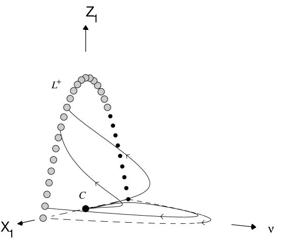
Figure 1: Phase diagram of the system (3.5)-(3.8) in the NS-NS ($\Lambda>0$) sector with $\rho\neq 0$ and $\tilde{K}=0$. The label $L^{+}$ refers to a line of equilibrium points. In this phase space, $\dot{\varphi}>0$ is assumed. The labels in all figures correspond to those equilibrium points discussed in the text. Throughout, large black dots will represent sources (i.e., repellers), large grey-filled dots will represent sinks (i.e., attractors), and small black dots will represent saddles. Grey lines represent typical trajectories found within the two-dimensional invariant sets, dashed black lines are those trajectories along the intersection of the invariant sets, and solid black lines are typical trajectories within the full three-dimensional phase space.

3.1.2 The Invariant Set $\rho=0$ for $\Lambda>0$, $\tilde{K}>0$

In the $\rho=0$ case, the system reduces to the three dimensions of $\{X_{1},Y_{1},Z_{1}\}$ ($V_{1}=1-X_{1}^{2}-Z_{1}$). The equilibrium points are the lines $L^{\pm}$ with eigenvalues $\lambda_{1}$, $\lambda_{2}$ and $\lambda_{3}$ (from Section 3.1), and the two endpoints of $L_{1}$ with eigenvalues $\lambda_{\pm}$ and $\lambda_{3}$ (from Section 3.1). These endpoints are specified by the condition $Y_{1}^{2}=1$ and we denote them by $L_{1}^{(\pm)}$, where the “$\pm$” in the superscript reflects the sign of $Y_{1}$.

For this invariant set the entire line $L^{+}$ acts as a global sink and the entire line $L^{-}$ acts as a global source. Furthermore, we note that for $L_{1}^{\pm}$, $\lambda_{-}=0$, and so these two points are non-hyperbolic. However, the eigenvectors associated with these zero eigenvalues are both $[\frac{-2}{\sqrt{3}},1,0]$ and are completely located in the $(X_{1},Y_{1})$ plane. Hence, if we choose $Z_{1}=0$ and rotate the $(X_{1},Y_{1})$ axes such that

$$\tilde{x}\equiv(Y_{1}\mp 1)-\frac{\sqrt{3}}{2}X_{1},\qquad\tilde{y}\equiv(Y_{1}\mp 1)+\frac{2}{\sqrt{3}}X_{1},$$

we see that in the vicinity of the equilibrium point, the trajectories along $\tilde{x}$ for $\tilde{y}=0$ are also along these eigenvectors. Hence, for $\tilde{y}=0$ and small $\tilde{x}$, it follows that

$$\frac{d\tilde{x}}{dT}\approx\mp\frac{\tilde{x}}{7},$$

Consequently, for $Y_{1}=+1$, the trajectory along $\tilde{x}$ asymptotes towards the equilibrium point, whereas the trajectory along $\tilde{x}$ for $Y_{1}=-1$ asymptotes away from the equilibrium point. This implies that the points $L_{1}^{\pm}$ are saddle points. The phase space is depicted in Fig. 2.

The quantity $X_{1}/\sqrt{Z_{1}}$ is monotonically decreasing. Such a monotonic function excludes the possibility of periodic or recurrent orbits in this three-dimensional space. Therefore, solutions generically asymptote into the past towards $L^{-}$ and into the future towards $L^{+}$. In this three-dimensional set, spatial curvature is dynamically important only at intermediate times.

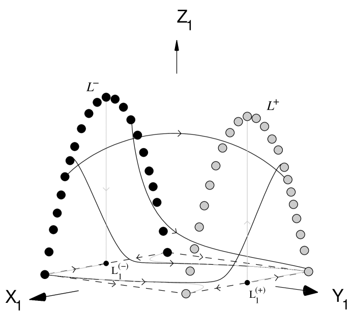
Figure 2: Phase diagram of the system (3.5)-(3.8) in the NS-NS ($\Lambda>0$) sector with $\rho=0$ and $\tilde{K}>0$. The labels $L^{+}$ and $L^{-}$ refer to lines of equilibrium points, and the labels $L_{1}^{(+)}$ and $L_{1}^{(-)}$ represent the equilibrium points which are the endpoints of the line $L_{1}$ (for which $X_{1}=+1$ and $X_{1}=-1$, respectively). In this phase space, $\dot{\varphi}>0$ is assumed. See also caption to Fig. 1.

3.1.3 Qualitative Analysis of the Four-Dimensional System

The qualitative dynamics in the full four-dimensional phase space is as follows. The past attractors are the line $L^{-}$ for $X_{1}<\frac{1}{\sqrt{3}}$ and the line $L_{1}$ for $Y_{1}>0$. The future-attractor sets are the lines $L^{+}$ for $X_{1}>\frac{-1}{\sqrt{3}}$ and the line $L_{1}$ for $Y_{1}<0$. We note that $Y_{1}/\sqrt{V_{1}}$ is monotonically increasing and this implies that there are no periodic or recurrent orbits in the full four–dimensional phase space. Therefore, solutions are generically asymptotic in the past to either the line $L^{-}$ for $h_{*}<\frac{1}{3}$ or to the line $L_{1}$ for $n>0$. Similarly, solutions are generically asymptotic in the future to either $L^{+}$ for $h_{*}>\frac{-1}{3}$ or $L_{1}$ for $n<0$.

Since $Y_{1}/\sqrt{V_{1}}$ is monotonically increasing, $Y_{1}\rightarrow+1$ or $V_{1}\rightarrow 0$ asymptotically to the future. These limits represent global sinks on the line $L^{+}$. Conversely, $Y_{1}\rightarrow-1$ or $V_{1}\rightarrow 0$ asymptotically to the past, corresponding to the global sources on the line $L^{-}$. There are also equilibrium points for finite $Y_{1}\equiv Y_{*}$ inside the phase space on the line $L_{1}$. Again, since $Y_{1}/\sqrt{V_{1}}$ is monotonically increasing, the points $Y_{*}<0$ are global sinks and $Y_{*}>0$ are global sources. All of this is consistent with the above discussion presented in Section 2.2 regarding the generic asymptotic behaviour.

We note that the reflections $X_{1}\rightarrow-X_{1}$ and $Y_{1}\rightarrow-Y_{1}$ are equivalent to a time reversal of the dynamics. Therefore, there are orbits starting on the line $L^{-}$ (for $X_{1}<\frac{1}{\sqrt{3}}$) and ending on the line $L_{1}$ (for $Y_{*}<0$). Similarly, there are orbits which begin on the line $L_{1}$ (for $Y_{*}>0$) and end on the line $L^{+}$ (for $X_{1}>\frac{-1}{\sqrt{3}}$). Due to the existence of the monotonic function and the continuity of orbits in the four-dimensional phase space, solutions cannot start and finish on $L_{1}$. This is best illustrated in the invariant set $Z_{1}=0$. In addition, orbits may start on the line $L^{-}$ (for $X_{1}<\frac{1}{\sqrt{3}}$) and end on the line $L^{+}$ (for $X_{1}>\frac{-1}{\sqrt{3}}$). Investigation of the invariant set $Z_{1}=0$ also indicates which sources and sinks are connected; not all orbits from $L^{-}$ can evolve towards $L^{+}$.

Although the lines $L^{\pm}$ lie in both of the invariant sets $\rho=0$ and $\tilde{K}=0$, the line $L_{1}$ does not. On this line, $X_{1}=0$, and the solutions are therefore static $(\dot{\alpha}=\dot{\beta}=0)$. Eq. (2.21) then implies that the axion field and spatial curvature can both be dynamically significant at early and late times for the appropriate orbits.

3.2 The Case $\Lambda>0$, $\tilde{K}<0$

In this case, we choose the negative sign for $U_{2}$ in Eq. (3.1), the positive sign for $V_{2}$, and the definition $\xi^{2}=\dot{\varphi}^{2}$. The generalized Friedmann constraint (2.16) now implies that

$$0\leq X_{2}^{2}+Z_{2}+U_{2}+V_{2}\leq 1.$$ (3.11)

For this system, $Y_{2}^{2}=1$, and so the four-dimensional system consists of the variables $0\leq\{X_{2}^{2},Z_{2},U_{2},V_{2}\}\leq 1$:

$$\frac{dX_{2}}{dT} = \sqrt{3}\left(1-X_{2}^{2}-Z_{2}-V_{2}-\frac{2}{3}U_{2}\right)+X_{2}\left(1-X_{2}^{2}-Z_{2}\right),$$ (3.12)

$$\frac{dZ_{2}}{dT} = 2Z_{2}\left(1-X_{2}^{2}-Z_{2}\right)>0,$$ (3.13)

$$\frac{dU_{2}}{dT} = -2U_{2}\left(X_{2}^{2}+Z_{2}+\frac{1}{\sqrt{3}}X_{2}\right),$$ (3.14)

$$\frac{dV_{2}}{dT} = -2V_{2}\left(X_{2}^{2}+Z_{2}\right)<0.$$ (3.15)

The invariant sets $X_{2}^{2}+Z_{2}+U_{2}+V_{2}=1$, $Z_{2}=0$, $V_{2}=0$, $U_{2}=0$ define the boundary of the phase space. The equilibrium sets and their corresponding eigenvalues (denoted by $\lambda$) are

$$S^{+}: X_{2}=-\frac{1}{\sqrt{3}},Z_{2}=0,U_{2}=\frac{2}{3},V_{2}=0;$$ (3.16)

$$\left(\lambda_{1},\lambda_{2},\lambda_{3},\lambda_{4}\right)=\left(-\frac{2}{3},\frac{2}{3},\frac{4}{3},\frac{4}{3}\right),$$

$$C: X_{2}=0,Z_{2}=0,U_{2}=0,V_{2}=1;$$ (3.17)

$$\left(\lambda_{1},\lambda_{2},\lambda_{3},\lambda_{4}\right)=\left(1,0,2,0\right),$$

$$L^{+}: Z_{2}=1-X_{2}^{2},U_{2}=0,V_{2}=0;$$ (3.18)

$$\left(\lambda_{1},\lambda_{2},\lambda_{3},\lambda_{4}\right)=\left(-\frac{2}{\sqrt{3}}\left[X_{2}+\sqrt{3}\right],-2,0,-2\sqrt{3}\left[X_{2}+\frac{1}{\sqrt{3}}\right]\right).$$

The point $C$ represents the static ‘linear dilaton–vacuum’ solution (A.4). The saddle $S^{+}$ represents the “$-$” branch of the Milne solution (A.2), where only the curvature term and scale factor are dynamic.

3.2.1 The Invariant Set $\rho=0$ for $\Lambda>0$, $\tilde{K}<0$

In the $\rho=0$ case, the system reduces to the three dimensions of $\{X_{2},Z_{2},U_{2}\}$ ($V_{2}=1-X_{2}^{2}-Z_{2}-U_{2}$). The equilibrium points are the same as above with eigenvalues $\lambda_{1}$, $\lambda_{2}$ and $\lambda_{3}$. We note that for this invariant set the entire line $L^{+}$ acts as a global sink, and $C$ acts as a source. Although one of the eigenvalues for the point $C$ is zero, it is shown in the following subsubsection that this point is a source in the full four–dimensional phase space. The argument is identical in this subsection.

The variable $Z_{2}$ is monotonically increasing, and as such we see that the shear term is negligible at early times, but becomes dynamically significant at late times. There are no periodic or recurrent orbits in this three–dimensional phase space due to the existence of this monotonic function. In general, solutions asymptote into the past towards the static solution (A.4) (point $C$). Solutions asymptote into the future towards $L^{+}$. Fig. 3 depicts this three-dimensional phase space.

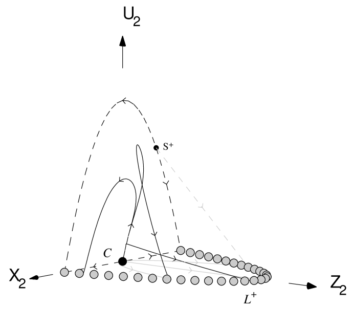
Figure 3: Phase diagram of the system (3.12)-(3.15) in the NS-NS ($\Lambda>0$) sector with $\rho=0$ and $\tilde{K}<0$. Note that $L^{+}$ represents a line of equilibrium points. See also caption to Fig. 1.

3.2.2 Qualitative Analysis of the Four-Dimensional System

The qualitative behaviour for the invariant set $\tilde{K}=0$ is discussed in Section 3.1.1 (see Fig. 1). In the four-dimensional set, the point $C$ is non-hyperbolic because of the two zero eigenvalues. However, it can be shown that this point is a source in the four-dimensional set by the following argument. We first note that the variable $Z_{2}$ is monotonically increasing and hence orbits asymptote into the past towards the invariant set $Z_{2}=0$. Similarly, $V_{2}$ is a monotonically decreasing function, and so orbits asymptote into the past towards large $V_{2}$ (i.e., $V_{2}=1$). This implies that they asymptote towards the point $C$.

Since $Z_{2}=0$ asymptotically, let us consider the invariant set $Z_{2}=0$, where Eqs. (3.12)-(3.15) become:

$$\frac{dX_{2}}{dT} = \sqrt{3}\left(1-X_{2}^{2}-V_{2}-\frac{2}{3}\tilde{U}_{2}\right)+X_{2}\left(1-X_{2}^{2}\right),$$ (3.19)

$$\frac{dU_{2}}{dT} = -2U_{2}\left(X_{2}^{2}+\frac{1}{\sqrt{3}}X_{2}\right),$$ (3.20)

$$\frac{dV_{2}}{dT} = -2V_{2}X_{2}^{2}.$$ (3.21)

It is clear from Eq. (3.21) that $V_{2}$ increases monotonically into the past. Now, this three-dimensional phase space is bounded by the surface $X_{2}^{2}+U_{2}+V_{2}=1$, the “apex” of which lies at $V_{2}=1$ (and $X_{2}=U_{2}=0$). Therefore, all orbits in or on this phase space boundary lie below $V_{2}=1$, and therefore asymptote into the past towards $V_{2}=1$. To further illustrate that this point is indeed a source, it is helpful to consider the invariant set $Z_{2}=U_{2}=0$, $X_{2}^{2}+V_{2}=1$. In the neighbourhood of $C$, Eq. (3.19) becomes $dX_{2}/dT=X_{2}(1-X_{2}^{2})$, indicating that orbits are repelled from $X_{2}=0$. Hence, the point $C$ is the past attractor to the full four-dimensional set.

The future attractor for this set is the line $L^{+}$ (for $X_{2}>\frac{-1}{\sqrt{3}}$). Both $C$ and $L^{+}$ lie in both of the invariant sets $\rho=0$ and $\tilde{K}=0$, which is consistent with the analysis of Eq. (2.21). We conclude, therefore, that the spatial curvature terms and the axion field are dynamically important only at intermediate times, and are negligible at early and late times. The dynamical effect of the shear becomes increasingly important because the variable $Z_{2}$ increases monotonically. On the other hand, the variable $V_{2}$ decreases monotonically and the dynamical effect of the central charge deficit, $\Lambda$, becomes increasingly negligible. In addition, the existence of monotone functions in the four–dimensional phase space prohibits closed orbits and serves as proof of the evolution that is described above.

3.3 The Case $\Lambda<0$, $\tilde{K}>0$

We choose the positive sign for $U_{3}$ and the negative sign for $V_{3}$ in Eq. (3.1) to ensure that these variables are positive definite. We also define $\xi^{2}\equiv\dot{\varphi}^{2}+3\tilde{K}-2\Lambda$ for this case. The generalized Friedmann constraint equation can then be rewritten as

$$0\leq X_{3}^{2}+Z_{3}\leq 1,\qquad Y_{3}^{2}+U_{3}+V_{3}=1,$$ (3.22)

We again eliminate $U_{3}$ (which is proportional to $\tilde{K}$), and consider the four-dimensional system of ODEs for $0\leq\{X_{3}^{2},Y_{3}^{2},Z_{3},V_{3}\}\leq 1$:

$$\frac{dX_{3}}{dT} = \left(1-X_{3}^{2}-Z_{3}\right)\!\!\left(\sqrt{3}+X_{3}Y_{3}\right)-\!\frac{1}{\sqrt{3}}\left(1-Y_{3}^{2}-V_{3}\right)\!\!\left(1-X_{3}^{2}-Z_{3}\right),$$ (3.23)

$$\frac{dY_{3}}{dT} = \frac{1}{\sqrt{3}}X_{3}Y_{3}\left(1-Y_{3}^{2}-V_{3}\right)+\left(1-Y_{3}^{2}\right)\left(X_{3}^{2}+Z_{3}\right),$$ (3.24)

$$\frac{dZ_{3}}{dT} = 2Z_{3}\left[\frac{1}{\sqrt{3}}X_{3}\left(1-Y_{3}^{2}-V_{3}\right)+Y_{3}\left(1-X_{3}^{2}-Z_{3}\right)\right],$$ (3.25)

$$\frac{dV_{3}}{dT} = 2V_{3}\left[\frac{1}{\sqrt{3}}X_{3}\left(1-Y_{3}^{2}-V_{3}\right)-Y_{3}\left(X_{3}^{2}+Z_{3}\right)\right].$$ (3.26)

The invariant sets $Y_{3}^{2}+V_{3}=1$, $X_{3}^{2}+Z_{3}=1$, $Z_{3}=0$ define the boundary of the phase space. The equilibrium sets and their corresponding eigenvalues (denoted by $\lambda$) are

$$L^{\pm}: Y_{3}=\pm 1,Z_{3}=1-X_{3}^{2},V_{3}=0;$$ (3.27)

$$\left(\lambda_{1},\lambda_{2},\lambda_{3},\lambda_{4}\right)=\left(\mp\frac{2}{\sqrt{3}}\left[\sqrt{3}\pm X_{3}\right],\mp 2,0,\mp 2\sqrt{3}\left[\frac{1}{\sqrt{3}}\pm X_{3}\right]\right),$$

where again the zero eigenvalues arise because these are all lines of equilibrium points. Here, the global sink is the line $L^{+}$ for $X_{3}>\frac{-1}{\sqrt{3}}$ (saddle otherwise), and the global source is the line $L^{-}$ for $X_{3}<\frac{1}{\sqrt{3}}$ (saddle otherwise). Stable solutions on the line $L^{+}$ correspond to the range $h_{*}>\frac{-1}{3}$. The stable solutions on $L^{-}$ arise when $h_{*}<\frac{1}{3}$.

3.3.1 The Invariant Set $\tilde{K}=0$ for $\Lambda<0$

This invariant set was studied in paper I, the dynamics of which are as follows. The variables $X_{3}$ and $Y_{3}$ are monotonically increasing functions, corresponding to $\dot{\alpha}$ and $\dot{\varphi}$ (respectively). The former implies that these trajectories represent cosmologies that are initially contracting and then reexpand. In paper I, the third variable used was $\kappa\equiv 1-X_{3}^{2}-Z_{3}$. This is proportional to $\rho$ and is only dynamically significant at intermediate times. It asymptoted to zero into the past and future, indicating that the axion field is negligible at early and late times. All the equilibrium points in this invariant set are represented by the dilaton-vacuum solutions (A.1) (the lines $L^{\pm}$). In general, orbits asymptote into the past towards the line $L^{-}$ (for $X_{3}<\frac{1}{\sqrt{3}}$), and asymptote to the future towards the line $L^{+}$ (for $X_{3}>\frac{-1}{\sqrt{3}}$). Fig. 4 depicts this three-dimensional phase space, using the variables $\{X_{3},Y_{3},\kappa\}$.

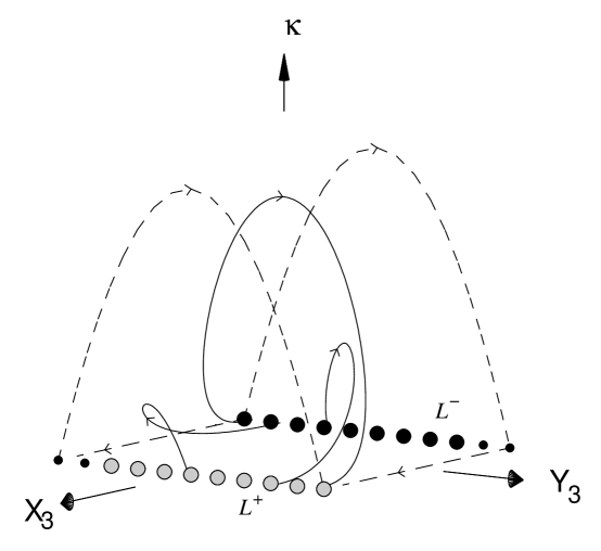
Figure 4: Phase portrait of the system (3.23)-(3.26) in the NS-NS ($\Lambda<0$) sector for $K=0$ and $\rho\neq 0$. Note that the labels $L^{+}$ and $L^{-}$ refer to lines of equilibrium points. See also caption to Fig. 1.

3.3.2 The Invariant Set $\rho=0$ for $\Lambda<0$, $\tilde{K}>0$

Since $\dot{\alpha}\neq 0$ at the equilibrium points, we examine the $\rho=0$ case, where the system reduces to the three dimensions $\{X_{3},Y_{3},V_{3}\}$ ($Z_{3}=1-X_{3}^{2}$). The equilibrium points are the same as above with eigenvalues $\lambda_{1}$, $\lambda_{2}$, $\lambda_{3}$. We note that the entire line $L^{+}$ acts as a global sink and that the entire line $L^{-}$ acts as a global source in this invariant set. The function $Y_{3}/\sqrt{V_{3}}$ is monotonically increasing, eliminating the possibility of periodic orbits. Fig. 5 depicts this three-dimensional phase space.

Figure 5: Phase diagram of the system (3.23)-(3.26) in the NS-NS ($\Lambda<0$) sector for $\rho=0$ and $\tilde{K}>0$. Note that $L^{+}$ and $L^{-}$ represent lines of equilibrium points. See also caption to Fig. 1.

3.3.3 Qualitative Analysis of the Four-Dimensional System

The qualitative dynamics in the full four-dimensional phase space is as follows. The global repellers and attractors are the lines $L^{-}$ and $L^{+}$, respectively. Orbits generically asymptote into the past towards the line $L^{-}$ (for $X_{3}<\frac{1}{\sqrt{3}}$), and into the future towards $L^{+}$ (for $X_{3}>\frac{-1}{\sqrt{3}}$). In the former case the stable solutions are given by the “$+$’ branch of Eq. (A.1) for $h_{*}<\frac{1}{3}$. The stable sinks are given by the “$-$” branch with $h_{*}>\frac{-1}{3}$. Again, we see that the curvature term, axion field and the central charge deficit are dynamically important only at intermediate times. The existence of the monotonically increasing function $Y_{3}/\sqrt{V_{3}}$ excludes the possibility of periodic orbits and serves to verify the above description of the evolution of the solutions in the four–dimensional set.

3.4 The Case $\Lambda<0$, $\tilde{K}<0$

For this case, the appropriate definition for the variable $\xi$ is $\xi^{2}=\dot{\varphi}^{2}-2\Lambda$ and we choose the negative signs for both $U_{4}$ and $V_{4}$ in Eq. (3.1). The generalized Friedmann constraint equation is written as

$$0\leq X_{4}^{2}+Z_{4}+U_{4}\leq 1,\qquad Y_{4}^{2}+V_{4}=1,$$ (3.28)

Treating $V_{4}$ as the extraneous variable results in the four-dimensional system consisting of the variables $0\leq\{X_{4}^{2},Y_{4}^{2},Z_{4},U_{4}\}\leq 1$:

$$\frac{dX_{4}}{dT} = \left(1-X_{4}^{2}-Z_{4}\right)\left(\sqrt{3}+X_{4}Y_{4}\right)-\frac{2}{\sqrt{3}}U_{4},$$ (3.29)

$$\frac{dY_{4}}{dT} = \left(1-Y_{4}^{2}\right)\left(X_{4}^{2}+Z_{4}\right)>0,$$ (3.30)

$$\frac{dZ_{4}}{dT} = 2Z_{4}Y_{4}\left(1-X_{4}^{2}-Z_{4}\right),$$ (3.31)

$$\frac{dU_{4}}{dT} = -2U_{4}\left[Y_{4}\left(X_{4}^{2}+Z_{4}\right)+\frac{1}{\sqrt{3}}X_{4}\right].$$ (3.32)

The invariant sets $X_{4}^{2}+Z_{4}+U_{4}=1$, $Z_{4}=0$, $Y_{4}^{2}=1$, $U_{4}=0$ define the boundary of the phase space. The equilibrium sets and their corresponding eigenvalues (denoted by $\lambda$) are

$$S^{\pm}: X_{4}=\mp\frac{1}{\sqrt{3}},Y_{4}=\pm 1,Z_{4}=0,U_{4}=\frac{2}{3};$$ (3.33)

$$\left(\lambda_{1},\lambda_{2},\lambda_{3},\lambda_{4}\right)=\left(\pm\frac{2}{3},\mp\frac{2}{3},\pm\frac{4}{3},\pm\frac{4}{3}\right),$$

$$L^{\pm}: Y_{4}=\pm 1,Z_{4}=1-X_{4}^{2},U_{4}=0;$$ (3.34)

$$\left(\lambda_{1},\lambda_{2},\lambda_{3},\lambda_{4}\right)=\left(\mp\frac{2}{\sqrt{3}}\left[\sqrt{3}\pm X_{4}\right],\mp 2,0,\mp 2\sqrt{3}\left[\frac{1}{\sqrt{3}}\pm X_{4}\right]\right).$$

The global source for this system is the line $L^{-}$ (for $X_{4}<\frac{1}{\sqrt{3}}$, $h_{*}<\frac{1}{3}$) and the global sink is the line $L^{+}$ (for $X_{4}>\frac{-1}{\sqrt{3}}$, $h_{*}>\frac{-1}{3}$). The saddle points, $S^{\pm}$, are represented by the Milne models (A.2), where $S^{+}$ corresponds to the “$-$” solution and $S^{-}$ to the “$+$” solution.

3.4.1 The Invariant Set $\rho=0$ for $\Lambda<0$, $\tilde{K}<0$

This system reduces to the three dimensions of $\{X_{4},Y_{4},Z_{4}\}$ ($U_{4}=1-X_{4}^{2}-Z_{4}$). The equilibrium points are the same as above with eigenvalues $\lambda_{1}$, $\lambda_{2}$, $\lambda_{3}$. The entire lines $L^{+}$ and $L^{-}$ now act as a global sink and source, respectively. Recurrent orbits are forbidden by the existence of the monotonically increasing variable $Y_{4}$. Hence, solutions generically asymptote into the past (future) towards the “$+$” (“$-$”) dilaton–vacuum solutions (A.1) and the curvature term and central charge deficit are dynamically significant only at intermediate times. Fig. 6 depicts this three-dimensional phase space.

Figure 6: Phase portrait of the system (3.29)-(3.32) in the NS-NS ($\Lambda<0$) sector with $\rho=0$ and $\tilde{K}<0$. Note that $L^{+}$ and $L^{-}$ represent lines of equilibrium points. See also caption to Fig. 1.

3.4.2 Qualitative Analysis of the Four-Dimensional System

The dynamical behaviour in the invariant set $\tilde{K}=0$ is identical to that described in Section 3.3.1 (see Fig. 4). The qualitative dynamics in the full four-dimensional phase space is as follows. Since $Y_{4}$ is monotonically increasing, the orbits asymptote into the past towards $Y_{4}=-1$ and into the future towards $Y_{4}=+1$. As in the above examples, the existence of such a monotonic function excludes the possibility of periodic orbits in the four–dimensional phase space. Most orbits asymptote into the past towards the line $L^{-}$ (for $X_{4}<\frac{1}{\sqrt{3}}$), and into the future towards the line $L^{+}$ (for $X_{4}>\frac{-1}{\sqrt{3}}$). The range of values for $h_{*}$ corresponding to stable solutions is given by $h_{*}>\frac{-1}{3}$ for those on $L^{+}$ and $h_{*}<\frac{1}{3}$ for those on $L^{-}$. The variable $Y_{4}$ increases monotonically along orbits and this implies that $\dot{\varphi}$ is dynamically significant at early and late times, but dynamically insignificant at intermediate times. Conversely, we see that the curvature term, central charge deficit and axion field are dynamically important only at intermediate times, and are negligible at early and late times.

This concludes the qualitative analysis of the isotropic curvature string cosmologies with NS–NS fields. In the next Section, we consider the effect on the dynamics of introducing a non–trivial $\Lambda_{\rm M}$.

4 Non-Zero Cosmological Constant $\Lambda_{\rm M}$ ($\Lambda=0$)

We begin this Section by defining new variables

$$\frac{d}{dt}\equiv e^{\frac{1}{2}(\varphi+3\alpha)}\frac{d}{dT},\quad N\equiv 6{\beta^{\prime}}^{2},\qquad\psi\equiv\varphi^{\prime},\qquad h\equiv\alpha^{\prime},\qquad K\equiv\tilde{K}e^{-(\varphi+3\alpha)},$$ (4.1)

where a prime denotes differentiation with respect to the new time coordinate, $T$. Eqs. (2.11)–(2.16) may then be written as the set of ODEs:

$$h^{\prime} = -\frac{3}{2}h^{2}+\frac{1}{2}h\psi-K-\frac{1}{2}\Lambda_{\rm M}+\frac{1}{2}\rho e^{-(\varphi+3\alpha)}$$ (4.2)

$$\psi^{\prime} = \frac{3}{2}h^{2}-\frac{3}{2}h\psi+\frac{1}{2}N+\frac{3}{2}K-\frac{1}{4}\rho e^{-(\varphi+3\alpha)}$$ (4.3)

$$N^{\prime} = (\psi-3h)N$$ (4.4)

$$K^{\prime} = -(\psi+5h)K$$ (4.5)

$$\rho^{\prime} = -6h\rho$$ (4.6)

$$3h^{2} - \psi^{2}+N-3K+\Lambda_{\rm M}+\frac{1}{2}\rho e^{-(\varphi+3\alpha)}=0$$ (4.7)

The variable $\rho$ may be eliminated due to the constraint equation (2.16). It also proves convenient to further define a set of variables

$$\mu\equiv\frac{\sqrt{3}h}{\xi},\quad\chi\equiv\frac{\psi}{\xi},\quad\nu\equiv\frac{N}{\xi^{2}},\quad\zeta\equiv\frac{\pm 3K}{\xi^{2}},\quad\lambda\equiv\frac{\pm\Lambda_{\rm M}}{\xi^{2}},\quad\frac{d}{dT}\equiv\xi\frac{d}{d\tau},$$ (4.8)

where the $\pm$ signs ensure that $\zeta>0$ and $\lambda>0$. The variable $\xi$ is defined in each of the following four subsections by

• $\Lambda_{\rm M}>0$

  • $K>0$: $\xi^{2}\equiv 3K+\psi^{2}$ (Section 4.1),

  • $K<0$: $\xi^{2}\equiv\psi^{2}$ (Section 4.2),

• $\Lambda_{\rm M}<0$

  • $K>0$: $\xi^{2}\equiv 3K+\psi^{2}-\Lambda_{\rm M}$ (Section 4.3),

  • $K<0$: $\xi^{2}\equiv\psi^{2}-\Lambda_{\rm M}$ (Section 4.4).

With these definitions, all variables are bounded, $0\leq\{\mu^{2},\chi^{2},\nu,\zeta,\lambda\}\leq 1$, and Eq. (4.7) now reads

$$\frac{1}{2}\rho\xi^{-2}e^{-(\varphi+3\alpha)}=\chi^{2}\pm\zeta\mp\lambda-\mu^{2}-\nu>0.$$ (4.9)

Our overall approach in this Section is identical to that of Section 3 and we refer the reader to the discussion immediately after Eq. (3.2) for the general outline adopted.

4.1 The Case $\Lambda_{\rm M}>0$, $K>0$

For $K>0$, Eq. (4.7) is written in the new variables as

$$0\leq\mu_{1}^{2}+\nu_{1}+\lambda_{1}\leq 1,\qquad\zeta_{1}+\chi_{1}^{2}=1,$$ (4.10)

where the “$+$” sign is chosen for both $\lambda$ and $\zeta$ in Eq. (4.8). For this case, the variable $\zeta_{1}\equiv 1-\chi_{1}^{2}$ will be considered extraneous and the system (4.2)-(4.5) then reduces to the four-dimensional system:

$$\frac{d\mu_{1}}{d\tau} = \left(1-\!\mu_{1}^{2}-\!\nu_{1}-\!\frac{1}{2}\lambda_{1}\right)\!\left(\sqrt{3}+\!\mu_{1}\chi_{1}\right)-\frac{1}{\sqrt{3}}\left(1-\!\mu_{1}^{2}\right)\!\left(1-\!\chi_{1}^{2}\right)-\sqrt{3}\lambda_{1},$$ (4.11)

$$\frac{d\chi_{1}}{d\tau} = \left(1-\chi_{1}^{2}\right)\left[\mu_{1}^{2}+\nu_{1}+\frac{1}{2}\lambda_{1}+\frac{1}{\sqrt{3}}\mu_{1}\chi_{1}\right],$$ (4.12)

$$\frac{d\nu_{1}}{d\tau} = \nu_{1}\left[\frac{2}{\sqrt{3}}\mu_{1}\left(1-\chi_{1}^{2}\right)+2\chi_{1}\left(1-\mu_{1}^{2}-\nu_{1}-\frac{1}{2}\lambda_{1}\right)\right],$$ (4.13)

$$\frac{d\lambda_{1}}{d\tau} = \lambda_{1}\left[\frac{1}{\sqrt{3}}\mu_{1}\left(5-2\chi_{1}^{2}\right)+\chi_{1}\left(1-2\mu_{1}^{2}-2\nu_{1}-\lambda_{1}\right)\right].$$ (4.14)

The invariant sets $\mu_{1}^{2}+\nu_{1}+\lambda_{1}=1$ ($\rho=0$), $\chi_{1}^{2}=1$ ($K=0$), $\nu_{1}=0$ ($N=0$) and $\lambda_{1}=0$ ($\Lambda_{\rm M}=0$) define the boundaries to the phase space. The equilibrium points and their respective eigenvalues (denoted by $\lambda$) are given by

$$L^{\pm}: \chi_{1}=\pm 1,\mu_{1}^{2}+\nu_{1}=1,\lambda_{1}=0;$$

$$(\lambda_{1},\lambda_{2},\lambda_{3},\lambda_{4})=\left(0,\mp\frac{2}{\sqrt{3}}\left[\sqrt{3}\pm\mu_{1}\right],\sqrt{3}\left[\mu_{1}\mp\frac{1}{\sqrt{3}}\right],\mp 2\sqrt{3}\left[\frac{1}{\sqrt{3}}\pm\mu\right]\right).$$

$$S^{\pm}_{1}: \mu_{1}=\mp\frac{1}{\sqrt{27}},\chi_{1}=\pm 1,\nu_{1}=0,\lambda_{1}=\frac{16}{27};$$ (4.16)

$$\left(\lambda_{1},\lambda_{2},\lambda_{3},\lambda_{4}\right)=\left(\mp\frac{1}{3}\left[1+i\frac{\sqrt{231}}{3}\right],\mp\frac{1}{3}\left[1-i\frac{\sqrt{231}}{3}\right],\mp\frac{4}{3},\pm\frac{4}{9}\right).$$

From the eigenvalues, we deduce that $L^{+}$ is a late-time attractor for $\mu_{1}^{2}<\frac{1}{3}$, and that $L^{-}$ is an early-time repeller for $\mu_{1}^{2}<\frac{1}{3}$. In both cases, $\chi_{1}^{2}=1$ and therefore $K=0$ ($\zeta_{1}=0$). The “$+$” solution of (A.1) is a sink for $h_{*}^{2}<\frac{1}{9}$ and the “$-$” solution of (A.1) is a source for $h_{*}<\frac{1}{9}$. The points $S^{\pm}_{1}$ are saddle points on the boundary of the phase space and correspond to the exact solution (A.5).

4.1.1 The Invariant Set $K=0$ for $\Lambda_{\rm M}>0$

This invariant set was studied in paper II by employing dynamical variables equivalent to $\{\mu_{1},\lambda_{1},\nu_{1}\}$, and we now summarize the important features of the model. For spatially isotropic solutions confined to the invariant set $\nu_{1}=0$, most trajectories evolve from the equilibrium point $S^{+}_{1}$ (labelled “$F$” in paper II) located at $(\mu_{1},\nu_{1},\lambda_{1})=(\frac{-1}{\sqrt{27}},0,\frac{16}{27})$ (corresponding to the “$-$” solution (A.5)) and are future asymptotic to a heteroclinic orbit. There are two saddle equilibrium points, $S_{1}$ and $S_{2}$, which are the endpoints of the line $L^{+}$; $S_{1}$ is given by the “$-$” branch of Eq. (A.1) with $h_{*}=\frac{-1}{\sqrt{3}}$ and $S_{2}$ corresponds to $h_{*}=\frac{1}{\sqrt{3}}$. There are also the single boundary orbits in the invariant sets $\lambda_{1}=0$, corresponding to $\Lambda_{\rm M}=0$ and $\lambda_{1}+\mu_{1}^{2}=1$ (constant axion field). An orbit spends the majority of its time in the neighbourhoods of $S_{1}$ and $S_{2}$ and shadows the respective boundary orbits as it rapidly moves between the two saddles. Progressively more time is spent near the saddles for each completed cycle, and the dynamics is therefore not periodic.

An anisotropic contribution $(\nu_{1}\neq 0)$ does not introduce new sources into the system and the point $S_{1}^{+}$ is still the only source. Fig. 7 depicts the full three-dimensional space. Eq. (4.13) implies that $\nu_{1}$ is a monotonically increasing function and consequently the orbits are repelled from $S_{1}^{+}$ and spiral out monotonically. The general behaviour for most trajectories in this phase space is to evolve away from the equilibrium point $S_{1}^{+}$, spiral about the line $\mu_{1}=\frac{-1}{\sqrt{27}}$, $\nu_{1}=\frac{13}{8}(\lambda_{1}-\frac{16}{27})$ and eventually asymptote towards the line $L^{+}$ for $\mu_{1}^{2}<\frac{1}{3}$. These trajectories were discussed in detail in paper II.

Figure 7: Phase portrait of the system (4.11)-(4.13) for $\Lambda_{\rm M}>0$ with $\rho\neq 0$ and $K=0$. Note that the label $L^{+}$ refers to a line of equilibrium points. In this phase space, $\dot{\varphi}>0$ is assumed. See also caption to Fig. 1.

4.1.2 The Invariant Set $\rho=0$ for $\Lambda_{\rm M}>0$, $K>0$

For the invariant set $\rho=0$, the system (4.11)-(4.14) reduces to the three dimensions $\{\mu_{1},\chi_{1},\nu_{1}\}$ ($\lambda_{1}=1-\mu_{1}^{2}-\nu_{1}$). In this invariant set, $\mu$ is a monotonically decreasing function, and so the possibility of periodic orbits is excluded. The only equilibrium points are the lines $L^{\pm}$ with the first three eigenvalues in Eq. (LABEL:Lpm), and therefore the early and late time attractors are the lines $L^{-}$ (for $\mu_{1}>\frac{-1}{\sqrt{3}}$, $h_{*}>\frac{-1}{3}$) and $L^{+}$ (for $\mu_{1}<\frac{1}{\sqrt{3}}$, $h_{*}<\frac{1}{3}$). The curvature and cosmological constant are only dynamically significant at intermediate times and the phase space is depicted in Fig. 8.

Figure 8: Phase portrait of the system (4.11)-(4.13) for $\Lambda_{\rm M}>0$ with $\rho=0$ field and $K>0$. Note that $L^{+}$ and $L^{-}$ represent lines of equilibrium points. See also caption to Fig. 1.

4.1.3 Qualitative Analysis of the Four-Dimensional System

The qualitative dynamics in the full four-dimensional phase space is as follows. The function $\chi_{1}\nu_{1}^{\frac{1}{2}}\left(1-\mu_{1}^{2}-\nu_{1}-\lambda_{1}\right)^{\frac{1}{6}}\lambda_{1}^{-\frac{1}{3}}$ monotonically increases and so there can be no periodic orbits. The only past–attractors belong to the line $L^{-}$ for $\mu_{1}^{2}<\frac{1}{3}$ $(h_{*}^{2}<\frac{1}{9})$ and the only future attractors belong to the line $L^{+}$ for $\mu_{1}^{2}<\frac{1}{3}$ $(h_{*}^{2}<\frac{1}{9})$. Both lines $L^{\pm}$ lie in both of the invariant sets $\rho=0$ and $\tilde{K}=0$, which is consistent with the analysis of Eq. (2.21). This implies that the spatial curvature, cosmological constant and axion field are only dynamically significant at intermediate times.

For orbits in the four-dimensional phase space, the complex eigenvalues of the saddle point $S^{\pm}_{1}$ suggest that the heteroclinic sequences may exist in the four–dimensional set. Indeed, those orbits which asymptote to the $\tilde{K}=0$ invariant set do generically end in a heteroclinic sequence, interpolated between two equilibrium points representing two dilaton–vacuum solutions, as discussed in Section 4.1.1. However, for those orbits which asymptote towards the $\rho=0$ invariant set, there are no heteroclinic sequences (as is evident from Fig. 8).

4.2 The Case $\Lambda_{\rm M}>0$, $K<0$

For $K<0$, Eq. (4.7) is written in the new variables as

$$0\leq\mu_{2}^{2}+\nu_{2}+\zeta_{2}+\lambda_{2}\leq 1,\qquad\chi_{2}^{2}=1,$$ (4.17)

where the “$+$” sign for $\lambda$ and the “$-$” sign for $\zeta$ have been chosen in Eq. (4.8). For this case, we explicitly choose $\chi_{2}=+1$, as $\chi_{2}=-1$ corresponds to a time reversal of Eqs. (4.2)–(4.6). The system (4.2)-(4.5) then reduces to the four-dimensional system:

$$\frac{d\mu_{2}}{d\tau} = \left(1-\mu_{2}^{2}-\nu_{2}-\frac{1}{2}\lambda_{2}\right)\left(\sqrt{3}+\mu_{2}\right)-\sqrt{3}\left(\lambda_{2}+\frac{2}{3}\zeta_{2}\right),$$ (4.18)

$$\frac{d\nu_{2}}{d\tau} = 2\nu_{2}\left(1-\mu_{2}^{2}-\nu_{2}-\frac{1}{2}\lambda_{2}\right),$$ (4.19)

$$\frac{d\zeta_{2}}{d\tau} = -2\zeta_{2}\left(\mu_{2}^{2}+\nu_{2}+\frac{1}{2}\lambda_{2}+\frac{1}{\sqrt{3}}\mu_{2}\right),$$ (4.20)

$$\frac{d\lambda_{2}}{d\tau} = \lambda_{2}\left(1-2\mu_{2}^{2}-2\nu_{2}-\lambda_{2}+\sqrt{3}\mu_{2}\right).$$ (4.21)

The invariant sets $\mu_{2}^{2}+\nu_{2}+\zeta_{2}+\lambda_{2}=1$ ($\rho=0$), $\zeta_{2}=0$ ($K=0$), $\nu_{1}=0$ ($N=0$) and $\lambda_{1}=0$ ($\Lambda_{\rm M}=0$) define the boundaries to the phase space. The equilibrium points and their respective eigenvalues (denoted by $\lambda$) are given by

$$S^{+}: \mu_{2}=-\frac{1}{\sqrt{3}},\zeta_{2}=\frac{2}{3},\lambda_{2}=0,\nu_{2}=0;$$ (4.22)

$$(\lambda_{1},\lambda_{2},\lambda_{3},\lambda_{4})=\frac{1}{3}(2,4,-2,4)$$

$$N: \mu_{2}=-\frac{\sqrt{3}}{5},\nu_{2}=0,\zeta_{2}=\frac{18}{25},\lambda_{2}=\frac{4}{25};$$ (4.23)

$$(\lambda_{1},\lambda_{2},\lambda_{3},\lambda_{4})=\frac{2}{5}(1+i\sqrt{2},1-i\sqrt{2},4,2)$$

$$L^{+}: \mu_{2}^{2}+\nu_{2}=1,\zeta_{2}=0,\lambda_{2}=0;$$

$$(\lambda_{1},\lambda_{2},\lambda_{3},\lambda_{4})=\left(0,-\frac{2}{\sqrt{3}}\left[\mu_{2}+\sqrt{3}\right],\sqrt{3}\left[\mu_{2}-\frac{1}{\sqrt{3}}\right],-2\sqrt{3}\left[\mu_{2}+\frac{1}{\sqrt{3}}\right]\right).$$

From the eigenvalues, it is clear that $L^{+}$ is a late-time attractor for $\mu_{2}^{2}<\frac{1}{3}$ ($h_{*}^{2}<\frac{1}{9}$). The point $N$ inside the phase space is the early-time attractor for the system, and represents the curvature–driven solution (A.6). The saddle point $S^{+}$ corresponds to the “$-$” branch of the Milne solution (A.2).

4.2.1 The Invariant Set $\rho=0$ for $\Lambda_{\rm M}>0$, $K<0$

For this invariant set, the four-dimensional system (4.18)-(4.21) reduces to a three-dimensional system involving the coordinates $\{\mu_{2},\nu_{2},\lambda_{2}\}$ ($\zeta_{2}=1-\mu_{2}^{2}-\nu_{2}-\lambda_{2}$). The equilibrium points are the same as for the full four-dimensional set, but the eigenvalues are now ($\lambda_{1},\lambda_{2},\lambda_{3}$). The variable $\nu$ is a monotonically increasing function, the existence of which eliminates the possibility of recurrent orbits. Thus, the generic behaviour of this model is for solutions to asymptote into the past towards the curvature–dominated solution (A.6), represented by the point $N$, and to the future towards the line $L^{+}$ for $\mu_{2}<\frac{1}{\sqrt{3}}$ ($h_{*}<\frac{1}{3}$). Fig. 9 depicts this phase space.

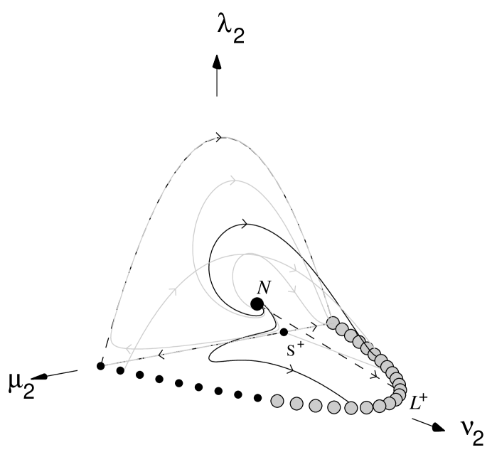
Figure 9: Phase portrait of the system (4.18)-(4.19) for $\Lambda_{\rm M}>0$ with $\rho=0$ and $K<0$. Note that $L^{+}$ represents a line of equilibrium points. In this phase space, $\dot{\varphi}>0$ is assumed. See also caption to Fig. 1.

4.2.2 Qualitative Analysis of the Four-Dimensional System

The invariant set $K=0$ was described in Section 4.1.1 (see Fig. 7). In the full four-dimensional set, the point $N$ is the early-time attractor, and $L^{+}$ is the late-time attractor for $\mu_{2}^{2}<\frac{1}{3}$ ($h_{*}^{2}<\frac{1}{9}$). The point $N$ lies in the invariant set $\rho=0$ and $L^{+}$ lies in both of the invariant sets $\rho=0$ and $\tilde{K}=0$. This is consistent with the analysis of Eq. (2.21). We see that $\nu_{2}$ is a monotonically increasing function, and so there are no recurrent or periodic orbits. Furthermore, since $\nu_{2}$ increases monotonically, the shear in the model is initially dynamically trivial, but becomes significant asymptotically into the future. The axion field and cosmological constant are only dynamically important at intermediate times and do not play a rôle in the early- and late-time behaviour of the cosmologies. The curvature term is dynamically significant at early and intermediate times, but becomes dynamically trivial at late times.

Orbits which asymptote into the future towards the $K=0$ invariant set generically end in a heteroclinic sequence, as described in Section 4.1.1 and depicted in Fig. 7. However, such a sequence does not occur for orbits which asymptote into the future towards the $\rho=0$ invariant set. Indeed, by examining the eigenvalues of the equilibrium points of the four-dimensional system, there do not seem to be heteroclinic sequences outside of the $\tilde{K}=0$ invariant set.

4.3 The Case $\Lambda_{\rm M}<0$, $K>0$

For completeness we now consider the cases where $\Lambda_{\rm M}<0$. When $K>0$, Eq. (4.7) is written in terms of the new variables as

$$0\leq\mu_{3}^{2}+\nu_{3}\leq 1,\qquad\chi_{3}^{2}+\zeta_{3}+\lambda_{3}=1,$$ (4.25)

where the “$-$” sign for $\lambda$ and the “$+$” sign for $\zeta$ have been chosen in Eq. (4.8). The variable $\lambda_{3}$ is chosen as the extraneous variable and the system (4.2)-(4.5) then reduces to the four-dimensional system:

$$\frac{d\mu_{3}}{d\tau} = \left(1-\mu_{3}^{2}-\nu_{3}\right)\left(\sqrt{3}+\mu_{3}\chi_{3}\right)+\frac{\sqrt{3}}{2}\left(1-\mu_{3}^{2}\right)\left(1-\chi_{3}^{2}-\frac{5}{3}\zeta_{3}\right),$$ (4.26)

$$\frac{d\chi_{3}}{d\tau} = -\frac{\sqrt{3}}{2}\left[\mu_{3}\chi_{3}\left(1-\chi_{3}^{2}-\frac{5}{3}\zeta_{3}\right)\right]-\frac{1}{2}\left(1-\chi_{3}^{2}\right)\left(1-2\mu_{3}^{2}-2\nu_{3}\right)+\frac{1}{2}\zeta_{3}$$

$$\frac{d\nu_{3}}{d\tau} = \nu_{3}\left[2\chi_{3}\left(1-\mu_{3}^{2}-\nu_{3}\right)-\sqrt{3}\mu_{3}\left(1-\chi_{3}^{2}-\frac{5}{3}\zeta_{3}\right)\right],$$ (4.28)

$$\frac{d\zeta_{3}}{d\tau} = -\zeta_{3}\left[2\chi_{3}\left(\mu_{3}^{2}+\nu_{3}\right)+\frac{1}{\sqrt{3}}\mu_{3}\left(5-3\chi_{3}^{2}-5\zeta_{3}\right)\right].$$ (4.29)

The invariant sets $\mu_{3}^{2}+\nu_{3}=1$, $\chi_{3}^{2}+\zeta_{3}=1$, $\nu_{3}=0$ and $\zeta_{3}=0$ define the boundary to the phase space. The equilibrium sets and their corresponding eigenvalues (denoted by $\lambda$) are

$$L^{\pm}: \chi_{3}=\pm 1,\mu_{3}^{2}+\nu_{3}=1,\zeta_{3}=0;$$

$$(\lambda_{1},\lambda_{2},\lambda_{3},\lambda_{4})=\left(0,\mp\frac{2}{\sqrt{3}}\left[\sqrt{3}\pm\mu_{3}\right],\sqrt{3}\left[\mu_{3}\mp\frac{1}{\sqrt{3}}\right],-2\sqrt{3}\left[\mu_{3}\pm\frac{1}{\sqrt{3}}\right]\right),$$

$$R: \chi_{3}=-\frac{1}{\sqrt{3}},\mu_{3}=-1,\nu_{3}=0,\zeta_{3}=0;$$ (4.31)

$$(\lambda_{1},\lambda_{2},\lambda_{3},\lambda_{4})=\frac{1}{\sqrt{3}}\left(1,2,6,10\right),$$

$$A: \chi_{3}=\frac{1}{\sqrt{3}},\mu_{3}=1,\nu_{3}=0,\zeta_{3}=0;$$ (4.32)

$$(\lambda_{1},\lambda_{2},\lambda_{3},\lambda_{4})=-\frac{1}{\sqrt{3}}\left(1,2,6,10\right).$$

Here, there are two early-time attractors. The first is the point $R$, representing the “$+$” branch of the constant axion, spatially isotropic solution (A.7), where $\dot{\varphi}<0$. The second is the line $L^{-}$ for $\mu_{3}^{2}<\frac{1}{3}$ ($h_{*}^{2}<\frac{1}{9}$). Likewise, there are two late-time attractors: these are the point $A$, representing the “$-$” solution of Eq. (A.7), where $\dot{\varphi}>0$, and the line $L^{+}$ for $\mu_{3}^{2}<\frac{1}{3}$ ($h_{*}^{2}<\frac{1}{9}$).

4.3.1 The Invariant Set $K=0$ for $\Lambda_{\rm M}<0$

In paper II, this invariant set was examined using variables which are the same as $\{\mu_{3},\chi_{3},\nu_{3}\}$. There it was shown that $\mu_{3}$ is monotonically increasing, so that most trajectories in this phase space represent bouncing cosmologies which are initially contracting. Most trajectories asymptote into the past towards either $L^{-}$ or to $R$ (see above). To the future, most orbits asymptote towards either $L^{+}$ or $A$. Fig. 10 depicts this three-dimensional phase space.

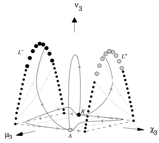
Figure 10: Phase portrait of the system (4.26)-(4.29) for $\Lambda_{\rm M}<0$ with $\rho\neq 0$ and $K=0$. Note that the labels $L^{+}$ and $L^{-}$ refer to lines of equilibrium points. See also caption to Fig. 1.

4.3.2 The Invariant Set $\rho=0$ for $\Lambda_{\rm M}<0$, $K>0$

For this invariant set, the four-dimensional system (4.26)-(4.29) reduces to a three-dimensional system involving the coordinates $\{\mu_{3},\chi_{3},\zeta_{3}\}$ ($\nu_{3}=1-\mu_{2}^{3}$). The equilibrium points are the same as the full four-dimensional set, but with eigenvalues ($\lambda_{1},\lambda_{2},\lambda_{3}$), and so the line $L^{-}$ is a source for $\mu_{3}>\frac{-1}{\sqrt{3}}$ ($h_{*}>\frac{-1}{3}$) and the line $L^{+}$ is a sink for $\mu_{3}<\frac{1}{\sqrt{3}}$ ($h_{*}<\frac{1}{3}$). The function $\chi_{3}/\sqrt{\nu_{3}}$ is monotonically increasing, and so there are no recurring or periodic orbits. Hence, solutions generically asymptote into the past towards $L^{-}$ or $R$ and into the future towards $L^{+}$ or $A$.

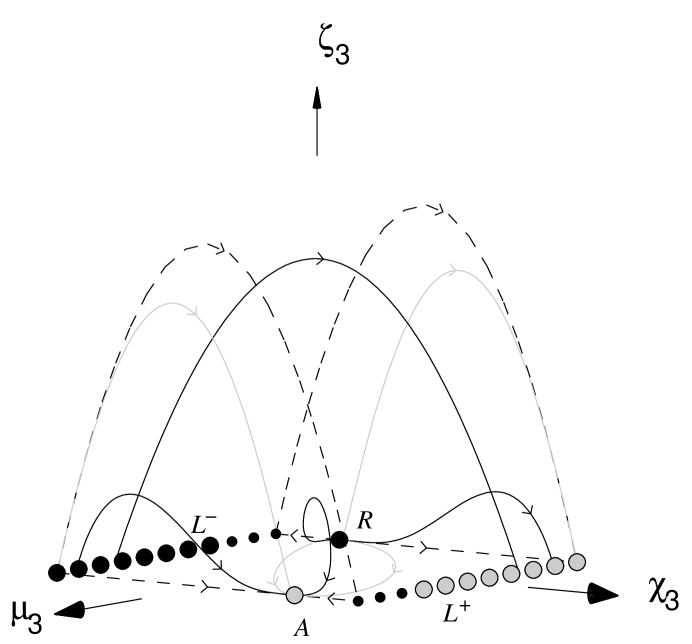
Figure 11: Phase portrait of the system (4.26)-(4.29) for $\Lambda_{\rm M}<0$ with $\rho=0$ and $K>0$. Note that $L^{+}$ and $L^{-}$ represent lines of equilibrium points. See also caption to Fig. 1.

4.3.3 Qualitative Analysis of the Four-Dimensional System

The function $\left(\chi_{3}+\frac{1}{\sqrt{3}}\mu_{3}\right)/\sqrt{\nu_{3}}$ is monotonically increasing, and so there are no recurring or periodic orbits in the full four-dimensional set. The early-time attractors are the line $L^{-}$ for $\mu_{3}^{2}<\frac{1}{3}$ ($h_{*}^{2}<\frac{1}{9}$) and the point $R$. The late-time attractors are the line $L^{+}$ for $\mu_{3}^{2}<\frac{1}{3}$ ($h_{*}^{2}<\frac{1}{9}$) and the point $A$. All of these attractors lie in both of the invariant sets $\rho=0$ and $\tilde{K}=0$ and the axion field and curvature term are dynamically significant only at intermediate times. For early and late times, the cosmological constant is dynamically important only when the shear is dynamically trivial (e.g., the points $R$ and $A$), and vice-versa (e.g., the lines $L^{\pm}$).

4.4 The Case $\Lambda_{\rm M}<0$, $K<0$

For this case, Eq. (4.7) is written in terms of the new variables as

$$0\leq\mu_{4}^{2}+\nu_{4}+\zeta_{4}\leq 1,\qquad\chi_{4}^{2}+\lambda_{4}=1,$$ (4.33)

where the “$-$” sign for both $\lambda$ and $\zeta$ has been chosen in Eq. (4.8). The variable $\lambda_{4}$ is chosen as the extraneous variable and the system (4.2)-(4.5) then reduces to the four-dimensional system:

$$\frac{d\mu_{4}}{d\tau} = \left(1-\mu_{4}^{2}-\nu_{4}\right)\left(\sqrt{3}+\mu_{4}\chi_{4}\right)+\frac{\sqrt{3}}{2}\left(1-\mu_{4}^{2}\right)\left(1-\chi_{4}^{2}\right)-\frac{2}{\sqrt{3}}\zeta_{4},$$ (4.34)

$$\frac{d\chi_{4}}{d\tau} = -\frac{1}{2}\left(1-\chi_{4}^{2}\right)\left[1-2\mu_{4}^{2}-2\nu_{4}+\sqrt{3}\mu_{4}\chi_{4}\right],$$ (4.35)

$$\frac{d\nu_{4}}{d\tau} = \nu_{4}\left[2\chi_{4}\left(1-\mu_{4}^{2}-\nu_{4}\right)-\sqrt{3}\mu_{4}\left(1-\chi_{4}^{2}\right)\right],$$ (4.36)

$$\frac{d\zeta_{4}}{d\tau} = -\zeta_{4}\left[2\chi_{4}\left(\mu_{4}^{2}+\nu_{4}\right)+\frac{1}{\sqrt{3}}\mu_{4}\left(5-3\chi_{4}^{2}\right)\right].$$ (4.37)

The invariant sets $\mu_{4}^{2}+\nu_{4}+\zeta_{4}=1$, $\chi_{4}^{2}=1$, $\nu_{4}=0$ and $\zeta_{4}=0$ define the boundary to the phase space. The equilibrium sets and their corresponding eigenvalues (denoted by $\lambda$) are

$$L^{\pm}: \chi_{4}=\pm 1,\mu_{4}^{2}+\nu_{4}=1,\zeta_{4}=0;$$

$$(\lambda_{1},\lambda_{2},\lambda_{3},\lambda_{4})=\left(0,\mp\frac{2}{\sqrt{3}}\left[\sqrt{3}\pm\mu_{4}\right],\sqrt{3}\left[\mu_{4}\mp\frac{1}{\sqrt{3}}\right],-2\sqrt{3}\left[\mu_{4}\pm\frac{1}{\sqrt{3}}\right]\right),$$

$$R: \chi_{4}=-\frac{1}{\sqrt{3}},\mu_{4}=-1,\nu_{4}=0,\zeta_{4}=0;$$ (4.39)

$$(\lambda_{1},\lambda_{2},\lambda_{3},\lambda_{4})=\frac{1}{\sqrt{3}}\left(1,2,6,10\right),$$

$$A: \chi_{4}=\frac{1}{\sqrt{3}},\mu_{4}=1,\nu_{4}=0,\zeta_{4}=0;$$ (4.40)

$$(\lambda_{1},\lambda_{2},\lambda_{3},\lambda_{4})=-\frac{1}{\sqrt{3}}\left(1,2,6,10\right),$$

$$S^{\pm}: \chi_{4}=\pm 1,\mu_{4}=\frac{\mp 1}{\sqrt{3}},\nu_{4}=0,\zeta_{4}=\frac{2}{3};$$ (4.41)

$$(\lambda_{1},\lambda_{2},\lambda_{3},\lambda_{4})=\frac{2}{3}(\mp 1,\pm 1,\pm 2,0).$$

As in the previous case, there are two early-time attractors: the point $R$ and the line $L^{-}$ for $\mu_{4}^{2}<\frac{1}{3}$ ($h_{*}^{2}<\frac{1}{9}$). Likewise, there are two late-time attractors: the point $A$ and the line $L^{+}$ for $\mu_{4}^{2}<\frac{1}{3}$ ($h_{*}^{2}<\frac{1}{9}$).

4.4.1 The Invariant Set $\rho=0$ for $\Lambda_{\rm M}<0$, $K<0$

For this invariant set, the four-dimensional system (4.34)-(4.37) reduces to a three-dimensional system involving the coordinates $\{\mu_{4},\chi_{4},\nu_{4}\}$ ($\zeta_{4}=1-\mu_{4}^{3}-\nu_{4}$). The equilibrium points are the same as the full four-dimensional set, and the eigenvalues are ($\lambda_{1},\lambda_{2},\lambda_{3}$). The difference is that the line $L^{+}$ is a sink for $\mu_{4}<\frac{1}{\sqrt{3}}$ and the line $L^{-}$ is a source for $\mu_{4}>\frac{-1}{\sqrt{3}}$. The function $\mu_{4}/\sqrt{\nu_{4}}$ is monotonically increasing, and so periodic orbits cannot occur. Hence, solutions generically asymptote into the past towards the “$+$” branch of Eq. (A.1) for $h_{*}>\frac{-1}{3}$, or the “$+$” solution of Eq. (A.7). Into the future, solutions asymptote towards either the “$-$” branch of Eq. (A.1) for $h_{*}<\frac{1}{3}$, or to the “$-$” solution of Eq. (A.7). Fig. 12 depicts this phase space.

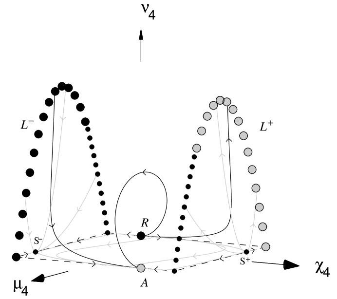
Figure 12: Phase portrait of the system (4.34)-(4.37) for $\Lambda_{\rm M}<0$ with $\rho=0$ and $K<0$. Note that $L^{+}$ and $L^{-}$ represent line of equilibrium points. See also caption to Fig. 1.

4.4.2 Qualitative Analysis of the Four-Dimensional System

The invariant set $K=0$ is discussed in Section 4.3.1 (see Fig. 10). The function $\mu_{4}/\sqrt{\nu_{4}}$ is monotonically increasing, and so there are no recurring or periodic orbits. The asymptotic behaviour is identical to that described in Section 4.3.3.

5 Discussion

In this paper, we have presented a complete qualitative analysis for the isotropic curvature string cosmologies derived from the effective action (2.10) in the two cases where either $\Lambda=0$ or $\Lambda_{\rm M}=0$ (the cases where both terms are non-zero is discussed in [25]). This was made possible by compactifying the phase space in terms of suitably defined variables. When $\Lambda_{\rm M}=0$, Eq. (2.10) represents the action for the NS–NS fields that arise in both the type II and heterotic string theories when an arbitrary central charge deficit is present. We identified the cosmological constant $\Lambda_{\rm M}$ with terms that arise in the RR sector of the massive type IIA supergravity theory when appropriate conditions apply.

The subset $\dot{\beta}=0$ corresponds to the class of spatially isotropic FRW universes with arbitrary spatial curvature. In the positively curved case, we have extended the work of Easter et al. [8], who performed a perturbation analysis on the static, closed FRW model to show that it was a late-time attractor. More generally, the models we have considered represent Bianchi type I, V and IX universes.

For each case, we have established the existence of monotonic functions which precludes the existence of recurrent or periodic orbits. Consequently, the early– and late–time behaviour of these models can be determined by analysing the nature of the equilibrium points/lines of the system. In all cases, the spatially flat dilaton–vacuum solutions $L^{\pm}$, given by Eq. (A.1), act as either early- or late-time attractors and, in many cases, act as both. Because these solutions lie in both the $\rho=0$ and $\tilde{K}=0$ invariant sets and contain neither a central charge deficit nor a non–zero $\Lambda_{\rm M}$ contribution, we may conclude that the shear and dilaton fields are dynamically dominant asymptotically. Furthermore, with the exception of the $\Lambda>0$, $\tilde{K}>0$ case, all early-time and late-time attracting sets lie in either the $\rho=0$ invariant set or the $\tilde{K}=0$ invariant set, and a majority of these sets lie in both.

Thus, we see a generic feature in which the curvature terms and the axion field are dynamically significant at intermediate times and are asymptotically negligible at early and late times. The exception to this generic behaviour is the $\Lambda>0$, $\tilde{K}>0$ case, where the generalized linear dilaton–vacuum solution (A.3), in which neither $\rho=0$ nor $\tilde{K}=0$, acts both as a repeller (for $\dot{\varphi}<0$) and as an attractor (for $\dot{\varphi}>0$). In these solutions, the variables $\rho$ and $\tilde{K}$ are proportional to the central charge deficit, $\Lambda$. Note that asymptotically $\dot{\alpha}=0$ (and $\dot{\beta}=0$) and hence these models are static.

When $\Lambda<0$, the central charge deficit is dynamically significant only at intermediate times, and is asymptotically negligible at early and late times. In fact, the only repelling and attracting sets in this instance are the dilaton–vacuum solutions. When $\Lambda>0$, the central charge deficit can be dynamically significant at both early and late times, and the corresponding solution is the generalized linear dilaton–vacuum solution (A.3), represented by the line $L_{1}$. When $\tilde{K}>0$, these solutions can be repelling ($\dot{\varphi}<0$) and attracting ($\dot{\varphi}>0$). When $\tilde{K}<0$, the endpoint of this line, $C$ (representing Eq. (A.4)) is a repeller.

When $\Lambda_{\rm M}>0$, the cosmological constant may play a significant rôle in the early and late time dynamics. For instance, although in the four-dimensional sets there are no repelling or attracting equilibrium points in which $\Lambda_{\rm M}$ is dynamically significant, we have found that the orbits which are attracted to the $\tilde{K}=0$ invariant set end in a heteroclinic sequence which interpolates between two dilaton–vacuum solutions (see Section 4.1.1, Fig. 7 and paper II). During this interpolation, the orbits repeatedly spend time in a region of phase space in which $\Lambda_{\rm M}$ is dynamically significant (the region $\lambda_{1}>0$ in Fig. 7), although most time is spent near the dilaton–vacuum saddle points where $\Lambda_{\rm M}$ is dynamically negligible. When $\Lambda_{\rm M}<0$, the cosmological constant can be dynamically significant at both early and late times, since solutions typically asymptote to the solution (A.7), where the shear and axion field are static. For the repelling and attracting sets of the $\Lambda_{\rm M}<0$ cases, the shear term is only dynamically significant when the cosmological constant is not, and vice versa.

The parameter $\beta$ measures the degree of anisotropy in the models. If we define isotropization by the condition $\dot{\beta}\rightarrow 0$ [26, 27], then we note that in general $\dot{\beta}\neq 0$ at the equilibrium points on the line $L^{\pm}$. Therefore, solutions asymptoting towards the sinks on these lines do not isotropize to the future. At all other equilibrium points, however, $\dot{\beta}=0$ and the corresponding appropriate string cosmologies therefore ‘isotropize’. This is an important result and a similar situation occurs in the time–reverse models. On the other hand, the question of isotropization of string cosmologies in a more general context remains an open question. Note that the shear in the models that we have discussed is essentially of Bianchi type I. In general relativity with a perfect fluid, it is known that Bianchi type I models isotropize whereas in general spatially–homogeneous models do not isotropize [26, 27]).

For the equilibrium points corresponding to the sinks on the line $L^{+}$, $\dot{\beta}^{2}\propto\dot{\varphi}^{2}$ ($\rho=\tilde{K}=0$), and so the energy densities of the modulus and dilaton fields are proportional to one another. Hence, the corresponding dilaton–vacuum solutions are “matter scaling” string cosmology solutions, which act as local attractors, similar to the matter scaling solutions in general relativistic scalar field cosmologies [28]. Finally, for every equilibrium point within these phase spaces, the scale factor of the corresponding exact solution is a power–law function of cosmic time, and therefore all of the corresponding exact solutions are self–similar [29].

The cases in which $\dot{\varphi}<0$ are related to a time reversal of the models discussed in the text. We have not explicitly considered these models here; however, the conclusions concerning isotropization are similar although the details of these models may be different (e.g., the rôle of sources and sinks can be interchanged).

In conclusion, therefore, we have established the qualitative properties of all the isotropic curvature string models discussed in the text by finding appropriate monotone functions. Typically, the curvature term is dynamically significant only at intermediate times and is asymptotically negligible. There are only two exceptions to this. The first corresponds to the case $\{\Lambda>0,\tilde{K}>0\}$, where the generalized linear dilaton–vacuum attractors and repellers have a non-negligible curvature. The second case is the $\{\Lambda_{\rm M}>0,\tilde{K}<0\}$ model in which the repeller $N$ represents the curvature–driven solution (A.6). Finally, we note that when $\Lambda_{\rm M}>0$ there exist heteroclinic sequences in the invariant set $\tilde{K}=0$. This implies that the qualitative behaviour associated with heteroclinic sequences is only valid for solutions which approach $\tilde{K}=0$.

Acknowledgments

APB is supported by Dalhousie University, AAC is supported by the Natural Sciences and Engineering Research Council of Canada (NSERC), and JEL is supported by the Royal Society.

Appendix A Equilibrium Points

In this Appendix, we present the analytical solutions to Eqs. (2.11)–(2.16) that represent all of the equilibrium points that arise in this paper.

The ‘dilaton-vacuum’ solutions correspond to solutions where the axion field is constant and cosmological constants vanish $(\Lambda=\Lambda_{\rm M}=\dot{\sigma}=0)$. In the spatially flat case $(\tilde{K}=0)$, they are power laws:

$$a = a_{*}\left|t\right|^{\pm h_{*}},$$

$$e^{\Phi} = e^{\Phi_{*}}\left|t\right|^{\pm 3h_{*}-1},$$

$$e^{\beta} = e^{\beta_{*}}\left|t\right|^{\pm\epsilon\sqrt{(1-3h_{*}^{2})/6}},$$

$$\sigma = \sigma_{*},$$

$$k = 0,$$ (A.1)

where $\{a_{*},\Phi_{*},\sigma_{*},\beta_{*},h_{*}\}$ are constants, $a\equiv e^{\alpha}$ is the averaged scale factor of the universe, the $\pm$ sign corresponds to the sign of $t$ and $\epsilon=\pm 1$. These solutions have a curvature singularity at $t=0$. Note that the shifted dilaton field (2.17) satisfies $\dot{\varphi}>0$ for $t<0$ and $\dot{\varphi}<0$ for $t>0$. The “$-$” branch of Eq. (A.1) corresponds to the line $L^{+}$ throughout this paper and the “$+$” branch corresponds to the line $L^{-}$.

Another solution which appears when both $\Lambda=\Lambda_{\rm M}=0$ and $\dot{\sigma}=0$ is the Milne form of flat space:

$$a = a_{*}\left(\pm t\right),$$

$$\Phi = \Phi_{*},$$

$$\beta = \beta_{*},$$

$$\sigma = \sigma_{*},$$

$$k = -a_{*}^{2},$$ (A.2)

where $\{a_{*},\Phi_{*},\beta_{*},\sigma_{*}\}$ are constants. The “$\pm$” sign corresponds to the sign of $t$. These solutions are labelled $S^{\pm}$ throughout the paper (note $S^{+}$ corresponds to $t<0$ and $S^{-}$ corresponds to $t>0$) and arise as saddle points.

There is a line of equilibrium points that arises when the central charge deficit, $\Lambda$, is included in the action (2.10). This class of solutions has the form

$$a = a_{*},$$

$$\Phi = \Phi_{*}+n\sqrt{\frac{6\Lambda}{2+n^{2}}}t,$$

$$\beta = \beta_{*},$$

$$\sigma = \sigma_{*}\pm\sqrt{\frac{2\left(1-n^{2}\right)}{3n^{2}}}\exp\left(-\Phi_{*}-n\sqrt{\frac{6\Lambda}{2+n^{2}}}t\right),$$

$$k = \frac{1-n^{2}}{2+n^{2}}\Lambda a_{*}^{2},$$ (A.3)

where $n\in[-1,1]$. The solution is static, but has non–trivial spatial curvature, dilaton and axion fields. These solutions are represented by the line $L_{1}$ in Section 3.1. In that Section they represent past attractors for $n\in(0,1]$ and future attractors for $n\in[-1,0)$. These solutions were found in [8] for $\dot{\varphi}>0$, where, by employing a perturbation analysis, they were found to be late-time attractors.

The endpoints of the line $L_{1}$ correspond to $n=\pm 1$. These represent spatially flat and isotropic solutions known as the ‘linear dilaton–vacuum’ solutions [24]. They are described by

$$a = a_{*},$$

$$\Phi = \Phi_{*}\pm\sqrt{2\Lambda}t,$$

$$\beta = \beta_{*},$$

$$\sigma = \sigma_{*},$$

$$k = 0,$$ (A.4)

where $\{a_{*},\Phi_{*},\beta_{*},\sigma_{*}\}$ are constants. The “$+$” solution is represented by the equilibrium point $C$ in Section 3.2.

We now consider the cosmologies where $\Lambda=0$ in the action (2.10). A spatially flat solution found previously in paper II is given by

$$a = a_{*}\left[\frac{\sqrt{3\Lambda_{\rm M}}}{4}|t|\right]^{\frac{1}{3}}$$

$$\Phi = \Phi_{*}-\ln\left[\frac{3\Lambda_{\rm M}}{16}t^{2}\right]$$

$$\beta = \beta_{*},$$

$$\sigma = \sigma_{*}\pm\frac{\sqrt{15}}{16}\Lambda_{\rm M}t^{2}$$

$$k = 0,$$ (A.5)

where $\{a_{*},\Phi_{*},\beta_{*},\sigma_{*}\}$ are arbitrary constants and time is defined over the interval $t<0$ ($\dot{\varphi}>0$) for the equilibrium point $S^{+}_{1}$ and $t>0$ ($\dot{\varphi}<0$) for the equilibrium point $S^{-}_{1}$ in Section 4.1.

There also exists a spatially curved, isotropic solution with a constant axion field. It is given by

$$a = \frac{1}{2}a_{*}\sqrt{\Lambda}_{\rm M}\left|t\right|,$$

$$\Phi = -\ln\left[\frac{1}{4}\Lambda_{\rm M}t^{2}\right],$$

$$\beta = \beta_{*}$$

$$\sigma = \sigma_{*},$$

$$k = -\frac{3}{4}\Lambda_{\rm M}a_{*}^{2}$$ (A.6)

where $\{a_{*},\beta_{*},\sigma_{*}\}$ are integration constants. The solution for $t<0$ is represented by the equilibrium point $N$ in Section 4.2.

For negative $\Lambda_{\rm M}$, there are also the solutions

$$a = \frac{a_{*}}{\sqrt{\pm 2t}},$$

$$\Phi = \Phi_{*}-\ln\left[-2\Lambda_{\rm M}t^{2}\right],$$

$$\beta = \beta_{*},$$

$$\sigma = \sigma_{*},$$

$$k = 0,$$ (A.7)

where $\{a_{*},\Phi_{*},\beta_{*},\sigma_{*}\}$ are constants. The $\pm$ sign corresponds to the the sign of $t$ and “$+$” solution corresponds to the repelling equilibrium point $R$ in Section 4.4, whereas the “$-$” solution corresponds to the attracting equilibrium point $A$ in that Section.

References

References

- [1] Green M B, Schwarz J H and Witten E 1987 Superstring Theory (Cambridge: Cambridge University Press)
- [2] Polchinski J 1998 String Theory (Cambridge: Cambridge University Press)
-
[3]
Veneziano G 1991 Phys. Lett. B265 287
Gasperini M and Veneziano G 1993 Astropart. Phys. 1 317 - [4] Billyard A P, Coley A A and Lidsey J E 1999 Phys. Rev. D59 123505
- [5] Billyard A P, Coley A A and Lidsey J E 1999 “Qualitative Analysis of Early Universe Cosmologies”, submitted to J. Math. Phys.
-
[6]
Goldwirth D S and Perry M J 1993
Phys. Rev. D49 5019
Behrndt K and Förste S 1994 Phys. Lett. B320 253
Behrndt K and Förste S 1994 Nucl. Phys. B430 441
Kaloper N, Madden R and Olive K A 1995 Nucl. Phys. B452 677 - [7] Kaloper N, Madden R and Olive K A 1996 Phys. Lett. B371 34
- [8] Easther R, Maeda K and Wands D 1996 Phys. Rev. D53 4247
- [9] MacCallum M A H 1973 Cargèse Lectures in Physics ed E Schatzman (New York: Gordan and Breach)
- [10] Ryan M P and Shepley L S 1975 Homogeneous Relativistic Cosmologies (Princeton, NJ: Princeton University Press)
- [11] Romans L J 1986 Phys. Lett. B169 374
- [12] Maharana J and Singh H 1997 Phys. Lett. B408 164
- [13] Bergshoeff E, De Roo M, Green M, Papadopoulos G and Townsend P 1996 Nucl. Phys. B470 113
-
[14]
Polchinski J and Witten E 1996 Nucl. Phys. B460 525
Polchinski and Strominger A 1996 Phys. Lett. B388 736
Green M, Hull C M and Townsend P 1996 Phys. Lett. B382 65
Hull C M 1998 J. High En. Phys. 9811 027
Meessen P and Ortin T 1999 Nucl. Phys. B541 195 -
[15]
Callan C G, Friedan D, Martinec E J and Perry M J 1985 Nucl. Phys.
B262 593
Fradkin E S and Tseytlin A A 1985 Phys. Lett. B158 316
Lovelace C 1986 Nucl. Phys. B273 416 - [16] Kaloper N, Kogan I I and Olive K A 1998 Phys. Rev. D57 7340
-
[17]
Shapere A, Trivedi S and Wilczek F 1991 Mod. Phys.
Lett. A6 2677
Sen A 1993 Mod. Phys. Lett. A8 2023 -
[18]
Lukas A, Ovrut B A and Waldram D 1997 Phys. Lett. B393 65
Lukas A, Ovrut B A and Waldram D 1997 Nucl. Phys. B495 365
Lü H, Mukherji S and Pope C N 1997 Phys. Rev. D55 7926
Lü H, Maharana J, Mukherji S and Pope C N 1998 Phys. Rev. D57 2219
Kaloper N 1997 Phys. Rev. D55 3394
Copeland E J, Lidsey J E and Wands D 1998 Phys. Rev. D57 625
Copeland E J, Lidsey J E and Wands D 1998 Phys. Rev. D58 043503 - [19] Scherk J and Schwarz J H 1979 Nucl. Phys. B153 61
- [20] Maharana J and Schwarz J H 1993 Nucl. Phys. B390 3
-
[21]
Buscher T H 1987 Phys. Lett. B194 59
Smith E and Polchinski J 1991 Phys. Lett. B263 59
Tseytlin A A 1991 Mod. Phys. Lett. A6 1721 - [22] Copeland E J, Lahiri A and Wands D 1994 Phys. Rev. D50 4868
- [23] Kar S, Maharana J and Singh H 1996 Phys. Lett. B374 43
-
[24]
Myers R C 1987 Phys. Lett. B199 371
Antoniadis I, Bachas C, Ellis J and Nanopoulos D V 1988 Phys. Lett. B211 393
Antoniadis I, Bachas C, Ellis J and Nanopoulos D V 1989 Nucl. Phys. B328 117 - [25] Billyard A P 1999 The Asymptotic Behaviour of Cosmological Models Containing Matter and Scalar Fields (Ph. D. Thesis, Dalhousie University)
- [26] Wainwright J and Ellis G F R 1997 Dynamical Systems in Cosmology (Cambridge: Cambridge University Press)
- [27] Collins C B and Hawking S W 1973 Astrophys. J. 180 317
-
[28]
Billyard A P, Coley A A,
van den Hoogen R J, Ibáñez J and Olasagasti I 1999 Scalar Field Cosmologies with Barotropic Matter: Models of Bianchi
class B (accepted to Class. Quantum Grav)
Copeland E J, Liddle A R and Wands D 1998 Phys. Rev. D57 4686 - [29] Maartens R and Maharaj S D 1986 Class. Quantum Grav. 3 1005