Renormalization
using
Domain Wall Regularization

1 Introduction

In the lattice world, it appears as if a new era is about to begin. [1, 2] The so-called “doubling problem” has become clarified, and the chirality of fermions can be controlled more efficiently than before. We may say a new regularization has been established in the lattice. In accordance with these great developments , the counterpart in the continuum is progressing. [3, 4, 5, 6, 7] There are two merits to such an approach. First, we can clearly understand the essential part of the new regularization, which is often hidden in the complexity of the discretized model. Second, we can compare the new regularization with the ordinary ones used to this time and apply it to various (continuum) field theories. The continuum version, at least, should explain the qualitative features of the lattice domain wall.

In the domain wall approach used to now, at least in the continuum approach, the gauge field in the fermion determinant is treated mainly as an external field. (For lattice model analysis, the gauge field quantum effect was examined, and the renormalizability was checked at the 1-loop level in Ref.[8].) Clearly, the situation is not satisfactory, because the gauge field is not treated as a quantum field and the general perspective regarding its use in (perturbative) quantum field theory has not been presented. Of course, the fermion determinant could be the most important among the other parts, but we must formulate the gauge field within the general setting in order to regard it as a new regularization in the field theory. This is what motivates the present work.

Recently, a new treatment has appeared in the continuum approach.[9, 10] The main idea is the following. The (regularization) ambiguity and the divergences of the fermion determinant can be resolved by introducing a “direction” into the system. This is based on an analogy to the well-defined determinant of the elliptic operator, which can be expressed in the form of a heat equation solution. Here we recall two facts: 1) the heat propagates in a fixed direction, that is, from high temperature to low temperature (as stipulated by the second law of the thermodynamics) and, generally, the heat equation describes such behaviour; 2) the famous procedure of introducing the heat equation into a general quantum system is the heat-kernel method.[11] The fermion determinant is very often examined using this method. (The anomaly is formulated from this point of view in Ref.[12].) We have shown that the above idea works well if we consider the 4 dimensional theory from the 1+4 dimensional space-time.

We summarize this new treatment in §2. New results regarding 2D and 4D QED Weyl anomalies are also presented. In §3, the renormalization procedure is introduced, and the (renormalized) effective action itself is used to derive anomalies. At this stage, we still keep the gauge field external, in order to make the explanation simple. In §4, we introduce the background field method[13, 14] and take into account the quantum effect of the gauge field as well as that of the fermion. We do the renormalization of the fermion self-energy explicitly. In §5, we present the complete formulation, combining the results of §§3 and 4. Finally, we point out that the domain wall regularization treats the fermion determinant part distinctly from the other parts.

2 Domain wall regularization

For a fermion system described by the quadratic form ${\cal L}={\bar{\psi}}{\hat{D}}\psi$, where the operator ${\hat{D}}$ satisfies

$$\gamma_{5}{\hat{D}}+{\hat{D}}\gamma_{5}=0{\quad,}\quad(\gamma_{5})^{2}=1{\quad,}$$ (1)

the fermion determinant (the effective action) can be expressed as

$$\ln\,Z[A_{\mu}]=-\int_{0}^{\infty}\frac{dt}{t}{\rm Tr\,}\left[{\frac{1}{2}}(1+i\gamma_{5})\exp\{it\gamma_{5}{\hat{D}}\}+{\frac{1}{2}}(1-i\gamma_{5})\exp\{-it\gamma_{5}{\hat{D}}\}\right]$$

$$=-\lim_{M\rightarrow 0}\int_{0}^{\infty}\frac{dt}{t}{\frac{1}{2}}(1-i\frac{\partial}{\partial(tM)}){\rm Tr\,}(G^{5M}_{+}(x,y;t)+G^{5M}_{-}(x,y;t))\ ,$$ (2)

where $t$ plays the role of the inverse temperature. Here $M$ is introduced as a regularization mass parameter [Regularization Prescription 1]. $M$ also plays the role of the source for $\gamma_{5}$. $A_{\mu}$ represents the background gauge field appearing in ${\hat{D}}$. We take $M>0$ for simplicity. $G^{5M}_{+}$ and $G^{5M}_{-}$ are defined as

$$G^{5M}_{+}(x,y;t)=<x|\exp\{+it\gamma_{5}({\hat{D}}+iM)\}|y>{\quad,}$$

$$G^{5M}_{-}(x,y;t)=<x|\exp\{-it\gamma_{5}({\hat{D}}+iM)\}|y>{\quad,}$$ (3)

and they satisfy the heat equations with the first derivative operator  $\mp i\gamma_{5}({\hat{D}}+iM)$. We call $G^{5M}_{+}$ and $G^{5M}_{-}$ the “(+)-domain” and “(-)-domain”, because in the extreme chiral limit (defined below) they have exponential distributions in the extra $t$-space, peaked at $t=0$ or $t=\infty$. . The key observation is that the heat equations turn out to be the 1+4 dimensional Minkowski Dirac equation after appropriate Wick rotations for $t$. For the system of 4 dimensional Euclidean QED, ${\hat{D}}=i\gamma_{\mu}(\partial_{\mu}+ieA_{\mu}),\ (\mu=1,2,3,4)$, they are

$$(i{}\hbox{\hskip 2.0pt\vtop{\hbox{}\vskip-24.0pt\hbox{$\backslash$}} \hskip-11.5pt$\partial$}-M)G^{5M}_{+}=ie{}\hbox{\hskip 2.0pt\vtop{\hbox{}\vskip-24.0pt\hbox{/}} \hskip-11.5pt$A$}G^{5M}_{+}{\quad,}\quad(X^{a})=(-it,x^{\mu}){\quad,}$$

$$(i{}\hbox{\hskip 2.0pt\vtop{\hbox{}\vskip-24.0pt\hbox{$\backslash$}} \hskip-11.5pt$\partial$}-M)G^{5M}_{-}=ie{}\hbox{\hskip 2.0pt\vtop{\hbox{}\vskip-24.0pt\hbox{/}} \hskip-11.5pt$A$}G^{5M}_{-}{\quad,}\quad(X^{a})=(+it,x^{\mu}){\quad,}$$ (4)

where ${}\hbox{\hskip 2.0pt\vtop{\hbox{}\vskip-24.0pt\hbox{/}} \hskip-11.5pt$A$}\equiv\gamma_{\mu}A_{\mu}(x)\ ,\ {}\hbox{\hskip 2.0pt\vtop{\hbox{}\vskip-24.0pt\hbox{$\backslash$}} \hskip-11.5pt$\partial$}\equiv\mathchar 28928\relax^{a}\frac{\partial}{\partial X^{a}}\ (a=0,1,2,3,4)$. Now, we can specify the above solution based on another key observation that the system should have a fixed direction [Regularization Prescription 2]. Generally, the solution of (4) is given by two ingredients (see a standard textbook, for example, Ref.[15]), 1) a free solution $G_{0}(X,Y)$, and 2) a propagator $S(X,Y)$ in the following form:

$$G^{5}_{M}(X,Y)=G_{0}(X,Y)+\int d^{5}Z\,S(X,Z)ie{}\hbox{\hskip 2.0pt\vtop{\hbox{}\vskip-24.0pt\hbox{/}} \hskip-11.5pt$A$}(z)G^{5}_{M}(Z,Y){\quad.}$$ (5)

This gives us the solution $G^{5}_{M}(X,Y)$ perturbatively with respect to the coupling $e$. As $S(X,Y)$, we should not use the Feynman propagator that has both retarded and advanced components. Instead we should use the retarded propagator for the (+)-domain and the advanced propagator for the (-)-domain:

$$\mbox{Symmetric retarded solution}\quad G^{5M}_{+}(\mbox{(+)-domain}):\quad$$

$$G_{0}(X,Y)=G^{p}_{0}(X,Y)-G^{n}_{0}(X,Y)\ ,$$

$$S(X,Y)=\theta(X^{0}-Y^{0})(G^{p}_{0}(X,Y)-G^{n}_{0}(X,Y))$$ (6)

$$\mbox{Symmetric advanced solution}\quad G^{5M}_{-}(\mbox{(-)-domain}):\quad$$

$$G_{0}(X,Y)=-G^{p}_{0}(X,Y)+G^{n}_{0}(X,Y)\ ,$$

$$S(X,Y)=\theta(Y^{0}-X^{0})(-G^{p}_{0}(X,Y)+G^{n}_{0}(X,Y))\ ,$$ (7)

where $G^{p}_{0}(X,Y)$ and $G^{n}_{0}(X,Y)$ are the positive and negative energy free solutions, respectively:

$$G^{p}_{0}(X,Y)\equiv-i\int\frac{d^{4}k}{(2\pi)^{4}}\mathchar 28938\relax_{+}(k)e^{-i{\tilde{K}}(X-Y)}{\quad,}\ \ \mathchar 28938\relax_{+}(k)\equiv\frac{M+{}\hbox{\hskip 2.0pt\vtop{\hbox{}\vskip-24.0pt\hbox{$\backslash$}} \hskip-11.5pt${\tilde{K}}$}}{2E(k)}{\quad,}$$

$$G^{n}_{0}(X,Y)\equiv-i\int\frac{d^{4}k}{(2\pi)^{4}}\mathchar 28938\relax_{-}(k)e^{+i{\bar{K}}(X-Y)}{\quad,}\ \ \mathchar 28938\relax_{-}(k)\equiv\frac{M-{}\hbox{\hskip 2.0pt\vtop{\hbox{}\vskip-24.0pt\hbox{$\backslash$}} \hskip-11.5pt${\bar{K}}$}}{2E(k)}{\quad,}$$ (8)

where $E(k)=\sqrt{k^{2}+M^{2}},({\tilde{K}}^{a})=(E(k),K^{\mu}=-k^{\mu}),({\bar{K}}^{a})=(E(k),-K^{\mu}=k^{\mu})$. Here, $k^{\mu}$ is the momentum in the 4 dimensional Euclidean space, and ${\tilde{K}}$ and ${\bar{K}}$ are the on-shell momenta, ${\tilde{K}}^{2}={\bar{K}}^{2}=M^{2}$, which correspond to the positive and negative energy states, respectively. The theta functions in (6) and (7) show the “directedness” of the solution. In this solution, both the positive and negative states propagate in the forward direction in the (+)-domain, while they both propagate in the backward direction in the (-)-domain. We call (6) and (7) “symmetric solutions”. (They are “symmetric” in the sense that the positive and negative energy parts are equally mixed. Compare them with the chiral “solution” presented below. ) The above solutions satisfy the following boundary conditions:

$$G^{5M}_{+}\mbox{(Retarded)}\rightarrow-i\gamma_{5}\delta^{4}(x-y)\ \mbox{as}\ M(X^{0}-Y^{0})\rightarrow+0\ ,$$

$$G^{5M}_{-}\mbox{(Advanced)}\rightarrow+i\gamma_{5}\delta^{4}(x-y)\ \mbox{as}\ M(X^{0}-Y^{0})\rightarrow-0\ .$$ (9)

In this procedure, we naturally notice the following attractive choice of $G_{0}(X,Y)$ and $S(X,Y)$:

$$\mbox{Retarded chiral "solution"}\quad G^{5M}_{+}(\mbox{(+)-domain}):\quad$$

$$G_{0}(X,Y)=G^{p}_{0}(X,Y){\quad,}\quad S(X,Y)=\theta(X^{0}-Y^{0})G^{p}_{0}(X,Y)$$ (10)

$$\mbox{Advanced chiral "solution"}\quad G^{5M}_{-}(\mbox{(-)-domain}):\quad$$

$$G_{0}(X,Y)=G^{n}_{0}(X,Y){\quad,}\quad S(X,Y)=\theta(Y^{0}-X^{0})G^{n}_{0}(X,Y){\quad.}$$ (11)

They also represent “directed” propagations, but do not satisfy (4). Instead they satisfy its chiral version in the large $M$ limit or the soft-momentum limit ($M/|k^{\mu}|\gg 1$),

$$(i{}\hbox{\hskip 2.0pt\vtop{\hbox{}\vskip-24.0pt\hbox{$\backslash$}} \hskip-11.5pt$\partial$}-M)G^{5M}_{+}=ieP_{+}{}\hbox{\hskip 2.0pt\vtop{\hbox{}\vskip-24.0pt\hbox{/}} \hskip-11.5pt$A$}G^{5M}_{+}+O(\frac{1}{M}){\quad,}\quad(X^{a})=(-it,x^{\mu}){\quad,}$$

$$(i{}\hbox{\hskip 2.0pt\vtop{\hbox{}\vskip-24.0pt\hbox{$\backslash$}} \hskip-11.5pt$\partial$}-M)G^{5M}_{-}=ieP_{-}{}\hbox{\hskip 2.0pt\vtop{\hbox{}\vskip-24.0pt\hbox{/}} \hskip-11.5pt$A$}G^{5M}_{-}+O(\frac{1}{M}){\quad,}\quad(X^{a})=(+it,x^{\mu}){\quad.}$$ (12)

The configuration in which the positive energy states propagate only in the forward direction of $X^{0}$ constitutes the ($+$)-domain, while the configuration in which the negative energy states propagate only in the backward direction constitutes the ($-$)-domain. As seen from their simple structure, the chiral “solutions” have some advantages (at least in concrete calculations). The validity of their use, however, is a subtle matter, because they are legitimate solutions of neither (4) nor its chiral version. Only in the extreme chiral limit ($M/|k|\gg 1$) do they correspond to the chiral operators ${\hat{D}}_{\pm}=i({\not\partial}+ieP_{\pm}{}\hbox{\hskip 2.0pt\vtop{\hbox{}\vskip-24.0pt\hbox{/}} \hskip-11.5pt$A$})$. We believe that their use is valid in the examination of global quantities or soft-momentum (infrared) properties. (This will be confirmed below.) The chiral “solutions” satisfy the boundary condition

$$i(G^{5M}_{+}(X,Y)-G^{5M}_{-}(X,Y))\rightarrow\gamma_{5}\delta^{4}(x-y)\ \mbox{as}\ M|X^{0}-Y^{0}|\rightarrow+0{\quad.}$$ (13)

As the final step of this regularization prescription, we take the following “double limits”[Regularization Prescription 3]:

$$\mbox{(i)}\quad\frac{|k^{\mu}|}{M}\leq 1{\quad,}\quad\mbox{(ii)}\quad Mt\ll 1{\quad,}$$

$$(\mbox{or}\quad|k^{\mu}|\leq M\ll\frac{1}{t}){\quad.}$$ (14)

These relations express the most characteristic point of this 1+4 dimensional regularization scheme. The condition (ii) comes from the usage of the regularization parameter $M$ in (2), whereas (i) comes from the necessity of controlling the chirality without destroying the system dynamics. Note that the roles of the regularization mass parameter $M$ for the $t$-axis and for the $x^{\mu}$-axis are different. The parameter $M$ restricts the configuration to the ultra-violet region ($t\ll M^{-1}$) in the “extra space” of $t$ and to the infra-red (surface) region in the real 4 dimensional space ($|k^{\mu}|\leq|M|$). (This situation regarding configuration restriction, by (i) and (ii), is discussed further in §§3 and 5.) In the concrete calculation, the condition (i) is taken into account not by performing $k^{\mu}$-integral with the cut-off $M$ but by using the analytic continuation in order to avoid breaking the gauge invariance[Regularization Prescription 3’].

The validity of the above regularization was confirmed in Refs.[9] and [10]. There we found properties analogous to those of the lattice domain wall: the domain wall configuration, the overlap Dirac operator, the condition on the regularization parameter $M$, etc.. We also confirmed that the chiral anomalies (for 2D QED, 4D QED and 2D chiral gauge theory) are correctly reproduced. One of the advantages of the present approach is the equal treatment of the chiral and Weyl anomalies. To understand the situation, let us apply the above regularization to the Weyl anomaly calculation. We first consider a simple model, 2D QED, for later purposes. It is given, using the chiral solution (13), as[10]

$$\delta_{\omega}\,\ln\,J_{W}=2i\lim_{M|X^{0}-Y^{0}|\rightarrow+0}{\rm Tr\,}\,\omega(x)\gamma_{5}(G^{5M}_{+}(X,Y)-G^{5M}_{-}(X,Y)){\quad,}$$

$$Tr\,\omega\gamma_{5}G^{5M}_{+}|_{AA}=\int^{X^{0}}_{0}dZ^{0}\int d^{2}Z\int^{Z^{0}}_{0}dW^{0}\int d^{2}W$$

$$\times{\rm Tr\,}\,\omega\gamma_{5}G^{p}_{0}(X,Z)ie{}\hbox{\hskip 2.0pt\vtop{\hbox{}\vskip-24.0pt\hbox{/}} \hskip-11.5pt$A$}(z)G^{p}_{0}(Z,W)ie{}\hbox{\hskip 2.0pt\vtop{\hbox{}\vskip-24.0pt\hbox{/}} \hskip-11.5pt$A$}(w)G^{p}_{0}(W,Y){\quad,}$$ (15)

(See Fig.1(i).) and similarly for $\mbox{Tr}\,\omega\gamma_{5}G^{5M}_{-}$ using $G^{n}_{0}$. After a standard calculation explained in Ref.[10], we obtain half of the correct result: $\delta_{\omega}\,\ln\,J_{W}=\omega(x){\frac{1}{2}}\frac{e^{2}}{\pi}{A_{\mu}}^{2}$. When we take the symmetric solution, we evaluate

$$\delta_{\omega}\,\ln\,J_{W}=i\lim_{M|X^{0}-Y^{0}|\rightarrow+0}{\rm Tr\,}\,\omega(x)\gamma_{5}(G^{5M}_{+}(X,Y)-G^{5M}_{-}(X,Y)){\quad,}$$

$$Tr\,\omega\gamma_{5}G^{5M}_{+}|_{AA}=\int^{X^{0}}_{0}dZ^{0}\int d^{2}Z\int^{Z^{0}}_{0}dW^{0}\int d^{2}W$$

$$\times{\rm Tr\,}\,\omega\gamma_{5}(G^{p}_{0}(X,Z)-G^{n}_{0}(X,Z))ie{}\hbox{\hskip 2.0pt\vtop{\hbox{}\vskip-24.0pt\hbox{/}} \hskip-11.5pt$A$}(z)(G^{p}_{0}(Z,W)-G^{n}_{0}(Z,W))$$

$$\times ie{}\hbox{\hskip 2.0pt\vtop{\hbox{}\vskip-24.0pt\hbox{/}} \hskip-11.5pt$A$}(w)(G^{p}_{0}(W,Y)-G^{n}_{0}(W,Y)){\quad.}$$ (16)

(See Fig.1(ii).) This reproduces the correct result: $\delta_{\omega}\,\ln\,J_{W}=\omega(x)\frac{e^{2}}{\pi}{A_{\mu}}^{2}$.

Fig. 1: Abelian gauge theory, $G^{5M}_{+}$, second order with respect to $A_{\mu}$ [$O(AA)$]: (i) the chiral “solution” and (ii) symmetric solution.

We have confirmed that similar situation exists in 4D Euclidean QED. The symmetric solution gives the correct Weyl anomaly: $\delta_{\omega}\ln J=\omega(x)\,\beta(e)F_{\mu\nu}F_{\mu\nu}\ ,\ \beta(e)=\frac{e^{2}}{12\pi^{2}}$, where $\beta(e)$ is the $\beta$-function in the renormalization group. The chiral “solution” gives one fourth of it.

Combined with the results for the chiral anomalies in Refs.[9] and [10], we conclude that the chiral “solution” gives $(1/2)^{d/2}$ (where $d$ is the spatial dimension) of the correct value of the anomaly coefficients both for the chiral anomaly and for the Weyl anomaly. The use of the chiral “solution” reduces the degree of freedom by half for each two dimensions. This phenomenon seems to contrast with the lattice’s doubling species phenomenon.

The use of the chiral “solution”, instead of the symmetric solution, should be limited to simple cases, such as the anomaly calculation. For the general case, in which local dynamics appears and we cannot ignore $O(1/M)$ in (12), we should use the symmetric solution.

3 Renormalization procedure

In this and the next sections, we develop a method for using the domain wall regularization in general field theory. We now introduce the counterterm action $\mathchar 28929\relax\mathchar 28928\relax[A]$ into the effective action $\mathchar 28928\relax[A]\equiv-\ln Z[A]$ as

$$\mathchar 28928\relax_{\mbox{bare}}[A]\equiv\mathchar 28928\relax[A]+\mathchar 28929\relax\mathchar 28928\relax[A]{\quad,}$$ (17)

in such a way that $\mathchar 28928\relax_{\mbox{bare}}$ becomes finite. Determining how to systematically define $\mathchar 28929\relax\mathchar 28928\relax$ and obtain the renormalization properties is the task of this section. Let us consider the simple model of 2D QED (Schwinger model) for this explanation. We consider the case in which $\mathchar 28929\relax\mathchar 28928\relax$ consists of local counterterms. From the power-counting analysis, we have

$$\mathchar 28929\relax\mathchar 28928\relax[A]=\int d^{2}x\left(c_{\mbox{div}}e^{2}{A_{\mu}}^{2}+c^{\prime}_{\mbox{div}}e\,\partial_{\mu}A_{\mu}+c^{\prime\prime}_{\mbox{div}}e\,\epsilon_{\mu\nu}\partial_{\mu}A_{\nu}\right){\quad,}$$ (18)

where $c_{\mbox{div}},c^{\prime}_{\mbox{div}}$ and $c^{\prime\prime}_{\mbox{div}},$ are some (divergent) constants to be systematically fixed. Now, we apply the following renormalization condition to $\mathchar 28928\relax_{\mbox{bare}}[A]$:

$$\left.\frac{\delta^{2}\mathchar 28928\relax_{\mbox{bare}}[A]}{\delta A_{\mu}(x)\delta A_{\nu}(y)}\right|_{A=0}=\frac{e^{2}}{\pi}\delta_{\mu\nu}\delta^{2}(x-y)\ ,\ \left.\frac{\delta\mathchar 28928\relax_{\mbox{bare}}[A]}{\delta A_{\mu}(x)}\right|_{A=0}=0{\quad.}$$ (19)

The first equation defines the renormalized coupling, and the second one guarantees stability.

In order to regularize the $t$-integral in $\mathchar 28928\relax[A]$, we introduce here two more regularization parameters, $\epsilon$ and $T$ ($0<\epsilon<t<T\ ,\ \epsilon\rightarrow+0\ ,\ T\rightarrow+\infty$) [Regularization Prescription 4]:

$$\mathchar 28928\relax[A]=-\ln\,Z[A]=$$

$$\lim_{T\rightarrow+\infty,\epsilon\rightarrow+0}\lim_{M\rightarrow 0}\int_{\epsilon}^{T}\frac{dt}{t}{\frac{1}{2}}(1-i\frac{\partial}{\partial(tM)}){\rm Tr\,}(G^{5M}_{+}(x,y;t)+G^{5M}_{-}(x,y;t)){\quad.}$$ (20)

$T$ is regarded as the length of the extra axis, and $\epsilon$ is the “regularized point” of the origin of the extra axis. It can also be regarded as the minimum unit of length (the ultraviolet cutoff). $T$ and $\epsilon$ regulate the infrared and ultraviolet behaviors, respectively. The relevant part is the order $A^{2}$ term,

$$G^{5M}_{+}|_{AA}=\int^{X^{0}}_{0}dZ^{0}\int^{Z^{0}}_{0}dW^{0}\int d^{2}Z\int d^{2}W(G^{p}_{0}(X,Z)-G^{n}_{0}(X,Z))ie{}\hbox{\hskip 2.0pt\vtop{\hbox{}\vskip-24.0pt\hbox{/}} \hskip-11.5pt$A$}(z)$$

$$(G^{p}_{0}(Z,W)-G^{n}_{0}(Z,W))ie{}\hbox{\hskip 2.0pt\vtop{\hbox{}\vskip-24.0pt\hbox{/}} \hskip-11.5pt$A$}(w)(G^{p}_{0}(W,Y)-G^{n}_{0}(W,Y))$$

$$=\int^{X^{0}}_{0}dZ^{0}\int^{Z^{0}}_{0}dW^{0}\int d^{2}z\int d^{2}w\int\frac{d^{2}k}{(2\pi)^{2}}\frac{d^{2}l}{(2\pi)^{2}}\frac{d^{2}q}{(2\pi)^{2}}$$

$$\times(-i)(\mathchar 28938\relax_{+}(k)e^{-iE(k)(X^{0}-Z^{0})}-\mathchar 28938\relax_{-}(k)e^{iE(k)(X^{0}-Z^{0})})ie{}\hbox{\hskip 2.0pt\vtop{\hbox{}\vskip-24.0pt\hbox{/}} \hskip-11.5pt$A$}(z)$$

$$\times(-i)(\mathchar 28938\relax_{+}(l)e^{-iE(l)(Z^{0}-W^{0})}-\mathchar 28938\relax_{-}(L)e^{iE(l)(Z^{0}-W^{0})})ie{}\hbox{\hskip 2.0pt\vtop{\hbox{}\vskip-24.0pt\hbox{/}} \hskip-11.5pt$A$}(w)$$

$$\times(-i)(\mathchar 28938\relax_{+}(q)e^{-iE(q)(W^{0}-Y^{0})}-\mathchar 28938\relax_{-}(q)e^{iE(q)(W^{0}-Y^{0})})e^{-ik(x-z)-il(z-w)-iq(w-y)}\ .$$ (21)

(See Fig.1(ii).) Evaluating the above equation and the similar one for $G^{5M}_{-}|_{AA}$, we obtain

$$\mathchar 28928\relax[A]|_{AA}=\lim_{T\rightarrow+\infty,\epsilon\rightarrow+0}\frac{e^{2}}{\pi}\ln\frac{T}{\epsilon}\times\int d^{2}x{A_{\mu}}^{2}{\quad.}$$ (22)

From the renormalization condition (19), we obtain

$$c_{\mbox{div}}=-\frac{1}{\pi}\ln\frac{T}{\epsilon}+\frac{1}{2\pi}{\quad.}$$ (23)

We now check above result by calculating the Weyl and chiral anomalies directly from the effective action. (In (15) and (16) of this paper, and in Ref.[10], anomalies are obtained from Jacobians.) The Weyl anomaly is obtained from the scale transformation of $\epsilon$ (or $T$),

$$\epsilon^{\prime}=e^{\mathchar 28929\relax}\epsilon=\epsilon+\mathchar 28929\relax\cdot\epsilon+O(\mathchar 28929\relax^{2}){\quad,}$$

$$\delta\mathchar 28928\relax_{\mbox{bare}}=\delta\,[c_{\mbox{div}}e^{2}\int d^{2}x{A_{\mu}}^{2}]=\mathchar 28929\relax\times\frac{e^{2}}{\pi}\int d^{2}x{A_{\mu}}^{2}{\quad,}$$ (24)

which agrees with the known result. The chiral anomaly is obtained by the variation of $A_{\mu}$, $\delta{}\hbox{\hskip 2.0pt\vtop{\hbox{}\vskip-24.0pt\hbox{/}} \hskip-11.5pt$A$}=-\frac{1}{e}{\not\partial}\alpha\cdot\gamma_{5}$, for $\mathchar 28928\relax_{\mbox{bare}}[A]$ :

$$\frac{\delta\mathchar 28928\relax_{\mbox{bare}}[A]}{\delta\alpha(x)}=+\frac{i}{\pi}e\epsilon_{\mu\nu}\partial_{\mu}A_{\nu}{\quad.}$$ (25)

Thus, both Weyl and chiral anomalies are correctly reproduced. Note that the chiral anomaly derived from the Jacobian in Ref. [9] comes from the $O(A)$-part of $G^{5M}_{\pm}$, whereas that derived here from the effective action comes from the $O(A^{2})$-part. (As for the Weyl anomaly, the results obtained from both approaches come from $O(A^{2})$-part.)

We conclude this section by listing all regularization parameters introduced and comparing them with the situation in lattice. We have introduced three parameters $M,T$ and $\epsilon$. They should satisfy the following relations with two configuration variables, the 4-momentum $k^{\mu}$ and the inverse-temperature $t$ :

$$|k^{\mu}|\leq M\ll\frac{1}{t}{\quad,}\quad\frac{1}{T}<\frac{1}{t}<\frac{1}{\epsilon}{\quad,}\quad\frac{1}{T}\ll\frac{1}{\epsilon}{\quad.}$$ (26)

In the above, we clearly see an important feature of the parameter $M$. Among the three relations above, the latter two are rather familiar. (The UV cut-off scale is $\epsilon$, while the IR cut-off scale is $T$.) The interesting one is the first. Before the appearance of domain wall regularization, we do not know of such a regularization parameter that depends on the configuration ( specified by $k^{\mu}$ and $t$ in the present case) in this way. In the conclusion of this paper, we point out another important character of the present regularization, which is obtained from the result above and that of the next section. In the lattice domain wall case, four parameters are introduced: $m_{0},a,L_{s},l$.[18] The correspondence with the present case is as follows:

present paper Ref.[18]

$$M \leftrightarrow m_{0}\ (\mbox{1+4 dim fermion mass}),$$

$$\epsilon \leftrightarrow a\ (\mbox{lattice spacing}),$$

$$\frac{T}{\epsilon} \leftrightarrow L_{s}\ (\mbox{the total site number along the extra axis}),$$

$$T \leftrightarrow l\ (\mbox{physical extent of one direction of the 4 dimensional box}).$$

The one extra parameter in the lattice comes from the fact that the extra space is treated independently of the 4 dimensional space. It is adopted in the ordinary domain wall formulation, whereas the present one treats the extra space as the space of the inverse temperature, which appears in expressing the determinant. In Ref.[18], the 4 dimensional fermion mass $m_{f}$ is also introduced. In such a case, we also introduce the mass parameter. (See Ref.[10])

4 General treatment of renormalization

To this point, we have discussed only the fermion determinant for the external gauge field. In order for this approach to be regarded as an alternative new regularization for general field theories, the quantum treatment of the gauge fields should also be described. We devote this section to this task.

The present approach quite naturally fits in the background field method.[13, 14] We explain it by again taking 4D Euclidean QED as an example. The quantum effects of both the gauge (photon) field and the fermion are taken into account. We consider the massive fermion,

$${\cal L}[\psi,{\bar{\psi}},A]=i{\bar{\psi}}\{\gamma_{\mu}(\partial_{\mu}+ieA_{\mu})+im\}\psi-\frac{1}{4}{F_{\mu\nu}}^{2}-{\frac{1}{2}}(\partial_{\mu}A_{\mu})^{2}{\quad,}$$ (28)

where the Feynman gauge is taken. According to the general theory of the background field method, complete physical information is contained in the following background effective action:

$$e^{-\mathchar 28928\relax[\chi,{\bar{\chi}},A]}=\int{\cal D}a_{\mu}{\cal D}\psi{\cal D}{\bar{\psi}}\exp\left[-\int d^{4}x\{{\cal L}[\chi+\psi,{\bar{\chi}}+{\bar{\psi}},A+a]\right.$$

$$\left.-\frac{\delta{\cal L}[\mathchar 28936\relax]}{\delta\mathchar 28936\relax^{i}}\phi^{i}-{\cal L}[\chi,{\bar{\chi}},A]\}\right]$$

$$=\int{\cal D}a_{\mu}{\cal D}\psi{\cal D}{\bar{\psi}}\exp\left[-\int d^{4}x\{\,{\cal L}_{2}[\psi,{\bar{\psi}},a]+{\cal L}_{3}[\psi,{\bar{\psi}},a]\,\}\right]$$

$${\cal L}_{2}[\psi,{\bar{\psi}},a;\chi,{\bar{\chi}},A]=i{\bar{\psi}}\{\gamma_{\mu}(\partial_{\mu}+ieA_{\mu})+im\}\psi-{\frac{1}{2}}(\partial_{\mu}a_{\nu})^{2}-e({\bar{\psi}}{}\hbox{\hskip 2.0pt\vtop{\hbox{}\vskip-24.0pt\hbox{/}} \hskip-10.5pt$a$}\chi+{\bar{\chi}}{}\hbox{\hskip 2.0pt\vtop{\hbox{}\vskip-24.0pt\hbox{/}} \hskip-10.5pt$a$}\psi){\quad,}$$

$${\cal L}_{3}[\psi,{\bar{\psi}},a]=-e{\bar{\psi}}{}\hbox{\hskip 2.0pt\vtop{\hbox{}\vskip-24.0pt\hbox{/}} \hskip-10.5pt$a$}\psi{\quad.}$$

(29)

Here, the fields $(\mathchar 28936\relax_{i})=(\chi,{\bar{\chi}},A_{\mu})$ are the background fields, and $(\phi_{i})=(\psi,{\bar{\psi}},a_{\mu})$ are the quantum fields. We note that the term ${\cal L}_{3}=-e{\bar{\psi}}{}\hbox{\hskip 2.0pt\vtop{\hbox{}\vskip-24.0pt\hbox{/}} \hskip-10.5pt$a$}\psi$ is the third order in the quantum fields and contributes to orders of 2-loops and higher. Terms in ${\cal L}_{2}$ are all second order and contribute to only the 1-loop order. Among them, the two terms $-e{\bar{\psi}}{}\hbox{\hskip 2.0pt\vtop{\hbox{}\vskip-24.0pt\hbox{/}} \hskip-10.5pt$a$}\chi$ and $-e{\bar{\chi}}{}\hbox{\hskip 2.0pt\vtop{\hbox{}\vskip-24.0pt\hbox{/}} \hskip-10.5pt$a$}\psi$ are off-diagonal with respect to the quantum fields.

In order to diagonalize the 1-loop part, we redefine the quantum fields as $\psi^{\prime}=\psi+\mathchar 28929\relax\psi,{\bar{\psi}}^{\prime}={\bar{\psi}}+\mathchar 28929\relax{\bar{\psi}},a_{\mu}^{\prime}=a_{\mu}+\mathchar 28929\relax a_{\mu}$. Here we choose $\mathchar 28929\relax\psi,\mathchar 28929\relax{\bar{\psi}}$ and $\mathchar 28929\relax a_{\mu}$ to be linear with respect to the quantum fields in order to maintain the loop-order structure. We require the 1-loop part, ${\cal L}_{2}[\psi,{\bar{\psi}},a]$, to be equal to

$$i{\bar{\psi}}^{\prime}\{\gamma_{\mu}(\partial_{\mu}+ieA_{\mu})+im\}\psi^{\prime}-{\frac{1}{2}}(\partial_{\mu}{a_{\nu}}^{\prime})^{2}{\quad.}$$ (30)

Then $\mathchar 28929\relax\psi$ and $\mathchar 28929\relax{\bar{\psi}}$ should satisfy

$$\mathchar 28929\relax{\bar{\psi}}(-i{\overleftarrow{{\not\partial}}}-e{}\hbox{\hskip 2.0pt\vtop{\hbox{}\vskip-24.0pt\hbox{/}} \hskip-11.5pt$A$}-m)=-e{\bar{\chi}}{}\hbox{\hskip 2.0pt\vtop{\hbox{}\vskip-24.0pt\hbox{/}} \hskip-10.5pt$a$}{\quad,}$$

$$(i{\not\partial}-e{}\hbox{\hskip 2.0pt\vtop{\hbox{}\vskip-24.0pt\hbox{/}} \hskip-11.5pt$A$}-m)\mathchar 28929\relax\psi=-e{}\hbox{\hskip 2.0pt\vtop{\hbox{}\vskip-24.0pt\hbox{/}} \hskip-10.5pt$a$}\chi{\quad.}$$ (31)

From this, we know that $\mathchar 28929\relax\psi$ and $\mathchar 28929\relax{\bar{\psi}}$ are proportional to the vector quantum field $a_{\mu}$ and begin from order $e$. Then $\mathchar 28929\relax a_{\mu}$ satisfies

$$\int d^{4}x\{{\frac{1}{2}}(\partial_{\mu}a_{\nu}+\partial_{\mu}(\mathchar 28929\relax a_{\nu}))^{2}-{\frac{1}{2}}(\partial_{\mu}a_{\nu})^{2}\}=\int d^{4}x\{-{\frac{1}{2}}e\,\mathchar 28929\relax{\bar{\psi}}{}\hbox{\hskip 2.0pt\vtop{\hbox{}\vskip-24.0pt\hbox{/}} \hskip-10.5pt$a$}\chi-{\frac{1}{2}}e\,{\bar{\chi}}{}\hbox{\hskip 2.0pt\vtop{\hbox{}\vskip-24.0pt\hbox{/}} \hskip-10.5pt$a$}\mathchar 28929\relax\psi\}\ ,$$

(32)

where the relations (31) have been used. Then, we see that the solution $\mathchar 28929\relax a_{\mu}$ is obtained as the expansion in the coupling $e$, beginning from order $e^{2}$. [The RHS of (32) begins from order of $e^{2}$.] We have

$$\mathchar 28929\relax a_{\mu}=e^{2}X^{(2)}_{\mu}+e^{3}X^{(3)}_{\mu}+O(e^{4}){\quad.}$$ (33)

Assuming $a_{\nu}\partial_{\mu}X^{(2)}_{\nu}$ damps sufficiently rapidly at the boundary $|x_{\mu}|=\infty$, $X^{(2)}_{\mu}$ satisfies the equation

$$\partial^{2}X^{(2)}_{\mu}=\frac{1}{2e}({\bar{\chi}}\gamma_{\mu}\mathchar 28929\relax\psi|_{e}+\mathchar 28929\relax{\bar{\psi}}|_{e}\gamma_{\mu}\chi){\quad.}$$ (34)

Here,“$|_{e}$” represents the operation of extracting the first order part in $e$. Therefore the RHS is 0-th order in $e$.

Equation (31) can be perturbatively solved by requiring the natural condition that $\mathchar 28929\relax\psi$ and $\mathchar 28929\relax{\bar{\psi}}$ vanish when the quantum fields vanish, $(a_{\mu},\psi,{\bar{\psi}})=0$. This gives

$$\mathchar 28929\relax\psi(x)=-\int d^{4}y\,S^{A}(x-y)e{}\hbox{\hskip 2.0pt\vtop{\hbox{}\vskip-24.0pt\hbox{/}} \hskip-10.5pt$a$}(y)\chi(y)=-\int d^{4}y\,S(x-y)e{}\hbox{\hskip 2.0pt\vtop{\hbox{}\vskip-24.0pt\hbox{/}} \hskip-10.5pt$a$}(y)\chi(y)+O(e^{2})\ ,$$

$$\mathchar 28929\relax{\bar{\psi}}(x)=-\int d^{4}y\,e{\bar{\chi}}(y){}\hbox{\hskip 2.0pt\vtop{\hbox{}\vskip-24.0pt\hbox{/}} \hskip-10.5pt$a$}(y){\bar{S}}^{A}(x-y)=-\int d^{4}y\,e{\bar{\chi}}(y){}\hbox{\hskip 2.0pt\vtop{\hbox{}\vskip-24.0pt\hbox{/}} \hskip-10.5pt$a$}(y){\bar{S}}(x-y)+O(e^{2})\ ,$$ (35)

where $S^{A},{\bar{S}}^{A},S$ and ${\bar{S}}$ are defined by

$$(i{\not\partial}-e{}\hbox{\hskip 2.0pt\vtop{\hbox{}\vskip-24.0pt\hbox{/}} \hskip-11.5pt$A$}-m)S^{A}(x-y)=\delta^{4}(x-y)\ ,\ (i{\not\partial}-m)S(x-y)=\delta^{4}(x-y)\ ,$$

$${\bar{S}}^{A}(x-y)(-i{\overleftarrow{{\not\partial}}}-e{}\hbox{\hskip 2.0pt\vtop{\hbox{}\vskip-24.0pt\hbox{/}} \hskip-11.5pt$A$}-m)_{y}=\delta^{4}(x-y)\ ,\ {\bar{S}}(x-y)(-i{\overleftarrow{{\not\partial}}}-m)_{y}=\delta^{4}(x-y)\ .$$ (36)

Here $S^{A}(x-y)$ and ${\bar{S}}^{A}(x-y)$ are background dependent propagators. All these propagators are (4D) Euclidean ones, and there is no ambiguity in the choice of boundary conditions.

The path-integral expression (29) can be rewritten by using redefined quantum fields using the measure change

$${\cal D}a_{\mu}{\cal D}\psi{\cal D}{\bar{\psi}}=J\times{\cal D}{a_{\nu}}^{\prime}{\cal D}\psi^{\prime}{\cal D}{\bar{\psi}}^{\prime}{\quad,}\quad J\equiv\frac{\partial(a_{\mu},\psi,{\bar{\psi}})}{\partial({a_{\nu}}^{\prime},\psi^{\prime},{\bar{\psi}}^{\prime})}{\quad.}$$ (37)

Since we keep the linear relation in the choice of the redefined quantum fields, the Jacobian $J$ does not depend on quantum fields:

$$e^{-\mathchar 28928\relax[\chi,{\bar{\chi}},A]}=J\times\int{\cal D}{a_{\mu}}^{\prime}{\cal D}\psi^{\prime}{\cal D}{\bar{\psi}}^{\prime}\exp[-\int d^{4}x\{i{\bar{\psi}}^{\prime}\gamma_{\mu}(\partial_{\mu}+ieA_{\mu}+im)\psi^{\prime}$$

$$-{\frac{1}{2}}(\partial_{\mu}{a_{\nu}}^{\prime})^{2}+\mbox{cubic terms w.r.t. quantum fields}\}]{\quad,}$$ (38)

The 1-loop part in the integrand is the quantity discussed in §2 for the case $m=0$ ( §7 of Ref.[10] treats the case $m\neq 0$). Up to the lowest nontrivial order, $J$ is obtained as

$$J^{-1}=\frac{\partial({a_{\mu}}^{\prime},\psi^{\prime},{\bar{\psi}}^{\prime})}{\partial(a_{\nu},\psi,{\bar{\psi}})}=\det(\delta_{\mu\nu}\delta^{4}(x-y)+e^{2}\frac{\delta X^{(2)}_{\mu}(x)}{\delta a_{\nu}(y)}+O(e^{3}))$$

$$=\exp\,[e^{2}{\rm Tr\,}\,(\frac{\delta X^{(2)}_{\mu}(x)}{\delta a_{\nu}(y)})+O(e^{3})]\ ,$$

$$\ln J=e^{2}{\rm Tr\,}_{x=z,\mu=\nu}\int d^{4}yD(x-y){\bar{\chi}}(y)\gamma_{\mu}S(y-z)\gamma_{\nu}\chi(z)+O(e^{3}){\quad.}$$ (39)

This corresponds to the 1-loop part for the fermion self-energy. (See Fig. 2.)

Fig. 2: Fermion self-energy.

Indeed, the quantum effect of the gauge field is taken into account. (Demonstrating this was the original motivation of the present work.) Because the Jacobian is decoupled from the main integral part, the regularization for the divergences in (39) can be done independently of the regularization parameter $M$ introduced in Sec.2. The quantity to be regularized in Sec.2 was $\det({\not\partial}+ie{}\hbox{\hskip 2.0pt\vtop{\hbox{}\vskip-24.0pt\hbox{/}} \hskip-11.5pt$A$})$, while the Jacobian above is roughly $\det(1+e^{2}\frac{1}{\partial^{2}}{\bar{\chi}}\frac{1}{{\not\partial}}\chi)=\det(\partial^{2}+e^{2}{\bar{\chi}}\frac{1}{{\not\partial}}\chi)/\det\partial^{2}$. Both quantities are divergent, but the presence of “$\partial^{2}$” inside the determinant in the latter quantity causes no chiral problem. [There is no ambiguity in determining the divergent quantity $\det(\partial^{2}+\cdots)$ because it can be expressed as the heat equation (not the Dirac equation ) in 1+4 dimension. (See §2 of Ref.[10].) ] The (momentum) integral, corresponding to “trace” in (39), is evaluated in the usual way, as described in standard field theory textbooks.

We explain the effective action calculation in the coordinate space in more detail. We have

$$\ln J|_{e^{2}}=e^{2}\int d^{4}y\int d^{4}xD(x-y){\bar{\chi}}(y)\gamma_{\mu}S(y-x)\gamma_{\mu}\chi(x)$$

$$=e^{2}\int d^{4}y\int d^{4}xD(x-y){\bar{\chi}}(y)\gamma_{\mu}S(y-x)\gamma_{\mu}\{\chi(y)+(x-y)^{\mu}\partial_{\mu}\chi|_{y}+\cdots\}$$

$$\equiv\mathchar 28928\relax_{{\bar{\chi}}\chi}+\mathchar 28928\relax_{{\bar{\chi}}\partial\chi}+\cdots{\quad,}$$

(40)

where $\chi(x)$ is Taylor expanded around $y$, and each expanded part is defined by $\mathchar 28928\relax_{{\bar{\chi}}\chi}$,$\mathchar 28928\relax_{{\bar{\chi}}\partial\chi}$,$\cdots$. Here $D(x)$ comes from the photon propagation and is defined by $\partial^{2}D(x)=\delta^{4}(x)$. The usual integral calculation gives the (ultra) divergent parts as

$$\mathchar 28928\relax_{{\bar{\chi}}\chi}=\frac{e^{2}}{2\pi^{2}}m\ln\frac{T}{\epsilon}\times\int d^{4}y\,{\bar{\chi}}(y)\chi(y)+\mbox{finite term}{\quad,}$$

$$\mathchar 28928\relax_{{\bar{\chi}}\partial\chi}=-\frac{e^{2}}{8\pi^{2}}\ln\frac{T}{\epsilon}\times\int d^{4}y\,i{\bar{\chi}}(y){\not\partial}\chi(y)+\mbox{finite term}{\quad,}$$ (41)

where we take the region of the momentum integral as $\frac{1}{T}<|k_{\mu}|<\frac{1}{\epsilon}$, where $T$ and $\epsilon$ were introduced in §3 as the infrared and ultraviolet cutoffs. Here, we find the fermion part of the counter action as [the gauge part is given in (18) for 2D QED]

$$\mathchar 28929\relax\mathchar 28928\relax[\chi,{\bar{\chi}}]=\int d^{4}y\,\left\{\frac{e^{2}}{2\pi^{2}}m\ln\frac{T}{\epsilon}\times{\bar{\chi}}(y)\chi(y)-\frac{e^{2}}{8\pi^{2}}\ln\frac{T}{\epsilon}\times i{\bar{\chi}}(y){\not\partial}\chi(y)\right\}\ ,$$ (42)

which is introduced in order to cancel the divergences of (41). The quantity $\mathchar 28929\relax\mathchar 28928\relax$ is “absorbed” by the mass renormalization $m+\mathchar 28929\relax m$ and the wave function renormalization of the fermion $\sqrt{Z_{2}}$ as follows:

$$\mathchar 28929\relax\mathchar 28928\relax[\chi,{\bar{\chi}},A]\equiv\int d^{4}x\mathchar 28929\relax{\cal L}[\chi,{\bar{\chi}},A]{\quad,}$$

$${\cal L}[\chi,{\bar{\chi}},A;e,m]+\mathchar 28929\relax{\cal L}[\chi,{\bar{\chi}},A]={\cal L}[\sqrt{Z_{2}}\chi,\sqrt{Z_{2}}{\bar{\chi}},\sqrt{Z_{3}}A;e+\mathchar 28929\relax e,m+\mathchar 28929\relax m]{\quad,}$$

$$m+\mathchar 28929\relax m=m(1-\frac{3e^{2}}{8\pi^{2}}\ln\frac{T}{\epsilon}){\quad,}\quad\sqrt{Z_{2}}=1-\frac{e^{2}}{16\pi^{2}}\ln\frac{T}{\epsilon}{\quad.}$$

(43)

Note in particular that the mass is renormalized in the multiplicative manner, as expected.

5 Discussion and conclusion

Combining the results of §§3 and 4, we present the final form of the renormalization prescription (taking 4D QED as an example) with the background field gauge:[14]

$$(\mathchar 28936\relax_{i})=(\chi,{\bar{\chi}},A):\ \mbox{Background fields}{\quad,}\quad(\phi_{i})=(\psi,{\bar{\psi}},a):\ \mbox{Quantum fields}{\quad,}$$

$${\cal L}[\chi,{\bar{\chi}},A;e,m]=i{\bar{\chi}}\gamma_{\mu}(\partial_{\mu}+ieA_{\mu}+im)\chi-\frac{1}{4}{F_{\mu\nu}}^{2}{\quad,}$$

$${\cal L}_{\mbox{gauge}}[a;\xi]=-\frac{1}{2\xi}(\partial_{\mu}a_{\mu})^{2}{\quad,}$$

$$e^{-\mathchar 28928\relax_{\mbox{bare}}[\mathchar 28936\relax]}=\int{\cal D}\phi\,\exp\left[-\int d^{4}x\{{\cal L}[\mathchar 28936\relax+\phi]+{\cal L}_{\mbox{gauge}}[a]+\mathchar 28929\relax{\cal L}[\mathchar 28936\relax+\phi]\right.$$

$$\left.-\frac{\delta}{\delta\mathchar 28936\relax^{i}}({\cal L}[\mathchar 28936\relax]+\mathchar 28929\relax{\cal L}[\mathchar 28936\relax])\phi^{i}-{\cal L}[\mathchar 28936\relax]-\mathchar 28929\relax{\cal L}[\mathchar 28936\relax]\}\right]{\quad.}$$

(44)

Here, the fermion determinant part only is regularized by the domain wall regularization of §2, while other parts are regularized by the cutoffs for the $t$-axis: $\epsilon<t<T(\mbox{or }\frac{1}{T}<|k_{\mu}|<\frac{1}{\epsilon})$. The background field gauge is chosen here and $\xi$ is the gauge parameter. $\mathchar 28929\relax{\cal L}$ is obtained in such a way that $\mathchar 28928\relax_{\mbox{bare}}$ becomes finite, satisfying some proper renormalization condition on the following quantities:

$$\left.\frac{\delta^{2}\mathchar 28928\relax_{\mbox{bare}}[\chi,{\bar{\chi}},A]}{\delta A_{\mu}(x)\delta A_{\nu}(y)}\right|_{\chi={\bar{\chi}}=A=0}\ ,\ \left.\frac{\delta^{2}\mathchar 28928\relax_{\mbox{bare}}[\chi,{\bar{\chi}},A]}{\delta\chi(x)\delta{\bar{\chi}}(y)}\right|_{\chi={\bar{\chi}}=A=0}\ ,\$$

$$\left.\frac{\delta^{3}\mathchar 28928\relax_{\mbox{bare}}[\chi,{\bar{\chi}},A]}{\delta A_{\mu}(x)\delta\chi(y)\delta{\bar{\chi}}(z)}\right|_{\chi={\bar{\chi}}=A=0}{\quad.}$$ (45)

In paticular, the fermion mass and the gauge coupling are normalized by the second and the third conditions, respectively. The renormalization parameters are obtained by

$${\cal L}[\chi,{\bar{\chi}},A;e,m]+\mathchar 28929\relax{\cal L}[\chi,{\bar{\chi}},A]={\cal L}[\sqrt{Z_{2}}\chi,\sqrt{Z_{2}}{\bar{\chi}},\sqrt{Z_{3}}A;e+\mathchar 28929\relax e,m+\mathchar 28929\relax m]{\quad.}$$ (46)

Comparing with the case in §4, we have the relation

$$\sqrt{Z_{3}}=\frac{1}{1+\frac{\mathchar 28929\relax e}{e}}{\quad,}$$ (47)

because the background gauge invariance is preserved. Some comments, in relation to the higher-loop structure, are in order. [14]

1. Generally, the terms in the Taylor expansion of $\mathchar 28929\relax{\cal L}$ play the role of subtracting sub-divergences in multi-loop diagrams. The proof of this point is largely based on the structure of the Taylor expansion.

2. From the viewpoint of the Taylor expansion, we compare the treatment of the gauge part in this section and §4. In §4, the gauge term $-{\frac{1}{2}}(\partial_{\mu}A_{\mu})^{2}$ is properly Taylor expanded in (29). Therefore, in this case, the subdivergence problem is manifestly solved. Contrastingly, the background field gauge adopted in this section, ${\cal L}_{\mbox{gauge}}$ in (44), is not Taylor expanded. The proof of the subdivergence cancellation is carried out by using the properties described in item 3, below. The superiority of (44) is that the effective action $\mathchar 28928\relax_{\mbox{bare}}$ is guaranteed to be gauge invariant.

3. In relation to the subdivergence problem mentioned above, at orders of 2-loops and higher, the gauge parameter and quantum fields suffer from the renormalization effect (i.e., the renormalization of “internal” quantities).

Through this analysis, the character of the domain wall regularization is revealed. The first point of note is the condition on the regularization parameters (26), as stated in §3. The second point is that the treatment of the fermion loop (determinant) is different from that of the other types of loops, which are irrelevant to the chiral problem. For the fermion loop, we do the calculation in the following order: 1) the momentum ($k^{\mu}$) integral in the region $|k^{\mu}|\leq M$ is evaluated for fixed $t$; 2) the procedure $Mt\ll 1$ is carried out; 3) the extra coordinate ($t$) integral is evaluated. Therefore, for each $t$-segment, the momentum region is suppressed as $|k_{\mu}|\leq M_{t}(\ll\frac{1}{t})$, where the subscript $t$ indicates a possible slight $t$ dependence. In order to show the restricted configuration region, we present a schematic chart of the momentum-integration region in a “phase space” ($|k^{\mu}|,t$). (See Fig.3.)

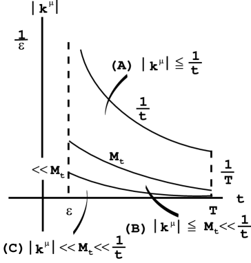
Fig. 3: The restricted regions of the momentum-integral in the “phase space” ($|k^{\mu}|,t$). All relations between parameters and the momentum are listed in (26). Three regions are shown: (A) [below the $t^{-1}$ line] the ordinary integral region; (B) [below the $M_{t}$ line] the domain wall regularization; (C) [far below the $M_{t}$ line] the extreme chiral region.

The present regularization considers the region below the $M_{t}$ line. For other types of loops, the corresponding region is suppressed as $|k_{\mu}|\leq\frac{1}{t}$. (In Fig.3, this is the region below the $t^{-1}$ line.) Two upper cut-offs have the relation $M_{t}\ll\frac{1}{t}$ from the requirement (26). It is expected that the final physical results are not affected by the different treatments, depending on the types of loops, of the momentum integrals as far as the low energy fermion and gauge bosons are concerned. (This situation is realised in the lattice numerical simulation.)

In the literature to this time, the domain wall has been investigated mainly with regard to the determinant calculation for the external gauge field. In the present paper, we have formulated it in the general field theory framework, using the background field method, where both fermions and (gauge) bosons are treated as quantum fields. We can calculate any term, in principle, of the effective action. We have explicitly carried out the renormalization of the fermion wave function and the fermion mass. We find that they agree with previous results.

Finally, we comment on the relation with the recently popular higher-dimensional approaches, such as the brane-world approach, Randall-Sundrum model, etc. They start from a higher-dimensional gravitational theory and consider a soliton configuration localized in the extra space. In this setting, the dimensional reduction from 5 dimensions to 4 dimensions takes place. In accordance with this, the mass hierarchy characterized by some exponential factor appears. This makes the model building based on this mechanism attractive. Contrastingly, the present approach starts from the 4 dimensions and for the purpose of the chiral regularization, we make use of its 5 dimensional Dirac equation. We suspect that both approaches do essentially the same thing, based on the following similar ingredients involved: 1) the domain wall configuration; 2) the exponentially damping or growing factors; 3) the chiral properties; 4) the scaling role played by the extra-space parameter or coordinate; 5) the fact that the regularization parameter $M$ in the present treatment appears to correspond to the parameter of (thickness)^-1 in the RS-model; 6) the fact that infrared-ultraviolet relation appears. The purpose of the higher-dimensional models is to find a theory beyond the standard model. This is different from the present purpose, namely, regularization of the fermion system. We can, however, find a common root in the paper of Callan and Harvey[20].

References

• [1] H.Neuberger,Talk at Chiral ’99,Sep.13-18,1999,National Taiwan Univ., “Overlap”,Chin.J.Phys.38(2000), 533.
• [2] M.Creutz,Comp.Phys.Comm.127(2000), 37,hep-lat/9904005.
• [3] R.Narayanan and H.Neuberger,Nucl. Phys. B412 (1994), 574.
• [4] R.Narayanan and H.Neuberger,Nucl. Phys. B443 (1995), 305.
• [5] S.Randjbar-Daemi and J.Strathdee,Nucl. Phys. B443 (1995), 386.
• [6] S.Randjbar-Daemi and J.Strathdee,Phys. Lett. B348 (1995), 543.
• [7] S.Randjbar-Daemi and J.Strathdee,Phys. Lett. B402 (1997), 134.
• [8] A.Yamada,Phys. Rev. D57 (1998), 1433.
• [9] S.Ichinose,Phys. Rev. D61 (2000), 055001, hep-th/9811094.
• [10] S.Ichinose,Nucl. Phys. B574 (2000), 719, hep-th/9908156.
• [11] J.Schwinger,Phys. Rev. D82 (1951), 664.
• [12] S.Ichinose and N.Ikeda,Phys. Rev. D53 (1996), 5932.
• [13] G. ’tHooft,Nucl. Phys. B62 (1973), 444.
• [14] S.Ichinose and M.Omote,Nucl. Phys. B203 (1982), 221.
• [15] J.D.Bjorken and S.D.Drell,Relativistic Quantum Mechanics (McGraw-Hill,New York,1964);Relativistic Quantum Fields (ibid.,1965).
• [16] R.Casana and S.A.Dias,Jour.Phys.G27(2001)1501, hep-th/0106057
• [17] E.Abdalla, M.C.B.Abdalla, and K.D.Rothe, 2 Dimensional Quantum Field Theory (World Scientific,Singapore,1991).
• [18] P.M.Vranas,Phys. Rev. D57 (1998), 1415.
• [19] Y.Shamir,Nucl. Phys. B406 (1993), 90.
• [20] C.G.Callan and J.A.Harvey,Nucl. Phys. B250 (1985), 427