Abstract

In these lectures we discuss the application of discrete light cone quantization (DLCQ) to supersymmetric field theories. We will see that it is possible to formulate DLCQ so that supersymmetry is exactly preserved in the discrete approximation. We call this formulation of DLCQ, SDLCQ and it combines the power of DLCQ with all of the beauty of supersymmetry. In these lecture we will review the application of SDLCQ to several interesting supersymmetric theories. We will discuss two dimensional theories with (1,1), (2,2) and (8,8) supersymmetry, zero modes, vacuum degeneracy, massless states, mass gaps, theories in higher dimensions, and the Maldacena conjecture among other subjects.

Introduction.

In the last decade there have been significant improvements in our understanding of gauge theories and important breakthroughs in the nonperturbative description of supersymmetric gauge theories [74, 75]. In the last few years various relations between string theory, brane theory and gauge fields [35, 2] have also emerged. While these developments give us some insight into strongly coupled gauge theories [75], they do not offer a direct method for non-perturbative calculations. In these lectures we discuss some recent developments in light cone quantization approaches to non-perturbative problems. We will see that these methods have the potential to expand our understanding of strongly coupled gauge theories in directions not previously available.

The original idea was formulated half of a century ago [32], but apart from several technical clarifications [63] it remained mostly undeveloped. The first change came in the mid 80–th when the Discrete Light Cone Quantization (DLCQ) was suggested as a practical way for calculating the masses and wavefunctions of hadrons [68]. Although the direct application of the method to realistic problems meets some difficulties (for review see [25]), DLCQ has been successful in studying various two dimensional models. Given the importance of supersymmetric theories, it is not surprising that light cone quantization was ultimately applied to such models [57, 20, 23]. Even in this early work the mass spectrum was shown to be supersymmetric in the continuum and a great deal of information about the properties of bound states in supersymmetric theories was extracted. However the straightforward application of DLCQ to the supersymmetric systems had one disadvantage: the supersymmetry was lost in the discrete formulation. The way to solve this problem was suggested in [64], where an alternative formulation of DLCQ was introduced. Namely it was noted that since the supercharge is the ”square root” of Hamiltonian one can define a new DLCQ procedure based on the supercharge. We will study this formulation (called SDLCQ) in these lectures.

These lectures have the following organization. In section 1 we introduce the basic concepts of DLCQ and SDLCQ. We also define the systems to be studied in the remaining lectures. We will concentrate our attention on two dimensional models with adjoint matter, several examples of such systems can be constructed from supersymmetric Yang–Mills theories in higher dimensions using dimensional reduction. In section 2 we address the problem of the DLCQ vacuum. In the continuum theory the light cone vacuum is very simple: it coincides with the usual Fock vacuum. This property is related to the decoupling between positive and negative frequency modes on the light cone and does not occur for equal time quantization. In DLCQ however one encounters the problem of zero modes which complicates the structure of vacuum and allows us to reproduce the correct vacuum degeneracy in certain theories. We continue to analyze zero modes in the section 3 and they are shown to play an important role in explaining the difference between DLCQ and SDLCQ regularization procedures.

Section 4 is devoted to the study of massless states. Our numerical analysis [64, 6, 11, 9] shows an important property of the mass spectrum for some supersymmetric theories. We find that unlike the QCD–like models [46], such systems appear to have a lot of massless bound states and in fact the supersymmetric $SU(\infty)$ gauge theory seems to have an infinite number of such states in the continuum limit. Since the states with zero mass dominate the partition function for low enough temperatures they deserve to be studied very carefully and in section 4 we analyze the structure of such states.

As we already mentioned in the beginning of this introduction, the relation between string theory and gauge fields has attracted a lot of attention in recent years. In particular it was conjectured [61] that one can extract some information about strongly coupled gauge theory from supergravity calculations. The problem however is that in the relevant regime usual field theoretic methods do not work, so it is hard to really test the conjecture. For two dimensional systems, however DLCQ gives solutions of the bound state problem which are valid beyond perturbation theory, so the results can be used to test the conjecture. We report the results of this first test in section 5. For realistic systems with eight supersymmetries we still don’t have enough computer power to compare the results with the supergravity predictions. The general techniques described in this section can also be used to calculate other correlation functions in the nonperturbative regime.

Finally in section 6 we make a first attempt to move beyond two dimensions. We present the general ideas for formulating SDLCQ in more than two dimensions. As an example we present the numerical results of SYM for the simplest case when only one transverse momentum mode is introduced.

1 Supersymmetric Yang–Mills Theory in the Light–Cone Gauge.

1.1 DLCQ and Its Supersymmetric Version.

In this work we will study the bound state problem for various supersymmetric matrix models in two dimensions. The examples of such models may be constructed by dimensional reduction of supersymmetric Yang–Mills theory in higher dimensions. In this subsection we will consider such reduction for three dimensional SYM. Before we begin the detailed analysis of the bound state problem for the specific systems it is worthwhile to summarize some basic ideas of Discrete Light Cone Quantization ( for a complete review see [25]).

Let us consider a general relativistic system in two dimensions. Usual canonical quantization of such a system means that one imposes certain commutation relations between coordinates and momenta at equal time. However as was pointed out by Dirac long ago [32] this is not the only possibility. Another scheme of quantization treats the light like coordinate $x^{+}=\frac{1}{\sqrt{2}}(x^{0}+x^{1})$ as a new time and then the system is quantized canonically. This scheme (called light cone quantization) has both positive and negative sides. The main disadvantage of light cone quantization is the presence of constraints, even for systems as simple as free bosonic field. From the action

$$S=\int d^{2}x\partial_{+}\phi\partial_{-}\phi$$ (1.1)

one can derive the constraint relating coordinate and momentum:

$$\pi=\partial_{-}\phi.$$ (1.2)

For more complicated systems the constraints are also present and in general they are hard to resolve.

The main advantage of the light cone is the decoupling between positive and negative momentum modes. This property is crucial for DLCQ. In the Discrete Light Cone Quantization one considers the theory on the finite circle along the $x^{-}$ axis: $-L<x^{-}<L$. Then all the momenta become quantized and the integer number measuring the total momentum in terms of ”elementary momentum” is called the harmonic resolution $K$. Due to the decoupling property one may work only in the sector with positive momenta where there are a finite number of states for any finite value of resolution. Of course the full quantum field theory in the continuum corresponds to the limit $L\rightarrow\infty$ and , in this limit the elementary bit of momentum goes to zero, as the harmonic resolution goes to infinity and the infinite number of degrees of freedom are restored. However it is believed that the ”quantum mechanical” approximation is suitable for describing the lowest states in the spectrum. Note that the problem of constraints in DLCQ is a quantum mechanical one and thus it is easier to solve. Usually this problem can be reformulated in terms of zero modes and the solution can be found for any value of the resolution.

DLCQ is mainly used in order to solve the bound state problem. Let us formulate this problem for general two dimensional theory. The theory in the continuum has the full Poincare symmetry, thus the states are naturally labeled by the eigenvalues of Casimir operators of the Poincare algebra. One such Casimir is the mass operator: $M^{2}=P^{\mu}P_{\mu}$. Another Casimir is related to the spin of the particle and we will not use it. After compactifying the $x^{-}$ direction one looses Lorenz symmetry, but not the translational invariance in $x^{+}$ and $x^{-}$ directions. Thus $P^{+}$ and $P^{-}$ are still conserved charges, but now the mass operator is not the only Casimir of the symmetry group: the states are characterized by both $P^{+}$ and $P^{-}$. However if we consider DLCQ as an approximation to the continuum theory we anticipate that in the limit of infinite harmonic resolution (or $L\rightarrow\infty$) the Poincare symmetry is restored and the mass will be the only quantity having invariant meaning. Thus the aim would be to study the value of $M^{2}$ as function of $K$ and to extrapolate the results to the $K=\infty$.

The usual way to define $M^{2}$ in DLCQ is based on separate calculation of $P^{+}$ and $P^{-}$ in matrix form and then bringing them together:

$$M^{2}=2P^{+}P^{-}.$$ (1.3)

Usually one works in the sector with fixed $P^{+}$, and the calculation of light cone Hamiltonian $P^{-}$ is the nontrivial problem. An important simplifications occur for supersymmetric theories [64].

Supersymmetry is the only nontrivial extension of Poincare algebra compatible with the existence of the S matrix [80]. Namely in addition to usual bosonic generators of symmetries, fermionic ones are allowed and the full (super)algebra in two dimensions reads:

$$\{Q^{I}_{\alpha},Q^{J}_{\beta}\} = 2\delta^{IJ}\gamma^{\mu}_{\alpha\beta}P_{\mu}+\varepsilon_{\alpha\beta}Z^{IJ},$$ (1.4)

$$\left[P_{\mu},P_{\nu}\right] = 0,\qquad\left[P_{\mu},Q^{I}_{\alpha}\right]=0.$$ (1.5)

In this expression $\varepsilon$ is an antisymmetric $2\times 2$ matrix, $\varepsilon_{12}=1$ and $Z^{IJ}$ is the set of c–numbers called the central charges. In these lectures we will put them equal to zero. It is convenient to choose two dimensional gamma matrices in the form: $\gamma^{0}=\sigma^{2}$, $\gamma^{1}=i\sigma^{1}$, then one can rewrite (1.4) in terms of light cone components:

$$\{Q^{+}_{I},Q^{+}_{J}\} = 2\sqrt{2}\delta^{IJ}P^{+},$$ (1.6)

$$\{Q^{-}_{I},Q^{-}_{J}\} = 2\sqrt{2}\delta^{IJ}P^{-},$$ (1.7)

$$\{Q^{+}_{I},Q^{-}_{J}\} = 2Z_{IJ}.$$ (1.8)

As we mentioned before, in DLCQ diagonalization of $P^{+}$ is trivial and the construction of Hamiltonian is the main problem. The last set of equations suggests an alternative way of dealing with this problem: one can first construct the matrix representation for the supercharge $Q^{-}$ and then just square it. This version of DLCQ first suggested in [64] appeared to be very fruitful. First of all it preserves supersymmetry at finite resolution, while the conventional DLCQ applied to supersymmetric theories doesn’t (we will consider the relation between these two approaches in section 3). The supersymmetric version of DLCQ (SDLCQ) also provides better numerical convergence.

To summarize, in this subsection we defined two procedures for studying the bound state spectrum: DLCQ and SDLCQ. To implement the first one we construct the light cone Hamiltonian and diagonalize it, while in the second approach one constructions the supercharge and from it the Hamiltonian. Of course the SDLCQ method is appropriate only for the theories with supersymmetries, although it can be modified to study models with soft supersymmetry breaking (see section 6).

1.2 Reduction from Three Dimensions.

Let us start by the defining a simple supersymmetric system in two dimensions. It can be constructed by dimensional reduction of SYM from three dimensions to two dimension. The more general case can be found in the next subsection.

Our starting point is the action for SYM in $2+1$ dimensions:

$$S=\int d^{3}x\mbox{tr}\left(-\frac{1}{4}F_{AB}F^{AB}+i\bar{\Psi}\gamma^{A}D_{A}\Psi\right).$$ (1.9)

The system consists of gauge field $A_{A}$ and two–component Majorana fermion $\Psi$, both transforming according to adjoint representation of gauge group. We assume that this group is either $U(N)$ or $SU(N)$ and thus matrices $A^{A}_{ij}$ and $\Psi_{ij}$ are hermitian. Studying dimensional reduction of $SYM_{D}$ we introduce the following conventions for the indices: the capital latin letters correspond to $D$ dimensional spacetime, greek indices label two dimensional coordinates and the lower case letters are used as matrix indices. According to this conventions the indexes in (1.9) go from zero to two, the field strength $F_{AB}$ and covariant derivative $D_{A}$ are defined in the usual way:

$$F_{AB}=\partial_{A}A_{B}-\partial_{B}A_{A}+ig[A_{A},A_{B}],$$

$$D_{A}\Psi=\partial_{A}\Psi+ig[A_{A},\Psi].$$ (1.10)

Dimensional reduction to $1+1$ means that we require all fields to be independent on coordinate $x^{2}$, in other words we place the system on the cylinder with radius $L_{\perp}$ along the $x^{2}$ axis and consider only zero modes of the fields. The possible improvement of this approximation will be suggested in section 6, here we consider this reduction as a formal way of getting two dimensional matrix model. In the reduced theory it is convenient to introduce two dimensional indices and treat $A^{2}$ component of gauge field as two dimensional scalar $\phi$. The action for the reduced theory has the form:

$$S=\int d^{2}x\hskip 2.84526pt\mbox{tr}\left(-\frac{1}{4}F_{\mu\nu}F^{\mu\nu}+\frac{1}{2}D_{\mu}\phi D^{\mu}\phi+i\bar{\Psi}\gamma^{\mu}D_{\mu}\Psi-2ig\phi\bar{\Psi}\gamma_{5}\Psi\right),$$ (1.11)

We also could choose the special representation of three dimensional gamma matrices:

$$\gamma^{0}=\sigma^{2},\qquad\gamma^{1}=i\sigma^{1},\qquad\gamma^{2}=i\sigma^{3},$$ (1.12)

then it would be natural to write the spinor $\Psi$ in terms of its components:

$$\Psi=(\psi,\chi)^{T}.$$ (1.13)

Taking all these definitions into account one can rewrite the dimensional reduction of (1.9) as:

$$S = L_{\perp}\int d^{2}x\left(\frac{1}{2}D_{\mu}\phi D^{\mu}\phi+i\sqrt{2}\psi D_{+}\psi+i\sqrt{2}\chi D_{-}\chi+\right.$$ (1.14)

$$+ \left.2g\psi\{\psi,\chi\}-\frac{1}{4}F_{\mu\nu}F^{\mu\nu}\right).$$

The covariant derivatives here are taken with respect to the light cone coordinates:

$$x^{\pm}=\frac{x^{0}\pm x^{1}}{\sqrt{2}}.$$ (1.15)

Note that by rescaling the fields and coupling constant $g$ we can make the constant $L_{\perp}$ to be equal to one, so below we simply omit this constant.

The bound state problem for the system (1.14) was first studied in [64]. The supersymmetric version of the discrete light cone quantization was used in order to find the mass spectrum. However the zero modes were neglected by authors of [64], so we spend some time studying this problem in the next section. As we will see, while zero modes are not very important for calculations of massive spectrum, they play crucial role in the description of the vacuum of the theory.

Let us consider (1.14) as the theory in the continuum. In this case one can choose the light cone gauge:

$$A^{+}=0,$$ (1.16)

then equations of motion for $A^{-}$ and $\chi$ give constraints:

$$-\partial_{-}^{2}A^{-}=gJ^{+},$$ (1.17)

$$\sqrt{2}i\partial_{-}\chi=g[\phi,\psi],$$ (1.18)

$$J^{+}(x)=\frac{1}{i}[\phi(x),\partial_{-}\phi(x)]-\frac{1}{\sqrt{2}}\{\psi(x),\psi(x)\}.$$ (1.19)

Solving this constraints and substituting the result back into the action one determines the Lagrangian as function of physical fields $\phi$ and $\psi$ only. Then using the usual Noether technique we can construct the conserved charges corresponding to the translational invariance:

$$P^{+} = \int dx^{-}\mbox{tr}\left((\partial_{-}\phi)^{2}+i\sqrt{2}\psi\partial_{-}\psi\right),$$ (1.20)

$$P^{-} = \int dx^{-}{\rm tr}\left(-\frac{g^{2}}{2}J^{+}\frac{1}{\partial_{-}^{2}}J^{+}+\frac{ig^{2}}{2\sqrt{2}}[\phi,\psi]\frac{1}{\partial_{-}}[\phi,\psi]\right).$$ (1.21)

We can also construct the Noether charges corresponding to the supersymmetry transformation. However the naive SUSY transformations break the gauge fixing condition $A^{+}=0$, so they should be accompanied by compensating gauge transformation:

$$\delta A_{\mu}=\frac{i}{2}{\bar{\varepsilon}}\gamma_{\mu}\Psi-D_{\mu}\frac{i}{2}{\bar{\varepsilon}}\gamma_{-}\frac{1}{\partial_{-}}{\Psi},$$ (1.22)

$$\delta\Psi=\frac{1}{4}F_{\mu\nu}\gamma^{\mu\nu}\varepsilon-\frac{g}{2}[{\bar{\varepsilon}}\gamma_{-}\frac{1}{\partial_{-}}{\Psi},\Psi].$$

The resulting supercharges are:

$$Q^{+}=2\int dx^{-}\mbox{tr}\left(\psi\partial_{-}\phi\right),$$ (1.23)

$$Q^{-}=-2g\int dx^{-}\mbox{tr}\left(J^{+}\frac{1}{\partial_{-}}\psi\right).$$ (1.24)

Finally we make a short comment on supersymmetry in the pure fermionic system. As one can see the expression for $Q^{-}$ contains the term cubic in fermions, so if we formally put $\phi=0$ this supercharge will not vanish. One may ask what kind of supersymmetric system this supercharge corresponds to. This answer was found by Kutasov [57] who discovered the supersymmetry in the system of adjoint fermions, namely the square of supercharge including fermions only gives Hamiltonian:

$$P^{-}=\int dx^{-}\mbox{tr}\left(-\frac{{\rm i}m^{2}}{2}\psi\frac{1}{\partial_{-}}\psi-\frac{g^{2}}{2}J^{+}\frac{1}{\partial_{-}^{2}}J^{+}\right),$$ (1.25)

$m^{2}=g^{2}N/\pi$. This $P^{-}$ corresponds to the system of adjoint fermions in two dimensions with the special value of mass $m$. We will consider this system in details in section 3.

1.3 Reduction from Higher Dimensions.

In this subsection we consider the general reduction of SYM_D to two dimensions. By counting the fermionic and bosonic degrees of freedom one can see that the SYM can be defined only in limited number of spacetime dimensions, namely $D$ can be equal to 2, 3, 4, 6 or 10. The last case is the most general one: all other system can be obtained by dimensional reduction and appropriate truncation of degrees of freedom. So in this subsection we will concentrate on reduction $10\rightarrow 2$, and the comments on four and six dimensional cases will be made in the end.

As in the last subsection we start from ten dimensional action:

$$S=\int d^{3}x\mbox{tr}\left(-\frac{1}{4}F_{AB}F^{AB}+i\bar{\Psi}\gamma^{A}D_{A}\Psi\right).$$ (1.26)

According to our general conventions the indexes in (1.26) go from zero to nine, $\Psi$ is the ten dimensional Majorana–Weyl spinor. A general spinor in ten dimensions has $2^{10/2}=32$ complex components, if the appropriate basis of gamma matrices is chosen then Majorana condition makes all the components real. Since all the matrices in such representation are real, the Weyl condition

$$\Gamma_{11}\Psi=\Psi$$ (1.27)

is compatible with the reality of $\Psi$ and thus it eliminates half of its components. In the special representation of Dirac matrices:

$$\Gamma^{0}=\sigma_{2}\otimes{\bf 1}_{16},$$ (1.28)

$$\Gamma^{I}={\rm i}\sigma_{1}\otimes\gamma^{I},\hskip 17.07164ptI=1,\dots,8;$$ (1.29)

$$\Gamma^{9}={\rm i}\sigma_{1}\otimes\gamma^{9},$$ (1.30)

the $\Gamma_{11}=\Gamma^{0}\cdots\Gamma^{9}$ has very simple form: $\Gamma_{11}=\sigma_{3}\otimes{\bf 1}_{16}$. Then the Majorana spinor of positive chirality can be written in terms of 16–component real object $\psi$:

$$\Psi=2^{1/2}{\psi\choose 0}.$$ (1.31)

Let us return to the expressions for $\Gamma$ matrices. The ten dimensional Dirac algebra

$$\{\Gamma_{\mu},\Gamma_{\nu}\}=2g_{\mu\nu}$$

is equivalent to the spin(8) algebra for $\gamma$ matrices: $\{\gamma_{I},\gamma_{J}\}=2\delta_{IJ}$ and the ninth matrix can be chosen to be $\gamma^{9}=\gamma^{1}\dots\gamma^{8}$. Note that the 16 dimensional representation of spin(8) is the reducible one: it can be decomposed as ${\bf 8}_{s}+{\bf 8}_{c}$

$$\gamma^{I}=\left(\begin{array}[]{cc}0&\beta_{I}\\ \beta_{I}^{T}&0\end{array}\right),\hskip 19.91692ptI=1,\dots,8.$$ (1.32)

The explicit expressions for the $\beta_{I}$ satisfying $\{\beta_{I},\beta_{J}\}=2\delta_{IJ}$ can be found in [36]. Such choice leads to the convenient form of $\gamma^{9}$:

$$\gamma^{9}=\left(\begin{array}[]{cc}{\bf 1}_{8}&0\\ 0&-{\bf 1}_{8}\end{array}\right).$$ (1.33)

So far we have found nonzero components of the spinor given by (1.31). However as we saw in the last subsection not all such components are physical in the light cone gauge, so it is useful to perform the analog of decomposition (1.13). In ten dimension it is related with breaking the sixteen component spinor $\psi$ on the left and right–moving components using the projection operators

$$P_{L}=\frac{1}{2}(1-\gamma^{9}),\qquad P_{R}=\frac{1}{2}(1+\gamma^{9}).$$ (1.34)

After introducing the light–cone coordinates $x^{\pm}=\frac{1}{\sqrt{2}}(x^{0}\pm x^{9})$ the action (1.26) can be rewritten as

$$S_{9+1}^{LC} = \int dx^{+}dx^{-}d{\bf x}^{\perp}\hskip 2.84526pt\mbox{tr}\left(\frac{1}{2}F_{+-}^{2}+F_{+I}F_{-I}-\frac{1}{4}F_{IJ}^{2}\right.$$ (1.35)

$$\hskip 56.9055pt+\hskip 2.84526pti\sqrt{2}\psi_{R}^{T}D_{+}\psi_{R}+i\sqrt{2}\psi_{L}^{T}D_{-}\psi_{L}+2i\psi_{L}^{T}\gamma^{I}D_{I}\psi_{R}\left.\frac{}{}\right),$$

where the repeated indices $I,J$ are summed over $(1,\dots,8)$. After applying the light–cone gauge $A^{+}=0$ one can eliminate nonphysical degrees of freedom using the Euler–Lagrange equations for $\psi_{L}$ and $A^{-}$:

$$\partial_{-}\psi_{L}=-\frac{1}{\sqrt{2}}\gamma^{I}D_{I}\psi_{R},$$ (1.36)

$$\partial_{-}^{2}A_{+}=\partial_{-}\partial_{I}A_{I}+gJ^{+}$$ (1.37)

$$J^{+}=i[A_{I},\partial_{-}A_{I}]+2\sqrt{2}\psi_{R}^{T}\psi_{R}.$$ (1.38)

Performing the reduction to two dimensions means that all fields are assumed to be independent on the transverse coordinates: $\partial_{I}\Phi=0$. Then as in previous subsection one can construct the conserved momenta $P^{\pm}$ in terms of physical degrees of freedom:

$$P^{+} = \int dx^{-}\mbox{tr}\left((\partial_{-}A_{I})^{2}+i\sqrt{2}\psi_{R}\partial_{-}\psi_{R}\right),$$ (1.39)

$$P^{-} = \int dx^{-}{\rm tr}\left(-\frac{g^{2}}{2}J^{+}\frac{1}{\partial_{-}^{2}}J^{+}+\frac{ig^{2}}{2\sqrt{2}}[A_{I},\psi_{R}^{T}]\beta^{T}_{I}\frac{1}{\partial_{-}}\beta_{J}[A_{J},\psi_{R}]\right)-$$ (1.40)

$$- \frac{1}{4}\int dx^{-}{\rm tr}\left([A_{I}A_{J}]^{2}\right).$$

We can also construct the Noether charges corresponding to the supersymmetry transformation (1.22). As in the three dimensional case it is convenient to decompose the supercharge in two components:

$$Q^{+}=P_{L}Q,\qquad Q^{-}=P_{R}Q.$$

The resulting eight component supercharges are given by

$$Q^{+}=2\int dx^{-}\mbox{tr}\left(\beta^{T}_{I}\psi_{R}\partial_{-}A_{I}\right),$$ (1.41)

$$Q^{-}=-2g\int dx^{-}\mbox{tr}\left(J^{+}\frac{1}{\partial_{-}}\psi_{R}+\frac{i}{4}[A_{I}A_{J}](\beta_{I}\beta^{T}_{J}-\beta_{J}\beta^{T}_{I})\psi_{R}\right).$$ (1.42)

Finally we make a short comment on dimensional reduction of $SYM_{3+1}$ and $SYM_{5+1}$. These systems can be constructed repeating the procedure just described. However there is an easier way to construct the Hamiltonian and supercharges for the dimensionally reduced theories, namely one has to truncate the unwanted degrees of freedom in the ten dimensional expressions. This is especially easy for the bosonic coordinates: one simply considers indices $I$ and $J$ running from one to two (for $D=4$) or to four (for $D=6$). The fermionic truncation can also be performed by requiring the spinor $\psi_{R}$ to be 2– or 4–component. Then the only problem is the choice of $2\times 2$ or $4\times 4$ beta matrices satisfying

$$\{\beta_{I},\beta_{J}\}=2\delta_{IJ},$$ (1.43)

that can be done easily.

2 Zero Modes and Light Cone Vacuum.

The results of this section are based on the paper [10]

2.1 Gauge Fixing in DLCQ

We consider the supersymmetric Yang-Mills theory in 1+1 dimensions [33] which is described by the action (1.11):

$$S=\int d^{2}x\hskip 2.84526pt\mbox{tr}\left(-\frac{1}{4}F_{\mu\nu}F^{\mu\nu}+\frac{1}{2}D_{\mu}\phi D^{\mu}\phi+i\bar{\Psi}\gamma^{\mu}D_{\mu}\Psi-2ig\phi\bar{\Psi}\gamma_{5}\Psi\right).$$ (2.1)

A convenient representation of the gamma matrices is $\gamma^{0}=\sigma^{2}$, $\gamma^{1}=i\sigma^{1}$ and $\gamma^{5}=\sigma_{3}$ where $\sigma^{a}$ are the Pauli matrices. In this representation the Majorana spinor is real. We use the matrix notation for $SU(N)$ so that $A^{\mu}_{ij}$ and $\Psi_{ij}$ are $N\times N$ traceless matrices.

We now introduce the light-cone coordinates $x^{\pm}=\frac{1}{\sqrt{2}}(x^{0}\pm x^{1})$. The longitudinal coordinate $x^{-}$ is compactified on a finite interval $x^{-}\in[-L,L]$ [63, 68] and we impose periodic boundary conditions on all fields to ensure unbroken supersymmetry.

The light-cone gauge $A^{+}=0$ can not be used in a finite compactification radius, but the modified condition $\partial_{-}A^{+}=0$ [52] is consistent with the light-like compactification. We can make a global rotation in color space so that the zero mode is diagonalized $A^{+}_{ij}(x^{+})=v_{i}(x^{+})\delta_{ij}$ with $\sum_{i}v_{i}=0$ [52]. The gauge zero modes correspond to a (quantized) color electric flux loops around the compactified space. The modified light-cone gauge is not a complete gauge fixing. We still have large gauge transformations preserving the gauge condition $\partial_{-}A^{+}=0$. There are two types of such transformations [58, 59]: displacements $T_{D}$ and central conjugations $T_{C}$. Their actions on the physical fields of the theory and complete gauge fixing will be discussed in the end of this subsection. Now we just mention that being discrete transformations, $T_{D}$ and $T_{C}$ don’t affect quantization procedure.

The quantization in the light–cone gauge with or without dynamical $A^{+}$ is widely explored in the literature [71, 65, 64, 6, 25], here we provide only the results which are useful for later purposes. The quantization proceeds in two steps. First, we must resolve the constraints to eliminate the redundant degrees of freedom. There are two constraints in the theory,

$$-D_{-}^{2}A^{-}=gJ^{+},$$ (2.2)

$$\sqrt{2}iD_{-}\chi=g[\phi,\psi],$$ (2.3)

where $\Psi\equiv(\psi,\chi)^{{\rm T}}$ and the current operator is

$$J^{+}(x)=\frac{1}{i}[\phi(x),D_{-}\phi(x)]-\frac{1}{\sqrt{2}}\{\psi(x),\psi(x)\}.$$ (2.4)

Different components of (2.2), (2.3) play different roles in the theory. First we look at diagonal zero modes of these equations. The diagonal zero mode of (2.3) gives us constraints on the physical fields:

$$[\phi,\psi]^{0}_{ii}=0.$$ (2.5)

There is no sum over $i$ in above expression. As one can see this constraint leads to decoupling of $\stackrel{{\scriptstyle 0}}{{\chi}}_{ii}$, this field plays the role of Lagrange multiplier for above condition. The same is true for ${\stackrel{{\scriptstyle 0}}{{A}}}^{-}_{ii}$, the corresponding constraint is $\stackrel{{\scriptstyle 0}}{{J}}_{ii}=0$. The reason we treated the diagonal zero modes of (2.2) and (2.3) separately is that for all other modes the $D_{-}$ operator is invertible and instead of constraints on physical fields $\psi$ and $\phi$ one gets expressions for non-dynamical ones:

$$A^{-}=-\frac{g}{D_{-}^{2}}J^{+},\qquad\chi=\frac{g}{i\sqrt{2}}\frac{1}{D_{-}}[\phi,\psi].$$ (2.6)

The next step is to derive the commutation relations for the physical degrees of freedom. As in the ordinary quantum mechanics, the zero mode $v_{i}$ has a conjugate momentum $p=2L\partial_{+}v_{i}$ and the commutation relation is $[v_{i},p_{j}]=i\delta_{ij}$. The off–diagonal components of the scalar field are complex valued operators with $\phi_{ij}=(\phi_{ji})^{\dagger}$. The canonical momentum conjugate to $\phi_{ij}$ is $\pi_{ij}=(D_{-}\phi)_{ji}$. They satisfy the canonical commutation relations [71, 64]

$$[\phi_{ij}(x),\pi_{kl}(y)]_{x^{+}=y^{+}}=[\phi_{ij}(x),D_{-}\phi_{lk}(y)]_{x^{+}=y^{+}}=\frac{i}{2}(\delta_{ik}\delta_{jl}-\frac{1}{N}\delta_{ij}\delta_{kl})\delta(x^{-}-y^{-}).$$ (2.7)

On the other hand, the quantization of the diagonal component $\phi_{ii}$ needs care. As mentioned in [71], the zero mode of $\phi_{ii}$, the mode independent of $x^{-}$, is not an independent degree of freedom but obeys a certain constrained equation [63, 71, 51]. Except the zero mode, the commutation relation is canonical

$$[\phi_{ii}(x),\partial_{-}\phi_{jj}(y)]_{x^{+}=y^{+}}=\frac{i}{2}(1-\frac{1}{N})\delta_{ij}\left[\delta(x^{-}-y^{-})-\frac{1}{2L}\right].$$ (2.8)

The commutator of diagonal and non-diagonal elements of $\phi$ vanishes. The canonical anti-commutation relations for fermion fields are [64]

$$\{\psi_{ij}(x),\psi_{kl}(y)\}_{x^{+}=y^{+}}=\frac{1}{\sqrt{2}}\delta(x^{-}-y^{-})(\delta_{il}\delta_{jk}-\frac{1}{N}\delta_{ij}\delta_{kl}).$$ (2.9)

There are two differences between this expression and one from [64]. First one is technical: we consider commutators for $SU(N)$ group, this gives $1/N$ term. Second difference is that unlike [64] we include zero modes in the expansion of $\psi$, we also include such modes in non-diagonal elements of $\phi$.

Finally we return to the problem of complete gauge fixing. The actions of $T_{D}$ and $T_{C}$ on physical fields are given by [58, 59]:

$$T_{D}: v_{i}(x^{+})\rightarrow v_{i}(x^{+})+\frac{n_{i}\pi}{gL},\qquad n_{i}\in{\bf{\rm Z}},\qquad\sum n_{i}=0,$$

$$\psi_{ij}\rightarrow\exp(\frac{\pi i(n_{i}-n_{j})x^{-}}{L})\psi_{ij},\qquad\phi_{ij}\rightarrow\exp(\frac{\pi i(n_{i}-n_{j})x^{-}}{L})\phi_{ij};$$

$$T_{C}: v_{i}(x^{+})\rightarrow v_{i}(x^{+})+\frac{\nu_{i}\pi}{gL},\qquad\nu_{i}=n(1/N-\delta_{iN}),$$

$$\psi_{ij}\rightarrow\exp(\frac{\pi i(\nu_{i}-\nu_{j})x^{-}}{L})\psi_{ij},\qquad\phi_{ij}\rightarrow\exp(\frac{\pi i(\nu_{i}-\nu_{j})x^{-}}{L})\phi_{ij}.$$

There are also permutations of the color basis $i\rightarrow P(i)$ which leave the theory invariant. These symmetries preserve the gauge condition $\partial_{-}A^{+}=0$, but two configurations related by $T_{D}$, $T_{C}$ or $P$ are equivalent. To fix the gauge completely one therefore considers $v_{i}$ only in the fundamental domain, other regions related with this domain by $T_{D}$, $T_{C}$ or $P$ give gauge “copies” of it [37]. The easiest thing to do is to describe the boundaries of fundamental domain imposed by displacements $T_{D}$: $-\frac{\pi}{2gL}<v_{i}<\frac{\pi}{2gL}$. The invariance under $T_{C}$ limits this region even more, but since we will not need the explicit form of fundamental domain, we do not discuss such limits for $SU(N)$. For the simplest case of $SU(2)$ the fundamental domain is given by $0<v_{1}=-v_{2}<\frac{\pi}{2gL}$, the result for $SU(3)$ can be found in [59]. The $P$ symmetries do not respect the fundamental domain, so they are not symmetries of gauge fixed theory. However there is one special transformation among $P$ which being accompanied with combination of $T_{D}$ and $T_{C}$ leaves fundamental domain invariant. Namely if $R$ is cyclic permutation of color indexes then there exists a combination $T$ of $T_{D}$ and $T_{C}$ such that $S=TR$ is the symmetry of gauge fixed theory. The explicit form of $T$ depends on the rank of the group, for $SU(2)$ and $SU(3)$ it may be found in [59]. The operator $S$ satisfies the condition $S^{N}=1$ and it was used in classifying the vacua [59, 70].

2.2 Current Operators

The resolution of the Gauss-law constraint (2.2) is a necessary step for obtaining the light-cone Hamiltonian. The expression for the current operator is, however, ill–defined unless an appropriate definition is specified, since the operator products are defined at the same point. We shall use the point–splitting regularization which respects the symmetry of the theory under the large gauge transformation.

To simplify notation it is convenient to introduce the dimensionless variables $z_{i}=Lgv_{i}/\pi$ instead of quantum mechanical coordinates $v_{i}$ describing $A^{+}$. The mode–expanded fields at the light-cone time $x^{+}=0$ are

$$\phi_{ij}(x) = \frac{1}{\sqrt{4\pi}}\left(\sum_{n=0}^{\infty}a_{ij}(n)u_{ij}(n){\rm e}^{-ik_{n}x^{-}}+\sum_{n=1}^{\infty}a^{\dagger}_{ji}(n)u_{ij}(-n){\rm e}^{ik_{n}x^{-}}\right),\ i\neq j,$$

$$\phi_{ii}(x) = \frac{1}{\sqrt{4\pi}}\sum_{n=1}^{\infty}\frac{1}{\sqrt{n}}\left(a_{ii}(n){\rm e}^{-ik_{n}x^{-}}+a^{\dagger}_{ii}(n){\rm e}^{ik_{n}x^{-}}\right),$$

$$\psi_{ij}(x) = \frac{1}{2^{\frac{1}{4}}\sqrt{2L}}\left(\sum_{n=0}^{\infty}b_{ij}(n){\rm e}^{-ik_{n}x^{-}}+\sum_{n=1}^{\infty}b^{\dagger}_{ji}(n){\rm e}^{ik_{n}x^{-}}\right),$$ (2.12)

where $k_{n}=n\pi/L$, $u_{ij}(n)=1/\sqrt{|n-z_{i}+z_{j}|}$ . The (anti)commutation relations for Fourier modes are found in [71, 65] and in our notation they take the form

$$[a_{ij}(n),a^{\dagger}_{kl}(m)]={\rm sgn}(n+z_{j}-z_{i})\delta_{n,m}(\delta_{ik}\delta_{jl}-\frac{1}{N}\delta_{ij}\delta_{kl}),$$

$$\{b_{ij}(n),b^{\dagger}_{kl}(m)\}=\delta_{n,m}(\delta_{ik}\delta_{jl}-\frac{1}{N}\delta_{ij}\delta_{kl})$$ (2.13)

The zero modes in above relations deserve special consideration. Although we formally wrote them as $a_{ij}(0)$ and $b_{ij}(0)$, these modes also act as creation operators because the conjugation of zero mode gives another zero mode:

$$a_{ij}^{\dagger}(0)=a_{ji}(0),\qquad b_{ij}^{\dagger}(0)=b_{ji}(0).$$ (2.14)

In particular the diagonal components of fermionic zero mode are real and we will use them later to describe the degeneracy of vacua. Now we concentrate our attention on non-diagonal zero modes. In the fundamental domain all $z_{i}$ are different, then one can always make take them to satisfy the inequality $z_{N}<z_{N-1}<\dots<z_{1}$ in this domain. Such condition together with (2.2) leads to interpretation of $a_{ij}(0)$ as creation operator if $i<j$ and as annihilation operator otherwise. The situation for fermions is more ambiguous. One can consider $b_{ij}(0)$ as creation operator either when $i<j$ or when $i>j$, both assumptions are consistent with (2.2). Later we will explore each of these situations.

Let us now discuss the definition of singular operator products in the current (2.4). We define the current operator by point splitting:

$$J^{+}\equiv\lim_{\epsilon\rightarrow 0}\left({J^{+}}_{\phi}(x;\epsilon)+{J^{+}}_{\psi}(x;\epsilon)\right),$$ (2.15)

where the divided pieces are given by

$${J^{+}}_{\phi}(x;\epsilon)=\frac{1}{i}\left[{\rm e}^{-i\frac{\pi\epsilon}{2L}M}\phi(x^{-}-\epsilon){\rm e}^{i\frac{\pi\epsilon}{2L}M},D_{-}\phi(x^{-})\right]$$ (2.16)

$${J^{+}}_{\psi}(x;\epsilon)=-\frac{1}{\sqrt{2}}\left\{{\rm e}^{-i\frac{\pi\epsilon}{2L}M}\psi(x^{-}-\epsilon){\rm e}^{i\frac{\pi\epsilon}{2L}M},\psi(x^{-})\right\}.$$ (2.17)

Here $M$ is diagonal matrix: $M={\mbox{d}iag}(z_{1},\dots,z_{N})$. An advantage of this regularization is that the current transforms covariantly under the large gauge transformation.

To evaluate (2.16) and (2.17) we will generalize the approach used in [71, 65] to the SU(N) case. First let us calculate the vacuum average of bosonic current. Taking into account the interpretation of zero modes as creation–annihilation operators we obtain:

$$\langle 0|{J^{+}_{ij}}_{\phi}(x;\epsilon)|0\rangle=\frac{1}{i}\langle 0|{\rm e}^{-i\frac{\pi\epsilon}{2L}(z_{i}-z_{k})}\phi_{ik}(x^{-}-\epsilon)D_{-}\phi(x^{-})_{kj}-$$

$$-{\rm e}^{-i\frac{\pi\epsilon}{2L}(z_{k}-z_{j})}\phi_{kj}(x^{-}-\epsilon)D_{-}\phi(x^{-})_{ik}|0\rangle=$$

$$=\frac{1}{4L}\sum_{k}\sum_{m>0}\left({\rm e}^{-i\frac{\pi\epsilon}{2L}(z_{i}-z_{k})}-{\rm e}^{-i\frac{\pi\epsilon}{2L}(z_{k}-z_{j})}\right){\rm e}^{-ik_{m}\epsilon}(\delta_{ij}-\frac{1}{N}\delta_{ik}\delta_{jk})+$$

$$+\frac{1}{4L}\sum_{k<j}{\rm e}^{-i\frac{\pi\epsilon}{2L}(z_{i}-z_{k})}\delta_{ij}-\frac{1}{4L}\sum_{k>i}{\rm e}^{-i\frac{\pi\epsilon}{2L}(z_{k}-z_{j})}\delta_{ij}.$$ (2.18)

Evaluating the sum and taking the limit one finds:

$$\lim_{\epsilon\rightarrow 0}{J^{+}_{ij}}_{\phi}(x;\epsilon)=:{J^{+}_{ij}}_{\phi}(x):+\frac{1}{4L}\left(z_{i}-(N+1-2i)\right)\delta_{ij},$$ (2.19)

where $:{J^{+}}_{\phi}:$ is the naive normal ordered currents. To be more precise, we have omitted the zero modes of the diagonal color sectors in which the notorious constrained zero mode [63] appears.

The result for fermionic current depends on our interpretation of zero modes as creation–annihilation operators and it is given by

$$\lim_{\epsilon\rightarrow 0}{J^{+}_{ij}}_{\psi}(x;\epsilon)=:{J^{+}_{ij}}_{\psi}(x):-\frac{1}{4L}\left(z_{i}\mp(N+1-2i)\right)\delta_{ij}.$$ (2.20)

The minus sign here corresponds to the case where $b_{ij}(0)$ is a creation operator if $i<j$ (i.e. the convention is the same as for the bosons) and plus corresponds to the opposite situation. As can be seen, ${J^{+}}_{\phi}$ and ${J^{+}}_{\psi}$ acquire extra $z$ dependent terms, so called gauge corrections. Integrating these charges over $x^{-}$, one finds that the charges are time dependent. Of course this is an unacceptable situation, and implies the need to impose special conditions to single out ‘physical states’ to form a sensible theory. The important simplification of the supersymmetric model is that these time dependent terms cancel, and the full current (2.15) becomes

$$J^{+}_{ij}(x)=:{J^{+}_{ij}}_{\phi}:+:{J^{+}_{ij}}_{\psi}:+C_{i}\delta_{ij}.$$ (2.21)

Depending on the convention for fermionic zero modes the z independent constants $C_{i}$ either vanish or they are given by

$$C_{i}=-\frac{1}{2L}(N+1-2i).$$ (2.22)

The regularized current is thus equivalent to the naive normal ordered current up to an irrelevant constant. Similarly, one can show that $P^{+}$ picks up gauge correction when the adjoint scalar or adjoint fermion are considered separately but in the supersymmetric theory it is nothing more than the expected normal ordered contribution of the matter fields.

In one sense these results are a consequence of the well known fact that the normal ordering constants in a supersymmetric theory cancel between fermion and boson contributions. The important point here is that these normal ordered constants are not actually constants, but rather quantum mechanical degrees of freedom. It is therefore not obvious that they should cancel. Of course, this property profoundly effects the dynamics of the theory.

2.3 Vacuum Energy

The wave function of the vacuum state for the supersymmetric Yang-Mills theory in 1+1 dimensions has already been discussed in the equal-time formulation [67]. An effective potential is computed in a weak coupling region as a function of the gauge zero mode by using the adiabatic approximation. Here we analyze the vacuum structure of the same theory in the context of the DLCQ formulation.

The presence of zero modes renders the light-cone vacuum quite nontrivial, but the advantage of the light-cone quantization becomes evident: the ground state is the Fock vacuum for a fixed gauge zero mode and therefore our ground state may be written in the tensor product form

$$|\Omega\rangle\equiv\Phi[z]\otimes|0\rangle,$$ (2.23)

where we have taken the Schrödinger representation for the quantum mechanical degree of freedom $z$ which is defined in the fundamental domain. In contrast, to find the ground state of the fermion and boson for a fixed value of the gauge zero mode turns out to be a highly nontrivial task in the equal-time formulation [67].

Our next task is to derive an effective Hamiltonian acting on $\Phi[z]$. The light-cone Hamiltonian $H\equiv P^{-}$ is obtained from energy momentum tensors, or through the canonical procedure:

$$H = -\frac{g^{2}L}{4\pi^{2}}\frac{1}{K(z)}\sum_{i}\frac{\partial}{\partial z_{i}}K(z)\frac{\partial}{\partial z_{i}}+$$ (2.24)

$$+ \int_{-L}^{L}dx^{-}{\rm tr}\left(-\frac{g^{2}}{2}J^{+}\frac{1}{D_{-}^{2}}J^{+}+\frac{ig^{2}}{2\sqrt{2}}[\phi,\psi]\frac{1}{D_{-}}[\phi,\psi]\right),$$

$$K(z) = \prod_{i>j}{\rm sin}^{2}(\frac{\pi(z_{i}-z_{j})}{2}),$$ (2.25)

where the first term is the kinetic energy of the gauge zero mode, and in the second term the zero modes of $D_{-}$ are understood to be removed. Note that the kinetic term of the gauge zero mode is not the standard form $-d^{2}/dz^{2}$ but acquires a nontrivial Jacobian $K$ which is nothing but the Haar measure of SU(N). The Jacobian originates from the unitary transformation of the variable from $A^{+}$ to $v$, and can be derived by explicit evaluation of a functional determinant [58, 59]. In the present context it is found in [51]. Also we mention that Hamiltonian (2.24) seems to contain terms quadratic in diagonal zero modes $\stackrel{{\scriptstyle 0}}{{\psi}}_{ii}$. However using constraint equations one can show that the total contribution of all such term vanishes. This also can be seen by using the fact that Hamiltonian is proportional to the square of supercharge (2.34).

Projecting the light-cone Hamiltonian onto the Fock vacuum sector we obtain the quantum mechanical Hamiltonian

$$H_{0}=-\frac{g^{2}L}{4\pi^{2}}\frac{1}{K(z)}\sum_{i}\frac{\partial}{\partial z_{i}}K(z)\frac{\partial}{\partial z_{i}}+V_{JJ}+V_{\phi\psi},$$ (2.26)

where the reduced potentials are defined by

$$V_{JJ}\equiv-\frac{g^{2}}{2}\int_{-L}^{L}dx^{-}\langle{\rm tr}J^{+}\frac{1}{D_{-}^{2}}J^{+}\rangle,$$ (2.27)

$$V_{\phi\psi}\equiv\frac{ig^{2}}{2\sqrt{2}}\int_{-L}^{L}dx^{-}\langle{\rm tr}[\phi,\psi]\frac{1}{D_{-}}[\phi,\psi]\rangle,$$ (2.28)

respectively. As stated in the previous subsection, the gauge invariantly regularized current turns out to be precisely the normal ordered current in the absence of the zero modes. It is now straightforward to evaluate $V_{JJ}$ and $V_{\phi\psi}$ in terms of modes. One finds that they cancel among themselves as expected from the supersymmetry:

$$V_{JJ} = -V_{\phi\psi}=\frac{g^{2}L}{16\pi^{2}}\left[\sum_{n,m=1}^{\infty}\sum_{ijk}\frac{1}{(n-z_{i}+z_{k})(m+z_{j}-z_{k})}-\sum_{n,m=1}^{\infty}\frac{N}{mn}+\right.$$ (2.29)

$$+ \sum_{n=1}^{\infty}\sum_{ij}\left(\sum_{k>j}\frac{1}{(n-z_{i}+z_{k})(z_{j}-z_{k})}+\sum_{k<i}\frac{1}{(n+z_{j}-z_{k})(z_{k}-z_{i})}\right)+$$

$$+ \left.\sum_{ij}\sum_{i>k>j}\frac{1}{(z_{k}-z_{i})(z_{j}-z_{k})}\right].$$

This cancellation was found as the result of formal manipulations with divergent series like ones in the right hand side of the last formula. Such transformations are not well defined mathematically and as the result they may lead to the finite ”anomalous” contribution. The famous chiral anomaly initially was found as the result of careful analysis of transformations analogous to ones we just performed [1]. However if one considers derivatives of $V_{JJ}$ or $V_{\phi\psi}$ with respect to any $z_{i}$ then all the sums become convergent, the order of summations becomes interchangeable and as the result the derivatives of $V_{JJ}+V_{\phi\psi}$ vanish. Thus if there is any anomaly in the expression above it is given by $z$–independent constant. Such constant in the Hamiltonian would correspond to the shift of energy levels and usually it is ignored. However in supersymmetric case there is a natural choice for such constant: in order for vacuum to be supersymmetric it should be zero. Below we assume that SUSY is not broken, then we expect that (2.29) is true.

Thus we arrive at

$$H_{0}=-\frac{g^{2}L}{4\pi^{2}}\frac{1}{K(z)}\sum_{i}\frac{\partial}{\partial z_{i}}K(z)\frac{\partial}{\partial z_{i}}.$$ (2.30)

The relevant solutions of this equation should be finite in the fundamental domain, this requirement leads to discrete spectrum due to the fact that Jacobian vanishes on the boundary of this domain. However the operator $H_{0}$ is elliptic, and therefore it can’t have negative eigenvalues. If the eigenvalue problem

$$H_{0}\Phi(z)=E\Phi(z)$$ (2.31)

has a solution for $E=0$, this solution corresponds to the ground state of the theory. It is easy to see that such solution exists and it is given by $\Phi(z)=const$ . We have thus found that the ground state has a vanishing vacuum energy, suggesting that the supersymmetry is not broken spontaneously.

2.4 Supersymmetry and Degenerate Vacua.

As we saw in the previous subsection supersymmetry leads to the cancellation of the anomaly terms in current operator. However these terms played an important role in the description of $Z_{N}$ degeneracy of vacua [70], so we should find another explanation of this fact here. It appears that fermionic zero modes give a natural framework for such treatment.

First we will generalize the supersymmetry transformation given in [64] to the present case, i.e. we include $A^{+}$ and the zero modes of fermions. The naive SUSY transformations spoil the gauge fixing condition, so we combine them with compensating gauge transformation following [64]. In three dimensional notation (spinors have two components and indices go from 0 to 2) the result reads:

$$\delta A_{\mu}=\frac{i}{2}{\bar{\varepsilon}}\gamma_{\mu}\Psi-D_{\mu}\frac{i}{2}{\bar{\varepsilon}}\gamma_{-}\frac{1}{D_{-}}\tilde{\Psi},$$ (2.32)

$$\delta\Psi=\frac{1}{4}F_{\mu\nu}\gamma^{\mu\nu}\varepsilon-\frac{g}{2}[{\bar{\varepsilon}}\gamma_{-}\frac{1}{D_{-}}\tilde{\Psi},\Psi].$$

The difference between above expression and those in [64] is that we include the zero modes. Namely we defined $\Psi$ as the complete field with all the zero modes included and $\tilde{\Psi}$ as fermion without diagonal zero modes. The introducing of $\tilde{\Psi}$ is necessary, because diagonal zero modes form the kernel of operator $D_{-}$, so $\frac{1}{D_{-}}$ is not defined on this subspace.

In particular we are interested in supersymmetry transformations for $A^{+}$ and fermionic zero modes. Performing a mode expansion one can check that diagonal elements of matrix $[\frac{1}{D_{-}}\psi,\psi]^{0}$ vanish, then from (2.32) we get:

$$\delta A^{+}_{ii}=\frac{i}{\sqrt{2}}{\varepsilon_{+}^{T}}\stackrel{{\scriptstyle 0}}{{\psi}}_{ii},$$

$$\delta\stackrel{{\scriptstyle 0}}{{\psi}}_{ii}=-2\partial_{+}A^{+}_{ii}\varepsilon_{+}.$$ (2.33)

This expression is written in two component notation and the decomposition of spinor $\varepsilon$: $\varepsilon=(\varepsilon_{+},\varepsilon_{-})^{T}$ is used. Note that since $\bar{\varepsilon}Q=\sqrt{2}(\varepsilon_{+}Q^{-}+\varepsilon_{-}Q^{+})$ the fields involved in transformations (2.4) don’t contribute to $Q^{+}$, this is consistent to the fact that being $x^{-}$ independent they don’t contribute to $P^{+}$. The equations (2.4) look like supersymmetry transformation for the quantum mechanical system built from free bosons and free fermions. In fact as one can see the supercharge $Q^{-}$ is the sum of supercharge for the quantum mechanical system and from the QFT without diagonal zero modes:

$$Q^{-}=-2g\int dx^{-}\mbox{tr}(J^{+}\frac{1}{D_{-}}\psi)+4L\mbox{tr}(\partial_{+}A^{+}\stackrel{{\scriptstyle 0}}{{\psi}}).$$ (2.34)

Calculating $(Q^{-})^{2}$ and writing the momentum conjugate to $A^{+}$ as differential operator we reproduce Hamiltonian (2.24). Note that $\psi$ there has all the zero modes in it. The square of another supercharge

$$Q^{+}=2\int dx^{-}\mbox{tr}(\psi D_{-}\phi)$$ (2.35)

gives $P^{+}$ while the anti-commutator of $Q^{-}$ with $Q^{+}$ is proportional to the constraint (2.5) and thus vanishes.

One can check that although $[\stackrel{{\scriptstyle 0}}{{\psi}}_{ii},H]$ does not vanish, this commutator annihilates Fock vacuum $|0\rangle$, then it also annihilates $|\Omega\rangle$. In subsection 1 we mentioned that $\stackrel{{\scriptstyle 0}}{{\chi}}_{ii}$ decouples from the theory, and therefore it commutes with Hamiltonian. Thus acting on the vacuum state $|\Omega\rangle$ by diagonal elements of either $\stackrel{{\scriptstyle 0}}{{\psi}}$ or $\stackrel{{\scriptstyle 0}}{{\chi}}$ we get states annihilated by $P^{-}$ and $P^{+}$ (the latter statement is obvious since zero modes commute with momentum). Not all such states however may be considered as vacua. Although we fixed the gauge in subsection 1, the theory still has residual symmetry $P$, corresponding to permutations of the color basis. Physical states are constructed from operator acting on the physical vacuum $|\Omega\rangle$ and both the operators and the physical vacuum must be invariant under $P$. Such objects can always be written as combinations of traces. The candidates for the vacuum state may have any combination of $\stackrel{{\scriptstyle 0}}{{\psi}}$ and $\stackrel{{\scriptstyle 0}}{{\chi}}$ inside the trace, here and below we consider only diagonal components of zero modes. Since $\stackrel{{\scriptstyle 0}}{{\chi}}$ is not dynamical we have the usual c–number relation

$$\{\stackrel{{\scriptstyle 0}}{{\chi}}_{ii},\stackrel{{\scriptstyle 0}}{{\chi}}_{jj}\}=0$$ (2.36)

instead of canonical anti-commutator, so $\stackrel{{\scriptstyle 0}}{{\chi}}\stackrel{{\scriptstyle 0}}{{\chi}}=0$. From the relations (2.2) one finds:

$$\stackrel{{\scriptstyle 0}}{{\psi}}\stackrel{{\scriptstyle 0}}{{\psi}}=\frac{1}{4L\sqrt{2}}(1-\frac{1}{N}),$$ (2.37)

also we have $\stackrel{{\scriptstyle 0}}{{\chi}}\stackrel{{\scriptstyle 0}}{{\psi}}=-\stackrel{{\scriptstyle 0}}{{\psi}}\stackrel{{\scriptstyle 0}}{{\chi}}$. Using all these relations and the $SU(N)$ conditions $\mbox{tr}(\stackrel{{\scriptstyle 0}}{{\psi}})=0$ and $\mbox{tr}(\stackrel{{\scriptstyle 0}}{{\chi}})=0$ we find that the only nontrivial trace involving only zero modes is $\mbox{tr}(\stackrel{{\scriptstyle 0}}{{\psi}}\stackrel{{\scriptstyle 0}}{{\chi}})$. Then the family of vacua is given by:

$$\left(\mbox{tr}(\stackrel{{\scriptstyle 0}}{{\psi}}\stackrel{{\scriptstyle 0}}{{\chi}})\right)^{n}|\Omega\rangle,\qquad 0\leq n\leq N-1.$$ (2.38)

The region for $n$ is determined taking into account the fact that $\stackrel{{\scriptstyle 0}}{{\chi}}$ is anti-commuting field with $N-1$ independent components. Thus we explained the $Z_{N}$ degeneracy of vacua first mentioned in [81].

In addition to this discrete vacuum degeneracy supersymmetric theories also have a continuum space of vacua called moduli space. In DLCQ approach the moduli space is easy to understand. Let us suppose that scalar field $\phi$ developed a VEV. To have a consistent theory this VEV should commute with the Wilson loop in the compact direction, which in our case happened to be $\exp(i\int dx^{-}A^{+})$. Since $A^{+}$ is a general diagonal matrix this leads to the condition for the VEV: $\langle\phi_{ij}\rangle=w_{i}\delta_{ij}$. Now we can make the substitution $\phi\rightarrow\phi+\langle\phi\rangle$ in the supercharges (2.34) to find the correction in $Q^{-}$ due to the scalar VEV:

$$\delta Q^{-}=-2ig\mbox{tr}\left(w\int dx^{-}[\phi\psi]\right).$$ (2.39)

We used integration by part and the equation $D_{-}w=0$. Taking into account the fermionic constraint (2.5) we conclude that for any diagonal $w$: $\delta Q^{-}=0$, i.e. we can choose the state with arbitrary VEV $\langle\phi_{ij}\rangle$ as the new vacuum. This is precisely the moduli space of the theory: the models constructed starting from different vacua are not coupled with each other.

2.5 Solving for Massive Bound States.

As we saw the zero modes play an important role in the description of the vacuum. However solving for massive bound states one usually neglect the zero mode contribution. Does this lead to errors in the mass spectrum? The answer depends on the problem we are solving. If one is interested in the spectrum of the theory at the finite value of resolution then zero modes are important, but as we will show their contribution becomes smaller and smaller as the resolution goes to infinity, so they may be neglected if one is interested only in the large $K$ extrapolation.

First let us formulate the DLCQ problem with zero modes precisely. We will use the Hamiltonian formulation, but the consideration for SDLCQ formalism is the same. The space of states of the theory is the direct product of Fock space and quantum mechanical Hilbert space for zero modes: a general state can be written as

$$|state\rangle=\Phi(z)\otimes|FockState\rangle,$$ (2.40)

the Hamiltonian has the form:

$$H=K(z)+V(z,a,a^{\dagger},b,b^{\dagger}).$$ (2.41)

Here $K(z)$ is some differential operator, while $V$ is some function of zero modes $z$ and creation–annihilation operators (see for example (2.24)). In general one should solve the bound state problem $H|\Psi\rangle=E|\Psi\rangle$ in two steps: first one should determine the effective potential $\tilde{V}$:

$$V(z,a,a^{\dagger},b,b^{\dagger})|FockState\rangle=\tilde{V}(z)\|FockState\rangle$$ (2.42)

and then solve the Schrödinger equation for zero modes:

$$(K(z)+\tilde{V}(z))\Psi(z)=E\Psi(z).$$ (2.43)

However in practice this is hard to carry out. Fortunately, solving the Schrödinger equation is not important for calculating the continuum limit of mass spectrum. The reason for this is the following.

Studying the large $L$ limit in DLCQ one is usually interested in situation when the total momentum $P^{+}=\sum n_{i}/L$ is kept fixed. Then most of the terms in $V$ (and thus in $\tilde{V}$) are of order $L^{0}$, while $K(z)$ scales like $L$. Assume for a moment that the whole ${\tilde{V}}$ is of order one, then one can consider ${\tilde{V}}$ as perturbation and use the standard expression for the eigenvalue:

$$E_{i}=E_{i}^{(0)}+\int dz\Psi^{\dagger}_{i}(z){\tilde{V}}(z)\Psi_{i}(z),$$ (2.44)

where $E_{i}^{(0)}$ and $\Psi_{i}(z)$ are eigenvalue and eigenfunction of unperturbed system. To get finite masses in the continuum limit only the ground state of $K(z)$ should be considered: $i=0$ and $E_{0}^{(0)}=0$ in the last expression. Introducing the averaging procedure as

$$\langle A\rangle=\int dz\Psi^{\dagger}_{0}(z)A(z)\Psi_{0}(z)$$ (2.45)

we find: $E=\langle{\tilde{V}}\rangle$ and thus the continuum eigenvalues are just solutions of the $z$–independent equation:

$$\langle V(a,a^{\dagger},b,b^{\dagger})\rangle|FockState\rangle=E|FockState\rangle.$$ (2.46)

The assumption of $L^{0}$ scaling for $\tilde{V}$ is not the trivial one. Namely it is responsible for the difference in the constraint equations in DLCQ and continuum cases. For example looking at the Hamiltonian (2.24) one can see that $V(z)$ includes a term linear in $L$:

$$\frac{g^{2}L}{2}\frac{1}{(z_{i}-z_{j})^{2}}{\tilde{J}}^{+}_{ij}(0){\tilde{J}}^{+}_{ji}(0),$$ (2.47)

so the assumption being false for $V$ may be satisfied for $\tilde{V}$ only dynamically. One can make this specific term vanish if instead of DLCQ constraint $\int dx^{-}{J}_{ii}(x)=0$ its continuum version

$$\int dx^{-}{J}_{ij}(x)=0$$ (2.48)

is used. Of course imposing this condition is not enough to make all the terms in $\tilde{V}$ to be of order $L^{0}$, but following the usual path in DLCQ calculations we choose not to impose other conditions explicitly. In our numerical study we rather perform calculations with Hamiltonian $\langle V(a,a^{\dagger},b,b^{\dagger})\rangle$ in the sector satisfying (2.48) and then concentrate our attention only on states whose masses can be extrapolated to finite value. This way we make sure that our assumption $\tilde{V}\sim 1$ holds and thus the $z$ dependence is not important.

To summarize, we have shown that zero modes of gauge field and diagonal zero modes of fermions play an important role in the description of vacuum structure. However if studying the bound state problem for the states with nonzero total momentum $P^{+}$ one is interested only in the extrapolation to the continuum limit, the zero mode of $A^{+}$ can be omitted from the theory. This fact leads to significant simplifications in the numerical procedure. As soon as $A^{+}$ is excluded from the theory one also has to exclude the bosonic zero modes (otherwise the expression $1/0$ is encountered in the (2.2)). What about the fermionic zero modes? In principle we can either keep them or disregard them. However in the latter case one should be very careful: as we will see in the next section such modes play an important role in the ensuring of supersymmetry.

3 Fermionic Zero Modes and Exact Supersymmetry.

In this section we study the relation between conventional DLCQ and its supersymmetric version. Since usual DLCQ is formulated for the Hamiltonian we should rewrite SDLCQ in the same form. Here one encounters the first difference between two schemes: in DLCQ the fermions can be chosen to be either periodic or antiperiodic on $x^{-}$, but in the Hamiltonian formulation of SDLCQ they must be periodic due to supersymmetry. Then one encounters the problem of fermionic zero modes. However the boundary conditions is not the only difference between the two approaches. Even after we choose periodic fermions, DLCQ still has an ambiguity emerging from the choice of regularization scheme. Taking the simplest SUSY system as an example we will show that supersymmetry dictates the unique regularization and we study the relation between this prescription and the principal value scheme, which is usually used in the DLCQ calculations. We show that fermionic zero modes play an important role in deriving this relation.

As we already mentioned in section one the simplest supersymmetric system in two dimension is the one involving only gauge fields and adjoint fermions [57]. We derive all the relations for this particular system.

3.1 Zero Modes and Supersymmetric Regularization.

We consider the $1+1$ dimensional SU($N$) gauge theory coupled to an adjoint Majorana fermion. The light-cone quantization of this model in the light-cone gauge and large $N$ limit has been dealt with explicitly before [29, 20]. The expressions for the light-cone momentum $P^{+}$ and light-cone Hamiltonian $P^{-}$ for this model are

$$P^{+} = \int dx^{-}\mbox{tr}(i\sqrt{2}\psi\partial_{-}\psi),$$ (3.1)

$$P^{-} = \int dx^{-}\mbox{tr}\left(-\frac{im^{2}}{\sqrt{2}}\psi\frac{1}{\partial_{-}}\psi-\frac{g^{2}}{2}J^{+}\frac{1}{\partial_{-}^{2}}J^{+}\right).$$ (3.2)

Here $J^{+}_{ij}=-\sqrt{2}\psi_{ik}\psi_{kj}$ is the longitudinal current. It is well known that at a special value of fermionic mass (namely $m^{2}=g^{2}N/\pi$) this system is supersymmetric [57]. This special value of the fermion mass will be denoted by $m_{SUSY}$. At this supersymmetric point, the supercharge is given by

$$Q^{-}=\sqrt{2}g\int dx^{-}\mbox{tr}(\psi\psi\frac{1}{\partial_{-}}\psi)$$ (3.3)

which satisfies the supersymmetry relation $\{Q^{-},Q^{-}\}=2\sqrt{2}P^{-}$. This may be checked explicitly by using the anticommutator at equal $x^{+}$:

$$\{\psi_{ij}(x^{-}),\psi_{kl}(y^{-})\}=\frac{1}{2}\delta_{il}\delta_{jk}\delta(x^{-}-y^{-}).$$ (3.4)

In the DLCQ formulation, the theory is regularized by a light-like compactification, and either periodic or antiperiodic boundary conditions may be imposed for fermions. If $P^{+}$ denotes the total light-cone momentum, light-like compactification is equivalent to restricting the light-cone momentum of partons to be non-negative integer multiples of $P^{+}/K$, where $K$ is some positive integer that is sent to infinity in the decompactified limit. Anti-periodic boundary conditions will in general explicitly break the supersymmetry in the discretized theory, although supersymmetry will be restored in the decompactification limit $K\rightarrow\infty$ [20]. If we wish to maintain supersymmetry at any finite $K$, we must at least impose periodic boundary conditions for the fermions. This, however, leads to the notorious “zero-mode problem”. From a numerical perspective, omitting zero-momentum modes in our analysis is absolutely necessary, since it guarantees a finite Fock basis for each finite resolution $K$. The mass spectrum of the continuum theory may be obtain by extrapolating from a sequence of finite mass matrices $M^{2}=2P^{+}P^{-}$. But are we really justified in omitting the zero-momentum modes? To date, the general consensus is that omitting zero momentum modes in a two dimensional interacting field theory does not affect the spectrum of the decompactified theory, where $K\rightarrow\infty$. Actually, the numerical results of the next subsection are consistent with this viewpoint.

However, the goal of this work is to understand the structure of a supersymmetric theory at finite resolution. As we will see shortly, understanding why the DLCQ and SDLCQ prescriptions differ involves studying certain intermediate zero-momentum processes. But first, we need to be more precise about the form of the light-cone operators of the theory. If we expand the fermion field $\psi_{ij}$ in terms of its Fourier components, we may express the uncompactified light-cone supercharge and Hamiltonian in a momentum space representation involving fermion creation and annihilation operators: ([57, 29, 20]):

$$Q^{-}=\frac{i2^{-1/4}g}{\sqrt{\pi}}\int_{0}^{\infty}dk_{1}dk_{2}dk_{3}\delta(k_{1}+k_{2}-k_{3})\left(\frac{1}{k_{1}}+\frac{1}{k_{2}}-\frac{1}{k_{3}}\right)\times$$

$$\times\left(b^{\dagger}_{ik}(k_{1})b^{\dagger}_{kj}(k_{2})b_{ij}(k_{3})+b^{\dagger}_{ij}(k_{3})b_{ik}(k_{1})b_{kj}(k_{2})\right),$$

$$P^{-}=\frac{m^{2}}{2}\int_{0}^{\infty}\frac{dk}{k}b^{\dagger}_{ij}(k)b_{ij}(k)+\frac{g^{2}N}{\pi}\int_{0}^{\infty}\frac{dk}{k}\int_{0}^{k}dp\frac{k}{(p-k)^{2}}b^{\dagger}_{ij}(k)b_{ij}(k)+$$

$${+}\frac{g^{2}}{2\pi}\int_{0}^{\infty}dk_{1}dk_{2}dk_{3}dk_{4}\left[\frac{}{}\delta(k_{1}{+}k_{2}{-}k_{3}{-}k_{4})A(k)b^{\dagger}_{kj}(k_{3})b^{\dagger}_{ji}(k_{4})b_{kl}(k_{1})b_{li}(k_{2})+\right.$$

$$+\delta(k_{1}{+}k_{2}{+}k_{3}{-}k_{4})B(k)\times$$

$$\qquad\times\left.\left(b^{\dagger}_{kj}(k_{4})b_{kl}(k_{1})b_{li}(k_{2})b_{ij}(k_{4})-b^{\dagger}_{kj}(k_{1})b^{\dagger}_{jl}(k_{2})b^{\dagger}_{li}(k_{3})b_{ki}(k_{4})\right)\frac{}{}\right]$$

with

$$A(k)=\frac{1}{(k_{4}-k_{2})^{2}}-\frac{1}{(k_{1}+k_{2})^{2}},$$

$$B(k)=\frac{1}{(k_{3}+k_{2})^{2}}-\frac{1}{(k_{1}+k_{2})^{2}}.$$ (3.7)

As we mentioned earlier, the continuum theory is supersymmetric for a special value of fermion mass. We will therefore consider only the case $m=m_{SUSY}$. In the DLCQ formulation, one simply restricts integration of the light-cone momenta $k_{i}$ in expression (3.1) for $P^{-}$ above to be positive integer multiples of $P^{+}/K$. i.e. one simply drops the zero-momentum mode. The DLCQ mass spectrum is then obtained by diagonalizing the mass operator $M^{2}=2P^{+}P^{-}$. Similarly, in the SDLCQ formulation, the light-cone momenta $k_{i}$ in expression (3.1) for $Q^{-}$ are restricted to positive integer multiples of $P^{+}/K$. One then simply defines $P^{-}$ to be the square of the supercharge: $2\sqrt{2}P^{-}=\{Q^{-},Q^{-}\}$. The mass operator $M^{2}=2P^{+}P^{-}$ is then easily constructed and diagonalized to obtain the SDLCQ spectrum.

In general, the following observations are made; at finite resolution, the DLCQ spectrum of a supersymmetric theory is not supersymmetric. However, supersymmetry is restored after extrapolating to the continuum limit $K\rightarrow\infty$ (see [20], for example). In contrast, for any finite resolution, the SDLCQ spectrum is supersymmetric. The DLCQ and SDLCQ spectra agree only in the decompactified limit $K\rightarrow\infty$.

Not surprisingly, the difference in the DLCQ and SDLCQ prescriptions at finite resolution may be understood as a zero-mode contribution. What is surprising is that we can encode the effect of these zero-mode contributions into a simple well defined operator. The main result here is the the precise operator form of this contribution at finite $K$.

In order to motivate our argument, note that the anticommutator for the supercharge $Q^{-}$ in the continuum theory involves products of terms of the form $b^{\dagger}(k)b^{\dagger}(0)b(k)$ and $b^{\dagger}(p)b(0)b(p)$, and these provide contributions to $P^{-}$ that may be expressed in terms of non-zero momentum modes. The problem is exacerbated by the fact that the coefficients of these terms behave singularly. To examine this more closely, we consider the discretized theory where the light-cone momenta $k_{i}$ in the expression for $Q^{-}$ [eqn(3.1)] are restricted to positive integer multiples of $P^{+}/K$. We also include the effects of zero-momentum modes by introducing an ‘$\epsilon$ regulated zero mode’, which are modes with momentum $k_{i}=\epsilon$, where $\epsilon$ is much less than $P^{+}/K$, and is sent to zero at the end of the calculation. Then the anticommutator of two $Q^{-}$ gives contributions of the following form:

$$\left\{(\frac{1}{\epsilon}+\frac{\epsilon}{k(k+\epsilon)})b^{\dagger}(k)b^{\dagger}(\epsilon)b(k+\epsilon),(\frac{1}{\epsilon}+\frac{\epsilon}{p(p+\epsilon)})b^{\dagger}(p+\epsilon)b(\epsilon)b(p)\right\}=$$

$$=b^{\dagger}(k)b(k{+}\epsilon)b^{\dagger}(p{+}\epsilon)b(p)\left[\frac{1}{\epsilon^{2}}+(\frac{1}{p(p{+}\epsilon)}+\frac{1}{k(k{+}\epsilon)})+\frac{\epsilon^{2}}{pk(p{+}\epsilon)(k{+}\epsilon)}\right],$$

(3.8)

where any terms involving an $\epsilon$ regularized zero mode on the right-hand-side are dropped and zero modes are omitted from $P^{-}$. We have suppressed all matrix indices in this expression. In the limit $\epsilon\rightarrow 0$ the last term on the right-hand-side in the brackets vanishes, while the first term is the pure momentum–independent divergence that was identified in an earlier study of this model [20], and is canceled if we adopt a principal value prescription for singular amplitudes in the definition of $P^{-}$. The second term however, is clearly a finite contribution to $P^{-}$, although it arises from the $\epsilon$ regulated zero modes in $Q^{-}$, which are not present in the SDLCQ prescription for defining $Q^{-}$. Consequently, in order to ensure the supersymmetry relation $\{Q^{-},Q^{-}\}=2\sqrt{2}P^{-}$ in the discretized formulation, we must include an $\epsilon$ regularization of the zero modes in the definition for $Q^{-}$, and then apply a principal value prescription in the presence of any singular processes to eliminate $1/\epsilon$ divergences.

Stated slightly differently, we may decompose the supercharge into a part without zero modes $Q^{-}_{SDLCQ}$ (i.e. $k_{i}=nP^{+}/K,n=1,2,\dots$), and terms with $\epsilon$ regularized zero modes, $Q^{-}_{\epsilon}$. The anti-commutator $\{Q^{-}_{SDLCQ},Q^{-}_{\epsilon}\}$ contains only terms with $\epsilon$ regulated zero-modes. Since $Q^{-}=Q^{-}_{SDLCQ}+Q^{-}_{\epsilon}$ one finds

$$\{Q^{-}_{SDLCQ},Q^{-}_{SDLCQ}\}=2\sqrt{2}P^{-}_{SDLCQ}=2\sqrt{2}P^{-}_{DLCQ}-\{Q^{-}_{\epsilon},Q^{-}_{\epsilon}\}_{PV},$$ (3.9)

after dropping any $\epsilon$ regulated zero-mode terms in the calculated expression for $\{Q^{-},Q^{-}\}$. Note that the first equality above is just the definition for the light-cone Hamiltonian $P^{-}$ in the SDLCQ prescription. The $PV$ abbreviation on the right hand side indicates a principal value regularization prescription, which is tantamount to dropping all $1/\epsilon$ terms as $\epsilon\rightarrow 0$. The procedure is well known in the context of the present model [20]. It is clear that our definition for $P^{-}_{SDLCQ}$ gives rise to the supersymmetry relation $[Q^{-}_{SDLCQ},P^{-}_{SDLCQ}]=0$, which yields a supersymmetric spectrum for any finite resolution $K$. Moreover, we know that $P^{-}_{SDLCQ}$ and $P^{-}_{DLCQ}$ yield the same spectrum in the continuum limit $K\rightarrow\infty$, so it remains to calculate the difference at finite resolution $K$. We will write this difference in terms of their respective mass operators: $M^{2}=2P^{+}P^{-}$. A straightforward calculation of the anticommutator on the right-hand-side of (3.9) leads to the result:

$$M^{2}_{SDLCQ}-M^{2}_{DLCQ}=M^{2}_{\Delta}=-\frac{g^{2}NK}{\pi}\sum_{n}\frac{1}{n^{2}}B^{\dagger}_{ij}(n)B_{ij}(n)$$

$$-\frac{g^{2}NK}{\pi}\sum_{mn}(\frac{1}{m^{2}}+\frac{1}{n^{2}})\frac{1}{N}B^{\dagger}_{kj}(m)B^{\dagger}_{ji}(n)B_{kl}(m)B_{li}(n).$$ (3.10)

We also write down the expression for $M^{2}_{DLCQ}$ in the theory with periodic fermions:

$$M^{2}_{DLCQ}=\frac{g^{2}NK}{\pi}\sum_{n}B^{\dagger}_{ij}(n)B_{ij}(n)(\frac{x}{n}+\sum_{m}^{n-1}\frac{2}{(n-m)^{2}})+$$

$$\frac{g^{2}K}{\pi}{\sum_{n_{i}}}^{\prime}\left\{\delta_{n_{1}+n_{2}}^{n_{3}+n_{4}}\left[\frac{1}{(n_{2}{-}n_{4})^{2}}-\frac{1}{(n_{1}{+}n_{2})^{2}}\right]B^{\dagger}_{kj}(n_{3})B^{\dagger}_{ji}(n_{4})B_{kl}(n_{1})B_{li}(n_{2})\right.$$

$$+\delta_{n_{1}+n_{2}+n_{3},n_{4}}\left[\frac{1}{(n_{2}+n_{3})^{2}}-\frac{1}{(n_{1}+n_{2})^{2}}\right]\times$$ (3.11)

$$\left.\left(B^{\dagger}_{kj}(n_{4})B_{kl}(n_{1})B_{li}(n_{2})B_{ij}(n_{3})-B^{\dagger}_{kj}(n_{1})B^{\dagger}_{jl}(n_{2})B^{\dagger}_{li}(n_{3})B_{ki}(n_{4})\right)\frac{}{}\right\}.$$

In this expression the variable $x=\frac{\pi m^{2}}{g^{2}N}$ is a dimensionless mass parameter, and for the supersymmetric point we have $x=1$. The sums are performed over positive integers, $0<n_{i}<K$, and we employ a principal value prescription in sums labeled as $\sum^{\prime}$, which implies that terms of the form $1/(k-k)^{2}$ are dropped. In the SDLCQ procedure we calculate $Q^{-}$ which is non-singular and requires no principal value prescription.

The term $M^{2}_{\Delta}$ appears to be non-trivial due to the presence of $B^{\dagger}B^{\dagger}BB$ terms on the right hand side of (3.1). However, the action of this term on any SU($N$) Fock state turns out to be equivalent to the first term, although with opposite sign, and twice the magnitude. Thus the action of the right hand side of (3.1) is equivalent to the single quadratic operator:

$$M^{2}_{\Delta}=\frac{g^{2}NK}{\pi}\sum_{n}\frac{1}{n^{2}}B^{\dagger}_{ij}(n)B_{ij}(n).$$ (3.12)

Fortunately, we are able to test this analytical result by performing direct numerical simulations of this model using both prescriptions, and comparing the differences observed with the above prediction. Interestingly, although this result was derived for large $N$, agreement turns out to be perfect for both finite and large $N$, which was verified using the finite $N$ DLCQ algorithms developed in [13]. We discuss this further in the next subsection.

3.2 Soft SUSY Breaking and Numerical Results.

In this subsection we compare the numerical results for different regularization schemes. Although in the continuum limit both PV and SUSY prescription ns should give the same results, the convergence of the masses as $K\rightarrow\infty$ might be different. So if at a given value of $K$ one wants to get a better approximation to continuum masses, one scheme might work better than other. In previous subsection we described two regularization schemes and found the operator $M^{2}_{\Delta}$ describing the difference between them. It is convenient to introduce the family of regularizations labeled by parameter $Y$:

$$P^{-}_{Y}=P^{-}_{PV}+YM^{2}_{\Delta}.$$ (3.13)

Then at two special values of $Y$ we get the PV and SUSY prescriptions: $P^{-}_{PV}=P^{-}_{Y=0}$, $P^{-}_{SUSY}=P^{-}_{Y=1}$. Since $P^{-}_{PV}$ is defined for arbitrary value of fermionic mass $m$ (not only for supersymmetric one) the last equation also defines the family of regularizations beyond the SUSY point. On the other hand shifting the fermionic mass from its supersymmetric value is equivalent to introducing additional fermionic mass, i.e. to the soft SUSY breaking. Below we will give a numerical results for bound state masses in the theory with two new ”coupling constants”: $X=\frac{\pi m^{2}}{g^{2}N}$ and $Y$ which determine the value of fermionic mass and regularization scheme accordingly.

Our investigation of this theory indicates that at $X=1$ ( the supersymmetric value of the fermion mass) the lightest fermionic and bosonic bound states are degenerate with continuum masses approximately $M^{2}=26$ [20, 6]. Using $P^{-}_{SUSY}$ we arrive at the same conclusion for any value of $Y$.

Boorstein and Kutasov [23] have investigated ‘soft’ supersymmetry breaking for small values of this difference, $X-1$ and they found that the degeneracy between the fermion and boson bound state masses is broken according to

$$M^{2}_{F}(X)-M^{2}_{B}(X)=(1-X)M_{B}(1)+O((X-1)^{3}).$$ (3.14)

They calculated these masses using the PV prescription ($Y=0$) with anti-periodic BC and found very good agreement with the theoretical prediction. We have compared this theoretical prediction at $Y=1$ and we find that eq (3.14) is very well satisfied. At resolution $K=5$, for example, the slope is 4.76 and the predicted slope $M_{B}(1)$ is 4.76. The indication is that this result is true for any value of $Y$.

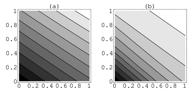
Figure 1: (a) The contour plots of $Y=Y(X)$ for the mass squared of the lowest bound state in units of $g^{2}N/\pi$ as a function of $X=m\pi/g^{2}N$ and Y (b)The contour plots of $Y=Y(X)$ for the mass squared of the second lowest bound state in units of $g^{2}N/\pi$ as a function of $X=m\pi/g^{2}N$ and Y (b)

In Fig. 1 we show the contour plots of the mass squared $M^{2}$ of the two lightest bosonic bound states as a function of $X$ and $Y$ at resolution $K=10$. These contours are lines of constant mass squared. Selecting a particular value of the mass of the first bound state then fixes a particular contour in Fig. 1a as a contour of fixed mass, which we can write as $Y=Y_{p}(X)$.

Interestingly, constructing the same contour plot for the next to lightest bosonic bound state – see Fig. 1b – yields contours that have approximately the same functional dependence implied by Fig. 1a. In fact, one obtains approximately the same contour plots for the next twenty bound states (which is as far as we checked). The simple conclusion is that the coupling $Y$ which represents the strength of the additional operator affects all bound state masses more or less equally. This in turn suggests that at finite resolution, we can smoothly interpolate between different values of fermion mass $X$, and different prescriptions specified by the coupling $Y$, without affecting too much the actual numerical spectrum. Of course, in the decompactification limit $K\rightarrow\infty$, such a dependence on $Y$ disappears, due to scheme independence.

Since the lightest bosonic bound state is primarily a two particle state it is reasonable to truncate the Fock basis to two particle states. This will permit very high resolutions, which will be needed to carefully scrutinize any possible discrepancies between the two versions of ’soft’ symmetry breaking presented here. In fact, we are able to study the theory for $K$ up to 800. The mass of the lowest state as a function of the resolution for various values of $X$ and $Y$ are shown in Fig. 2. Each converging pair of lines – which extrapolate the actual data points – in Fig. 2 corresponds to different values of fermion mass $X$. The top upper curve in each pair runs through data points that were calculated via SDLCQ (i.e. $Y=1$), while the lower corresponds to the PV (i.e. $Y=0$) prescription commonly adopted in the literature. We find that each pair of curves converge to the same point at infinite resolution, although this may not be completely obvious for the lowest pair in the figure (corresponding to the critical mass $X=0$).

Away from $X=0$, the SDLCQ formulation is fitted with a linear function of $1/K$, while the PV formulation is fit with a polynomial of $1/K^{2\beta}$, where $\beta$ is the solution of $1-X/2=\pi\beta Cot(\pi\beta)$ [79]. It now appears that SDLCQ not only provides more rapid convergence for supersymmetric models, but also for the massive t’Hooft model, which is not supersymmetric. For the massless case, the situation is reversed; the SDLCQ formulation converges slower. It is fit by a polynomial in $1/Log(K)$ and gives the same mass at infinite resolution as the PV formulation. This behavior may be understood from the observation that the wave function of this state does not vanish at $x=0$. We have looked closely at ‘small’ masses, such as $X=.1$, and one finds that both PV and SDLCQ vary as a polynomial in $1/K^{2\beta}$ at large resolution. Thus careful extrapolation schemes must be adopted at small masses.

We therefore conclude that the continuum of regularization schemes that interpolate smoothly between the SDLCQ and PV prescriptions – which we characterized by the parameter $Y$ – yield the same continuum bound state masses, although the rate of convergence of the DLCQ spectrum may be altered significantly. This implies that the contour plots observed in Fig. 1 eventually approach lines parallel to the $Y$ axis, and the sole dependence on the parameter $X$ is recovered.

Figure 2: Mass of the of the lowest bound state in units of $g^{2}N/\pi$ calculated in the t’Hooft model. The top pair is at $X=1$, the second is at $X=.5$, and the bottom pair is at $X=0$

Interestingly, since the two-body equation studied here for the adjoint fermion model is simply the t’Hooft equation with a rescaling of coupling constant, we have arrived at an alternative prescription for regulating the Coulomb singularity in the massive t’Hooft model that improves the rate of convergence towards the actual continuum mass. Thus, a prescription that arises naturally in the study of supersymmetric theories is also applicable in the study of a theory without supersymmetry. We believe that this idea deserves to be exploited further in a wider context of theories. In particular, it is an open question whether this procedure could provide a sensible approach to regularizing softly broken gauge theories with bosonic degrees of freedom, and in higher dimensions.

In any case, it appears that the special cancellations afforded by supersymmetry – especially in the context of DLCQ bound state calculations – might have scope beyond the domain of supersymmetric field theory. This would be a crucial first step towards a serious non-perturbative study of theories with broken supersymmetry.

4 Massless States in Two Dimensional Models.

In this section we will study the structure of bound states for two dimensional supersymmetric models defined in section 1. We will concentrate most of the attention on the model obtained by dimensional reduction from SYM₂₊₁. For this theory we will prove that any normalizable bound state in the continuum must include a contribution with arbitrarily large number of partons. By generalizing this proof to the theories with extended SUSY we show that this is the general property of supersymmetric matrix models. This scenario is to be contrasted with the simple bound states discovered in a number of $1+1$ dimensional theories with complex fermions, such as the Schwinger model, the t’Hooft model, and a dimensionally reduced theory with complex adjoint fermions [12, 69]. We also study the massless states of SYM₂₊₁ in DLCQ. Some of them are constructed explicitly and the general formula for the number of massless states as function of harmonic resolution is derived for the large $N$ case. This section is based in part on the results of [5].

4.1 Formulation of the bound state problem.

The light-cone formulation of the supersymmetric matrix model obtained by dimensionally reducing ${\cal N}=1$ $\mbox{SYM}_{2+1}$ to $1+1$ dimensions was initially given in [64], and it was summarized in the section 2 of these lectures. We simply note here that the light-cone Hamiltonian $P^{-}$ is given in terms of the supercharge $Q^{-}$ via the supersymmetry relation $\{Q^{-},Q^{-}\}=2\sqrt{2}P^{-}$, where

$$Q^{-}=2^{3/4}g\int dx^{-}\mbox{tr}\left\{({\rm i}[\phi,\partial_{-}\phi]+2\psi\psi)\frac{1}{\partial_{-}}\psi\right\}.$$ (4.1)

In the above, $\phi_{ij}=\phi_{ij}(x^{+},x^{-})$ and $\psi_{ij}=\psi_{ij}(x^{+},x^{-})$ are $N\times N$ Hermitian matrix fields representing the physical boson and fermion degrees of freedom (respectively) of the theory, and are remnants of the physical transverse degrees of freedom of the original $2+1$ dimensional theory. This is a special feature of light-cone quantization in light-cone gauge: all unphysical degrees of freedom present in the original Lagrangian may be explicitly eliminated. There are no ghosts.

In order to quantize $\phi$ and $\psi$ on the light-cone, we first introduce the following expansions at fixed light-cone time $x^{+}=0$ (the continuum counterpart of (2.2):

$$\phi_{ij}(x^{-},0)=\frac{1}{\sqrt{2\pi}}\int_{0}^{\infty}\frac{dk^{+}}{\sqrt{2k^{+}}}\left(a_{ij}(k^{+})e^{-ik^{+}x^{-}}+a^{\dagger}_{ji}(k^{+})e^{ik^{+}x^{-}}\right);$$ (4.2)

$$\psi_{ij}(x^{-},0)=\frac{1}{2\sqrt{\pi}}\int_{0}^{\infty}dk^{+}\left(b_{ij}(k^{+})e^{-ik^{+}x^{-}}+b^{\dagger}_{ji}(k^{+})e^{ik^{+}x^{-}}\right).$$ (4.3)

We then specify the commutation relations

$$\left[a_{ij}(p^{+}),a^{\dagger}_{lk}(q^{+})\right]=\left\{b_{ij}(p^{+}),b^{\dagger}_{lk}(q^{+})\right\}=\delta(p^{+}-q^{+})\delta_{il}\delta_{jk}$$ (4.4)

for the gauge group U($N$), or

$$\left[a_{ij}(p^{+}),a^{\dagger}_{lk}(q^{+})\right]=\left\{b_{ij}(p^{+}),b^{\dagger}_{lk}(q^{+})\right\}=\delta(p^{+}-q^{+})\left(\delta_{il}\delta_{jk}-\frac{1}{N}\delta_{ij}\delta_{kl}\right)$$ (4.5)

for the gauge group SU($N$).

For the bound state eigen-problem $2P^{+}P^{-}|\Psi>=M^{2}|\Psi>$, we may restrict to the subspace of states with fixed light-cone momentum $P^{+}$, on which $P^{+}$ is diagonal, and so the bound state problem is reduced to the diagonalization of the light-cone Hamiltonian $P^{-}$. Since $P^{-}$ is proportional to the square of the supercharge $Q^{-}$, any eigenstate $|\Psi>$ of $P^{-}$ with mass squared $M^{2}$ gives rise to a natural four-fold degeneracy in the spectrum because of the supersymmetry algebra—all four states below have the same mass:

$$|\Psi>,\hskip 11.38109ptQ^{+}|\Psi>,\hskip 11.38109ptQ^{-}|\Psi>,\hskip 11.38109ptQ^{+}Q^{-}|\Psi>.$$ (4.6)

Although this four-fold degeneracy is realized in the continuum formulation of the theory, this property will not necessarily survive if we choose to discretize the theory in an arbitrary manner. However, a nice feature of SDLCQ is that it does preserve the supersymmetry (and hence the exact four-fold degeneracy) for any resolution.

Focusing attention on zero mass eigenstates, we simply note that a massless eigenstate of $P^{-}$ must also be annihilated by the supercharge $Q^{-}$, since $P^{-}$ is proportional to $(Q^{-})^{2}$. Thus the relevant eigen-equation is $Q^{-}|\Psi>=0$. We wish to study this equation. However, first we need to state the explicit equation for $Q^{-}$, in the momentum representation, which is obtained by substituting the quantized field expressions (4.2) and (4.3) directly into the the definition of the supercharge (4.1). The result is:

$$Q^{-} = {{\rm i}2^{-1/4}g\over\sqrt{\pi}}\int_{0}^{\infty}dk_{1}dk_{2}dk_{3}\delta(k_{1}+k_{2}-k_{3})\left\{\frac{}{}\right.$$

$${1\over 2\sqrt{k_{1}k_{2}}}{k_{2}-k_{1}\over k_{3}}[a_{ik}^{\dagger}(k_{1})a_{kj}^{\dagger}(k_{2})b_{ij}(k_{3})-b_{ij}^{\dagger}(k_{3})a_{ik}(k_{1})a_{kj}(k_{2})]$$

$${1\over 2\sqrt{k_{1}k_{3}}}{k_{1}+k_{3}\over k_{2}}[a_{ik}^{\dagger}(k_{3})a_{kj}(k_{1})b_{ij}(k_{2})-a_{ik}^{\dagger}(k_{1})b_{kj}^{\dagger}(k_{2})a_{ij}(k_{3})]$$

$${1\over 2\sqrt{k_{2}k_{3}}}{k_{2}+k_{3}\over k_{1}}[b_{ik}^{\dagger}(k_{1})a_{kj}^{\dagger}(k_{2})a_{ij}(k_{3})-a_{ij}^{\dagger}(k_{3})b_{ik}(k_{1})a_{kj}(k_{2})]$$

$$({1\over k_{1}}+{1\over k_{2}}-{1\over k_{3}})[b_{ik}^{\dagger}(k_{1})b_{kj}^{\dagger}(k_{2})b_{ij}(k_{3})+b_{ij}^{\dagger}(k_{3})b_{ik}(k_{1})b_{kj}(k_{2})]\left.\frac{}{}\right\}.$$

(4.7)

In order to implement the DLCQ formulation [68, 63] of the theory, we simply restrict the momenta $k_{1},k_{2}$ and $k_{3}$ appearing in the above equation to the following set of allowed momenta: $\{\frac{P^{+}}{K},\frac{2P^{+}}{K},\frac{3P^{+}}{K},\dots\}$. Here, $K$ is some arbitrary positive integer, and must be sent to infinity if we wish to recover the continuum formulation of the theory. The integer $K$ is called the harmonic resolution, and $1/K$ measures the coarseness of our discretization. Physically, $1/K$ represents the smallest unit of longitudinal momentum fraction allowed for each parton. As soon as we implement the DLCQ procedure, which is specified unambiguously by the harmonic resolution $K$, the integrals appearing in the definition of $Q^{-}$ are replaced by finite sums, and the eigen-equation $Q^{-}|\Psi>=0$ is reduced to a finite matrix problem. For sufficiently small values of $K$ (in this case for $K\leq 4$) this eigen-problem may be solved analytically. For values $K>5$, we may still compute the DLCQ supercharge analytically as a function of $N$, but the diagonalization procedure must be performed numerically.

For now, we concentrate on the structure of the zero mass eigenstates for the continuum theory. Firstly, note that for the U($N$) bound state problem, massless states appear automatically because of the decoupling of the U($1$) and SU($N$) degrees of freedom that constitute U($N$). More explicitly, we may introduce the U(1) operators

$$\alpha(k^{+})=\frac{1}{N}\mbox{tr}[a(k^{+})]\hskip 11.38109pt\mbox{and}\hskip 11.38109pt\beta(k^{+})=\frac{1}{N}\mbox{tr}[b(k^{+})],$$ (4.8)

which allow us to decompose any U($N$) operator into a sum of U(1) and SU($N$) operators:

$$a(k^{+})=\alpha(k^{+})\cdot\mbox{${\bf 1}_{N\times N}$}+{\tilde{a}}(k^{+})\hskip 11.38109pt\mbox{and}\hskip 11.38109ptb(k^{+})=\beta(k^{+})\cdot\mbox{${\bf 1}_{N\times N}$}+{\tilde{b}}(k^{+}),$$ (4.9)

where ${\tilde{a}}(k^{+})$ and ${\tilde{b}}(k^{+})$ are traceless $N\times N$ matrices. If we now substitute the operators above into the expression for the supercharge (4.1), we find that all terms involving the U(1) factors $\alpha(k^{+}),\beta(k^{+})$ vanish – only the SU($N$) operators ${\tilde{a}}(k^{+}),{\tilde{b}}(k^{+})$ survive. i.e. starting with the definition of the U($N$) supercharge, we end up with the definition of the SU($N$) supercharge. In addition, the (anti)commutation relations $[{\tilde{a}}_{ij}(k_{1}),\alpha^{\dagger}(k_{2})]=0$ and $\{{\tilde{b}}_{ij}(k_{1}),\beta^{\dagger}(k_{2})\}=0$ imply that this supercharge acts only on the SU($N$) creation operators of a fock state - the U(1) creation operators only introduce degeneracies in the SU($N$) spectrum. Clearly, since $Q^{-}$ has no U(1) contribution, any fock state made up of only U(1) creation operators must have zero mass. The non-trivial problem here is to determine whether there are massless states for the SU($N$) sector. We will address this topic next.

4.2 The Proof for (1,1) Model.

It was pointed out in the previous subsection that a zero mass eigenstate is annihilated by the light-cone supercharge (4.1):

$$Q^{-}|\Psi\rangle=0$$ (4.10)

We wish to show that if such an SU($N$) eigenstate is normalizable, then it must involve a superposition of an infinite number of Fock states. The basic strategy is quite simple: normalizability will impose certain conditions on the light-cone wave functions as one or several momentum variables vanish. Moreover, if we assume a given eigenstate $|\Psi\rangle$ has at most $n$ partons, then the terms in $Q^{-}|\Psi\rangle$ consisting of $n+1$ partons must sum to zero, providing relations between the $n$ parton wave functions only. We then show these wave functions must all vanish by studying various zero momentum limits of these relations. Interestingly, the utility of studying light-cone wave functions at small momenta also appears in the context of light-front $\mbox{QCD}_{3+1}$ [3].

In order to proceed with a systematic presentation of the proof, we start by considering the large $N$ limit case. This simply means that we consider Fock states that are made from a single trace of a product of boson or fermion creation operators acting on the light-cone Fock vacuum $|0\rangle$. Multiple trace states correspond to $1/N$ corrections to the theory, and are therefore ignored. In this limit, a general state $|\Psi\rangle$ is a superposition of Fock states of any length, and may be written in the form

$$|\Psi\rangle=\sum_{n=2}^{\infty}\sum_{r=0}^{n}\sum_{P}\int_{0}^{P^{+}}{dq_{1}\dots dq_{n}\over\sqrt{q_{1}...q_{n}}}\delta(q_{1}+\cdots+q_{n}-P^{+})\times$$ (4.11)

$$\hskip 71.13188ptf^{(n,r)}_{P}(q_{1},\dots,q_{n})\mbox{tr}[c^{\dagger}(q_{1})\dots c^{\dagger}(q_{n})]|0\rangle,$$

where $c^{\dagger}(q^{+})$ represents either a boson or fermion creation operator carrying light-cone momentum $q^{+}$, and $f^{(n,r)}_{P}$ denotes the wave function of an $n$ parton Fock state containing $r$ fermions in a particular arrangement $P$. It is implied that we sum over all such arrangements, which may not necessarily be distinct with respect to cyclic symmetry of the trace.

At this point, we simply remark that normalizability of a general state $|\Psi\rangle$ above implies

$$\int_{0}^{P^{+}}{dq_{1}\dots dq_{n}\over q_{1}\dots q_{n}}\delta(q_{1}+\cdots+q_{n}-P^{+})|f^{(n,r)}_{P}(q_{1},\dots,q_{n})|^{2}<\infty$$ (4.12)

for any particular wave function $f^{(n,r)}_{P}$. Therefore, any wave function vanishes if one or several of its momenta are made to vanish.

We are now ready to carry out the details of the proof. But first a little notation. We will write $|\Psi_{(n,m)}\rangle$ to denote a superposition of all Fock states – as in (4.11) – with precisely $n$ partons, $m$ of which are fermions. Such a Fock expansion involves only the wave functions $f^{(n,m)}_{P}$, and the number of them is enumerated by the index $P$. For the special case $|\Psi_{(n,0)}\rangle$ (i.e. no fermions), there is only one wave function, which we denote by $f^{(n,0)}$ for brevity:

$$|\Psi_{(n,0)}\rangle=\int_{0}^{P^{+}}{dq_{1}\dots dq_{n}\over\sqrt{q_{1}...q_{n}}}\delta(q_{1}+...+q_{n}-P^{+})\hskip 2.84526ptf^{(n,0)}(q_{1}...q_{n})\mbox{tr}[a^{\dagger}(q_{1})...a^{\dagger}(q_{n})]|0\rangle.$$ (4.13)

There is another special case we wish to consider; namely, the state $|\Psi_{(n,2)}\rangle$ consisting of $n$ parton Fock states with precisely two fermions. If we place one of the fermions at the beginning of the trace, then there are $n-1$ ways of positioning the second fermion, yielding $n-1$ possible wave functions. We will enumerate such wave functions by the subscript index $k$, as in $f^{(n,2)}_{k}$, where $k=2,3,\dots,n$. The subscript $k$ denotes the location of the second fermion. Explicitly, we have

$$|\Psi_{(n,2)}\rangle=\sum_{k=2}^{n}\int_{0}^{P^{+}}{dq_{1}\dots dq_{n}\over\sqrt{q_{1}...q_{n}}}\delta(q_{1}+\cdots+q_{n}-P^{+})\times$$

$$\hskip 42.67912ptf^{(n,2)}_{k}(q_{1},\dots,q_{k},\dots,q_{n})\mbox{tr}[b^{\dagger}(q_{1})a^{\dagger}(q_{2})\dots b^{\dagger}(q_{k})\dots a^{\dagger}(q_{n})]|0\rangle.$$

(4.14)

Of course, depending upon the symmetry, the $n-1$ Fock states enumerated in this way need not be distinct with respect to the cyclic properties of the trace. This provides us with additional relations between wave functions – a fact we will make use of later on.

Now let us assume that $|\Psi\rangle$ is a normalizable SU($N$) zero mass eigenstate with at most $n$ partons. Glancing at the form of (4.1), we see that the $n+1$ parton Fock states containing a single fermion in each of the combinations $Q^{-}|\Psi_{(n,0)}\rangle$ and $Q^{-}|\Psi_{(n,2)}\rangle$ must cancel each other to guarantee a massless eigenstate. This immediately gives rise to the following wave function relation:

$$\frac{q_{1}+2q_{2}}{q_{1}+q_{2}}f^{(n,0)}(q_{1}+q_{2},q_{3},\dots,q_{n+1})-\frac{q_{1}+2q_{n+1}}{q_{1}+q_{n+1}}f^{(n,0)}(q_{n+1}+q_{1},q_{2},\dots,q_{n})=$$

$$=2\frac{\sqrt{q_{1}}}{n}\sum_{k=2}^{n}\frac{q_{k+1}-q_{k}}{(q_{k+1}+q_{k})^{3/2}}f^{(n,2)}_{k}(q_{1},\dots,q_{k-1},q_{k}+q_{k+1},q_{k+2},\dots,q_{n+1}).$$

(4.15)

In the limit $q_{i}\rightarrow 0$, for $3\leq i\leq n$, this last equation is reduced to

$$\frac{1}{\sqrt{q_{i+1}}}f^{(n,2)}_{i}(q_{1},\dots,q_{i-1},q_{i+1},\dots,q_{n+1})$$ (4.16)

$$\hskip 71.13188pt-\frac{1}{\sqrt{q_{i-1}}}f^{(n,2)}_{i-1}(q_{1},\dots,q_{i-1},q_{i+1},\dots,q_{n+1})=0.$$

An immediate consequence is that any wave function $f^{(n,2)}_{i}$ for $i=3,4,\dots,n$, may be expressed in terms of $f^{(n,2)}_{2}$. Explicitly, we have

$$f^{(n,2)}_{i}(q_{1},q_{2},\dots,q_{n})=\sqrt{\frac{q_{i}}{q_{2}}}f^{(n,2)}_{2}(q_{1},q_{2},\dots,q_{n}),\hskip 22.76219pti=3,4,\dots,n.$$ (4.17)

Moreover, the limit $q_{2}\rightarrow 0$ of equation (4.2) yields the further relation after a suitable change of variables:

$$f^{(n,0)}(q_{1},q_{2},q_{3},\dots,q_{n}) = \frac{2}{n}\sqrt{\frac{q_{1}}{q_{2}}}f^{(n,2)}_{2}(q_{1},q_{2},q_{3},\dots,q_{n}).$$ (4.18)

Finally, because of the cyclic properties of the trace, there is an additional relation between wave functions:

$$f^{(n,2)}_{i}(q_{1},q_{2},\dots,q_{i},\dots,q_{n})=-f^{(n,2)}_{n-i+2}(q_{i},q_{i+1},\dots,q_{n},q_{1},q_{2},\dots,q_{i-1}).$$ (4.19)

Setting $i=2$ in the above equation, and $i=n$ in equation (4.17), we deduce

$$f^{(n,2)}_{2}(q_{1},q_{2},\dots,q_{n})=-\sqrt{\frac{q_{1}}{q_{2}}}f^{(n,2)}_{2}(q_{2},q_{3},\dots,q_{n},q_{1}).$$ (4.20)

Combining this with equation (4.18), we conclude $(\frac{\sqrt{q_{2}}}{q_{1}}+\frac{\sqrt{q_{3}}}{q_{2}})f^{(n,0)}(q_{1},\dots,q_{n})=0$, where we use the fact that the wave functions $f^{(n,0)}$ are cyclically symmetric. Thus $f^{(n,0)}$ must vanish. It immediately follows that $f^{(n,2)}_{i}$ vanish for all $i$ as well.

To summarize, we have shown that if $|\Psi\rangle$ is a normalizable zero mass eigenstate, where each Fock state in its Fock state expansion has no more than $n$ partons, the contributions $|\Psi_{(n,0)}\rangle$ and $|\Psi_{(n,2)}\rangle$ in this Fock state expansion must vanish. Since we may assume $|\Psi\rangle$ is bosonic, the only other contributions involve Fock states with an even number of fermions: $|\Psi_{(n,4)}\rangle$, $|\Psi_{(n,6)}\rangle$, and so on. We claim that all such contributions vanish. To see this, first observe that the $n+1$ parton Fock states with three fermions in the combinations $Q^{-}|\Psi_{(n,2)}\rangle$ and $Q^{-}|\Psi_{(n,4)}\rangle$ must cancel each other, in order to guarantee a zero eigenstate mass. But our previous analysis demonstrated that $|\Psi_{(n,2)}\rangle\equiv 0$, and thus the $n+1$ parton Fock states with three fermions in $Q^{-}|\Psi_{(n,4)}\rangle$ alone must sum to zero.

We are now ready to perform an induction procedure. Namely, we assume that for some positive integer $k$ the state $|\Psi_{(n,2[k-1])}\rangle$ vanishes. Then the $n+1$ parton Fock states in $Q^{-}|\Psi\rangle$ which contain $2k-1$ fermions receive contributions only from $Q^{-}|\Psi_{(n,2k)}\rangle$ in which a fermion is replaced by two bosons. This has to sum to zero. We therefore obtain a relation among the wave functions $f^{(n,2k)}_{P}$ by considering the action of the supercharge (4.1) in which a fermion is replaced by two bosons. Keeping in mind that we are free to renormalize any wave function by a constant, we end up with the following relation:

$$\sum_{P}{f}^{(n,2k)}_{P}(s_{1},\dots,s_{i-1},s_{i}+s_{i+1},s_{i+2},\dots,s_{n+1})\frac{s_{i+1}-s_{i}}{(s_{i+1}+s_{i})^{3/2}}=0.$$ (4.21)

It is now an easy task to show that the wave functions ${f}^{(n,2k)}_{P}$ appearing in equation (4.21) must vanish; one simply considers various limits $s_{j}\rightarrow 0$ as we did before. This completes our proof by induction. Namely, there can be no non-trivial normalizable massless state with an upper limit on the number of allowed partons. Of course, this proof is valid only in the large $N$ limit. We now turn our attention to the finite $N$ case.

Let us define $Q^{-}_{lead}$ to be that part of the supercharge $Q^{-}$ that replaces a fermion with two bosons, or replaces a boson with a boson and fermion pair. As in the large $N$ case we begin by assuming that we have a normalizable zero mass eigenstate $|\Psi\rangle$ which is a sum of Fock states that have at most $n$ partons. The proof for finite $N$ consists of two parts. First, we consider bosonic states consisting of only $n$ parton Fock states that have at most two fermions, and show the wave functions must vanish. We then invoke an induction argument to consider $n$ parton wave functions involving an even number of fermions, and show they must vanish as well.

The additional complication introduced by the assumption that $N$ is finite is that a given Fock state may involve more than just a single trace. However, note that $Q^{-}_{lead}$ cannot decrease the number of traces; it can either increase the number of traces by one, or leave the number unchanged. Thus we have a natural induction procedure in the number of traces as well. Since the terms in $Q^{-}_{lead}$ have only one annihilation operator, it acts on a given product of traces according to the Leibniz rule:

$$Q^{-}_{lead}\left(\mbox{tr}[A]\mbox{tr}[B]\dots\right)|0\rangle=\left(Q^{-}_{lead}\mbox{tr}[A]\right)\mbox{tr}[B]\dots|0\rangle+$$

$$(-1)^{F(A)}\mbox{tr}[A]Q^{-}_{lead}\left(\mbox{tr}[B]\dots\right)|0\rangle.$$ (4.22)

Schematically, the general structure of an arbitrary Fock state with $k$ traces has the form

$$f^{(n,i_{1},i_{2},\dots,i_{k})}_{P}\mbox{tr}[(b^{\dagger})^{i_{1}}a^{\dagger}\dots a^{\dagger}]\dots\mbox{tr}[(b^{\dagger})^{i_{k}}a^{\dagger}\dots a^{\dagger}]|0\rangle,$$ (4.23)

where $n$ denotes the total number of partons in each Fock state, and the integers $i_{1},i_{2},\dots$ denote the number of fermions in the first trace, second trace, and so on. We will always order the traces so that the number of fermions in each trace decreases to the right. The index $P$ labels a particular arrangement of fermions.

We now consider the $n+1$ parton Fock states of $Q^{-}_{lead}|\Psi\rangle$ that have precisely one fermion. The only possible contributions involve three types of wave functions; $f^{(n,0)}$, $f^{(n,2)}_{P}$ and $f^{(n,1,1)}$ (we only include the permutation index $P$ if there is more than one distinct arrangement). If these three wave functions contribute to the same one fermion Fock state, then the distribution of bosons in the Fock state corresponding to $f^{(n,2)}_{P}$ determines the distribution of bosons for $f^{(n,0)}$ and $f^{(n,1,1)}$. We allow $Q^{-}_{lead}$ to act only on the first trace in both $f^{(n,0)}$ and $f^{(n,2)}_{P}$, and only on the second one in $f^{(n,1,1)}$. If there are more than two traces in these states they must be identical in all the components, and so don’t play a role in the calculation. Thus, it is sufficient to consider states with two traces only. Such a state has the form

$$|\Phi>=\int_{0}^{P^{+}}{d^{m+n}q\over\sqrt{q_{1}\dots q_{n+m}}}\delta(q_{1}+\cdots+q_{n+m}-P^{+})$$ (4.24)

$$f^{(n+m,0)}(q_{1},\dots,q_{m}|q_{m+1},\dots,q_{m+n})$$

$$\times\mbox{tr}\left[a^{\dagger}(q_{1})\dots a^{\dagger}(q_{m})\right]\mbox{tr}\left[a^{\dagger}(q_{m+1})\dots a^{\dagger}(q_{m+n})\right]|0\rangle$$

$$+\int_{0}^{P^{+}}{d^{m+n-2}qdp_{1}dp_{2}\over\sqrt{q_{1}\dots q_{n+m-2}p_{1}p_{2}}}\delta(q_{1}+\cdots+q_{n+m-2}+p_{1}+p_{2}-P^{+})\left\{\frac{}{}\right.$$

$$f^{(n+m,1,1)}(p_{1},q_{1},\dots,q_{m}|p_{2},q_{m+3},\dots,q_{m+n})\times$$

$$\times\mbox{tr}\left[b^{\dagger}(p_{1})a^{\dagger}(q_{1})\dots a^{\dagger}(q_{m})]\mbox{tr}[b^{\dagger}(p_{2})a^{\dagger}(q_{m+3})\dots a^{\dagger}(q_{m+n})\right]+$$

$$+\sum_{P}f^{(n+m,2)}_{P}(p_{1},P[q_{1}\dots q_{m-2};p_{2}]|q_{m+1}\dots q_{m+n})\times$$

$$\left.\times\mbox{tr}\left(b^{\dagger}(p_{1})P[a^{\dagger}(q_{1})\dots a^{\dagger}(q_{m-2});b^{\dagger}(p_{2})]\right)\mbox{tr}\left[a^{\dagger}(q_{m+1})\dots a^{\dagger}(q_{m+n})\right]\frac{}{}\right\}|0\rangle,$$

where we have summed over the index $P$ representing all possible permutation arrangements of bosons and fermions that contribute. We then find:

$${F}(p,q_{1},\dots,q_{m}|q_{m+1},q_{m+2},\dots,q_{m+n})+$$

$$+\frac{q_{m+2}-q_{m+1}}{(q_{m+2}+q_{m+1})^{3/2}}{f}^{(n+m,1,1)}(p,q_{1}\dots q_{m}|q_{m+1}+q_{m+2},q_{m+3}\dots q_{m+n})=0,$$

where $F$ is the contribution from $f^{(n+m,0)}$ and $f^{(n+m,2)}_{P}$. Now we see that the limit $q_{m+1}\rightarrow 0$ gives: $f^{(n+m,1,1)}\equiv 0$. Thus if (4.24) represents a contribution to the massless eigenstate state $|\Psi\rangle$, then $|\Phi\rangle$ takes the form

$$|\Phi\rangle = \int_{0}^{P^{+}}{d^{m+n-2}qdK^{+}\over\sqrt{q_{1}\dots q_{n+m-2}}}\delta(q_{1}+\cdots+q_{n+m-2}-(P^{+}-K^{+}))\left[\frac{}{}\right.$$

$$\int_{0}^{P^{+}}{dq_{m-1}dq_{m}\over\sqrt{q_{m-1}q_{m}}}\delta(q_{m-1}+q_{m}-K^{+})$$

$$f^{(n+m,0)}(q_{1},\dots,q_{m}|q_{m+1},\dots,q_{m+n})\mbox{tr}(a^{\dagger}(q_{1})\dots a^{\dagger}(q_{m}))$$

$$+ \int_{0}^{P^{+}}{dp_{1}dp_{1}\over\sqrt{p_{1}p_{2}}}\delta(p_{1}+p_{2}-K^{+})$$

$$\sum_{P}f^{(n+m,2)}_{P}(p_{1},P[q_{1},\dots,q_{m-2};p_{2}]|q_{m+1},\dots,q_{m+n})$$

$$\left.\mbox{tr}(b^{\dagger}(p_{1})P[a^{\dagger}(q_{1})\dots a^{\dagger}(q_{m-2});b^{\dagger}(p_{2})])\mbox{tr}(a^{\dagger}(q_{m+1})\dots a^{\dagger}(q_{m+n}))\right]|0\rangle$$

and $Q^{-}_{lead}$ acts only on the terms in the square brackets. All these terms have only one trace, which is a scenario we already encountered in the large $N$ limit case. Using the results of that discussion, we find that the only massless solution of the form (4.2) is the trivial one. This is the starting point of the induction procedure for finite $N$.

As explained earlier, we look for $n$ parton Fock states in the expansion for $|\Psi\rangle$ that have $2k$ fermions ($k>1$), To finish the proof we need to show that for any $k$ the only allowed wave function is the trivial one. ¿From the large $N$ result we know there are no such one trace states. We now consider the state with an arbitrary number of traces,

$$|\Psi_{(n,2k)}\rangle=\sum_{P}\int_{0}^{P^{+}}{ds_{1}\dots ds_{n}\over\sqrt{s_{1}\dots s_{n}}}\delta(s_{1}+\cdots+s_{n}-P^{+})$$ (4.27)

$$f^{(n,2k)}_{P}(s_{1}\dots s_{i_{1}}|\dots|\dots s_{n})\mbox{tr}\left(c^{\dagger}(s_{1})\dots c^{\dagger}(s_{i_{1}})\right)\mbox{tr}\left(\dots\right)\mbox{tr}\left(\dots c^{\dagger}(s_{n})\right)|0\rangle,$$

then the analog of (4.21) for such states reads:

$${\sum_{i}}^{\prime}f^{(n,2k)}_{P_{i}}(s_{1}\dots|s_{j_{a}}\dots s_{i-1},s_{i}+s_{i+1},s_{i+2}\dots s_{j_{a}+k_{a}}|\dots s_{n+1})\frac{s_{i+1}-s_{i}}{(s_{i+1}+s_{i})^{3/2}}=0.$$ (4.28)

Here, $\sum_{i}^{\prime}$ means that for each trace we should include one additional term with $"i"=j_{a}+k_{a}$, $"i+1"=j_{a}$ if $c$ corresponding to both $j_{a}+k_{a}$ and $j_{a}$ is $a$. If the number of traces is $a$, we introduce

$$j_{a}=\sum_{b=1}^{a-1}k_{b}.$$

If any of the blocks $\mbox{tr}(\dots)$ in the state for which (4.28) is written contains two or more fermions, then, as in the large $N$ case, all the corresponding wave functions $f^{(n,2k)}_{P}$ vanish. So we only need to consider the states of the form:

$$|\Psi_{(n,k_{1}+1,\dots)}\rangle=\sum_{P}\int dpdqf^{(n,k_{1}+1,\dots)}_{P}(p_{1},q_{1},\dots,q_{k_{1}}|p_{2},q_{k_{1}+1},\dots,q_{k_{1}+k_{2}}|\dots)\times$$

$$\mbox{tr}\left(b^{\dagger}(p_{1})a^{\dagger}(q_{1})\dots a^{\dagger}(q_{k_{1}})\right)\mbox{tr}\left(b^{\dagger}(p_{2})a^{\dagger}(q_{k_{1}+1})\dots a^{\dagger}(q_{k_{1}+k_{2}})\right)\dots|0\rangle.$$

(4.29)

Let ${\tilde{Q}}$ denote that part of the supercharge $Q^{-}$ which replaces a fermion with two bosons. Let us consider the result of such a change in the first trace. Suppose there are $a$ traces having the same form as the first trace. Then without loss of generality, we may assume they are the first $a$ traces. Then using the symmetries of the wave functions we find:

$${\tilde{Q}}|\Psi_{(n,k_{1}+1,\dots)}\rangle=-\frac{1}{2\sqrt{2\pi}}\sum_{P}\int_{0}^{P^{+}}dkdpdq$$

$$f^{(n,k_{1}+1,\dots)}_{P}(p_{1},q_{1},\dots,q_{k_{1}}|p_{2},q_{k_{1}+1},\dots,q_{2k_{1}}|\dots)\sum_{b=1}^{a}\frac{p_{b}-2k}{p_{b}}\frac{1}{\sqrt{k(p_{b}-k)}}(-1)^{b+1}\times$$

$$\mbox{tr}\left(b^{\dagger}(p_{1})a^{\dagger}(q_{1})\dots a^{\dagger}(q_{k_{1}})\right)\dots\mbox{tr}\left(a^{\dagger}(k)a^{\dagger}(p_{b}-k)a^{\dagger}(q_{(b-1)k_{1}+1})\dots a^{\dagger}(q_{bk_{1}})\right)\dots|0\rangle$$

$$=-\frac{1}{2\sqrt{2\pi}}\sum_{P}\int_{0}^{P^{+}}dkdpdq\frac{p_{1}-2k}{p_{1}}\frac{1}{\sqrt{k(p_{1}-k)}}\mbox{tr}\left(a^{\dagger}(k)a^{\dagger}(p_{1}-k)a^{\dagger}(q_{1})\dots a^{\dagger}(q_{k_{1}})\right)\times$$

$$\mbox{tr}\left(b^{\dagger}(p_{2})a^{\dagger}(q_{k_{1}+1})\dots a^{\dagger}(q_{k_{1}+k_{2}})\right)\dots|0\rangle\sum_{b=1}^{a}(-1)^{b+1}(-1)^{b+1}\times$$

$$\hskip 28.45274ptf_{P}^{(n,k_{1}+1,\dots)}(p_{1},q_{1},\dots,q_{k_{1}}|p_{2},q_{k_{1}+1},\dots,q_{k_{1}+k_{2}}|\dots).$$

If the above expression vanishes then the only solution is the trivial one in which all wave functions vanish. This finishes the proof of the induction procedure for the finite $N$ case.

The extension of the proof to massive bound states is straightforward. Firstly, assume $|\Psi\rangle$ is a normalizable eigenstate of $2P^{+}P^{-}$ with mass squared $M^{2}\neq 0$. Then, since $P^{-}=\frac{1}{\sqrt{2}}(Q^{-})^{2}$, the state

$$|{\tilde{\Psi}}\rangle\equiv|\Psi\rangle+\alpha Q^{-}|\Psi\rangle$$ (4.30)

for $\alpha^{2}=\sqrt{2}P^{+}/M^{2}$ is a normalizable eigenstate of the supercharge $Q^{-}$, with eigenvalue $1/\alpha$. We therefore study the eigen-problem $Q^{-}|{\tilde{\Psi}}\rangle=\frac{1}{\alpha}|{\tilde{\Psi}}\rangle$. The resulting constraints on the wave functions may be obtained by modifying our original expressions by including a wave function multiplied by a finite constant. However, in our analysis, we always need to let some of the momenta vanish, and therefore this additional contribution vanishes. The analysis (and therefore the conclusions) remains unchanged.

We therefore conclude that any normalizable SU($N$) bound state (massless or massive) that exists in the model must be a superposition of an infinite number of Fock states.

4.3 Higher Dimensional Theories.

In this subsection we extend our theorem to the two–dimensional supersymmetric theories obtained as the result of dimensional reduction from $D>3$ dimensions. The most important cases are $D=4$, 6 and 10 which have $2$, $4$ and $8$ supersymmetries in two dimensions. Below we consider only large N case, the generalization to arbitrary $SU(N)$ group is trivial repetition of the arguments given in previous subsection.

Again our starting point is the fact that if there is normalizable eigenstate of Hamiltonian having finite length than its main symbol satisfies the condition:

$$Q^{-}_{lead}|\Psi>=0,$$ (4.31)

where $Q^{-}_{lead}$ is the part of supercharge increasing the number of partons. In three dimensional case we had only one supercharge $Q^{-}$, for general $D$ dimensional SYM reduced in $1+1$ there are $D-2$ supercharges, each of them squared gives $P^{-}$ and (4.31) should be true for all of them. In general different supercharges are not anticommute with each other, but since we consider quantization near trivial classical configuration (with no monopoles and no external charges) then they do. It is easy to derive the general form of supercharge:

$$Q^{-}_{\alpha} = \int_{o}^{\infty}\frac{dk}{k}(b^{\alpha\dagger}_{ij}(k)J_{ij}(-k)-(J_{ij}(-k))^{\dagger}b^{\alpha}_{ij}(k))+$$

$$+ \frac{\mu}{2\sqrt{2\pi}}\int_{-\infty}^{\infty}dkM^{\alpha\beta}_{IJ}[A_{I},A_{J}]_{ij}(k){\Psi}^{\beta}_{ji}(-k),$$

$$J_{ij}(-k) = \frac{1}{2\sqrt{2\pi}}\int_{o}^{\infty}dp\frac{2p+k}{\sqrt{p(p+k)}}\left(a^{I\dagger}_{ki}(p)a^{I}_{kj}(k+p)-a^{I\dagger}_{jk}(p)a^{I}_{ik}(k+p)\right)+$$

$$+ \frac{1}{2\sqrt{2\pi}}\int_{o}^{k}dp\frac{k-2p}{\sqrt{p(k-p)}}a^{I}_{ik}(p)a^{I}_{kj}(k-p)+\frac{1}{\sqrt{2\pi}}\int_{o}^{k}dpb^{\alpha}_{ik}(p)b^{\alpha}_{kj}(k-p)+$$

$$+ \frac{1}{\sqrt{2\pi}}\int_{o}^{\infty}dp\left(b^{\alpha\dagger}_{ki}(p)b^{\alpha}_{kj}(k+p)-b^{\alpha\dagger}_{jk}(p)b^{\alpha}_{ik}(k+p)\right).$$

In the above expression we introduced $d=D-2$ kinds of bosons ($I=1,...,d$) and $d$ kinds of fermions ($\alpha=1,...,d$) which we get as the result of compactification. The $\mu$ is nonzero constant depending on $D$ and $M$ are combinations of $d$ dimensional Dirac matrices:

$$M^{\alpha\beta}_{IJ}=(\gamma_{I}\gamma^{T}_{J}-\gamma_{J}\gamma^{T}_{I})_{\alpha\beta}.$$ (4.34)

As before our proof is based on the induction on the number of fermionic operators in the state. First we consider main symbol being superposition of purely bosonic states and ones containing two fermionic operators. Now we have $d$ types of bosons and $d$ types of fermions so some additional indices should be included in the wavefunctions. Defining bosonic indexes to be capital letters $A,\ B...$ and fermionic ones to be Greek letters we write:

$$|\Psi,0> = \int_{0}^{P^{+}}\frac{dq_{1}...dq_{n}}{\sqrt{q_{1}...q_{n}}}\delta(q_{1}+...+q_{n}-P^{+})\sum_{A}f^{(0)}_{[A_{1}...A_{n}]}(q_{1}...q_{n})\times$$ (4.35)

$$\times tr[a^{\dagger}_{A_{1}}(q_{1})...a^{\dagger}_{A_{n}}(q_{n})]|0>,$$

$$|\Psi,2> = \sum_{k=1}^{n-1}\int_{0}^{P^{+}}\frac{dq_{1}...dq_{n}}{\sqrt{q_{1}...q_{n}}}\delta(q_{1}+...+q_{n}-P^{+})\sum_{A,\alpha}f^{(2)k}_{[A_{1}...A_{k-1}\alpha_{1}A_{k}...A_{n-2}\alpha_{2}]}(q_{1}...q_{n})\times$$ (4.36)

$$\times tr[a^{\dagger}_{A_{1}}(q_{1})...a^{\dagger}_{A_{k-1}}(q_{k-1})b^{\dagger}_{\alpha_{1}}(q_{k})a^{\dagger}_{A_{k}}(q_{k+1})...a^{\dagger}_{A_{n-2}}(q_{n-1})b^{\dagger}_{\alpha_{2}}(q_{n})]|0>.$$

It is now easy to find the one fermionic part of the result of action by (4.3) on the main symbol of the state. The vanishing of this contribution leads to the generalization of the equation (4.2):

$$\delta_{\alpha\beta}\frac{n}{p}\left(\frac{2q_{n}+p}{q_{n}+p}f^{(0)}_{A_{1}...A_{n}}(q_{1}...q_{n-1},q_{n}+p)-\frac{2q_{1}+p}{q_{1}+p}f^{(0)}_{A_{1}...A_{n}}(q_{1}+p...q_{n-1},q_{n})\right)-$$

$$\frac{2}{\sqrt{p}}\sum_{k=1}^{n-1}\frac{q_{k+1}-q_{k}}{(q_{k+1}+q_{k})^{3/2}}\delta_{A_{k}A_{k+1}}f^{(2)k}_{[A_{1}...A_{k-1}\alpha A_{k+2}...A_{n}\beta]}(q_{1}...q_{k-1},q_{k}+q_{k+1},q_{k+2}...q_{n},p)+$$

$$n\mu\left(\frac{M^{\alpha\beta}_{A_{n}B}}{q_{n}+p}f^{(0)}_{A_{1}...A_{n-1}B}(q_{1}...q_{n-1},q_{n}+p)-\frac{M^{\alpha\beta}_{A_{1}B}}{q_{1}+p}f^{(0)}_{BA_{2}...A_{n}}(q_{1}+p...q_{n-1},q_{n})\right)+$$

$$\frac{2\mu}{\sqrt{p}}\sum_{k=1}^{n-1}\frac{M^{\alpha\gamma}_{A_{k+1}A_{k}}}{\sqrt{q_{k+1}+q_{k}}}f^{(2)k}_{[A_{1}...A_{k-1}\gamma A_{k+2}...A_{n}\beta]}(q_{1}...q_{k-1},q_{k}+q_{k+1},q_{k+2}...q_{n},p)=0$$ (4.37)

This equation should be true for any possible $A_{1}...A_{N}$, $\alpha$ and $\beta$. We will show that the only solution of such system of equations is trivial one so all the $f^{(0)}_{[...]}$ and $f^{(2)k}_{[...]}$ vanish. This will be proven by induction. First we note that if $A_{1}=...=A_{n}$ and $\alpha=\beta$ then equation (4.3) is reduced to (4.2) written for $f^{(0)}_{[A...A]}$ and $f^{(2)k}_{[A...A\alpha A...A\alpha]}$ and as we saw this leads to

$$f^{(0)}_{[A...A]}=0,\qquad f^{(2)k}_{[A...A\alpha A...A\alpha]}=0$$ (4.38)

for arbitrary $A$ and $\alpha$. The next case to consider is $A_{1}=...=A_{n}$, $\alpha\neq\beta$. Using relation just found the (4.3) for this case again gives us (4.2), but this time correspondence reads:

$$f^{(0)}\rightarrow p\mu M^{\alpha\beta}_{AB}f^{(0)}_{[BA...A]},$$

$$f^{(2)k}\rightarrow f^{(0)}_{[A...A\alpha A...A\beta]}.$$ (4.39)

The proven property of (4.2) together with trivial identity

$$\sum_{\alpha\beta}M^{\beta\alpha}_{CA}M^{\alpha\beta}_{AB}=4d\delta_{BC}(1-\delta_{AC})$$ (4.40)

leads to

$$f^{(0)}_{[BA...A]}=0,\qquad f^{(2)k}_{[A...A\alpha A...A\beta]}=0$$ (4.41)

for any $A,B,\alpha,\beta$ ($A$ could be equal to $B$ and $\alpha$ to $\beta$). We use this equation as starting point of the induction procedure.

Let us introduce one useful function. For each set $\{A_{1}...A_{k}\}$ we define ${\bar{n}}(\{A_{1}...A_{k}\})$ to be the maximal number of identical $A$ in the set:

$${\bar{n}}(\{A_{1}...A_{k}\})=\max_{I\leq d}\left(\sum_{i=1}^{k}\theta(A_{i}-I)\right).$$ (4.42)

In terms of this new function our result (4.41) can be rewritten as

$$f^{(0)}_{[A_{1}...A_{n}]}=0\quad if\quad{\bar{n}}(\{A_{1}...A_{n}\})\geq n-1$$

$$f^{(2)k}_{[A_{1}...A_{k-1}\alpha A_{k}...A_{n-2}\beta]}=0\quad if\quad{\bar{n}}(\{A_{1}...A_{n}\})=n-2.$$ (4.43)

This condition will be used as starting point of induction then the assumption of induction procedure is:

$$f^{(0)}_{[A_{1}...A_{n}]}=0\quad if\quad{\bar{n}}(\{A_{1}...A_{n}\})\geq m$$

$$f^{(2)k}_{[A_{1}...A_{k-1}\alpha A_{k}...A_{n-2}\beta]}=0\quad if\quad{\bar{n}}(\{A_{1}...A_{n}\})\geq m-1$$ (4.44)

and we checked it for $m=n-1$. In our induction procedure we will decrease parameter $m$ instead of increasing it. To perform the proof, we start with writing (4.3) for the set $\{A_{1}...A_{k}\}$ with ${\bar{n}}=m$:

$$\frac{2}{\sqrt{p}}\sum_{k=1}^{n-1}\frac{q_{k+1}-q_{k}}{(q_{k+1}+q_{k})^{3/2}}\delta_{A_{k}A_{k+1}}f^{(2)k}_{[A_{1}...A_{k-1}\alpha A_{k+2}...A_{n}\beta]}(q_{1}...q_{k-1},q_{k}+q_{k+1},q_{k+2}...q_{n},p)=$$

$$n\mu\left(\frac{M^{\alpha\beta}_{A_{n}B}}{q_{n}+p}f^{(0)}_{A_{1}..A_{n-1}B}(q_{1}..q_{n-1},q_{n}+p)-\frac{M^{\alpha\beta}_{A_{1}B}}{q_{1}+p}f^{(0)}_{BA_{2}..A_{n}}(q_{1}+p..q_{n-1},q_{n})\right).$$ (4.45)

If $\alpha=\beta$ then the right hand side is zero and we have a recurrent relations for $f^{(2)k}_{[A_{1}...A_{k-1}\alpha A_{k+2}...A_{n}\alpha]}$ with different $k$. Due to the presence of $\delta$ symbol these relations would connect only $f^{(2)k}$ inside some clusters (for $m<n$) and the boundary elements of such clusters should be zero. Thus we deduce that if ${\bar{n}}(\{A_{1}...A_{n-2}\})=m-2$ then

$$f^{(2)k}_{[A_{1}...A_{k-1}\alpha A_{k}...A_{n-2}\alpha]}=0.$$ (4.46)

For $\alpha\neq\beta$ we consider different limits $q_{i}\rightarrow 0$ in (4.3):

$$\frac{2\sqrt{p}}{\sqrt{q_{2}}}\delta_{A_{1}A_{2}}f^{(2)1}_{[\alpha A_{3}...A_{n}\beta]}(q_{2}...q_{n},p)=-n\mu M^{\alpha\beta}_{A_{1}B}f^{(0)}_{BA_{2}...A_{n}}(p...q_{n-1},q_{n})$$ (4.47)

for $i=1$ and

$$\frac{1}{\sqrt{q_{i+1}}}\delta_{A_{i}A_{i+1}}f^{(2)i}_{[A_{1}...A_{i-1}\alpha A_{i+2}...A_{n}\beta]}(q_{1}...q_{i-1},q_{i+1}...q_{n},p)=$$

$$=\frac{1}{\sqrt{q_{i-1}}}\delta_{A_{i}A_{i-1}}f^{(2)i}_{[A_{1}...A_{i-2}\alpha A_{i+1}...A_{n}\beta]}(q_{1}...q_{i-1},q_{i+1}...q_{n},p)$$ (4.48)

for $1<i<n$. Since ${\bar{n}}<n-1$ then there exist $i<n$: $\delta_{A_{i}A_{i-1}}=0$ then from above equations we deduce for $\alpha\neq\beta$:

$$f^{(0)}_{[A_{1}...A_{n}]}=0,\quad{\bar{n}}(\{A_{1}...A_{n}\})=m-1$$

$$f^{(2)k}_{[A_{1}...A_{k-1}\alpha A_{k}...A_{n-2}\beta]}=0,\quad{\bar{n}}(\{A_{1}...A_{n}\})=m-2.$$ (4.49)

This finishes the proof by induction. Thus we have proven that equation (4.3) doesn’t have any normalizable solutions.

To show that there are no finite length bound states we now turn to the analog of equation (4.21). This analog reads:

$$\sum_{i}A_{i}{f}^{(2k)}_{P_{i}}(s_{1}...s_{i-1},s_{i}+s_{i+1},s_{i+2}...s_{n+1})\times$$

$$\times\left(\delta_{A_{i}A_{i+1}}^{\alpha\alpha_{i}}\frac{s_{i+1}-s_{i}}{(s_{i+1}+s_{i})^{3/2}}+\mu M_{A_{i}A_{i+1}}^{\alpha\alpha_{i}}\frac{1}{\sqrt{s_{i+1}+s_{i}}}\right)=0,$$ (4.50)

where $P_{i}$ describes different permutations of $A$ and $\alpha$. This equation gives linear relations between wavefunctions inside the block of $a$ in

$$tr(...b^{\dagger}a^{\dagger}...a^{\dagger}b^{\dagger}...)|0>,$$ (4.51)

”boundary” elements (when index $i$ corresponds to fermions) vanish, so as in the case $3\rightarrow 2$ all the $f^{(2k)}$ are zero. This completes the proof for general compactification.

4.4 Bound States in DLCQ.

In the previous subsection we proved that the continuum formulation of the theory does not have any normalizable bound states with a finite number of partons. Our proof used the behavior of wave functions at small momenta arising from the normalizability assumption. Neither of these properties can be used in DLCQ, however. Here we consider some simple examples of massless DLCQ solutions with $n$ bosons to help shed some light on the relation between DLCQ solutions and the solutions of the continuum theory. For simplicity, we work in the large $N$ limit case.

We write the momentum of a state in DLCQ in terms of the momentum fraction $q_{i}$ where $q_{i}=\frac{r_{i}}{r}P^{+}$, and the $r_{i}$ are positive integers. The wave function of such a state is $f^{(n,0)}(r_{1},\dots,r_{n})$. There are two conditions that must be satisfied to show that it is massless. One is the that the coefficient of the term with one additional fermion that is produced by the action of $Q^{-}$ is zero. This condition gives the relation,

$$\frac{2r_{n}+t}{r_{n}+t}f^{(n,0)}(r_{1},\dots,r_{n-1},r_{n}+t)-\frac{2r_{n-1}+t}{r_{n-1}+t}f^{(n,0)}(r_{1},\dots,r_{n-1}+t,r_{n})=0.$$ (4.52)

where $t$ correspond to the momentum fraction of the one fermion. The second is that the coefficient of the state with two fewer bosons and one additional fermion which is also produced by the action of $Q^{-}$ is zero. This condition gives the relation,

$$\sum_{k,t}\frac{t-2k}{k(t-k)}f^{(n,0)}(r_{1},\dots,r_{n-2},k,t-k)\delta_{(r_{n-1}+r_{n},t)}=0.$$ (4.53)

For the case where all $r_{i}=1$, and the total harmonic resolution is $n$, it is trivial that eqn(4.52) is satisfied since there is not enough resolution to increase the number of particles in the state. It is also easy to see from eqn (4.53) since the coefficient of the one term in the sum is zero. Thus the wave function $f^{(n,0)}(1,1,....1)$ is a massless state for every resolution

To discuss additional solutions it is useful to start by considering eqn(4.52). The case $t=1$, gives the equation

$$f^{(n,0)}(r_{1},\dots,r_{n-2},r_{n-1},r_{n}+1)=\frac{2r_{n-1}+1}{2r_{n}+1}\frac{r_{n}+1}{r_{n-1}+1}f^{(n,0)}(r_{1},\dots,r_{n-2},r_{n-1}+1,r_{n}).$$ (4.54)

This equation is trivial to satisfy if $r_{i}=1$ for all $i$. The contributions in eqn(4.53) come from the two terms in the sum, $k=1$, $t=3$ and $k=2$, $t=3$. Each term has the same coefficient but of opposite sign and cancel. Therefore the state $f^{(n,0)}(1,...1,2)$ is a massless state for all resolutions

The next case $t=2$ in eqn(4.52) gives,

$$f^{(n,0)}(r_{1},\dots,r_{n-2},r_{n-1},r_{n}+2)=\frac{2r_{n-1}+2}{2r_{n}+2}\frac{r_{n}+2}{r_{n-1}+2}f^{(n,0)}(r_{1},\dots,r_{n-2},r_{n-1}+2,r_{n}).$$ (4.55)

Using (4.54) twice we find:

$$f^{(n,0)}(r_{1}...r_{n-2},r_{n-1},r_{n}+2)=\frac{2r_{n-1}+1}{2r_{n}+3}\frac{r_{n}+2}{r_{n-1}+1}f^{(n.0)}(r_{1}...r_{n-2},r_{n-1}+1,r_{n}+1)=$$

$$=\frac{2r_{n-1}+1}{2r_{n}+3}\frac{r_{n}+2}{r_{n-1}+1}\frac{2r_{n-1}+3}{2r_{n}+1}\frac{r_{n}+1}{r_{n-1}+2}f^{(n,0)}(r_{1}...r_{n-2},r_{n-1}+2,r_{n}).$$ (4.56)

Comparing with (4.55) we have:

$$f^{(n,0)}(r_{1}...r_{n-2},r_{n-1}+2,r_{n})\left(\frac{(r_{n}+1)^{2}}{(2r_{n}+3)(2r_{n}+1)}-\frac{(r_{n-1}+1)^{2}}{(2r_{n-1}+3)(2r_{n-1}+1)}\right)=0.$$ (4.57)

Using relation (4.52) several times we can always express an arbitrary wave function in the following form:

$$f^{(n,0)}(r_{1}...r_{n})=C(r_{1}...r_{n})f^{(n,0)}(1...1,L+1,1)$$ (4.58)

where $L=r_{1}+...+r_{n}-n$ and $C(r_{1}...r_{n})$ is some nonzero coefficient.The two massless states we found above correspond to $L=0$ and $L=1$. Choosing $r_{1}=...=r_{n-2}=r_{n}=1$ in (4.57) we find,

$$f^{(n,0)}(1...1,(L-1)+2,1)=0\quad for\quad L>2$$ (4.59)

due to monotonic behavior of the function in the parenthesis. Then using (4.58) we conclude that all the wave functions with $L>2$ vanish. So the only case we need consider is $L=2$. In this case (4.52) has only two nontrivial cases: $t=1$ and $t=2$ which are given by (4.54) and (4.55). In the second of these equations we can only have $r_{1}=\dots=r_{n}=1$ so it is trivially satisfied. Equation (4.54) however gives a nontrivial relation for the wave function:

$$f^{(n,0)}(1,\dots,1,2,2)=f^{(n,0)}(1,\dots,2,1,2)=\dots=$$

$$f^{(n,0)}(2,\dots,1,1,2)=\frac{10}{9}f^{(n,0)}(1,\dots,1,3).$$ (4.60)

finally we must show that eqn(4.53) is satisfied which is straight forward.

These are only a few examples of massless states, and there are in fact many more in DLCQ [5]. But the results of our numerical analysis show that the states we just described are closely connected with the massless states in the continuum. Let us formulate this relation for $N=\infty$. In this case only single trace states should be kept in the spectrum and DLCQ massless states have the following structure. The state first appear as ${\mbox{t}r}(a^{\dagger}(1)\dots a^{\dagger}(1))$ at resolution $P$, then one can trace it to resolutions $P+1$ and $P+2$ as states with wavefunctions (4.59) and (4.4). As we just proved at higher resolutions there are no massless states containing exactly $K$ partons, however at any resolution $K\geq P$ there is exactly one massless state whose wavefunction is localized predominantly in the sector with $P$ partons $a^{\dagger}$. So it is natural to collect all such states in the single sequence and to call the limits of this sequence ”continuum massless state with $P$ bosons”, although as we saw the wavefunction of continuum state has contributions from sectors with different number of partons. The interesting feature of this theory is that such ”continuum massless states with $P$ bosons” are the only bosonic massless states seen by DLCQ (in principle the theory in the continuum might have massless state whose wavefunction is localized in sector with infinite number of partons, but we will ignore this possibility). Thus one can easily count bosonic massless states at any resolution $P$: they are just images of states with $P$ bosons for all $P\leq K$, thus there are $K-1$ such states. Acting on any of such states by $Q^{+}$ we can get the fermionic massless state (then there are also $K-1$ of them), while acting by $Q^{-}$ doesn’t give any new state (the result is zero). We will do the counting for finite $N$ case in the next subsection.

In the continuum limit we have proven that there are no massless normalizable states with a finite number of particles. However, at each finite value of the harmonic resolution, one obtains an exactly massless bound state, but as the harmonic resolution is sent to infinity, the number of Fock states required to keep the bound state massless must also be infinite.

4.5 Counting of Massless States in DLCQ.

Finally in this section we will count the massless states in DLCQ as function of resolution, keeping the number of colors $N$ finite. However we will assume that $N$ is not too small, so that the relation between $N$ and resolution $K$: $K<N^{2}-1$ is satisfied. We will need this condition in order to insure all states of the form ${\mbox{t}r}(c^{\dagger}\dots c^{\dagger})\dots{\mbox{t}r}(c^{\dagger}\dots c^{\dagger})|0\rangle$ are linearly independent unless they are related by either cyclic permutations in one of the traces or permutations of traces themselves. The simplest example of violation of this condition is the state

$${\mbox{t}r}(a^{\dagger}(1)a^{\dagger}(1)a^{\dagger}(1))|0\rangle=0$$

for $SU(2)$ (here $3=4-1$). Although for $K>N^{2}-1$ some conclusions can be made, the different $N$ and $K$ requires special consideration and we are not going to proceed in this direction. From the numerical perspective we should mention that in our calculation $K<11$, so the only excluded values of $N$ are $2$ and $3$.

As soon as the condition $K<N^{2}-1$ is satisfied the DLCQ Fock spaces for $SU(N)$ and $SU(\infty)$ are the same if all multitrace states are taken into account. Moreover our numerical analysis strongly suggests that the number of massless states is the same for all $N>\sqrt{K+1}$, while wavefunctions depend on $N$. However talking about $SU(\infty)$ Fock space one usually considers only single trace states as fundamental ones, while multitrace states are though of as the system of free bound states. Let us explain the reason for this. The light–cone Hamiltonian can be written in the following schematic form:

$$p^{-}=\frac{1}{N}P^{-}=\alpha c^{\dagger}_{ij}c_{ij}+\frac{1}{N}\beta c^{\dagger}_{ij}(ccc)_{ij}+\frac{1}{N}\beta(c^{\dagger}c^{\dagger})_{ij}(cc)_{ij}+\frac{1}{N}\beta(c^{\dagger}c^{\dagger}c^{\dagger})_{ij}(c)_{ij}.$$ (4.61)

The $\frac{1}{N}$ is introduced in order to make the eigenvalues of $p^{-}$ finite as $N\rightarrow\infty$. Let us consider two eigenstates of $p^{-}$, which are chosen to be combination of single traces in the large $N$ limit:

$$p^{-}A|0\rangle=m_{A}A|0\rangle,$$ (4.62)

$$p^{-}B|0\rangle=m_{A}B|0\rangle.$$ (4.63)

This is equivalent to the following commutation relations:

$$[p^{-},A]=m_{A}A+\frac{1}{N}\sum\mu_{A}{\mbox{ntr}}(c^{\dagger}\dots c^{\dagger}c)+\frac{1}{N}\sum\nu_{A}{\mbox{tr}}(c^{\dagger}\dots c^{\dagger}cc)+O\left(\frac{1}{N^{2}}\right),$$

$$\left[p^{-},B\right]=m_{B}B+\frac{1}{N}\sum\mu_{B}{\mbox{ntr}}(c^{\dagger}\dots c^{\dagger}c)+\frac{1}{N}\sum\nu_{B}{\mbox{ntr}}(c^{\dagger}\dots c^{\dagger}cc)+O\left(\frac{1}{N^{2}}\right).$$

We introduced a convenient notation for the normalized trace here:

$${\mbox{ntr}}(\underbrace{c^{\dagger}\dots c^{\dagger}c\dots c}_{n})=\frac{1}{N^{n/2}}(c^{\dagger}\dots c^{\dagger})_{ij}(c\dots c)_{ij}.$$ (4.65)

This way the state ${\mbox{ntr}}(c^{\dagger}\dots c^{\dagger})|0\rangle$ has a finite norm in the large $N$ limit. ¿From the equations (4.5) one can easily see that

$$p^{-}AB|0\rangle=(m_{A}+m_{B})AB|0\rangle+O\left(\frac{1}{N}\right),$$ (4.66)

i.e. we indeed have a combination of two free states in the large $N$ limit. In particular this fact may be applied toward the classification of DLCQ massless states at $N=\infty$: the multitrace state is massless if and only if all of the traces involved correspond to massless states. We also mention the trivial fact that if state $A$ has resolution $K_{A}$ and $B$ has $K_{B}$ then $AB$ is the state at resolution $K_{A}+K_{B}$.

Let us summarize what we have learned so far. The number of massless states in $SU(N)$ theory at resolution $K<N^{2}-1$ is the same as one for $SU(\infty)$ theory if the multitrace states are included in the latter. On the other hand due to the fact that multitrace massless states in $SU(\infty)$ have special structure (namely any single trace in them is massless state itself), their number can be calculated from the known number of massless states written as linear combination of single traces. The remaining part of this subsection is devoted to such calculation.

As we found in the end of the last subsection there are $2(K-1)$ single trace massless states at resolution $K$. We will show how this information can be used in order to count the total number of massless states. Let us introduce some notation first. The value we want to calculate is $N_{k}$ — the number of massless states at resolution $k$. We also define $N^{(m)}_{k}$ as number of such massless states at resolution $k$ that the resolution of any single traces in them is greater or equal to $m$. Then for example $N_{k}=N^{(2)}_{k}$ and $N^{(k)}_{k}=2(k-1)$. Finally we define $f_{n}(m)$ to be the number of different massless states containing $n$ traces, each of which corresponds has resolution equal to $m$. Then one can derive the recurrent relation:

$$N^{(m)}_{k}=N^{(m+1)}_{k}+\sum_{n=1}^{[k/m]}f_{n}(m)\left(N^{(m+1)}_{k-mn}+\delta^{k}_{mn}\right).$$ (4.67)

The starting point of the recurrent procedure are the relations $N^{(k)}_{k}=2(k-1)$ and $N^{(m)}_{k}=0$ for $m>k$. In order to apply (4.67) we only have to evaluate $f_{n}(m)$. This will be our next task.

To calculate $f_{n}(m)$ we first assume that we have only bosonic traces at our disposal. Let us count the states which contain $p$ such traces. After combining identical traces together one can reduce the problem further by considering only states with special trace structure. Namely we will concentrate our attention on the massless states having $n_{i}$ traces of type $i$, for different values of $i=1\dots r$. Without the loss of generality we can require $n_{1}\geq\dots\geq n_{r}\geq 1$, one can also see that the relation $\sum n_{i}=p$ holds. If all $n_{i}$ are different then the number of massless states with fixed structure is given by simple formula:

$$g(m)\left(g(m)-1\right)\dots\left(g(m)-r+1\right),$$

where $g(m)=m-1$ is the number of bosonic single trace massless states. In general one gets additional combinatoric coefficient $C(n_{1},\dots,n_{r})$ in the last expression, it is defined by the following rules:

$$C(n_{1},\dots,n_{i},n_{i+1},\dots,n_{r}) = C(n_{1},\dots,n_{i})C(n_{i+1},\dots,n_{r}),\quad{\mbox{if}}\quad n_{i}>n_{i+1},$$

$$C(\underbrace{n,\dots,n}_{a}) = \frac{1}{a!}.$$ (4.68)

Now let us include fermionic traces in the picture. The only difference between them and bosons is the Pauli principle, so considering the product of $q$ fermionic traces one has to choose all of them to be different. Thus the coefficient $C$ for this case is

$$C_{F}(q)=C(\underbrace{1,\dots,1}_{q})=\frac{1}{q!}.$$ (4.69)

Collecting all the information together we finally get:

$$f_{n}(m) = \sum_{q=0}^{n}\frac{1}{q!}g(m)\left(g(m)-1\right)\dots\left(g(m)-q+1\right)\times$$

$$\times \sum_{r=0}^{n-q}{\cal F}(n-q,r)g(m)\left(g(m)-1\right)\dots\left(g(m)-r+1\right),$$

$${\cal F}(p,r) = \sum_{\{n_{1},\dots,n_{r}\}}C(n_{1},\dots,n_{r}),\qquad\begin{array}[]{c}n_{1}+\dots+n_{r}=p\\ n_{1}\geq\dots\geq n_{r}\geq 1.\\ \end{array}$$ (4.73)

Now we can use the relations (4.5), (4.73) and (4.5) to determine all the coefficients $f_{n}(m)$ and then substituting them to the recurrent relation (4.67) one can find all the $N^{(m)}_{k}$. This in turn leads to the results for $N_{k}=N^{(2)}_{k}$. Although we were not able to find an analytic expression for $N_{k}$ as function of $k$, the number of states can be evaluated numerically for arbitrary $k$ using the procedure we just described. We performed such calculations using Mathematica and the results for lowest resolutions are summarized in the Table1. For instance one can see that up to resolution $5$ $N_{k}=2^{k-1}$, but at higher resolutions this relations holds only approximately.

$k$	2	3	4	5	6	7	8	9	10	11	12
$N_{k}$	2	4	8	16	32	60	114	212	384	692	1232

Table 1: Number of multitrace massless states as function of resolution.

5 Correlation Functions in SYM and DLCQ.

The bound state problem we have studied so far is the traditional one for DLCQ. However this is not the only calculation that can be done using this method. The problem of computing of correlation functions, more traditional for conventional quantum field theory, can also be addressed in the light cone quantization. Unlike the usual methods of QFT the results of DLCQ calculations are valid beyond the perturbation theory and thus they can be used for the testing the duality between the gauge theory and supergravity.

There has been a great deal of excitement during this past year following the realization that certain field theories admit concrete realizations as a string theory on a particular background [61]. By now many examples of this type of correspondence for field theories in various dimensions with various field contents have been reported in the literature (for a comprehensive review and list of references, see [2]). However, attempts to apply these correspondences to study the details of these theories have only met with limited success so far. The problem stems from the fact that our understanding of both sides of the correspondence is limited. On the field theory side, most of what we know comes from perturbation theory where we assume that the coupling is weak. On the string theory side, most of what we know comes from the supergravity approximation where the curvature is small. There are no known situations where both approximations are simultaneously valid. At the present time, comparisons between the dual gauge/string theories have been restricted to either qualitative issues or quantities constrained by symmetry. Any improvement in our understanding of field theories beyond perturbation theory or string theories beyond the supergravity approximation is therefore a welcome development.

We will study the field theory/string theory correspondence motivated by considering the near-horizon decoupling limit of a D1-brane in type IIB string theory [50]. The gauge theory corresponding to this theory is the Yang-Mills theory in two dimensions with 16 supercharges. Its SDLCQ formulation was recently reported in [9]. This is probably the simplest known example of a field theory/string theory correspondence involving a field theory in two dimensions with a concrete Lagrangian formulation.

A convenient quantity that can be computed on both sides of the correspondence is the correlation function of gauge invariant operators [41, 83]. We will focus on two point functions of the stress-energy tensor. This turns out to be a very convenient quantity to compute for many reasons that we will explain along the way. Some aspects of this as it pertains to a consideration of black hole entropy was recently discussed in [42]. There are other physical quantities often reported in the literature. In the DLCQ literature, the spectrum of hadrons is often reported. This would be fine for theories in a confining phase. However, we expect the SYM in two dimension to flow to a non-trivial conformal fixed point in the infra-red [50, 31]. The spectrum of states will therefore form a continuum and will be cumbersome to handle. On the string theory side, entropy density [24] and the quark anti-quark potential [24, 73, 62] are frequently reported. The definition of entropy density requires that we place the field theory in a space-like box which seems incommensurate with the discretized light cone. Similarly, a static quark anti-quark configuration does not fit very well inside a discretized light-cone geometry. The correlation function of point-like operators do not suffer from these problems. We should mention that there exists interesting work on computing the QCD string tension [15, 16] directly in the field theory. These authors find that the QCD string tension vanishes in the supersymmetric theories which is consistent with the power law quark anti-quark potential found on the supergravity side. This section is based on the results of paper [4].

5.1 Correlation Functions from Supergravity

Let us begin by reviewing the computation of the correlation function of stress energy tensors on the string theory side using the supergravity approximation. The computation is essentially a generalization of [41, 83]. The main conclusion on the supergravity side was reported recently in [42] but we will elaborate further on the details. The near horizon geometry of a D1-brane in string frame takes the form

$$ds^{2} = \alpha^{\prime}\left({U^{3}\over\sqrt{64\pi^{3}g_{YM}^{2}N}}dx_{\parallel}^{2}+{\sqrt{64\pi^{3}g_{YM}^{2}N}\over U^{3}}dU^{2}+\sqrt{64\pi^{3}g_{YM}^{2}N}Ud\Omega_{8-p}^{2}\right)$$

$$e^{\phi} = 2\pi g_{YM}^{2}\left({64\pi^{3}g_{YM}^{2}N\over U^{6}}\right)^{{1\over 2}}.$$ (5.1)

In order to compute the two point function, we need to know the action for the diagonal fluctuations around this background to the quadratic order. What we need is an analogue of [54] for this background which unfortunately is not currently available in the literature. Fortunately, some diagonal fluctuating degrees of freedom can be identified by following the early work on black hole absorption cross-subsections [56, 40]. In particular, we can show that the fluctuations parameterized according to

$$ds^{2} = \left(1+f(x^{0},U)+g(x^{0},U)\right)g_{00}(dx^{0})^{2}+\left(1+5f(x^{0},U)+g(x^{0},U)\right)g_{11}(dx^{1})^{2}$$

$$+\left(1+f(x^{0},U)+g(x^{0},U)\right)g_{UU}dU^{2}+\left(1+f(x^{0},U)-{5\over 7}g(x^{0},U)\right)g_{\Omega\Omega}d\Omega_{7}^{2}$$

$$e^{\phi} = \left(1+3f(x^{0},U)-g(x^{0},U)\right)e^{\phi_{0}}$$ (5.2)

will satisfy the equations of motion

$$f^{\prime\prime}(U)+{7\over U}f^{\prime}(U)-{64\pi^{3}g_{YM}^{2}Nk^{2}\over U^{6}}f(U) = 0$$

$$g^{\prime\prime}(U)+{7\over U}g^{\prime}(U)-{72\over U^{2}}g(U)-{64\pi^{3}g_{YM}^{2}Nk^{2}\over U^{6}}g(U) = 0$$ (5.3)

by direct substitution into the equations of motion in 10 dimensions. We have assumed without loss of generality that these fluctuation vary only along the $x^{0}$ direction of the world volume coordinates like a plane wave $e^{ikx^{0}}$. The fields $f(U)$ and $g(U)$ are scalars when the D1-brane is viewed as a black hole in 9 dimensions; in fact there are the minimal and the fixed scalars in this black hole geometry. In 10 dimensions, however, we see that they are really part of the gravitational fluctuation. We expect therefore that they are associated with the stress-energy tensor in the operator field correspondence of [41, 83]. In the case of the correspondence between ${\cal N}=4$ SYM and $AdS_{5}\times S_{5}$, superconformal invariance allowed the identification of operators and fields in short multiplets [34]. For the D1-brane, we do not have superconformal invariance and this technique is not applicable. In fact, we expect all fields of the theory consistent with the symmetry of a given operator to mix. The large distance behavior should then be dominated by the contribution with the longest range. The field $f(k^{0},U)$ appears to be the one with the longest range since it is the lightest field.

The equation (5.3) for $f(U)$ can be solved explicitly in terms of the Bessel’s function

$$f(U)=U^{-3}K_{3/2}(\sqrt{16\pi^{3}g_{YM}^{2}N}U^{-2}k).$$ (5.4)

By thinking of $f(U)$ in direct analogy with the minimally coupled scalar as was done in [41, 83], we can compute the flux factor

$${\cal F}=\lim_{U_{0}\rightarrow\infty}\left.{1\over 2\kappa_{10}^{2}}\sqrt{g}g^{UU}e^{-2(\phi-\phi_{\infty})}\partial_{U}\log(f(U))\right|_{U=U_{0}}={NU_{0}^{2}k^{2}\over 2g_{YM}^{2}}-{N^{3/2}k^{3}\over 4g_{YM}}+\ldots$$ (5.5)

up to a numerical coefficient of order one which we have suppressed. We see that the leading non-analytic (in $k^{2}$) contribution is due to the $k^{3}$ term, whose Fourier transform scales according to

$$\langle{\cal O}(x){\cal O}(0)\rangle={N^{{3\over 2}}\over g_{YM}x^{5}}.$$ (5.6)

This result passes the following important consistency test. The SYM in 2 dimensions with 16 supercharges have conformal fixed points in both UV and IR with central charges of order $N^{2}$ and $N$, respectively. Therefore, we expect the two point function of stress energy tensors to scale like $N^{2}/x^{4}$ and $N/x^{4}$ in the deep UV and IR, respectively. According to the analysis of [50], we expect to deviate from these conformal behavior and cross over to a regime where supergravity calculation can be trusted. The cross over occurs at $x=1/g_{YM}\sqrt{N}$ and $x=\sqrt{N}/g_{YM}$. At these points, the $N$ scaling of (5.6) and the conformal result match in the sense of the correspondence principle [49].

5.2 Correlation functions from DLCQ

The challenge then is to attempt to reproduce the scaling relation (5.6), fix the numerical coefficient, and determine the detail of the cross-over behavior using SDLCQ. Ever since the original proposal [32], the question of equivalence between quantizing on a light-cone and on a space-like slice have been discussed extensively. This question is especially critical whenever a massless particle or a zero-mode in the quantization is present. It is generally believed that the massless theories can be described on the light-cone as long as we take $m\rightarrow 0$ as a limit. The issue of zero mode have been examined by many authors. Some recent accounts can be found in [45, 26, 14, 10, 85]. Generally speaking, supersymmetry seems to save SDLCQ from complicated zero-mode issues. We will not contribute much to these discussions. Instead, we will formulate the computation of the correlation function of stress energy tensor in naive DLCQ. To check that these results are sensible, we will first do the computation for the free fermions. Extension to SYM with 16 supercharges will be essentially straightforward, except for one caveat. In order to actually evaluate the correlation functions, we must resort to numerical analysis at the last stage of the computation. For the SYM with 16 supercharges, this problem grows too big too fast to be practical on desk top computer where the current calculations were performed. We can only provide an algorithm, which, when executed on an much more powerful computer, should reproduce (5.6). Nonetheless, the fact that we can define a concrete algorithm seems to be a progress in the right direction. One potential pit-fall is the fact that the computation may not show any sign of convergence. If this is the case, or if it converges to a result at odds with (5.6), we must go back and re-examine the issue of equivalence of forms and the issue of zero modes.

The technique of DLCQ is reviewed by many authors [25, 30] so we will be brief here. The basic idea of light-cone quantization is to parameterize the space using light cone coordinates $x^{+}$ and $x^{-}$ and to quantize the theory making $x^{+}$ play the role of time. In the discrete light cone approach, we require the momentum $p_{-}=p^{+}$ along the $x^{-}$ direction to take on discrete values in units of $p^{+}/k$ where $p^{+}$ is the conserved total momentum of the system and $k$ is an integer commonly referred to as the harmonic resolution. One can think of this discretization as a consequence of compactifying the $x^{-}$ coordinate on a circle with a period $2L={2\pi k/p^{+}}$. The advantage of discretizing the light cone is the fact that the dimension of the Hilbert space becomes finite. Therefore, the Hamiltonian is a finite dimensional matrix and its dynamics can be solved explicitly. In SDLCQ one makes the DLCQ approximation to the supercharges and these discrete representations satisfy the supersymmetry algebra. Therefore SDLCQ enjoys the improved renormalization properties of supersymmetric theories. Of course, to recover the continuum result, we must send $k$ to infinity and as luck would have it, we find that SDLCQ usually converges faster than the naive DLCQ. Of course, in the process, the size of the matrices will grow, making the computation harder and harder.

Let us now return to the problem at hand. We would like to compute a general expression of the form

$$F(x^{-},x^{+})=\langle{\cal O}(x^{-},x^{+}){\cal O}(0,0)\rangle\ .$$ (5.7)

In DLCQ, where we fix the total momentum in the $x^{-}$ direction, it is more natural to compute its Fourier transform

$$\tilde{F}(P_{-},x^{+})={1\over 2L}\langle{\cal O}(P_{-},x^{+}){\cal O}(-P_{-},0)\rangle\ .$$ (5.8)

This can naturally be expressed in a spectrally decomposed form

$$\tilde{F}(P_{-},x^{+})=\sum_{i}{1\over 2L}\langle 0|{\cal O}(P_{-})|i\rangle e^{-iP_{+}^{i}x^{+}}\langle i|{\cal O}(-P_{-},0)|0\rangle\ .$$ (5.9)

5.3 Correlator for Free Dirac Fermions

Let us first consider evaluating this expression for the stress-energy tensor in the theory of free Dirac fermions as a simple example. The Lagrangian for this theory is

$${\cal L}=i\bar{\Psi}\partial\!\!\!/\,\Psi-m\bar{\Psi}\Psi$$ (5.10)

where for concreteness, we take $\gamma^{0}=\sigma^{2},\gamma^{1}=i\sigma^{1}$ and we take $\Psi=2^{-1/4}({\psi\atop\chi})$. In terms of the spinor components, the Lagrangian takes the form

$${\cal L}=i\psi^{*}\partial_{+}\psi+i\chi^{*}\partial_{-}\chi-{im\over\sqrt{2}}(\chi^{*}\psi-\psi^{*}\chi)\ .$$ (5.11)

Since we treat $x^{+}$ as time and since $\chi$ does not have any derivatives with respect to $x^{+}$ in the Lagrangian, it can be eliminated from the equation of motion, leaving a Lagrangian which depends only on $\psi$:

$${\cal L}=i\psi^{*}\partial_{+}\psi+i{m^{2}\over 2}\psi^{*}{1\over\partial_{-}}\psi\ .$$ (5.12)

We can therefore express the canonical momentum and energy as

$$P_{-} = \int dx^{-}\,i\psi^{*}\partial_{-}\psi$$

$$P_{+} = \int dx^{-}\,-{im^{2}\over 2}\psi^{*}{1\over\partial_{-}}\psi\ .$$ (5.13)

In DLCQ, we compactify $x^{-}$ to have period $2L$. We can then expand $\psi$ and $\psi^{*}$ in modes

$$\psi={1\over\sqrt{2L}}\left(b(n)e^{-{in\pi\over L}x^{-}}+d(-n)e^{{in\pi\over L}x^{-}}\right)$$

$$\psi^{*}={1\over\sqrt{2L}}\left(b(-n)e^{{in\pi\over L}x^{-}}+d(n)e^{-{in\pi\over L}x^{-}}\right)\ .$$ (5.14)

Operators $b(n)$ and $d(n)$ with positive and negative $n$ are interpreted as a destruction and creation operators, respectively. In a theory with only fermions, it is customary to take anti-periodic boundary condition in order to avoid zero-mode issues. Therefore, $n$ will take on half-integer values. They satisfy the anticommutation relation

$$\{b(n),b(-m)\}=\{d(n),d(-m)\}=\delta_{n,m}\ .$$ (5.15)

Now we are ready to evaluate (5.9) in DLCQ. As a simple and convenient choice, we take

$${\cal O}(-k)={1\over 2}\int dx^{-}\,\left(i\psi^{*}\partial_{-}\psi-i(\partial_{-}\psi^{*})\psi\right)e^{-{ik\pi\over L}x^{-}}.$$ (5.16)

which is the Fourier transform of the local expression for $P_{-}$ with the total derivative contribution adjusted to make this operator Hermitian. Therefore, this should be thought of as the $T^{++}$ component of the stress energy tensor. For reasons that will become clear as we go on, this turns out to be one of the simplest things to compute. When acted on the vacuum, this operator creates a state

$$T^{++}(-k)|0\rangle={\pi\over L}\left({k\over 2}-n\right)b(-k+n)d(-n)|0\rangle\ .$$ (5.17)

Since the fermions in this theory are free, the plane wave states

$$|n\rangle=b(-k+n)d(-n)|0\rangle$$ (5.18)

constitute an eigenstate. The spectrum can easily be determined by commuting these operators:

$$M^{2}_{n}|n\rangle=2P_{-}P_{+}|n\rangle={m^{2}}\left({k\over n}+{k\over k-n}\right)|n\rangle$$ (5.19)

which is simply the discretized version of the spectrum of a two body continuum. All that we have to do now is calculate eigenstates of the actual theory we are interested in and to assemble these pieces into (5.9), but we can do a little more to make the result more presentable. The point is that since (5.9) is expressed in mixed momentum/position space notation in Minkowski space, the answer is inherently a complex quantity that is cumbersome to display. For the computation of two point function, however, we can go to position space by Fourier transforming with respect to the $L$ variable. After Fourier transforming, it is straight forward to Euclideanize and display the two point function as a purely real function without loosing any information. To see how this works, let us write (5.9) in the form

$$\tilde{F}(P_{-},x^{+})=\left|{L\over\pi}\langle 0|T^{++}(k)|n\rangle\right|^{2}{1\over 2L}{\pi^{2}\over L^{2}}e^{-iM^{2}_{n}\over 2({k\pi\over L})x^{+}}\ .$$ (5.20)

The quantity inside the absolute value sign is designed to be independent of $L$. Now, to recover the position space form of the correlation function, we inverse Fourier transform with respect to $P_{-}=k\pi/L$.

$$F(x^{-},x^{+})=\left|{L\over\pi}\langle 0|T^{++}(k)|n\rangle\right|^{2}\int{d\left({k\pi\over L}\right)\over 2\pi}{1\over 2L}{\pi^{2}\over L^{2}}e^{-i{M^{2}_{n}\over 2({k\pi\over L})}x^{+}-i{k\pi\over L}x^{-}}.$$ (5.21)

The integral over $L$ can be done explicitly and gives

$$F(x^{-},x^{+})=\left|{L\over\pi}\langle 0|T^{++}(k)|n\rangle\right|^{2}\left({x^{+}\over x^{-}}\right)^{2}{M_{n}^{4}\over 8\pi^{2}k^{3}}K_{4}\left(M_{n}\sqrt{2x^{+}x^{-}}\right)$$ (5.22)

where $K_{4}(x)$ is the 4-th modified Bessel’s function. We can now continue to Euclidean space by taking $r^{2}=2x^{+}x^{-}$ to be real and considering the quantity

$$\left({x^{-}\over x^{+}}\right)^{2}F(x^{-},x^{+})=\left|{L\over\pi}\langle 0|T^{++}(k)|n\rangle\right|^{2}{M_{n}^{4}\over 8\pi^{2}k^{3}}K_{4}(M_{n}r)\ .$$ (5.23)

This is a fundamental result which we will refer to a number of times in this paper. It has explicit dependence on the harmonic resolution parameter $k$, but all dependence on unphysical quantities such as the size of the circle in the $x^{-}$ direction and the momentum along that direction have been canceled. For the free fermion model, (5.23) evaluates to

$$\left({x^{-}\over x^{+}}\right)^{2}F(x^{-},x^{+})={N\over k}\sum_{n}{M_{n}^{4}\over 32\pi^{2}}{(k-2n)^{2}\over k^{2}}K_{4}(M_{n}r)$$ (5.24)

with $M_{n}^{2}$ given by (5.19). The large $k$ limit can be gotten by replacing $n\rightarrow kx$ and ${1\over k}\sum_{n}\rightarrow\int_{0}^{1}dx$. We recover the identical result using Feynman rules. For $r\ll m^{-1}$, this behaves like

$$\left({x^{-}\over x^{+}}\right)^{2}F(x^{-},x^{+})={N\over k}\sum_{n}{3(k-2n)^{2}\over 2\pi^{2}k^{2}r^{4}}\rightarrow{N\over 2\pi^{2}r^{4}}\ .$$ (5.25)

5.4 Correlator for Supersymmetric Yang-Mills Theory with 16 Supercharges.

Finally, let us turn to the problem of computing the two point function of the $T^{++}$ operator for the SYM with 16 supercharges. Adopting light-cone coordinates and choosing the light-cone gauge will eliminate the gauge boson and half of the fermion degrees of freedom. The most significant change comes from the fact that the fields in this theory are in the adjoint rather than the fundamental representations and the theory is supersymmetric. This does not cause any fundamental problem in the DLCQ formulation of these theories. Indeed, the SDLCQ formulation of this [9] as well as many other related models with adjoint fields have been studied in the literature. The main difficulty comes from the fact that in supersymmetric theories low mass states such as ${\rm tr}[b(-n_{1})b(-n_{2})b(-k+n_{1}+n_{2})]|0\rangle$ with an arbitrary number of excited quanta, or “bits,” appear in the spectrum. This means that for a given harmonic resolution $k$, the dimension of the Hilbert space grows like $\exp(\sqrt{k})$, which is roughly the number of ways to partition $k$ into sums of integers.

The fact that the size of the problem grows very fast is somewhat discouraging from a numerical perspective. Nevertheless, it is interesting to note that DLCQ provides a well defined algorithm for computing a physical quantity like the two point function of $T^{++}$ that can be compared with the prediction from supergravity. In the following, we will show that this can be computed for the SYM theory by a straight forward application of (5.23).

As we found in section 1 the momentum operator $P^{+}$ is given by

$$P^{+}=\int dx^{-}{\rm tr}\left[(\partial_{-}X_{I})^{2}+iu_{\alpha}\partial_{-}u_{\alpha}\right].$$ (5.26)

The local Hermitian form of this operator is given by

$$T^{++}(x)={\rm tr}\left[(\partial_{-}X^{I})^{2}+{1\over 2}\left(iu^{\alpha}\partial_{-}u^{\alpha}-i(\partial_{-}u^{\alpha})u^{\alpha}\right)\right],\qquad I=1\ldots 8,\quad\alpha=1\ldots 8$$ (5.27)

where $X$ and $u$ are the physical adjoint scalars and fermions respectively, following the notation of [9]. When discretized, these operators have the mode expansion

$$X_{i,j}^{I} = {1\over\sqrt{4\pi}}\sum_{n=1}^{\infty}{1\over\sqrt{n}}\left[A^{I}_{ij}(n)e^{-i\pi nx^{-}/L}+A^{I}_{ji}(-n)e^{i\pi nx^{-}/L}\right]$$

$$u_{i,j}^{\alpha} = {1\over\sqrt{4L}}\sum_{n=1}^{\infty}\left[B^{\alpha}_{ij}(n)e^{-i\pi nx^{-}/L}+B^{\alpha}_{ji}(-n)e^{i\pi nx^{-}/L}\right].$$ (5.28)

In terms of these mode operators, we find

$$T^{++}(-k)|0\rangle=$$ (5.29)

$${\pi\over 2L}\sum_{n=1}^{k-1}\left[-\sqrt{n(k-n)}A_{ij}(-k+n)A_{ji}(-n)+\left({k\over 2}-n\right)B_{ij}(-k+n)B_{ji}(-n)\right]|0\rangle.$$

Therefore, $(L/\pi)\langle 0|T^{++}(-k)|n\rangle$ is independent of $L$ and can be substituted directly into (5.23) to give an explicit expression for the two point function.

We see immediately that (5.29) has the correct small $r$ behavior, for in that limit, (5.29) asymptotes to (assuming $n_{b}=n_{f}$)

$$\left({x^{-}\over x^{+}}\right)^{2}F(x^{-},x^{+})=$$ (5.30)

$${N^{2}\over k}\sum_{n}\left({3(k-2n)^{2}n_{f}\over 4\pi^{2}k^{2}r^{4}}+{3n(k-n)n_{b}\over\pi^{2}k^{2}r^{4}}\right)={N^{2}(2n_{b}+n_{f})\over 4\pi^{2}r^{4}}\left(1-{1\over k}\right)$$

which is what we expect for the theory of $n_{b}$ free bosons and $n_{f}$ free fermions in the large $k$ limit.

Computing this quantity beyond the small $r$ asymptotics, however, represents a formidable technical challenge. In [9] we constructed the mass matrix explicitly and compute the spectrum for $k=2$, $k=3$, and $k=4$. Even for these modest values of the harmonic resolution, the dimension of the Hilbert space was as big as 256, 1632, and 29056 respectively (the symmetries of the theory can be used to reduce the size of the calculation somewhat). In figure 3, we display the results with the currently available values of $k$, except for the fact that we display the correlation function multiplied by a factor of $4\pi^{2}r^{4}/N^{2}(2n_{b}+n_{f})$, so that it now asymptotes to 1 (or 0 in the logarithmic scale) in the $k\rightarrow\infty$ limit. In this way any deviation from the asymptotic behavior $1/r^{4}$ is made more transparent. Note that with the values of the harmonic resolution $k$ obtained at present, the spectrum in figure 3.a is far from resembling a dense continuum near $M=0$. Clearly, we must probe much higher values of $k$ before we can sensibly compare our field theory results with the prediction from supergravity.

(a)	(b)

Figure 3: (a) The spectrum as a function of $1/k$ and (b) the Log-Log plot of the correlation function $\langle T^{++}(x)T^{++}(0)\rangle\left({x^{-}\over x^{+}}\right)^{2}{4\pi^{2}r^{4}\over N^{2}(2n_{b}+n_{f})}$ v.s. $r$ in the units where $g_{YM}^{2}N/\pi=1$ for $k=3$ and $k=4$.

5.5 Supersymmetric Yang-Mills Theories with Less Than 16 Supercharges

The computation of the correlator for the stress energy tensor in the (8,8) model is limited by our inability to carry out the computation for large enough harmonic resolution. It is the (8,8) model which we are ultimately interested in solving in order to compare against the prediction of Maldacena’s conjecture in the supergravity limit. Nevertheless, the computation of the correlation function can just as well be applied to models with less supersymmetry. We will conclude by reporting the results of such a computation.

First, let us consider the theory with supercharges (1,1). This theory is argued not to exhibit dynamical supersymmetry breaking in [60, 67]. We can also provide a physicist’s proof that supersymmetry is not spontaneously broken for this theory by adopting the argument of Witten for the 2+1 dimensional SYM with Chern-Simons interaction [84]. In [84], the index of 2+1 dimensional SYM with gauge group $SU(N)$ and 2 supercharges on $R\times T^{2}$ was computed and was found to be non-vanishing for Chern-Simons coupling $k_{3}>N/2$. If the period $L$ of one of the circles in $T^{2}$ is sufficiently small, this theory is approximately the 2-dimensional SYM with (1,1) supersymmetry with gauge coupling $g_{2}^{2}=g_{3}^{2}/L$ and BF coupling $k_{2}=k_{3}L$ [22]. Imagine approaching this theory by taking $L\rightarrow 0$ keeping $g_{2}$ and $k_{3}$ fixed. In this limit, $k_{2}\rightarrow 0$ in the units of $g_{2}$ so the limiting theory is that of pure SYM with (1,1) supersymmetry and a vanishing BF coupling. Choosing different values of $k_{3}$ corresponds to a different choice in the path of approach to this limit. If we chose $k_{3}>N/2$, we are guaranteed to have a non-zero index for finite $L$. This means that there will be a state with zero mass in the $L\rightarrow 0$ limit also, indicating that supersymmetry is not spontaneously broken in this limit. On the other hand, the index is not a well defined quantity in the $L\rightarrow 0$ limit, as a different choice of $k_{3}$ will lead to a different value of the index in the $L\rightarrow 0$ limit. In fact, the index can be made arbitrarily large by taking $k_{3}$ to be also arbitrarily large. This suggests that there are infinitely many states forming a continuum near $m=0$. The index is therefore an ill defined quantity, akin to counting the number of exactly zero energy states on a periodic box as one takes the volume to infinity.

This theory is also believed not to be confining [15, 16] and is therefore expected to exhibit non-trivial infra-red dynamics.

The SDLCQ of the 1+1 dimensional model with (1,1) supersymmetry was solved in [64, 6], and we apply these results directly in order to compute (5.23). For simplicity, we work to leading order in the large $N$ expansion. The spectrum of this theory for various values of $k$, and the subsequent computation of (5.23) is illustrated in figure 4.a.

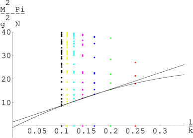
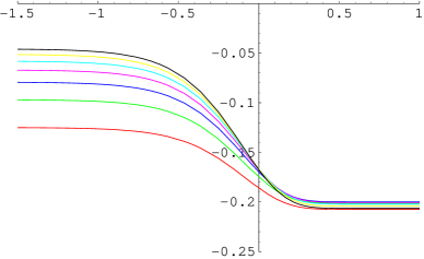
(a)	(b)

Figure 4: (a) The spectrum as a function of $1/k$ and (b) the Log-Log plot of the correlation function $\langle T^{++}(x)T^{++}(0)\rangle\left({x^{-}\over x^{+}}\right)^{2}{4\pi^{2}r^{4}\over N^{2}(2n_{b}+n_{f})}$ v.s. $r$ in the units where $g_{YM}^{2}N/\pi=1$ for $k=4\ldots 10$.

The spectrum of this theory at finite $k$, illustrated in figure 4.a, consists of $2k-2$ exactly massless states, accompanied by large numbers of massive states separated by a gap. The gap appears to be closing in the limit of large $k$ however. We have tried extrapolating the mass of the lightest massive state as a function of $1/k$ by performing a least square fit to a line and a parabola, giving the extrapolated value of $M^{2}\pi/g_{YM}^{2}N=1.7$ and $M^{2}\pi/g_{YM}^{2}N=-0.6$, suggesting indeed that at large $k$, the gap is closed. This is consistent with the expectation that the spectrum is that of a continuum starting at $M=0$ discussed earlier, although one must be careful when the order of large $N$ and large $k$ limits are exchanged. At finite $N$, we expect the degeneracy of $2k-2$ exactly massless states to be broken, giving rise to precisely a continuum of states starting at $M=0$ as expected.

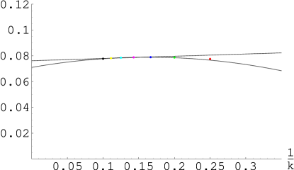
Figure 5: ${1\over k^{3}}\sum_{n}|{L\over\pi}\langle 0|T^{++}(k)|n\rangle|^{2}$ v.s. $k$ from states with $M|n\rangle=0$. This quantity determines the coefficient of the $1/r^{4}$ asymptotic tail of the correlation function in the large $r$ limit for the (1,1) model.

In the computation of the correlation function illustrated in figure 4.b, we find a curious feature that it asymptotes to the inverse power law $c/r^{4}$ for large $r$. This behavior comes about due to the coupling $\langle 0|T^{++}|n\rangle$ with exactly massless states $|n\rangle$. The contribution to (5.23) from strictly massless states are given by

$$\left(x^{-}\over x^{+}\right)^{2}F(x^{-},x^{+})=\left.\left|{L\over\pi}\langle 0|T^{++}(k)|n\rangle\right|^{2}{M_{n}^{4}\over 8\pi^{2}k^{3}}K_{4}(M_{n}r)\right|_{M_{n}=0}=$$ (5.31)

$$\left|{L\over\pi}\langle 0|T^{++}(k)|n\rangle\right|^{2}_{M_{n}=0}{6\over k^{3}\pi^{2}r^{4}}.$$

We have computed this quantity as a function of $1/k$ and extrapolated to $1/k\rightarrow 0$ by fitting a line and a parabola to the computed values for finite $1/k$. The result of this extrapolation is illustrated in figure 5. The data currently available suggests that the non-zero contribution from these massless states persists in the large $k$ limit.

Let us now turn to the model with (2,2) supersymmetry. The SDLCQ version of this model was solved in [11]. The result of this computation can be applied to (5.23). The result is summarized in figure 6. This model appears to exhibit the onset of a gapless continuum of states more rapidly than the (1,1) model as the harmonic resolution $k$ is increased. Just as we found in the (1,1) model, this theory contains exactly massless states in the spectrum. These massless states appear to couple to $T^{++}|0\rangle$ only for $k$ even, and the overlap appears to be decreasing as $k$ is increased. We believe that this model is likely to exhibit a power law behavior $c/r^{\gamma}$ for $\gamma>4$ for the $T^{++}$ correlator for $r\gg g_{YM}\sqrt{N}$ in the large $N$ limit. Unfortunately, the existing numerical data do not permit the reliable computation of the exponent $\gamma$.

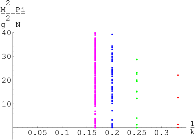
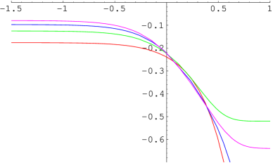
(a)	(b)

Figure 6: (a) The spectrum as a function of $1/k$ and (b) the Log-Log plot of the correlation function $\langle T^{++}(x)T^{++}(0)\rangle\left({x^{-}\over x^{+}}\right)^{2}{4\pi^{2}r^{4}\over N^{2}(2n_{b}+n_{f})}$ v.s. $r$ in the units where $g_{YM}^{2}N/\pi=1$ for $k=3\ldots 6$.

6 Bound States of Three Dimensional Supersymmetric Theory.

Recently, there has been considerable progress in understanding the properties of strongly coupled gauge theories with supersymmetry [75, 74]. In particular, there are a number of supersymmetric gauge theories that are believed to be inter-connected through a web of strong-weak coupling dualities. Although these dualities provide a deep insight into the dynamics of gauge theory at strong and weak couplings, they do not usually give much information about the spectrum of bound states at intermediate values of coupling constant $g$. The prominent exception is so called BPS states whose mass is protected by supersymmetry and thus stays the same for all values of $g$. An interesting new possibility for analytical treatment of bound state problem in SYM_D is based on the duality between SYM and supergravity proposed by Maldacena [61] as discussed in the previous section. This idea was also exploited in [28] to get the glueball spectrum of three dimensional theory and the results agree with lattice calculations.

However it would be interesting to solve the bound state problem for SYM theory directly, starting from the first principles of quantum field theory. As we have seen in the previous sections the solution can be found for the various two dimensional theories by means of applying discrete light cone quantization. Evidently, it would be desirable to extend these DLCQ/SDLCQ algorithms to solve higher dimensional theories. One important difference between two dimensional and higher dimensional theories is the phase diagram induced by variations in the gauge coupling. The spectrum of a $1+1$ dimensional gauge theory scales trivially with respect to the gauge coupling, while a theory in higher dimensions has the potential of exhibiting a complex phase structure, which may include a strong-weak coupling duality. It is therefore interesting to study the phase diagram of gauge theories in $D\geq 3$ dimensions.

Towards this end, we consider three dimensional SU($N$) ${\cal N}=1$ super-Yang-Mills compactified on the space-time ${\bf R}\times S^{1}\times S^{1}$. In particular, we compactify the light-cone coordinate $x^{-}$ on a light-like circle via DLCQ, and wrap the remaining transverse coordinate $x^{\perp}$ on a spatial circle. By retaining only the first few excited modes in the transverse direction, we are able to solve for bound state wave functions and masses numerically by diagonalizing the discretized light-cone supercharge. We show that the supersymmetric formulation of the DLCQ procedure – which was studied in the context of two dimensional theories extends naturally in $2+1$ dimensions, resulting in an exactly supersymmetric spectrum.

6.1 Light-Cone Quantization and SDLCQ

We wish to study the bound states of ${\cal N}=1$ super-Yang-Mills in $2+1$ dimensions. Any numerical approach necessarily involves introducing a momentum lattice – i.e. parton momenta can only take on discretized values. The usual space–time lattice explicitly breaks supersymmetry, so if we wish to discretize our theory and preserve supersymmetry, then a judicious choice of lattice is required.

In $1+1$ dimensions, it is well known that the light-cone momentum lattice induced by the DLCQ procedure preserves supersymmetry if the supercharge rather than the Hamiltonian is discretized [64, 7]. In $2+1$ dimensions, a supersymmetric prescription is also possible. We begin by introducing light-cone coordinates $x^{\pm}=(x^{0}\pm x^{1})/\sqrt{2}$, and compactifying the $x^{-}$ coordinate on a light-like circle. In this way, the conjugate light-cone momentum $k^{+}$ is discretized. To discretize the remaining (transverse) momentum $k^{\perp}=k^{2}$, we may compactify $x^{\perp}=x^{2}$ on a spatial circle. Of course, there is a significant difference between the discretized light-cone momenta $k^{+}$, and discretized transverse momenta $k_{\perp}$; namely, the light-cone momentum $k^{+}$ is always positive, while $k_{\perp}$ may take on positive or negative values. The positivity of $k^{+}$ is a key property that is exploited in DLCQ calculations; for any given light-cone compactification, there are only a finite number of choices for $k^{+}$ – the total number depending on how finely we discretize the momenta. In the context of two dimensional theories, this implies a finite number of Fock states [68].

In the case we are interested in – in which there is an additional transverse dimension – the number of Fock states is no longer finite, since there are an arbitrarily large number of transverse momentum modes defined on the transverse spatial circle. Thus, an additional truncation of the transverse momentum modes is required to render the total number of Fock states finite, and the problem numerically tractable. In this work, we choose the simplest truncation procedure beyond retaining the zero mode; namely, only partons with transverse momentum $k_{\perp}=0,\pm\frac{2\pi}{L}$ will be allowed, where $L$ is the size of the transverse circle.

Let us now apply these ideas in the context of a specific super-Yang-Mills theory. We start with $2+1$ dimensional ${\cal N}=1$ super-Yang-Mills theory defined on a space-time with one transverse dimension compactified on a circle:

$$S=\int d^{2}x\int_{0}^{L}dx_{\perp}\mbox{tr}(-\frac{1}{4}F^{\mu\nu}F_{\mu\nu}+{\rm i}{\bar{\Psi}}\gamma^{\mu}D_{\mu}\Psi).$$ (6.1)

After introducing the light–cone coordinates $x^{\pm}=\frac{1}{\sqrt{2}}(x^{0}\pm x^{1})$, decomposing the spinor $\Psi$ in terms of chiral projections –

$$\psi=\frac{1+\gamma^{5}}{2^{1/4}}\Psi,\qquad\chi=\frac{1-\gamma^{5}}{2^{1/4}}\Psi$$ (6.2)

and choosing the light–cone gauge $A^{+}=0$, the action becomes

$$S = \int dx^{+}dx^{-}\int_{0}^{L}dx_{\perp}\mbox{tr}\left[\frac{1}{2}(\partial_{-}A^{-})^{2}+D_{+}\phi\partial_{-}\phi+{\rm i}\psi D_{+}\psi+\right.$$ (6.3)

$$\left.\hskip 42.67912pt+{\rm i}\chi\partial_{-}\chi+\frac{{\rm i}}{\sqrt{2}}\psi D_{\perp}\phi+\frac{{\rm i}}{\sqrt{2}}\phi D_{\perp}\psi\right].$$

A simplification of the light–cone gauge is that the non-dynamical fields $A^{-}$ and $\chi$ may be explicitly solved from their Euler-Lagrange equations of motion:

$$A^{-} = \frac{g}{\partial_{-}^{2}}J=\frac{g}{\partial_{-}^{2}}\left(i[\phi,\partial_{-}\phi]+2\psi\psi\right),$$ (6.4)

$$\chi = -\frac{1}{\sqrt{2}\partial_{-}}D_{\perp}\psi.$$

These expressions may be used to express any operator in terms of the physical degrees of freedom only. In particular, the light-cone energy, $P^{-}$, and momentum operators, $P^{+}$,$P^{\perp}$, corresponding to translation invariance in each of the coordinates $x^{\pm}$ and $x_{\perp}$ may be calculated explicitly:

$$P^{+} = \int dx^{-}\int_{0}^{L}dx_{\perp}\mbox{tr}\left[(\partial_{-}\phi)^{2}+{\rm i}\psi\partial_{-}\psi\right],$$ (6.5)

$$P^{-} = \int dx^{-}\int_{0}^{L}dx_{\perp}\mbox{tr}\left[-\frac{g^{2}}{2}J\frac{1}{\partial_{-}^{2}}J-\frac{{\rm i}}{2}D_{\perp}\psi\frac{1}{\partial_{-}}D_{\perp}\psi\right],$$ (6.6)

$$P_{\perp} = \int dx^{-}\int_{0}^{L}dx_{\perp}\mbox{tr}\left[\partial_{-}\phi\partial_{\perp}\phi+{\rm i}\psi\partial_{\perp}\psi\right].$$ (6.7)

The light-cone supercharge in this theory is a two component Majorana spinor, and may be conveniently decomposed in terms of its chiral projections:

$$Q^{+} = 2^{1/4}\int dx^{-}\int_{0}^{L}dx_{\perp}\mbox{tr}\left[\phi\partial_{-}\psi-\psi\partial_{-}\phi\right],$$ (6.8)

$$Q^{-} = 2^{3/4}\int dx^{-}\int_{0}^{L}dx_{\perp}\mbox{tr}\left[2\partial_{\perp}\phi\psi+g\left({\rm i}[\phi,\partial_{-}\phi]+2\psi\psi\right)\frac{1}{\partial_{-}}\psi\right].$$ (6.9)

The action (6.3) gives the following canonical (anti)commutation relations for propagating fields at equal $x^{+}$:

$$\left[\phi_{ij}(x^{-},x_{\perp}),\partial_{-}\phi_{kl}(y^{-},y_{\perp})\right] = \frac{1}{2}{\rm i}\delta(x^{-}-y^{-})\delta(x_{\perp}-y_{\perp})\left(\delta_{il}\delta_{jk}-\frac{1}{N}\delta_{ij}\delta_{kl}\right),$$ (6.10)

$$\left\{\psi_{ij}(x^{-},x_{\perp}),\psi_{kl}(y^{-},y_{\perp})\right\} = \frac{1}{2}\delta(x^{-}-y^{-})\delta(x_{\perp}-y_{\perp})\left(\delta_{il}\delta_{jk}-\frac{1}{N}\delta_{ij}\delta_{kl}\right).$$ (6.11)

Using these relations one can check the supersymmetry algebra:

$$\{Q^{+},Q^{+}\}=2\sqrt{2}P^{+},\qquad\{Q^{-},Q^{-}\}=2\sqrt{2}P^{-},\qquad\{Q^{+},Q^{-}\}=-4P_{\perp}.$$ (6.12)

We will consider only states which have vanishing transverse momentum, which is possible since the total transverse momentum operator is kinematical. On such states, the light-cone supercharges $Q^{+}$ and $Q^{-}$ anti-commute with each other, and the supersymmetry algebra is equivalent to the ${\cal N}=(1,1)$ supersymmetry of the dimensionally reduced (i.e. two dimensional) theory [64]. Moreover, in the $P_{\perp}=0$ sector, the mass squared operator $M^{2}$ is given by $M^{2}=2P^{+}P^{-}$.

As we mentioned earlier, in order to render the bound state equations numerically tractable, the transverse momentum of partons must be truncated. First, we introduce the Fourier expansion for the fields $\phi$ and $\psi$, where the transverse space-time coordinate $x^{\perp}$ is periodically identified:

$$\phi_{ij}(0,x^{-},x_{\perp})=$$

$$\frac{1}{\sqrt{2\pi L}}\sum_{n^{\perp}=-\infty}^{\infty}\int_{0}^{\infty}\frac{dk^{+}}{\sqrt{2k^{+}}}\left[a_{ij}(k^{+},n^{\perp})e^{-{\rm i}k^{+}x^{-}-{\rm i}\frac{2\pi n^{\perp}}{L}x_{\perp}}+a^{\dagger}_{ji}(k^{+},n^{\perp})e^{{\rm i}k^{+}x^{-}+{\rm i}\frac{2\pi n^{\perp}}{L}x_{\perp}}\right]$$

$$\psi_{ij}(0,x^{-},x_{\perp})=$$

$$\frac{1}{2\sqrt{\pi L}}\sum_{n^{\perp}=-\infty}^{\infty}\int_{0}^{\infty}dk^{+}\left[b_{ij}(k^{+},n^{\perp})e^{-{\rm i}k^{+}x^{-}-{\rm i}\frac{2\pi n^{\perp}}{L}x_{\perp}}+b^{\dagger}_{ji}(k^{+},n^{\perp})e^{{\rm i}k^{+}x^{-}+{\rm i}\frac{2\pi n^{\perp}}{L}x_{\perp}}\right]$$

Substituting these into the (anti)commutators (6.11), one finds:

$$\left[a_{ij}(p^{+},n_{\perp}),a^{\dagger}_{lk}(q^{+},m_{\perp})\right] = \delta(p^{+}-q^{+})\delta_{n_{\perp},m_{\perp}}\left(\delta_{il}\delta_{jk}-\frac{1}{N}\delta_{ij}\delta_{lk}\right)$$ (6.13)

$$\left\{b_{ij}(p^{+},n_{\perp}),b^{\dagger}_{lk}(q^{+},m_{\perp})\right\} = \delta(p^{+}-q^{+})\delta_{n_{\perp},m_{\perp}}\left(\delta_{il}\delta_{jk}-\frac{1}{N}\delta_{ij}\delta_{lk}\right).$$ (6.14)

The supercharges now take the following form:

$$Q^{+}={\rm i}2^{1/4}\sum_{n^{\perp}\in{\bf Z}}\int_{0}^{\infty}dk\sqrt{k}\left[b_{ij}^{\dagger}(k,n^{\perp})a_{ij}(k,n^{\perp})-a_{ij}^{\dagger}(k,n^{\perp})b_{ij}(k,n^{\perp})\right],$$ (6.15)

$$Q^{-}=\frac{2^{7/4}\pi{\rm i}}{L}\sum_{n^{\perp}\in{\bf Z}}\int_{0}^{\infty}dk\frac{n^{\perp}}{\sqrt{k}}\left[a_{ij}^{\dagger}(k,n^{\perp})b_{ij}(k,n^{\perp})-b_{ij}^{\dagger}(k,n^{\perp})a_{ij}(k,n^{\perp})\right]+$$

$$+{{\rm i}2^{-1/4}{g}\over\sqrt{L\pi}}\sum_{n^{\perp}_{i}\in{\bf Z}}\int_{0}^{\infty}dk_{1}dk_{2}dk_{3}\delta(k_{1}+k_{2}-k_{3})\delta_{n^{\perp}_{1}+n^{\perp}_{2},n^{\perp}_{3}}\left\{\frac{}{}\right.$$

$${1\over 2\sqrt{k_{1}k_{2}}}{k_{2}-k_{1}\over k_{3}}[a_{ik}^{\dagger}(k_{1},n^{\perp}_{1})a_{kj}^{\dagger}(k_{2},n^{\perp}_{2})b_{ij}(k_{3},n^{\perp}_{3})-b_{ij}^{\dagger}(k_{3},n^{\perp}_{3})a_{ik}(k_{1},n^{\perp}_{1})a_{kj}(k_{2},n^{\perp}_{2})]$$

$${1\over 2\sqrt{k_{1}k_{3}}}{k_{1}+k_{3}\over k_{2}}[a_{ik}^{\dagger}(k_{3},n^{\perp}_{3})a_{kj}(k_{1},n^{\perp}_{1})b_{ij}(k_{2},n^{\perp}_{2})-a_{ik}^{\dagger}(k_{1},n^{\perp}_{1})b_{kj}^{\dagger}(k_{2},n^{\perp}_{2})a_{ij}(k_{3},n^{\perp}_{3})]$$

$${1\over 2\sqrt{k_{2}k_{3}}}{k_{2}+k_{3}\over k_{1}}[b_{ik}^{\dagger}(k_{1},n^{\perp}_{1})a_{kj}^{\dagger}(k_{2},n^{\perp}_{2})a_{ij}(k_{3},n^{\perp}_{3})-a_{ij}^{\dagger}(k_{3},n^{\perp}_{3})b_{ik}(k_{1})a_{kj}(k_{2},n^{\perp}_{2})]$$

$$({1\over k_{1}}+{1\over k_{2}}-{1\over k_{3}})[b_{ik}^{\dagger}(k_{1},n^{\perp}_{1})b_{kj}^{\dagger}(k_{2},n^{\perp}_{2})b_{ij}(k_{3},n^{\perp}_{3})+b_{ij}^{\dagger}(k_{3},n^{\perp}_{3})b_{ik}(k_{1},n^{\perp}_{1})b_{kj}(k_{2},n^{\perp}_{2})]\left.\frac{}{}\right\}.$$

We now perform the truncation procedure; namely, in all sums over the transverse momenta $n^{\perp}_{i}$ appearing in the above expressions for the supercharges, we restrict summation to the following allowed momentum modes: $n^{\perp}_{i}=0,\pm 1$. More generally, the truncation procedure may be defined by $|n^{\perp}_{i}|\leq N_{max}$, where $N_{max}$ is some positive integer. In this work, we consider the simple case $N_{max}=1$. Note that this prescription is symmetric, in the sense that there are as many positive modes as there are negative ones. In this way we retain parity symmetry in the transverse direction.

How does such a truncation affect the supersymmetry properties of the theory? Note first that an operator relation $[A,B]=C$ in the full theory is not expected to hold in the truncated formulation. However, if A is quadratic in terms of fields (or in terms of creation and annihilation operators), one can show that the relation $[A,B]=C$ implies

$$[A_{tr},B_{tr}]=C_{tr}$$

for the truncated operators $A_{tr}$,$B_{tr}$, and $C_{tr}$. In our case, $Q^{+}$ is quadratic, and so the relations $\{Q_{tr}^{+},Q_{tr}^{+}\}=2\sqrt{2}P_{tr}^{+}$ and $\{Q_{tr}^{+},Q_{tr}^{-}\}=0$ are true in the $P_{\perp}=0$ sector of the truncated theory. The $\{Q_{tr}^{-},Q_{tr}^{-}\}$ however is not equal to $2\sqrt{2}P_{tr}^{-}$. So the diagonalization of $\{Q_{tr}^{-},Q_{tr}^{-}\}$ will yield a different bound state spectrum than the one obtained after diagonalizing $2\sqrt{2}P_{tr}^{-}$. Of course the two spectra should agree in the limit $N_{max}\rightarrow\infty$. At any finite truncation, however, we have the liberty to diagonalize any one of these operators. This choice specifies our regularization scheme.

Choosing to diagonalize the light-cone supercharge, however, has an important advantage: the spectrum is exactly supersymmetric for any truncation. In contrast, the spectrum of the Hamiltonian becomes supersymmetric only in the $N_{max}\rightarrow\infty$ limit.

To summarize, we have introduced a truncation procedure that facilitates a numerical study of the bound state problem, and preserves supersymmetry. The interesting property of the light-cone supercharge $Q^{-}$ [Eqn(6.1)] is the presence of a gauge coupling constant as an independent variable, which does not appear in the study of two dimensional theories. In the next subsection, we will study how variations in this coupling affects the bound states in the theory.

6.2 Numerical Results: Bound State Solutions

In order to implement the DLCQ formulation of the bound state problem – which is tantamount to imposing periodic boundary conditions $x^{-}=x^{-}+2\pi R$ [63] – we simply restrict the light-cone momentum variables $k_{i}$ appearing in the expressions for $Q^{+}$ and $Q^{-}$ to the following discretized set of momenta: $\left\{\frac{1}{K}P^{+},\frac{2}{K}P^{+},\frac{3}{K}P^{+},\dots,\right\}$. Here, $P^{+}$ denotes the total light-cone momentum of a state, and may be thought of as a fixed constant, since it is easy to form a Fock basis that is already diagonal with respect to the operator $P^{+}$ [68]. The integer $K$ is called the ‘harmonic resolution’, and $1/K$ measures the coarseness of our discretization. The continuum limit is then recovered by taking the limit $K\rightarrow\infty$. Physically, $1/K$ represents the smallest positive unit of longitudinal momentum-fraction allowed for each parton in a Fock state.

Figure 7: Plot of bound state mass squared $M^{2}$ in units $16\pi^{2}N/L^{2}$ as a function of the dimensionless coupling $0\leq g^{\prime}\leq 2$, defined by $(g^{\prime})^{2}=g^{2}NL/16\pi^{3}$, at $N=1000$ and $K=5$. Boson and fermion masses are identical.

Of course, as soon as we implement the DLCQ procedure, which is specified unambiguously by the harmonic resolution $K$, and cut-off transverse momentum modes via the constraint $|n_{i}^{\perp}|\leq N_{max}$, the integrals appearing in the definitions for $Q^{+}$ and $Q^{-}$ are replaced by finite sums, and so the eigen-equation $2P^{+}P^{-}|\Psi\rangle=M^{2}|\Psi\rangle$ is reduced to a finite matrix diagonalization problem. In this last step we use the fact that $P^{-}$ is proportional to the square of the light-cone supercharge $Q^{-}$. In the present work, we are able to perform numerical diagonalizations for $K=2,3,4$ and $5$ with the help of Mathematica and a desktop PC.

Figure 8: Plot of bound state mass squared $M^{2}$ in units $16\pi^{2}N/L^{2}$ as a function of the dimensionless coupling $0\leq g^{\prime}\leq 10$, defined by $(g^{\prime})^{2}=g^{2}NL/16\pi^{3}$, at $N=1000$ and $K=5$. Note the appearance of a new massless state at strong coupling.

In Figure 7, we plot the bound state mass squared $M^{2}$, in units $16\pi^{2}N/L^{2}$, as a function of the dimensionless coupling $g^{\prime}=g\sqrt{NL}/4\pi^{3/2}$, in the range $0\leq g^{\prime}\leq 2$. We consider the specific case $N=1000$, although our algorithm can calculate masses for any choice of $N$, since it enters our calculations as an algebraic variable. Since there is an exact boson-fermion mass degeneracy, one needs only diagonalize the mass matrix $M^{2}$ corresponding to the bosons. For $K=5$, there are precisely 600 bosons and 600 fermions in the truncated light-cone Fock space, so the mass matrix that needs to be diagonalized has dimensions $600\times 600$. At $K=4$, there are $92$ bosons and $92$ fermions, while at $K=3$, one finds $16$ bosons and $16$ fermions.

In Figure 8, we plot the bound state spectrum in the range $0\leq g^{\prime}\leq 10$. It is apparent now that new massless states appear in the strong coupling limit $g^{\prime}\rightarrow\infty$.

Figure 9: Plot of average length for the eight massless bosonic states as a function of the dimensionless coupling $g^{\prime}$, defined by $(g^{\prime})^{2}=g^{2}NL/16\pi^{3}$, at $N=1000$ and $K=5$. Note that the states attain the maximum possible length allowed by the resolution $K=5$ in the limit of strong coupling.

An interesting property of the spectrum is the presence of exactly massless states that persist for all values of the coupling $g^{\prime}$. For $K=5$, there are 16 such states (8 bosons and 8 fermions). At $K=4$, one finds 8 states (4 bosons and 4 fermions) that are exactly massless for any coupling, while for $K=3$, there are 4 states (two bosons and two fermions) with this property. We will have more to say regarding these states in the next subsection, but here we note that the structure of these states become ‘string-like’ in the strong coupling limit. This is illustrated in Figure 9, where we plot the ‘average length’ (or average number of partons) of each of these massless states. This quantity is obtained by counting the number of partons in each Fock state that comprises a massless bound state, appropriately weighted by the modulus of the wave function squared. Clearly, at strong coupling, the average number of partons saturates the maximum possible value allowed by the resolution – in this case 5 partons. The same behavior is observed at lower resolutions. Thus, in the continuum limit $K\rightarrow\infty$, we expect the massless states in this theory to become string-like at strong coupling.

Comparison Between $1+1$ and $2+1$ Spectra
-	$1+1$ Model	Rescaled $2+1$ Model
$K$	-	$g^{\prime}=.01$	$g^{\prime}=.1$	$g^{\prime}=1.0$
$K=5$	15.63	15.5	15.17	3.7
	18.23	17.6	17.9	3.5
	21.8	21.3	21.7	3.2
$K=4$	-	-	-	-
	18.0	17.99	17.6	3.56
	21.3	21.3	21.0	3.1
$K=3$	-	-	-	-
	-	-	-	-
	20.2	20.2	19.8	3.1

Table 2: Values for the mass squared $M^{2}$, in units ${\tilde{g}}^{2}N/\pi$, with ${\tilde{g}}^{2}=g^{2}/L$, for bound states in the dimensionally reduced ${\cal N}=(1,1)$ model, and the $2+1$ model studied here. The quantity ${\tilde{g}}$ is identified as the gauge coupling in the $1+1$ model. We set $K=3,4$ and $5$, and $N=1000$. Note that the comparison of masses between the $1+1$ model, and the (re-scaled) $2+1$ model is good only at weak coupling $g^{\prime}$.

One interesting property of the model studied here is the manifest ${\cal N}=(1,1)$ supersymmetry in the $P^{\perp}=0$ momentum sector, by virtue of the supersymmetry relations (6.12). Moreover, if we consider retaining only the zero mode $n_{i}^{\perp}=0$, then the light-cone supercharge $Q^{-}$ for the $2+1$ model is identical to the $1+1$ dimensional ${\cal N}=(1,1)$ supersymmetric Yang-Mills theory studied in [64, 5, 6], after a rescaling by the factor $1/g^{\prime}$. (This is equivalent to expressing the mass squared $M^{2}$ in units ${\tilde{g}}^{2}N/\pi$, where ${\tilde{g}}=g/\sqrt{L}$. The quantity ${\tilde{g}}$ is then identified as the gauge coupling in the $1+1$ theory.) We may therefore think of the additional transverse degrees of freedom in the $2+1$ model, represented by the modes $n^{\perp}=\pm 1$, as a modification of the $1+1$ model. A natural question that follows from this viewpoint is: How well does the $1+1$ spectrum approximate the $2+1$ spectrum after performing this rescaling? Before discussing the numerical results summarized in Table 2, let us first attempt to predict what will happen at small coupling $g^{\prime}$. In this case, the coefficients of terms in the rescaled Hamiltonian $P^{-}$ that correspond to summing the transverse momentum squared $|k^{\perp}|^{2}$ of partons in a state will be large. So the low energy sector will be dominated by states with $n^{\perp}=0$. i.e. those states that appear in the Fock space of the ${\cal N}=(1,1)$ model in $1+1$ dimensions. This is indeed supported by the results in Table 2.

For large coupling $g^{\prime}$, however, it is clear that the approximation breaks down. In fact, one can show that the tabulated masses in the rescaled $2+1$ model tend to zero in the strong coupling limit, which eliminates any scope for making comparisons between the two and three dimensional models.

Thus, the non-perturbative problem of solving dimensionally reduced models in $1+1$ dimensions can only provide information about bound state masses in the corresponding weakly coupled higher dimensional theory.

6.3 Analytical Results: The Massless Sector

In the previous subsection we presented the results of studying the bound state problem using numerical methods. In performing such a study we conveniently chose the simplest nontrivial truncation of the transverse momentum modes; namely, $n_{\perp}=0,\pm 1$. Surprisingly, such a simple scheme provided many interesting insights concerning the massless and massive sector. In particular we see that there are three types of massless states; those that are massless only at $g=0$ or $g=\infty$ (but not both), and those that are massless for any value of the coupling. In this subsection, we will analyze only the massless sector of the theory, and show that the observed properties of the spectrum with the truncation $n^{\perp}=0,\pm 1$ also persists if we include higher modes: $n^{\perp}=0,\pm 1,\pm 2,\dots,\pm N_{max}$. We therefore consider the model with supercharges given by (6.15) and (6.1), and restrict summation of transverse momentum modes via the constraint $|n^{\perp}|\leq N_{max}$.

For states carrying positive light-cone momentum, $P^{+}$ is never zero, and so massless states must satisfy the equation $P^{-}|\Psi\rangle=0$, which, using the relation $P^{-}=\frac{1}{\sqrt{2}}(Q^{-})^{2}$, and hermiticity of $Q^{-}$, reduces to

$$Q^{-}|\Psi\rangle=0.$$ (6.17)

This is the equation we wish to study in detail.

We begin with an analysis of the weak coupling limit of the theory. This limit means that the dimensionless coupling constant is small: i.e. $g\sqrt{L}\ll 1$. We will consider the strong–weak coupling behavior of the theory on a cylinder with fixed circumference $L$ so it is convenient to choose the units in which $L=1$ for this discussion. The supercharge (6.1) consists of two parts: one is proportional to the coupling and the other is coupling–independent:

$$Q^{-}=Q_{\perp}+g{\tilde{Q}}.$$ (6.18)

So at $g=0$, the equation (6.17) reduces to $Q_{\perp}|\Psi\rangle=0$, which means that $|\Psi\rangle$ may be viewed as a state in the Fock space of the two dimensional ${\cal N}=(1,1)$ super Yang-Mills theory, which may be obtained by dimensional reduction of the $2+1$ theory. Thus the massless states at $g=0$ are states with any combination of $a^{\dagger}(k,0)$ and $b^{\dagger}(k,0)$ modes, and no partons with nonzero transverse momentum.

What happens with these massless states when one switches on the coupling? To answer this question, we need some information about the behavior of states as functions of the coupling. We assume that wave functions are analytic in terms of $g$ at least in the vicinity of $g=0$. This means that in this region any massless state $|\Psi\rangle$ may be written in the form:

$$|\Psi\rangle=\sum_{n=0}^{\infty}g^{n}|n\rangle,$$ (6.19)

where states $|n\rangle$ are coupling independent. Then using relation (6.18), the $g$–dependent equation (6.17) may be written as an infinite system of relations between different $|n\rangle$:

$$Q_{\perp}|0\rangle=0,$$ (6.20)

$$Q_{\perp}|n\rangle+{\tilde{Q}}|n-1\rangle=0,\qquad n>0.$$ (6.21)

The first of these equations was already used to exclude partons carrying non-zero transverse momentum, which is a property of the massless bound states at zero coupling. The second equation is non-trivial. Let us consider two different subspaces in the theory. The first of these subspaces consists of states with no creation operators for transverse modes which we will label $1$. The other is the complement of this space in which the operator $Q_{\perp}$ is invertible and we label this space 2. Equation (6.21) defines the recurrence relation when ${\tilde{Q}}|n-1\rangle$ is in subspace $2$:

$$|n\rangle=-Q_{\perp}^{-1}\left(\left.{\tilde{Q}}|n-1\rangle\right|_{2}\right),$$ (6.22)

The consistency condition is that projection of ${\tilde{Q}}|n-1\rangle$ in subspace $1$ is zero,

$$\left.{\tilde{Q}}|n-1\rangle\right|_{1}=0.$$ (6.23)

This condition implies that not all states of the two dimension theory, $g=0$ , may be extended to such states at arbitrary $g$ using (6.22). Taking $n=1$, (6.23) implies that $|0\rangle$ is a massless state of the dimensionally reduced theory. The numerical solutions, of course, show this correspondence between the $2+1$ and $1+1$[64, 5, 6] massless bound states. Starting from a massless state of the two dimensional theory, and we construct states $|n\rangle$ using (6.22), and for which (6.23) is always satisfied. Then $|\Psi\rangle$ may be found from summing a geometric series:

$$|\Psi\rangle=\sum_{n=0}^{\infty}(-gQ_{\perp}^{-1}{\tilde{Q}})^{n}|0\rangle=\frac{1}{1+gQ_{\perp}^{-1}{\tilde{Q}}}|0\rangle.$$ (6.24)

So, starting from the massless state of the two dimensional ${\cal N}=(1,1)$ model, one can always construct unique massless states in the three dimensional theory at least in the vicinity of $g=0$.

The state (6.24) turns out to be massless for any value of the coupling:

$$Q^{-}|\Psi\rangle=Q_{\perp}(1+gQ_{\perp}^{-1}{\tilde{Q}})\frac{1}{1+gQ_{\perp}^{-1}{\tilde{Q}}}|0\rangle=Q_{\perp}|0\rangle=0,$$ (6.25)

though the state itself is dependent on g. Thus, we have shown that massless states of the three dimensional theory, at nonzero coupling, can be constructed from massless states of the corresponding model in two dimensions. All other states containing only two dimensional modes can also be extended to the eigenstates of the full theory. But such eigenstates are massless only at zero coupling. Assuming analyticity, one can then show that their masses grow linearly at $g$ in the vicinity of zero. Such behavior also agrees with our numerical results.

To illustrate the general construction explained above we consider one simple example. Working in DLCQ at resolution $K=3$ we choose a special two dimensional massless state [64, 5, 6]:

$$|0\rangle=\mbox{tr}(a^{\dagger}(1,0)a^{\dagger}(2,0))|vac\rangle.$$ (6.26)

Then in the SU($N$) theory we find:

$${\tilde{Q}}|0\rangle = \frac{3}{2\sqrt{2}}\left[\mbox{tr}\left(a^{\dagger}(1,0)(b^{\dagger}(1,-1)a^{\dagger}(1,1)-a^{\dagger}(1,1)b^{\dagger}(1,-1)+\right.\right.$$ (6.27)

$$+ \left.\left.b^{\dagger}(1,1)a^{\dagger}(1,-1)-a^{\dagger}(1,-1)b^{\dagger}(1,1))\right)\right]|vac\rangle,$$

$$|1\rangle = -Q_{\perp}^{-1}{\tilde{Q}}|0>=-\frac{\sqrt{L}}{4\pi^{3/2}}\frac{3}{2\sqrt{2}}\left(a^{\dagger}(1,0)a^{\dagger}(1,-1)a^{\dagger}(1,1)-\right.$$ (6.28)

$$- \left.a^{\dagger}(1,0)a^{\dagger}(1,1)a^{\dagger}(1,-1)\right)|vac\rangle$$

$${\tilde{Q}}|1\rangle = 0.$$ (6.29)

The last equation provides the consistency condition (6.23) for $n=2$, and it also shows that for this special example we have only two states $|0\rangle$ and $|1\rangle$, instead of a general infinite set. The matrix form of the operator $1+gQ_{\perp}^{-1}{\tilde{Q}}$ in the $|0\rangle,|1\rangle$ basis is

$$1+gQ_{\perp}^{-1}{\tilde{Q}}=\left(\begin{array}[]{cc}1&-g\\ 0&1\end{array}\right)=\left(\begin{array}[]{cc}1&g\\ 0&1\end{array}\right)^{-1}.$$ (6.30)

Then the solution of (6.24) is

$$|\Psi\rangle=|0\rangle+g|1\rangle=\mbox{tr}(a^{\dagger}(1,0)a^{\dagger}(2,0))|vac\rangle+$$ (6.31)

$$+\frac{g\sqrt{L}}{4\pi^{3/2}}\frac{3}{2\sqrt{2}}\left(a^{\dagger}(1,0)a^{\dagger}(1,1)a^{\dagger}(1,-1)-a^{\dagger}(1,0)a^{\dagger}(1,-1)a^{\dagger}(1,1)\right)|vac\rangle.$$

This state was observed numerically, and the dependence of the wave function on the coupling constant is precisely the one given by the last formula.

In principle, we can determine the wave functions of all massless states using this formalism. Our procedure has an important advantage over a direct diagonalization of the three dimensional supercharge. Firstly, in order to find two dimensional massless states, one needs to diagonalize the corresponding supercharge [64]. However, the dimension of the relevant Fock space is much less than the three dimensional theory (at large resolution $K$, the ratio of these dimensions is of order $(N_{max}+1)^{\alpha K}$, $\alpha\sim 1/4$). The extension of the two dimensional massless solution into a massless solution of the three dimensional theory requires diagonalizing a matrix which has a smaller dimension than the original problem in three dimensions. Thus, if one is only interested in the massless sector of the three dimensional theory, the most efficient way to proceed in DLCQ calculations is to solve the two dimensional theory, and then to upgrade the massless states to massless solutions in three dimensions.

Finally, we will make some comments on bound states at very strong coupling. Of course, we have states (6.24) which are massless at any coupling, but our numerical calculation show there are additional states which become massless at $g=\infty$ (see Figure 8). To discuss these state it is convenient to consider

$${\bar{Q}}^{-}=\frac{1}{g}Q_{\perp}+{\tilde{Q}}$$ (6.32)

instead of $Q^{-}$, and perform the strong coupling expansion. Since we are interested only in massless states, the absolute normalization doesn’t matter. We repeat all the arguments used in the weak coupling case: first, we introduce the space $1^{*}$ where ${\tilde{Q}}$ can not be inverted, and its orthogonal complement $2^{*}$. Then any state from $1^{*}$ is massless at $g=\infty$, but assuming the expansion

$$|\Psi\rangle=\sum_{n=0}^{\infty}\frac{1}{g^{n}}|n\rangle^{*}$$ (6.33)

at large enough $g$, one finds the analogs of (6.22) and (6.23):

$$|n\rangle^{*}=-{\tilde{Q}}^{-1}\left(\left.Q_{\perp}|n-1\rangle^{*}\right|_{2^{*}}\right),$$ (6.34)

$$\left.Q_{\perp}|n-1\rangle^{*}\right|_{1^{*}}=0.$$ (6.35)

As in the small coupling case, there are two possibilities: either one can construct all states $|n\rangle^{*}$ satisfying the consistency conditions, or at least one of these conditions fails. The former case corresponds to the massless state in the vicinity of $g=\infty$, which can be extended to the massless states at all couplings. The states constructed in this way – and ones given by (6.24) – define the same subspace. In the latter case, the state is massless at $g=\infty$, but it acquires a mass at finite coupling. There is a big difference, however, between the weak and strong coupling cases. While the kernel of $Q_{\perp}$ consists of ”two dimensional” states, the description of the states annihilated by ${\tilde{Q}}$ is a nontrivial dynamical problem. Since the massless states can be constructed starting from either $g=0$ or $g=\infty$, we don’t have to solve this problem to build them. If, however, one wishes to show that massless states become long in the strong coupling limit (there is numerical evidence for such behavior – see Figure 9), the structure of $1^{*}$ space becomes important, and we leave this question for future investigation.

Conclusion.

In these lectures we have reviewed some of the progress in the application of discrete light cone quantization to supersymmetric systems. Studying such systems is especially interesting because the cancellation between bosonic and fermionic loops make these theories much easier to renormalize than the models without supersymmetry. Although we didn’t need this advantage when considering two dimensional systems, it becomes crucial in higher dimensions. From this point of view it is desirable to have exact SUSY in discretized theories to simplify the renormalization in DLCQ.

while we are still far from the point of solving the bound state problem in three and four dimensional theories, we can already make some statements about these theories. For example in section 2 we described the vacuum structure of $SYM_{2+1}$ on a cylinder. The reason for this is that only zero modes contribute to such structure, thus studying the theory dimensionally reduced to $1+1$ provide all the necessary information. As we saw in section 6, two dimensional models can also be used to determine the behavior of bound states at weak coupling in three dimensions and to count the exact massless states. We performed such counting only for (1,1) theory, the case of (2,2) supersymmetry [11] and the even more interesting case of the (8,8) theory [9] which is known to have a mass gap have not been addressed.

Let us now mention a few of the immediate challenges for SDLCQ. First of all is the extention of the numerical results of section 5 to higher resolution and thus to test the Maldacena’s conjecture. The only problem here is the limits in one’s computing resources and the the speed of the algorithems one uses. Impovements here will also help use to extend our analysis of higher dimensional system and to larger values of transverse truncation. Unfortunately the transverse truncation that we have achieved so far does not provide much information about behavior of the spectrum as a function of transverse resolution and was used mainly for illustration of the general concepts. Another consideration is that our approach studies theories on a light like cylinder and thus our theories may have as aspects in which they are different than theories in infinite spacetime or on a space like cylinder.

7 Acknowledgments

This work was supported in part by the US Department of Energy. All of the work reported in these lectures was done in collaboration with Francesco Antonuccio. We would like to acknowledge the other members of the SDLCQ project, S. Tsujimaru, C. Pauli, J. Hiller, Uwe Trittmann, and Igor Filippos.

References

- [1] S. Adler, “Axial vector vertex in spinor electrodynamics,” Phys. Rev. 177 (1969) 2426.
- [2] O. Aharony, S. S. Gubser, J. Maldacena, H. Ooguri, and Y. Oz, “Large N field theories, string theory and gravity,” hep-th/9905111.
- [3] F. Antonuccio, S.J. Brodsky, S. Dalley, ”Light-Cone Wavefunctions at Small ,” Phys.Lett. B412 (1997) 104.
- [4] F. Antonuccio, A. Hashimoto, O. Lunin, S. Pinsky, “Can DLCQ test the Maldacena Conjecture?”, JHEP 9907 (1999) 029, hep-th/9906087.
- [5] F. Antonuccio, O. Lunin, S. Pinsky, “Bound States of Dimensionally Reduced at Finite ”, Phys.Lett. B429 (1998) 327-335, hep-th/9803027.
- [6] F. Antonuccio, O. Lunin, and S. Pinsky, “Nonperturbative spectrum of two-dimensional (1,1) superYang-Mills at finite and large N,” Phys. Rev. D58 (1998) 085009, hep-th/9803170.
- [7] F. Antonuccio, O. Lunin, and S. Pinsky, “On Exact Supersymmetry in DLCQ,” Phys.Lett. B442 (1998) 173, hep-th/9809165.
- [8] F. Antonuccio, O. Lunin, and S. Pinsky, “Super Yang-Mills at Weak, Intermediate and Strong Coupling”, Phys.Rev. D D59 (1999) 085001, hep-th/9811083.
- [9] F. Antonuccio, O. Lunin, S. Pinsky, H. C. Pauli, and S. Tsujimaru, “The DLCQ spectrum of N=(8,8) superYang-Mills,” Phys. Rev. D58 (1998) 105024, hep-th/9806133.
- [10] F. Antonuccio, O. Lunin, S. Pinsky, and S. Tsujimaru, “The Light cone vacuum in (1+1)-dimensional superYang-Mills theory,” hep-th/9811254.
- [11] F. Antonuccio, H. C. Pauli, S. Pinsky, and S. Tsujimaru, “DLCQ bound states of N=(2,2) super Yang-Mills at finite and large N,” Phys. Rev. D58 (1998) 125006, hep-th/9808120.
- [12] F. Antonuccio, S.S. Pinsky, ”Matrix theories from reduced Yang–Mills with adjoint fermions,” Phys.Lett B397 (1997) 42, hep-th/9612021.
- [13] F. Antonuccio, S. Pinsky, ”On the transition from confinement to screening in QCD1+1 coupled to adjoint fermions at finite N, ” Phys.Lett. B439 (1998) 142, hep-th/9805188.
- [14] F. Antonuccio, S. Pinsky, and S. Tsujimaru, “A Comment on the light cone vacuum in (1+1)-dimensional superYang-Mills theory,” hep-th/9810158.
- [15] A. Armoni, Y. Frishman, and J. Sonnenschein, “Screening in supersymmetric gauge theories in two- dimensions,” Phys. Lett. B449 (1999) 76, hep-th/9807022.
- [16] A. Armoni, Y. Frishman, and J. Sonnenschein, “The String tension in two-dimensional gauge theories,” hep-th/9903153.
- [17] A. Armoni, J. Sonnenschein, “Screening and Confinement in Large and in ,” hep-th/9703114.
- [18] T. Banks, W. Fischler, S. Shenker, L. Susskind, ”M theory as a matrix model: a conjecture,” Phys. Rev. D55 (1997) 5112,hep--th/9610043.
- [19] C. Bender, S. Pinsky, B. van de Sande, “Spontaneous symmetry breaking of in light front field theory,” Phys. Rev. D48 (1993) 816.
- [20] G. Bhanot, K. Demeterfi, I.R. Klebanov, ”–Dimensional Large N QCD Coupled to Adjoint fermions,” Phys. Rev. D48 (1993) 4980, hep--th/9307111.
- [21] D. Bigatti, L. Susskind, ”Review of Matrix Theory,” hep-th/9712072.
- [22] D. Birmingham, M. Blau, M. Rakowski, and G. Thompson, “Topological field theory,” Phys. Rept. 209 (1991) 129–340.
- [23] J. Boorstein, D. Kutasov, ”Symmetries and mass splittings in QCD2 coupled to adjoint fermions,” Nucl.Phys. B421 (1994) 263, hep-th/9401044.
- [24] A. Brandhuber, N. Itzhaki, J. Sonnenschein, and S. Yankielowicz, “Wilson loops, confinement, and phase transitions in large N gauge theories from supergravity,” JHEP 06 (1998) 001, hep-th/9803263.
- [25] S. J. Brodsky, H.-C. Pauli, and S. S. Pinsky, “Quantum chromodynamics and other field theories on the light cone,” Phys. Rept. 301 (1998) 299, hep-ph/9705477.
- [26] M. Burkardt, F. Antonuccio, and S. Tsujimaru, “Decoupling of zero modes and covariance in the light front formulation of supersymmetric theories,” Phys. Rev. D58 (1998) 125005, hep-th/9807035.
- [27] C. G. Callan, N. Coote, and D. J. Gross, “Two-Dimensional Yang-Mills Theory: A Model of Quark Confinement,” Phys. Rev. D13 (1976) 1649.
- [28] C. Csaki, H. Ooguri, Y. Oz, J.Terning, “Glueball mass spectrum from supergravity,” JHEP 9901 (1999) 017, hep-th/9806021.
- [29] S. Dalley and I.R. Klebanov, ”String Spectrum of 1+1-Dimensional Large QCD with Adjoint Matter”, Phys. Rev. D47 (1993) 2517, hep-th/9209049.
- [30] K. Demeterfi and I. R. Klebanov, “Matrix models and string theory,”. Lectures given at Spring School on String Theory, Gauge Theory and Quantum Gravity, Trieste, Italy, 19-27 Apr 1993.
- [31] R. Dijkgraaf, E. Verlinde, and H. Verlinde, “Matrix string theory,” Nucl. Phys. B500 (1997) 43, hep-th/9703030.
- [32] P. A. M. Dirac, “Forms of relativistic dynamics,” Rev. Mod. Phys. 21 (1949) 392.
- [33] S. Ferrara, “Supersymmetric gauge theories in two dimensions,” Lett. Nuovo. Cimen 13 (1975) 629.
- [34] S. Ferrara, C. Fronsdal, and A. Zaffaroni, “On N=8 supergravity on AdS(5) and N=4 superconformal Yang- Mills theory,” Nucl. Phys. B532 (1998) 153, hep-th/9802203.
- [35] A. Giveon, D. Kutasov, ”Brane dynamics and gauge theory,” hep-th/9802067.
- [36] M.B. Green, J.H. Schwarz, E. Witten, Superstring Theory, Vol.1, CUP (1987).
- [37] V.N. Gribov, “Quantization of non–abelian gauge theories,” Nucl. Phys.B139 (1978) 1.
- [38] D.J. Gross, I.R. Klebanov, A.V. Matytsin, A.V. Smilga, ”Screening vs confinement in dimensions,” Nucl.Phys B461 (1996) 109, hep-th/9511104.
- [39] D.J. Gross, A. Hashimoto and I.R. Klebanov, ”The Spectrum of a Large N Gauge Theory Near Transition From Confinement to Screening,” hep-th/9710240.
- [40] S. S. Gubser, A. Hashimoto, I. R. Klebanov, and M. Krasnitz, “Scalar absorption and the breaking of the world volume conformal invariance,” Nucl. Phys. B526 (1998) 393, hep-th/9803023.
- [41] S. S. Gubser, I. R. Klebanov, and A. M. Polyakov, “Gauge theory correlators from noncritical string theory,” Phys. Lett. B428 (1998) 105, hep-th/9802109.
- [42] A. Hashimoto and N. Itzhaki, “A Comment on the Zamolodchikov c function and the black string entropy,” hep-th/9903067.
- [43] A. Hashimoto and I.R. Klebanov, ”Non-perturbative solution of matrix models modified by trace–squared terms,” Nucl.Phys B434, (1995) 264, hep-th/9409064.
- [44] A. Hashimoto, I.R. Klebanov, “Matrix Model Approach to Non-critical Superstrings”, Mod.Phys.Lett. A10 (1995) 2639.
- [45] S. Hellerman and J. Polchinski, “Compactification in the lightlike limit,” Phys. Rev. D59 (1999) 125002, hep-th/9711037.
- [46] G. ’t Hooft, “A Two-Dimensional Model for Mesons,” Nucl. Phys. B75 (1974) 461.
- [47] K. Hornbostel, “The Application of Light Cone Quantization to Quantum Chromodynamics in (1+1)-Dimensions,”. PhD Thesis, SLAC-0333.
- [48] K. Hornbostel, S. J. Brodsky, and H. C. Pauli, “Light Cone Quantized QCD in (1+1)-Dimensions,” Phys. Rev. D41 (1990) 3814.
- [49] G. T. Horowitz and J. Polchinski, “A Correspondence principle for black holes and strings,” Phys. Rev. D55 (1997) 6189–6197, hep-th/9612146.
- [50] N. Itzhaki, J. M. Maldacena, J. Sonnenschein, and S. Yankielowicz, “Supergravity and the large N limit of theories with sixteen supercharges,” Phys. Rev. D58 (1998) 046004, hep-th/9802042.
- [51] A.C. Kalloniatis, “On zero zodes and the vacuum problem – a study of scalar adjoint matter in two-dimensional Yang-Mills theory via light-cone quantisation,” Phys.Rev D54 (1996) 2876.
- [52] A.C. Kalloniatis, H.C. Pauli, S.S. Pinsky, “Dynamical Zero Modes and Pure Glue in Light-Cone Field Theory,” Phys. Rev. D50 (1994) 6633.
- [53] H.C. Pauli, A.C. Kalloniatis, S.S. Pinsky, “Towards solving QCD - the transverse zero modes in light-cone quantization,” Phys. Rev. D52 (1995) 1176.
- [54] H. J. Kim, L. J. Romans, and P. van Nieuwenhuizen, “Mass spectrum of chiral ten-dimensional supergravity on ,” Phys. Rev. D32 (1985) 389–399.
- [55] I. Klebanov and A. Tseytlin, “A Non-Supersymmetric Large N CFT from Type 0 String Theory”, hep-th/9901101
- [56] M. Krasnitz and I. R. Klebanov, “Testing effective string models of black holes with fixed scalars,” Phys. Rev. D56 (1997) 2173–2179, hep-th/9703216.
- [57] D. Kutasov, ”Two Dimensional QCD Coupled to Adjoint Matter and String Theory,” Phys. Rev. D48 (1993) 4980, hep--th/9306013.
- [58] F. Lenz, H.W.L. Naus, M. Theis, “QCD in the axial gauge representation,” Ann. Phys. (N.Y.) 233 (1994) 317.
- [59] F. Lenz, M. Shifman, M. Thies, “Quantum mechanics of the vacuum state in two-dimensional QCD with adjoint fermions,” Phys. Rev. D51 (1995) 7060
- [60] M. Li, “Large N solution of the 2-d supersymmetric Yang-Mills theory,” Nucl. Phys. B446 (1995) 16–34, hep-th/9503033.
- [61] J. Maldacena, “The Large N limit of superconformal field theories and supergravity,” Adv. Theor. Math. Phys. 2 (1998) 231, hep-th/9711200.
- [62] J. Maldacena, “Wilson loops in large N field theories,” Phys. Rev. Lett. 80 (1998) 4859, hep-th/9803002.
- [63] T. Maskawa and K. Yamawaki, “The problem of mode in the null plane field theory and Dirac’s method of quantization,” Prog. Theor. Phys. 56 (1976) 270.
- [64] Y. Matsumura, N. Sakai, and T. Sakai, “Mass spectra of supersymmetric Yang-Mills theories in (1+1)-dimensions,” Phys. Rev. D52 (1995) 2446–2461, hep-th/9504150.
- [65] G. McCartor, D.G. Robertson, S. Pinsky, “Vacuum structure of two-dimensional gauge theories on the light front,” Phys.Rev D56 (1997) 1035, hep-th/9612083.
- [66] A.S. Mueller, A.C. Kalloniatis, H.C. Pauli, “,Effect of zero modes on the bound-state spectrum in light-cone quantisation” Phys.Lett B435 (1998) 189.
- [67] H. Oda, N. Sakai, and T. Sakai, “Vacuum structures of supersymmetric Yang-Mills theories in (1+1)-dimensions,” Phys. Rev. D55 (1997) 1079–1090, hep-th/9606157.
- [68] H. C. Pauli and S. J. Brodsky, “Discretized light cone quantization: solution to a field theory in one space one time dimensions,” Phys. Rev. D32 (1985) 1993, 2001.
- [69] S. Pinsky, ”The Analog of the t’Hooft Pion with Adjoint Fermions,” Invited talk at New Nonperturbative Methods and Quantization of the Light Cone, Les Houches, France, 24 Feb - 7 Mar 1997. hep-th/9705242.
- [70] S. Pinsky, “(1+1)-dimensional Yang-Mills theory coupled to adjoint fermions on the light front,” Phys.Rev D56 (1997) 5040, hep-th/9612073.
- [71] S. Pinsky, A. Kalloniatis, “Light-front QCD1+1 coupled to adjoint scalar matter,” Phys.Lett B 365 (1996) 225.
- [72] S. Pinsky, D. Robertson, “Light-front QCD1+1 coupled to chiral adjoint fermions,” Phys.Lett B 379 (1996) 169
- [73] S.-J. Rey and J. Yee, “Macroscopic strings as heavy quarks in large N gauge theory and anti-de Sitter supergravity,” hep-th/9803001.
- [74] N. Seiberg, ”Electric-magnetic duality in supersymmetric non-Abelian gauge theories,” Nucl.Phys. B435 (1995) 129
- [75] N. Seiberg, E. Witten, ”Monopoles, duality and chiral symmetry breaking in N=2 supersymmetric QCD,” Nucl.Phys. B431 (1994) 484.
- [76] M.J. Strassler, “Manifolds of fixed Points and Duality in Supersymmetric Gauge theories,” Prog.Theor.Phys.Suppl. 123 (1996) 373, hep-th/960202.
- [77] L. Susskind, ”Another Conjecture About Matrix Theory”, hep-th/9704080.
- [78] W. Taylor, “Lectures on D-Branes, Gauge Theory and M(atrices),” hep-th/9801182.
- [79] B. van de Sande, ”Convergence of discretized light cone quantization in the small mass limit,” Phys.Rev. D54 (1996) 6347, hep-ph/9605409.
- [80] J. Wess, J. Bagger, Supersymmetry and supergravity, Princeton University Press(1992).
- [81] E. Witten, “Theta vacua in two–dimensional quantum chromodynamics,” Nuovo Cim. A51 (1979) 325.
- [82] E. Witten, ”Bound states of strings and p–branes,” Nucl.Phys. B460, (1996) 335, hep-th/9510135.
- [83] E. Witten, “Anti-de Sitter space and holography,” Adv. Theor. Math. Phys. 2 (1998) 253, hep-th/9802150.
- [84] E. Witten, “Supersymmetric index of three-dimensional gauge theory,” hep-th/9903005.
- [85] K. Yamawaki, “Zero mode problem on the light front,” hep-th/9802037.