LGCR–99/08/02 DTP–MSU/99-22 hep-th/9910171 Classical glueballs in non-Abelian Born-Infeld theory

Abstract

It is shown that the Born–Infeld–type modification of the quadratic Yang–Mills action suggested by the superstring theory gives rise to classical particle-like solutions prohibited in the standard Yang–Mills theory. This becomes possible due to the scale invariance breaking by the Born–Infeld non–linearity. New classical glueballs are sphaleronic in nature and exhibit a striking similarity with the Bartnik-McKinnon solutions of the Yang–Mills theory coupled to gravity.

PACS numbers: 04.20.Jb, 04.50.+h, 46.70.Hg

I Introduction

The standard Yang–Mills theory does not admit classical particle-like solutions [1, 2, 3]. More precisely, this famous no-go result asserts that there exist no finite–energy non–singular solutions to the four–dimensional Yang–Mills equations which would be either static, or non-radiating time–dependent. [3]. Non-existence of static solutions can be related to conformal invariance of the Yang–Mills theory, which implies that the stress–energy tensor is traceless : $T_{\mu}^{\mu}=0=-T_{00}+T_{ii}$, where $\mu=0,...,3,\;i=1,2,3$. Given the positivity of the energy density $T_{00}$, this means that the sum of the principal pressures $T_{ii}$ is everywhere positive, i.e. the Yang–Mills matter is repulsive. This makes the mechanical equilibrium impossible [4].

The Higgs field breaks the conformal invariance of the pure Yang–Mills theory and so in the spontaneously broken gauge theories particle-like solutions may exist. Two types of such solutions are known: magnetic monopoles and sphalerons. Topological criterion for the existence of monopoles is the non-triviality of the second homotopy group of the broken phase manifold $\pi_{2}(G/H)$ associated with the configuration of the Higgs field. Thus topologically stable monopoles exist in the $SO(3)$ gauge theory with a real Higgs triplet, in which case $G/H=S^{2}$, but do not exist in the $SU(2)$ gauge theory with a complex Higgs doublet, where the symmetry is completely broken (the Higgs broken phase manifold is $S^{3}$).

However, in the theory with doublet Higgs another particle–like solution has been found by Dashen, Hasslacher and Neveu [5]. Its existence was explained by Manton [6] as a consequence of non–triviality of the third homotopy group $\pi_{3}(S^{3})$, indicating the presence of non–contractible loops in the configuration space. This solution is the sphaleron; it sits at the top of the potential barrier separating topologically distinct Yang–Mills vacua. Because of this position, the sphaleron is necessarily unstable. Still its rôle is very important, since in presence of fermions it can mediate transitions without the conservation of fermion number.

In the latter case, the manifold of the Higgs broken phase coincides with the gauge group manifold, and it is not quite clear, whether it is the topology of the Higgs field, or the topology of the Yang–Mills field itself which is crucial for the existence of this solution. This issue was clarified after the discovery of sphaleron–like solutions in the $SU(2)$ gauge theory coupled to gravity, without Higgs fields at all. Particle–like solutions in this theory were found numerically by Bartnik and McKinnon (BK) [7]; their relation to sphalerons has been explained by Gal’tsov and Volkov [8] and Sudarsky and Wald [9] (for a recent review, see [10]). This and other examples (similar solutions exist in the flat space Yang–Mills theory coupled to the dilaton) show that the topological reason for the existence of sphalerons in the theories with gauge fields is the non-triviality of third homotopy class of the Yang–Mills gauge group (note that $\pi_{3}(G)=Z$ for any simple compact Lie group $G$). The Higgs field in this case just plays a rôle of attractive agent balancing the repulsive Yang–Mills forces. In other words, its function is to break the scale invariance of the Yang–Mills theory rather than the gauge invariance. The same symmetry breaking may occur due to gravity or the presence of dilaton field, which do not imply a spontaneous breaking of the gauge symmetry.

The superstring theory gives rise to one important modification of the standard Yang-Mills quadratic Lagrangian suggesting the action of the Born-Infeld (BI) type [11, 12, 13]. Such a modification also breaks the scale invariance, so the natural question arises whether in the Born–Infeld–Yang–Mills (BIYM) theory the non-existence of classical particle-like solutions can be overruled. This is particularly intriguing since now neither gravity, nor scalar fields are involved, so one is thinking about the genuine classical glueballs. Note that a mere scale invariance breaking, being a necessary condition, by no means guarantees the existence of particle-like solutions, and a more detailed study is needed to prove or disprove this conjecture. Our investigation shows that the $SU(2)$ BIYM classical glueballs indeed do exist and display a remarkable similarity with the BK solutions of the Einstein–Yang–Mills (EYM) theory.

Non–Abelian generalisation of the Born–Infeld action presents an ambiguity in specifying how the trace over the the matrix–valued fields is performed in order to define the Lagrangian. Here we adopt the version with the ordinary trace which leads to a simple closed form for the action. In fact, another trace prescription is favored in the superstring context, namely, the symmetrized trace [11], but so far the explicit Lagrangian with such trace is known only as perturbative series [14]. For our purposes the full non-perturbative Lagrangian is needed, so we consider the ordinary trace, presenting some arguments at the end of the paper about the possibility of extension of our results to the theory with symmetrized trace.

The BIYM action with the ordinary trace looks like a straightforward generalisation of the corresponding $U(1)$ action in the “square root” form

$$S=\frac{\beta^{2}}{4\pi}\int\;(1-{\cal R})\;d^{4}x,$$ (1)

where

$${\cal R}=\sqrt{1+\frac{1}{2\beta^{2}}F^{a}_{\mu\nu}F_{a}^{\mu\nu}-\frac{1}{16\beta^{4}}(F^{a}_{\mu\nu}{\tilde{F}}_{a}^{\mu\nu})^{2}}.$$ (2)

Here the dimensionless gauge coupling constant (in units $\hbar=c=1$) is set to unity, so the only parameter of the theory is the constant $\beta$ of dimension $L^{-2}$, the “critical” field strength. It is easy to see that the BI non-linearity breaks the conformal symmetry ensuring the non-zero trace of the stress–energy tensor

$$T^{\mu}_{\mu}={\cal R}^{-1}\left[4\beta^{2}(1-{\cal R})-F^{a}_{\mu\nu}F_{a}^{\mu\nu}\right]\neq 0.$$ (3)

This quantity vanishes in the limit $\beta\to 0$ when the theory reduces to the standard one.
For the YM field we assume the usual monopole ansatz

$$A_{0}^{a}=0,\quad A_{i}^{a}=\epsilon_{aik}{n^{k}\over r}(1-w(r)),$$ (4)

where $n^{k}=x^{k}/r,\;r=(x^{2}+y^{2}+z^{2})^{1/2}$, and $w(r)$ is the real-valued function. After the integration over the sphere in (1) one obtains a two-dimensional action from which $\beta$ can be eliminated by the coordinate rescaling $\sqrt{\beta}t\to t,\;\sqrt{\beta}r\to r$. As a result we find the following static action:

$$S=\int Ldr,\quad L=r^{2}(1-{\cal R}),$$ (5)

with

$${\cal R}=\sqrt{1+2\frac{w^{\prime 2}}{r^{2}}+\frac{(1-w^{2})^{2}}{r^{4}}},$$ (6)

where prime denotes the derivative with respect to r. The corresponding equation of motion reads

$$\left(\frac{w^{\prime}}{{\cal R}}\right)^{\prime}=\frac{w(w^{2}-1)}{r^{2}{\cal R}}.$$ (7)

A trivial solution to the Eq.(7) $w\equiv 0$ corresponds to the pointlike magnetic BI-monopole with the unit magnetic charge (embedded $U(1)$ solution). In the Born–Infeld theory it has a finite self-energy. For time-independent configurations the energy density is equal to minus the Lagrangian, so the total energy (mass) is given by the integral

$$M=\int_{0}^{\infty}({\cal R}-1)r^{2}dr.$$ (8)

For $w\equiv 0$ one finds

$$M = \int\left(\sqrt{r^{2}+1}-r^{2}\right)dr$$ (9)

$$= \frac{\pi^{3/2}}{3{\Gamma(3/4)}^{2}}\approx 1.23604978.$$ (10)

Let us look now for essentially non–Abelian solutions of finite mass. In order to assure the convergence of the integral (8) the quantity ${\cal R}-1$ must fall down faster than $r^{-3}$ as $r\to\infty$. Thus, far from the core the BI corrections have to vanish and the Eq.(7) should reduce to the ordinary YM equation. The latter is equivalent to the following two-dimensional autonomous system [15, 16, 17, 18]:

$$\dot{w}=u,\quad\dot{u}=u+(w^{2}-1)w,$$ (11)

where a dot denotes the derivative with respect to $\tau=\ln r$. This dynamical system has three non-degenerate stationary points $(u=0,w=0,\pm 1)$, from which $u=w=0$ is a focus, while two others $u=0,\,w=\pm 1$ are saddle points with eigenvalues $\lambda=-1$ and $\lambda=2$. The separatices along the directions $\lambda=-1$ start at infinity and after passing through the saddle points go to the focus with the eigenvalues $\lambda=(1\pm i\sqrt{3})/2$. The function $w(\tau)$ approaching the focus as $\tau\to\infty$ is unbounded. Two other separatices, passing through saddle points along the directions specified by $\lambda=2$, go to infinity in both directions. Since there are no limiting circles, generic phase curves go to infinity or approach the focus, unless $w=0$ identically. All of them produce a divergent mass integral (8). The only trajectories remaining bound as $\tau\to\infty$ are those which go to the saddle points along the separatrices specified by $\lambda=-1$.

From this reasoning one finds that the only finite-energy configurations with non-vanishing magnetic charge are the embedded U(1) BI-monopoles. Indeed, such solutions should have asymptotically $w=0$, which does not correspond to bounded solutions unless $w\equiv 0$. The remaining possibility is $w=\pm 1,\dot{w}=0$ asymptotically, which corresponds to zero magnetic charge. Coming back to $r$-variable one finds from (7)

$$w=\pm 1+\frac{c}{r}+O(r^{-2}),$$ (12)

where $c$ is a free parameter. This gives a convergent integral (8) as $r\to\infty$. Note that two values $w=\pm 1$ correspond to two neighboring topologically distinct YM vacua.

Now consider local solutions near the origin $r=0$. For convergence of the total energy (8), $w$ should tend to a finite limit as $r\to 0$. Then using the Eq.(7) one finds that the only allowed limiting values are $w=\pm 1$ again. In view of the symmetry of (7) under reflection $w\to\pm w$, one can take without loss of generality $w(0)=1$. Then the following Taylor expansion can be checked to satisfy the Eq.(7):

$$w=1-br^{2}+\frac{b^{2}(44b^{2}+3)}{10(4b^{2}+1)}r^{4}+O(r^{6}),$$ (13)

with $b$ being (the only) free parameter.

As $r\to 0$, the function ${\cal R}$ tends to a finite value

$${\cal R}={\cal R}_{0}+O(r^{2}),\ \ \,\ \ \,{\cal R}_{0}=1+12b^{2}.$$ (14)

By rescaling $r^{2}{\cal R}_{0}={\tilde{r}}^{2}$ one can cast the Eq.(7) again into the form of the dynamical system (11), so by the same reasoning the series (13) may be shown to correpond to the local solution starting as $\tilde{\tau}\to-\infty,\,\tilde{\tau}=\ln{\tilde{r}}$ from the saddle point $u=0,w=1$ along the separatrix $\lambda=2$. Another bounded $w$ satisfying the dynamical system (11) might start at the focal point. But then in terms of ${\tilde{r}}$

$$w\sim C\sqrt{{\tilde{r}}}\sin\left(\frac{\sqrt{3}}{2}\ln{\tilde{r}}+\alpha\right)$$ (15)

with $\alpha=const$, this does not satisfy the assumption ${\cal R}\to const$, therefore it is not a solution of the initial system (7). Thus we proved that any regular solution of the Eq.(7) belongs to the one-parameter family of local solutions (13) near the origin.

It follows that the global finite energy solution starting with (13) should meet some solution from the family (12) at infinity. Since both these local solutions are non–generic, one can at best match them for some discrete values of parameters. To complete the existence proof one has to show that this discrete set of parameters is non-empty. The idea of the proof is as follows. First, rewrite the Eq.(7) in the resolved form

$$\ddot{w}=\gamma\dot{w}+w(w^{2}-1),$$ (16)

where the “negative friction coefficient” is

$$\gamma=1+\frac{\dot{\cal R}}{{\cal R}}=1-\frac{\left[\dot{w}+w(1-w^{2})\right]^{2}+(1-w^{2})^{3}}{r^{4}+(1-w^{2})^{2}}.$$ (17)

It is easy to show that $w$ can not have local minima for $0<w<1,\,w<-1$ and can not have local maxima for $-1<w<0,\,w>1$. In view of (12)(13) one finds that any regular solution lies entirely within the strip $-1<w<1$ and has at least one zero. Once $w$ leaves the strip, it has to diverge. The divergence occurs at some finite $\tau=\tau_{0}$ with the following leading term :

$$w\sim\pm\frac{1}{\sqrt{\tau_{0}-\tau}}.$$ (18)

The Eq.(16) may be presented in the form of the “energy equation”

$$\dot{\cal E}=\gamma{\dot{w}}^{2},\quad{\cal E}=\frac{1}{2}{\dot{w}}^{2}-\frac{1}{4}(1-w^{2})^{2}.$$ (19)

For the ordinary quadratic Yang-Mills system $\gamma\equiv 1$, so the “energy” ${\cal E}$ diverges soon after the solution leaves the strip $[-1,\,1]$. However, in the present case $\gamma$ can become negative when $\dot{w}$ and $w$ grow up, and this can stop further “acceleration” or even reverse it. One has to show that this may happen before $w$ leaves the strip $[-1,\,1]$. Observe that in the Eq.(16) all terms except for $\dot{\cal R}/{\cal R}$ in $\gamma$ (17) are invariant under rescaling $kr\to\hat{r}$, while the ${\cal R}$-term changes to

$${\cal R}\to\sqrt{1+\frac{k^{4}}{{\hat{r}}^{4}}\left[2{\dot{w}}^{2}+(1-w^{2})^{2}\right]}.$$ (20)

Thus, fixing the scale $k^{2}=b$, where $b$ is the free parameter of the local solution (13), one finds that, for sufficiently large $b$, the function $\gamma$ can be made negative in any desired region. Now, if $b$ is too large, the sign of the derivative $\dot{w}$ will be reversed, and $w$ will leave the strip in the positive direction. For some precisely tuned value of $b$ the solution will remain a monotonous function of $\tau$ reaching the value $-1$ at infinity (Fig.1). This happens for $b_{1}=12.7463$.

By a similar reasoning one can show that for another fine-tuned value $b_{2}>b_{1}$ the integral curve $w(\tau)$ which has a minimum in the lower part of the strip and then becomes positive will be stabilized by the friction term in the upper half of the strip and tend to $w=1$. This solution will have two nodes. Continuing this process we obtain the increasing sequence of parameter values $b_{n}$ for which the solutions remain entirely within the strip $[-1,\,1]$ tending asymptotically to $(-1)^{n}$. The lower values $b_{n}$ found numerically are given in Tab.1.

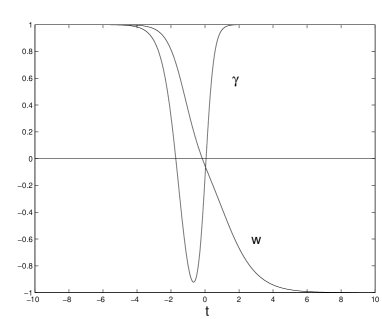
FIG. 1.: One-node solution monotonically interpolating between $1$ and $-1$ and the corresponding behavior of the negative friction coefficient $\gamma$

$n$	$\quad b$	$\quad M$
$1$	$\quad 1.27463\times 10^{1}\quad$	$1.13559$
2	$\quad 8.87397\times 10^{2}$	$\quad 1.21424$
3	$\quad 1.87079\times 10^{4}$	$\quad 1.23281$
4	$\quad 1.27455\times 10^{6}$	$\quad 1.23547$
5	$\quad 2.65030\times 10^{7}$	$\quad 1.23595$
6	$\quad 1.80475\times 10^{9}$	$\quad 1.23596$

Tab 1. Parameters $b,\,M$ for first six solutions.

This picture displays a striking similarity with the one occuring for the EYM system [7, 10]. However, there is one important distinction. In the EYM case the sequence $b_{n}$ converges to a finite value $b_{\infty}$, and the limiting solution exists with an infinite number of zeros [18]. In our case the sequence $b_{n}$ has no finite limit. The region of oscillations expands with growing $n$, and so does the size of the particles (see Fig. 2). Typically, the first and the last amplitude have large enough values, while in the middle zone the amplitude of oscillations becomes very small with increasing $n$ (i.e. an observer placed inside the core will see the unscreened magnetic charge). On the contrary, with $n$ increasing the mass rapidly converges to the finite value (9) corresponding to the abelian solution $w\equiv 0$.

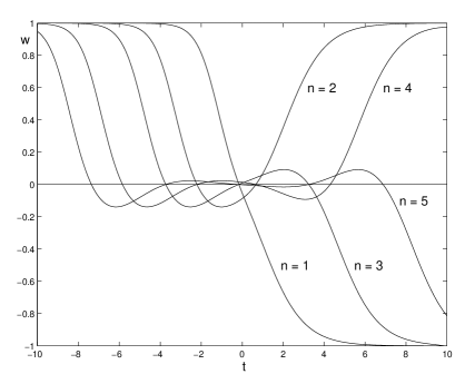
FIG. 2.: Solutions $w(\tau)$ for $n=1,...,5$.

Like in the BK case, solutions with odd and even node number $n$ have different physical meaning [10]. The lowest one with $n=1$ is the direct analog of the sphaleron. It can be shown to have the Chern-Simons number $Q=1/2$, to possess a fermionic zero mode and it is expected to have one odd-parity unstable decay mode along the path from the initial to the neighboring vacuum. The potential barrier between the neighboring vacua hence has a finite height. Higher odd-$n$ solutions also have $Q=1/2$, but possess more than one decay direction leading to the neighboring vacuum; they are expected to have $n$ odd-parity negative modes. Solutions with even values of $n$ have $Q=0$, and correspond to the paths in the phase space returning back to the same vacuum. These may be contiuously deformed to the trivial vacuum $w\equiv 1$ and therefore are topologically trivial.

If one uses the BIYM Lagrangian defined with the symmetrized trace, the equation of motion still preserves the form (7) with another friction coefficient $\gamma$ and an additional function of two variables ${\dot{w}}^{2},\,(1-w^{2})^{2}$ in front of the force term. It can be shown that the minima/maxima argument used above still holds as well as the $\gamma$-scaling argument. Therefore we expect that classical glueballs will persist in this version of the BIYM theory too.

It can be expected that the spectrum of magnetic monopoles in the BIYM–Higgs theory is affected by sphaleronic excitations like in the case of gauge monopoles coupled to gravity (for discussion and references see [10]). The occurence of the limiting value of $\beta$ found in [14] is likely to be a typical signal.

We wish to thank G.W. Gibbons, N.S. Manton, G. Clement and M.S. Volkov for valuable comments. One of the authors (DVG) would like to thank the Laboratory of Gravitation and Cosmology of the University Paris-6 for hospitality and the CNRS for support while this work was initiated.

REFERENCES

- [1] S. Deser, Phys. Lett., B 64, 463–464 (1976).
- [2] H. Pagels, Phys. Lett., B 68, 466–466 (1977).
- [3] S. Coleman. Comm. Math. Phys., 55, 113–116 (1977).
- [4] G.W.Gibbons, Lecture Notes in Phys., 383, 110-133. Springer-Verlag, Berlin, 1991.
- [5] R. F. Dashen, B. Hasslacher, and A. Neveu, Phys. Rev., D 10, 4138–4142 (1974).
- [6] N.S. Manton, Phys. Rev., D 28, 2019–2026 (1983).
- [7] R. Bartnik and J. McKinnon, Phys. Rev. Lett., 61, 141–144 (1988).
- [8] D.V. Gal’tsov and M.S. Volkov, Phys. Lett., B 273, 255–259 (1991).
- [9] D. Sudarsky and R.M. Wald, Phys. Rev., D 46, 1453–1447 (1992).
- [10] M.S. Volkov and D.V. Gal’tsov, Phys. Reports, C319, 1–83 (1999), hep-th/9810070.
- [11] A.Tseytlin, Nucl. Phys., B501 , 41 (1997).
- [12] J.P. Gauntlett, J. Gomis and P.K. Townsend, JHEP, 01, 003 (1998).
- [13] D. Brecher and M.J. Perry, Nucl. Phys., B527, 121 (1998).
- [14] N. Grandi, E.F. Moreno and F.A. Shaposhnik, Monopoles in non-Abelian Dirac-Born-Infeld theory, hep-th/9901073.
- [15] D.S. Chernavskii and R. Kerner, Journ. of Math. Phys., 9 (1), 287 (1978).
- [16] R. Kerner, Phys. Rev. D19 (4), 1243 (1979).
- [17] A.P. Protogenov, Phys. Lett, B87, 80 (1979).
- [18] P. Breitenlohner, P. Forgacs, and D. Maison, Comm. Math. Phys., 163, 141–172 (1994).