The Graceful Exit in Pre-Big Bang String Cosmology

Abstract:

We re-examine the graceful exit problem in the pre-Big Bang scenario of string cosmology, by considering the most general time-dependent classical correction to the Lagrangian with up to four derivatives. By including possible forms for quantum loop corrections we examine the allowed region of parameter space for the coupling constants which enable our solutions to link smoothly the two asymptotic low-energy branches of the pre-Big Bang scenario, and observe that these solutions can satisfy recently proposed entropic bounds on viable singularity free cosmologies.

1 Introduction

It is generally accepted that standard cosmology provides a consistent picture of the evolution of the Universe from the period of primordial nucleosynthesis to the present. However, as we extrapolate further into the past, our knowledge becomes less certain as we appear to be inevitably led to an initial curvature singularity [1]. The emergence of string theory as the favoured candidate to unify the forces of nature has led a number of authors to investigate the cosmology associated with it (for a recent review see [2]). One such approach has been pioneered by Veneziano and his collaborators, and employs the rich duality properties present in string theory [3, 4, 5, 6], and leads to a class of solutions which effectively talk about a period before the Big Bang, the pre-Big Bang scenario [6, 7]. The Universe expands from a weak coupling, low curvature regime in the infinite past, enters a period of inflation driven by the kinetic energy associated with the massless fields present, before approaching the strong coupling regime as the string scale is reached. There is then a branch change to a new class of solutions, corresponding to a post Big Bang decelerating Friedman-Robertson-Walker era. In such a scenario, the Universe appears to emerge because of the gravitational instability of the generic string vacua [8, 9]. In many ways this is a very appealing picture, the weak coupling, low curvature regime is a natural starting point to use the low energy string effective action. However, there are a number of problems facing the scenario. One is that of initial conditions, why should such a large Universe be a natural initial state to emerge from and does it possess enough inflation before entering the strong coupling regime [10, 11, 8]? The second is how can the dilaton field be stabilised in the post Big Bang phase? It must be decoupled from the expansion since variations in this scalar field correspond to changes in masses and coupling constants, which are strongly constrained by observation [12, 13]. A number of attempts have been made to do this; by including dilaton self-interaction potentials and trapping the dilaton in a potential minimum[14] and by taking into account the back-reaction on the dilaton field from quantum particle production [15]. The third is the graceful exit problem. How can the curvature singularity associated with the strong coupling regime be avoided, so as to allow a smooth branch change between the pre-Big Bang inflationary solution and a decelerating post Big Bang FRW solution? The simplest version of the evolution of the Universe in the pre-Big Bang scenario inevitably leads to a period characterised by an unbounded curvature. No-go theorems prevent the inclusion of a single potential to catalyse a graceful exit in vacuum-dilaton cosmology [16, 17, 18], although Ellis et al. recently claimed that non-singular evolutions can be obtained through the inclusion of a single scalar potential providing the use of an exotic equation of state [19]. The current philosophy is to include higher-order corrections to the string effective action. These include both classical finite size effects of the strings, and quantum string loop corrections and have already met with some success [20, 15, 21, 22]. The effect of backreaction arising from long wavelength modes, where string theory should be adequately described by general relativity with a minimally coupled scalar field, confirms that the qualitative effect of these corrections is compatible with an evolution leading towards exit [23].

The motivation behind this paper is to investigate the graceful exit issue by studying in detail a physically motivated action at both the classical and quantum level which can incorporate a number of appealing features, such as being able to maintain scale factor duality (SFD), even when these higher order corrections are included.

The classical corrections to the low energy effective string action usually have associated with them fixed points where the Hubble parameter in the string frame is constant and the dilaton is growing [20]. We will see that although physically very appealing, the SFD invariant action does not drive the evolution of the Universe into a good fixed point (in agreement with Brustein and Madden [24]), and moreover the inclusion of quantum corrections do not lead to a smooth exit into the decelerating FRW branch, rather they lead to a regime of instability. Fortunately, relaxing the SFD condition leads to many interesting features: the loop corrections introduce an upper (lower) bound for the curvature in the String (Einstein) frame, suggesting that a graceful exit is viable in this context, and indeed we present a number of successful exits.

The paper is organised as follows. In Section 2, we discuss the effective low energy action of the heterotic string including O($\alpha^{\prime}$) corrections arising from the finite size effects. In Section 3 we review previous studies of graceful exit using a truncated form of these corrections and then make a comparison with the full classical correction. A detailed analysis is presented showing the region of parameter space which admit classical fixed point solutions. We extend the analysis by including possible one- and two-loop quantum corrections. As expected these turn out to be important in order to obtain a successful graceful exit to the pre-Big Bang scenario [15, 24]. Particle creation is then used to stabilise the dilaton in the post-Big Bang era. Finally in Section 4 we summarise our main results.

2 String effective action

The pre-Big Bang scenario is an inflationary model starting with a generic state of extremely weak coupling and curvature, pictured as a gravitational collapse in the Einstein frame. This rather trivial asymptotic past state is followed by a dilaton-driven kinetic inflation phase which has to be long enough to solve the different cosmological problems inherent to standard cosmologies [8]. Later on, this superinflationary period should be smoothly connected to the FRW regime, characterised by a decelerating expansion and a frozen or slowly evolving dilaton, whose present expectation value gives rise to the universal gravitational constant.

We shall take as our starting point the minimal $4-$dimensional string effective action:

$$\Gamma^{(0)} = \frac{1}{\alpha^{\prime}}\int d^{4}x\sqrt{-g}{\cal L}^{(0)}$$ (1)

$$= \frac{1}{\alpha^{\prime}}\int d^{4}x\sqrt{-g}e^{-2\phi}\Bigl{\{}R+4(\partial_{\mu}\phi)^{2}\Bigr{\}},$$

where we adopt the convention $(-,+,+,+)$, $R^{\mu}_{\;\nu\lambda\rho}=\partial_{\rho}\Gamma^{\mu}_{\nu\lambda}+\dots$ and $R_{\nu\rho}=R^{\lambda}_{\;\nu\lambda\rho}$ and set our units such that $\hbar=c=16\pi G=1$. By low-energy tree-level effective action, we mean that the string is propagating in a background of small curvature and the fields are weakly coupled. However, the evolution from the pre-Big Bang era to the present is understood to be characterised by a regime of growing couplings and curvature. This means that the Universe will have to evolve through a phase when the field equations of this effective action are no longer valid. Hence, the low-energy dynamical description has to be supplemented by corrections in order to reliably describe the transition regime.

The finite size of the string will have an impact on the evolution of the scale factor when the curvature of the Universe reaches a critical level, corresponding to the string length scale $\lambda_{S}\sim\sqrt{\alpha^{\prime}}$ (fixed in the string frame), and such corrections are expected to stabilise the growth of the curvature into a de-Sitter like regime of constant curvature and linearly growing dilaton [20, 15]. Eventually the dilaton will play a major role, and since the loop expansion is governed by powers of the string coupling parameter $g_{S}=e^{\phi}$, these quantum corrections will modify dramatically the evolution when we reach the strong coupling region [15, 24]. This should correspond to the stage when the Universe completes a smooth transition to the post-Big Bang branch, characterised by a fixed value of the dilaton and a decelerating FRW expansion. One of the unresolved issues of the transition concerns whether or not the actual exit takes place at large coupling, $e^{\phi}\geq 1$. If it occurred whilst the coupling was still small, then we would be happy to use the perturbative corrections we are adopting. However, if the Universe is driven into the strong coupling regime before the exit proceeds then we might expect to have to adopt a different approach which involves the use of non-perturbative string phenomena. Such a possibility has recently been proposed in the context of M-theory [21, 25].

The type of corrections we will be considering involve truncations of the classical action at order $\alpha^{\prime}$. Although a field redefinition mixing the different orders in $\alpha^{\prime}$ does not change the physics if one considers all orders in $\alpha^{\prime}$, it inevitably leads to amBiguities when some orders are truncated. This means that the cosmological evolution arising from such actions truncated at order $\alpha^{\prime}$ should really only be considered as an indication of the possible cosmological behaviour. The most general form for a correction to the string action up to fourth-order in derivatives has been presented in refs [26, 27]:

$$\Gamma^{(C)} = \frac{1}{\alpha^{\prime}}\int d^{4}x\sqrt{-g}{\cal L}^{(C)}$$ (2)

$$= k\lambda_{0}\int d^{4}x\sqrt{-g}e^{-2\phi}\Bigl{\{}aR^{2}_{GB}+b\Box\phi(\partial_{\mu}\phi)^{2}$$

$$\hskip 102.43008pt+c\Bigl{\{}R^{\mu\nu}-\frac{1}{2}g^{\mu\nu}R\Bigr{\}}\partial_{\mu}\phi\partial_{\nu}\phi+d(\partial_{\mu}\phi)^{4}\Bigr{\}},$$

where the parameter $\lambda_{0}$ allows us to move between different string theories and we will set $k\lambda_{0}=-\frac{1}{4}$ to agree with previous studies of the Heterotic string [20]. $R^{2}_{GB}=R_{\mu\nu\lambda\rho}R^{\mu\nu\lambda\rho}-4R_{\mu\nu}R^{\mu\nu}+R^{2}$ is the Gauss-Bonnet combination which guarantees the absence of higher derivatives. In fixing the different parameters in this action we require that it reproduces the usual string scattering amplitudes [28]. This constrains the coefficient of $R_{\mu\nu\lambda\rho}^{2}$ with the result that the pre-factor for the Gauss-Bonnet term has to be $a=-1$. But the Lagrangian can still be shifted by field redefinitions which preserve the on-shell amplitudes, leaving the three remaining coefficients of the classical correction satisfying the constraint

$$2(b+c)+d=-16a.$$ (3)

There is as yet no definitive calculation of the full loop expansion of string theory. This is of course a Big problem if we want to try and include quantum effects in analysing the graceful exit issue. The best we can do, is to propose plausible terms that we hope are representative of the actual terms that will eventually make up the loop corrections. We believe that the string coupling $g_{S}$ actually controls the importance of string-loop corrections, so as a first approximation to the loop corrections we multiply each term of the classical correction by a suitable power of the string coupling [15]. When loop corrections are included, we then have an effective Lagrangian given by

$${\cal L}={\cal L}^{(0)}+{\cal L}^{(C)}+Ae^{2\phi}{\cal L}^{(C)}+Be^{4\phi}{\cal L}^{(C)},$$ (4)

where ${\cal L}^{(0)}$ is given in Eq. (1) and ${\cal L}^{(C)}$ given in Eq. (2). The constant parameters $A$ and $B$ actually control the onset of the loop corrections.

3 Numerical solutions

In this section, we consider the impact of both the classical and quantum corrections of Eq. (4). Naively, we would expect that the latter should only become significant as we enter the strong coupling regime. Depending on the value of the dilaton field, the loop corrections are indeed negligible in the weak coupling regime as the dilaton $\phi\rightarrow-\infty$, so we expect that the solutions to the extended equations of motion should initially be similar to the lowest-order description, with the classical and quantum corrections introducing an upper bound for the solutions, thereby regulating their singular behaviour.

Following Brustein and Madden [15], we define the parameters $H_{S}$ as the Hubble expansion in the string frame, $H_{E}$ as the Hubble expansion in the Einstein frame and $\dot{\phi}$ the derivative of the dilaton field with respect to cosmic time, $t_{S}$. Hence, the solutions to the equations of motion resulting from Eq. (1) can be expressed as $2\dot{\phi}=(3\pm\sqrt{3})H_{S}$, where the upper (lower) sign refers to the pre- (post-) Big Bang solution. Although starting in the perturbative regime, the $(+)$ branch ($H_{S}>0$, $\dot{\phi}>0$ and $H_{E}<0$) evolves toward a curvature singularity, and the low-energy effective description breaks down. More precisely, we expect modifications to become significant when the curvature is of order the Planck length $\lambda_{S}$ and the low-energy effective action has to be replaced by one which includes higher-order effects in $\alpha^{\prime}$. It has been known for some time that such classical corrections allow a branch change $(+)\rightarrow(-)$, which corresponds to a change of sign of the shifted dilaton, $\dot{\bar{\phi}}\equiv\dot{\phi}-3H_{S}/2$ [29]. Also, to allow a smooth connection to the usual decelerated Friedmann Universe where the dilaton will become fixed, the Hubble rate in the Einstein frame has to become positive after the branch change. Using the conformal transformation relating the String frame to the Einstein frame, $g^{E}_{\mu\nu}=e^{-2\phi}g^{S}_{\mu\nu}$, the Hubble expansion in the E-frame can be expressed as a function of S-frame quantities, $H_{E}=e^{\phi}\{H_{S}-\dot{\phi}\}$. This relation allows us to define the Einstein bounce $E_{B}=H_{S}-\dot{\phi}=0$. A necessary condition to obtain a successful exit is the violation of the null energy condition (NEC) in the Einstein frame, which is associated with the cross over of the Einstein bounce[29]. Thus we see that a number of different conditions must be satisfied for a successful exit to be obtained. In the figures below, all these constraints are presented as lines on the plots, i.e. the $(+)$ and $(-)$ branches of the low energy string action, the branch change and the Einstein bounce.

3.1 Classical correction

We first recall some aspects of the background evolution when we restrict ourselves to the classical corrections. Choosing initial conditions on the pre-Big Bang branch, the equations of motion derived from Eq. (1) and Eq. (2) lead in general to a regime of constant Hubble parameter $H$ and a linearly growing dilaton $\dot{\phi}>0$. This is quantified in figure 1, where we show the different types of solutions that can be found in the $(c,d)$ plane, when we choose $a=-1$ and determine $b$ from the constraint Eq. (3). The distribution of red dots corresponds to values of $(c,d)$ which lead to standard fixed point solutions, $H={\rm const},~{}\dot{\phi}>0$. The set of blue points (which starts approximatively for $c\geq 12$) also shows coefficients leading to a fixed point, but with a Hubble parameter, $H\geq 1$. In particular we see that these points are bordered by the lines $d\geq 1.68c+3.62$ and $c\leq 152/9$, indicating that these represent the constraints on $c$ and $d$ which have to be satisfied in order to obtain satisfactory fixed point solutions. It is clear that there exists a large region of parameter space where such solutions are to be found. Representing these fixed points in the $(2\dot{\bar{\phi}},H)$ plane emphasizes that for a constant $c=0$ the fixed point moves to smaller values of $|\dot{\bar{\phi}}|$ and $H$ when we increase the coefficient $d$ (green curve), whereas $|\dot{\bar{\phi}}|$ and $H$ both become larger when we increase $c$ keeping constant $d=16$ (blue curve). This latter curve corresponds to a segment of the more general case $b=-c$ where the asymptotic state in the high curvature regime is given by the implicit equation:

$$0 = -\frac{3}{16}H(2\dot{\bar{\phi}}+3H)\Bigl{\{}63\dot{\bar{\phi}}H^{5}+126\dot{\bar{\phi}}^{2}H^{4}-18H^{4}+8\dot{\bar{\phi}}^{3}H^{3}-96\dot{\bar{\phi}}H^{3}$$

$$\hskip 96.73918pt-176\dot{\bar{\phi}}^{4}H^{2}-144\dot{\bar{\phi}}^{2}H^{2}-144H\dot{\bar{\phi}}^{5}-128\dot{\bar{\phi}}^{3}H-32\dot{\bar{\phi}}^{6}-32\dot{\bar{\phi}}^{4}\Bigr{\}}.$$

However, we will see later in the analysis that not all values of this curve of fixed points can be reached if the initial conditions are chosen on the pre-Big Bang branch.

The region to the right of the black line $d\leq 4c-44.62$ in figure 1, represents the range of coefficients which lead to an evolution heading away from the $\dot{\bar{\phi}}\leq 0$ region. The line was first proposed by [24]. Finally, the intermediate blank area represents the combination of parameters driving the evolution into a regime of instability for the scale factor, where $\ddot{a}\rightarrow\infty$. The emergence of such a region requires further investigation.

We now go on to look at some particular examples including quantum loop corrections.

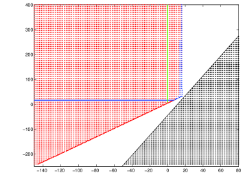
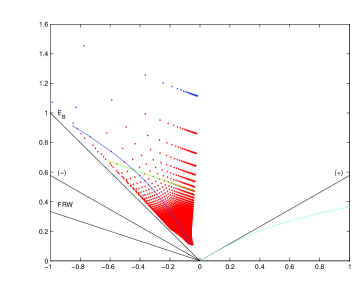
Figure 1: On the left, we have represented in the $(c,d)$ plane the asymptotic state of the evolution when the classical corrections are included, with $a=-1$ and the remaining parameter $b$ is constrained by Eq. (3). The red dots show the combinations of these parameters leading to a fixed point, with saturated Hubble parameter $H={\rm const}$ and a linearly growing dilaton. The black points indicate the set of coefficients forcing the evolution to head away from the $\dot{\bar{\phi}}\leq 0$ region. The black line represents the bound given in [24]. The figure on the right shows the fixed point distribution in the plane $(2\dot{\bar{\phi}},H)$. The green line corresponds to a constant $c=0$, whereas the red line stands for $d=16$. The cyan line shows the evolution for the SFD case with $c=4$ and $d=16$: the curve heads away from the $\dot{\bar{\phi}}\leq 0$ region, typical of the black dots area in the figure on the left.

3.2 Minimal case

The natural setting $b=c=0$ leads to the well-known form which has given rise to most of the studies on corrections to the low-energy picture. In references [20, 15], the authors demonstrated that this minimal classical correction regularises the singular behaviour of the low-energy pre-Big Bang scenario. It drives the evolution to a fixed point of bounded curvature with a linearly growing dilaton (the star in figure 2 – which agrees with the results of [20, 15]), suggesting that quantum loop corrections -known to allow a violation of the null energy condition $(p+\rho<0)$- would permit the crossing of the Einstein bounce to the FRW decelerated expansion in the post-Big Bang era. Indeed, the addition of loop corrections leads to a $(-)$ FRW-branch as pictured in figure 2. However, we still have to freeze the growth of the dilaton. Following [15], we introduce by hand a particle creation term of the form $\Gamma_{\phi}\dot{\phi}$, where $\Gamma_{\phi}$ is the decay width of the $\phi$ particle, in the equation of motion of the dilaton field and then coupling it to a fluid with the equation of state of radiation in such a way as to preserve overall conservation. This allows us to stabilise the dilaton in the post-Big Bang era with a decreasing Hubble rate, similar to the usual radiation dominated FRW cosmology.

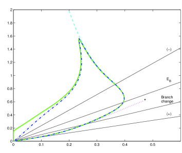
Figure 2: Hubble expansion in the S-frame as a function of the dilaton for the case $a=-1$, $b=c=0$ and $d=16$. The y-axis corresponds to $H$, and the x-axis to $2\dot{\phi}/3$. The initial conditions for the simulations have been set with respect to the lowest-order analytical solutions at $t_{S}=-1000$. The straight black lines describe the bounds quoted in Section II. The dotted magenta line shows the impact of the classical correction due to the finite size of the string. A $*$ denotes the fixed point. The contribution of the one-loop expansion is traced with a dashed cyan line ($A=4$). The dash-dotted blue line represents the incorporation of the two-loop correction without the Gauss-Bonnet combination ($B=-0.1$). Finally, the green plain line introduces radiation with $\Gamma_{\phi}=0.08$ and stabilises the dilaton.

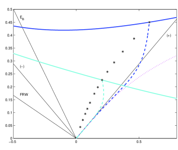
Figure 3: Hubble expansion in the S-frame as a function of the shifted dilaton $(2\dot{\bar{\phi}})$ for the SFD case, with $a=-1$, $b=-c=-16$ and $d=16$. Straight lines are identical to those in figure 2. The classical correction makes the curve turn the wrong way (dotted magenta). The inclusion of the one-loop correction (dashed) leads to a regime of instability: the evolution meets the curve corresponding to $\ddot{a}\rightarrow\infty$ (plain). Two cases are explicitly shown: $A=0.5$ in blue and $A=16$ in cyan, whereas the meeting points for other choices of the pre-factor $A$ are pictured with stars (*).

3.3 Scale factor duality case

In [26, 27], the authors considered the particular combination $b=-c=-16$ which has the remarkable property of introducing scale factor duality at the order $\alpha^{\prime}$ in the correction to the low-energy action at the price of discarding non-SFD invariant terms of higher order and making a modification to the definition of SFD at order $\alpha^{\prime}$. Unfortunately, as can be seen in figure 3, this choice of parameters does not lead to a successful exit. The classical correction forces the curve to head away from the branch changing and exit region. In fact even including loop corrections it is impossible to reach the branch change, given in figure 3 by the line $\dot{\bar{\phi}}=0$. Such an observation was previously also made in [24]. What appears to be happening is that including the one-loop correction drives the system into a regime where the acceleration of the scale factor $(\ddot{a})$ diverges. This is a singular point in the equation of motion and is indicated by the star in figure 3. As discussed in [24], it may be that working with higher orders in the corrections requires further alterations of the form of SFD.

3.4 The general case

Relaxing the SFD constraint allows us to investigate the full classical and quantum correction up to four derivatives and leads to many interesting situations. When $a=-1$ and $d=16$, this implies that the coefficient of the curvature-dilaton contribution has the opposite sign to that of the $\Box\phi(\partial_{\mu}\phi)^{2}$ term. Figure 4 shows the evolution of the solution for $b=-c=-4$. The fixed point obtained by adding classical corrections to the lowest-order action is well located as the evolution has already reached the $\dot{\bar{\phi}}\leq 0$ region of the $(H,\dot{\bar{\phi}})$ phase space, indicating that generic loop corrections will drive the evolution across the Einstein bounce. Indeed, setting $A=+4$ we see that the evolution crosses the Einstein bounce as well as the $(-)$ branch. This suggests that the violation of the NEC is too large and will not give an upper bound to the curvature in the Einstein frame. An extra two-loop term is thus required to instigate the transition to a decelerated expansion in the Einstein frame. As shown in figure 4 when such a term is included with $B=-0.3$, we obtain a successful implementation of the graceful exit. Once again, we invoke particle production in order to eventually stabilise the dilaton in the usual FRW cosmology.

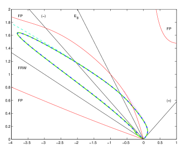
Figure 4: Hubble expansion in the S-frame as a function of the shifted dilaton $(2\dot{\bar{\phi}})$ for the case $a=-1$, $b=-c=-4$ and $d=16$, with $A=+4$ (dashed cyan) and $B=-0.3$ (dash-dotted blue). The plain green line includes the effect of the particle creation, with $\Gamma_{\phi}=0.2$. The FRW and FP lines represent solutions for the fixed points given in Eq. (3.1).

An important issue concerns the sensitivity of our results to the values of the parameters $a,b,c,d,A$ and $B$. Do we find successful transitions for only a small range of these values, in which case we should be concerned that our solutions are not representative of the typical case? Fortunately, we have established that there does exist a large range of values of the parameters which allow for successful exits between the two branches. Figure 1 shows the range that lead to fixed point solutions when just the classical corrections are included. From such a solution, it is then relatively straightforward to achieve a successful exit through the addition of the quantum corrections.

The role of $A$ and $B$ is less clear cut. Their actual values determine the onset when loop corrections become important, hence the value of $\phi$ when the graceful exit is successfully completed. Generally we find that a successful exit requires $A>0$ and $B<0$, implying that the two quantum loop terms compete against each other in order to lead to a successful exit. Unfortunately there is a degree of amBiguity present which arises because of the invariance of the system of equations under a constant shift of $\phi\to\phi+{\rm const}$, with a compensating shift of $A$ and $B$. The invariance of the system (up to a multiplicative constant in the action) is manifest at the tree level and implies that we can make $\phi$ arbitarily negative and guarantees a transition in the weak coupling regime. As mentioned earlier, when the loop corrections are included, this simple invariance is broken and the shift in $\phi$ is compensated for by a shift in $A$ and $B$. For example, if we take the case $b=-c=-4$ and set $A=+4$ and $B=-0.3$, we obtain a graceful exit with $\phi_{final}\simeq 0.75$. In shifting the dilaton by $\phi_{*}=-1.5$, the equivalent dynamical evolution is obtained with a final value $\phi_{final}\simeq-0.65$ (weak coupling) with $A\to e^{2\phi_{*}}A=80.34$ and $B\to e^{4\phi_{*}}B=-121.03$. There appears to be a price to pay, weak coupling seems to imply large loop coefficicents. Normally we would expect the coefficients of successive loops to be less important. This behaviour raises an interesting question as to whether it is possible to have genuinely weak coupling transitions with just loop corrections included. We have tried this for a wide range of the fixed point solutions and found the same type of behaviour.

3.5 Entropic bounds

There has recently been considerable interest in the possibility that entropy considerations can provide new constraints on the allowed evolution of the Universe [30, 31, 32, 33]. Veneziano has suggested that in the context of string cosmology, non-singular cosmologies should respect at all times a Hubble entropy bound [31]. Brustein has proposed that such solutions should satisfy a slightly different bound arising from a generalised second law of thermodynamics (GSL) [32]. Do our non-singular solutions satisfy these bounds?

We will concentrate on the example of the Hubble entropy bound [31]. Following Bekenstein’s work [34], Veneziano suggested that for a homogeneous cosmology, the radius of the largest black hole that can form is determined by the largest causal scale available, namely the Hubble radius $H^{-1}$. The maximum entropy enclosed in such a Universe corresponds to having one black hole in a Hubble volume. Defining $n_{H}=a^{3}H^{3}$ to be the number of cosmological horizons within a given comoving volume and $S_{H}=|H|^{-2}e^{-2\phi}$ the maximal entropy within the horizon corresponding to a black hole of radius $H^{-1}$, the Hubble entropy is given by $S_{HB}=a^{3}He^{-2\phi}$ [31]. From this it follows that:

$$\partial_{t}\;S_{HB}=n_{H}\partial_{t}S_{H}+S_{H}\partial_{t}n_{H}.$$ (6)

Enforcing that the rate of change of this geometric entropy $\partial_{t}\;S_{HB}\geq 0$ leads to the reduced inequality

$$\frac{\dot{H}}{H}-2\dot{\bar{\phi}}\geq 0$$ (7)

with the lowest-order solutions of the PBB scenario saturating this geometric bound [31, 35, 36]. Furthermore, it indicates that a fixed point necessarily occurs for non-positive $\dot{\bar{\phi}}$ (a conclusion that also follows from the presence of a conserved quantity in the solutions [20]). Brustein et al. provided evidence in [33] that the bound was satisfied for the non-singular solutions arising out of the purely classical correction Eq. (2) satisfying $a=-1$ and the constraint Eq. (3). We have confirmed this result, although we have also found that all the non-singular solutions we have obtained, when including loop corrections, lead to violations of this bound over short time intervals. However, as pointed out by Veneziano, this is really a global bound, in the asymptotic future, as we enter the FRW phase, we always find that $S_{HB}$ has increased. An example of this can be seen in figure 5.

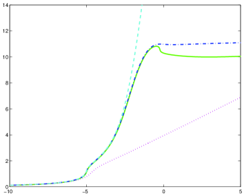
Figure 5: $ln(S_{HB})_{t_{final}}-ln(S_{HB})_{t_{initial}}$ plotted as a function of $t_{final}$ for the setting $a=-1$, $b=-c=-4$ and $d=16$. The dotted line represents the classical correction, then the loop corrections with $A=+4$ (dashed line) and $B=-0.3$ (dash-dotted line). The plain green line also includes the effect of particle creation, with $\Gamma_{\phi}=0.2$.

The comparison becomes a bit more difficult when considering the bound proposed by Brustein arising from a generalised second law of thermodynamics (GSL) [32]. We do find a class of solutions which satisfy such a bound for positive values of the chemical potential $\mu$ that he introduced, but we also find solutions which violate the bound. It is difficult to draw any real conclusion from this, not least because we do not know the precise form of the quantum corrections or particle production the true graceful exit solution will contain. It is certainly interesting that there are regions of parameter space where the bound is satisfied. The nature of these bounds is also under active consideration at the moment [37].

4 Conclusions

In this paper, we have obtained a class of non-singular cosmologies, based on an effective action given in Eqs. (1), (2) and (4). The inclusion of such classical and quantum corrections can lead to an evolution which smoothly joins the inflationary pre-Big Bang solution with a decelerating FRW universe. The classical correction is based on an enhanced form of the action which includes up to four derivatives in the fields. The importance of quantum loops in achieving a smooth transition has become manifest, in agreement with [15, 24]. Furthermore, we observe that these non-singular solutions can satisfy the recently proposed entropics bounds when loop-corrections are included.

Although encouraging, the solutions we have presented still have side effects; in particular we had to stabilise the dilaton by hand. Also, it proved quite difficult to obtain the transition in the weak coupling regime, whilst keeping the loop corrections small. It is not clear to us, how serious an issue this is as we do not know the form of the true corrections. An intriguing issue is the unusual behaviour surrounding the SFD case. Why do these singular regions arise and what do they correspond to physically?

Finally, we would like to comment on a possible natural extension of this work. Recently in refs [38, 39] the authors have developed a technique to determine the large-scale CMB anisotropy and power spectra generated by massless axionic seeds in the pre-Big Bang scenario. They numerically determined the CMB anisotropy power spectrum and pointed out the differences (’isocurvature hump’ at $l\sim 40$ and first acoustic peak at $l\sim 300$) with more standard adiabatic models. These are fascinating results, but are based on numerical solutions for the curvature and dilaton that have not really avoided the curvature singularity. Instead they are frozen at some scale, and then begin evolving again once the post Big Bang FRW branch is entered. We are in a position to provide solutions where the background fields evolve right through the transition in a singularity free manner, and it would be useful to determine how such an evolution impacts on the modes leaving the horizon during the transition period. How (if at all) do they influence the CMB spectrum at large $l$? This is currently under investigation.

- [1] S.W. Hawking and R. Penrose, Proc. Roy. Soc. Lond. A 314 (1979) 529.
- [2] J.E. Lidsey, D. Wands and E.J. Copeland, hep-th/9909061.
- [3] R. Brandenberger and C. Vafa, Nucl. Phys. B 316 (1989) 391.
- [4] G. Veneziano, Phys. Lett. B 265 (1991) 287.
- [5] A. A. Tseytlin and C. Vafa, Nucl. Phys. B 372 (1992) 443.
- [6] M. Gasperini and G.Veneziano, Astropart. Phys. 1 (1993) 317; Mod. Phys. Lett. A 8 (1993) 3701; Phys. Rev. D 50 (1994) 2519.
- [7] An updated collection of papers and references on the pre-Big Bang scenario is available at ”http://www.to.infn.it/teorici/gasperini/”
- [8] A. Buonanno, T. Damour and G. Veneziano, Nucl. Phys. B 543 (1999) 275.
- [9] M. Gasperini, gr-qc/9902060.
- [10] M. S. Turner and E. J. Weinberg, Phys. Rev. D 56 (1997) 4604.
- [11] N. Kaloper, A. D. Linde, and R. Bousso, Phys. Rev. D 59 (1999) 043508.
- [12] T. Damour and A.M. Polyakov, Nucl. Phys. B 423 (1994) 532.
- [13] B.A. Campbell and K.A. Olive, Phys. Lett. B 345 (1995) 429.
- [14] T. Barreiro, B. de Carlos and E. J. Copeland, Phys. Rev. D 58 (1998) 083513.
- [15] R. Brustein and R. Madden, Phys. Rev. D 57 (1998) 712.
- [16] R. Brustein and G. Veneziano, Phys. Lett. B 329 (1994) 429.
- [17] N. Kaloper, R. Madden and K. A. Olive, Nucl. Phys. B 452 (1995) 677.
- [18] N. Kaloper, R. Madden and K. A. Olive, Phys. Lett. B 371 (1996) 34.
- [19] G.F.R. Ellis, D.C. Roberts, D. Solomons and P.K.S. Dunsby, gr-qc/9912005.
- [20] M. Gasperini, M. Maggiore and G. Veneziano, Nucl. Phys. B 494 (1997) 315.
- [21] S. Foffa, M. Maggiore and R. Sturani, Nucl. Phys. B 552 (1999) 395.
- [22] I. Antoniadis, J. Rizos and K. Tamvakis, Nucl. Phys. B 415 (1994) 497; R.H. Brandenberger, R. Easther and J. Maia, J. High Energy Phys. 08 (1998) 007; D.A. Easson and R.H. Brandenberger, J. High Energy Phys. 09 (1999) 003.
- [23] A. Ghosh, R. Madden and G. Veneziano, hep-th/9908024.
- [24] R. Brustein and R. Madden, J. High Energy Phys. 07 (1999) 006.
- [25] M. Maggiore and A. Riotto, Nucl. Phys. B 548 (1999) 427.
- [26] K.A. Meissner, Phys. Lett. B 392 (1997) 298.
- [27] N. Kaloper and K.A. Meissner, Phys. Rev. D 56 (1997) 7940.
- [28] R.R. Metsaev and A.A. Tseytlin, Nucl. Phys. B 293 (1987) 385.
- [29] R. Brustein and R. Madden, Phys. Lett. B 410 (1997) 110.
- [30] R. Easther and D. Lowe, Phys. Rev. Lett. 82 (1999) 4967.
- [31] G. Veneziano, Phys. Lett. B 454 (1999) 22.
- [32] R. Brustein, gr-qc/9904061.
- [33] R. Brustein, S. Foffa and R. Sturani, hep-th/9907032.
- [34] J.D. Bekenstein, Phys. Rev. D 23 (1981) 287.
- [35] D. Bak and J.S. Rey, hep-th/9902173.
- [36] N. Kaloper and A. Linde, Phys. Rev. D 60 (1999) 103509.
- [37] R. Brustein and G. Veneziano, hep-th/9912055.
- [38] R. Durrer, M. Gasperini, M. Sakellariadou and G. Veneziano, Phys. Rev. D 59 (1999) 043511.
- [39] A. Melchiorri, F. Vernizzi, R. Durrer and G. Veneziano, Phys. Rev. Lett. 83 (1999) 4464.