DPT/99/73

Microscopic- versus Effective Coupling in N=2 Yang-Mills With Four Flavours
Ivo Sachs and William Weir

Department of Mathematical Sciences
University of Durham
Science Site, Durham DH1 3LE, UK

We determine the instanton corrections to the effective coupling in $SU(2)$, $N\!=\!2$ Yang-Mills theory with four flavours to all orders. Our analysis uses the $S(2,Z)$-invariant curve and the two instanton contribution obtained earlier to fix the higher order contributions uniquely.

1 Introduction

Seiberg and Witten [1, 2] proposed exact results for $SU(2)$, $N\!=\!2$ supersymmetric Yang-Mills theory with and without matter multiplets. These include, in particular an exact expression for the mass spectrum of BPS-states for these theories. Their solutions also provide a mechanism, based on monopole condensation, for chiral symmetry breaking and confinement in $N\!=\!2$ Yang-Mills with and without coupling to fundamental hypermultiplets respectively. The results of Seiberg and Witten have since been generalised to a variety of gauge groups [3] describing a number of interesting new phenomena [4].

On another front the low energy effective theories arising from non-Abelian YM-theory have been identified with those describing the low energy dynamics of certain intersecting brane configurations in string theory [5]. This approach to field theory has the advantage of providing an elegant geometrical representation of the low energy dynamics of strongly coupled supersymmetric gauge theory.

For gauge groups $SU(2)$ and $N_{F}\leq 3$ massless flavours it has since been shown that the solution [1, 2] are indeed the only ones compatible with supersymmetry and asymptotic freedom in these theories [6]. However, a number of issues have still resisted an exact treatment. In particular the precise relation between the low energy effective coupling $\tau_{\hbox{\tiny eff}}$ and the microscopic coupling $\tau$ in the scale invariant $N_{F}\!=\!4$ theory has not been understood so far. Indeed, while the two couplings were first assumed to be identical in [2] it was later found by explicit computation that there are, in fact, perturbative as well as instanton corrections [7]. On the other hand, explicit instanton calculus is so far limited to topological charge $k\leq 2$. A related observation has been made in the D-brane approach to scale invariant theories. The details of the conclusions reached there are, however, somewhat different [8].

The purpose of the present paper is to fill this gap. Our analysis uses a combination of analytic results from the theory of conformal mappings combined with the known results form instanton calculus. More precisely we consider the sequence $\tau\mapsto z\in{\bf C}\mapsto\tau_{\hbox{\tiny eff}}$. We will then argue that given the Seiberg-Witten curve together with some suitable assumptions on the singular behaviour of the instanton contributions there is a one-parameter family of admissible maps $\tau_{\hbox{\tiny eff}}\mapsto\tau$. The remaining free parameter is in turn determined by the two-instanton contribution to the asymptotic expansion at weak coupling. This coefficient has been computed explicitly in [7]. Combining these results then determines the map completely. Although we are not able to give a closed form of the map $\tau\mapsto\tau_{\hbox{\tiny eff}}$ globally the higher order instanton coefficients can be determined iteratively. We further discuss some global properties of the map qualitatively. In particular we will see that it is not single valued meaning that the instanton corrections lead to a cut in the strong coupling regime. In this note we restrict ourselves to gauge group $SU(2)$ leaving the extension to higher groups [9] for future work.

2 Review of N=2 Yang-Mills with 4 Flavours

To prepare the ground let us first review some of the relevant features of the theory of interest [2], that is $N\!=\!2$ YM-theory with $4$ hypermultiplets $Q^{r}$ and $\tilde{Q}_{r}$, $r\!=\!1,\cdots,4$, in the fundamental representation. In $N\!=\!1$ language the hypermultiplets are described by two chiral multiplets containing the left handed quarks and anti quarks respectively. These are in isomorphic representations of the gauge group $SU(2)$. The global symmetry group therefore contains a $SO(8)$ or, more precisely, a $O(8)$ due to invariance under the ${\bf Z}_{2}$ “parity” which exchanges a left handed quark with its anti particle, $Q_{1}\leftrightarrow\tilde{Q}_{1}$, with all other fields invariant. At the quantum level this ${\bf Z}_{2}$ is anomalous due to contributions from odd instantons.

We consider the Coulomb branch with a constant scalar $\varphi\!=\!a\neq 0$ in the $N\!=\!2$ vector multiplet. This breaks the gauge group $SU(2)\to U(1)$. The charged hypermultiplets then have mass $M\!=\!\sqrt{2}|a|$ and transform as a vector under $SO(8)$, rather than $O(8)$ due to the ${\bf Z}_{2}$-anomaly. In addition, there are magnetic monopole solutions leading to $8$ fermionic zero modes from the $4$ hypermultiplets. These turn the monopoles into spinors of $SO(8)$. The symmetry group is therefore the universal cover of $SO(8)$ or Spin$(8)$ with centre ${\bf Z}_{2}\times{\bf Z}_{2}$. Following [2] we label the representations ${\bf Z}_{2}\times{\bf Z}_{2}$ according to the Spin$(8)$ representations, that is the trivial representation $o$, the vector representation $v$ and the two spinor representations $s$ and $c$. To decide in which spinor representation the monopoles and dyons transform one considers the action of an electric charge rotation $e^{\pi iQ}$ on these states. Here the electric charge $Q$ is normalised such that the massive gauge bosons have charge $\pm 2$. This action is conveniently described by

$$e^{\pi iQ}=e^{{in_{m}\theta}}(-1)^{H},$$ (1)

where states with even, odd $n_{e}$ are $(-1)^{H}$ even, odd respectively. On the other hand, for consistency, the monopole anti-monopole annihilation process requires a correlation between chirality in Spin$(8)$ and electric charge [2]. We therefore identify $(-1)^{H}$ with the chirality operator in the spinor representations of Spin$(8)$. Hence dyons with even and odd electric charge transform in one or the other spinor representation of Spin$(8)$ respectively. There is an outer automorphism $S_{3}$ of Spin$(8)$ that permutes the three non-trivial representations $v$, $s$ and $c$. It is closely connected to the proposed duality group $SL(2,{\bf Z})$ of the quantum theory. Indeed there is a homomorphism $SL(2,{\bf Z})\to S_{3}$, so that the invariance group of the spectrum is given by the semi direct product Spin$(8)$ and $SL(2,{\bf Z})$. The kernel of this homomorphism plays an important part in our analysis below. It consists of the matrices congruent to $1$ (mod$(2)$). They are conjugate to the subgroup $\Gamma_{0}(2)$. The fundamental domain of this subgroup is the space of inequivalent effective couplings $\tau_{\hbox{\tiny eff}}$.

One can further formalise this structure in terms of the hyperelliptic curve that controls the low energy behaviour of the model [2]. For this one seeks a curve $y^{2}\!=\!F(x,u,\tau)$ such that the differential form

$$\omega=\frac{\sqrt{2}}{8\pi}\frac{\hbox{d}x}{y}$$ (2)

has the periods $(\frac{\partial a_{D}}{\partial u},\frac{\partial a}{\partial u})$ with $(a_{D},a)$ given by [2]

$$a=\sqrt{\frac{u}{2}}\quad\hbox{{and}}\quad a_{D}=\tau_{\hbox{\tiny eff}}a.$$ (3)

The curve consistent with $SL(2,{\bf Z})$ duality determined in [2], is given by

$$y^{2}=(x-ue_{1}(\tau))(x-ue_{2}(\tau))(x-ue_{2}(\tau)),$$ (4)

where $e_{i}(\tau)$ are the modular forms corresponding to the three subgroups of $SL(2,{\bf Z})$, conjugate to the index $3$ subgroup $\Gamma_{0}(2)$.

3 Map: $\tau\mapsto\tau_{\hbox{\tiny eff}}$

We now have the necessary ingredients to determine the precise relation between $\tau_{\hbox{\tiny eff}}$ and $\tau$. We begin with the observation that, according to the structure of the effective theory presented above, the fundamental domain $D_{\Gamma}$ of any of the three subgroups conjugate to $\Gamma_{0}(2)$ can be used as the space of inequivalent effective couplings. The three choices are then related by the Spin$(8)$ “triality” relating the $3$ different non-trivial representations $v$, $s$ and $c$. Each fundamental domain is described by a triangle in the upper half plane ($\hbox{Im}(\tau)\geq 0$), bounded by circular arcs [10]. The $3$ singularities are conjugate to the points $(i\infty,-1,1)$ corresponding to the weak coupling regime, massless monopoles and massless dyons with charge $(n_{m},n_{e})\!=\!(1,1)$ mod$(2)$ respectively.

In the absence of perturbative- and instanton corrections the effective coupling is identified with the microscopic coupling $\tau$. This is the case in $N\!=\!4$ theories. In the scale invariant $N\!=\!2$ theory considered here the situation is different. As shown in [7], the effective coupling is finitely renormalised at the one loop level and furthermore receives instanton corrections. As a result the fundamental domain $\bar{D}$, of inequivalent microscopic couplings and the fundamental domain $D_{\Gamma}$, of inequivalent effective couplings are not the same. We will now determine the exact relation between them.

Some information about the fundamental domain $\bar{D}$ of microscopic couplings $\tau$ is obtained from the following observations: a)   As the microscopic coupling does not enter in the mass formula, its fundamental domain is not constrained to be that of a subgroup of $SL(2,{\bf Z})$ [6]. Nevertheless we require that the imaginary part of $\tau$ be bounded from below. Correspondingly the different determinations of $\tau$ for a given $\tau_{\hbox{\tiny eff}}$ must be related by a transformation in $G\subset PSL(2,{\rm I\!R})$. Hence, a particular determination of $\tau$. will lie within a fundamental domain of $G$ or some covering thereof. That is,

$$\tau\in C[H/G]\quad\hbox{{where}}\quad G\subset PSL(2,{\rm I\!R}),$$ (5)

where $C[\;]$ denotes a certain covering. Any such domain is bounded by circular arcs and is thus conformally equivalent to the punctured $2$-sphere, ${\bf C}-\{a_{1},\cdots,a_{n}\}$ [10]. b)   We know of no principle excluding the possibility that the number of vertices of $\bar{D}$ be different from that of $D_{\Gamma}$. On the other hand such extra singularities have no obvious physical interpretation. We therefore discard this possibility.

Equipped with this information we will now determine the homomorphism that maps $D_{\Gamma}$ into the fundamental domain of microscopic couplings $\bar{D}$. It follows from general arguments [2, 7] that this map has an expansion of the form

$$\tau_{\hbox{\tiny eff}}=\sum\limits_{n=0}^{\infty}c_{n}q^{n}\quad\hbox{{where}}\quad q=e^{\pi i\tau}$$ (6)

The coefficients $c_{i}$, represent the perturbative one-loop ($i\!=\!0$) and instanton ($i\!>\!0$) corrections respectively. The contributions from odd instantons to $\tau_{\hbox{\tiny eff}}$ vanishes. This is due the fact that the part of the effective action determining the effective coupling is invariant under the ${\bf Z}_{2}$-”parity” described in the last section. The first two non-vanishing coefficients of the expansion (6) are known [7]. They are

$$c_{0}=\frac{i}{\pi}4\ln 2\quad\hbox{{and}}\quad c_{2}=-\frac{i}{\pi}\frac{7}{2^{5}\cdot 3^{6}}.$$ (7)

To continue we use some elements of the theory of conformal mappings [10]. That is we consider the maps from the punctured $2$-sphere $S={\bf C}-\{a_{1},\cdots,a_{n}\}$ to polygons in the upper half plane, bounded by circular arcs. Concretely we consider the sequence $\tau_{\hbox{\tiny eff}}\mapsto z\in S\mapsto\tau$ (see Fig.1). The form of such mappings is generally complicated. However, their Schwarzian derivative takes a remarkably simple form [10]

$$\{\tau,z\}=\sum\limits_{i}{1\over 2}\frac{1-\alpha_{i}^{2}}{(z-a_{i})^{2}}+\frac{\beta_{i}}{z-a_{i}}.$$ (8)

The parameters $\alpha_{i}$ measure the angles of the polygon in units of $\pi$. The accessory parameters $\beta_{i}$ do not have a simple geometric interpretation but are determined uniquely up to a $SL(2,{\bf C})$ transformation of $S$. Furthermore they satisfy the conditions [10]

$$\sum_{i=1}^{n}\beta_{i}=0 \sum_{i=1}^{n}\left[2a_{i}\beta_{i}+1-\alpha_{i}^{2}\right]=0,$$ ,

$$\sum_{i=1}^{n}\left[\beta_{i}a_{i}^{2}+a_{i}\left(1-\alpha_{i}^{2}\right)\right] = 0$$ (9)

In the present situation it is convenient to orient the polygons such that they have a vertex at infinity with zero angle (see Fig. 1 ) corresponding to the weak coupling singularity $(\tau\!=\!\tau_{\hbox{\tiny eff}}\!=\!i\infty)$. The above conditions then simplify to

$$\sum\limits_{i=1}^{\infty}\beta_{i} = 0$$ (10)

$$\sum_{i=1}^{n-1}\left(2a_{i}\beta_{i}-\alpha_{i}^{2}\right) = (2-n).$$

As explained at the beginning of this section, in the case at hand, the polygon on the $\tau_{\hbox{\tiny eff}}$-side corresponds to the fundamental domain of $\Gamma_{0}(2)$. The corresponding parameters $(a_{i},\alpha_{i},\beta_{i})$ are given by [6]

$$a_{1}=a_{-1}=-1,\qquad\beta_{1}=\beta_{-1}=-\frac{1}{4},\qquad\alpha_{i}=0.$$ (11)

The parameters for the polygon on the $\tau$-side, $(\tilde{a}_{i},\tilde{\alpha}_{i},\tilde{\beta}_{i})$ are to be determined. However, the conditions (10) together with the symmetry $\tau\to-\bar{\tau}$ leaves only one free parameter. Indeed, without restricting the generality we can choose $\tilde{a}_{i}\!=\!a_{i}$. Furthermore $\tilde{\alpha}_{i}\!=\!-\tilde{\alpha}_{i}$. Then (10) implies

$$\tilde{\beta}_{-1}=-\tilde{\beta}_{1}=\frac{1}{4}\left(1-2\tilde{\alpha}_{1}^{2}\right)$$ (12)

leaving only one parameter, $\tilde{\alpha}_{1}$ say, undetermined. As we shall now see this parameter is in turn determined by the two instanton contribution in (6). For this we make use of the identity

$$\{\tau,\tau_{\hbox{\tiny eff}}\}\left(\frac{\partial\tau_{\hbox{\tiny eff}}}{\partial z}\right)^{2} = \{\tau,z\}-\{\tau_{\hbox{\tiny eff}},z\}$$

$$= \sum_{i=1}^{{\tilde{n}}-1}{1\over 2}\frac{1-{\tilde{\alpha}}_{i}^{2}}{(z-{\tilde{a}}_{i})^{2}}+\frac{{\tilde{\beta}}_{i}}{(z-{\tilde{a}}_{i})}-\sum_{i=1}^{n-1}{1\over 2}\frac{1-\alpha_{i}^{2}}{(z-a_{i})^{2}}+\frac{\beta_{i}}{(z-a_{i})}.$$

To continue we invert (6) as

$$\tau=\tau_{\hbox{\tiny eff}}-c_{0}-c_{2}e^{-2\pi ic_{0}}q_{\hbox{\tiny eff}}+\left(2\pi ic_{2}^{2}-c_{4}\right)e^{-4\pi ic_{0}}q_{\hbox{\tiny eff}}^{2}+O(q_{\hbox{\tiny eff}}^{4}).$$ (14)

Finally we need the form of $\tau_{\hbox{\tiny eff}}(z)$, that is the inverse modular function for $\Gamma_{0}(2)$ [11, 6]

$$\tau_{\hbox{\tiny eff}}=i\frac{{}_{2}F_{1}\left({1\over 2},{1\over 2};1;\frac{-1+z}{1+z}\right)}{{}_{2}F_{1}\left({1\over 2},{1\over 2};1;\frac{2}{1+z}\right)}$$ (15)

This function has the asymptotic expansion for large $z$

$$\tau_{\hbox{\tiny eff}}(z)=\frac{i}{\pi}\left[3\ln 2+\ln z-\frac{5}{16}\frac{1}{z^{2}}\right]+O(z^{-3}).$$ (16)

Substituting (16) into the right hand side of (3) we end up with

$$-\left\{\tau,\tau_{\hbox{\tiny eff}}\right\}\left(\frac{\partial\tau_{\hbox{\tiny eff}}}{\partial z}\right)^{2}=\frac{7}{2\cdot 3^{5}}\frac{1}{z^{4}}+\left(\frac{7\cdot 7213}{2^{5}\cdot 3^{10}}+2^{10}i\pi c_{4}\right)\frac{1}{z^{6}}$$ (17)

Substitution of (17) into (3) then leads to

$${\tilde{\alpha}_{1}}^{2}=\frac{7}{2^{2}\cdot 3^{5}}$$ (18)

which then fixes the erstwhile free parameter in $\left\{\tau,z\right\}$. This is the result we have been aiming at. Indeed all higher instanton coefficients are now determined implicitly by the equation

$$\{\tau,\tau_{\hbox{\tiny eff}}\}=\left(\frac{\partial z}{\partial\tau_{\hbox{\tiny eff}}}\right)^{2}\left[\{\tau,z\}-\{\tau_{\hbox{\tiny eff}},z\}\right].$$ (19)

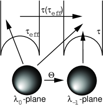
Figure 1: Relation between $\tau_{\hbox{\tiny eff}}$ and $\tau$. $z=\lambda_{-1}=-1+2/\lambda_{0}$

In order to integrate (3) one notices [11] that any solution of (8) can be written as a quotient

$$\tau(z)=\frac{(u_{1}(z)+du_{2}(z))}{(eu_{1}(z)+fu_{2}(z))},$$ (20)

where $u_{1},u_{2}$ are two linearly independent solutions of the hypergeometric differential equation

$$(1+z)(1-z)\frac{d^{2}}{dz^{2}}u(z)+\left((c-2)z+c-2a-2b\right)\frac{d}{dz}u(z)+\frac{2ab}{1+z}=0,$$ (21)

with

$$c=1,\quad\hbox{{;}}\quad b(c-a)+a(c-b)={1\over 2}\quad\hbox{{and}}\quad(a-b)^{2}=\tilde{\alpha}_{1}^{2}.$$ (22)

The coefficients $d,e,f$ in(20) are determined by the asymptotic expansion

$$\tau(z)=\frac{i}{\pi}\ln\frac{z}{2}+\frac{i}{8\pi}z^{-2}\left(-\frac{5}{2}+\frac{7}{3^{6}}\right)+O(z^{-4}).$$ (23)

Finally we substitute $z$ in (20) by

$$z(\tau_{\hbox{\tiny eff}})\equiv\lambda_{-1}=\frac{2}{\lambda_{0}(\tau_{\hbox{\tiny eff}})}-1,$$ (24)

where $\lambda_{0}$ is the automorphic function

$$\tau_{\hbox{\tiny eff}}^{-1} : \tau_{\hbox{\tiny eff}}\mapsto\lambda_{0}\in{\bf C},$$ (25)

$$\lambda_{0}(\tau_{\hbox{\tiny eff}}) = 16q_{e}\prod_{n=1}^{\infty}\left(\frac{1+q_{e}^{2n}}{1+q_{e}^{2n-1}}\right)^{8}\quad\hbox{{ with }}\quad q_{e}=\exp(i\pi\tau_{\hbox{\tiny eff}}).$$

This then integrates (3). To extract the instanton coefficients one needs the inverse map $\tau_{\hbox{\tiny eff}}(\tau)$. This can be done iteratively. We have done this to $O(q^{4})$ allowing us to predict the $4$-instanton coefficient

$$c_{4}=\frac{i}{\pi}\frac{7\cdot 17\cdot 421}{2^{6}\cdot 3^{10}\cdot 521}.$$ (26)

We close with the observation that globally the inverse function $\tau_{\hbox{\tiny eff}}(\tau)$ cannot be single valued. Indeed, existence of a single valued inverse function $z(\tau)$ requires $\tilde{\alpha}_{1}\!=\!p$ or $\alpha\!=\!1/p$, $p\in{\bf Z}$ [11]. As a consequence, the instanton corrected effective coupling $\tau_{\hbox{\tiny eff}}(\tau)$ has a cut somewhere in the strong coupling region. It would certainly be interesting to understand the origin of this branch cut from the non-perturbative physics of this model. Thus far this remains elusive to us.

Acknowledgements:

I.S. would like to thank the Department of Mathematics at Kings College London for hospitality during the writing up of this work. I.S. was supported by a Swiss Government TMR Grant, BBW Nr. 970557.

References

- [1] N. Seiberg and E. Witten, Nucl. Phys. B426 (1994) 19, (E) B430 (1994) 485.
- [2] N. Seiberg and E. Witten, Nucl. Phys. B431 (1994) 484.
- [3] A. Klemm, W. Lerche, S. Theisen and S. Yankielowicz, Phys. Lett. B344 (1995) 169, Int. Jour. Mod. Phys. A11 (1996) 1929; P.C. Argyres and A.E. Faraggi, Phys. Rev. Lett. 74 (1995) 3931; P.C. Argyres and M.R. Douglas, Nucl. Phys. B448 (1995) 93; U.H. Danielsson and B. Sundborg, Phys. Lett. B358 (1995) 273.
- [4] see e.g. P.C. Argyres and M.R. Douglas, Nucl. Phys. B448 (1995) 93, A. Gorsky et al., Phys. Lett. B355 (1995) 466
- [5] E. Witten, Nucl. Phys. B500 (1997) 3; A. Brandhuber, J. Sonnenschein, S. Theisen and S. Yankielowicz, Nucl. Phys. B502 (1997) 125.
- [6] R. Flume, M. Magro, L.O’Raifeartaigh, I. Sachs and O. Schnetz, Nucl. Phys. B494 (1997) 331; M. Magro, L.O’Raifeartaigh and I. Sachs, Nucl. Phys. B508 (1997) 433; G. Bonelli, M. Matone and M. Tonin, Phys. Rev. D55 (1997) 6466.
- [7] N. Dorey, V.V. Khoze and M.P. Mattis, Phys. Rev. D54 (1996) 7832.
- [8] J. Erlich, A. Naqvi, L. Randall, Phys. Rev. D58 (1998) 046002.
- [9] Philip C. Argyres, Adv. Theor. Math. Phys. 2 (1998) 293; J. A. Minahan Nucl. Phys. B537 (1999) 243; Philip C. Argyres, Alex Buchel, Phys. Lett. B442 (1998) 180.
- [10] Z. Nehari, Conformal Mapping, 1st Edition, McGraw-Hill, N.Y. (1952).
- [11] A. Erdelyi (ed.); Higher Transcendental Functions; McGraw Hill (1953)