IASSNS-HEP-99/51

CU-TP-953

PUPT-1855

hep-th/9910001

Approximations for strongly-coupled supersymmetric quantum mechanics

Daniel Kabat^1,2  and Gilad Lifschytz³

¹School of Natural Sciences

Institute for Advanced Study, Princeton, NJ 08540

kabat@sns.ias.edu

²Department of Physics

Columbia University, New York, NY 10027

³Department of Physics

Princeton University, Princeton, NJ 08544

gilad@viper.princeton.edu

We advocate a set of approximations for studying the finite temperature behavior of strongly-coupled theories in 0+1 dimensions. The approximation consists of expanding about a Gaussian action, with the width of the Gaussian determined by a set of gap equations. The approximation can be applied to supersymmetric systems, provided that the gap equations are formulated in superspace. It can be applied to large-$N$ theories, by keeping just the planar contribution to the gap equations.

We analyze several models of scalar supersymmetric quantum mechanics, and show that the Gaussian approximation correctly distinguishes between a moduli space, mass gap, and supersymmetry breaking at strong coupling. Then we apply the approximation to a bosonic large-$N$ gauge theory, and argue that a Gross-Witten transition separates the weak-coupling and strong-coupling regimes. A similar transition should occur in a generic large-$N$ gauge theory, in particular in 0-brane quantum mechanics.

1 Introduction

Recent developments have made it clear that at a non-perturbative level string or M-theory often has a dual description in terms of large-N gauge theory [1, 2]. This has many interesting implications, both for string theory and for the behavior of large-N gauge theory. These developments have been reviewed in [3].

A general property of these dualities is that semiclassical gravity can be used only in regimes where the gauge theory is strongly coupled. For certain terms in the effective action, which are protected by supersymmetry [4], a weak coupling calculation in the gauge theory can be extrapolated to strong coupling and compared to supergravity [5, 6, 7, 8]. But in general non-perturbative methods must be used to analyze the gauge theory in the supergravity regime. Although this reflects the power of duality, as providing a solution to strongly coupled gauge theory, it is also a source of frustration. For example, one would like to use the duality to understand black hole dynamics in terms of gauge theory [9, 10, 11, 12, 13, 14, 15, 16, 17, 18, 19, 20, 21, 22]. But progress along these lines has been hampered by our inadequate understanding of gauge theory.

Thus we would like to have direct control over the gauge theory at strong coupling. Such control is presumably easiest to achieve in a low-dimensional setting. The specific system we have in mind is 0-brane quantum mechanics [23], in the temperature regime where it is dual to a 10-dimensional non-extremal black hole [24]. The dual supergravity makes definite predictions for the partition function of this gauge theory. In the temperature regime under consideration, the partition function is in principle given by the sum of planar diagrams. Although directly summing all planar diagrams seems like a hopeless task, one might hope for a reasonable approximation scheme, which can be used to resum a sufficiently large class of diagrams to see agreement with supergravity.

In this paper we develop a set of approximations which, we hope, can eventually be used to do this. Essentially we self-consistently resum an infinite subset of the perturbation series. These methods have a long history in many-body physics [25] and field theory [26, 27], and have been used to study QCD [28, 29], large-N gauge theory [30], and even supersymmetry breaking [31]. The basic idea is to approximate the theory of interest with a Gaussian action. The Gaussian action is (in general) non-local in time, with a variance that is determined by solving a set of gap equations. One can systematically compute corrections to this approximation, in an expansion about the Gaussian action. To study large-N theories in this formalism, one keeps only the planar contribution to the gap equations. To study supersymmetric systems, we will see that one needs to formulate the gap equations in superspace: loop corrections to the auxiliary fields must be taken into account in order for the approximation to respect supersymmetry.

An outline of this paper is as follows. In section 2 we illustrate the approximation in the simple context of $0+0$ dimensional $\phi^{4}$ theory, and discuss various ways of formulating gap equations. We also discuss (but do not resolve) the difficulties with implementing gauge symmetry in the Gaussian approximation. In section 3 we turn to a series of quantum mechanics problems with ${\cal N}=2$ supersymmetry but no gauge symmetry, and show that the Gaussian approximation captures the correct qualitative strong-coupling behavior present in these simple systems. In section 4 we discuss large-$N$ gauge theories in $0+1$ dimensions, and argue that generically a Gross-Witten transition is present, which separates the weak-coupling and strong-coupling phases. In section 5 we apply the Gaussian approximation to two large-$N$ quantum mechanics problems: a bosonic gauge theory, and a supersymmetric matrix model with a moduli space. We discuss the relevance of these results for 0-brane quantum mechanics.

2 Formulating the Gaussian approximation

2.1 A simple example: $\phi^{4}$ theory in $0+0$ dimensions

Our approach to studying strongly-coupled low-dimensional systems can be illustrated in the following simple context. Consider $0+0$ dimensional $\phi^{4}$ theory, with action

$$S={1\over g^{2}}\left({1\over 2}\phi^{2}+{1\over 4}\phi^{4}\right)\,.$$ (1)

The partition function is given in terms of a Bessel function, by

$$Z=e^{-BF}=\int_{-\infty}^{\infty}d\phi\,e^{-S}={1\over\sqrt{2}}e^{1/8g^{2}}K_{1/4}\left({1\over 8g^{2}}\right)\,.$$ (2)

Expanding this result for weak coupling one obtains an asymptotic series for the free energy.

$$\beta F=-{1\over 2}\log\left(2\pi g^{2}\right)+{3\over 4}g^{2}-3g^{4}+{99\over 4}g^{6}+{\cal O}(g^{8})$$ (3)

This series can of course be reproduced by doing conventional perturbation theory in the coupling $g^{2}$.

But suppose we are interested in the behavior of the free energy at strong coupling. From the exact expression we know that this is given by

$$\beta F=-{1\over 2}\log g-\log{\pi\over\Gamma(3/4)}+{\cal O}(1/g)\,.$$ (4)

Is there some approximation scheme that reproduces this result? Clearly working to any finite order in conventional perturbation theory is hopeless. But it turns out that by resumming a subset of the perturbation series one can do much better. To this end consider approximating the theory (1) with the following Gaussian theory.

$$Z_{0} = e^{-\beta F_{0}}=\int_{-\infty}^{\infty}d\phi\,e^{-S_{0}}$$

$$S_{0} = {1\over 2\sigma^{2}}\phi^{2}$$ (5)

The width of the Gaussian $\sigma^{2}$ is for the moment left arbitrary. By writing

$$Z=\int d\phi\,e^{-S_{0}}e^{-(S-S_{0})}$$

one obtains the identity

$$\beta F=\beta F_{0}\,\,-<e^{-(S-S_{0})}-1>_{{\hbox{\cmsss C}},0}$$ (6)

where the subscript ${\hbox{\cmss C}},0$ denotes a connected expectation value in the Gaussian theory (5). By expanding this identity in powers of $S-S_{0}$ we obtain a reorganized perturbation series

$$\beta F=\beta F_{0}+<S-S_{0}>_{0}-{1\over 2}<(S-S_{0})^{2}>_{{\hbox{\cmsss C}},0}+\cdots\,.$$ (7)

The first few terms are given by

$$\beta F_{0}=-{1\over 2}\log 2\pi\sigma^{2}$$

$$<S-S_{0}>={1\over 2}\left({\sigma^{2}\over g^{2}}-1\right)+{3\sigma^{4}\over 4g^{2}}$$

$$-{1\over 2}<\left(S-S_{0}\right)^{2}>_{{\hbox{\cmsss C}},0}=-{1\over 4}\left({\sigma^{2}\over g^{2}}-1\right)^{2}-{3\sigma^{4}\over 2g^{2}}\left({\sigma^{2}\over g^{2}}-1\right)-{3\sigma^{8}\over g^{4}}\,.$$

The identity (6) holds for any choice of $S_{0}$. But we wish to truncate the series (7), and the truncated series depends on the value of $\sigma^{2}$. So we need a prescription for fixing $\sigma^{2}$. One reasonable prescription is as follows. Consider the Schwinger-Dyson equation

$$<\phi{\delta S\over\delta\phi}>=<{1\over g^{2}}\left(\phi^{2}+\phi^{4}\right)>=1\,.$$

This is an exact relation among correlation functions in the full theory. It seems reasonable to ask that the same relation hold in the Gaussian theory, that is, to require that $<{1\over g^{2}}\left(\phi^{2}+\phi^{4}\right)>_{0}=1$. This implies that $\sigma^{2}$ obeys the gap equation

$${1\over\sigma^{2}}={1\over g^{2}}+{3\sigma^{2}\over g^{2}}\,.$$ (8)

This equation has a simple diagrammatic interpretation, shown in Fig. 1: it self-consistently resums certain self-energy corrections to the $\phi$ propagator.

Figure 1: The gap equation for the $\phi$ propagator. Heavy lines are the dressed propagator $\sigma^{2}$ and thin lines are the bare propagator $g^{2}$.

At weak coupling the gap equation implies $\sigma^{2}=g^{2}+{\cal O}(g^{4})$ and thus the leading term in the Gaussian approximation is

$$\beta F_{0} = -{1\over 2}\log 2\pi g^{2}+{\cal O}(g^{2})\,.$$

This matches the weak coupling behavior seen in (3). At weak coupling the higher order terms in the reorganized perturbation series are small, suppressed by increasing powers of the coupling.

Of course it is not surprising that the Gaussian approximation works well at weak coupling, since at weak coupling the action (1) is approximately Gaussian. But what is rather remarkable is that the Gaussian approximation also gives good results at strong coupling, where the $\phi^{4}$ term in $S$ dominates. At strong coupling the gap equation gives $\sigma^{2}={g\over\sqrt{3}}+{\cal O}(1)$ and thus the leading term in the Gaussian approximation is

$$\beta F_{0}=-{1\over 2}\log g-{1\over 2}\log{2\pi\over\sqrt{3}}+{\cal O}(1/g)\,.$$

Thus $\beta F_{0}$ has the same leading strong-coupling behavior as the exact result (4). Moreover, by reorganizing the perturbation series we have tamed the strong-coupling behavior of perturbation theory. That is, all the higher order terms appearing in the expansion (7) are only ${\cal O}(1)$ at strong coupling.

$$<S-S_{0}>=-{1\over 4}+{\cal O}(1/g)$$

$$-{1\over 2}<(S-S_{0})^{2}>_{{\hbox{\cmsss C}},0}=-{1\over 12}+{\cal O}(1/g)$$

$$\qquad\qquad\qquad\vdots$$

Indeed the first few terms of the reorganized perturbation series fall off nicely with the order. This provides an intrinsic reason to expect that truncating the reorganized perturbation series at low orders should provide a good approximation to the exact result.

2.2 Varieties of gap equations

Consider a set of degrees of freedom $\phi_{i}$, governed by an action $S(\phi_{i})$. We wish to approximate this system with a simpler action $S_{0}(\phi_{i})$. For the most part we will take $S_{0}$ to be Gaussian in the fundamental fields.

$$S_{0}=\sum_{i}{1\over 2\sigma_{i}^{2}}\phi_{i}^{2}$$

But in some situations, in particular for gauge theories, we will be led to use a more general action, which is exactly soluble but not strictly Gaussian, of the form

$$S_{0}=\sum_{a}{1\over\lambda_{a}}{\cal O}_{a}\,.$$

Here the $\lambda_{a}$ are adjustable parameters, and the ${\cal O}_{a}$ are composite operators built out of the fundamental fields.

In either case, the adjustable parameters appearing in $S_{0}$ will be chosen to satisfy a set of gap equations. There are several prescriptions for writing down gap equations. All the gap equations given below have one feature in common: they correspond to critical points of an effective action. We now present several prescriptions for writing down gap equations.

• Lowest-order Schwinger-Dyson gap equations

  For a generic degree of freedom $\phi_{i}$ one has the Schwinger-Dyson equation

  $$<\phi_{i}{\delta S\over\delta\phi_{i}}>=1$$ (9)

  (no sum on $i$). This is an exact relation among correlation functions in the full theory, which can be derived by the standard procedure sketched in section 2.1. It seems natural to choose the parameters of $S_{0}$ in such a way that the same relation holds between correlation functions evaluated in $S_{0}$. That is, a natural set of gap equations corresponds to demanding that for each $i$

  $$<\phi_{i}{\delta S\over\delta\phi_{i}}>_{0}=1\,.$$ (10)

  This gap equation can be obtained from an effective action, as follows. Assuming that $S_{0}$ is strictly Gaussian, and writing $S$ as a polynomial in the fundamental fields, one can show that the gap equations (10) are equivalent to requiring

  $${\partial\over\partial\sigma_{i}^{2}}\left(\beta F_{0}+<S-S_{0}>_{0}\right)=0\,.$$ (11)

  That is, these gap equations make the first two terms of the perturbation series for $\beta F$ stationary with respect to variations of the $\sigma_{i}^{2}$.

• Operator gap equations

  It is natural to ask that expectation values of the operators ${\cal O}_{a}$ agree when calculated in $S_{0}$ and in $S$:

  $$<{\cal O}_{a}>=<{\cal O}_{a}>_{0}.$$ (12)

  For example, when discussing gauge theories, we will introduce the Wilson loop operator ${\cal O}={\rm Tr}Pe^{i\oint A}$. Then the condition (12) demands that Wilson loops agree when computed in $S_{0}$ and in $S$. As another example, suppose that $S_{0}$ is Gaussian, with ${\cal O}_{i}=\phi_{i}^{2}$. Then (12) means choosing the Gaussian widths $\sigma_{i}^{2}$ to be the exact 2-point functions of the full theory.

  As it stands (12) is not a useful equation. But it can be rewritten as

  $$<{\cal O}_{a}e^{-(S-S_{0})}>_{{\hbox{\cmsss C}},0}=<{\cal O}_{a}>_{0}$$ (13)

  and expanded in powers of $S-S_{0}$. At leading order this condition is trivially satisfied. But at first order we get the gap equation

  $$<{\cal O}_{a}(S-S_{0})>_{{\hbox{\cmsss C}},0}=0\,.$$ (14)

  To relate this to an effective action, note the identities

  $${\partial\over\partial\lambda_{a}}\beta F_{0}=-{1\over\lambda_{a}^{2}}<{\cal O}_{a}>_{0}$$

  $${\partial\over\partial\lambda_{a}}<S-S_{0}>_{0}={1\over\lambda_{a}^{2}}<{\cal O}_{a}(S-S_{0})>_{{\hbox{\cmsss C}},0}+{1\over\lambda_{a}^{2}}<{\cal O}_{a}>_{0}\,.$$

  Thus the gap equation (14) is equivalent to requiring

  $${\partial\over\partial\lambda_{a}}\left(\beta F_{0}+<S-S_{0}>_{0}\right)=0\,.$$ (15)

  Note that if $S_{0}$ is strictly Gaussian then these operator gap equations reduce to (11).

• Variational gap equations

  In some cases gap equations can be obtained from a variational principle. For purely bosonic theories one has a bound on the free energy, that

  $$\beta F\leq\beta F_{0}+<S-S_{0}>_{0}\,.$$

  Thus one can formulate a variational principle, based on minimizing the right hand side of the inequality with respect to $\lambda_{a}$ [32]. Note that the resulting gap equations are equivalent to (15).

The gap equations that we have discussed so far are all essentially equivalent: they follow from varying $\beta F_{0}+<S-S_{0}>_{0}$. Unfortunately, they will not be sufficient to analyze many of the theories of interest in this paper. For example, suppose that $S_{0}$ is purely Gaussian, and that $S$ only has non-trivial 3-point couplings. Such couplings do not contribute to $\beta F_{0}+<S-S_{0}>_{0}$, so the gap equations discussed above are not sensitive to the interactions. But then, if some field is massless at tree level, $\beta F_{0}$ will suffer from an infrared divergence.

To resolve these difficulties, we turn to the

• One-loop gap equations

  The gap equation of section 2.1 resummed an infinite set of Feynman diagrams, involving one-loop self-energy corrections to the propagator. This can be extended to theories with both 3-point and 4-point interactions, as follows. Write $S=S_{II}+S_{III}+S_{IV}+\cdots$ as a sum of 2-point, 3-point, 4-point, $\ldots$ couplings, and assume that $S_{0}$ is strictly Gaussian. Consider the quantity

  $$I_{\rm eff}=\beta F_{0}+<S_{II}-S_{0}>_{0}+<S_{IV}>_{0}-{1\over 2}<(S_{III})^{2}>_{{\hbox{\cmsss C}},0}\,.$$

  Requiring ${\partial\over\partial\sigma_{i}^{2}}I_{\rm eff}=0$ gives a set of gap equations which resum all one-loop self-energy corrections to the propagators, built from both 3-point and 4-point vertices. These gap equations are illustrated in Fig. 2. They are sufficient to cure the infrared divergences for most theories of interest. The quantity $I_{\rm eff}$ can be identified with the 2PI effective action of Cornwall, Jackiw and Tomboulis [27], as calculated in a two-loop approximation.

Figure 2: One-loop gap equations. Heavy lines are dressed propagators and thin lines are bare propagators.

In general it does not seem possible to give a prescription for choosing the best set of gap equations. Indeed it is not even clear what ‘best’ means – it may depend on what one wishes to calculate. For example, in some cases, the variational principle gives the optimal gap equations to use when estimating the free energy. A different set of gap equations will give a worse estimate of the free energy, but may give a better estimate of other quantities, such as 2-point correlations. The only general advice we can offer is that the gap equations must be chosen to cure all the infrared divergences which are present in the model. If possible, the gap equations should also respect all the symmetries of the model.

2.3 Difficulties with gauge symmetry

There is a serious difficulty which one encounters when applying the Gaussian approximation to a gauge theory. The underlying gauge invariance implies Ward identities, which relate different Green’s functions. But the Gaussian approximation often violates these identities, and this can lead to inconsistencies.

To illustrate the problem, consider an action $S(\phi_{i})$ which only has 3-point and 4-point couplings – for example ordinary Yang-Mills theory. We assume that the one-point functions $<\phi_{i}>$ vanish. Then the exact Schwinger-Dyson equations $<\phi_{i}{\delta S\over\delta\phi_{i}}>=1$ can be rewritten in terms of proper (1PI) vertices as shown in Fig. 3 [28, 29, 33].

Figure 3: Schwinger-Dyson equations for a theory with 3-point and 4-point couplings but no tadpoles. The solid blobs are dressed propagators; the empty circles are 1PI vertices. All external lines are amputated.

The one-loop gap equations which we discussed in the previous subsection are a truncation of this system. They correspond to dropping the two-loop contributions to the Schwinger-Dyson equations and approximating the dressed 1PI 3-point vertex with a bare vertex. This truncation works well for many theories, as we will see. But in an abelian gauge theory, for example, a Ward identity relates the dressed 3-point vertex to a dressed propagator. This makes it inconsistent to work with dressed propagators but bare vertices; the inconsistency shows up in the fact that the one-loop gap equations with bare vertices do not have a solution. Methods for dealing with this difficulty have been proposed [28, 29], but they do not seem to be compatible with manifest supersymmetry. An adequate analysis of the 0-brane quantum mechanics calls for a more satisfactory treatment of this issue [34]. In section 5, when we apply the Gaussian approximation to a bosonic large-$N$ gauge theory, we will dodge the issue of Ward identities, by avoiding the use of the full set of one-loop gap equations.

3 Scalar models with supersymmetry

In this section we apply the Gaussian approximation to study the strong-coupling behavior of some quantum mechanics problems having ${\cal N}=2$ supersymmetry but no gauge symmetry. The goal is twofold: to learn how to apply the Gaussian approximation to a supersymmetric system, and to test the Gaussian approximation against some of the well understood strong-coupling dynamics present in these simple systems. The main lesson is that the Gaussian approximation works well, provided that it is formulated in a way which respects supersymmetry. Effectively this requires formulating the Gaussian approximation in superspace: gap equations must be introduced for the auxiliary fields.

3.1 A model with a moduli space

We begin by considering a model with three scalar superfields and a superpotential $W=\Phi_{1}\Phi_{2}\Phi_{3}$. The Minkowski space action is (see Appendix A for supersymmetry conventions)

$$S_{M}={1\over g^{2}}\int dt\,{1\over 2}\dot{\phi}_{a}\dot{\phi}_{a}+i\bar{\psi}_{a}\dot{\psi}_{a}+{1\over 2}f_{a}f_{a}-{1\over 2}f_{a}\phi_{b}\phi_{c}s_{abc}+\phi_{a}\bar{\psi}_{b}\psi_{c}s_{abc}$$

where $s_{abc}=+1$ if $a,b,c$ are distinct, $0$ otherwise. Non-perturbatively it is known that the model has a moduli space of vacua localized along the $\phi_{1}$, $\phi_{2}$, $\phi_{3}$ coordinate axes. Thus the spectrum of the Hamiltonian is continuous from zero, and the free energy falls off like a power law at low temperatures.

In studying this model, our goal is to show that the Gaussian approximation captures this power-law behavior of the free energy at low temperatures. This is not a trivial result, because going to low temperatures is equivalent to going to strong coupling: the coupling constant $g^{2}$ is dimensionful, $g^{2}\sim({\rm length})^{-3}$, so the dimensionless effective coupling is $g_{\rm eff}^{2}=g^{2}/T^{3}$. We henceforth adopt units in which $g^{2}=1$.

We use an imaginary time formalism, Wick rotating according to

$$S_{E}=-iS_{M}\qquad\tau=it\qquad f_{a\,E}=-if_{a\,M}\,.$$

Note that we have to Wick rotate the auxiliary fields in order to make the quadratic terms in the action well-behaved in Euclidean space. Expanding the fields in Fourier modes

$$\phi_{a}(\tau) = {1\over\sqrt{\beta}}\sum_{l\in{\hbox to0.0pt{\cmss Z\hss}\hskip 1.8pt\hbox{\cmss Z}}}\phi^{a}_{l}\,e^{-i2\pi l\tau/\beta}$$

$$\psi_{a}(\tau) = {1\over\sqrt{\beta}}\sum_{r\in{\hbox to0.0pt{\cmss Z\hss}\hskip 1.8pt\hbox{\cmss Z}}+{1\over 2}}\psi^{a}_{r}\,e^{-i2\pi r\tau/\beta}$$

$$f_{a}(\tau) = {1\over\sqrt{\beta}}\sum_{l\in{\hbox to0.0pt{\cmss Z\hss}\hskip 1.8pt\hbox{\cmss Z}}}f^{a}_{l}\,e^{-i2\pi l\tau/\beta}$$

the Euclidean action is

$$S_{E} = {1\over 2}\sum_{l}\left({2\pi l\over\beta}\right)^{2}\phi_{l}^{a}\phi_{-l}^{a}+\sum_{r}-i{2\pi r\over\beta}\bar{\psi}_{r}^{a}\psi_{r}^{a}+{1\over 2}\sum_{l}f_{l}^{a}f_{-l}^{a}$$

$$\qquad+{i\over 2\sqrt{\beta}}\sum_{l+m+n=0}\phi_{l}^{a}\phi_{m}^{b}f_{n}^{c}s_{abc}-{1\over\sqrt{\beta}}\sum_{l-r+s=0}\phi_{l}^{a}\bar{\psi}_{r}^{b}\psi_{s}^{c}s_{abc}\,.$$

For a Gaussian action we take (the $R$-parity symmetry discussed in Appendix A forbids any $\phi$ – $f$ mixing)

$$S_{0}=\sum_{l}{1\over 2\sigma_{l}^{2}}\phi_{l}^{a}\phi_{-l}^{a}+\sum_{l}{1\over 2\tau_{l}^{2}}f_{l}^{a}f_{-l}^{a}+\sum_{r}{1\over g_{r}}\bar{\psi}_{r}^{a}\psi_{r}^{a}\,.$$

Next we need to choose a set of gap equations. This model only has cubic interactions, so a reasonable choice is the one-loop gap equations discussed in section 2.2. These read

$${1\over\sigma^{2}_{l}} = \left({2\pi l\over\beta}\right)^{2}+{2\over\beta}\sum_{m+n=l}\sigma_{m}^{2}\tau_{n}^{2}-{2\over\beta}\sum_{r-s=l}h_{r}h_{s}$$

$${1\over\tau_{l}^{2}} = 1+{1\over\beta}\sum_{m+n=l}\sigma_{m}^{2}\sigma_{n}^{2}$$ (16)

$${1\over h_{r}} = {2\pi r\over\beta}+{2\over\beta}\sum_{l+s=r}\sigma_{l}^{2}h_{s}$$

where $h_{r}=-ig_{r}$ is real. Note that time-reversal invariance requires the symmetry properties

$$\sigma^{2}_{-l}=\sigma^{2}_{l}\qquad\tau^{2}_{-l}=\tau^{2}_{l}\qquad h_{-r}=-h_{r}\,.$$

Meanwhile the first few terms in the reorganized perturbation series for the free energy are

$$\beta F_{0}=-{3\over 2}\sum_{l}\log\sigma_{l}^{2}-{3\over 2}\sum_{l}\log\tau_{l}^{2}+{3\over 2}\sum_{r}\log h_{r}^{2}$$

$$<S-S_{0}>_{0}={3\over 2}\sum_{l}\left(({2\pi l\over\beta})^{2}\sigma_{l}^{2}-1\right)+{3\over 2}\sum_{l}\left(\tau_{l}^{2}-1\right)-3\sum_{r}\left({2\pi r\over\beta}h_{r}-1\right)$$

$$-{1\over 2}<(S-S_{0})^{2}>_{{\hbox{\cmsss C}},0}=-{3\over 4}\sum_{l}\left(({2\pi l\over\beta})^{2}\sigma_{l}^{2}-1\right)^{2}-{3\over 4}\sum_{l}\left(\tau_{l}^{2}-1\right)^{2}$$

$$\qquad\qquad+{3\over 2}\sum_{r}\left({2\pi r\over\beta}h_{r}-1\right)^{2}+{3\over 2\beta}\sum_{l+m+n=0}\sigma_{l}^{2}\sigma_{m}^{2}\tau_{n}^{2}-{3\over\beta}\sum_{l-r+s=0}\sigma_{l}^{2}h_{r}h_{s}\,.$$

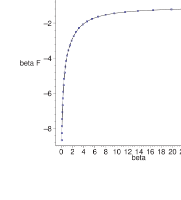
Figure 4: $\beta F$ vs. $\beta$ for the $\Phi_{1}\Phi_{2}\Phi_{3}$ model, as given by the sum of the first three terms of the reorganized perturbation series. Numerical calculations were performed at the indicated points.

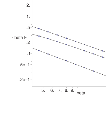
Figure 5: Plots of $(-)$ individual terms in the free energy vs. $\beta$ in the low temperature regime. The scale is $\log$–$\log$, and we shifted $\beta F_{0}$ by a constant to display its power-law behavior. The top curve is $-<S-S_{0}>_{0}$, the middle curve is $+{1\over 2}<(S-S_{0})^{2}>_{{\hbox{\cmsss C}},0}$, and the bottom curve is $-(\beta F_{0}+1.04)$.

To solve the gap equations (16) one has to resort to numerical methods. An effective technique is to start by solving the gap equations analytically at high temperatures, where the loop sums are dominated by the bosonic zero modes $\sigma_{l=0}^{2}$, $\tau^{2}_{l=0}$. One can then repeatedly use the Newton-Raphson method [35] to solve the system at a sequence of successively smaller temperatures, using the solution at inverse temperature $\beta$ as the starting point for Newton-Raphson at $\beta+\Delta\beta$. Further details on the numerical algorithm are given in appendix B.

We have solved this system numerically up to $\beta=28.5$, corresponding to a dimensionless coupling $g_{\rm eff}^{2}=g^{2}\beta^{3}\approx 10^{4}$. The resulting free energy

$$\beta F\approx\beta F_{0}+<S-S_{0}>_{0}-{1\over 2}<(S-S_{0})^{2}>_{{\hbox{\cmsss C}},0}$$ (17)

is shown in Fig. 4. From the plot it seems clear that the energy of the system – given by the slope of $\beta F$ – vanishes as the temperature goes to zero, so the Gaussian approximation has captured the fact that supersymmetry is unbroken in this model. Note that loop corrections to the auxiliary field propagators were crucial in obtaining this result – if we had formulated a Gaussian approximation just for the physical degrees of freedom, the approximation itself would have explicitly broken supersymmetry.

Moreover, in the low-temperature regime, the numerical results for the individual terms in the free energy are well fit by

$$\beta F_{0}=-1.04-0.705\beta^{-1.16}$$

$$<S-S_{0}>_{0}=-2.58\beta^{-1.11}$$ (18)

$$-{1\over 2}<(S-S_{0})^{2}>_{{\hbox{\cmsss C}},0}=-1.77\beta^{-1.11}\,.$$

This behavior can be seen in Fig. 5, where we have plotted these quantities on a $\log$–$\log$ scale.

Evidently $\beta F_{0}$ approaches a non-zero constant at low temperatures, indicating an effective ground-state degeneracy of the system. It would be interesting to understand whether such a degeneracy is really present, or whether it is perhaps an artifact of the Gaussian approximation.

What is more interesting for our purposes is that the subleading behavior of $\beta F_{0}$, as well as the corrections $<S-S_{0}>_{0}$ and $-{1\over 2}<(S-S_{0})^{2}>_{{\hbox{\cmsss C}},0}$, all vanish like a power law at low temperatures, with about the same exponent. It seems plausible that all the higher-order corrections will also follow roughly the same power law. If this is the case then the Gaussian approximation provides a good estimate of the exponent. The coefficient in front of the power law is more difficult to obtain, but one might hope that keeping just the first three terms as in (17) is not such a bad approximation. This leads to a numerical fit

$$\beta F\approx-1.04-4.77\beta^{-1.09}\,.$$

3.2 A model with a mass gap

Next we consider a model containing a single scalar superfield with superpotential $W={1\over 4}\Phi^{4}$, corresponding to the Minkowski action

$$S_{M}={1\over g^{2}}\int dt\,{1\over 2}\dot{\phi}^{2}+i\bar{\psi}\dot{\psi}+{1\over 2}f^{2}-f\phi^{3}+3\phi^{2}\bar{\psi}\psi\,.$$

Non-perturbatively this theory is known to have a unique supersymmetric vacuum localized near $\phi=0$ [36]. In this section we study the finite temperature behavior of this model using the Gaussian approximation, and show that it reproduces this known behavior in the limit of zero temperature. Moreover we will use the Gaussian approximation to obtain an estimate for the energy gap to the first excited state of the system. This is non-trivial because, just as in the previous section, going to low temperature is equivalent to going to strong coupling: the dimensionless effective coupling is $g_{\rm eff}^{2}=g^{2}/T^{2}$. From now on we set $g^{2}=1$.

The Euclidean action in Fourier modes reads

$$S_{E} = \sum_{l}{1\over 2}\left({2\pi l\over\beta}\right)^{2}\phi_{l}\phi_{-l}+\sum_{r}-i{2\pi r\over\beta}\bar{\psi}_{r}\psi_{r}+\sum_{l}{1\over 2}f_{l}f_{-l}$$

$$\quad+{i\over\beta}\sum_{l+m+n+o=0}\phi_{l}\phi_{m}\phi_{n}f_{o}-{3\over\beta}\sum_{l+m-r+s=0}\phi_{l}\phi_{m}\bar{\psi_{r}}\psi_{s}\,.$$

For a Gaussian action we take

$$S_{0}={1\over 2}\sum_{l}\left(\matrix{\phi_{l}&f_{l}\cr}\right)\left(\matrix{\sigma^{2}_{l}&\rho_{l}\cr\rho_{l}&\tau^{2}_{l}\cr}\right)^{-1}\left(\matrix{\phi_{-l}\cr f_{-l}\cr}\right)+\sum_{r}{1\over g_{r}}\bar{\psi}_{r}\psi_{r}\,.$$

Note that one has to allow the fields $\phi$ and $f$ to mix in the Gaussian action, because the superpotential breaks the $R$-parity symmetry discussed in appendix A. Thus we have the correlators

$$<\phi_{l}\phi_{m}>_{0} = \sigma_{l}^{2}\delta_{l+m}\qquad<\phi_{l}f_{m}>_{0}=\rho_{l}\delta_{l+m}$$

$$<f_{l}f_{m}>_{0} = \tau_{l}^{2}\delta_{l+m}\qquad<\bar{\psi_{r}}\psi_{s}>_{0}=-g_{r}\delta_{rs}\,.$$

For this model the one-loop gap equations are identical to the lowest-order Schwinger-Dyson gap equations. In either case one obtains the system

$$\left(\matrix{\sigma^{2}_{l}&\rho_{l}\cr\rho_{l}&\tau^{2}_{l}\cr}\right)^{-1} = \left(\matrix{(2\pi l/\beta)^{2}&0\cr 0&1\cr}\right)+\left(\matrix{{6i\over\beta}\sum_{m}\rho_{m}+{6\over\beta}\sum_{r}g_{r}&{3i\over\beta}\sum_{m}\sigma_{m}^{2}\cr{3i\over\beta}\sum_{m}\sigma_{m}^{2}&0\cr}\right)$$

$${1\over g_{r}} = -i{2\pi r\over\beta}-{3\over\beta}\sum_{m}\sigma_{m}^{2}$$ (19)

The solution to the gap equations has the form

$$\sigma^{2}_{l} = {1\over(2\pi\l/\beta)^{2}+m_{b}^{2}}$$

$$\rho_{l} = -im_{f}\sigma_{l}^{2}$$

$$\tau_{l}^{2} = 1-m_{f}^{2}\sigma_{l}^{2}$$

$$g_{r} = {1\over-i2\pi r/\beta-m_{f}}$$

parameterized by effective bose and fermi masses $m_{b}$, $m_{f}$. It is convenient to introduce the size of the state

$$R_{\rm rms}^{2} = <\phi(\tau)^{2}>$$

$$= {1\over\beta}\sum_{l}\sigma_{l}^{2}$$

$$= {1\over 2m_{b}\tanh(\beta m_{b}/2)}\,.$$

The gap equations then imply consistency conditions which fix $m_{b}$, $m_{f}$ as functions of the temperature.

$$m_{b}^{2} = 27R_{\rm rms}^{4}-3\tanh(3\beta R_{\rm rms}^{2}/2)$$

$$m_{f} = 3R_{\rm rms}^{2}$$ (21)

Meanwhile the first two terms in the expression for the free energy are

$$\beta F_{0}=-{1\over 2}\sum_{l}\log\left(\sigma_{l}^{2}\tau_{l}^{2}-\rho_{l}^{2}\right)+{1\over 2}\sum_{r}\log|g_{r}|^{2}$$

$$<S-S_{0}>_{0}={1\over 2}\sum_{l}\left(({2\pi l\over\beta})^{2}\sigma_{l}^{2}-1\right)+{1\over 2}\sum_{l}(\tau_{l}^{2}-1)+\sum_{r}\left(i{2\pi r\over\beta}g_{r}+1\right)$$

$$\qquad\qquad\qquad+{3i\over\beta}\sum_{l}\sigma_{l}^{2}\sum_{m}\rho_{m}+{3\over\beta}\sum_{l}\sigma_{l}^{2}\sum_{r}g_{r}\,.$$

With the help of the gap equations this reduces to

$$\beta F_{0}\,\,+<S-S_{0}>_{0} = \log(2\sinh(\beta m_{b}/2))-\log(2\cosh(\beta m_{f}/2))$$ (22)

$$-{1\over 2}\beta m_{b}^{2}R_{\rm rms}^{2}+{9\over 2}\beta R_{\rm rms}^{6}\,.$$

The nice thing is that if you expand for low temperatures (equivalently strong coupling – recall that the dimensionless coupling is $g_{\rm eff}^{2}=g^{2}/T^{2}$) then the solution to the consistency conditions (3.2), (21) is

$$\beta m_{b}=\sqrt{3\over 2}\,\beta+\sqrt{6}\,\beta e^{-\beta\sqrt{3/2}}+{\cal O}\left(e^{-\beta\sqrt{6}}\right)\,.$$

The corresponding free energy (22) is

$$\beta F_{0}\,\,+<S-S_{0}>_{0}=-2e^{-\beta\sqrt{3/2}}+{\cal O}\left(e^{-\beta\sqrt{6}}\right)\,.$$ (23)

But this is exactly the low temperature expansion one would expect for the free energy of a system with a unique zero energy ground state (a ‘short multiplet’ of the ${\cal N}=2$ supersymmetry) plus a degenerate pair of first excited states with energy $\sqrt{3/2}$ (a ‘long multiplet’ of ${\cal N}=2$).

We conclude by examining the second-order corrections to the free energy of this model. After imposing the gap equations one finds that

$$-{1\over 2}<(S-S_{0})^{2}>_{{\hbox{\cmsss C}},0}=\frac{1}{9}\beta m_{f}^{3}+\frac{9}{\beta^{2}}\sum_{l+m-r+s=0}\!\!\sigma^{2}_{l}\sigma^{2}_{m}g_{r}g_{s}-\frac{12m_{f}^{3}}{\beta^{2}}\sum_{l+m+n+o=0}\!\!\sigma^{2}_{l}\sigma^{2}_{m}\sigma^{2}_{n}\sigma^{2}_{o}\,.$$

The three-loop sums are best evaluated in position space, using ($0\leq\tau\leq\beta$)

$${1\over\beta}\sum_{l}\frac{1}{(2\pi l/\beta)^{2}+m_{b}^{2}}e^{-i2\pi l\tau/\beta} = {\cosh m_{b}(\tau-\beta/2)\over 2m_{b}\sinh(\beta m_{b}/2)}$$

$${1\over\beta}\sum_{r}\frac{1}{-i2\pi r/\beta-m_{f}}e^{-i2\pi r\tau/\beta} = {e^{m_{f}(\tau-\beta/2)}\over 2\cosh(\beta m_{f}/2)},$$

to obtain

$$-{1\over 2}<(S-S_{0})^{2}>_{{\hbox{\cmsss C}},0}=\frac{1}{9}\beta m_{f}^{3}-\frac{9(\beta m_{b}+\sinh\beta m_{b})}{16m_{b}^{3}(1+\cosh\beta m_{f})\sinh^{2}\frac{\beta m_{b}}{2}}$$

$$\qquad\qquad\qquad-\frac{3\beta m_{f}^{2}}{4m_{b}^{5}\sinh^{4}\frac{\beta m_{b}}{2}}(\frac{3}{8}\beta m_{b}+\frac{1}{2}\sinh\beta m_{b}+\frac{1}{16}\sinh 2\beta m_{b})\,.$$

At low temperatures this reduces to

$$-{1\over 2}<(S-S_{0})^{2}>_{{\hbox{\cmsss C}},0}=-2\sqrt{{2\over 3}}\,\beta e^{-\beta\sqrt{3/2}}\,.$$ (24)

Although exponentially suppressed, this larger than the contribution of the first two terms (23) by a factor of $\beta$. Combining the results (23), (24) we see that the expression for the free energy at low temperatures has the form

$$\beta F=-2e^{-\beta\sqrt{3/2}}\left(1+\beta\sqrt{2/3}+\cdots\right)+{\cal O}\left(e^{-\beta\sqrt{6}}\right)\,.$$

Presumably the second-order term can be interpreted as correcting the energy gap to the first excited state. It would be interesting to find a set of gap equations for which the second order term in the free energy is subdominant at low temperatures.

3.3 A model which breaks supersymmetry

Finally, we consider a model with a single scalar superfield and a superpotential $W={1\over 3}\Phi^{3}$, corresponding to the Minkowski action

$$S_{M}={1\over g^{2}}\int dt\,{1\over 2}\dot{\phi}^{2}+{1\over 2}f^{2}+i\bar{\psi}\dot{\psi}-f\phi^{2}+2\phi\bar{\psi}\psi\,.$$

The dimensionless coupling constant is $g_{\rm eff}^{2}=g^{2}/T^{3}$, and we henceforth set $g^{2}=1$.

This model is known to break supersymmetry [36]. This is an effect which cannot happen at any finite order in perturbation theory, but we will see that it is captured by the Gaussian approximation: the ground state energy comes out positive. This provides an interesting contrast to the usual analysis of supersymmetry breaking via instantons [37], which can be applied to this model once a sufficiently large mass perturbation is introduced. A related analysis of supersymmetry breaking in the $O(N)$ $\sigma$-model was carried out by Zanon [31].

The $O(2)$ R-symmetry prohibits any $\phi$ – $f$ mixing, and implies $<\phi>=0$, but allows a tadpole for $f$. The expectation value of $f$ is the order parameter for supersymmetry breaking. To take it into account we shift $f\rightarrow a+\tilde{f}$, with $<\tilde{f}>=0$. The Euclidean action is

$$S_{E} = \frac{1}{2}\sum_{l}\left(\frac{2\pi l}{\beta}\right)^{2}\phi_{l}\phi_{-l}+\frac{1}{2}\sum_{l}\tilde{f}_{l}\tilde{f}_{-l}-\sum_{r}i\frac{2\pi r}{\beta}\bar{\psi}_{r}\psi_{r}$$ (25)

$$-{1\over 2}\beta a^{2}-ia\sqrt{\beta}\tilde{f}_{0}+a\sum_{l}\phi_{l}\phi_{-l}$$

$$+{i\over\sqrt{\beta}}\sum_{l+m+n=0}\tilde{f}_{l}\phi_{m}\phi_{n}-{2\over\sqrt{\beta}}\sum_{l-r+s=0}\phi_{l}\bar{\psi}_{r}\psi_{s}\,.$$

For a Gaussian action we take

$$S_{0}=\sum_{l}{1\over 2\sigma_{l}^{2}}\phi_{l}\phi_{-l}+\sum_{l}{1\over 2\tau_{l}^{2}}\tilde{f}_{l}\tilde{f}_{-l}+\sum_{r}{1\over g_{r}}\bar{\psi}_{r}\psi_{r}\,.$$ (26)

We will use the one-loop gap equations, which read ($h_{r}=-ig_{r}$)

$$\frac{1}{\sigma_{l}^{2}} = \left(\frac{2\pi l}{\beta}\right)^{2}+2a+\frac{4}{\beta}\sum_{m+n=l}\sigma_{m}^{2}\tau_{n}^{2}-\frac{4}{\beta}\sum_{r-s=l}h_{r}h_{s}$$

$$\frac{1}{\tau_{l}^{2}} = 1+\frac{2}{\beta}\sum_{m+n=l}\sigma^{2}_{m}\sigma^{2}_{n}$$ (27)

$$\frac{1}{h_{r}} = \frac{2\pi r}{\beta}+\frac{4}{\beta}\sum_{l+s=r}\sigma^{2}_{l}h_{s}\,.$$

The value of $a$ is fixed by requiring $<\tilde{f}>=0$. At the one loop level this gives

$$a=\frac{1}{\beta}\sum_{l}\sigma^{2}_{l}\,.$$ (28)

Note that in this approximation the order parameter for supersymmetry breaking is the spread of the ground state wavefunction! We approximate the free energy as $\beta F\approx\beta F_{0}+<S-S_{0}>_{0}$, with

$$\beta F_{0}=-{1\over 2}\sum_{l}\log\sigma_{l}^{2}-{1\over 2}\sum_{l}\log\tau_{l}^{2}+{1\over 2}\sum_{r}\log h_{r}^{2}$$

$$<S-S_{0}>_{0}={1\over 2}\sum_{l}\left(({2\pi l\over\beta})^{2}\sigma_{l}^{2}-1\right)+{1\over 2}\sum_{l}\left(\tau_{l}^{2}-1\right)-\sum_{r}\left({2\pi r\over\beta}h_{r}-1\right)$$

$$\qquad\qquad\qquad-{1\over 2}\beta a^{2}+a\sum_{l}\sigma_{l}^{2}\,.$$

Figure 6: Auxiliary field expectation value vs. $\beta$ in the $\Phi^{3}$ model.

The gap equations for this model must be solved numerically. We show the result for $a=<f>$ in Fig. 6. The key point is that $<f>$ approaches a non-zero constant at low temperatures, $<f>\approx 0.50$, so that supersymmetry is indeed broken. This is reflected in a positive slope of $\beta F$, corresponding to positive vacuum energy. The numerical results can be fit at low temperatures by

$$\beta F_{0}=-0.33+0.21\beta$$

$$<S-S_{0}>_{0}=-0.13+0.057\beta$$

$$\beta F\approx-0.46+0.27\beta\,.$$

Note that, although the vacuum energy is non-zero, it is not given by the classical formula $E={1\over 2}<f>^{2}$ – we are at strong coupling and quantum corrections are important.

To conclude, let us note that it is not really necessary to solve the full set of one-loop gap equations to study this model. Rather, it is a reasonable approximation to truncate the gap equations (27) to

$${1\over\sigma_{l}^{2}} = \left({2\pi l\over\beta}\right)^{2}+2a$$

$${1\over\tau_{l}^{2}} = 1$$

$${1\over h_{r}} = {2\pi r\over\beta}$$

while keeping equation (28) for $a$. In this approximation the gap equations are solved by

$$a^{3}={1\over 8\tanh^{2}(\beta\sqrt{a/2})}$$

while the free energy is given by

$$\beta F\approx\beta F_{0}+<S-S_{0}>_{0}=\log\sinh(\beta\sqrt{a/2})-{1\over 2}\beta a^{2}\,.$$

Note that at low temperatures $a\rightarrow 1/2$ and $\beta F\rightarrow{3\over 8}\beta$.

4 Gauge dynamics and the Gross-Witten transition

In this section we discuss a generic feature of large-$N$ gauge theory: the existence of a Gross-Witten transition [38]. We will argue that such a transition separates the weak-coupling and strong-coupling regimes of the gauge theory.

Suppose we have a $0+1$ dimensional $U(N)$ gauge theory at finite temperature. Although the gauge field $A_{0}(\tau)$ has no local degrees of freedom, one can construct a non-local observable by diagonalizing the Wilson line.

$$U=Pe^{i\int_{0}^{\beta}d\tau A_{0}}=\left(\begin{array}[]{ccc}e^{i\alpha_{1}}&&0\\ &\ddots&\\ 0&&e^{i\alpha_{N}}\end{array}\right)$$

The eigenvalues $\alpha_{1},\ldots,\alpha_{N}$ characterize the gauge-invariant degrees of freedom contained in $A_{0}$ (up to permutation by the Weyl group).

As discussed in [39], for most theories the eigenvalue distribution will be quite different at high and low temperatures. This can be understood as a competition between entropy and energy. The Haar measure for the eigenvalues, corresponding to Wilson lines which are uniformly distributed over the $U(N)$ group manifold, is given by [40]

$$\prod_{i}d\alpha_{i}\prod_{i<j}\left(1-\cos(\alpha_{i}-\alpha_{j})\right)\,.$$

The measure vanishes whenever two eigenvalues coincide. So in the absence of any other interactions, the eigenvalues tend to repel each other, and spread out over the circle in order to maximize their entropy.

On the other hand, energetic considerations often lead to attractive interactions between eigenvalues. As a simple example, suppose we minimally couple the gauge field to a massive adjoint scalar field. Integrating out the scalar field produces an additional contribution to the measure for the eigenvalues, given by

$$\prod_{i<j}\det{}^{-1}\left[-\left(\partial_{\tau}+{i\over\beta}(\alpha_{i}-\alpha_{j})\right)^{2}+m^{2}\right]$$

$$=\prod_{i<j}{1\over 2\left(\cosh\beta m-\cos(\alpha_{i}-\alpha_{j})\right)}\,.$$ (29)

In the high temperature regime $\beta m\ll 1$ this gives a strong attraction between eigenvalues, and the eigenvalues will tend to cluster to minimize their energy. But at low temperatures the potential (29) flattens out, and entropy wins: the eigenvalues will spread out around the circle.

This phenomenon seems to be quite generic: eigenvalues will tend to cluster at high temperatures, and spread out at low temperatures. This should happen even in supersymmetric theories. Of course in quantum mechanics at finite $N$ one has smooth crossover between these two qualitatively different behaviors. But in the large $N$ limit a sharp Gross-Witten phase transition should occur when the eigenvalues can first explore the entire circle.

We conclude with a few remarks on this phenomenon in the context of D-brane physics; for a review of the phases of D-brane gauge theories see [41].

1. The phenomenon is well-known, at least for D-branes which are wrapped on a spatial circle. It is responsible for the transition between singly-wound and multiply-wound strings discussed in [42, 43], and the related black hole transitions discussed in [44]. We’ve merely pointed out that at finite temperature the same transition takes place in Euclidean time: 0-brane worldlines can become multiply wound around the time direction. Only the multiply-wound phase corresponds to a black hole.

2. In a T-dual picture the eigenvalues of the holonomy become the positions of D-instantons on the dual circle. At high temperatures the dual circle is large, and the D-instantons tend to cluster. But at low temperatures, when the dual circle is small, the D-instantons will delocalize. Note that only in the low-temperature regime could one hope to describe the configuration as a black hole, using a static solution to the supergravity equations.

   Let us make a crude estimate of the transition temperature from the D-instanton point of view. Consider a system of $N$ D-instantons in IIB string theory with string coupling $g_{B}$ and string length $l_{s}$. Reasoning analogous to [45, 46] shows that in uncompactified space the D-instantons will cluster and fill out a region of size $L\sim(g_{B}N)^{1/4}l_{s}$. Compactifying the time direction on a circle of size $\beta_{B}$, we expect the D-instantons to delocalize if $\beta_{B}<L$. Mapping to type IIA via

   $$\beta_{A}=\alpha^{\prime}/\beta_{B}\qquad\qquad g^{2}_{A}=g^{2}_{B}\alpha^{\prime}/\beta_{B}^{2}$$

   we conclude that the 0-brane worldlines are multiply-wound when

   $$\beta_{A}>\beta_{\rm crit}=(g_{A}N)^{-1/3}l_{s}\equiv(g^{2}_{YM}N)^{-1/3}\,.$$ (30)

3. The transition at $\beta_{\rm crit}$ can be seen in several ways from the supergravity point of view. The background geometry of a system of 0-branes in the decoupling limit is well-defined above $\beta_{\rm crit}$. Below $\beta_{\rm crit}$ the curvature at the horizon exceeds the string scale, and the dual gauge theory becomes weakly coupled [24].

   The transition can also be identified with the Horowitz-Polchinski correspondence point [47]. Consider a non-extremal black hole in ten dimensions with 0-brane charge. Following [12, 14], one can map this to a ten-dimensional Schwarzschild black hole by lifting to eleven dimensions, boosting in the covering space, and recompactifying. We discuss this transformation in Appendix C. If the original charged black hole is at the critical temperature, then the equivalent neutral black hole turns out to have a Schwarzschild radius close to the string scale. That is, the temperature $T_{\rm crit}$ maps to the Horowitz-Polchinski correspondence point, at which a black hole is on the verge of becoming an elementary string state.

4. Although our primary interest is in quantum mechanics, it is natural to suppose that similar transitions happen in other dimensions. For example, consider $3+1$ dimensional ${\cal N}=4$ large-$N$ Yang-Mills on ${\mathbb{R}}^{3}\times S^{1}$. For any non-zero temperature it seems natural to expect that a Gross-Witten transition occurs when the ’t Hooft coupling $\lambda=g^{2}_{YM}N$ is of order one.

To conclude, we expect that Gross-Witten transitions are generically present in large-$N$ gauge theories at finite temperature. In theories with a dual string interpretation this suggests that a phase transition occurs, which separates the non-geometric phase from the phase with a well-defined background geometry (see also [48, 49]).

5 Large-$N$ models in the Gaussian approximation

In this section we use the Gaussian approximation to study some large-$N$ matrix quantum mechanics problems. One motivation for the problems we consider is that they arise as subsectors of the 0-brane quantum mechanics. The 0-brane quantum mechanics can be written in terms of ${\cal N}=2$ superfields as [50] (see Appendix A)

$$S={1\over g^{2}_{\rm YM}}\int dtd^{2}\theta\,{\rm Tr}\Bigl{\{}-{1\over 4}\nabla^{\alpha}{\cal F}_{i}\nabla_{\alpha}{\cal F}_{i}-{1\over 2}\nabla^{\alpha}\Phi_{a}\nabla_{\alpha}\Phi_{a}-{i\over 3}f_{abc}\Phi_{a}[\Phi_{b},\Phi_{c}]\Bigr{\}}\,.$$ (31)

Here ${\cal F}_{i}$ is the field strength constructed from a gauge multiplet $\Gamma_{\alpha}$, the $\Phi_{a}$ are a collection of seven adjoint scalar multiplets transforming in the ${\bf 7}$ of $G_{2}$, and $f_{abc}$ is a suitably normalized totally antisymmetric $G_{2}$-invariant tensor.

In the next section we drop all the fermions, and (with nine scalar fields) study the bosonic sector of this action. In the following section we drop the gauge multiplet $\Gamma_{\alpha}$, and study the supersymmetric dynamics of the scalar multiplets $\Phi_{a}$.

5.1 Bosonic large-$N$ gauge theory

In this section we study a purely bosonic quantum mechanics problem: the reduction of $d+1$ dimensional $U(N)$ Yang-Mills theory to $0+1$ dimensions. We will study this theory at leading order for large $N$ using the Gaussian approximation. The goal is to show that the Gaussian approximation respects ’t Hooft large-$N$ counting, and can capture the Gross-Witten phase transition which we expect to be present. We will also learn a few useful lessons about 0-brane quantum mechanics.

The degrees of freedom of this model consist of $d$ adjoint scalar fields $X_{i}$, coupled to a gauge field $A_{0}$. The Euclidean action is

$$S_{E}={1\over{g^{2}_{YM}}}\int d\tau\,{\rm Tr}\left\{{1\over 2}D_{\tau}X^{i}D_{\tau}X^{i}-{1\over 4}[X^{i},X^{j}][X^{i},X^{j}]\right\}$$ (32)

where $D_{\tau}=\partial_{\tau}+i[A_{0},\,\cdot\,]$. We set $\partial_{\tau}A_{0}=0$, so that $A_{0}={\rm const.}\equiv{1\over\sqrt{\beta}}A_{00}$. Corresponding to this gauge choice we must introduce a system of periodic ghost fields $\alpha$, $\bar{\alpha}$. In Fourier modes the complete action is

$$S_{E} = {1\over 2{g^{2}_{YM}}}\sum_{l}\left({2\pi l\over\beta}\right)^{2}{\rm Tr}(X_{l}^{i}X_{-l}^{i})+{1\over{g^{2}_{YM}}}\sum_{l\not=0}\left({2\pi l\over\beta}\right)^{2}{\rm Tr}(\bar{\alpha}_{l}\alpha_{l})$$

$$\!\!\!\!-{1\over{g^{2}_{YM}\sqrt{\beta}}}\sum_{l}{2\pi l\over\beta}{\rm Tr}(X_{l}^{i}[A_{00},X_{-l}^{i}])+{1\over{g^{2}_{YM}\sqrt{\beta}}}\sum_{l\not=0}{2\pi l\over\beta}{\rm Tr}(\bar{\alpha}_{l}[A_{00},\alpha_{l}])$$

$$\!\!\!\!{1\over 2{g^{2}_{YM}}\beta}\sum_{l}{\rm Tr}([A_{00},X_{l}^{i}][A_{00},X_{-l}^{i}])-{1\over 4{g^{2}_{YM}}\beta}\sum_{l+m+n+o=0}\!\!\!\!\!\!{\rm Tr}([X_{l}^{i},X_{m}^{j}][X_{n}^{i},X_{o}^{j}])\,.$$

Next we need to choose an action $S_{0}$ to use as the basis for the approximation. Up to now we have always taken $S_{0}$ to be quadratic in the fundamental fields. But this is not appropriate for gauge theory, because the eigenvalues of $A_{00}$ are angular variables. So it is better to work with the holonomy

$$U=Pe^{i\oint d\tau A_{0}}=e^{i\sqrt{\beta}A_{00}}\,.$$

The ‘Gaussian’ action we propose to use is

$$S_{0}=-{N\over\lambda}{\rm Tr}(U+U^{\dagger})+\sum_{l}{1\over 2\sigma_{l}^{2}}{\rm Tr}(X_{l}^{i}X_{-l}^{i})-\sum_{l\not=0}{1\over s_{l}}{\rm Tr}(\bar{\alpha}_{l}\alpha_{l})\,.$$

Strictly speaking, we propose to use this action to describe the relative eigenvalues of the $U(N)$ gauge theory. That is, $U$ really takes values in the group $SU(N)/{\mathbb{Z}}_{N}$. But we will largely ignore this distinction, since it does not affect leading large-$N$ counting.

Although the action $S_{0}$ is not strictly Gaussian, it is soluble, at least in the large-$N$ limit: the action for $U$ is the one-plaquette model studied by Gross and Witten [38]. We briefly recall some results. The one-plaquette partition function is

$$Z_{\kern 1.0pt\vbox{\hrule height=0.8pt\hbox{\vrule width=0.8pt\hskip 2.0pt\vbox{\vskip 4.0pt}\hskip 2.0pt\vrule width=0.4pt}\hrule height=0.4pt}\kern 1.0pt} = e^{-\beta F_{\kern 1.0pt\vbox{\hrule height=0.8pt\hbox{\vrule width=0.8pt\hskip 2.0pt\vbox{\vskip 4.0pt}\hskip 2.0pt\vrule width=0.4pt}\hrule height=0.4pt}\kern 1.0pt}}=\int dU\,e^{{N\over\lambda}{\rm Tr}(U+U^{\dagger})}$$

$$\beta F_{\kern 1.0pt\vbox{\hrule height=0.8pt\hbox{\vrule width=0.8pt\hskip 2.0pt\vbox{\vskip 4.0pt}\hskip 2.0pt\vrule width=0.4pt}\hrule height=0.4pt}\kern 1.0pt} = \left\{\begin{array}[]{ll}N^{2}\left(-{2\over\lambda}-{1\over 2}\log{\lambda\over 2}+{3\over 4}\right)&\quad\lambda\leq 2\\ \vskip 5.69054pt\cr-N^{2}/\lambda^{2}&\quad\lambda\geq 2\end{array}\right.$$

with a third-order phase transition at $\lambda=2$. Diagonalizing the holonomy, $U={\rm diag.}(e^{i\alpha_{1}},\ldots,e^{i\alpha_{N}})$, one has the distribution of eigenvalues

$$\rho_{\kern 1.0pt\vbox{\hrule height=0.8pt\hbox{\vrule width=0.8pt\hskip 2.0pt\vbox{\vskip 4.0pt}\hskip 2.0pt\vrule width=0.4pt}\hrule height=0.4pt}\kern 1.0pt}(\alpha)=\left\{\begin{array}[]{ll}{2\over\pi\lambda}\cos{\alpha\over 2}\sqrt{{\lambda\over 2}-\sin^{2}{\alpha\over 2}}&\quad\lambda\leq 2\\ \vskip 5.69054pt\cr{1\over 2\pi}\left(1+{2\over\lambda}\cos\alpha\right)&\quad\lambda\geq 2\end{array}\right.$$

The expectation value of the Wilson loop is

$$<{\rm Tr}U>_{\kern 1.0pt\vbox{\hrule height=0.8pt\hbox{\vrule width=0.8pt\hskip 2.0pt\vbox{\vskip 4.0pt}\hskip 2.0pt\vrule width=0.4pt}\hrule height=0.4pt}\kern 1.0pt}=\left\{\begin{array}[]{ll}N(1-\lambda/4)&\quad\lambda\leq 2\\ \vskip 5.69054pt\cr N/\lambda&\quad\lambda\geq 2\end{array}\right.$$

Finally, the 2-point correlators in $S_{0}$ are given by

$$<A_{00\,AB}A_{00\,CD}>_{0} = \rho_{0}^{2}\delta_{AD}\delta_{BC}$$

$$<X^{i}_{l\,AB}X^{j}_{m\,CD}>_{0} = \sigma_{l}^{2}\delta^{ij}\delta_{l+m}\delta_{AD}\delta_{BC}$$

$$<\bar{\alpha}_{l\,AB}\alpha_{m\,CD}>_{0} = s_{l}\delta_{lm}\delta_{AD}\delta_{BC}$$

where

$$\rho_{0}^{2}={1\over\beta N}\int d\alpha\,\alpha^{2}\rho_{\kern 1.0pt\vbox{\hrule height=0.8pt\hbox{\vrule width=0.8pt\hskip 2.0pt\vbox{\vskip 4.0pt}\hskip 2.0pt\vrule width=0.4pt}\hrule height=0.4pt}\kern 1.0pt}(\alpha)=\left\{\begin{array}[]{ll}{2\over\beta N}\left[{\rm li}_{2}\left(1-{\lambda\over 2}\right)+\left(1-{2\over\lambda}\right)\log\left(1-{\lambda\over 2}\right)-1\right]&\lambda\leq 2\\ \vskip 5.69054pt\cr{1\over\beta N}\left({\pi^{2}\over 3}-{4\over\lambda}\right)&\lambda\geq 2\end{array}\right.$$

involves a dilogarithm.

The first two terms in the expansion of the free energy are given by

$$\beta F_{0}=\beta F_{\kern 1.0pt\vbox{\hrule height=0.8pt\hbox{\vrule width=0.8pt\hskip 2.0pt\vbox{\vskip 4.0pt}\hskip 2.0pt\vrule width=0.4pt}\hrule height=0.4pt}\kern 1.0pt}(\lambda)-{N^{2}d\over 2}\sum_{l}\log\sigma_{l}^{2}+N^{2}\sum_{l\not=0}\log s_{l}$$ (34)

$$<S-S_{0}>_{0}={N\over\lambda}<{\rm Tr}(U+U^{\dagger})>_{\kern 1.0pt\vbox{\hrule height=0.8pt\hbox{\vrule width=0.8pt\hskip 2.0pt\vbox{\vskip 4.0pt}\hskip 2.0pt\vrule width=0.4pt}\hrule height=0.4pt}\kern 1.0pt}+{N^{2}d\over 2}\sum_{l}\left({1\over{g^{2}_{YM}}}({2\pi l\over\beta})^{2}\sigma_{l}^{2}-1\right)$$

$$\qquad+N^{2}\sum_{l\not=0}\left({1\over{g^{2}_{YM}}}({2\pi l\over\beta})^{2}s_{l}+1\right)+{N^{3}d\over{g^{2}_{YM}}\beta}\,\rho_{0}^{2}\sum_{l}\sigma_{l}^{2}+{N^{3}d(d-1)\over 2{g^{2}_{YM}}\beta}\left(\sum_{l}\sigma_{l}^{2}\right)^{2}\,.$$

In writing these expressions we have kept only the leading large-$N$ behavior, coming from planar diagrams.

The next step is to choose a set of gap equations. For this system we adopt the operator gap equations discussed in section 2.2. That is, we will require that $\beta F_{0}+<S-S_{0}>_{0}$ be stationary with respect to variations of the parameters $\lambda$, $\sigma_{l}^{2}$, $s_{l}$.

Let us first consider the gap equation from varying $\sigma_{l}^{2}$, which reads

$${1\over\sigma_{l}^{2}}={1\over{g^{2}_{YM}}}\left({2\pi l\over\beta}\right)^{2}+{2N\over{g^{2}_{YM}}\beta}\rho_{0}^{2}+{2N(d-1)\over{g^{2}_{YM}}\beta}\sum_{l}\sigma_{l}^{2}\,.$$

The solution is $\sigma_{l}^{2}={g^{2}_{YM}}/((2\pi l/\beta)^{2}+m^{2})$, parameterized by an effective thermal mass

$$m^{2}={2N\over\beta}\rho_{0}^{2}+2(d-1)R_{\rm rms}^{2}\,.$$ (35)

Here we have introduced the ‘size’ of the system, defined by the range of eigenvalues of the matrices $X_{i}$.

$$R_{\rm rms}^{2} = {1\over N}{\rm Tr}<(X^{i}(\tau))^{2}>\qquad\hbox{\rm(no sum on $i$)}$$ (36)

$$= {N\over\beta}\sum_{l}\sigma_{l}^{2}$$

$$= {{g^{2}_{YM}}N\over 2m\tanh(\beta m/2)}\,.$$

Next we consider the gap equation for the ghost propagator, which reads

$${1\over s_{l}}=-{1\over{g^{2}_{YM}}}\left({2\pi l\over\beta}\right)^{2}\qquad l\not=0\,.$$

Thus in this approximation the ghosts are free and decoupled. At leading order they make a trivial contribution to the partition function, since in $0+1$ dimensions one has $\det^{\prime}\partial_{\tau}=1$.

Finally, we have the gap equation from varying $\lambda$, which reads

$$\left\{\begin{array}[]{ll}1-\left(1-{2\over\lambda}\right)\log\left(1-\lambda\over 2\right)={g^{2}_{YM}}N\beta/4dR_{\rm rms}^{2}&\quad\lambda\leq 2\\ \vskip 5.69054pt\cr\lambda={g^{2}_{YM}}N\beta/2dR_{\rm rms}^{2}&\quad\lambda\geq 2\,.\end{array}\right.$$ (37)

By making use of the gap equations, the expressions (34) for the free energy can be simplified to

$$\beta F_{0}=\beta F_{\kern 1.0pt\vbox{\hrule height=0.8pt\hbox{\vrule width=0.8pt\hskip 2.0pt\vbox{\vskip 4.0pt}\hskip 2.0pt\vrule width=0.4pt}\hrule height=0.4pt}\kern 1.0pt}(\lambda)+N^{2}d\log(2\sinh(\beta m/2))$$

$$<S-S_{0}>_{0}={2N\over\lambda}<{\rm Tr}U>_{\kern 1.0pt\vbox{\hrule height=0.8pt\hbox{\vrule width=0.8pt\hskip 2.0pt\vbox{\vskip 4.0pt}\hskip 2.0pt\vrule width=0.4pt}\hrule height=0.4pt}\kern 1.0pt}-{\beta Nd(d-1)\over 2{g^{2}_{YM}}}(R_{\rm rms}^{2})^{2}\,.$$ (38)

Before studying these equations further, let us note that this approximation respects ’t Hooft large-$N$ counting. All the factors of ${g^{2}_{YM}}$ and $N$ which appear in these equations are dictated by ’t Hooft counting plus dimensional analysis, and they can be eliminated by introducing the following rescaled dimensionless quantities:

$$\tilde{\beta}=\beta({g^{2}_{YM}}N)^{1/3}$$

$$\tilde{\lambda}=\lambda$$

$$\tilde{\rho}_{0}^{2}=N\rho_{0}^{2}/({g^{2}_{YM}}N)^{1/3}\qquad\tilde{\sigma}_{l}^{2}=N\sigma_{l}^{2}/({g^{2}_{YM}}N)^{1/3}\qquad\tilde{s}_{l}=Ns_{l}/({g^{2}_{YM}}N)^{1/3}$$

$$\widetilde{R}_{\rm rms}^{2}\equiv{1\over\tilde{\beta}}\sum_{l}\tilde{\sigma}_{l}^{2}=R_{\rm rms}^{2}/({g^{2}_{YM}}N)^{2/3}$$

$$\widetilde{\beta F}=\beta F/N^{2}\,.$$ (39)

The ’t Hooft coupling ${g^{2}_{YM}}N$ acts as a unit of $({\rm energy})^{3}$. The effective dimensionless coupling is then ${g^{2}_{YM}}N/T^{3}$, so the system is strongly coupled at low temperatures.

The system of equations (35), (36), (37) suffices to determine $\lambda$ as a function of the temperature. The results for the case of $d=9$ scalar fields are plotted in Fig. 7. Note that a Gross-Witten transition occurs at $\beta=9.0$, the temperature at which $\lambda$ passes through $2$. The approximation suggests that the transition is weakly second-order: the second derivative of $\beta F_{0}+<S-S_{0}>_{0}$ jumps by -0.0053 across the transition. But this may be an artifact of the approximation; a third order phase transition would seem more plausible.

Figure 7: $\lambda$ vs. $\beta$ for bosonic gauge theory with $9$ scalar fields. The temperature is measured in units of the ’t Hooft coupling.

At high temperatures ($T>({g^{2}_{YM}}N)^{1/3}$, or in dimensionless terms $\tilde{T}>1$) the Gaussian approximation gives the behavior (with $\beta F\approx\beta F_{0}+<S-S_{0}>_{0}$)

$$\lambda \approx \left({d-1\over d(2d-1)}\right)^{1/2}\tilde{\beta}^{3/2}$$

$$R_{\rm rms}^{2} \approx ({g^{2}_{YM}}N)^{2/3}\left({2d-1\over 4d(d-1)}\right)^{1/2}\tilde{\beta}^{-1/2}$$

$$\beta F \approx {3\over 4}N^{2}(d-1)\log\tilde{\beta}$$ (40)

$$E \approx {3\over 4}N^{2}(d-1)T$$

This is the expected result in the high temperature regime: the $N^{2}(d-1)$ physical degrees of freedom making up the matrices $X^{i}$ are excited, with an energy per degree of freedom of order the temperature.

At low temperatures ($T<({g^{2}_{YM}}N)^{1/3}$, or in dimensionless terms $\tilde{T}<1$) the Gaussian approximation gives

$$\lambda \approx {(d-1)^{1/3}\over d}\tilde{\beta}$$

$$R_{\rm rms}^{2} \approx {({g^{2}_{YM}}N)^{2/3}\over 2(d-1)^{1/3}}$$

$$\beta F \approx {3\over 8}N^{2}d(d-1)^{1/3}\tilde{\beta}$$ (41)

$$E \approx {3\over 8}N^{2}d(d-1)^{1/3}({g^{2}_{YM}}N)^{1/3}$$

The physics here is equally simple: the $N^{2}d$ oscillators have all been frozen into their ground state. We see that the ground state energy of an individual oscillator is very large, of order $({g^{2}_{YM}}N)^{1/3}$, while the ground state wavefunction of an individual oscillator is extremely narrow, being a Gaussian of width

$$<(\Delta X^{i}_{AB})^{2}>\,\sim\,({g^{2}_{YM}}N)^{1/3}/N\,.$$

It is only when all of the fluctuations are added together in $R_{\rm rms}$ that the system as a whole has a very large ground state size, $R_{\rm rms}\sim({g^{2}_{YM}}N)^{1/3}$.

Before arguing that the Gaussian approximation really does give reliable results for this system, let us pause to compare the behavior of this bosonic system to the behavior expected of 0-brane quantum mechanics [45, 46]. The full 0-brane system corresponds to $d=9$ and differs by including sixteen adjoint fermions. In the high temperature regime, we expect that the fermions can be neglected on general grounds (from the path integral point of view they are squeezed out by their antiperiodic boundary conditions). So the results (40) should be a good approximation to the behavior of 0-branes at high temperature. On the other hand, in the low temperature regime the 0-brane system has a dual supergravity description [24]. The size of the region in which supergravity is valid $\sim({g^{2}_{YM}}N)^{1/3}$ is expected to match the size of the ground state wavefunction of the supersymmetric gauge theory. We see that the scale $({g^{2}_{YM}}N)^{1/3}$ already appears as the size of the bosonic ground state wavefunction. So it seems that including the fermions should not significantly change the size of the wavefunction. The fermions do enter in a crucial way in the supersymmetric theory, however, because they are necessary for cancelling the enormous bosonic ground state energy which appears in (41).

We will now argue that the Gaussian approximation provides a good description of this bosonic gauge theory for all values of the temperature. Of course the Gaussian approximation is good in the high-temperature regime, where the gauge theory is weakly coupled and the action (32) is approximately Gaussian. But it is also a good approximation at low temperatures. To establish this, let us examine the second-order corrections to the ground state energy of the system.

The second-order correction $-{1\over 2}<(S-S_{0})^{2}>_{{\hbox{\cmsss C}},0}$ is a sum of several terms. But contributions involving the gauge field propagator can be neglected at low temperatures, because $\rho_{0}^{2}\rightarrow 0$ as $\beta\rightarrow\infty$ (the zero mode of the gauge field becomes frozen as the circle decompactifies). Most of the remaining terms cancel when the gap equations are imposed, leaving just

$$-{1\over 2}<(S-S_{0})^{2}>_{{\hbox{\cmsss C}},0}$$

$$=-{N^{4}d(d-1)\over g_{YM}^{4}\beta^{2}}\sum_{l+m+n+o=0}\sigma_{l}^{2}\sigma_{m}^{2}\sigma_{n}^{2}\sigma_{o}^{2}$$

$$=-{g_{YM}^{4}N^{4}d(d-1)\beta\over 16m^{5}\sinh^{4}(\beta m/2)}\left({3\over 8}\beta m+{1\over 2}\sinh(\beta m)+{1\over 16}\sinh(2\beta m)\right)$$

(the three-loop integral is easiest to do in position space). Combining this with previous results gives the first three terms in the reorganized perturbation series for the free energy, which in the low temperatures regime reads

$$\beta F={1\over 2}N^{2}d(d-1)^{1/3}\tilde{\beta}\left[1-{1\over 4}-{1\over 16(d-1)}+\cdots\right]\,.$$

As claimed, the higher order terms in reorganized perturbation theory make a small correction to the free energy, even in the strong-coupling, low temperature regime. Based on the size of the second order correction, we can claim to have computed the ground state energy of this system to within roughly one percent accuracy for the case of $9$ scalar fields.

5.2 A supersymmetric large-$N$ scalar model

Consider a set of $N\times N$ Hermitian scalar multiplets $\Phi_{a}$, governed by an action which is a truncation of the 0-brane quantum mechanics (31).

$$S=\frac{1}{{g^{2}_{YM}}}\int dtd^{2}\theta\,{\rm Tr}\left\{-\frac{1}{2}D^{\alpha}\Phi_{a}D_{\alpha}\Phi_{a}-\frac{i}{3}f_{abc}\Phi_{a}[\Phi_{b},\Phi_{c}]\right\}$$ (42)

Here $a=1,\ldots,7$ is an index in the ${\bf 7}$ of $G_{2}$ and $f_{abc}$ is a $G_{2}$-invariant tensor. We will subsequently set ${g^{2}_{YM}}=1$. For a Gaussian action we take

$$S_{0}=\sum_{l}\frac{1}{2\Delta_{l}^{2}}{\rm Tr}\,\phi^{a}_{l}\phi^{a}_{-l}+\sum_{l}\frac{1}{2\epsilon_{l}^{2}}{\rm Tr}\,f^{a}_{l}f^{a}_{-l}+\sum_{r}\frac{1}{g_{r}}{\rm Tr}\,\bar{\psi}^{a}_{r}\psi^{a}_{r}\,.$$ (43)

The one-loop gap equations are evaluated in the large $N$ limit, by keeping only the planar contributions. We find that the gap equations have a familiar form

$$\frac{1}{\Delta^{2}_{l}} = (\frac{2\pi l}{\beta})^{2}+\frac{2A}{\beta}\sum_{m+n=l}\Delta^{2}_{m}\epsilon^{2}_{n}-\frac{2A}{\beta}\sum_{r-s=l}h_{r}h_{s}$$

$$\frac{1}{\epsilon^{2}_{l}} = 1+\frac{A}{\beta}\sum_{m+n=l}\Delta^{2}_{m}\Delta^{2}_{n}$$

$$\frac{1}{h_{r}} = \frac{2\pi r}{\beta}+\frac{2A}{\beta}\sum_{l+s=r}\Delta^{2}_{l}h_{s}$$ (44)

where $h_{r}=-ig_{r}$ is real and $A=14N$.

In fact, in the Gaussian approximation, this $G_{2}$-invariant model is isomorphic to the $\Phi_{1}\Phi_{2}\Phi_{3}$ model studied in section 3.1. The gap equations (44) can be exactly mapped to those of the $\Phi_{1}\Phi_{2}\Phi_{3}$ model by defining

$$\beta_{\rm new} = A^{1/3}\beta$$

$$\Delta^{2}_{\rm new} = A^{2/3}\Delta^{2}$$

$$\epsilon^{2}_{\rm new} = \epsilon^{2}$$

$$h_{\rm new} = A^{1/3}h\,.$$

Restoring units, note that $A$ is essentially the ’t Hooft coupling, so that $\beta_{\rm new}$ is the physical temperature measured in units of the ’t Hooft coupling. With this redefinition one finds that $\beta F_{0}$, $<S-S_{0}>_{0}$ and $<(S-S_{0})^{2}>_{{\hbox{\cmsss C}},0}$ for the $G_{2}$ model transform into the corresponding quantities for the $\Phi_{1}\Phi_{2}\Phi_{3}$ model, up to an overall factor of $7N^{2}/3$. Thus all the results of section 3.1 can be taken over and applied to the $G_{2}$ model. In particular, the free energy falls off as $\beta_{\rm new}^{-1.1}$ at low temperatures.

6 Conclusions

In this paper we’ve discussed an approximation scheme which can be used to study strongly-coupled quantum mechanics problems. We’ve shown that the approximation can be formulated in a way which respects supersymmetry, by introducing gap equations for the auxiliary fields. We’ve also shown that it can be applied to large-$N$ theories: indeed ’t Hooft scaling is automatic, provided that one keeps just the planar contribution to the gap equations.

We used the approximation to study a number of toy models of scalar supersymmetric quantum mechanics, and found that it captures the correct qualitative behavior of the free energy at strong coupling. Moreover, it provides a quantitative estimate of certain quantities, such as the ground state energy or low-lying density of states, which would be difficult to obtain by any other means.

The approximation has difficulty dealing with gauge symmetry, since the gap equations tend to violate the Ward identities. Nonetheless, we were able to study a large-$N$ gauge theory: the bosonic sector of 0-brane quantum mechanics. The Gaussian approximation provides a remarkably accurate description of the ground state of this theory. The approximation also predicts that a Gross-Witten phase transition occurs when the effective coupling is of order one.

We argued that such a phase transition should be present in a generic large-$N$ gauge theory, in particular for the full 0-brane quantum mechanics. This means that the perturbative gauge theory regime of the 0-brane quantum mechanics is separated from the supergravity regime by a mild phase transition. It also suggests that the Horowitz-Polchinski correspondence point is associated with a phase transition.

Of course our motivation for this project was to develop techniques for understanding 0-brane quantum mechanics. We have been able to incorporate many of the necessary ingredients into the approximation, including supersymmetry and large-$N$ counting. But an adequate analysis of the full 0-brane quantum mechanics requires a more satisfactory treatment of gauge invariance [34].

Acknowledgements

We are grateful to Stanley Deser, Misha Fogler, Gerry Guralnik, Roman Jackiw, Anton Kapustin, David Lowe, Samir Mathur, Emil Mottola, Martin Schaden, Vipul Periwal, Marc Spiegelman, Paul Townsend and Daniel Zwanziger for valuable discussions. DK wishes to thank NYU for hospitality while this work was in progress. The work of DK is supported by the DOE under contract DE-FG02-90ER40542 and by the generosity of Martin and Helen Chooljian. GL wishes to thank the Aspen Center for Physics for hospitality while this work was in progress. The work of GL is supported by the NSF under grant PHY-98-02484.

Appendix A Supersymmetry in quantum mechanics

In this appendix we review the superspace construction of ${\cal N}=2$ theories in $0+1$ dimensions.

With ${\cal N}=2$ supersymmetry we have an $SO(2)$ R-symmetry, with spinor indices $\alpha,\beta=1,2$ and vector indices $i,j=1,2$. The $SO(2)_{R}$ Dirac matrices are real, symmetric, and traceless; for example one can choose $\gamma^{1}=\sigma_{1}$ and $\gamma^{2}=\sigma_{3}$ where $\sigma_{1}$ and $\sigma_{3}$ are Pauli matrices. Given two spinors $\psi_{\alpha}$ and $\chi_{\alpha}$, besides the invariant $\psi_{\alpha}\chi_{\alpha}$, one can construct a second invariant which we will denote

$$\psi^{\alpha}\chi_{\alpha}={i\over 2}\epsilon_{\alpha\beta}\psi_{\alpha}\chi_{\beta}\,.$$

${\cal N}=2$ superspace has coordinates $(t,\theta_{\alpha})$ where $\theta_{\alpha}$ is real. Denoting $\theta^{2}=\theta^{\alpha}\theta_{\alpha}$, we normalize $\int d^{2}\theta\,\theta^{2}=1$.

We introduce the supercharges and supercovariant derivatives

$$Q_{\alpha} = {\partial\over\partial\theta_{\alpha}}+i\theta_{\alpha}{\partial\over\partial t}$$

$$D_{\alpha} = {\partial\over\partial\theta_{\alpha}}-i\theta_{\alpha}{\partial\over\partial t}$$

which obey the algebra

$$\{Q_{\alpha},Q_{\beta}\} = 2i\delta_{\alpha\beta}\partial_{t}$$

$$\{Q_{\alpha},D_{\beta}\} = 0$$

$$\{D_{\alpha},D_{\beta}\} = -2i\delta_{\alpha\beta}\partial_{t}\,.$$

The simplest representation of supersymmetry is a real scalar superfield

$$\Phi=\phi+i\psi_{\alpha}\theta_{\alpha}+f\theta^{2}$$

The general action for a collection of scalar superfields $\Phi_{a}$ is

$$S = {1\over g^{2}}\int dtd^{2}\theta\,-{1\over 2}D^{\alpha}\Phi_{a}D_{\alpha}\Phi_{a}-W(\Phi)$$

$$= {1\over g^{2}}\int dt\,\,{1\over 2}\dot{\phi}_{a}^{2}+i\bar{\psi}_{a}\dot{\psi}_{a}+{1\over 2}f_{a}^{2}-{\partial W\over\partial\phi_{a}}f_{a}+{\partial^{2}W\over\partial\phi_{a}\partial\phi_{b}}\bar{\psi}_{a}\psi_{b}$$

where in the second line we have taken complex combinations $\psi_{a}={1\over\sqrt{2}}\left(\psi_{1a}+i\psi_{2a}\right)$, $\bar{\psi}={1\over\sqrt{2}}\left(\psi_{1a}-i\psi_{2a}\right)$.

In some cases we can extend the $SO(2)$ $R$-symmetry to an $O(2)_{R}$, where the extra ${\hbox to0.0pt{\cmss Z\hss}\hskip 1.8pt\hbox{\cmss Z}}_{2}$ (‘$R$-parity’) acts as $\theta_{\alpha}\rightarrow\gamma^{2}_{\alpha\beta}\theta_{\beta}$. Both the measure $d^{2}\theta$ and the kinetic term are odd under $R$-parity. Thus $R$-parity is a symmetry if the superpotential is odd in $\Phi$, with $\Phi\rightarrow-\Phi$ under R-parity.

To describe gauge theories we introduce a real connection on superspace

$$\nabla_{\alpha} = D_{\alpha}+\Gamma_{\alpha}$$

$$\nabla_{t} = \partial_{t}+i\Gamma_{t}$$

with the gauge transformation $\delta_{\Lambda}\Gamma_{\alpha}=i\nabla_{\alpha}\Lambda$, $\delta_{\Lambda}\Gamma_{t}=\nabla_{t}\Lambda$. The corresponding field strengths ${\cal F}_{\alpha\beta}$, ${\cal F}_{\alpha}$ are real superfields given by

$$\{\nabla_{\alpha},\nabla_{\beta}\} = -2i\delta_{\alpha\beta}\nabla_{t}+{\cal F}_{\alpha\beta}$$

$$\{\nabla_{t},\nabla_{\alpha}\} = {\cal F}_{\alpha}$$

We impose the so-called conventional constraint $\delta_{\alpha\beta}{\cal F}_{\alpha\beta}=0$, which implies that ${\cal F}_{\alpha\beta}$ is a vector of $SO(2)_{R}$:

$${\cal F}_{\alpha\beta}=2\gamma^{i}_{\alpha\beta}{\cal F}_{i}\,.$$

This fixes $\Gamma_{t}$ in terms of the spinor connection $\Gamma_{\alpha}$, but does not constrain $\Gamma_{\alpha}$, as the only independent Bianchi identity

$$\nabla_{\alpha}{\cal F}_{i}=-i\gamma^{i}_{\alpha\beta}{\cal F}_{\beta}$$ (45)

is satisfied for any $\Gamma_{\alpha}$.

We write the expansion of $\Gamma_{\alpha}$ in ‘linear’ components as

$$\Gamma_{\alpha}=\chi_{\alpha}+A_{0}\theta_{\alpha}+X^{i}\gamma^{i}_{\alpha\beta}\theta_{\beta}+d\epsilon_{\alpha\beta}\theta_{\beta}+2\epsilon_{\alpha\beta}\lambda_{\beta}\theta^{2}\,.$$

The fields $X^{i}$ are physical scalars, while $\lambda_{\alpha}$ are their superpartners, $d$ is an auxiliary boson, $\chi_{\alpha}$ are auxiliary fermions, and $A_{0}$ is the 0+1 dimensional gauge field. These linear component fields are of primary interest: by using them to formulate the Gaussian approximation we are effectively making a Gaussian approximation in superspace for the superfield $\Gamma_{\alpha}$, and such an approximation is guaranteed to respect supersymmetry. But it is also useful to define the ‘covariant’ component fields

$$X^{i}|_{\rm cov} \equiv {\cal F}^{i}|_{\theta=0}$$

$$= X^{i}+{1\over 2}\gamma^{i}_{\alpha\beta}\chi_{\alpha}\chi_{\beta}\big{|}_{\rm lin}$$

$$\lambda_{\alpha}|_{\rm cov} \equiv {\cal F}_{\alpha}|_{\theta=0}$$

$$= \lambda_{\alpha}+{1\over 2}\dot{\chi}_{\alpha}+{i\over 2}[A_{0},\chi_{\alpha}]-{i\over 2}\gamma^{i}_{\alpha\beta}[X^{i},\chi_{\beta}]+{i\over 2}\epsilon_{\alpha\beta}[d,\chi_{\beta}]-{i\over 2}[\chi_{\alpha},\chi_{\beta}\chi_{\beta}]\big{|}_{\rm lin}$$

$$A_{0}|_{\rm cov} \equiv \Gamma_{t}|_{\theta=0}$$

$$= A_{0}+{1\over 2}\chi_{\alpha}\chi_{\alpha}\big{|}_{\rm lin}\,.$$

These covariant component fields transform in the usual way under conventional gauge transformations, and are neutral under gauge transformations which depend on $\theta$. Written in terms of covariant component fields the SYM action takes a simple form,

$$S_{SYM} = {1\over g^{2}_{\rm YM}}\int dtd^{2}\theta\,{\rm Tr}\left\{-{1\over 4}\nabla^{\alpha}{\cal F}_{i}\nabla_{\alpha}{\cal F}_{i}\right\}$$

$$= {1\over{g^{2}_{YM}}}\int dt\,{\rm Tr}\Bigl{\{}{1\over 2}D_{0}X^{i}D_{0}X^{i}+{1\over 4}[X^{i},X^{j}][X^{i},X^{j}]$$

$$\qquad\qquad\qquad+{i\over 2}\lambda_{\alpha}D_{0}\lambda_{\alpha}-{1\over 2}\lambda_{\alpha}\gamma^{i}_{\alpha\beta}[X^{i},\lambda_{\beta}]\Bigr{\}}\bigg{|}_{\rm cov}$$

where $D_{0}=\partial_{t}+iA_{0}$. In terms of the linear component fields the action would only take this form in Wess-Zumino gauge. We must also introduce a ghost multiplet, for which we adopt the component expansion

$$C=\alpha+\beta_{\alpha}\theta_{\alpha}+\gamma\theta^{2}$$

where $\alpha$ and $\gamma$ are complex Grassmann fields and $\beta_{\alpha}$ is a complex boson. To the SYM action we add the ghost and gauge fixing terms

$$S_{\rm g.f.}+S_{\rm ghost}={1\over g^{2}_{\rm YM}}\int dtd^{2}\theta\,{\rm Tr}\left\{{1\over 2}D^{\alpha}\Gamma_{\alpha}D^{2}D^{\beta}\Gamma_{\beta}+D^{\alpha}\bar{C}\nabla_{\alpha}C\right\}\,.$$

Note that the gauge-fixed action respects $R$-parity.

Appendix B Solving gap equations numerically

The gap equations are an infinite set of coupled non-linear equations which determine the Fourier modes of the propagators. In general we must resort to numerical methods in order to solve them.

An important simplification follows from the fact that quantum mechanics is UV free. Thus at large momenta the propagators have free-field behavior, and at any given value of the temperature we only need to solve the gap equations to determine a finite number of Fourier modes. In the moduli space model of section 3.1 we obtained good results by solving for modes with $-1.8\beta<l,r<1.8\beta$.

We are left with a finite set of equations, which we solved numerically using the Newton-Raphson method. Let us briefly summarize the method. Consider a system of equations

$$F_{i}(x_{1},\ldots,x_{n})=0\qquad i=1,\ldots,n\,.$$ (46)

We start by guessing a solution $\vec{x}_{\rm old}$, and expand $\vec{F}$ to first order around $\vec{x}_{\rm old}$. Solving the linearized equations gives an improved guess

$$\vec{x}_{\rm new}=\vec{x}_{\rm old}+\delta\vec{x}$$ (47)

where

$$\delta\vec{x}=-{\bf J}^{-1}\vec{F}_{\rm old}\qquad\quad{\bf J}_{ij}=\left.\frac{\partial F_{i}}{\partial x_{j}}\right|_{\vec{x}_{\rm old}}$$ (48)

If the initial guess is sufficiently close to a root, this procedure can be iterated a few times and will rapidly converge. We found that five or six iterations gave excellent results in the moduli space model. The Newton-Raphson method does suffer from poor global convergence, but this can be improved using a procedure known as backtracking [35].

Even with backtracking one needs an initial guess that is sufficiently close to the actual solution. One strategy is to start out at high temperatures. Then the gap equations are dominated by the zero modes, and one can obtain an approximate solution analytically. For example, consider the moduli space model. At high temperatures ($\beta\ll 1$) the gap equations are approximately solved by

$$\sigma_{0}^{2} = \sqrt{\beta}\qquad\sigma_{l\not=0}^{2}=(\beta/2\pi l)^{2}$$

$$\tau_{0}^{2} = 1/2\qquad\tau_{l\not=0}^{2}=1$$ (49)

$$h_{r} = \beta/2\pi r$$

This can be used as a starting point for Newton-Raphson. Then one can solve the system at a sequence of successively lower temperatures, using the solution at one temperature as the initial guess for the next temperature. In the moduli space model we found that increasing $\beta$ by a factor of $1.2$ at each step worked well.

The gap equations can also be solved to determine the large-momentum behavior of the propagators at any temperature, up to constants that can be extracted from the numerical solution for the low-momentum modes. For example, in the moduli space model, the propagators at large momenta behave as

$$\sigma_{l}^{2} = {1\over(2\pi l/\beta)^{2}+m^{2}}$$

$$\tau_{l}^{2} = {(2\pi l/\beta)^{2}\over(2\pi l/\beta)^{2}+m^{2}}$$

$$h_{r} = {2\pi r/\beta\over(2\pi r/\beta)^{2}+m^{2}}$$ (50)

where

$$m^{2}=\frac{2}{\beta}\sum_{l=-\infty}^{\infty}\sigma_{l}^{2}\,.$$

Note that the asymptotic forms of the propagators are related in the expected way, given by the naive supersymmetry Ward identities.

In fact the high momentum behavior is important for computing the free energy. Even in quantum mechanics one has to deal with the divergent quantity $\sum_{l}\log\sigma_{l}^{2}$. This sum, which appears in $\beta F_{0}$, can be defined by

$$\sum_{-\infty}^{\infty}\log\big{[}\sigma_{l}^{2}\big{(}(2\pi l/\beta)^{2}+m^{2}\big{)}\big{]}-2\log(2\sinh(\beta m/2))\,.$$ (51)

The modified sum converges, so it can be calculated numerically.

Appendix C Black hole – SYM correspondence

We discuss the connection between ten dimensional Schwarzschild black holes and finite temperature SYM quantum mechanics. We relate the two theories by boosting an eleven dimension black string and recompactifying it on a smaller circle to keep the entropy the same [12, 14]. Although this transformation is not a symmetry of the theory, it does preserve some of its properties, and therefore can be used to identify phenomena on the black hole side with phenomena in the gauge theory.

C.1 Boosted black string

We start with the black string solution in eleven dimensions

$$ds_{11}^{2} = -h(r)dt^{2}+h^{-1}(r)dr^{2}+r^{2}d\Omega_{8}+dz^{2}$$

$$h(r) = 1-\frac{r_{0}^{7}}{r^{7}}\,.$$ (52)

If the eleventh dimension $z$ is compactified on a circle of radius $R$ one can reduce this metric to get the ten dimensional metric of a Schwarzschild black hole in type IIA string theory. The black hole mass and entropy are given by ($l_{p}$ is the eleven dimensional Planck length)

$$M = \frac{\Omega_{8}Rr_{0}^{7}}{l_{p}^{9}}$$

$$S = \frac{\Omega_{8}\pi Rr_{0}^{8}}{2l_{p}^{9}}$$ (53)

where $\Omega_{8}=\frac{2\pi^{9/2}}{\Gamma(9/2)}$.

Following [12, 14] we boost in the $z$ direction (in the covering space) with boost parameter $\alpha$, and recompactify the new $z$ direction on a circle with radius

$$R^{\prime}=\frac{R}{\cosh\alpha}.$$ (54)

This radius is chosen so that the resulting ten dimensional charged black hole will have the same entropy (53) as the Schwarzschild black hole.

In string frame the charged black hole solution is

$$ds^{2} = -f^{-1/2}(r)h(r)dt^{2}+f^{1/2}(r)[h^{-1}(r)dr^{2}+r^{2}d\Omega_{8}^{2}]$$

$$e^{2(\phi-\phi_{\infty})} = f^{3/2}(r)$$

$$A_{0}(r) = \frac{r_{0}^{7}\sinh\alpha\cosh\alpha}{r^{7}+r_{0}^{7}\sinh^{2}\alpha}$$ (55)

$$f(r) = 1+\frac{r_{0}^{7}\sinh^{2}\alpha}{r^{7}}$$

We will eventually take the limit $\alpha\rightarrow\infty$ with $r_{0}$ fixed (this limit was also considered in [51, 52, 53]), so we won’t distinguish between $\sinh\alpha$ and $\cosh\alpha$. In this limit the number of unit charge D0-branes is given by dividing the ADM mass of the black hole by $1/R^{\prime}$,

$$N=\frac{7}{8}MR.$$ (56)

Now let’s consider the string theory parameters that come from this compactification. Our conventions are

$$R=g_{s}l_{s}\qquad\quad l_{s}^{2}=\frac{l_{p}^{3}}{R}\frac{1}{(2^{4}\pi^{7})^{1/3}}\,.$$ (57)

One finds (string parameters are labeled by a tilde)

$$\tilde{l}_{s}^{2} = \frac{l_{p}^{3}\cosh\alpha}{R(2^{4}\pi^{7})^{1/3}}$$

$$\tilde{g}_{s} = \left(\frac{R}{l_{p}\cosh\alpha}\right)^{3/2}(2^{4}\pi^{7})^{1/6}$$ (58)

$$\tilde{g}_{YM}^{2} \equiv \frac{1}{4\pi^{2}}\tilde{g}_{s}\tilde{l}_{s}^{-3}=\frac{(2^{4}\pi^{7})^{1/3}R^{3}}{4\pi^{2}l_{p}^{6}}\cosh^{-3}\alpha.$$

The string length grows with $\alpha$, so we rescale all lengths by $1/\cosh\alpha$. This gives new parameters (labeled by ^′)

$$(l_{s}^{{}^{\prime}})^{2} = \frac{l_{p}^{3}}{R(2^{4}\pi^{7})^{1/3}}\cosh^{-1}\alpha$$

$$g^{{}^{\prime}}_{s} = \tilde{g}_{s}$$

$$(g_{YM}^{{}^{\prime}})^{2} = \frac{R^{3}}{l_{p}^{6}}\frac{(2^{4}\pi^{7})^{2/3}}{4\pi^{2}}$$ (59)

$$r^{\prime} = r/\cosh\alpha.$$

Now taking the limit $\alpha\rightarrow\infty$ brings us into the gauge theory regime with a finite value for the Higgs vev

$$U\equiv\frac{r^{\prime}}{(l_{s}^{{}^{\prime}})^{2}}=r/l_{s}^{2}.$$ (60)

On the supergravity side the change of scale means that

$$ds^{{}^{\prime}2}=\frac{1}{\cosh^{2}\alpha}ds^{2}\,.$$ (61)

Using equations (53,56,59,60) we can write

$$\frac{r_{0}^{7}\sinh^{2}\alpha}{r^{7}}=\frac{d_{0}Ng_{ym}^{{}^{\prime}2}}{U^{7}l_{s}^{{}^{\prime}4}}$$

$$\frac{r_{0}^{7}}{r^{7}}=\frac{9}{16}a_{0}U^{-7}Mg_{ym}^{{}^{\prime}4}=\frac{U_{0}^{7}}{U^{7}}\equiv h(U)-1$$ (62)

where $d_{0}=\Gamma(7/2)2^{7}\pi^{9/2}$ and $a_{0}=\frac{\Gamma(9/2)2^{11}\pi^{13/2}}{9}$.

As $\alpha\rightarrow\infty$ note that $l_{s}^{{}^{\prime}}\rightarrow 0$, so the metric becomes (defining $t=t^{{}^{\prime}}/\cosh\alpha$, $e^{2}=g_{YM}^{{}^{\prime}2}N$)

$$ds^{{}^{\prime}2}=l_{s}^{{}^{\prime}2}[-\frac{U^{7/2}}{d^{1/2}_{0}e}h(U)dt^{2}+h^{-1}(U)\frac{d^{1/2}_{0}e}{U^{7/2}}dU^{2}+d^{1/2}_{0}eU^{-3/2}d\Omega_{8}^{2}]\,.$$ (63)

This is indeed the near horizon geometry of a 0-brane black hole. This analysis is closely related to [54].

C.2 Parameter identification

To give a precise identification between the Schwarzschild black hole and the gauge theory we recall that a near extremal black hole has the following energy density, temperature and entropy density [24].

$$E = a_{p}^{-1}e^{-4}N^{2}U_{0}^{7-9}$$

$$eT = c_{p}U_{0}^{(5-p)/2}$$ (64)

$$S = h_{p}e^{-3}N^{2}U_{0}^{(9-p)/2}$$

Here $e^{2}=g_{YM}^{2}N$, $U_{0}$ is the position of the horizon in Poincaré coordinates, and $p+1$ is the worldvolume dimension of the gauge theory. The constants appearing in these equations are

$$a_{p} = \frac{1}{9-p}\Gamma(\frac{9-p}{2})2^{11-2p}\pi^{\frac{13-3p}{2}}$$

$$h_{p} = (7-p)^{-1/2}\Gamma^{-\frac{1}{2}}(\frac{9-p}{2})2^{p-4}\pi^{\frac{3p-13}{4}}$$ (65)

$$c_{p} = (7-p)^{3/2}\Gamma^{-\frac{1}{2}}(\frac{9-p}{2})2^{p-6}\pi^{\frac{3p-13}{4}}\,.$$

The above equations are only reliable if the supergravity approximation is valid near the horizon of the black hole – that is, if the dilaton is small and the curvature is small in string units. The condition for small curvature near the horizon is $U_{0}^{3-p}\ll e^{2}$, and the point where the curvature is order one is $T\sim U_{0}$. As a passing observation note that while the thermodynamics depends on $p$, one has a relation $E\sim e^{-2}N^{2}T^{2}U_{0}^{2}$ which holds independent of $p$, aside from the exact numerical factor.

Now we can make identifications between the Schwarzschild black hole and the gauge theory. We consider the case $p=0$. On the Schwarzschild black hole side there are three parameters $M$, $R$, $l_{p}$. On the gauge theory side there is $N$, $E$, $g^{2}_{YM}$. By equating the thermodynamics we obtain the relations

$$E=\frac{9}{16}M$$

$$g_{YM}^{2}=\frac{(2^{4}\pi^{7})^{2/3}}{4\pi^{2}}\frac{R^{3}}{l_{p}^{6}}$$

$$N=\frac{7}{8}RM$$

$$T_{\rm gauge}=T_{\rm Schwarzschild}=\frac{7}{4\pi r_{0}}$$ (66)

$$U_{0}=\frac{(2^{4}\pi^{7})^{1/3}Rr_{0}}{l_{p}^{3}}$$

$$S_{\rm gauge}=S_{\rm Schwarzschild}$$

C.3 Transition points

Let’s see what the different regimes of the gauge theory correspond to for the Schwarzschild black hole. It is convenient to use (we drop numerical factors)

$$M = E=N^{2}e^{-6/5}T^{14/5}$$

$$R = N^{-1}e^{6/5}T^{-14/5}$$

$$S = N^{2}e^{-6/5}T^{9/5}$$ (67)

$$l_{p}^{2} = N^{-2/3}e^{8/15}T^{-14/5}$$

There is one issue we would like to comment on. The specific heat of a Schwarzschild black hole is negative, while the gauge theory clearly has a positive specific heat. Nonetheless their thermodynamics can be identified, since we hold different quantities fixed when we take derivatives with respect to the temperature (the temperature is the same on both sides). In the gauge theory we hold $N$ and $g^{2}_{YM}$ fixed, but on the supergravity side we hold $R$ and $l_{p}$ fixed. This is responsible for the difference. Thus the negative specific heat of the Schwarzschild black hole is not in contradiction with its description in terms of thermodynamics of an ordinary field theory (see also [10]).

Now let’s look at some transition points:

1. When $R=r_{0}$ the black string becomes unstable and turns into an eleven dimensional black hole [55]. Our formulas are only appropriate for $R<r_{0}$. At this point one finds

   $$S_{1} = N$$

   $$R_{1} = N^{5/9}e^{-2/3}$$

   $$T_{1} = e^{2/3}N^{-5/9}$$ (68)

   $$l_{p}^{2} = e^{-4/3}N^{2/9}\,.$$

   This is the BFKS point [9, 15].

2. At $R=l_{p}$ the black string is better described as a ten dimensional black hole and the string theory has $g_{s}=1$. At this point

   $$S_{2} = N^{8/7}$$

   $$R_{2} = N^{1/3}e^{-2/3}$$ (69)

   $$T_{2} = e^{2/3}N^{-10/21}\,.$$

3. Consider the point where the Schwarzschild black hole has a horizon size of the order the string length, $r^{2}_{0}=l^{2}_{s}=l_{p}^{3}/R$. We find the corresponding gauge theory parameters

   $$S_{3} = N^{2}$$

   $$R_{3} = e^{-2/3}N^{-1}$$

   $$T_{3} = e^{2/3}$$ (70)

   $$g_{s} = \frac{1}{N}\,.$$

   This is the point where the curvature at the horizon of the charged black hole becomes of order one. Beyond this point the effective coupling of the gauge theory is small. We have argued in this paper that at this point there is a phase transition. We now see that this transition occurs at the Horowitz-Polchinski correspondence point, where the Schwarzschild black hole turns into an elementary string state [47].

References

- [1] T. Banks, W. Fischler, S. Shenker, and L. Susskind, M theory as a matrix model: a conjecture, hep-th/9610043.
-
[2]
J. Maldacena, The large limit of superconformal
field theories and supergravity, hep-th/9711200;
S.S. Gubser, I.R. Klebanov and A.M. Polyakov, Gauge theory correlators from noncritical string theory, hep-th/9802109;
E. Witten, Anti de Sitter space and holography, hep-th/9802150. -
[3]
T. Banks, Matrix theory, Nucl. Phys. Proc. Suppl. 67, 180 (1998),
hep-th/9710231;
W. Taylor, Lectures on D-branes, gauge theory and M(atrices), hep-th/9801182;
O. Aharony, S.S. Gubser, J. Maldacena, H. Ooguri and Y. Oz, Large N field theories, string theory and gravity, hep-th/9905111. -
[4]
S. Paban, S. Sethi and M. Stern, Constraints from extended supersymmetry
in quantum mechanics, Nucl. Phys. B534, 137 (1998), hep-th/9805018;
S. Paban, S. Sethi and M. Stern, Supersymmetry and higher derivative terms in the effective action of Yang-Mills theories, JHEP 06, 012 (1998), hep-th/9806028;
D. Lowe, Constraints on higher derivative operators in the matrix theory effective Lagrangian, hep-th/9810075;
S. Hyun, Y. Kiem and H. Shin, Supersymmetric completion of supersymmetric quantum mechanics, hep-th/9903022;
S. Sethi and M. Stern, Supersymmetry and the Yang-Mills effective action at finite , hep-th/9903049. - [5] K. Becker and M. Becker, A two-loop test of M(atrix) theory, hep-th/9705091.
- [6] K. Becker, M. Becker, J. Polchinski and A. Tseytlin, Higher order graviton scattering in M(atrix) theory, hep-th/9706072.
- [7] Y. Okawa and T. Yoneya, Multibody interactions of D-particles in supergravity and matrix theory, hep-th/9806018.
- [8] W. Taylor and M. van Raamsdonk, Supergravity currents and linearized interactions for matrix theory configurations with fermionic backgrounds, hep-th/9812239.
- [9] T. Banks, W. Fischler, I. R. Klebanov, and L. Susskind, Schwarzschild black holes from matrix theory, hep-th/9709091.
- [10] I. R. Klebanov and L. Susskind, Schwarzschild black holes in various dimensions from matrix theory, hep-th/9709108.
- [11] E. Halyo, Six dimensional Schwarzschild black holes in M(atrix) theory, hep-th/9709225.
- [12] G. Horowitz and E. Martinec, Comments on black holes in matrix theory, hep-th/9710217.
- [13] M. Li, Matrix Schwarzschild black holes in large N limit, hep-th/9710226.
- [14] S. Das, S. Mathur, S. Rama, and P. Ramadevi, Boosts, Schwarzschild black holes and absorption cross-sections in M theory, hep-th/9711003.
- [15] T. Banks, W. Fischler, I. Klebanov, and L. Susskind, Schwarzschild black holes in matrix theory II, hep-th/9711005.
- [16] H. Liu and A.A. Tseytlin, Statistical mechanics of D0-branes and black hole thermodynamics, hep-th/9712063.
- [17] T. Banks, W. Fischler, and I. Klebanov, Evaporation of Schwarzschild black holes in matrix theory, hep-th/9712236.
- [18] N. Ohta and J.-G. Zhou, Euclidean path integral, D0-branes and Schwarzschild black holes in matrix theory, hep-th/9801023.
- [19] M. Li and E. Martinec, Probing matrix black holes, hep-th/9801070.
- [20] D. Lowe, Statistical origin of black hole entropy, hep-th/9802173.
- [21] D. Kabat and G. Lifschytz, Tachyons and black hole horizons in gauge theory, hep-th/9806214.
- [22] D. Kabat and G. Lifschytz, Gauge theory origins of supergravity causal structure, hep-th/9902073.
- [23] M. Claudson and M. Halpern, Supersymmetric ground state wavefunctions, Nucl. Phys. B250 (1985) 689.
- [24] N. Itzhaki, J.M. Maldacena, J. Sonnenschein and S. Yankielowicz, Supergravity and the large limit of theories with sixteen supercharges, hep-th/9802042.
- [25] A. Fetter and J. Walecka, Quantum theory of many-particle systems (McGraw-Hill, 1971).
- [26] L. Dolan and R. Jackiw, Symmetry behavior at finite temperature, Phys. Rev. D9, 3320 (1974).
- [27] J. Cornwall, R. Jackiw and E. Tomboulis, Effective action for composite operators, Phys. Rev. D10, 2428 (1974).
- [28] This approach has been reviewed in C. Roberts and A. Williams, Dyson-Schwinger equations and their applications to hadronic physics, hep-ph/9403224.
- [29] For recent work see L. von Smekal, A. Hauck and R. Alkofer, A solution to coupled Dyson-Schwinger equations for gluons and ghosts in Landau gauge, hep-ph/9707327.
- [30] M. Engelhardt and S. Levit, Variational master field for large- interacting matrix models – free random variables on trial, hep-th/9609216.
- [31] D. Zanon, Spontaneous supersymmetry breaking in leading order, Phys. Lett. B104, 127 (1981).
- [32] R. P. Feynman, Statistical mechanics (Addison-Wesley, 1972), section 3.4.
- [33] J. Bjorken and S. Drell, Relativistic quantum fields (McGraw-Hill, 1965), section 19.3.
- [34] D. Kabat, G. Lifschytz and D. Lowe, in preparation.
- [35] W. Press, S. Teukolsky, W. Vetterling and B. Flannery, Numerical recipes in C, 2nd. ed. (Cambridge, 1992).
- [36] E. Witten, Dynamical breaking of supersymmetry, Nucl. Phys. B185 (1981) 513.
- [37] P. Salomonson and J. van Holten, Fermionic coordinates and supersymmetry in quantum mechanics, Nucl. Phys. B196 (1982) 509.
- [38] D. Gross and E. Witten, Possible third-order phase transition in the large- lattice gauge theory, Phys. Rev. D21, 446 (1980).
- [39] G. Polhemus, Statistical mechanics of multiply wound D-branes, hep-th/9612130.
- [40] M. Mehta, Random matrices, 2nd. ed. (Academic Press, 1991).
- [41] E. Martinec, Black holes and the phases of brane thermodynamics, hep-th/9909049.
- [42] S. Das and S. Mathur, Excitations of D strings, entropy and duality, hep-th/9601152.
- [43] J. Maldacena and L. Susskind, D-branes and fat black holes, hep-th/9604042.
- [44] L. Susskind, Matrix theory black holes and the Gross-Witten transition, hep-th/9805115.
- [45] L. Susskind, Holography in the flat space limit, hep-th/9901079.
- [46] J. Polchinski, M-theory and the light cone, hep-th/9903165.
- [47] G. Horowitz and J. Polchinski, A correspondence principle for black holes and strings, hep-th/9612146.
- [48] V. Periwal, String field theory Hamiltonians from Yang-Mills theories, hep-th/9906052.
- [49] V. Periwal and G. Lifschytz, Dynamical truncation of the string spectrum at finite , hep-th/9909152.
- [50] D. Kabat and S.-J. Rey, Wilson lines and T-duality in heterotic M(atrix) theory, hep-th/9707099.
- [51] S. Hyun, Y. Kiem and H. Shin, Infinite Loretz boost along the M-theory circle and non-asymptotically flat solutions in supergravities, hep-th/9712021.
- [52] F. Englert and E. Rabinovici, Statistical entropy of Schwarzschild black holes, hep-th/9801048.
- [53] R. Argurio, F. Englert and L. Houart, Statistical entropy of the four dimensional Schwarzschild black hole, hep-th/9801053.
- [54] N. Seiberg, Why is the matrix model correct?, hep-th/9710009.
- [55] R. Gregory and R. Laflamme, Black strings and -branes are unstable, Phys. Rev. Lett. 70, 2837 (1993), hep-th/9301052.