MASS SCALES IN STRING AND M-THEORY^†

Abstract

I review the relations between mass scales in various string theories and in M-theory. I discuss physical motivations and possible consistent realizations of large volume compactifications and low string scale.
Large longitudinal dimensions, seen by Standard Model particles, imply in general that string theory is strongly coupled unless its tension is close to the compactification scale. Weakly coupled, low-scale strings can in turn be realized only in the presence of extra large transverse dimensions, seen through gravitational interactions, or in the presence of infinitesimal string coupling. In the former case, quantum gravity scale is also low, while in the latter, gravitational and string interactions remain suppressed by the four-dimensional Planck mass. There is one exception in this general rule, allowing for large longitudinal dimensions without low string scale, when Standard Model is embedded in a six-dimensional fixed-point theory described by a tensionless string.
Extra dimensions of size as large as TeV${}^{-1}\simeq 10^{-16}$ cm are motivated from the problem of supersymmetry breaking in string theory, while TeV scale strings offer a solution to the gauge hierarchy problem, as an alternative to softly broken supersymmetry or technicolor. I discuss these problems in the context of the above mentioned string realizations, as well as the main physical implications both in particle accelerators and in experiments that measure gravity at sub-millimeter distances.

^†Lectures given at the Spring Workshop “on Superstrings and Related Matters”, ICTP, Trieste, Italy, 22-30 March 1999, and at the Advanced School on “Supersymmetry in the Theories of Fields, Strings and Branes”, Sandiago de Compostela, Spain, 26-31 July 1999. A short version was given as an invited talk at Strings 99, Potsdam, Germany, 19-24 July 1999 and at the European Program meeting on “Quantum Aspects of Gauge Theories, Supersymmetry and Unification”, Paris, France, 1-7 September 1999.

September 1999

1 Outline

The outline of this review article is the following:

1.1  Preliminaries
2.   Heterotic string and motivations for large volume compactifications
2.1  Gauge coupling unification
2.2  Supersymmetry breaking by compactification
3.   M-theory on $S^{1}/Z_{2}$“$\times$”Calabi-Yau
4.   Type I/I^′ string theory and D-branes
4.1  Low-scale strings and extra-large transverse dimensions
4.2  Relation type I/I^′ – heterotic
5.   Type II theories
5.1  Low-scale IIA strings and tiny coupling
5.2  Large dimensions in type IIB
5.3  Relation type II – heterotic
6.   Main experimental tests for particle accelerators
6.1  Longitudinal dimensions
6.2  Transverse dimensions and low-scale quantum gravity
6.3  Low-scale strings
7.   Physics
7.1  Gauge hierarchy
7.2  Unification
7.3  Supersymmetry breaking
8.   Gravity modification and sub-millimeter forces
References

1.1 Preliminaries

In critical (ten) dimensions, any consistent superstring theory has two parameters: a mass (or length) scale $M_{s}$ ($l_{s}=M_{s}^{-1}$), and a dimensionless string coupling $\lambda_{s}$ given by the vacuum expectation value (VEV) of the dilaton field $e^{<\phi>}=\lambda_{s}$ [1, 2]:

$$D=10:\qquad\quad M_{s}=l_{s}^{-1}\qquad\lambda_{s}\,.$$ (1)

Upon compactification in $D=4$ dimensions on a compact manifold of volume $V$, these parameters determine the four-dimensional (4d) Planck mass (or length) $M_{p}$ ($l_{p}=M_{p}^{-1}$) and the dimensionless gauge coupling $g$ at the string scale. For simplicity, in the following we drop all numerical factors from our formulae, while, when needed, we use the numerical values:

$$D=4:\qquad\quad M_{p}\simeq 1.2\times 10^{19}\ {\rm GeV}\qquad g\simeq 1/5\,.$$ (2)

Moreover, the weakly coupled condition implies that $\lambda_{s}<<1$. Our method in the following consists in expressing the 10d parameters $(M_{s},\lambda_{s})$ in terms of the 4d ones and the compactification volume, in heterotic ($s=H$), type I ($s=I$) and type II ($s=II$) string theories, and then discuss the conditions on possible large volume or low string scale realizations, keeping the string coupling small.

An important point is that the compactification volume will always be chosen to be bigger than unity in string units, $V>l_{s}^{6}$. This can be done by a T-duality transformation which exchanges the role of the Kaluza-Klein (KK) momenta $p$ with the string winding modes $w$. For instance, in the case of one compact dimension on a circle of radius $R$, they read:

$$p={m\over R}\qquad;\qquad w={nR\over l_{s}^{2}}\,,$$ (3)

with integers $m,n$. T-duality inverts the compactification radius and rescales the string coupling:

$$R\to{l_{s}^{2}\over R}\qquad\lambda_{s}\to\lambda_{s}{l_{s}\over R}\,,$$ (4)

so that the lower-dimensional coupling $\lambda_{s}\sqrt{l_{s}/R}$ remains invariant. When $R$ is smaller than the string scale, the winding modes become very light, while T-duality trades them as KK momenta in terms of the dual radius ${\tilde{R}}\equiv l_{s}^{2}/R$. The enhancement of the string coupling is then due to their multiplicity which diverges in the limit $R\to 0$ (or ${\tilde{R}}\to\infty$).

2 Heterotic string and motivations for large volume compactifications

In heterotic string, gauge and gravitational interactions appear at the same (tree) level of perturbation theory (spherical world-sheet topology), and the corresponding effective action is [1, 2]:

$$S=\int d^{4}x{V\over\lambda_{H}^{2}}(l_{H}^{-8}{\cal R}+l_{H}^{-6}F^{2})\,,$$ (5)

upon compactification in four dimensions. Here, for simplicity, we kept only the gravitational and gauge kinetic terms, in a self-explanatory notation. Identifying their respective coefficients with the 4d parameters $1/l_{p}^{2}$ and $1/g^{2}$, one obtains:

$$M_{H}=gM_{p}\qquad\qquad\lambda_{H}=g{\sqrt{V}\over l_{H}^{3}}\,.$$ (6)

Using the values (2), one obtains that the heterotic string scale is near the Planck mass, $M_{H}\simeq 10^{18}$, while the string is weakly coupled when the internal volume is of order of the string scale, $V\sim l_{s}^{6}$. However, despite this fact, there are physical motivations which suggest that large volume compactifications, and thus strong coupling, may be relevant in physics [3]. These come from gauge coupling unification and supersymmetry breaking by compactification, which we discuss below.

2.1 Gauge coupling unification

It is a known fact that the three gauge couplings of the Standard Model, when extrapolated at high energies assuming the particle content of its $N=1$ minimal supersymmetric extension (MSSM), they meet at an energy scale $M_{\rm GUT}\simeq 2\times 10^{16}$ GeV. At the one-loop level, one has:

$${1\over g^{2}_{a}(\mu)}={1\over g^{2}}+{b_{a}\over 4\pi}\ln{M_{\rm GUT}^{2}\over\mu^{2}}\,,$$ (7)

where $\mu$ is the energy scale and $a$ denotes the 3 gauge group factors of the Standard Model $SU(3)\times SU(2)\times U(1)$. The value of $M_{\rm GUT}$ is very near the heterotic string scale, but it differs by roughly two orders of magnitude. If one takes seriously this discrepancy, a possible way to explain it is by introducing large compactification volume.

Consider for instance one large dimension of size $R$, so that $V\sim Rl_{H}^{5}$. Identifying $M_{\rm GUT}$ with the compactification scale $R^{-1}$, this requires $R\sim 100l_{H}$. Alternatively, one can use string threshold corrections which grow linearly with $R$ [4]. Assuming that they can account for the discrepancy, one needs roughly $R/l_{H}\sim\ln(M_{H}^{2}/M_{\rm GUT}^{2})\sim 10$. As a result, the string coupling (6) equals $\lambda_{H}\sim 0.5-2$ which enters in the strongly coupled regime.

2.2 Supersymmetry breaking by compactification

In contrast to ordinary supergravity, where supersymmetry breaking can be introduced at an arbitrary scale, through for instance the gravitino, gaugini and other soft masses, in string theory this is not possible (perturbatively). The only way to break supersymmetry at a scale hierarchically smaller than the (heterotic) string scale is by introducing a large compactification radius whose size is set by the breaking scale. This has to be therefore of the order of a few TeV in order to protect the gauge hierarchy. An explicit proof exists for toroidal and fermionic constructions, although the result is believed to apply to all compactifications [5, 6]. This is one of the very few general predictions of perturbative (heterotic) string theory that leads to the spectacular prediction of the possible existence of extra dimensions accessible to future accelerators [3]. The main theoretical problem is though the strong coupling, as mentioned above.

The strong coupling problem can be understood from the effective field theory point of view from the fact that at energies higher than the compactification scale, the KK excitations of gauge bosons and other Standard Model particles will start being produced and contribute to various physical amplitudes. Their multiplicity turns very rapidly the logarithmic evolution of gauge couplings into a power dependence [7], invalidating the perturbative description, as expected in a higher dimensional non-renormalizable gauge theory. A possible way to avoid this problem is to impose conditions which prevent the power corrections to low-energy couplings [3]. For gauge couplings, this implies the vanishing of the corresponding $\beta$-functions, which is the case for instance when the KK modes are organized in multiplets of $N=4$ supersymmetry, containing for every massive spin-1 excitation, 2 Dirac fermions and 6 scalars. Examples of such models are provided by orbifolds with no $N=2$ sectors with respect to the large compact coordinate(s).

The simplest example of a one-dimensional orbifold is an interval of length $\pi R$, or equivalently $S^{1}/Z_{2}$ with $Z_{2}$ the coordinate inversion. The Hilbert space is composed of the untwisted sector, obtained by the $Z_{2}$-projection of the toroidal states (3), and of the twisted sector which is localized at the two end-points of the interval, fixed under the $Z_{2}$ transformations. This sector is chiral and can thus naturally contain quarks and leptons, while gauge fields propagate in the (5d) bulk.

Similar conditions should be imposed to Yukawa’s and in principle to higher (non-renormalizable) effective couplings in order to ensure a soft ultraviolet (UV) behavior above the compactification scale. We now know that the problem of strong coupling can be addressed using string S-dualities which invert the string coupling and relate a strongly coupled theory with a weakly coupled one [2]. For instance, as we will discuss below, the strongly coupled heterotic theory with one large dimension is described by a weakly coupled type IIB theory with a tension at intermediate energies $(Rl_{H})^{-1/2}\simeq 10^{11}$ GeV [8]. Furthermore, non-abelian gauge interactions emerge from tensionless strings [9] whose effective theory describes a higher-dimensional non-trivial infrared fixed point of the renormalization group [10]. This theory incorporates all conditions to low-energy couplings that guarantee a smooth UV behavior above the compactification scale. In particular, one recovers that KK modes of gauge bosons form $N=4$ supermultiplets, while matter fields are localized in four dimensions. It is remarkable that the main features of these models were captured already in the context of the heterotic string despite its strong coupling [3].

In the case of two or more large dimensions, the strongly coupled heterotic string is described by a weakly coupled type IIA or type I/I^′ theory [8]. Moreover, the tension of the dual string becomes of the order or even lower than the compactification scale. In fact, as it will become clear in the following, in the context of any string theory other than the heterotic, the simple relation (6) that fixes the string scale in terms of the Planck mass does not hold and therefore the string tension becomes an arbitrary parameter [11]. It can be anywhere below the Planck scale and as low as a few TeV [12]. The main advantage of having the string tension at the TeV, besides its obvious experimental interest, is that it offers an automatic solution to the problem of gauge hierarchy, alternative to low-energy supersymmetry or technicolor [13, 14, 15].

3 M-theory on $S^{1}/Z_{2}$“$\times$”Calabi-Yau

The strongly coupled $E_{8}\times E_{8}$ heterotic string compactified on a Calabi-Yau manifold (CY) of volume $V$ is described by the 11d M-theory compactified on an interval $S^{1}/Z_{2}$ of length $\pi R_{11}$ times the same Calabi-Yau [16]. Gravity propagates in the 11d bulk, containing besides the metric and the gravitino a 3-form potential, while gauge interactions are confined on two 10d boundaries (9-branes) localized at the two end-points of the interval and containing one $E_{8}$ factor each. The corresponding effective action is

$$S_{H}=\int d^{4}xV({R_{11}\over l_{M}^{9}}{\cal R}+{1\over l_{M}^{6}}F^{2})\,.$$ (8)

It follows that

$$l_{M}=(g^{2}V)^{1/6}\qquad\qquad R_{11}=g^{2}{l_{M}^{3}\over l_{P}^{2}}\,.$$ (9)

The validity of the 11d supergravity regime is when $R_{11}>l_{M}$ and $V>l_{M}^{6}$ implying $g<1$ by virtue of eq.(9). Comparison with the heterotic relations (6) yields:

$$l_{M}=l_{H}\lambda_{H}^{1/3}\qquad\qquad R_{11}=l_{H}\lambda_{H}\,,$$ (10)

which shows in particular that $R_{11}$ is the string coupling in heterotic units. As a result, at strong coupling $\lambda_{H}>1$ the M theory scale and the 11d radius are larger than the heterotic length: $R_{11}>l_{M}>l_{H}$.

Imposing the M-theory scale $l_{M}^{-1}$ to be at 1 TeV, one finds from the relations (9) a value for the radius of the 11th dimension of the size of the solar system, $R_{11}\simeq 10^{8}$ kms, which is obviously excluded experimentally. On the other hand, imposing a value for $R_{11}\simeq 1$ mm which is the shortest length scale that gravity is tested experimentally, one finds a lower bound for the M-theory scale $l_{M}^{-1}\stackrel{{\scriptstyle>}}{{{}_{\sim}}}10^{7}$ GeV [17].

While the relations (9) seem to impose no theoretical constraint to $l_{M}$, there is however another condition to be imposed beyond the classical approximation [11]. This is because at the next order the factorized space $S^{1}/Z_{2}\times\rm CY$ is not any more solution of the 11d supergravity equations, which require the size of the Calabi-Yau manifold to depend on the 11th coordinate $x_{11}$ along the interval. This can be seen for instance from the supersymmetry transformation of the 3-form potential (with field-strength $G^{(4)}$) which acquires non vanishing contributions from the 10d boundaries:

$$\delta G^{(4)}=l_{M}^{6}\delta(x_{11})\left({\rm tr}F\wedge F-{1\over 2}{\rm tr}{\cal R}\wedge{\cal R}\right)+\left(x_{11}\leftrightarrow\pi R_{11}-x_{11},F\leftrightarrow F^{\prime}\right)\,.$$ (11)

As a result, the volume of CY varies linearly along the interval, to leading order:

$$V(x_{11})=V(0)-x_{11}l_{M}^{3}\int_{\rm CY}\omega\wedge\left({\rm tr}F^{\prime}\wedge F^{\prime}-{\rm tr}F\wedge F\right)\,,$$ (12)

where $\omega\sim V^{1/3}$ is the Kähler form on the six-manifold CY.

It follows that there is an upper bound on $R_{11}$, otherwise the gauge coupling in one of the two walls blows up when the volume of CY shrinks to zero size. Choosing $V(0)\equiv V$ and imposing $V(\pi R)\geq 0$, eq.(12) yields $R_{11}\stackrel{{\scriptstyle<}}{{{}_{\sim}}}V^{2/3}/l_{M}^{3}$ and through the relations (9):

$$l_{P}\stackrel{{\scriptstyle>}}{{{}_{\sim}}}g^{5/3}l_{M}=g^{2}V^{1/6}\,.$$ (13)

This implies a lower bound for the M-theory scale $l_{M}^{-1}\stackrel{{\scriptstyle>}}{{{}_{\sim}}}g^{5/3}M_{P}$, or equivalently for the unification scale $M_{\rm GUT}\equiv V^{-1/6}\stackrel{{\scriptstyle>}}{{{}_{\sim}}}g^{2}M_{P}$. Taking into account the numerical factors, on finds for the lower bound the right order of magnitude $M_{\rm GUT}\sim 10^{16}$ GeV, providing a solution to the perturbative discrepancy between the unification and heterotic string scales, discussed in section 2.1 [11]. Note that this bound does not hold in the case of symmetric embedding, where one has ${\rm tr}F^{\prime}\wedge F^{\prime}-{\rm tr}F\wedge F=0$ and thus the correction in eq.(12) vanishes.

4 Type I/I^′ string theory and D-branes

In ten dimensions, the strongly coupled $SO(32)$ heterotic string is described by the type I string, or upon T-dualities to type I^′ [18, 2]. Type I/I^′ is a theory of closed and open unoriented strings. Closed strings describe gravity, while gauge interactions are described by open strings whose ends are confined to propagate on D-branes. It follows that the 6 internal compact dimensions are separated into longitudinal (parallel) and transverse to the D-branes. Assuming that the Standard Model is localized on a $p$-brane with $p\geq 3$, there are $p-3$ longitudinal and $9-p$ transverse compact dimensions. In contrast to the heterotic string, gauge and gravitational interactions appear at different order in perturbation theory and the corresponding effective action reads [1, 2]:

$$S_{I}=\int d^{10}x\frac{1}{\lambda_{I}^{2}l_{I}^{8}}{\cal R}+\int d^{p+1}x\frac{1}{\lambda_{I}l_{I}^{p-3}}F^{2}\,,$$ (14)

where the $1/\lambda_{I}$ factor in the gauge kinetic terms corresponds to the disk diagram.

Upon compactification in four dimensions, the Planck length and gauge couplings are given to leading order by

$$\frac{1}{l_{P}^{2}}=\frac{V_{\parallel}V_{\perp}}{\lambda_{I}^{2}l_{I}^{8}}\ ,\qquad\frac{1}{g^{2}}=\frac{V_{\parallel}}{\lambda_{I}l_{I}^{p-3}}\,,$$ (15)

where $V_{\parallel}$ ($V_{\perp}$) denotes the compactification volume longitudinal (transverse) to the $p$-brane. From the second relation above, it follows that the requirement of weak coupling $\lambda_{I}<1$ implies that the size of the longitudinal space must be of order of the string length ($V_{\parallel}\sim l_{I}^{p-3}$), while the transverse volume $V_{\perp}$ remains unrestricted. One thus has

$$M_{P}^{2}=\frac{1}{g^{4}v_{\parallel}}M_{I}^{2+n}R_{\perp}^{n}\ ,\qquad\lambda_{I}=g^{2}v_{\parallel}\,,$$ (16)

to be compared with the heterotic relations (6). Here, $v_{\parallel}\stackrel{{\scriptstyle>}}{{{}_{\sim}}}1$ is the longitudinal volume in string units, and we assumed an isotropic transverse space of $n=9-p$ compact dimensions of radius $R_{\perp}$.

4.1 Low-scale strings and extra-large transverse dimensions

From the relations (16), it follows that the type I/I^′ string scale can be made hierarchically smaller than the Planck mass at the expense of introducing extra large transverse dimensions that interact only gravitationally, while keeping the string coupling weak [14, 19]. The weakness of 4d gravity $M_{I}/M_{P}$ is then attributed to the largeness of the transverse space $R_{\perp}/l_{I}$. An important property of these models is that gravity becomes strong at the string scale, although the string coupling remains weak. In fact, the first relation of eq.(16) can be understood as a consequence of the $(4+n)$-dimensional Gauss law for gravity, with

$$G_{N}^{(4+n)}=g^{4}l_{I}^{2+n}v_{\parallel}$$ (17)

the Newton’s constant in $4+n$ dimensions.

To be more explicit, taking the type I string scale $M_{I}$ to be at 1 TeV, one finds a size for the transverse dimensions $R_{\perp}$ varying from $10^{8}$ km, .1 mm (10^-3 eV), down to .1 fermi (10 MeV) for $n=1,2$, or 6 large dimensions, respectively. The case $n=1$ corresponds to M-theory and is obviously experimentally excluded. On the other hand, all other possibilities are consistent with observations, although barely in the case $n=2$ [20]. In particular, sub-millimeter transverse directions are compatible with the present constraints from short-distance gravity measurements which tested Newton’s law up to the cm [21]. The strongest bounds come from astrophysics and cosmology and concern mainly the case $n=2$. In fact, graviton emission during supernovae cooling restricts the 6d Planck scale to be larger than about 50 TeV, implying $M_{I}\stackrel{{\scriptstyle>}}{{{}_{\sim}}}7$ TeV, while the graviton decay contribution to the cosmic diffuse gamma radiation gives even stronger bounds of about 110 TeV and 15 TeV for the two scales, respectively.

If our brane world is supersymmetric, which protects the hierarchy in the usual way, the string scale is an arbitrary parameter and can be at higher energies, in principle up to the Planck scale. However, in the context of type I/I^′ theory, the string scale should not be higher than intermediate energies $M_{I}\stackrel{{\scriptstyle<}}{{{}_{\sim}}}10^{11}$ GeV, due to the generic existence of other branes with non supersymmetric world volumes [22]. Indeed, in this case, our world would feel the effects of supersymmetry breaking through gravitationally suppressed interactions of order $M_{I}^{2}/M_{P}$, that should be less than a TeV. In this context, the value $M_{I}\sim 10^{11}$ GeV could be favored, since it would coincide with the scale of supersymmetry breaking in a hidden sector, without need of non-perturbative effects such as gaugino condensation. Moreover, the gauge hierarchy would be minimized, since one needs to introduce transverse dimensions with size just two orders of magnitude larger than $l_{I}$ (in the case of $n=6$) to account for the ratio $M_{I}/M_{P}\simeq 10^{-8}$, according to eq.(16). Note also that the weak scale $M_{W}\sim M_{I}^{2}/M_{P}$ becomes T-dual to the Planck scale.

4.2 Relation type I/I^′ – heterotic

We will now show that the above type I/I^′ models describe particular strongly coupled heterotic vacua with large dimensions [24, 8]. More precisely, we will consider the heterotic string compactified on a 6d manifold with $k$ large dimensions of radius $R\gg l_{H}$ and $6-k$ string-size dimensions and show that for $k\geq 4$ it has a perturbative type I^′ description [8].

In ten dimensions, heterotic and type I theories are related by an S-duality:

$$\lambda_{I}={1\over\lambda_{H}}\qquad\qquad l_{I}=\lambda_{H}^{1/2}l_{H}\,,$$ (18)

which can be obtained for instance by comparing eqs.(6) with eqs.(15) in the case of 9-branes ($p=9$, $V_{\perp}=1$, $V_{\parallel}=V$). Using from eq.(6) that $\lambda_{H}\sim(R/l_{H})^{k/2}$, one finds

$$\lambda_{I}\sim\left({R\over l_{H}}\right)^{-k/2}\qquad\qquad l_{I}\sim\left({R\over l_{H}}\right)^{k/4}l_{H}\,.$$ (19)

It follows that the type I scale $M_{I}$ appears as a non-perturbative threshold in the heterotic string at energies much lower than $M_{H}$ [17]. For $k<4$, it appears at intermediate energies $R^{-1}<M_{I}<M_{H}$, for $k=4$, it becomes of the order of the compactification scale $M_{I}\sim R^{-1}$, while for $k>4$, it appears at low energies $M_{I}<R^{-1}$ [24]. Moreover, since $\lambda_{I}\ll 1$, one would naively think that weakly coupled type I theory could describe the heterotic string with any number $k\geq 1$ of large dimensions. However, this is not true because there are always some dimensions smaller than the type I size ($6-k$ for $k<4$ and 6 for $k>4$) and one has to perform T-dualities (4) in order to account for the multiplicity of light winding modes in the closed string sector, as we discussed in section 1.1. Note that open strings have no winding modes along longitudinal dimensions and no KK momenta along transverse directions. The T-dualities have two effects: (i) they transform the corresponding longitudinal directions to transverse ones by exchanging KK momenta with winding modes, and (ii) they increase the string coupling according to eq.(4) and therefore it is not clear that type I^′ theory remains weakly coupled.

Indeed for $k<4$, after performing $6-k$ T-dualities on the heterotic size dimensions, with respect to the type I scale, one obtains a type I^′ theory with D($3+k$)-branes but strong coupling:

$$l_{H}\to{\tilde{l}}_{H}\!=\!{l_{I}^{2}\over l_{H}}\!\sim\!\left({R\over l_{H}}\right)^{k/2}l_{H}\qquad\lambda_{I}\to{\tilde{\lambda}}_{I}\!=\!\lambda_{I}\left({l_{I}\over l_{H}}\right)^{6-k}\!\sim\!\left({R\over l_{H}}\right)^{k(4-k)/4}\!\!\gg\!\!1\,.$$ (20)

For $k\geq 4$, we must perform T-dualities in all six internal directions. As a result, the type I^′ theory has D3-branes with $6-k$ transverse dimensions of radius ${\tilde{l}}_{H}$ given in eq.(20) and $k$ transverse dimensions of radius ${\tilde{R}}=l_{I}^{2}/R\sim(R/l_{H})^{k/2-1}$, while its coupling remains weak (of order unity):

$$\lambda_{I}\to{\tilde{\lambda}}_{I}=\lambda_{I}\left({l_{I}\over l_{H}}\right)^{6-k}\left({l_{I}\over R}\right)^{k}\sim 1\,.$$ (21)

It follows that the type I^′ theory with $n$ extra-large transverse dimensions offers a weakly coupled dual description for the heterotic string with $k=4,5,6$ large dimensions [8]. $k=4$ is described by $n=2$, $k=6$ (for $SO(32)$ gauge group) is described by $n=6$, while for $n=5$ one finds a type I^′ model with 5 large transverse dimensions and one extra-large. The case $k=4$ is particularly interesting: the heterotic string with 4 large dimensions, say at a TeV, is described by a perturbative type I^′ theory with the string scale at the TeV and 2 transverse dimensions of millimeter size that are T-dual to the 2 heterotic string size coordinates. This is depicted in the following diagram, together with the case $k=6$, where we use heterotic length units $l_{H}=1$:

5 Type II theories

Upon compactification to 6 dimensions or lower, the heterotic string admits another dual description in terms of type II (IIA or IIB) string theory [25, 2]. Since in 10 dimensions type II theories have $N=2$ supersymmetry, in contrast to the heterotic string which has $N=1$, the compactification manifolds on the two sides should be different, so that the resulting theories in lower dimensions have the same number of supersymmetries. The first example arises in 6 dimensions, where the $E_{8}\times E_{8}$ heterotic string compactified on the four-torus $T^{4}$ is S-dual to type IIA compactified on the $K3$ manifold that has $SU(2)$ holonomy and breaks half of the supersymmetries. In lower dimensions, type IIA and type IIB are related by T-duality (or mirror symmetry).

Here, for simplicity, we shall restrict ourselves to 4d compactifications of type II on $K3\times T^{2}$, yielding $N=4$ supersymmetry, or more generally on Calabi-Yau manifolds that are $K3$ fibrations, yielding $N=2$ supersymmetry. They are obtained by replacing $T^{2}$ by a “base” two-sphere over which $K3$ varies, and they are dual to corresponding heterotic compactifications on $K3\times T^{2}$. More interesting phenomenological models with $N=1$ supersymmetry can be obtained by a freely acting orbifold on the two sides, although the most general $N=1$ compactification would require F-theory on Calabi-Yau fourfolds, which is poorly understood at present [26].

In contrast to heterotic and type I strings, non-abelian gauge symmetries in type II models arise non-perturbatively (even though at arbitrarily weak coupling) in singular compactifications, where the massless gauge bosons are provided by D2-branes in type IIA (D3-branes in IIB) wrapped around non-trivial vanishing 2-cycles (3-cycles). The resulting gauge interactions are localized on $K3$ (similar to a Neveu-Schwarz five-brane), while matter multiplets would arise from further singularities, localized completely on the 6d internal space [27].

5.1 Low-scale IIA strings and tiny coupling

In type IIA non-abelian gauge symmetries arise in six dimensions from D2-branes wrapped around non-trivial vanishing 2-cycles of a singular $K3$. It follows that gauge kinetic terms are independent of the string coupling $\lambda_{IIA}$ and the corresponding effective action is [2]:

$$S_{IIA}=\int d^{10}x\frac{1}{\lambda_{IIA}^{2}l_{IIA}^{8}}{\cal R}+\int d^{6}x{1\over l_{IIA}^{2}}F^{2}\,,$$ (24)

which should be compared with (8) of heterotic and (14) of type I/I^′. As a result, upon compactification in four dimensions, for instance on a two-torus $T^{2}$, the gauge couplings are determined by its size $V_{T^{2}}$, while the Planck mass is controlled by the 6d string coupling $\lambda_{6IIA}$:

$$\frac{1}{g^{2}}={V_{T^{2}}\over l_{IIA}^{2}}\qquad\qquad\frac{1}{l_{P}^{2}}=\frac{V_{T_{2}}}{\lambda_{6IIA}^{2}l_{IIA}^{4}}={1\over\lambda_{6IIA}^{2}}{1\over g^{2}l_{IIA}^{2}}\,.$$ (25)

The area of $T^{2}$ should therefore be of order $l_{IIA}^{2}$, while the string scale is expressed by

$$M_{IIA}=g\lambda_{6IIA}M_{P}=g\lambda_{IIA}M_{P}{l_{IIA}^{2}\over\sqrt{V_{K3}}}\,,$$ (26)

with $V_{K3}$ the volume of $K3$. Thus, in contrast to the type I relation (16) where only the volume of the internal six-manifold appears, we now have the freedom to use both the string coupling and the $K3$ volume to separate the Planck mass from a string scale, say, at 1 TeV [12, 8]. In particular, we can choose a string-size internal manifold, and have an ultra-weak coupling $\lambda_{IIA}=10^{-14}$ to account for the hierarchy between the electroweak and the Planck scales [8]. As a result, despite the fact that the string scale is so low, gravity remains weak up to the Planck scale and string interactions are suppressed by the tiny string coupling, or equivalently by the 4d Planck mass. Thus, there are no observable effects in particle accelerators, other than the production of KK excitations along the two TeV dimensions of $T^{2}$ with gauge interactions. Furthermore, the excitations of gauge multiplets have $N=4$ supersymmetry, even when $K3\times T^{2}$ is replaced by a Calabi-Yau threefold which is a $K3$ fibration, while matter multiplets are localized on the base (replacing the $T^{2}$) and have no KK excitations, as the twisted states of heterotic orbifolds.

Above, we discussed the simplest case of type II compactifications with string scale at the TeV and all internal radii having the string size. In principle, one can allow some of the $K3$ (transverse) directions to be large, keeping the string scale low. From eq.(26), it follows that the string coupling $\lambda_{IIA}$ increases making gravity strong at distances $l_{P}\sqrt{V_{K3}}/l_{IIA}^{2}$ larger than the Planck length. In particular, it becomes strong at the string scale (TeV), when $\lambda_{IIA}$ is of order unity. This corresponds to $V_{K3}/l_{IIA}^{4}\sim 10^{28}$, implying a fermi size for the four $K3$ compact dimensions.

5.2 Large dimensions in type IIB

Above we assumed that both directions of $T^{2}$ have the string size, so that its volume is of order $l_{IIA}^{2}$, as implied by eq.(25). However, one could choose one direction much bigger than the string scale and the other much smaller. For instance, in the case of a rectangular torus of radii $r$ and $R$, $V_{T^{2}}=rR\sim l_{IIA}^{2}$ with $r\gg l_{IIA}\gg R$. This can be treated by performing a T-duality (4) along $R$ to type IIB: $R\to l_{IIA}^{2}/R$ and $\lambda_{IIA}\to\lambda_{IIB}=\lambda_{IIA}l_{IIA}/R$ with $l_{IIA}=l_{IIB}$. One thus obtains:

$$\frac{1}{g^{2}}={r\over R}\qquad\qquad\frac{1}{l_{P}^{2}}=\frac{V_{T_{2}}}{\lambda_{6IIB}^{2}l_{IIB}^{4}}={R^{2}\over\lambda_{6IIB}^{2}}{1\over g^{2}l_{IIB}^{4}}\,.$$ (27)

which shows that the gauge couplings are now determined by the ratio of the two radii, or in general by the shape of $T^{2}$, while the Planck mass is controlled by its size, as well as by the 6d type IIB string coupling. The string scale can thus be expressed as [8]:

$$M_{IIB}^{2}=g\lambda_{6IIB}{M_{P}\over R}\,.$$ (28)

Comparing these relations with eqs.(25) and (26), it is clear that the situation in type IIB is the same as in type IIA, unless the size of $T^{2}$ is much larger than the string length, $R\gg l_{IIB}$. Since $T^{2}$ is felt by gauge interactions, its size cannot be larger than ${\cal O}({\rm TeV}^{-1})$ implying that the type IIB string scale should be much larger than TeV. From eq.(28) and $\lambda_{6IIB}<1$, one finds $M_{IIB}\stackrel{{\scriptstyle<}}{{{}_{\sim}}}\sqrt{M_{P}/R}$, so that the largest value for the string tension, when $R\sim 1{\rm TeV}^{-1}$, is an intermediate scale $\sim 10^{11}$ GeV when the string coupling is of order unity.

As we will show below, this is precisely the case that describes the heterotic string with one TeV dimension, which we discussed is section 2. It is the only example of longitudinal dimensions larger than the string length in a weakly coupled theory. In the energy range between the KK scale $1/R$ and the type IIB string scale, one has an effective 6d theory without gravity at a non-trivial superconformal fixed point described by a tensionless string [9, 10]. This is because in type IIB gauge symmetries still arise non-perturbatively from vanishing 2-cycles of $K3$, but take the form of tensionless strings in 6 dimensions, given by D3-branes wrapped on the vanishing cycles. Only after further compactification does this theory reduce to a standard gauge theory, whose coupling involves the shape rather than the volume of the two-torus, as described above. Since the type IIB coupling is of order unity, gravity becomes strong at the type IIB string scale and the main experimental signals at TeV energies are similar to those of type IIA models with tiny string coupling.

5.3 Relation type II – heterotic

We will now show that the above low-scale type II models describe some strongly coupled heterotic vacua and, in particular, the cases with $k=1,2,3$ large dimensions that have not a perturbative description in terms of type I^′ theory [8]. As we described in the beginning of section 5, in 6 dimensions the heterotic $E_{8}\times E_{8}$ superstring compactified on $T^{4}$ is S-dual to type IIA compactified on $K3$:

$$\lambda_{6IIA}={1\over\lambda_{6H}}\qquad\qquad l_{IIA}=\lambda_{6H}l_{H}\,,$$ (29)

which can be obtained, for instance, by comparing eqs.(25) with (6), using $\lambda_{6H}=\lambda_{H}l_{H}^{2}/\sqrt{V_{T^{4}}}$. However, in contrast to the case of heterotic – type I/I^′ duality, the compactification manifolds on the two sides are not the same and a more detailed analysis is needed to study the precise mapping of $T^{4}$ to $K3$, besides the general relations (29).

This can be done easily in the context of M-theory compactified on the product space of a line interval of length $\pi R_{I}$ with four circles of radii $R_{1},\cdots$, $R_{4}$ [28, 8]: $S^{1}/Z_{2}(R_{I})\times S^{1}(R_{1})\times T^{3}(R_{2},R_{3},R_{4})$. One can then interpret this compactification in various ways by choosing appropriately one of the radii as that of the eleventh dimension. Considering for instance $R_{I}=R_{11}$, one finds the (strongly coupled) heterotic string compactified on $T^{4}(R_{1},\cdots,R_{4})$, while choosing $R_{1}=R_{11}$, one finds type IIA compactified on $K3$ of “squashed” shape $S^{1}/Z_{2}(R_{I})\times T^{3}({\tilde{R}}_{2},{\tilde{R}}_{3},{\tilde{R}}_{4})$, where the 3 radii ${\tilde{R}}_{i}$ will be determined below. In each of the two cases, one can use the duality relations (10) to obtain

$$R_{I}=\lambda_{H}l_{H}=\lambda_{6H}{V_{T^{4}}^{1/2}\over l_{H}}\qquad\qquad R_{1}=\lambda_{IIA}l_{IIA}=\lambda_{6IIA}{V_{K3}^{1/2}\over l_{IIA}}\,,$$ (30)

while using eqs.(29) one finds a mapping between the volume of the internal 4-manifold of one theory and a preferred radius of the other, in corresponding string units:

$${R_{I}\over l_{IIA}}={V_{T^{4}}^{1/2}\over l_{H}^{2}}\qquad\qquad{R_{1}\over l_{H}}={V_{K3}^{1/2}\over l_{IIA}}\,.$$ (31)

The correspondence among the remaining 3 radii can be found, for instance, by noticing that the S-duality transformations leave invariant the shape of $T^{3}$:

$${R_{i}\over R_{j}}={{\tilde{R}}_{i}\over{\tilde{R}}_{j}}\qquad\qquad i,j=2,3,4\,,$$ (32)

which yields ${\tilde{R}}_{i}=l_{M}^{3}/(R_{j}R_{k})$ with $i\neq j\neq k\neq i$ and $l_{M}^{3}=\lambda_{H}l_{H}^{3}$. This relation, together with eq.(31), gives the precise mapping between $T^{4}$ and $K3$, which completes the S-duality transformations (29). We recall that on the type II side, the four $K3$ directions corresponding to $R_{I}$ and ${\tilde{R}}_{i}$ are transverse to the 5-brane where gauge interactions are localized.

Using the above results, one can now study the possible perturbative type II descriptions of 4d heterotic compactifications on $T^{4}(R_{1},\cdots,R_{4})\times T^{2}(R_{5},R_{6})$ with a certain number $k$ of large dimensions of common size $R$ and string coupling $\lambda_{H}\sim(R/l_{H})^{k/2}\gg 1$. From eq.(29), the type II string tension appears as a non-perturbative threshold at energies of the order of the $T^{2}$ compactification scale, $l_{II}\sim\sqrt{R_{5}R_{6}}$. Following the steps we used in the context of heterotic – type I duality, after T-dualizing the radii which are smaller than the string size, one can easily show that the $T^{2}$ directions must be among the $k$ large dimensions in order to obtain a perturbative type II description.

It follows that for $k=1$ with, say, $R_{6}\sim R\gg l_{H}$, the type II threshold appears at an intermediate scale $l_{II}\sim\sqrt{Rl_{H}}$, together with all 4 directions of $K3$, while the second, heterotic size, direction of $T^{2}$ is T-dual (with respect to $l_{II}$) to $R$: ${\tilde{R}}_{5}\equiv l_{II}^{2}/l_{H}\sim R$. Thus, one finds a type IIB description with two large longitudinal dimensions along the $T^{2}$ and string coupling of order unity, which is the example discussed in sections 2.2 and 5.2.

For $k\geq 2$, the type II scale becomes of the order of the compactification scale, $l_{II}\sim R$. For $k=2$, all directions of $K3\times T^{2}$ have the type II size, while the type II string coupling is infinitesimally small, $\lambda_{II}\sim l_{H}/R$, which is the example discussed in section 5.1.

For $k=3$, $l_{II}\sim R_{5,6}\sim R$, while the four (transverse) directions of $K3$ are extra large: $R_{I}\sim{\tilde{R}}_{i}\sim R^{3/2}/l_{H}$.

For $k=4$, the type II dual theory provides a perturbative description alternative to the type I^′ with $n=2$ extra large transverse dimensions. For $k=5$, there is no perturbative type II description, while for $k=6$, the heterotic $E_{8}\times E_{8}$ theory is described by a weakly coupled type IIA with all scales of order $R$ apart one $K3$ direction ($R_{I}$) which is extra large. This is equivalent to type I^′ with $n=1$ extra large transverse dimension. Note that this case was not found from heterotic $SO(32)$ – type I duality since the heterotic $SO(32)$ string is equivalent to $E_{8}\times E_{8}$ only up to T-duality, which cannot be performed when $k=6$ and there are no leftover dimensions of heterotic size. In table 1, we summarize the weakly coupled dual descriptions of the heterotic string with large (TeV) dimensions, which also provide all possible (perturbative) low-scale string realizations.

Table 1: Realizations of large dimensions and/or low string scale.

Theories	$\parallel$ TeV-1 dims	$\perp$ dims	strong gravity	string scale
type I/I′	$6-n$	$n\geq 2$ (mm - fm)	TeV	TeV
type IIA	2	TeV-1	$10^{19}$ GeV	TeV
	$6-n$	$2\leq n\leq 4$ (mm - fm)	TeV	TeV
type IIB	2	$10^{11}$ GeV	$10^{11}$ GeV	$10^{11}$ GeV

6 Main experimental tests for particle accelerators

The main predictions of string theories with large volume compactifications and/or low fundamental scale discussed above follow from the existence of (i) large longitudinal dimensions felt by gauge interactions, (ii) extra large transverse transverse dimensions felt only by gravity that becomes strong at low energies, and (iii) strings with low tension.

6.1 Longitudinal dimensions

They exist generically in all realizations of table 1, with the exception of type I/I^′ TeV strings with six transverse dimensions in the fermi region. Their main implication is the existence of KK excitations (3) for all Standard Model gauge bosons and possibly the Higgs [3]. They couple to quarks and leptons which are localized in the compact space, and generate at low energies four-fermion and higher dimensional effective operators [29]. The coupling of a bulk to two boundary fields contains a form factor which suppresses exponentially the heavy KK modes while in the large radius limit it reduces to the 4d gauge coupling. Thus, the sum over the exchange of KK excitations, which diverges when the number of extra (longitudinal) dimensions $d_{\parallel}\geq 2$, is regulated by the form factor and yields for the strength of 4-fermion operators $\sim R^{2}(R/l_{s})^{d_{\parallel}-2}$, in the large radius limit; for $d_{\parallel}=2$, there are logarithmic corrections. The current limits on the size of extra longitudinal dimensions arise from the bounds of compositeness or from other indirect effects, such as in the Fermi constant and $Z$-width, and lie in the range of a couple of TeV, if the string scale is not far from the compactification scale [29, 30]. Otherwise, for $d_{\parallel}>2$, the limits are obviously much higher.

The most exciting possibility is of course their discovery through direct production of KK excitations, for instance in hadron colliders such as the Tevatron and LHC, via Drell-Yan processes [31]. The corresponding KK resonances are narrow with a width-to-mass ratio $\Gamma/M\sim g^{2}\sim$ a few per cent, and thus the typical expected signal is the production of a double (or multiple) resonance for $d_{\parallel}=1$ (or $d_{\parallel}>1$), corresponding to the first KK mode(s) of the photon and $Z$, very nearly spaced one from the other. This is depicted in fig. 1 using logarithmic scale. On the other hand, the non-observation of deviations from the Standard Model prediction for the total number of lepton pairs at LHC would translate into a lower bound of about 7 and 9 TeV, for one and two large dimensions, respectively.

Figure 1: First resonances in the LHC experiment due to a KK state for one and two extra dimensions at 3 TeV.

6.2 Transverse dimensions and low-scale quantum gravity

They exist generically in all type I/I^′ realizations of TeV strings and their size can be as large as a millimeter, which is the shortest distance up to which gravity has been directly tested experimentally, as we discussed in section 4.1. The main experimental signal in particle accelerators is graviton emission into the higher-dimensional bulk, leading to jets and missing energy events [14].

For illustration, the simplest process is the gluon annihilation into a graviton which escapes into the extra dimensions. The corresponding cross-section is given by (in the weak coupling limit) [14]:

$$\sigma(E)\sim{E^{n}\over M_{I}^{n+2}}{\Gamma\left(1-2E^{2}/M_{I}^{2}\right)^{2}\over\Gamma\left(1-E^{2}/M_{I}^{2}\right)^{4}}\,,$$ (36)

where $E$ is the center of mass energy and $n$ the number of extra large transverse dimensions. The above expression exhibits 3 kinematic regimes with different behavior. At high energies $E\gg M_{I}$, it falls off exponentially due to the UV softness of strings. At energies of the order of the string scale, it exhibits a sequence of poles at the position of Regge resonances. Finally, at low energies $E\ll M_{I}$, it falls off as a power $\sigma(E)\sim E^{n}/M_{I}^{n+2}$, dictated by the effective higher dimensional gravity which requires the presence of the $(4+n)$-dimensional Newton’s constant $G_{N}^{(4+n)}\sim l_{I}^{n+2}$ from eq.(17).

Since at low energies the effective (higher dimensional) field theory is valid, one can do reliable computations within it and obtain model independent predictions that take into account graviton emission in the bulk [32]. It turns out that LHC will be sensitive to higher-dimensional gravity scales in the range of 3 to 5 TeV, when the number of transverse dimensions varies from six at the sub-fermi to two at the sub-millimeter region (where the effect becomes stronger). When the available energy becomes higher than the gravity scale, gravitational interactions are strong and particle colliders can become the best probes for quantum gravity.

6.3 Low-scale strings

The main experimental signal of low-scale strings is the production of higher-spin Regge excitations for all Standard Model particles, with same (internal) quantum numbers and mass-squared increasing linearly with spin. For instance, the excitations of the gluon could show up as a series of peaks in jet production at LHC. However, the corresponding resonances might be very narrow, with a width-to-mass ratio $\Gamma/M\sim\lambda_{I}^{2}\sim$ a few per thousand if $v_{\parallel}\sim 1$ [see eq.(16)], and thus difficult to detect. On the other hand, in the type II realization of TeV strings of table 1 using an infinitesimal string coupling $\lambda_{II}\sim 10^{-14}$, string interactions are extremely suppressed and there are no observable effects other than KK excitations of gauge particles, all the way up to (4d) Planckian energies.

7 Physics

7.1 Gauge hierarchy

In the context of TeV strings, the question of gauge hierarchy, i.e. of why the Planck mass is much bigger than the weak scale, is translated into the question of why there are transverse dimensions much larger than the string scale, or why the string coupling is infinitesimally small. From eq.(16) in type I/I^′ strings, the required hierarchy $R_{\perp}/l_{I}$ varies from $10^{15}$ to $10^{5}$, when the number of extra dimensions in the bulk varies from $n=2$ to $n=6$, respectively, while in type II strings with no large dimensions, the required value of the coupling $\lambda_{II}$ is $10^{-14}$.

Besides the hard dynamical question on the origin of the hierarchy, there is a technical aspect, which consists of understanding its stability against possible large quantum corrections. This is precisely the problem that supersymmetry solves, softly broken at the TeV scale. In our context, this problem can be studied by examining the limit of decompactification $R_{\perp}/l_{I}\to\infty$, or of vanishing coupling $\lambda_{II}\to 0$. As we will see below, in general this limit does not exist, implying for instance that the transverse space does not decouple in the decompactification limit [15]. The reason is that the UV cutoff of the effective field theory on the brane is not always the string scale but the winding scale $R_{\perp}M_{I}^{2}$, dual to the large transverse dimensions, which is much larger than the type I/I^′ string tension [33]. This can happen when the number of transverse dimensions is less or equal to two, or more generally when there is effective propagation of gravity in one or two transverse dimensions.

The source of this divergence is the emission of (massless) closed string tadpoles in the bulk, which can be attached to any physical amplitude involving open string fields living on our world-brane. Thus, the potential divergence is a string infrared effect but, from the point of view of the brane theory, it looks as a UV correction that modifies its low-energy effective couplings. The contribution of these local tadpoles $\cal T$ to the world-brane amplitudes can be estimated easily as follows [15]:

$${\cal T}\sim\ {1\over V_{\perp}}\ \sum_{|{p}_{\perp}|<M_{s}}\ {1\over p_{\perp}^{2}}\ F({\vec{p}_{\perp}})\,,$$ (37)

where $V_{\perp}={R_{\perp}}^{d_{\perp}}$ is the volume of the transverse space, ${\vec{p}}_{\perp}=(m_{1}/{R_{\perp}}$$\cdots$ ${m_{d_{\perp}}/{R_{\perp}}})$ is the transverse momentum carried away by the massless closed string, and the sum is restricted to transverse distances $l_{\perp}$ large compared to the string length $l_{\perp}\sim 1/p_{\perp}\gg l_{s}$. $F({\vec{p}_{\perp}})$ are the local tadpoles, Fourier-transformed to momentum space, arising from the distribution of the D-branes and the orientifolds that act as classical point-like sources in the transverse space. Consistency of the theory requires the global tadpole cancellation condition $F(0)=0$, implying the vanishing of the total charge (D-branes versus orientifolds) [1]. In the simplest toroidal compactification (with vanishing antisymmetric tensor), this fixes the number of D-branes to 32 and tadpoles take the generic form:

$$F({\vec{p}_{\perp}})\sim\left(32\prod_{i=1}^{d_{\perp}}{1+(-)^{m_{i}}\over 2}-2\sum_{a=1}^{16}{\rm cos}({\vec{p}_{\perp}}{\vec{x}_{a}})\right)\,,$$ (38)

where the orientifolds are located at the corners of the cell $[0,\pi R_{\perp}]^{d_{\perp}}$, and $\pm{\vec{x}_{a}}$ are the transverse positions of the 32 D-branes, which correspond to Wilson lines of the T-dual picture.

For generic positions of the D-branes, the tadpole contribution (37) has the following behavior in the decompactification limit:

$${\cal T}\sim\cases{O(R_{\perp})\ &for \ \ \ $d_{\perp}=1$\cr O(\ln R_{\perp})\ \ \ &for \ \ \ $d_{\perp}=2$\cr O(1)\ &for\ \ \ \ $d_{\perp}>2$\cr}\quad,$$ (39)

which is dictated by the large-distance behavior of the two-point function in the $d_{\perp}$-dimensional transverse space. It follows that when there is one dimension much larger than the others ($d_{\perp}=1$), there are in general large linear corrections yielding through eq.(16) quadratic UV divergences regulated by the 4d Planck mass, $R_{\perp}\sim M_{P}^{2}/M_{I}^{3}$. In general, one expects such large corrections to occur in particular in gauge kinetic terms, that drive the theory rapidly to a strong coupling singularity and, thus, forbid the size of the transverse space to become much larger than the string length. This is precisely the phenomenon we studied in section 3, for the 11th dimension of M-theory compactified on $S^{1}/Z_{2}``\times"$CY.

The conclusion is that the technical aspect of gauge hierarchy is solved without the need of supersymmetry in the following two cases [15]. (i) In special models in which tadpoles cancel locally in the transverse space. In the one-dimensional case ($d_{\perp}=1$), this happens when D-branes are equally distributed at the two fixed points of the orientifold, generalizing the condition of symmetric embedding in M-theory compactifications discussed in section 3. (ii) When $d_{\perp}\geq 2$. The limiting case $d_{\perp}=2$ is particularly attractive because it allows the effective couplings of the brane theory to depend logarithmically on the size of the transverse space, or equivalently on $M_{P}$, exactly as in the case of softly broken supersymmetry. Moreover, similarly to renormalizable quantum field theories, the logarithmic divergences can be absorbed into a finite number of parameters, that correspond to the values of bulk fields at the (transverse) position of our world-brane which determine all effective couplings of the brane theory. In addition, the renormalization group resummation is replaced by the classical equations of motion of the effective 2d supergravity in the transverse space, with higher-derivative terms being ignored because the variations of fields are logarithmic. As a result, the case of $d_{\perp}=2$ leaves open the possibility of dynamically determining the hierarchy, by minimizing an effective potential on our world-brane that depends logarithmically on the size of transverse space [34]. This is again in analogy to the inverse hierarchy idea in supersymmetric field theories.

It turns out that low-scale type II theories with infinitesimal string coupling share many common properties with type I^′ when $d_{\perp}=2$ [8]. In fact, the limit of vanishing coupling does not exist due to subtleties related to the singular character of the compactification manifold and to the non perturbative origin of gauge symmetries. In general, there are corrections depending logarithmically on the string coupling, similarly to the case of type I^′ strings with 2 transverse dimensions.

7.2 Unification

One of the motivations for supersymmetry comes from the apparent unification of gauge couplings discussed in section 2.1. It is then important to study this issue in the context of the new framework of low-scale strings. One possibility is to use power-law running that may accelerate unification in an energy region where the theory becomes higher dimensional [35]. Within the effective field theory, the summation over the KK modes above the compactification scale and below some energy scale $E\gg R^{-1}$ yields:

$${1\over g^{2}_{a}(E)}={1\over g^{2}_{a}(R^{-1})}-{b_{a}^{SM}\over 2\pi}\ln(ER)-{b_{a}^{KK}\over 2\pi}\left\{c_{d}\left[(ER)^{d}-1\right]-\ln(ER)\right\}\,,$$ (40)

where $c_{d}=\pi^{d/2}/d\Gamma(1+d/2)$ for $d$ extra (longitudinal) dimensions. The first logarithmic term corresponds to the usual 4d running controlled by the Standard Model beta-functions $b_{a}^{SM}$, while the next term is the contribution of the KK tower dominated by the power-like dependence $(ER)^{d}$ associated to the effective multiplicity of KK modes and controlled by the corresponding beta-functions $b_{a}^{KK}$.

In supersymmetric theories, the KK excitations have at least $N=2$ extended supersymmetry obtained by standard dimensional reduction of the higher-dimensional theory. Assuming the MSSM particle content below the compactification scale, its minimal $N=2$ extension requires gauge boson excitations to form $N=2$ vector multiplets, containing for every spin-1 a Dirac fermion and 2 real scalars, while higgs and matter multiplets do not apriori need to have excitations if they belong to boundary (twisted-like) states. It was observed however that if higgs excitations form, level by level, one $N=2$ hypermultiplet (containing 1 Dirac fermion and 4 scalars), the unification of gauge couplings is approximately maintained for any value of $R$, but it arises very rapidly above the compactification scale due to the power evolution (40) [35]. For instance, when $d=1$ and $R^{-1}\simeq 1$ TeV, the gauge couplings meet around 50 TeV within 2%, while the five-dimensional coupling $g_{a}(ER)^{1/2}$ remains perturbative. The main disadvantage of this approach is that the result is very sensitive (power-like) to the initial conditions and thus to string threshold corrections, in contrast to the usual unification based on logarithmic evolution.

This scenario requires obviously that the string scale is low and, therefore, should be analyzed in the context of type I/I^′ superstring theory. It turns out that in supersymmetric vacua string loop corrections to gauge couplings diverge at most quadratically with the radius, even if there are more than two large dimensions ($d>2$). Moreover, in type I/I^′ theory the quadratic terms are included in the tree-level expression of the couplings, leaving only the possibility of linearly divergent corrections when $d=1$ [33, 36].

On the other hand, following the analysis of the previous subsection 7.1, there is an alternative possibility to obtain large threshold corrections when the effective transverse dimensionality of the bulk is $d_{\perp}\leq 2$. In particular, when $d_{\perp}=2$, there are logarithmic corrections that could restore the “old” unification picture with a GUT scale given by the winding scale, which for millimeter-size dimensions has the correct order of magnitude [33, 15, 37]. In this way, the running due to the large desert in energies is replaced by an effective running due to the “large desert” in transverse distances from our world-brane. However, an explicit computation of string threshold corrections in $N=1$ orientifolds shows that both the linear and logarithmic contributions are controlled by the corresponding $N=2$ $\beta$-functions and, thus, are model dependent [36].

Indeed, the one-loop corrected gauge couplings in $N=1$ orientifolds are given by the following expression:

$${1\over g^{2}_{a}(\mu)}={1\over g^{2}}+s_{a}m+{b_{a}\over 4\pi}\ln{M_{I}^{2}\over\mu^{2}}-\sum_{i=1}^{3}{b_{a,i}^{N=2}\over 4\pi}\left\{\ln T_{i}+f(U_{i})\right\}\,,$$ (41)

where the first two terms in the r.h.s. correspond to the tree-level (disk) contribution and the remaining ones are the one-loop (genus-1) corrections. Here, we assumed that all gauge group factors correspond to the same type of D-branes, so that gauge couplings are the same to lowest order (given by $g$). $m$ denotes a combination of the twisted moduli, whose VEVs blow-up the orbifold singularities and allow the transition to smooth (Calabi-Yau) manifolds. However, in all known examples, these VEVs are fixed to $m=0$ from the vanishing of the D-terms of anomalous $U(1)$’s.

As expected, the one-loop corrections contain an infrared divergence, regulated by the low-energy scale $\mu$, that produces the usual 4d running controlled by the $N=1$ beta-functions $b_{a}$. The last sum displays the string threshold corrections that receive contributions only from $N=2$ sectors, controlled by the corresponding $N=2$ beta-functions $b_{a,i}^{N=2}$. They depend on the geometric moduli $T_{i}$ and $U_{i}$, parameterizing the size and complex structure of the three internal compactification planes. In the simplest case of a rectangular torus of radii $R_{1}$ and $R_{2}$, $T=R_{1}R_{2}/l_{I}^{2}$ and $U=R_{1}/R_{2}$. The function $f(U)=\ln\left({\rm Re}U|\eta(iU)|^{4}\right)$ with $\eta$ the Dedekind-eta function; for large $U$, $f(U)$ grows linearly with $U$. Thus, from expression (41), it follows that when $R_{1}\sim R_{2}$, there are logarithmic corrections $\sim\ln(R_{1}/l_{I})$, while when $R_{1}>R_{2}$, the corrections grow linearly as $R_{1}/R_{2}$. Note that in both cases, the corrections are proportional to the $N=2$ $\beta$-functions. Obviously, unification based on logarithmic evolution requires the two (transverse) radii to be much larger than the string length, while power-low unification can happen either when there is one longitudinal dimension a bit larger than the string scale ($R_{1}/R_{2}\sim R_{\parallel}/l_{I}$ keeping $\lambda_{I}<1$), or when one transverse direction is bigger than the rest of the bulk.

7.3 Supersymmetry breaking

Following the discussion of subsection 7.1, TeV scale strings offer a solution to the technical (at least) aspect of gauge hierarchy without the need of supersymmetry, provided there is no effective propagation of bulk fields in a single transverse dimension, or else closed string tadpoles should cancel locally. It is then natural to ask the question whether there is any motivation leftover for supersymmetry or not. This comes from the problem of the cosmological constant [14].

In fact, in a non-supersymmetric string theory, the bulk energy density behaves generically as $\Lambda_{\rm bulk}\sim M_{s}^{4+n}$, where $n$ is the number of transverse dimensions much larger than the string length. In the type I/I^′ context, this induces a cosmological constant on our world-brane which is enhanced by the volume of the transverse space $V_{\perp}\sim R_{\perp}^{n}$. When expressed in terms of the 4d parameters using the type I/I^′ mass-relation (16), it is translated to a quadratically dependent contribution on the Planck mass:

$$\Lambda_{\rm brane}\sim M_{I}^{4+n}R_{\perp}^{n}\sim M_{I}^{2}M_{P}^{2}\,,$$ (42)

where we used $s=I$. This contribution is in fact the analogue of the quadratic divergent term Str${\cal M}^{2}$ in softly broken supersymmetric theories, with $M_{I}$ playing the role of the supersymmetry breaking scale.

The brane energy density (42) is far above the (low) string scale $M_{I}$ and in general destabilizes the hierarchy that one tries to enforce. One way out is to resort to special models with broken supersymmetry and vanishing or exponentially small cosmological constant [38]. Alternatively, one could conceive a different scenario, with supersymmetry broken primordially on our world-brane maximally, i.e. at the string scale which is of order of a few TeV. In this case the brane cosmological constant would be, by construction, ${\cal O}(M_{I}^{4})$, while the bulk would only be affected by gravitationally suppressed radiative corrections and thus would be almost supersymmetric [14, 39]. In particular, one would expect the gravitino and other soft masses in the bulk to be extremely small $O(M_{I}^{2}/M_{P})$. In this case, the cosmological constant induced in the bulk would be

$$\Lambda_{\rm bulk}\sim M_{I}^{4}/R_{\perp}^{n}\sim M_{I}^{6+n}/M_{P}^{2}\,,$$ (43)

i.e. of order (10 MeV)⁶ for $n=2$ and $M_{I}\simeq 1$ TeV. The scenario of brane supersymmetry breaking is also required in models with a string scale at intermediate energies $\sim 10^{11}$ GeV (or lower), discussed in section 4.1. It can occur for instance on a brane distant from our world and is then mediated to us by gravitational (or gauge) interactions.

Brane supersymmetry breaking

In the absence of gravity, brane supersymmetry breaking can occur in a non-BPS system of rotating or intersecting D-branes. Since brane rotations correspond to turning on background magnetic fields, they can be easily generalized in the presence of gravity, in the context of type I string theory [40]. The main problems of this approach are the generic appearance of tadpoles, the presence of tachyons and the lack of gaugino masses. Stable non-BPS configurations of intersecting branes have been studied more recently [41], while their implementation in type I theory was achieved only very recently [39].

The simplest examples are based on orientifold projections of type IIB, in which some of the orientifold 5-planes have opposite charge, requiring an open string sector living on anti-D5 branes in order to cancel the RR (Ramond-Ramond) charge. As a result, supersymmetry is broken on the intersection of D9 and anti-D5 branes that coincides with the world volume of the latter. The simplest construction of this type is a $T^{4}/Z_{2}$ orientifold with a flip of the $\Omega$-projection (world-sheet parity) in the twisted orbifold sector. It turns out that several orientifold models, where tadpole conditions do not admit naive supersymmetric solutions, can be defined by introducing non-supersymmetric open sector containing anti-D-branes. A typical example of this type is the ordinary $Z_{2}\times Z_{2}$ orientifold with discrete torsion.

The resulting models are chiral, anomaly-free, with vanishing RR tadpoles and no tachyons in their spectrum [39]. Supersymmetry is broken at the string scale on a collection of anti-D5 branes while, to lowest order, the closed string bulk and the other branes are supersymmetric. In higher orders, supersymmetry breaking is of course mediated to the remaining sectors, but is suppressed by the size of the transverse space or by the distance from the brane where supersymmetry breaking primarily occurred. The models contain in general uncancelled NS (Neveu-Schwarz) tadpoles reflecting the existence of a tree-level potential for the NS moduli, which is localized on the (non-supersymmetric) world volume of the anti-D5 branes.

As a result, this scenario implies the absence of supersymmetry on our world-brane but its presence in the bulk, a millimeter away! The bulk supergravity is needed to guarantee the stability of gauge hierarchy against large gravitational quantum radiative corrections.

Low-scale type II models

Note that the above destabilization problem does not exist in low-scale type II vacua with no large dimensions but infinitesimal string coupling, since in this case the (one-loop) vacuum energy behaves as $\Lambda\sim M_{II}^{4}$. On the other hand, in type IIB vacua with two large (TeV^-1) longitudinal dimensions and string scale at intermediate energies, discussed in section 5.2, supersymmetry breaking could arise for instance by Scherk-Schwarz compactification at a scale $m_{susy}\sim R^{-1}\simeq M_{IIB}^{2}/M_{P}$ [6, 3]. This is in line with the original motivation of large dimensions in the context of the heterotic (dual) theory, discussed in section 2.2, and leads to a vacuum energy that behaves as $\Lambda\sim 1/R^{4}$, up to logarithmic corrections [3, 43]. This behavior is due to the extreme softness of the mechanism of supersymmetry breaking realized through a change of boundary conditions, similarly to the effects of finite temperature upon the identification $T\equiv R^{-1}$. Indeed, the summation over the KK excitations amounts to inserting the Boltzmann factors $e^{-E/T}$ to all thermodynamic quantities –or equivalently to the soft breaking terms– that suppresses exponentially their UV behavior.

The extreme softness of supersymmetry breaking by compactification implies a particular spectroscopy of superparticles that differs drastically from other scenarios [3, 44]. In the simplest case, supersymmetry breaking generates a universal tree-level mass for gaugini, while scalar masses vanish to lowest order. Moreover, the latter are insensitive to the UV cutoff at one loop, and thus squarks and leptons are naturally an order of magnitude lighter than gaugini. On the other hand, if the Higgs scalar lives in the bulk of the extra (TeV) dimension(s), a heavy higgsino mass is automatically generated and there is no $\mu$-problem. These models offer also the possibility of determining the hierarchy by minimizing the effective potential which acquires at higher loops logarithmic corrections in $R$.

8 Gravity modification and sub-millimeter forces

Besides the spectacular experimental predictions in particle accelerators, string theories with large volume compactifications and/or low string scale predict also possible modifications of gravitation in the sub-millimeter range, which can be tested in “tabletop” experiments that measure gravity at short distances. There are two categories of such predictions:
(i) Deviations from the Newton’s law $1/r^{2}$ behavior to $1/r^{2+n}$, for $n$ extra large transverse dimensions, which can be observable for $n=2$ dimensions of sub-millimeter size. This case is particularly attractive on theoretical grounds because of the logarithmic sensitivity of Standard Model couplings on the size of transverse space, but also for phenomenological reasons since the effects in particle colliders are maximally enhanced [32]. Notice also the coincidence of this scale with the possible value of the cosmological constant in the universe that recent observations seem to support.
(ii) New scalar forces in the sub-millimeter range, motivated by the problem of supersymmetry breaking discussed in section 7.3, and mediated by light scalar fields $\varphi$ with masses [45, 43, 14, 39]:

$$m_{\varphi}\simeq{m_{susy}^{2}\over M_{P}}\simeq 10^{-4}-10^{-2}\ {\rm eV}\,,$$ (44)

for a supersymmetry breaking scale $m_{susy}\simeq 1-10$ TeV. These correspond to Compton wavelengths in the range of 1 mm to 10 $\mu$m. $m_{susy}$ can be either the KK scale $1/R$ if supersymmetry is broken by compactification [43], or the string scale if it is broken “maximally” on our world-brane [14, 39]. A model independent scalar mediating the force is the radius modulus (in Planck units)

$$\varphi\equiv\ln R\,,$$ (45)

with $R$ the radius of the longitudinal or transverse dimension(s), respectively. In the former case, the result (44) follows from the behavior of the vacuum energy density $\Lambda\sim 1/R^{4}$ for large $R$ (up to logarithmic corrections). In the latter case, supersymmetry is broken primarily on the brane only, and thus its transmission to the bulk is gravitationally suppressed, leading to masses (44).

The coupling of these light scalars to nuclei can be computed since it arises dominantly through the radius dependence of $\Lambda_{\rm QCD}$, or equivalently of the QCD gauge coupling. More precisely, the coupling $\alpha_{\phi}$ of the radius modulus (45) relative to gravity is [43]:

$$\alpha_{\varphi}={1\over m_{N}}{\partial m_{N}\over\partial\varphi}={\partial\ln\Lambda_{\rm QCD}\over\partial\ln R}=-{2\pi\over b_{\rm QCD}}{\partial\over\partial\ln R}\alpha_{\rm QCD}\,,$$ (46)

with $m_{N}$ the nucleon mass and $b_{\rm QCD}$ the one-loop QCD beta-function coefficient. In the case where supersymmetry is broken via Scherk-Schwarz compactification, the couplings are radius-independent in the supersymmetric limit and thus $\partial_{\varphi}\alpha_{\rm QCD}=(b_{\rm QCD}-b_{\rm SQCD})/2\pi$, with $b_{\rm SQCD}$ the supersymmetric beta-function. Using $b_{\rm SQCD}=3$ and $b_{\rm QCD}=7$, one finds that the force between two pieces of matter mediated by the radius modulus is $\alpha_{\varphi}^{2}=(4/7)^{2}\simeq 1/3$ times the force of gravity. On the other hand, in the case where supersymmetry is broken primordially on our world-brane at the string scale while it is almost unbroken the bulk, the force (46) is again comparable to gravity in theories with logarithmic sensitivity on the size of transverse space, i.e. when there is effective propagation of gravity in $d_{\perp}=2$ transverse dimensions. The resulting forces can therefore be within reach of upcoming experiments [21].

In principle there can be other light moduli which couple with even larger strengths. For example the dilaton $\phi$, whose VEV determines the (logarithm of the) string coupling constant, if it does not acquire large mass from some dynamical supersymmetric mechanism, can lead to a force of strength 2000 times bigger than gravity [46].

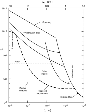
Figure 2: Strength of the modulus force relative to gravity ($\alpha^{2}$) versus its Compton wavelength ($\lambda$).

In fig. 2 we depict the actual information from previous, present and upcoming experiments [21]. The vertical axis is the strength, $\alpha^{2}$, of the force relative to gravity; the horizontal axis is the Compton wavelength of the exchanged particle; the upper scale shows the corresponding value of the supersymmetry breaking scale (large radius or string scale) in TeV. The solid lines indicate the present limits from the experiments indicated. The excluded regions lie above these solid lines. Measuring gravitational strength forces at such short distances is quite challenging. The most important background is the Van der Walls force which becomes equal to the gravitational force between two atoms when they are about 100 microns apart. Since the Van der Walls force falls off as the 7th power of the distance, it rapidly becomes negligible compared to gravity at distances exceeding 100 $\mu$m. The dashed thick line gives the expected sensitivity of the present and upcoming experiments, which will improve the actual limits by roughly two orders of magnitude and –at the very least– they will, for the first time, measure gravity to a precision of 1% at distances of $\sim$ 100 $\mu$m.

References

References

- [1] M. Green, J. Schwarz and E. Witten, Superstring Theory, Cambridge University Press, 1987; J. Polchinski, String Theory, Cambridge University Press, Cambridge, 1998.
- [2] For recent reviews, see A. Sen, hep-th/9802051, I. Antoniadis and G. Ovarlez, hep-th/9906108.
- [3] I. Antoniadis, Phys. Lett. B 246, 377 (1990).
- [4] L. Dixon, V. Kaplunovsky and J. Louis, Nucl. Phys. B 355, 649 (1991); I. Antoniadis, K. Narain and T. Taylor, Phys. Lett. B 267, 37 (1991).
- [5] I. Antoniadis, C. Bachas, D. Lewellen and T. Tomaras, Phys. Lett. B 207, 441 (1988).
- [6] C. Kounnas and M. Porrati, Nucl. Phys. B 310, 355 (1988); S. Ferrara, C. Kounnas, M. Porrati and F. Zwirner, Nucl. Phys. B 318, 75 (1989); E. Kiritsis and C. Kounnas, Nucl. Phys. B 503, 117 (1997).
- [7] T. Taylor and G. Veneziano, Phys. Lett. B 212, 147 (1988).
- [8] I. Antoniadis and B. Pioline, Nucl. Phys. B 550, 41 (1999), hep-th/9902055.
- [9] E. Witten, Proceedings of Strings 95, hep-th/9507121; A. Strominger, Phys. Lett. B 383, 44 (1996), hep-th/9512059;
- [10] N. Seiberg, Phys. Lett. B 390, 169 (1997), hep-th/9609161.
- [11] E. Witten, Nucl. Phys. B 471, 135 (1996), hep-th/9602070.
- [12] J.D. Lykken, Phys. Rev. D 54, 3693 (1996), hep-th/9603133.
- [13] N. Arkani-Hamed, S. Dimopoulos and G. Dvali, Phys. Lett. B 429, 263 (1998), hep-ph/9803315.
- [14] I. Antoniadis, N. Arkani-Hamed, S. Dimopoulos and G. Dvali, Phys. Lett. B 436, 263 (1998), hep-ph/9804398.
- [15] I. Antoniadis and C. Bachas, Phys. Lett. B 450, 83 (1999), hep-th/9812093.
- [16] P. Hořava and E. Witten, Nucl. Phys. B 460, 506 (1996), hep-th/9510209.
- [17] E. Caceres, V.S. Kaplunovsky and I.M. Mandelberg, Nucl. Phys. B 493, 73 (1997), hep-th/9606036.
- [18] J. Polchinski and E. Witten, Nucl. Phys. B 460, 525 (1996), hep-th/9510169.
- [19] G. Shiu and S.-H.H. Tye, Phys. Rev. D 58, 106007 (1998), hep-th/9805157; Z. Kakushadze and S.-H.H. Tye, Nucl. Phys. B 548, 180 (1999), hep-th/9809147; L.E. Ibáñez, C. Muñoz and S. Rigolin, hep-ph/9812397.
- [20] N. Arkani-Hamed, S. Dimopoulos and G. Dvali, Phys. Rev. D 59, 086004 (1999), hep-ph/9807344; S. Nussinov and R. Shrock, Phys. Rev. D 59, 105002 (1999), hep-ph/9811323; S. Cullen and M. Perelstein, Phys. Rev. Lett. 83, 268 (1999), hep-ph/9903422; L.J. Hall and D. Smith, hep-ph/9904267.
- [21] See for instance: J.C. Long, H.W. Chan and J.C. Price, Nucl. Phys. B 539, 23 (1999), hep-ph/9805217.
- [22] L.E. Ibáñez, Proceedings of Strings 99.
- [23] K. Benakli, hep-ph/9809582; C.P. Burgess, L.E. Ibáñez and F. Quevedo, Phys. Lett. B 447, 257 (1999).
- [24] I. Antoniadis and M. Quirós, Phys. Lett. B 392, 61 (1997), hep-th/9609209.
- [25] C.M. Hull and P.K. Townsend, Nucl. Phys. B 438, 109 (1995), hep-th/9410167 and Nucl. Phys. B 451, 525 (1995), hep-th/9505073; E. Witten, Nucl. Phys. B 443, 85 (1995), hep-th/9503124.
- [26] For a recent review, see P. Mayr, hep-th/9904115.
- [27] S. Katz and C. Vafa, Nucl. Phys. B 497, 146 (1997), hep-th/9606086; for a recent review, see P. Mayr, Fortsch. Phys. 47, 39 (1998), hep-th/9807096.
- [28] For a recent review, see N.A. Obers and B. Pioline, Phys. Rep. 318, 113 (1999), hep-th/9809039.
- [29] I. Antoniadis and K. Benakli, Phys. Lett. B 326, 69 (1994), hep-th/9310151.
- [30] V.A. Kostelecky and S. Samuel, Phys. Lett. B 270, 21 (1991); P. Nath and M. Yamaguchi, hep-ph/9902323 and hep-ph/9903298; W.J. Marciano, hep-ph/9902332 and hep-ph/9903451; M. Masip and A. Pomarol, hep-ph/9902467.
- [31] I. Antoniadis, K. Benakli and M. Quirós, Phys. Lett. B 331, 313 (1994), hep-ph/9403290 and Phys. Lett. B 460, 176 (1999), hep-ph/9905311; P. Nath, Y. Yamada and M. Yamaguchi, hep-ph/9905415; T.G. Rizzo and J.D. Wells, hep-ph/9906234; A. Strumia, hep-ph/9906266.
- [32] See for instance: G.F. Giudice, R. Rattazzi and J.D. Wells, Nucl. Phys. B 544, 3 (1999), hep-th/9811292; E.A. Mirabelli, M. Perelstein and M.E. Peskin, Phys. Rev. Lett. 82, 2236 (1999), hep-ph/9811337; T. Han, J. Lykken and R.-J. Zhang, Phys. Rev. D 59, 105006 (1999), hep-ph/9811350; J.L. Hewett, Phys. Rev. Lett. 82, 4765 (1999), hep-ph/9811356; T.G. Rizzo, Phys. Rev. D 59, 115010 (1999), hep-ph/9901209, Phys. Rev. D 60, 075001 (1999), hep-ph/9903475 and hep-ph/9904380; P. Mathews, S. Raychaudhuri and K. Sridhar, Phys. Lett. B 450, 343 (1999), hep-ph/9811501 and hep-ph/9904232; G. Shiu, R. Shrock and S.-H.H. Tye, Phys. Lett. B 458, 274 (1999), hep-ph/9904262; E. Halyo, hep-ph/9904432; M. Besancon, hep-ph/9909364.
- [33] C. Bachas, JHEP 9811, 23 (1998), hep-ph/9807415.
- [34] See also G. Dvali, Phys. Lett. B 459, 489 (1999), hep-ph/9905204.
- [35] K.R. Dienes, E. Dudas and T. Gherghetta, Phys. Lett. B 436, 55 (1998), hep-ph/9803466 and Nucl. Phys. B 537, 47 (1999), hep-ph/9806292; D. Ghilencea and G.G. Ross, Phys. Lett. B 442, 165 (1998); Z. Kakushadze, Nucl. Phys. B 548, 205 (1999), hep-th/9811193; A. Delgado and M. Quirós, hep-ph/9903400; P. Frampton and A. Rasin, Phys. Lett. B 460, 313 (1999), hep-ph/9903479; A. Pérez-Lorenzana and R.N. Mohapatra, hep-ph/9904504; Z. Kakushadze and T.R. Taylor, hep-th/9905137.
- [36] I. Antoniadis, C. Bachas and E. Dudas, hep-th/9906039.
- [37] N. Arkani-Hamed, S. Dimopoulos and J. March-Russell, hep-th/9908146.
- [38] S. Kachru and E. Silverstein, JHEP 11, 1 (1998), hep-th/9810129; J. Harvey, Phys. Rev. D 59, 26002 (1999); R. Blumenhagen and L. Görlich, hep-th/9812158; C. Angelantonj, I. Antoniadis and K. Foerger, Nucl. Phys. B 555, 116 (1999), hep-th/9904092.
- [39] I. Antoniadis, E. Dudas and A. Sagnotti, hep-th/9908023; G. Aldazabal and A.M. Uranga, hep-th/9908072.
- [40] C. Bachas, hep-th/9503030; J.G. Russo and A.A. Tseytlin, Nucl. Phys. B 461, 131 (1996).
- [41] For recent reviews, see A. Sen, hep-th/9904207; A. Lerda and R. Russo, hep-th/9905006.
- [42] I. Antoniadis, E. Dudas and A. Sagnotti, Nucl. Phys. B 544, 469 (1999); I. Antoniadis, G. D’Appollonio, E. Dudas and A. Sagnotti, Nucl. Phys. B 553, 133 (99), hep-th/9812118 and hep-th/9907184.
- [43] I. Antoniadis, S. Dimopoulos and G. Dvali, Nucl. Phys. B 516, 70 (1998), hep-ph/9710204.
- [44] I. Antoniadis, C. Muñoz and M. Quirós, Nucl. Phys. B 397, 515 (1993); A. Pomarol and M. Quirós, Phys. Lett. B 438, 225 (1998), hep-ph/9806263; I. Antoniadis, S. Dimopoulos, A. Pomarol and M. Quirós, Nucl. Phys. B 544, 503 (1999), hep-ph/9810410; A. Delgado, A. Pomarol and M. Quirós, hep-ph/9812489.
- [45] S. Ferrara, C. Kounnas and F. Zwirner, Nucl. Phys. B 429, 589 (1994).
- [46] T.R. Taylor and G. Veneziano, Phys. Lett. B 213, 450 (1988).