Preprint CERN TH 99–275, September 6, 1999
                                            Preprint NBI–HE–99–1
Phase Transition Couplings in the Higgsed Monopole Model

Abstract

Using a one-loop approximation for the effective potential in the Higgs model of electrodynamics for a charged scalar field, we argue for the existence of a triple point for the renormalized (running) values of the selfinteraction $\lambda$ and the ”charge” $g$ given by $(\lambda_{run},g^{2})=(-\frac{10}{9}\pi^{2},\frac{4}{3}\sqrt{\frac{5}{3}}{\pi^{2}})\approx(-11,17)$. Considering the beta-function as a typical quantity we estimate that the one-loop approximation is valid with accuracy of deviations not more than 30% in the region of the parameters: $0.2\stackrel{{\scriptstyle<}}{{\sim}}{\large\alpha,\tilde{\alpha}}\stackrel{{\scriptstyle<}}{{\sim}}1.35.$ The phase diagram given in the present paper corresponds to the above-mentioned region of $\alpha,\;\tilde{\alpha}$. Under the point of view that the Higgs particle is a monopole with a magnetic charge $g$, the obtained electric fine structure constant turns out to be $\alpha_{crit}\approx{0.18_{5}}$ by the Dirac relation. This value is very close to the $\alpha_{crit}^{lat}\approx{0.20}$ which in a $U(1)$ lattice gauge theory corresponds to the phase transition between the ”Coulomb” and confinement phases. Such a result is very encouraging for the idea of an approximate ”universality” (regularization independence) of gauge couplings at the phase transition point. This idea was suggested by the authors in their earlier papers.

PACS: 11.15.Ha; 12.38.Aw; 12.38.Ge; 14.80.Hv
Keywords: gauge theory, phase transition, monopole, lattice, one-loop approximation

Corresponding author
(temporary address from 01.08.1999 to 01.08.2000):
Prof.H.B.Nielsen,
Theory Division
CERN
CH 1211 Geneva 23
Switzerland
Telephone: +41 227678757
E-mail: Holger.Bech.Nielsen@cern.ch

1 Introduction

The Standard Model (SM) describes well all experimental results known today. Most efforts to explain the SM are devoted to Grand Unification Theories (GUTs). The supersymmetric extension of the SM consists of taking the SM and adding the corresponding supersymmetric partners [1]. The precision of the LEP data allows us to extrapolate three running constants $\alpha_{i}(\mu)$ of the SM (i=1,2,3 for U(1), SU(2), SU(3) groups) to high energies with small errors and we are able to perform the consistency checks of GUTs.

In the SM based on the group

$$SMG=SU(3)_{c}\otimes SU(2)_{L}\otimes U(1)_{Y}$$ (1)

the usual definitions of the coupling constants are used:

$$\alpha_{1}=\frac{5}{3}\frac{\alpha}{\cos^{2}\theta_{\overline{MS}}},\quad\alpha_{2}=\frac{\alpha}{\sin^{2}\theta_{\overline{MS}}},\quad\alpha_{3}\equiv\alpha_{S}=\frac{g^{2}_{S}}{4\pi},$$ (2)

where $\alpha$ and $\alpha_{s}$ are the electromagnetic and strong fine structure constants, respectively. All of these couplings, as well as the weak angle, are defined here in the Modified Minimal Subtraction scheme $(\overline{MS})$ (see Reviews of Particle Physics). Using experimentally given parameters and the renormalization group equations (RGE), it is possible to extrapolate the experimental values of three inverse running constants $\alpha_{i}^{-1}(\mu)$ to the Planck scale:

$$\mu_{Pl}=1.22\cdot{10}^{19}\;GeV.$$ (3)

The comparison of the evolutions of the inverses of the running coupling constants in the Minimal Standard Model (MSM) (with one Higgs doublet) and in the Minimal Supersymmetric Standard Model (MSSM) (with two Higgs doublets) shows the possibility of the existence of the grand unification point at $\mu_{GUT}\sim 10^{16}$ GeV only in the case of the MSSM (see Ref.[2]). But the absence of supersymmetric particle production at current accelerators and additional constraints arising from limits on the contributions of virtual supersymmetric particle exchange in a variety of the SM processes indicate that at present there are no unambiguous experimental results requiring the existence of supersymmetry.

Scenarios based on the Anti-Grand Unification Theory (AGUT) was developed in Refs.[3]-[14] as a realistic alternative to SUSY GUTs (see Ref.[13]). AGUT suggests the following assumption: supersymmetry does not exist up to the Planck scale. There is no new physics (new particles, superpartners) up to around an order of magnitude under this scale, and the renormalization group extrapolation of experimentally determined couplings to the Planck scale is contingent to not encountering new particles.

AGUT suggests that at the Planck scale $\mu_{Pl}$, considered as a fundamental scale, there exists the more fundamental gauge group $G$, containing $N_{gen}$ copies of the Standard Model group $SMG$:

$$G=SMG_{1}\otimes SMG_{2}\otimes\ldots\otimes SMG_{N_{gen}}\equiv(SMG)^{N_{gen}},$$ (4)

where the integer $N_{gen}$ designates the number of quark and lepton generations.

SMG by definition is the following factor group:

$$SMG=S(U(2)\times U(3))=\frac{U(1)\times SU(2)\times SU(3)}{\{{(2\pi,-1^{2\times 2},e^{i2\pi/3}1^{3\times 3})}^{n}|n\in Z\}}.$$ (5)

If $N_{gen}=3$, then the fundamental gauge group G is:

$$G=(SMG)^{3}=SMG_{1}\otimes SMG_{2}\otimes SMG_{3},$$ (6)

or the generalized G:

$$G={(SMG)}^{3}\otimes U(1)_{f}$$ (7)

which follows from the fitting of fermion masses (see Ref.[11]). The group $G={(SMG)}^{3}\otimes U(1)_{f}$ is a maximal gauge transforming (nontrivially) the 45 Weyl fermions of the SM (which it extends) without unifying any of the irreducible representations of the group of the latter. Anomalies are absent in this theory.

The AGUT approach was used in conjunction with the Multiple Point Principle (MPP) proposed several years ago by D.L.Bennett and H.B.Nielsen [7]-[9]. Another name for the same principle is the ”Maximally Degenerate Vacuum Principle” (MDVP). According to this principle, Nature seeks a special point – the multiple critical point (MCP) – where the group $G$ undergoes spontaneous breakdown to the diagonal subgroup:

$$G\to G_{diag.subgr.}=\left\{g,g,g\parallel g\in SMG\right\}$$ (8)

which is identified with the usual (low-energy) group SMG.

The idea of the MPP has its origin in the lattice investigations of gauge theories. In particular, Monte Carlo simulations on the lattice of U(1)–, SU(2)– and SU(3)– gauge theories indicate the existence of a triple point. Using theoretical corrections to the Monte Carlo results on the lattice, it is possible to make slightly more accurate predictions of AGUT for the SM fine-structure constants. The MPP assumes that the SM gauge couplings do not unify and predicts the following values of the fine structure constants at the Planck scale in terms of the phase transition (critical) couplings taken from the lattice gauge theories:

$$\alpha_{i}(\mu_{Pl})=\frac{\alpha_{i}^{crit}}{N_{gen}}=\frac{\alpha_{i}^{crit}}{3}$$ (9)

for $i=2,3$ and

$$\alpha_{1}(\mu_{Pl})=\frac{\alpha_{1}^{crit}}{{\frac{1}{2}}N_{gen}(N_{gen}+1)}=\frac{\alpha_{1}^{crit}}{6}$$ (10)

for U(1).

This means that at the Planck scale the fine structure constants $\alpha_{Y}\equiv\frac{3}{5}\alpha_{1}$, $\alpha_{2}$ and $\alpha_{3},$ as chosen by Nature, are just the ones corresponding to the Multiple Critical Point (MCP) which is a point where all action parameter (coupling) values meet in the phase diagram of the regularized Yang-Mills $(SMG)^{3}$ – gauge theory. Nature chooses coupling constant values such that a number of vacuum states have the same energy density. Then all (or just many) numbers of phases convene at the MCP and different vacua are degenerate.

The extrapolation of the experimental values of the inverses $\alpha^{-1}_{Y,2,3}(\mu)$ to the Planck scale $\mu_{Pl}$ by the renormalization group formulae (under the assumption of a ”desert” in doing the extrapolation with one Higgs doublet) leads to the following result:

$$\alpha^{-1}_{Y}(\mu_{Pl})=55.5;\quad\alpha^{-1}_{2}(\mu_{Pl})=49.5;\quad\alpha^{-1}_{3}(\mu_{Pl})=54.$$ (11)

Using the AGUT prediction given by Eq.(10) and the first value of Eq.(11) we have the following AGUT estimation for the U(1) fine structure constant at the phase transition point:

$$\alpha_{crit}^{-1}\sim 9.$$ (12)

Previously we have also speculated and made supportive calculations [12]-[14] that the dependence of the cut-off procedure is rather small: phase transition coupling constants would not differ very much using one or the other regularization. So we hope that there exists what one might call ”an approximate universality”.

For the second-order phase transitions the exact universality would be expected, but for the first-order phase transitions, which we really hope for in the mentioned works, such an exact universality would be quite unexpected. However, we still believe that an approximate one really exists. Indeed, the main purpose of the present article is to calculate the phase transition couplings and to confirm this desired ”approximate universality”. The point is that the cut-off considered in the previous works for MPP coupling calculations was connected with the existence of artifact monopoles in the theory: there are artifact monopoles in the lattice gauge theory and also in the Wilson loop action model which we proposed [12].

The idea now is: instead of using the cut-off, we introduce physically existing monopoles as fundamental fields into the theory. Then one may not use the cut-off, but can rather think of any cut-off, although essentially it should no longer matter. In other words, we consider a theory with monopoles and look for a, or rather several, phase transitions connected with the monopoles forming a condensate in the vacuum. Writing such a monopole theory in the dual field formulation, we deal with the usual Higgs model.

Below, using the Zwanziger formalism [15]–[17] for the dual Abelian gauge theory describing the system with two (dual and non-dual) gauge fields and both magnetic and electric charges (see Section 3), we confirm in Section 6 a rather simple expression for the effective potential in the one-loop approximation which was obtained for the Higgsed scalar electrodynamics in Ref.[18] (see also Ref.[19]), and investigate the phase structure of the Higgs model. But now the Higgs scalar field is identified with the monopole field having magnetic charge $g$. This means that the electric charge $e$ is connected to the formal charge $g$ of this Higgs field via the Dirac relation:

$$eg=2\pi,$$ (13)

Then we can define the electric and magnetic fine structure constants:

$$\alpha=e^{2}/4\pi=\pi/g^{2},\quad\quad\tilde{\alpha}=g^{2}/4\pi=\pi/e^{2}.$$ (14)

In Section 5 we investigate the renormalization group equations for $\alpha$ and $\tilde{\alpha}$ in the case of the existence of both charges and confirm the Dirac relation for all renormalized effective coupling constants. Thus, for the arbitrary scale we have the following relation:

$$\alpha\tilde{\alpha}=\frac{1}{4}$$ (15)

which is used in Section 7 for the calculation of the critical (phase transition) fine structure constants.

It seems that the region of parameters $\alpha$ and $\tilde{\alpha}$ near the phase transition point ($\alpha_{crit}\approx{0.2}$ and ${\tilde{\alpha}}_{crit}\approx 1.25$) obtained in the lattice investigations [21]-[23] of the U(1) gauge theory allows us to consider the perturbation theory in both electric and magnetic sectors with accuracy of deviations $\stackrel{{\scriptstyle<}}{{\sim}}30\%$ (see Section 5).

In the present paper we aim to give the explanation of lattice results and, what is more important, to show that the first-order phase transition arises in the Higgsed monopole model already on the level of the ”improved” one-loop approximation (see Section 7), which describes the phase transition found on the lattice with acceptable accuracy. Thus, if the lattice phase transition coupling roughly coincides with our Coleman–Weinberg model it cannot depend much on lattice details. As it will be shown below, such a perturbation theory reproduces the lattice result. Thus we get the suggested ”approximate universality” even for first-order phase transitions.

2 Phase Transition Coupling in Lattice U(1) Gauge Theory (Compact QED)

As was mentioned in Section 1, the idea of the MPP is based on the lattice investigations of gauge theories. In particular, Monte Carlo simulations of the U(1) gauge theory described by the following lattice action:

$$S=\sum_{\Box}[\beta\cos{\Theta(\Box)}+\gamma\cos{2\Theta(\Box)}]$$ (16)

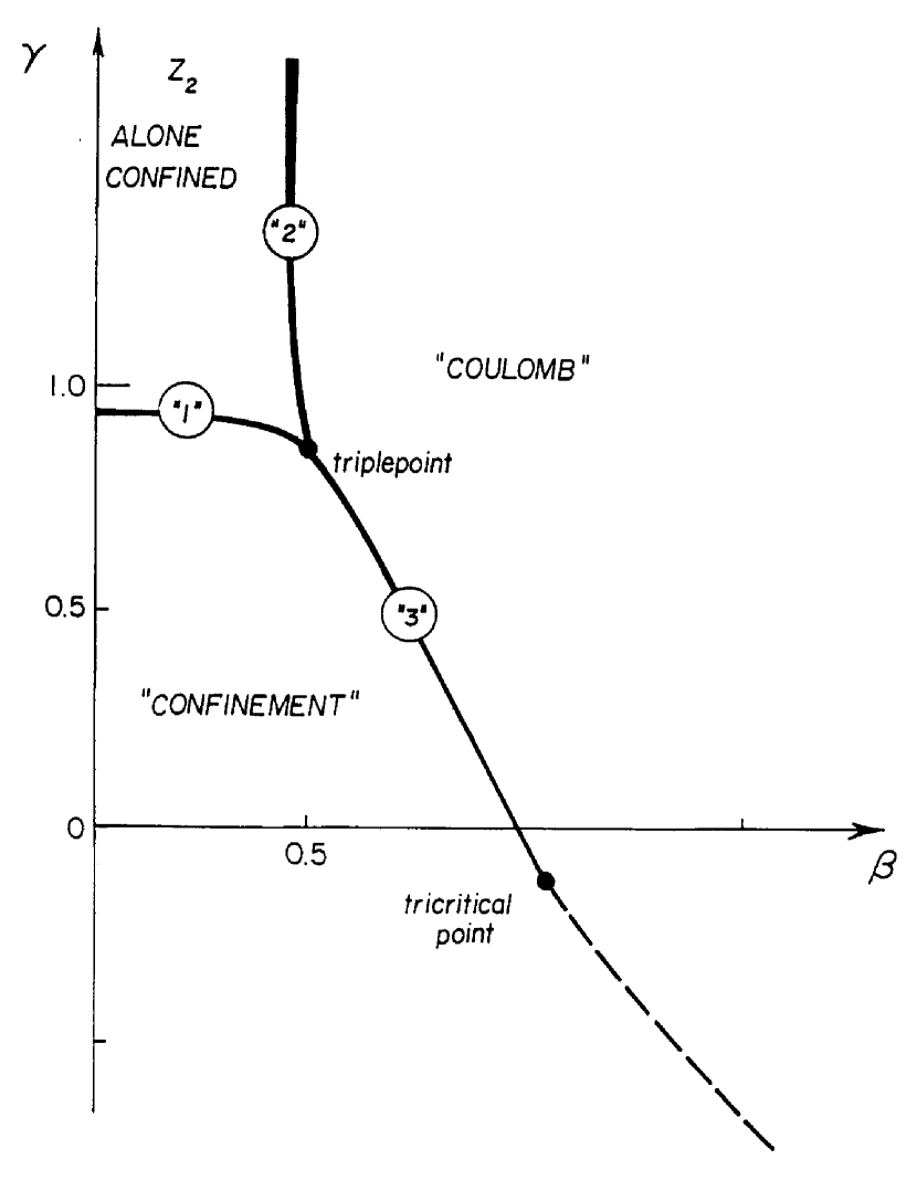
Fig. 1: The phase diagram for $U(1)$ when the two-parameter action is used. This type of action makes it possible to provoke the confinement $Z_{2}$ (or $Z_{3}$) alone.

(here $\Theta(\Box)$ is the plaquette variable) indicate the existence of the triple point [21]-[23] on the phase diagram shown in Fig.1. From this triple point emanate three phase borders: the phase border ”1” separates the totally confining phase from the phase where only the discrete subgroup $Z_{2}$ is confined; the phase border ”2” separates the latter phase from the totally Coulomb-like phase; and the phase border ”3” separates the totally confining and totally Coulomb-like phases.

In the speculative ideas which were proposed to provide a mechanism for the MPP degeneracy of vacua in nature, one typically gets the prediction that the phase transition is first order [7]-[9] - for instance, if the world is in a state analogous to a microcanonical ensemble leading to a mixture of phases.

In the Higgs monopole model considered in this paper you find a priori formally first-order transitions, but it is possible to give some estimates showing that this may not always be expected to be true at the end. We shall leave this problem for the next paper.

In search for a lattice formulation of QED with a second order phase transition, the simple Wilson action was generalized to Eq.(16) by including a double charge term with coupling $\gamma$ [20] in the expectation that the phase transition would be driven towards second-order at sufficiently small negative values of $\gamma$.

The recent lattice simulations of compact QED [23]-[31] have still not succeeded in agreement when they clarify the order of the phase transition near $\beta=1$. However, simulations on the hyper-torus, up to $\gamma=$ - 0.4, revealed the reappearance of a double peak on large enough lattices [28]. In addition, for $\gamma$ between + 0.2 and - 0.4 the critical exponent $\nu$ has been found to decrease towards $\frac{1}{4}$ (which corresponds to the first-order phase transition [30]) with increasing lattice size for toroidal as well for spherical geometry. In some cases stabilization of the latent heat has been observed. Now we have rather strong indications that, at least in the region up to $\gamma=$ - 0.4, the phase transition is of first order.

Fig.1 represents this situation showing, the tricritical point at some negative value of the parameter $\gamma$. Of course, it remains desirable to check this result on still larger lattices.

In Ref.[21] the behaviour of the effective fine structure constant $\alpha(\beta)$ (here $\beta=1/e_{0}^{2}$, and $e_{0}$ is the bare electric charge) were investigated in the vicinity of the phase transition point for the case $\gamma=0$, and the following values of the fine structure constants at the phase transition point was obtained:

$$\alpha_{crit}^{lat}\approx{0.20},\quad{\tilde{\alpha}}_{crit}^{lat}\approx{1.25},\quad\quad\mbox{at}\quad\quad\beta_{crit}\approx{1.011}.$$ (17)

Considering the Villain lattice action which corresponds to the extended Wilson action (16) with $\gamma\approx{-\;0.22}$, the authors of Ref.[23] revised the values of the renormalized electrical coupling $\alpha$ obtained in Ref.[21] and presented :

$$\alpha^{lat}\approx{0.1836},\quad{\tilde{\alpha}}^{lat}\approx{1.36}\quad\\ \mbox{ in the vicinity of the phase transition point}.$$ (18)

The compact lattice QED is essentially related to the monopoles. The phase transition ”Coulomb - confinement” is known to be associated with the condensation of magnetic monopoles [23],[29],[32]-[34]. Monopole vacuum loops renormalize the fine structure constant $\alpha$ by an amount proportional to the susceptibility of the monopole gas [34]. The enhancement factor of this renormalization was estimated in Ref.[12]:

$$K=\frac{\alpha_{crit}(\mbox{Monte Carlo})}{\alpha_{crit}(\mbox{theory without monopoles})}\approx{1.66}.$$ (19)

The power law scaling behaviour of the monopole mass and condensate was observed in Ref.[23]. Using their results we have extracted the ratio of the monopole mass to the monopole condensate $\rho=<0|\Phi|0>$ ($\Phi$ is a monopole field) in the confinement phase, a little bit away from the phase transition point (but near to it):

$$\frac{m}{\rho}\approx{2.4}.$$ (20)

By this ”little bit away” we allude to the fact that $m/\rho$ varies rather little except for $\beta$ being shorter than $\Delta\beta\approx{0.04}$ away from $\beta_{crit}$. That is, the ratio (20) takes place in the slowly varying region when approaching the phase transition.

In the lattice gauge theory monopoles are not physical objects: they are lattice artifacts driven to infinite mass in the continuum limit.

Also in Ref.[12], instead of the lattice hypercubic regularization, we have considered rather new regularization using non-local Wilson loop action in the approximation of circular loops of radii $R\geq a$. It was shown that the critical fine structure constant is rather independent of the regularization method. Its value is given by the following expression:

$$\alpha_{crit}\approx{0.204},$$ (21)

in correspondence with the Monte Carlo simulation result (17),(18) on the lattice. Such a phase transition coupling ”universality” is needed too much for the fine structure constant predictions claimed from the MPP. But independently of the Multiple Point Model, the ”approximate universality” (if it takes place) is an important phenomenon for the phase transition in any gauge field theory.

3 The Zwanziger Formalism for the Abelian Gauge Theory with Electric and Magnetic Charges

In the lattice gauge theories and in the nonlocal Wilson loop model mentioned in Section 2, monopoles are artifacts of the regularization. Let us assume now a physically existing fundamental regulator. The new idea is to consider monopoles as fundamental fields. With the aim of confirming the universality of the critical couplings in this case, we have investigated for a phase transition the quantum field theory with electric and magnetic charges considering monopoles as Higgs scalar particles.

A version of the local field theory of electrically and magnetically charged particles is represented by Zwanziger formalism [15],[16] (see also [17]) which considers two potentials $A_{\mu}(x)$ and $B_{\mu}(x)$ describing one physical photon with two physical degrees of freedom. Now and below we call this theory QEMD (”quantum electromagnetodynamics”).

In QEMD the total field system of the gauge, electrically ($\Psi$) and magnetically ($\Phi$) charged fields is described by the partition function which has the following form in Euclidean space:

$$Z=\int[DA][DB][D\Phi][D\bar{\Phi}][D\Psi][D\bar{\Psi}]e^{-S}$$ (22)

where

$$S=S_{Zw}(A,B)+S_{gf}+S_{e}+S_{m}.$$ (23)

The Zwanziger action $S_{Zw}(A,B)$ is given by:

$$S_{Zw}(A,B)=\int d^{4}x[\frac{1}{2}{(n\cdot[\partial\wedge A])}^{2}+\frac{1}{2}{(n\cdot[\partial\wedge B])}^{2}+\\$$

$$+\frac{i}{2}(n\cdot[\partial\wedge A])(n\cdot{[\partial\wedge B]}^{*})-\frac{i}{2}(n\cdot[\partial\wedge B])(n\cdot{[\partial\wedge A]}^{*})],$$ (24)

where we have used the following designations:

$${[A\wedge B]}_{\mu\nu}=A_{\mu}B_{\nu}-A_{\nu}B_{\mu},\quad{(n\cdot[A\wedge B])}_{\mu}=n_{\nu}{(A\wedge B)}_{\nu\mu},\\$$

$$\quad{G}^{*}_{\mu\nu}=\frac{1}{2}\epsilon_{\mu\nu\lambda\rho}G_{\lambda\rho}.$$ (25)

The actions $S_{e}$ and $S_{m}$:

$$S_{e,m}=\int d^{4}xL_{e,m}(x)$$ (26)

describe, respectively, the electrically and magnetically charged matter fields, and $S_{gf}$ is the gauge-fixing action.

At the same time we present the generating functional with external sources $J_{\mu}^{(A)},J_{\mu}^{(B)},\eta$ and $\omega$:

$$Z[J^{(A)},J^{(B)},\eta,\omega]=$$

$$=\int[DA][DB][D\Phi][D\bar{\Phi}][D\Psi][D\bar{\Psi}]e^{-S+(J^{(A)},A)+(J^{(B)},B)+(\bar{\eta},\Phi)+(\bar{\Phi},\eta)+(\bar{\omega},\Psi)+(\bar{\Psi},\omega)}$$ (27)

where

$$(J,A)=\int d^{4}xJ_{\mu}(x)A_{\mu}(x),\quad\mbox{and}\quad(\bar{\eta},\Phi)=\int d^{4}x\bar{\eta}(x)\Phi(x),\quad\mbox{etc.}$$ (28)

Let us consider now the Lagrangian $L_{m}$ describing the Higgs scalar monopole field $\Phi(x)$ interacting with the dual gauge field $B_{\mu}(x)$:

$$L_{m}(x)=-\frac{1}{4}{(\partial\wedge B)}^{2}+\frac{1}{2}{|{\tilde{D}}_{\mu}\Phi|}^{2}+U(\Phi),$$ (29)

where

$${\tilde{D}}_{\mu}=\partial_{\mu}-igB_{\mu}$$ (30)

is a covariant derivative for the dual field;

$$U(\Phi)=\frac{1}{2}{\mu_{m}}^{2}{|\Phi|}^{2}+\frac{\lambda_{m}}{4}{|\Phi|}^{4}$$ (31)

is the Higgs potential for monopoles.

The complex scalar field:

$$\Phi=\phi+i\chi$$ (32)

contains Higgs and Goldstone boson fields $\phi(x)$ and $\chi(x)$, respectively.

Now we have a number of possibilities to describe electrically charged fields (below we give the Lagrangian expressions in Minkowski space). They can be:

a) fermions (electrons) described by the Dirac Lagrangian:

$$L_{e}=L_{e}^{(f)}=\bar{\Psi}{\gamma}_{\mu}(iD_{\mu}-\mu_{e})\Psi,$$ (33)

b) Klein–Gordon (complex) scalars:

$$L_{e}=L_{e}^{(s)}=\frac{1}{2}[{|D_{\mu}\Psi|}^{2}-{\mu_{e}}^{2}{|\Psi|}^{2}],$$ (34)

or c) Higgs scalars:

$$L_{e}=L_{e}^{(Hs)}=\frac{1}{2}{|D_{\mu}\Psi|}^{2}-U(|\Psi|)$$ (35)

where

$$D_{\mu}=\partial_{\mu}-ieA_{\mu},$$ (36)

and

$$U(|\Psi|)=\frac{1}{2}\mu_{e}^{2}{|\Psi|}^{2}+\frac{\lambda_{e}}{4}{|\Psi|}^{4}$$ (37)

is the Higgs potential for the electrically charged field.

Using the generating functional (27) it is not difficult to calculate the propagators of the fields considered in this model.

Three ”bare” propagators of the gauge fields $A_{\mu}$ and $B_{\mu}$:

$$Q_{\mu\nu}^{0(A)}=<A_{\mu}A_{\nu}>=\frac{\delta^{2}Z[J^{(A)},J^{(B)},\eta,\omega]}{\delta J_{\mu}^{(A)}\delta J_{\nu}^{(A)}},\quad$$

$$Q_{\mu\nu}^{0(B)}=<B_{\mu}B_{\nu}>=\frac{\delta^{2}Z[J^{(A)},J^{(B)}\eta,\omega]}{\delta J_{\mu}^{(B)}\delta J_{\nu}^{(B)}},$$

$$Q_{\mu\nu}^{0(AB)}=<A_{\mu}B_{\nu}>=\frac{\delta^{2}Z[J^{(A)},J^{(B)},\eta,\omega]}{\delta J_{\mu}^{(A)}\delta J_{\nu}^{(B)}}$$ (38)

were calculated by the authors of Ref.[17] in the momentum space:

$$Q_{\mu\nu}^{0(A,B)}(q)=\frac{1}{q^{2}}\bigl{(}\delta_{\mu\nu}+\frac{q^{2}+{M_{A,B}}^{2}}{M^{2}_{A,B}}\frac{q_{\mu}q_{\nu}}{{(n\cdot q)}^{2}}-\frac{1}{(n\cdot q)}(q_{\mu}n_{\nu}+q_{\nu}n_{\mu})\bigr{)},$$ (39)

and

$$Q_{\mu\nu}^{0(AB)}=\frac{i}{q^{2}}\epsilon_{\mu\nu\rho\sigma}\frac{q_{\rho}n_{\sigma}}{(n\cdot q)}.$$ (40)

The parameters $M_{(A,B)}$ are connected with the gauge. The gauge-fixed action chosen in Ref.[17]:

$$S_{gf}=\int d^{4}x[\frac{M^{2}_{A}}{2}{(nA)}^{2}+\frac{M^{2}_{B}}{2}{(nB)}^{2}]$$ (41)

has no ghosts.

All Lagrangians (33)–(35) have the interaction term $j_{\mu}^{e}A_{\mu}$ where $j_{\mu}^{e}$ is the electric current. The interactions in the Lagrangian (29) are given by $j_{\mu}^{m}B_{\mu}$ (here $j_{\mu}^{m}$ is the magnetic current) as well as by the ”seagull” term $g^{2}B_{\mu}B_{\mu}{\bar{\Phi}}\Phi$. The equivalent seagull terms are present in the Lagrangians (34) and (35). The interaction between the electric and magnetic charges is carried out via the propagator $Q_{\mu\nu}^{(AB)}$.

4 Dual Symmetry

Duality is a symmetry appearing in free electromagnetism as invariance of the free (static) Maxwell equations:

$$\bf{\Delta}\cdot\vec{\bf B}=0,\quad\quad\bf{\Delta}\times\vec{\bf E}=0,$$ (42)

$$\bf{\Delta}\cdot\vec{\bf E}=0,\quad\quad\bf{\Delta}\times\vec{\bf B}=0,$$ (43)

under the interchange of electric and magnetic fields:

$$\vec{\bf E}\to\vec{\bf B},\quad\quad\vec{\bf B}\to-\vec{\bf E}.$$ (44)

Letting

$$F=\partial\wedge A=-(\partial\wedge B)^{*},$$ (45)

$$F^{*}=\partial\wedge B=(\partial\wedge A)^{*},$$ (46)

it is easy to see that the following equations:

$$\partial_{\lambda}F_{\lambda\mu}=0$$ (47)

with the Bianchi identity:

$$\partial_{\lambda}F_{\lambda\mu}^{*}=0,$$ (48)

equivalent to Eqs.(42), (43) are invariant under the Hodge star operation on the field tensor:

$$F_{\mu\nu}^{*}=\frac{1}{2}\epsilon_{\mu\nu\rho\sigma}F_{\rho\sigma}$$ (49)

(here $F^{**}=-F$).

This Hodge star duality applied to the free Zwanziger Lagrangian (24) leads to its invariance under the following duality transformations:

$$F\leftrightarrow F^{*},\quad\quad(\partial\wedge A)\leftrightarrow(\partial\wedge B),\quad\quad(\partial\wedge A)^{*}\leftrightarrow-(\partial\wedge B)^{*}.$$ (50)

Introducing the interacting Maxwell equations:

$$\partial_{\lambda}F_{\lambda\mu}=j_{\mu}^{e},$$ (51)

$$\partial_{\lambda}F_{\lambda\mu}^{*}=j_{\mu}^{m},$$ (52)

with the local conservation laws for electric and magnetic charge:

$$\partial_{\mu}j_{\mu}^{e,m}=0,$$ (53)

we immediately see the invariance of these equations under the exchange of the electric and magnetic fields (Hodge star duality) provided that at the same time the electric and magnetic charges and currents (and masses of the electrically and magnetically charged particles if they are different) are also interchanged:

$$e\leftrightarrow g,\quad\quad j_{\mu}^{e}\leftrightarrow j_{\mu}^{m}$$ (54)

(and $\mu_{e}\leftrightarrow\mu_{m}$). We shall consider this symmetry as the generalized duality.

The quantum field theory with electric $e_{i}$ and magnetic $g_{i}$ charges is selfconsistent if both charges are quantized according to the famous Dirac relation [38]:

$$e_{i}g_{j}=2\pi n_{ij}$$ (55)

when $n_{ij}$ is an integer. Considering $n_{ij}=1$ in Eq.(55) we obtain the Dirac quantization condition (13) in terms of the elementary electric and magnetic charges.

If the fundamental electric charge $e$ is so small that it corresponds to the perturbative electric theory, then magnetic charges are large and correspond to the strongly interacting magnetic theory, and vice versa. But below we consider some small region of $e,g$ values (we hope that it exists) which allows us to employ the perturbation theory in both the electric and magnetic sectors.

When nontrivial dyons – particles with both electric and magnetic charges simultaneously – are present, then the analogue of the Dirac relation becomes a bit more complicated and it then reads:

$$e_{i}g_{j}-e_{j}g_{i}=2\pi n_{ij}$$ (56)

which is duality invariant (see for example the review [39] and the references there).

The relation (56) has the name of the Dirac–Schwinger–Zwanziger [15],[38],[40] quantization condition. But the dyon theory is not exploited in this paper.

Now we are ready to calculate the effective potential. But first we prefer to consider the Dirac relation and the renormalization group equations for the renormalized electric and magnetic fine structure constants.

5 Renormalization Group Equations for the Electric and Magnetic Fine Structure Constants. The Dirac Relation

It is well known that in the absence of monopoles, the Gell-Mann–Low equation has the following form:

$$\frac{\mbox{d}(\log\alpha(p))}{\mbox{d}t}=\beta(\alpha(p))$$ (57)

where

$$t=\log(p^{2}/M^{2}),$$ (58)

$p$ is a 4-momentum and $\alpha=e^{2}/4\pi$.

The Gell-Mann–Low function $\beta(\alpha)$ depends on the Lagrangian describing theory. As the was first shown in Refs.[35], at sufficiently small charge ($\alpha<1$) the $\beta-$function is given by series over $\alpha/4\pi$:

$$\beta(\alpha)=\beta_{2}(\frac{\alpha}{4\pi})+\beta_{4}{(\frac{\alpha}{4\pi})}^{2}+...$$ (59)

The first two terms of this series were calculated in a QED long time ago in Refs.[35],[36]. The following result was obtained in the framework of the perturbation theory (in the one- and two-loop approximations):

a)

$$\beta_{2}=\frac{4}{3}\quad\mbox{and}\quad\beta_{4}=4\quad-\quad\mbox{for fermion (electron) loops}$$ (60)

and

b)

$$\beta_{2}=\frac{1}{3}\quad\mbox{and}\quad\beta_{4}=1\quad-\quad\mbox{for scalar particle loops}.$$ (61)

This result means that for both cases a) and b) the $\beta$-function can be represented by the following series arising from Eq.(59):

$$\beta(\alpha)=\beta_{2}(\frac{\alpha}{4\pi})(1+3\frac{\alpha}{4\pi}+...)$$ (62)

and we are able to exploit the one-loop approximation (given by the first term of Eqs.(59) and (62)) up to $\alpha\sim 1$ (with accuracy $\approx 25\%$ for the $\alpha\simeq 1$).

It is necessary to comment that three- and higher loop approximations depend on the renormalization scheme. We do not discuss this problem in the present paper.

The Dirac relation and the renormalization group equations (RGE) for the electric and magnetic fine structure constants $\alpha$ and $\tilde{\alpha}$ were investigated in detail by the authors in the recent paper [37] where the same Zwanziger formalism was developed for QEMD. The following result was obtained:

$$\frac{d\log\alpha(p)}{dt}=-\frac{d\log{\tilde{\alpha}}(p)}{dt}=\beta^{(e)}(\alpha)-\beta^{(m)}(\tilde{\alpha}).$$ (63)

It is easy to see that these RG-equations are in accordance with the Dirac relation (15) and with the generalized duality considered in Section 4.

In Eq.(63) the functions $\beta^{(e)}(\alpha)$ and $\beta^{(m)}(\tilde{\alpha})$ are described by the contributions of the electrically and magnetically charged particle loops, respectively. Their analytical expressions coincide with the usual well-known $\beta$–functions of QED given by Eq.(59), at least on the level of the two-loop approximation.

It is necessary to give some explanations how the result (63) was obtained.

J.Schwinger had shown [40] that the Dirac relation (13) is valid not only for the ”bare” $e_{0}$ and $g_{0}$, but also for the renormalized effective charges $e$ and $g$:

$$eg=e_{0}g_{0}=2\pi.$$ (64)

Eq.(64) confirms the equality:

$$\frac{d\log\alpha(p)}{dt}=-\frac{d\log\tilde{\alpha}(p)}{dt}$$ (65)

and means that the Dirac relation is valid for all scales, e.g. for all $t$ in RGE (63).

If the derivative ${d\log\alpha(p)}/dt$ in QEMD is also only a function of the effective fine structure constants as in the Gell-Mann–Low theory then we can write, in general, the following RGE:

$$\frac{d\log\alpha(p)}{dt}=\beta_{1}(\alpha)+\beta_{2}(\tilde{\alpha})+C,$$ (66)

$$\frac{d\log{\tilde{\alpha}}(p)}{dt}={\tilde{\beta}}_{1}(\alpha)+{\tilde{\beta}}_{2}(\tilde{\alpha})+\tilde{C}.$$ (67)

In Eqs.(66),(67) the terms containing the product $\alpha\tilde{\alpha}$ are absent due to the Dirac relation (15). Applying to Eqs.(66),(67) the duality symmetry (the invariance under the interchange $\alpha\leftrightarrow\tilde{\alpha}$) and using Eq.(65) (which is the consequence of the Dirac relation) it is not difficult to establish the following relations:

$$\beta_{1}(\alpha)=-\beta_{2}(\alpha)=-{\tilde{\beta}}_{1}(\alpha)={\tilde{\beta}}_{2}(\alpha),\\$$

$$C=\tilde{C}=0.$$ (68)

This result confirms the validity of RGE (63) with the function $\beta^{(m)}(\tilde{\alpha})$ given by the same analytical expressions as the $\beta^{(e)}$–function in $\alpha$.

From Eqs.(59) and (62) we see that it is possible to consider the perturbation theory for $\beta^{(e)}(\alpha)$ and $\beta^{(m)}(\tilde{\alpha})$ simultaneously if both $\alpha$ and $\tilde{\alpha}$ are sufficiently small. Then the functions $\beta^{(e,m)}$ are given by the usual series similar to (59) and calculated in QED. If we are limited by the two-loop approximation, we have the following equations (63) for the cases a) and b):

$$\frac{d\log\alpha(p)}{dt}=-\frac{d\log{\tilde{\alpha}}(p)}{dt}=\beta_{2}\frac{\alpha-\tilde{\alpha}}{4\pi}(1+3\frac{\alpha+\tilde{\alpha}}{4\pi}+....).$$ (69)

It is not difficult to see that two first terms of this series (one-loop and two-loop contributions) coincide with previous results of the perturbative QED, but we have the difference on the level of higher-order approximations when the monopole (electric particle) loops begin to play a role in the electric (monopole) loops.

According to Eq.(69) the one-loop approximation works with an accuracy of deviations $\stackrel{{\scriptstyle<}}{{\sim}}30\%$ if both $\alpha$ and $\tilde{\alpha}$ obey the following requirement:

$$0.25\stackrel{{\scriptstyle<}}{{\sim}}{\large\alpha,\tilde{\alpha}}\stackrel{{\scriptstyle<}}{{\sim}}1.$$ (70)

For the compact (lattice) QED Eqs.(17) and (18) demonstrate that $\alpha$ and $\tilde{\alpha}\;$, considering in the vicinity of the phase transition point, almost coincide with the borders of the requirement (70) given by the perturbation theory for $\beta$–functions. We can expect that these phase transition couplings may be described by the one-loop approximation with accuracy not worse than $(30-50)\%$ although, strictly speaking, we do not know the exact behaviour of the asymptotic series (59) or (69).

6 The Coleman–Weinberg Effective Potential for the Higgs Model with Electric and Magnetic Charged Scalar Fields

The effective potential in the Higgs model of electrodynamics for a charged scalar field was calculated in the one-loop approximation for the first time by the authors of Ref.[18]. The general methods of the calculation of the effective potential are given in Ref.[19]. Using these methods we have constructed the effective potential (also in the one-loop approximation) for the theory with electric and magnetic charges. Such a QEMD is described by the partition function (22) with the action $S$ containing the Zwanziger action (24), gauge fixing action (41) and the actions (26) for matter fields. Monopoles are considered in this theory as Higgs scalar particles and the corresponding Lagrangian is given by Eq.(29). Electrically charged fields can be described by the Lagrangians (33)-(35).

Let us consider now the shifts:

$$\Phi(x)=\Phi_{B}+{\hat{\Phi}}(x),\quad\quad\Psi=\Psi_{B}+{\hat{\Psi}}(x)$$ (71)

with $\Phi_{B}$ and $\Psi_{B}$ as background fields and calculate the following expression for the partition function in the one-loop approximation:

$$Z=\int[DA][DB][D\hat{\Phi}][D\hat{\bar{\Phi}}][D\hat{\Psi}][D\hat{\bar{\Psi}}]\times\\$$

$$\exp\{-S(A,B,\Phi_{B}+\hat{\Phi},\Psi_{B}+\hat{\Psi})-\int d^{4}x[\frac{\delta S(\Phi)}{\delta\Phi(x)}|_{\Phi=\Phi_{B}}{\hat{\Phi}}(x)+\frac{\delta S(\Psi)}{\delta\Psi(x)}|_{\Psi=\Psi_{B}}{\hat{\Psi}}(x)]\}\\$$

$$=\exp\{-F[\Phi_{B},\Psi_{B},g^{2},e^{2},\mu_{m}^{2},\mu_{e}^{2},\lambda_{m},\lambda_{e}]\}.$$ (72)

Using the representation (32) and writing a similar one for the complex scalar field $\Psi$:

$$\Psi=\psi+i\zeta,$$ (73)

we obtain the effective potential:

$$V_{eff}=F[\phi_{B},\psi_{B},g^{2},e^{2},\mu_{m}^{2},\mu_{e}^{2},\lambda_{m},\lambda_{e}]$$ (74)

given by the function $F$ of Eq.(72) for the constant background fields:

$$\Phi_{B}=\phi_{B}=\mbox{const},\quad\quad\Psi_{B}=\psi_{B}=\mbox{const}.$$ (75)

Lagrangians considered in Section 3 indicate that the interaction between the electric charges and monopoles appears in the vacuum diagrams only on the level of the two-loop approximation and in higher orders of the perturbative corrections to the classical potential.

Thus, in the one-loop approximation we have:

$$V_{eff}=V_{eff}^{(m)}+V_{eff}^{(e)}.$$ (76)

The potential $V_{eff}^{(e)}$ following from the Lagrangian (35) was calculated in the one-loop approximation by authors of Ref.[18]. The same expression takes place for $V_{eff}^{(m)}$. Using from now the designations: $\mu=\mu_{m},$ $\lambda=\lambda_{m}$ – we can present the following expression for $V_{eff}^{(m)}$ [18],[19]:

$$V_{eff}^{(m)}=\frac{\mu^{2}}{2}{\phi_{B}}^{2}+\frac{\lambda}{4}{\phi_{B}}^{4}+$$

$$\frac{1}{64\pi^{2}}[3g^{4}{\phi_{B}}^{4}\log\frac{\phi_{B}^{2}}{M^{2}}+{(\mu^{2}+3\lambda{\phi_{B}}^{2})}^{2}\log\frac{\mu^{2}+3\lambda\phi_{B}^{2}}{M^{2}}+{(\mu^{2}+\lambda\phi_{B}^{2})}^{2}\log\frac{\mu^{2}+\lambda\phi_{B}^{2}}{M^{2}}]$$ (77)

where $M$ is the cut-off scale.

The same expression (77), but with $\mu=\mu_{e}$, $\lambda=\lambda_{e}$ and with $\psi_{B}$ instead of $\phi_{B}$ takes place for the $V_{eff}^{(e)}$.

The effective potential (74) has several minima. Their position depends on $e^{2},g^{2},\mu^{2}_{(e,m)}$ and $\lambda_{(e,m)}$.

It is easy to see that the first local minimum occurs at $\psi_{B}=0$ and $\phi_{B}=0$ and corresponds to the so-called ”symmetric phase” which is the Coulomb-like phase in our description.

There exists only one vacuum $\psi_{B}=0$ for the Lagrangians (33) and (34) if we describe the electric sector by the cases a) and b). But in all cases our model is interested in the phase transition from the Coulomb-like phase ”$\psi_{B}=\phi_{B}=0$” to the confinement phase ”$\psi_{B}=0,\phi_{B}\neq 0$”. Thus, in our investigation we have to use:

$$V_{eff}^{(e)}=0\quad\mbox{and}\quad V_{eff}=V_{eff}^{(m)}.$$ (78)

Let us consider now the second local minimum at $\phi_{B}=\phi_{0}$. We have the phase transition from the Coulomb-like phase to the confinement phase if the second local minimum at $\phi_{B}=\phi_{0}$ is degenerate with the first local minimum at $\phi_{0}=0$ (see solid curve in Fig.2).

To use this one-loop approximation for the effective potential calculation in the parameter combinations giving degenerate minima – as we want – really means that for the case when there is a compensation between the classical (bare) and the one-loop terms, the latter are of the same order as the first ones, and then the loop expansion is a priori not reliable. But it could of course still be hoped that the accuracy of one-loop corrections would be sufficiently good even in the case of the cancellation. What we are looking for is not to know the sign of the effective potential exactly in a region where we are close to the shift of the sign, but rather to know when one effective potential goes below zero as a function of the gauge coupling, say. The latter could have a better chance of being to sufficient accuracy calculable.

7 Calculation of the Critical Coupling in the Monopolic Model of U(1) Gauge Theory

The effective potential is given by the following expression equivalent to Eq.(77):

$$V_{eff}=\frac{\mu^{2}_{run}}{2}\phi_{B}^{2}+\frac{\lambda_{run}}{4}\phi_{B}^{4}+\frac{\mu^{4}}{64\pi^{2}}\log\frac{(\mu^{2}+3\lambda\phi_{B}^{2})(\mu^{2}+\lambda\phi_{B}^{2})}{M^{4}}$$ (79)

where $\lambda_{run}$ is the running self–interaction constant given by the expression standing before $\phi_{B}^{4}$ in Eq.(77):

$$\lambda_{run}(\phi_{B}^{2})=\lambda+\frac{1}{16\pi^{2}}[3g^{4}\log\frac{\phi_{B}^{2}}{M^{2}}+9{\lambda}^{2}\log\frac{\mu^{2}+3\lambda\phi_{B}^{2}}{M^{2}}+{\lambda}^{2}\log\frac{\mu^{2}+\lambda\phi_{B}^{2}}{M^{2}}].$$ (80)

The running squared mass of Higgsed monopoles also follows from Eq.(77):

$$\mu^{2}_{run}(\phi_{B}^{2})=\mu^{2}+\frac{\lambda\mu^{2}}{16\pi^{2}}[3\log\frac{\mu^{2}+3\lambda\phi_{B}^{2}}{M^{2}}+\log\frac{\mu^{2}+\lambda\phi_{B}^{2}}{M^{2}}].$$ (81)

The conditions for the degenerate vacua are given by the following equations:

$$V_{eff}(\phi_{0}^{2})=0,$$ (82)

$$V^{\prime}(\phi_{0}^{2})=\frac{\partial V_{eff}}{\partial\phi_{B}^{2}}|_{\phi_{B}=\phi_{0}}=0$$ (83)

with the inequality

$$V^{\prime\prime}(\phi_{0}^{2})=\frac{\partial^{2}V_{eff}}{\partial\phi^{2}_{B}}|_{\phi_{B}=\phi_{0}}>0.$$ (84)

It is easy to obtain the solution of Eqs.(82) and (83) assuming that the last term in Eq.(79) is small. Neglecting the third term in Eq.(79) we obtain:

$$V_{eff}\approx\frac{\mu^{2}_{run}}{2}\phi_{0}^{2}+\frac{\lambda_{run}}{4}\phi_{0}^{4}$$ (85)

and Eq.(82) gives us the following relation:

$$\mu^{2}_{run}\approx{-\frac{\lambda_{run}}{2}\phi_{0}^{2}}.$$ (86)

Considering the derivative of $V_{eff}$ over $\phi_{B}^{2}$ we have:

$$V^{\prime}(\phi_{0}^{2})=\frac{1}{2}\{\mu_{run}^{2}+\lambda_{run}\phi_{0}^{2}+\frac{\partial\mu_{run}^{2}}{\partial\phi_{B}^{2}}|_{\phi_{B}=\phi_{0}}\phi_{0}^{2}+\frac{1}{2}\frac{\partial\lambda_{run}}{\partial\phi_{B}^{2}}|_{\phi_{B}=\phi_{0}}\phi_{0}^{4}\}.$$ (87)

In the following calculations we replace the ”bare” constants $\lambda$ and $\mu$ by $\lambda_{run}$ and $\mu_{run}$ assuming that only renormalized constants have a sense in the field theory considered (it is natural to think that they will appear in higher orders of perturbative corrections). From now we have not only the one-loop approximation.

Using Eqs.(80), (81) and (86) we obtain:

$$V^{\prime}(\phi_{0}^{2})=\frac{1}{4}\phi_{0}^{2}(\frac{3}{16\pi^{2}}g^{4}+\lambda_{run}+\frac{9}{20}\frac{{\lambda_{run}}^{2}}{\pi^{2}}).$$ (88)

Now it is easy to find the solution of Eqs.(82) and (83):

$$g^{4}_{crit}=-\frac{4}{3}(4\pi^{2}+\frac{9}{5}\lambda_{run})\lambda_{run}.$$ (89)

The next step is the calculation of the second derivative of the effective potential:

$$V^{\prime\prime}(\phi_{0}^{2})=\frac{V^{\prime}(\phi_{0}^{2})}{\phi_{0}^{2}}+\frac{1}{4}\phi_{0}^{2}\bigl{(}1+\frac{18}{20\pi^{2}}\lambda_{run}\bigr{)}\frac{\partial\lambda_{run}}{\partial\phi_{B}^{2}}|_{\phi_{B}=\phi_{0}}.$$ (90)

The requirement:

$$V^{\prime\prime}(\phi_{0}^{2})=\frac{\partial^{2}V_{eff}}{\partial\phi^{2}_{B}}|_{\phi_{B}=\phi_{0}}=0$$ (91)

gives us a triple point $A$ at the phase diagram shown in Fig.3. Three phases – Coulomb and two confining ones – are present in this diagram. The phase border ”1” separates the phases $(confinement)_{1}$ and $(confinement)_{2}$. Here we have:

$V_{eff}(\phi_{0})=0\quad$, $V^{\prime}(\phi_{0})=0\quad$ and $\quad V^{\prime\prime}(\phi_{0})<0$

– for the $(confinement)_{1}$ phase.

And

$V_{eff}(\phi_{0}^{2})<0\quad$, $V^{\prime}(\phi_{0}^{2})=0\quad$ and $\quad V^{\prime\prime}(\phi_{0}^{2})>0$

– for the $(confinement)_{2}$ phase.

The phase transition border ”1” in Fig.3 corresponds to something similar to the case presented in Fig.2 by the dashed curve, where we have two minima at $\phi=\phi_{1}$ and $\phi=\phi_{2}$:

$$V_{eff}(\phi_{1}^{2})=V_{eff}(\phi_{2}^{2}),$$ (92)

$${V^{\prime}}_{eff}(\phi_{1}^{2})={V^{\prime}}_{eff}(\phi_{2}^{2})=0.$$ (93)

The curve ”1” in Fig.3 is calculated in the vicinity of the triple point A by means of Eqs.(92) and (93) and is described by the following expression:

$$g^{4}=\frac{8}{3}(-\frac{7\pi^{2}}{9}+\frac{\lambda_{run}}{5})\lambda_{run}.$$ (94)

The phase border ”2” in Fig.3 separates the $(confinement)_{2}$ and Coulomb-like phases. This border is given by the following equations:

$$V_{eff}(\phi_{1,2}^{2})=0;\quad\quad V^{\prime}_{eff}(\phi_{1,2}^{2})=0$$ (95)

which coincide with Eqs.(82) and (83), but now in the region of numerically smaller and still negative $\lambda_{run}$ we have more than two minima (see dashed curve in Fig.2). At first, we had two minima at $\phi=0$ and $\phi=\phi_{0}$. Now we have three minima, but the previous $\phi_{0}$–minimum has transformed analytically into a maximum.

The curve ”3” in Fig.3 given by Eq.(89) corresponds to the border between the $(confinement)_{1}$ and Coulomb-like phases.

The solution of Eqs.(82), (83) and (91) gives us the intersection of the curves (89) and (94) which determines the position of a triple point. This point A in Fig.3 is given by

$$\lambda_{run}^{(A)}=-\frac{10}{9}\pi^{2}$$ (96)

and

$${\bigl{(}g^{(A)}\bigr{)}}^{2}=g^{2}_{crit}|_{\mbox{for}\;\lambda_{run}=\lambda^{(A)}_{run}}=\frac{4}{3}\sqrt{\frac{5}{3}}\pi^{2}\approx{17}.$$ (97)

The last result follows from Eq.(89) and corresponds to the following triple point value of the magnetic fine structure constant:

$$\tilde{\alpha}^{(A)}\approx 1.35.$$ (98)

Then the Dirac relation (15) allows us to calculate the value of the triple point electric fine structure constant:

$$\alpha^{(A)}=\frac{\pi}{{(g^{(A)})}^{2}}=\frac{3}{4\pi}\sqrt{\frac{3}{5}}\approx{0.18_{5}},$$ (99)

in agreement with the Monte Carlo lattice results (17),(18) and with the Wilson loop action model given by Eq.(21). Here we are successful in the confirmation of the critical coupling approximate universality.

Notice that from Eq.(86) we have $|\mu_{run}|>|\phi_{0}|$. The estimation of their ratio at the triple point A gives:

$$\frac{|\mu_{run}|}{|\phi_{0}|}\{\mbox{a}t\;the\;triple\;point\;A\}\approx\sqrt{\frac{\lambda_{run}^{(A)}}{2}}\approx 2.35.$$ (100)

This value coincides with the lattice result (20) with high accuracy. Taking into account that our Higgsed monopole model gives the first-order phase transition, it is a small wonder that we got the result corresponding to the lattice confinement phase. At least, it is necessary to think about such coincidences.

Eq.(100) shows that the mass of the monopole is large compared to the $\phi_{0}$ scale at which our calculation leading to the result (99) is presumably correct. So there are no RG running due to monopoles between the $\phi_{0}$–scale and the infra-red limit. In consequence, the infra-red limit coupling should not be RG corrected by monopole contributions and will just be our value (99).

Let us consider now if the assumption that the third term in Eq.(79) is negligibly small is selfconsistent with our calculations.

We have the following expression equivalent to Eq.(79):

$$V_{eff}=\frac{\lambda_{run}}{4}\phi_{B}^{4}\{1+\frac{2\mu^{2}_{run}}{\lambda_{run}\phi_{B}^{2}}+\frac{\mu^{4}}{16\pi^{2}\lambda_{run}\phi_{B}^{4}}\log\frac{(\mu^{2}+3\lambda\phi_{B}^{2})(\mu^{2}+\lambda\phi_{B}^{2})}{M^{4}}\}.$$ (101)

The largest value of $\mu^{2}$ is $\mu^{2}\approx{M^{2}}$, which allows us to estimate the value of the third term in the brackets of Eq.(101) in the vicinity of the second minimum when $\phi_{B}=\phi_{0}$. Using the designation:

$$V_{eff}^{(3)}(\phi^{2})=\frac{\mu^{4}}{64\pi^{2}}\log{\frac{(\mu^{2}+3\lambda\phi^{2})(\mu^{2}+\lambda\phi^{2})}{M^{4}}}$$ (102)

we can consider the ratio

$$R=V_{eff}^{(3)}(\phi_{0}^{2})/({\frac{\lambda_{run}}{4}\phi_{0}^{4}})\approx{\frac{{\mu_{run}}^{4}}{16\pi^{2}\lambda_{run}\phi_{0}^{4}}\log\frac{(\mu^{2}+3\lambda\phi_{0}^{2})(\mu^{2}+\lambda\phi_{0}^{2})}{M^{4}}}.$$ (103)

Then Eq.(86) gives us:

$$R=\frac{\lambda_{run}}{64\pi^{2}}\log\frac{(\mu^{2}+3\lambda\phi_{0}^{2})(\mu^{2}+\lambda\phi_{0}^{2})}{M^{4}}\stackrel{{\scriptstyle<}}{{\sim}}\frac{\lambda_{run}}{64\pi^{2}}\log 5.$$ (104)

At the triple point A the value of $R$ is determined by Eq.(96):

$$R^{(A)}\stackrel{{\scriptstyle<}}{{\sim}}{0.018\log{5}}\approx{0.03}.$$ (105)

Really, we have $R<<1$. This result confirms the negligibility of the third term in Eq.(79) for $V_{eff}$ near the second minimum shown in Fig.2.

The values (99) and (98) obtained in our Higgsed monopole model for the triple point electric and magnetic fine structure constants correspond to the one-loop approximation for the effective potential and can be improved by the consideration of the higher-loop corrections. However, this result is close to the borders of the perturbation theory requirement (70). The phase diagram shown in Fig.3 resembles the region (70) having slight deviations. If one adds electrically charged particles then the corrections from their contributions are to be taken into account. But on the level of the one-loop approximation we have only monopoles. We think that in all cases our results are guaranteed with accuracy less than $50\%$. However, it seems that the idea of the approximate universality of the critical coupling constants is confirmed.

8 Conclusions

We have used the Coleman–Weinberg effective potential for the Higgs model with the Higgs field $\phi$ conceived as a monopole scalar field to enumerate a phase diagram suggesting that in addition to the phase with $<\phi>=0$ (i.e. the Coulomb phase) we have two different phases with $<\phi>\neq 0$ meaning, two different confinement phases $(confinement)_{1}$ and $(confinement)_{2}$. These three phases meet at a triple point and we calculated what we called the effective or running $\lambda_{run}$ and $g^{2}$ couplings at this triple point A:

$$\bigl{(}\lambda^{(A)}_{run},{(g^{(A)})}^{2}\bigr{)}=(-\frac{10}{9}\pi^{2},\frac{4}{3}\sqrt{\frac{5}{3}}\pi^{2})\approx{(-11,17)}.$$ (106)

By the Dirac relation this calculated ${(g^{(A)})}^{2}$ corresponds to

$$\alpha^{(A)}=\frac{\pi}{{(g^{(A)})}^{2}}=\frac{3}{4\pi}\sqrt{\frac{3}{5}}\approx{0.18_{5}}.$$ (107)

and

$${\tilde{\alpha}}^{(A)}\approx 1.35.$$ (108)

It is noticed that these triple point fine structure constant values coincide rather well with the values of the fine structure constant at the phase transition point for a U(1) lattice gauge theory (see Eqs.(17) and (18)). But for the values (107) and (108) giving the perturbative region of parameters:

$$0.2\stackrel{{\scriptstyle<}}{{\sim}}{\large\alpha,\tilde{\alpha}}\stackrel{{\scriptstyle<}}{{\sim}}1.35$$ (109)

we cannot guarantee the accuracy of deviations better than $30\%$, as follows from the estimation of the two-loop contributions (Section 5).

Hereby we see a strong argument for our previously hoped-for principle of ”approximate universality” for the first-order phase transitions: the fine structure constant (in the continuum) is at the/a multiple point approximately the same one, independent of various parameters of the (lattice e.g.) regularization.

This is indeed first suggested by the agreement of the above-obtained value $\alpha^{(A)}=0.18_{5}$ with the phase-border value in the various different regularizations. Secondly we could also argue:

(All) various different regularizations for U(1) electrodynamics which usually should have artifact monopoles could, in the philosophy of going back and forth between continuum and, say, lattice regularization, be described by the Higgs model with $\phi$ interpreted as a monopole scalar field.

Since we showed that we could calculate the triple point in this continuum theory all the various regularizations in which artifact monopoles are presumed connected with the phase transitions must have approximately the same continuum parameters at the triple point.

All different versions of U(1) lattice gauge theories have normally artifact monopoles. If they are approximated by a continuum field model it should be the Higgs model interpreted as in the present article and our triple point $\alpha^{(A)}\approx 0.18_{5}$ would be the coupling at the triple point of $\underline{whatever}$ U(1) lattice gauge theory. This is our previously suggested ”approximate universality” which is quite necessary for the AGUT and MPP predictions. To the point, the result (107) obtained in our Higgsed monopole model gives:

$$\alpha_{crit}^{-1}\approx 5.4$$ (110)

which is comparable (in the framework of our accuracy) with AGUT-MPP prediction (12). The details of this problem are discussed in Refs.[7]-[9].

We have a hope that the two-loop approximation corrections to the Coleman–Weinberg effective potential will lead to much better accuracy in the calculation of the phase transition couplings, but this is an aim of our next papers.

ACKNOWLEDGMENTS: We would like to express a special thanks to D.L.Bennett for useful discussions, P.A.Kovalenko, D.A.Ryzhikh and Yasutaka Takanishi for help. We are also very thankful to Colin Froggatt and Ivan Shushpanov for stimulating interactions. Financial support from grants INTAS-93-3316-ext and INTAS-RFBR-96-0567 is gratefully acknowledged.

Fig. 3: Phase diagram ($\lambda_{run},g^{4}$) corresponding to the Higgsed monopole model shows the existence of a triple point A $\bigl{(}\lambda_{run}^{(A)}\approx-11,\;(g^{(A)})^{2}\approx 17\bigr{)}$

References

- [1] H.P.Nilles, Phys.Reports 110, 1 (1984).
- [2] P.Langacker, N.Polonsky, Phys.Rep. D47, 4028 (1993).
- [3] H.B.Nielsen, ”Dual Strings. Fundamental of Quark Models”, in: Proceedings of the XVII Scottish University Summer Scool in Physics, St.Andrews, 1976, p.528.
- [4] D.L.Bennett, H.B.Nielsen, I.Piĉek, Phys.Lett. B208, 275 (1988).
- [5] H.B.Nielsen, N.Brene, Phys.Lett. B233, 399 (1989); Nucl.Phys. B224, 396 (1983).
- [6] C.D.Froggatt, H.B.Nielsen, Origin of Symmetries, Singapore: World Scientific, 1991.
- [7] H.B.Nielsen and D.L.Bennett, ”Fitting the Fine Structure Constants by Critical Couplings and Integers”,in: H.J.Kaiser, editor, Proceedings of the XXV International Symposium Ahrenshoop on the Theory of Elementary Particles, page 366. Institut fur Hochenergiephysik, Platanenallee 6, D-O-1615 Zeuthen, Germany, Gosen, Sept.23-26 1991.
- [8] D.L.Bennett and H.B.Nielsen, ”Standard Model Couplings from Mean Field Criticality at the Planck Scale and a Maximum Entropy Principle”, in: D.Axen, D.Bryman, and M.Comyn, editors,Proceedings of the Vancouver Meeting on Particles and Fields ’91, 18-22 August, World Scientific Publishing Co., Singapore, 1992, page 857.
- [9] D.L.Bennett and H.B.Nielsen, Int. J. Mod. Phys.A9, 5155 (1994).
- [10] L.V.Laperashvili, Phys.of Atom.Nucl.57, 471 (1994);ibid 59, 162 (1996).
- [11] C.D.Froggatt, M.Gibson, H.B.Nielsen, D.J.Smith, ”The Fermion Mass Problem and the Anti-Grand Unification Model”, in: Proceedings of the 29th International Conference on High Energy Physics, Vancouver, Canada, 23–29 July, 1998; Int.J.Mod.Phys.A13, 5037 (1998).
- [12] L.V.Laperashvili, H.B.Nielsen, Mod.Phys.Lett.A12, 73 (1997).
- [13] C.D.Froggatt, L.V.Laperashvili, H.B.Nielsen, ”SUSY or NOT SUSY: Anti-GUT’s, Critical Coupling Universality and Higgs–Top Masses”, ”SUSY98”, Oxford, 10-17 July 1998; hepwww.rl.ac.uk/susy98/.
- [14] L.V.Laperashvili, H.B.Nielsen, ”Multiple Point Principle and Phase Transition in Gauge Theories”, in:Proceedings of the International Workshop on ”What Comes Beyond the Standard Model”, Bled, Slovenia, 29 June - 9 July 1998; Ljubljana 1999, p.15.
- [15] D.Zwanziger, Phys.Rev. D3, 343 (1971).
- [16] R.A.Brandt, F.Neri, D.Zwanziger, Phys.Rev.D19, 1153 (1979).
- [17] F.V.Gubarev, M.I.Polikarpov, V.I.Zakharov, Phys.Lett.B438, 147 (1998).
- [18] S.Coleman, E.Weinberg, Phys.Rev.D7, 1888 (1973).
- [19] M.Sher, Phys.Rept.179, 274 (1989).
-
[20]
G.Bhanot, Nucl.Phys.B205, 168 (1982); Phys.Rev.D24, 461 (1981);
Nucl.Phys.B378 633 (1992). -
[21]
J.Jersak, T.Neuhaus and P.M.Zerwas, Phys.Lett.B133 103 (1983);
Nucl.Phys.B251, 103 (1985). - [22] H.G.Everetz, T.Jersak, T.Neuhaus, P.M.Zerwas, Nucl.Phys.B251, 279 (1985).
-
[23]
J.Jersak, T.Neuhaus, H.Pfeiffer, ”Scaling Analysis of the Magnetic Monopole
Mass and Condensate in the Pure U(1) Lattice Gauge Theory”,
hep-lat/9903034 v2, 7 April 1999. -
[24]
J.Jersak, C.B.Lang, T.Neuhaus, Phys.Rev.Lett. 77, 1933 (1996);
Phys.Rev.D54, 6909 (1996). -
[25]
J.Cox, W.Franzki, J.Jersak, C.B.Lang, T.Neuhaus, P.W.Stephenson,
Nucl.Phys.B499, 371 (1997). - [26] J.Cox, W.Franzki, J.Jersak, C.B.Lang, T.Neuhaus, Nucl.Phys.B532, 315 (1998).
-
[27]
J.Cox, J.Jersak, T.Neuhaus, P.W.Stephenson, A.Seyfried, H.Pfeiffer,
Nucl.Phys.B545, 607 (1999). -
[28]
I.Campos, A.Cruz, A.Tarancon, Phys.Lett.B424, 328 (1998);
Nucl.Phys.B528, 325 (1998); hep-lat/9711045, hep-lat/9803007, hep-lat/9808043. -
[29]
G.Damm, W.Kerler, Phys.Rev.D59, 014510 (1999); hep-lat/9806036,
hep-lat/9808040. - [30] G.Arnold, T.Lippert, K.Shilling, Phys.Rev.D59, 054509 (1999); hep-lat/9809160.
- [31] B.Klaus, C.Roiesnel, Phys.Rev.D58, 114509 (1998); hep-lat/9801036.
-
[32]
D.Horn, M.Karliner, E.Katznelson, S.Yankielowicz,
Phys.Lett.B113, 258 (1982). - [33] D.Horn, E.Katznelson, Phys.Lett.B121, 349 (1983).
- [34] J.L.Cardy, Nucl.Phys.B170, 369 (1980).
-
[35]
N.N.Bogoljubov, D.V.Shirkov, Doklady AN SSSR (Reports of AS USSR),
103(1955)203; ibid 103, 391 (1955); JETP,30, 77 (1956). -
[36]
L.D.Landau, A.A.Abrikosov, I.M.Khalatnikov, Doklady AN SSSR
(Reports of AS USSR),95, 773 (1954); ibid 95, 1177 (1954). - [37] L.V.Laperashvili, H.B.Nielsen, ”Dirac Relation and Renormalization Group Equations for Electric and Magnetic Fine Structure Constants”, to be published.
- [38] P.A.M.Dirac, Proc.Roy.Soc.A33, 60 (1931).
-
[39]
P.Di Vecchia, ”Duality in Supersymmetric Gauge Theories”, Surveys in
High Energy Physics, Vol.10, 119 (1997); hep-th/9608090;
”Duality in N=2,4 Supersymmetric Gauge Theories”, preprint Nordita 98/11-HE; hep-th/9803026 v2. -
[40]
J.Schwinger, Phys.Rev.144, 1087 (1966);ibid 151, 1048,1055 (1966);
ibid 173, 1536 (1968);
Science 165, 757 (1969); ibid 166, 690 (1969).