Abstract

Explicit relations among moduli of the Heterotic and Type IIB string theories in 8 dimensions are obtained. We identify the BPS states responsible for gauge enhancements in the type IIB theory and their dual partners in the Heterotic theory compactified with and without Wilson lines. The masses of BPS states in Type IIB string theory compactified on the base space of a elliptically fibred $K3$ are computed explicitly for the special cases in which the complex structure of the fibre is constant, ie, for constant scalar fields backgrounds.

1 Introduction

Over the past couple of years non-perturbative aspects of compactifications of Type IIB theory have been studied first in terms of F-theory [1] compactifications and later in an explicitly stringy form by means of including non-perturbative $(p,q)$ 7-brane configurations in the background. The former has been particularly important in the analysis of the duality with the Heterotic string.

Compactifications of F-theory on elliptic Calabi-Yau two-folds ($K3$), three-folds and four-folds have been argued to be dual to certain compactifications of the Heterotic string to 8, 6 and 4 dimensions. The simplest case to consider is the compactifications of F-theory to 8 dimensions on an elliptic $K3$. This theory is believed to be dual to the Heterotic string on $T^{2}$. The $ADE$ pattern of gauge symmetry enhancement in the Heterotic string [3, 4] is reproduced in F-theory by the pattern of collapsible holomorphic two spheres in $K3$ [2]. The location in the moduli space where the symmetries occur are provided by the zeros of the discriminant of the $K3$ surface. This establishes the duality at a geometrical level.

The other approach that has emerged [6, 7, 8, 9, 10, 11, 12, 13, 14] is type IIB theory compactified on a sphere in the presence of non-local 7-branes which extend in the uncompactified directions and appear as singular points on the sphere. The presence of the $ADE$ series of algebras arising on 7-branes configurations were explored in refs[7, 8, 9, 10, 11] where it was shown how $(p,q)$-strings and string junctions stretched between the 7-branes correspond to vector bosons of the eight dimensional gauge theory. Other algebras organised in terms of the conjugacy classes of $SL(2,Z)$ have been identified in terms of the strings and junctions connecting the 7-branes [12, 13, 14]. Some connections among elements in the Type IIB theory and their duals in the Heterotic theory in 8 dimensions have appeared in the literature[15]. However all identifications have been at a qualitative level, in the sense that the masses of the gauge bosons that are supposed to become massless at specific points in the moduli space to generate the relevant gauge group had not been checked explicitly. We will compute explicitly the masses of the relevant gauge bosons in many examples in this paper.

The masses of BPS $(p,q)$-strings have been computed explicitly in two cases. The first was the work of Sen [6] who used the results of Seiberg-Witten for $N=2$ supersymmetric $SU(2)$ gauge theory with 4 quark flavours. He computed the masses of BPS states in the limit where the 24 7-branes are grouped into four groups of 8 branes yielding an $SO(8)^{4}$ symmetry. In [19] Sen introduced a new mass formula which showed how the masses above originated from the mass formula of open strings stretched between 7-branes. Later, Lerche and Stieberger [16] suggested a generalisation of the formula used by Sen in terms of a contribution by the fundamental period of the implicit F-theory $K3$. They argued that this factor would not have any effect in the rigid limit considered by Sen but would provide the correct normalisation in the general case. The masses of the BPS gauge fields responsible for the geometrical enhancement of $U(1)^{2}_{G}\rightarrow SU(3)_{G}$ were computed and an exact match with the Heterotic string mass formula was obtained. However, only one example and with no Wilson lines was considered.

In this paper we use the mass formula of ref[16] to compute the mass of various gauge bosons potentially responsible for several gauge enhancements in the type IIB side. This takes the description of non perturbative Type IIB theory to a more quantitative level. We also compare the masses of the BPS gauge bosons in Type IIB with their Heterotic dual partners and find complete agreement. We analyse examples with both zero and non zero Wilson lines. The explicit map of the geometrical and Wilson lines moduli in the Heterotic theory to the moduli describing the position of the 7-branes in the sphere is obtained in several examples.

We focus on the branches of moduli space where the massless scalar fields in Type IIB are constant. There are three such branches in the moduli space [6, 22]. We refer to them as Branches 0, I and II. Branch 0 exist for any constant value of the scalar fields and allow for only one symmetry group, namely, $SO(8)^{4}$. Branches I and II require special values for the scalar fields and allow for a more complex set of gauge symmetries. The moduli space of these branches have dimensions 1, 5, and 8, respectively. We will consider, in particular, one-parameter families of curves living in their multidimensional moduli spaces. Once we define a one-parameter family in one of the branches of Type IIB by choosing a pattern of gauge enhancement we compute the mass of the BPS gauge bosons responsible for the symmetries. The next step is to determine the dual family in the Heterotic theory that must have not only the same pattern of gauge enhancements but also the masses of the BPS gauge bosons must match everywhere in the moduli space (See Fig 1). This procedure is carried out for a number of examples and the explicit duality maps between the dual families are obtained.

Figure 1: One-to-one duality map for one-parameter families in Type IIB and Heterotic theories. The gauge group, $G_{i}$, enhancement pattern must agree as well as the mass of the BPS states.

This paper is organised as follows. In section 2 we review results for the Heterotic theory compactified on $T^{2}$. We also obtain an expression for masses of BPS states in the presence of general Wilson lines that generalises the standard holomorphic expression in terms of the Kahler structure, $T$, and complex structure, $U$, of the torus. This expression will play a fundamental role in establishing the duality map in Section 4. In section 3 we review the basics of type IIB compactifications on the sphere in the presence of 7-branes in order to establish our conventions. In section 4 we compute the masses of a number of BPS states in the two branches of constant $\tau$ on the type IIB side and compare with the masses of the Heterotic theory duals obtained in Section 2. Explicit maps between the Heterotic and Type IIB moduli are derived. In section 5 we present our conclusions. In Appendix A we show how to generalise some hypergeometric relations used in the paper. And finally, in Appendix B we obtain the explicit relation among certain moduli in the Heterotic theory that are required elsewhere in the paper.

2 Heterotic String on $T^{2}$

Consider the Heterotic String compactified on a torus, $T^{2}$, down to 8 dimensions along directions $x^{8}$ and $x^{9}$. In this section it will not be necessary to specify which Heterotic theory we are working with.

The expression for the left and right moving momenta with Wilson lines is given by

$$(P_{Ri}|P_{Li})=(p_{i}-(g_{ij}-B_{ij})\frac{w^{j}}{\alpha^{\prime}}|p_{i}+(g_{ij}+B_{ij})\frac{w^{j}}{\alpha^{\prime}};\;\sqrt{\frac{2}{\alpha^{\prime}}}{\bf q})$$ (2.1)

where $m_{i}$ and $w^{i}$ are the KK momentum and winding numbers, respectively, along $x^{8}$ and $x^{9}$. We define $p_{i}=m_{i}-\frac{1}{2}{\bf A}_{i}\cdot({\bf A}_{k}w^{k})-{\bf A}_{i}\cdot{\bf Q}$, ${\bf Q}$ is an element of either of the lattices $\Gamma^{16}$ or $\Gamma^{8}\bigoplus\Gamma^{8}$ and ${\bf q}={\bf Q}+w^{k}{\bf A_{k}}$.

The mass spectrum is given by

$$M_{h}^{2}=\frac{P_{L}^{2}}{2}+\frac{P_{R}^{2}}{2}+\frac{2}{\alpha^{\prime}}(N_{L}-1)+\frac{2}{\alpha^{\prime}}(N_{R}-c_{R})$$ (2.2)

where $N_{L}$, $N_{R}$ are the left-, right-moving oscillator numbers, and $c_{R}=0,\frac{1}{2}$ depending on whether the right-moving fermions are periodic $(R)$ or anti-periodic $(NS)$. We must impose the level matching condition to obtain the physical states

$$\frac{P_{L}^{2}}{2}+\frac{2}{\alpha^{\prime}}(N_{L}-1)=\frac{P_{R}^{2}}{2}+\frac{2}{\alpha^{\prime}}(N_{R}-c_{R}),$$ (2.3)

BPS states are given by the additional requirement that $N_{R}=c_{R}$ [18]. Therefore for states that are physical and BPS saturated we must have

$$P_{L}^{2}-P_{R}^{2}=\frac{4}{\alpha^{\prime}}(1-N_{L}),$$ (2.4)

or

$$\frac{1}{2}Q^{2}+m_{i}w^{i}=1-N_{L}.$$ (2.5)

(summation convention). In this case we can write for the mass formula

$$M_{h}^{2} = P_{Ri}g^{ij}P_{Rj}$$ (2.6)

$$= (p_{i}-(g_{il}-B_{il})\frac{w^{l}}{\alpha^{\prime}})g^{ij}(p_{j}-(g_{jk}-B_{jk})\frac{w^{k}}{\alpha^{\prime}}).$$

The massless states with $N_{L}=1$ include the 8-dimensional metric, antisymmetric tensor, dilaton and gauge fields which are the Cartan generators of the gauge group. We also have two scalars in the adjoint of the gauge group which are the Wilson lines. In the $N_{L}=0$ sector we have massless gauge fields associated to the roots of the underlying gauge group. They must satisfy

$$P_{R}^{2} = 0$$

$$P_{L}^{2} = \frac{4}{\alpha^{\prime}}\;\;\Rightarrow\;\;\frac{1}{2}Q^{2}+m_{i}w^{i}=1.$$ (2.7)

The zero winding numbers sector gives the roots of the subgroup of $E_{8}\times E_{8}$ or $SO(32)$ which is left unbroken by the Wilson lines. Further gauge fields will appear in the non-zero winding numbers sector for special values of the geometrical moduli of the torus, ie, $g_{ij}$ and $B_{ij}$. We discuss these cases in more detail in later sections.

One of the goals of this paper is to use the duality between the Heterotic strings on $T^{2}$ and Type IIB compactified on the base space of a elliptic fibred $K3$. When comparing Heterotic string states with the dual states in type IIB it turns out to be extremely convenient to rewrite the Heterotic mass formula in a holomorphic or anti-holomorphic form. To do so we introduce the parameters

$$U=U_{1}+iU_{2} = \frac{g_{89}}{g_{99}}+i\frac{\sqrt{g}}{g_{99}}$$ (2.8)

$$T^{0}=T^{0}_{1}+iT^{0}_{2} = \frac{B}{2}+i\frac{\sqrt{g}}{2}$$ (2.9)

where $g=g_{88}g_{99}-g_{89}^{2}$ and $B=B_{89}$. $T^{0}$ is the Kahler structure and $U$ the complex structure of the torus. When dealing with Wilson lines it becomes very convenient to introduce a modified version of the Kahler structure. In the presence of Wilson lines we redefine

$$U = U^{0}$$

$$T = (\frac{B}{2}-\frac{{\bf A_{8}}\cdot{\bf A_{9}}}{2}+\frac{{\bf A_{9}}\cdot{\bf A_{9}}g_{89}}{2g_{99}})+i\frac{\sqrt{g}}{2}(1+\frac{{\bf A_{9}}\cdot{\bf A_{9}}}{g_{99}})$$ (2.10)

$$Z = \frac{1}{2}(-\frac{{\bf A_{8}}^{2}g_{99}^{2}+{\bf A_{9}}^{2}(-g_{89}+g)+2{\bf A_{9}}\cdot{\bf A_{8}}g_{89}g_{99}}{g_{99}^{2}})-i\frac{({\bf A_{9}}\cdot{\bf A_{9}}g_{89}-{\bf A_{8}}\cdot{\bf A_{9}}g_{99})\sqrt{g}}{g_{99}^{2}}$$ (2.11)

$$n_{i} = m_{i}-{\bf A_{i}}\cdot{\bf Q}.$$ (2.12)

Note that $T\rightarrow T^{0}$ and $Z\rightarrow 0$ as we turn off the Wilson lines. The mass formula, eq(2.6), becomes, in terms of the new variables,

$$M_{BPS}=\frac{1}{2T_{2}^{0}U_{2}^{0}}|n_{8}-Un_{9}+Tw^{9}+(TU+Z)w^{8}|$$ (2.13)

Note that this expression for the mass of BPS states is valid for any Wilson line. This mass formula turns out to be a very useful way of rewriting the standard expression, eq(2.6), for compactifications of the Heterotic string on $T^{2}$, particularly when there are Wilson lines. It will play a major role in what follows.

3 Type IIB on $S^{2}_{s}$

Let us consider Type IIB theory compactified on a two-sphere, $S^{2}$, in the presence of 24 parallel 7-branes which appear as points on $S^{2}$. We refer to this punctured sphere as, $S^{2}_{s}$. The theory possesses different strings labelled $(p,q)$ according to how it is charged with respect to the $RR$ and $NSNS$ antisymmetric fields. The 7-branes of the theory are also labelled $(p,q)$, according to what $(p,q)$-string can end on it.

In this convention the elementary string is $(1,0)$ and a D-string is $(0,1)$. Each of the 24 7-branes has an associated branch cut depending on its type. We follow the conventions of [9]. We use three basic types of branes, ${\bf A}$, ${\bf B}$ and ${\bf C}$, whose corresponding $(p,q)$ labels are $(1,0)$, $(1,-1)$ and $(1,1)$ respectively. Across the corresponding cuts the labels $(p,q)$ and $U$ change according to the monodromy matrices

$${\bf A}= (1,0):\,\,K_{A}= T^{-1}=\pmatrix{1&-1\cr 0&1}\,,$$

$${\bf B}= (1,-1):K_{B}= ST^{2}=\pmatrix{0&-1\cr 1&2}\,,$$ (3.1)

$${\bf C}= (1,1):\,\,K_{C}= T^{2}S=\pmatrix{2&-1\cr 1&0}\,,$$

where $S$ is the matrix

$$S=\pmatrix{0&-1\cr 1&0}\,.$$ (3.2)

All branes have their branch cut going upwards vertically. ${\bf A}$-branes are represented by heavy dots, ${\bf B}$-branes by empty boxes and ${\bf C}$-branes by empty circles (see Fig. 1).

Figure 2: We start with a basic configuration where we have 16 ${\bf A}$-branes, 4 ${\bf B}$-branes and 4 ${\bf C}$-branes. All branch cuts are chosen to go upward.

A formula for the mass of $(p,q)$-strings in the background described above has been derived by Sen [6, 19] and is given by

$$M_{IIB}(p,q)=\int_{C}|\eta(\tau(z))^{2}\prod_{i=1}^{24}(z-z_{i})^{-1/12}(p+q\tau(z))\,dz|\,.$$ (3.3)

For more general backgrounds there has been a suggestion [16] that this mass formula should be generalised in order to include additional F-theory data. Specifically, the authors of ref[16] suggested that the mass formula should include the fundamental period of $K3$, $\omega_{0}$, so that the mass formula becomes

$$M_{BPS}^{IIB}=\frac{1}{|\omega_{0}|}\int_{z_{i}}^{z_{j}}|(p+q\tau(z))\eta(\tau(z))^{2}\Delta(z)^{-\frac{1}{12}}dz|,$$ (3.4)

where

$$\Delta=\prod_{i=1}^{24}(z-z_{i}).$$ (3.5)

Note that $\Delta=4f^{3}+27g^{2}$ is the discriminant of the elliptic fibre, defined from the polynomial equation, $W(x,y,\xi)=y^{2}-x^{3}-f(\xi)x-g(\xi)=0$, defining the elliptic $K3$ surface. The $z_{i}$’s are the positions of the 24 branes on the sphere, $S^{2}_{s}$.

The periods of a fibred $K3$ are given by

$$\omega_{i}=\int_{\gamma_{i}}\frac{\!\!dx\,d\xi}{\partial_{y}W(x,y,\xi)}.$$ (3.6)

3.1 Branches of constant $\tau$

From the expression for the j-function of the elliptic fibre

$$j(\tau)=\frac{4(24f)^{3}}{4f^{3}+27g^{2}},$$ (3.7)

we see that there are three branches of constant $\tau$ [6, 22]. We have constant $\tau$ if $f^{3}=\alpha g^{2}$, $f=0\;\&\;g\neq 0$ (Branch I) and $f\neq 0\;\&\;g=0$ (Branch II). It is important that for each of these cases we can factorise the data in the periods of $K3$ in a part depending on the elliptic fibre from that depending on the base only. We summarise the results in Table 1.

$f^{3}=\alpha g^{2}$	$\Rightarrow\Delta=(4\alpha+27)g^{2}$	$\omega_{i}=\int_{\gamma_{i}}\frac{dv}{(v^{3}+\alpha^{1/2}v+1)^{1/2}}\int\frac{d\xi}{g^{1/6}}=A(\tau)\int\frac{d\xi}{\Delta^{1/12}}$
$f\neq 0\;\&\;g=0$	$\Rightarrow\Delta=4f^{3}$	$\omega_{i}=\int_{\gamma_{i}}\frac{dv}{(v(v^{2}+1))^{1/2}}\int\frac{d\xi}{f^{1/4}}=A(i)\int\frac{d\xi}{\Delta^{1/12}}$
$f=0\;\&\;g\neq 0$	$\Rightarrow\Delta=27g^{2}$	$\omega_{i}=\int_{\gamma_{i}}\frac{dv}{(v^{3}+1)^{1/2}}\int\frac{d\xi}{g^{1/6}}=A(e^{\frac{i\pi}{3}})\int\frac{d\xi}{\Delta^{1/12}}$

Table 1: Branches of constant $\tau$. $A(\tau)$ is a constant carrying information on the elliptic fibre.

For the three branches of constant $\tau$ we have an expression for the periods of $K3$ in terms of the discriminant, $\Delta$, which is similar to the one we have in the numerator of the the mass formula for $(p,q)$-strings. Actually, the only subtle point in these expressions in this case are the limits of integration in the periods. In fact, we can write for constant $\tau$

$$M^{IIB}(p,q)=\biggl{|}\frac{(p+q\tau)\eta(\tau)^{2}}{A(\tau)}\biggr{|}\frac{\int_{z_{i}}^{z_{j}}|\Delta^{-\frac{1}{12}}|}{|\int_{\gamma_{i}}\Delta^{-\frac{1}{12}}|}.$$ (3.8)

In the next section we compute the masses of BPS gauge fields and study how they map under the Heterotic and Type IIB theories duality in the branches I and II. The branch where $f^{3}=\alpha g^{2}$ only has $SO(8)^{4}$ symmetry and we will not consider it in this paper.

4 The Duality Map

In this section we will consider the masses of BPS states in Type IIB theory in two branches of constant $\tau$, namely, Branch I and II. And then we identify the dual BPS states in the Heterotic string and compare their masses. This will allow us to identify explicitly the duality map for some moduli of the two theories.

4.1 Branch I - ${\bf\tau=e^{i\pi/3}}$

In Branch I, $f=0\;\;\&\;\;g\neq 0\rightarrow\tau=e^{\frac{i\pi}{3}}$, there are only 9 degrees of freedom. The 24 branes join up in 12 non local pairs of branes. The two branes forming each pair can only move together. We will refer to them as a dynamical unit. Each dynamical unit is formed by an ${\bf AC}$ pair. Their positions on $S^{2}_{s}$ are related though. In fact, since the zeros of the discriminant indicate the position of the branes on $S^{2}_{s}$ and $g(\xi)$ is a polynomial of degree 12, we have $\Delta=27g^{2}=0$. This equation has 12 degrees of freedom. Moding out by $SL(2,{\bf C})$ eliminates another 3 complex degrees of freedom giving relations among the position of the branes on the sphere.

These singularities can collide and yield a gauge enhancement at the points where the discriminant of $K3$ vanishes. The pattern of gauge enhancement in each of the branches of constant $\tau$ in Type IIB has been studied in detail in ref[8]. The basic gauge enhancements that appear when $\tau=e^{\frac{i\pi}{3}}$ due to dynamical units colliding at the same point is given by

$$U(1)^{2}\rightarrow SU(3);\;\;\;U(1)^{3}\rightarrow SO(8);\;\;\;U(1)^{4}\rightarrow E_{6};\;\;\;U(1)^{5}\rightarrow E_{8}.$$ (4.1)

In ref[8] the authors qualitatively identified the gauge fields responsible for the symmetries above. In ref[11] a systematic procedure based in string junctions was developed giving further evidence for the identification of these gauge fields. However no explicit check of the mass for this gauge fields and its relation to the heterotic duals has been obtained until recently. In [16] (see also [20, 21]) the masses of the gauge fields responsible for the enhancement of $E_{8}\times E_{8}\times U(1)_{G}\times U(1)_{G}\rightarrow E_{8}\times E_{8}\times SU(3)_{G}$ were computed. They were shown to be identical to the mass of the heterotic duals.

The mass for BPS $(p,q)$-strings in this branch is given by

$$M_{IIB}(p,q)=\biggl{|}\frac{(p+\tau q)\eta(e^{i\pi/3})^{2}}{A(e^{i\pi/3})}\biggr{|}\frac{\int_{z_{i}}^{z_{j}}dz|\Delta(z)^{(-1/12)}|}{|\int_{\gamma_{0}}dz\Delta(z)^{(-1/12)}|}.$$ (4.2)

We now compute the mass of BPS gauge fields in both the Heterotic and Type IIB theories. We start by reviewing the results of ref[16]. We will then turn on Wilson lines and analyse how it effects the mass for the BPS gauge bosons.

a) The case with no Wilson lines: ${\bf E_{8}\times E_{8}\times U(1)_{G}^{2}\rightarrow E_{8}\times E_{8}\times SU(3)_{G}}$

The duality between the Heterotic string and F-theory can take two forms. Starting from the $E_{8}\times E_{8}$ theory we have to go through M-theory by means of a $9-11$-flip from the Heterotic on $T^{2}$ to Type IA on $S^{1}\times S^{1}/Z_{2}$ and then by T-duality to Type IIB on $T^{2}/Z_{2}$ which in turn is the same as the weak coupling limit of F-theory on $K3$. For the $Spin(32)/Z_{2}$ Heterotic theory on $T^{2}$ we start by S-duality to Type I and them by two T-dualities to Type IIB on $T^{2}/Z_{2}$ and subsequently to F-theory on $K3$. The gauge fields we are considering in this sub-section are not charged under the Cartan of either $E_{8}\times E_{8}$ or $SO(32)$. Therefore, it does not matter which theory we start from since the mass is the same for the $SU(3)$ gauge bosons. The authors in ref[16] considered the $E_{8}\times E_{8}$ Heterotic string since in this case the $E_{8}\times E_{8}$ is obtained without any Wilson line.

Let us consider the $E_{8}\times E_{8}$ Heterotic string compactified on a torus down to 8 dimensions as in Section 1. We turn off all Wilson lines such that the moduli that specify the torus can be combined into two complex scalars

$$U=U_{1}+iU_{2} = \frac{g_{89}}{g_{99}}+i\frac{\sqrt{g}}{g_{99}}$$

$$T^{0}=T^{0}_{1}+iT^{0}_{2} = \frac{B}{2}+i\frac{\sqrt{g}}{2}$$

At the special point in the moduli space of the Heterotic string where we set the geometric moduli $U=e^{i\pi/3}$ the BPS mass formula for gauge fields, eq(2.13), is given by

$$M_{h}^{2}=\frac{|(m_{8}-Um_{9})+T^{0}(w^{9}+Uw^{8})|}{2T^{0}_{2}U_{2}}$$ (4.3)

We, of course, still have to impose the level matching condition (LM), eq(2.7), which for states not charged under the Cartan of $E_{8}\times E_{8}$ is given by

$$m_{8}w^{8}+m_{9}w^{9}=1.$$ (4.4)

If we now approach with the parameter $T^{0}$ the point $T^{0}=U$ we have

$$\frac{B}{2}+i\frac{\sqrt{g}}{2} = \frac{g_{12}}{g_{22}}+i\frac{\sqrt{g}}{g_{22}}\;\;=\;\;\frac{1}{2}+i\frac{\sqrt{3}}{2}$$ (4.5)

$$\Rightarrow B=1\;\;,\;\;g_{12}=1\;\;\&\;\;g_{11}=g_{22}=R^{2}_{c}=2.$$

Therefore, we are at the well know point of gauge enhancement of two geometrical $U(1)_{G}$’s to $SU(3)_{G}$. We need six gauge fields to realise this enhancement. The gauge fields in the Heterotic string together with their quantum numbers are given in Table 2.

${\bf V}$	$w^{1}$	$w^{2}$	$m_{1}$	$m_{2}$	$p_{R}$	$p_{L}$	$N_{R}$	$N_{L}$
${\bf V^{1,2}}$	0	$\mp 1$	0	$\mp 1$	0	$\pm i\sqrt{2}$	$\frac{1}{2}$	$0$
${\bf V^{3,4}}$	$\mp 1$	$\pm 1$	$\mp 1$	0	0	$\pm\sqrt{2}\left(\frac{\sqrt{3}}{2}+\frac{i}{2}\right)$	$\frac{1}{2}$	$0$
${\bf V^{5,6}}$	$\pm 1$	0	$\pm 1$	$\pm 1$	0	$\pm\sqrt{2}\left(\frac{\sqrt{3}}{2}-\frac{i}{2}\right)$	$\frac{1}{2}$	$0$

Table 2: Additional $SU(3)$ gauge bosons.

Note that all states in Table 2 satisfy the level matching condition, eq(4.4).

Having fixed the value for the quantum numbers identifying the gauge bosons we can rewrite the formula for their mass, (4.3), as in Table 3.

${\bf V}$	$\frac{4}{\alpha^{\prime}}M_{h}=|P_{R}|$	LM
${\bf V^{1,2}}$	$\frac{|T-U|}{2T^{0}_{2}U_{2}}$	$2T^{0}_{2}U_{2}=(U-\bar{T})(\bar{U}-T)$
${\bf V^{3,4}}$	$\frac{|1+T(U-1)|}{2T^{0}_{2}U_{2}}$	$2T^{0}_{2}U_{2}=|1+\bar{T}(U-1)|^{2}$
${\bf V^{5,6}}$	$\frac{|1+U(T-1)|}{2T^{0}_{2}U_{2}}$	$2T^{0}_{2}U_{2}=|1+\bar{U}(T-1)|^{2}$

Table 3: Mass of the $SU(3)$ gauge bosons.

Furthermore, using the fact that for $U=e^{i\pi/3}$ we have $\bar{U}=e^{-i\pi/3}=-e^{i\pi-\frac{i\pi}{3}}=-e^{2i\pi/3}=-U^{2}$ and $U^{2}-U+1=0$. We can rewrite the numerators and denominators in the expressions in Table 3 as follows

$$|1+T(U-1)| = |(1-U)(T-U)|$$

$$|1+U(T-1)| = |U(T-U)|$$

$$|1+T\bar{U}+T| = |U^{4}(U^{2}+T)|$$

$$|T-\bar{U}| = |T+U^{2}|$$

$$|1+U(\bar{T}-1)| = |U^{2}(U^{2}+T)|$$

With this result we can write the mass of the 6 $SU(3)$ gauge fields as in Table 4. All six gauge fields become massless as $T^{0}\rightarrow U$.

${\bf V}$	$\frac{4}{\alpha^{\prime}}M_{h}=|P_{R}|$	LM
${\bf V^{1,2}}$	$\frac{|T-U|}{2T^{0}_{2}U_{2}}$	$2T_{2}U_{2}=|(\bar{T}-U)(T+U^{2})|$
${\bf V^{3,4}}$	$\frac{|(1-U)(T-U)|}{2T^{0}_{2}U_{2}}$	$2T_{2}U_{2}=|\bar{U}^{2}(T+U^{2})|^{2}$
${\bf V^{5,6}}$	$\frac{|U(T-U)|}{2T^{0}_{2}U_{2}}$	$2T_{2}U_{2}=|\bar{U}(T+U^{2})|^{2}$

Table 4: Mass of the additional $SU(3)$ gauge bosons.

In F-theory the $K3$ surface we are looking for is the one that has the gauge group $E_{8}\times E_{8}\times U(1)^{2}$ and such that it depends on only one moduli to have it enhanced to $SU(3)$. Such a surface is given by

$${\bf K3}:\;\;\;\;y^{2}+x^{3}+fx+g=y^{2}+x^{3}+z^{5}(z-1)(z-z_{s})=0$$ (4.6)

This surface describes a fibred $K3$ and the fibre has the discriminant given by

$$\Delta = 4f^{3}+27g^{2}$$ (4.7)

$$= 27g^{2}$$

$$= 27z^{10}(z-1)^{2}(z-z_{s})^{2}$$

The points where the discriminant vanishes give the position of 7-branes on $S^{2}_{s}$. For this particular expression the gauge group is given by a fibre $II*$[2] at $0$ and $\infty$(this point will appear in another patch of $S^{2}_{s}$). And fibre $II$ at $1$ and $z_{s}$ yielding $E_{8}\times E_{8}\times U(1)^{2}$ symmetry, respectively. The important point about this $K3$ is that it depends only on one complex parameter, namely, $z_{s}$. The point of enhancement to $SU(3)$ is when we have $z_{s}\rightarrow 1$ therefore the distance $z_{s}-1$ must be related to the expression $T^{0}-U$ in the heterotic side.

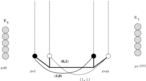
Figure 3: Type IIB gauge bosons enhancing $E_{8}\times E_{8}\times U(1)^{2}\rightarrow E_{8}\times E_{8}\times SU(3)$. Each blob represents one dynamical unit, ${\bf AC}$.

In the equivalent Type IIB picture we want to compute explicitly the mass for a $(p,q)$-string stretching between the two points of $U(1)$ gauge symmetry, ie, $1$ and $z_{s}$ (see Fig 2). First a simple analysis of the moduli tells us that there are 6 strings that can end on the non-local branes sitting at that points. In our conventions these strings are, up to global $SL(2,Z)$ monodromies, ${\bf V^{1,2}}=\pm(1,0),{\bf V^{3,4}}=\pm(1,1)\,\,\&\,\,{\bf V^{5,6}}=\pm(0,1)$. This fixes the tension in the mass formula. The integral in the numerator of the mass formula can be rewritten in terms of hypergeometric functions after a simple change of variables. We obtain

$${\cal L}=\int_{1}^{z_{s}}|\Delta^{-\frac{1}{12}}|=\frac{\sqrt{\pi}(-1)^{5/6}(1-z_{s})^{2/3}\Gamma[5/6]F_{2,1}[5/6,5/6,5/3,1-z_{s}]}{2^{2/3}\Gamma[4/3]}.$$ (4.8)

The periods of $K3$, using eq(3.6), are also expressible in terms of hypergeometric functions. In fact,

$$w_{0} = -2(-1)^{2/3}\pi{\bf F}_{2,1}[1/6,1/6,1,z_{s}])A(e^{i\pi/3})$$ (4.9)

$$w_{1} = 2(-1)^{5/6}\pi(-z_{s})^{-1/6}F_{2,1}[1/6,1/6,1,\frac{1}{z_{s}}]A(e^{i\pi/3}).$$ (4.10)

Through a non-trivial hypergeometric transformation we can rewrite ${\cal L}$ in terms of the periods $w_{i}$ as follows

$${\cal L} = -\frac{\sqrt{\pi}}{2^{5/3}}\frac{\Gamma[5/3]\Gamma[1/6]}{\Gamma[4/3]}(e^{-2\pi i/3}w_{0}+w_{1})$$ (4.11)

$$= -e^{i\pi/3}w_{0}+w_{1}$$

Following [16] we divide the original expression for the mass, eq(3.3), by the fundamental period $w_{0}$ and use the flat coordinate for $K3$, $T_{{\tiny IIB}}=w_{1}/w_{0}$. The result is

$$M_{IIB}(p,q) = \biggl{|}\frac{\eta(e^{i\pi/3})^{2}}{A(e^{i\pi/3})}\biggr{|}|(p+\tau q)(e^{i\pi/3}-T_{{\tiny IIB}})|$$ (4.12)

$$= \biggl{|}\frac{\eta(e^{i\pi/3})^{2}}{A(e^{i\pi/3})}\biggr{|}|(p+\tau q)(\tau-T_{{\tiny IIB}})|$$

Using the $(p,q)$ charges of the strings in Fig. 2 we find complete agreement among the BPS gauge fields responsible for the enhancement of $E_{8}\times E_{8}\times U(1)_{G}^{2}\rightarrow E_{8}\times E_{8}\times SU(3)_{G}$ in the Heterotic string and Type IIB by mapping

$$U_{h} \rightarrow \tau$$ (4.13)

$$T^{0}_{h} \rightarrow T_{{\tiny IIB}}$$ (4.14)

The overall constants are absorbed in the relation between the metrics of the two theories.

We now consider the case with Wilson lines turned on.

b) An example with non-zero Wilson line:
${\bf E_{8}\times E_{8}\times SU(3)_{G}\rightarrow E_{8}\times U(1)^{2}_{G}\times G_{1}\times G_{2}}$

In Fig 3 we represent the configuration we will consider in this subsection from the Type IIB perspective. We break one of the $E_{8}$’s by moving away an integer number of dynamical units. It is not necessary to specify in detail what the breaking is at infinity. The elliptic $K3$ surface equivalent to this configuration in Type IIB is given by

$${\bf K3}\;\;\;\;\;y^{2}+x^{3}+z^{5}(z-1)(z-z_{s})(z-M)^{n}=0.$$ (4.15)

We have put five dynamical units at $z=0$ forming a $E_{8}$, one dynamical units at $z=z_{s}$ and another one at $z=1$ forming $U(1)_{G}^{2}$. At $M$ we have a block formed by $n\leq 5$ dynamical units that have moved away from infinity.

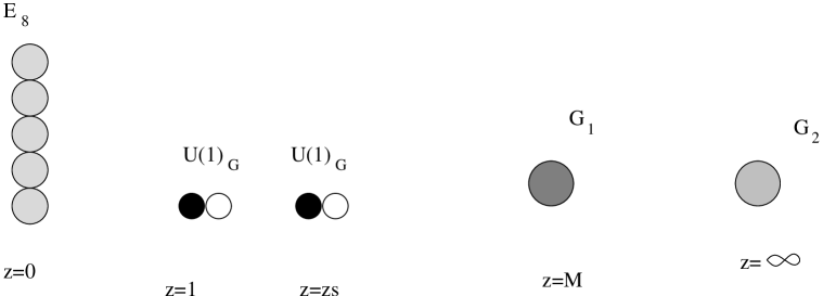
Figure 4: Symmetry breaking. $E_{8}\times E_{8}\times SU(3)_{G}\rightarrow E_{8}\times U(1)^{2}_{G}\times G_{1}\times G_{2}$. Where $G_{1}$ and $G_{2}$ are the gauge groups left unbroken when $n$ dynamical units move away from $z=\infty$.

As before we want to compute

$${\cal L}=\int_{z_{s}}^{1}\Delta^{-\frac{1}{12}}=\int_{z_{s}}^{1}z^{-\frac{5}{6}}(z-1)^{-\frac{1}{6}}(z-z_{s})^{-\frac{1}{6}}(z-M)^{-\frac{n}{6}}.$$ (4.16)

For the periods we have similarly

$$w_{0} = \int_{0}^{z_{s}}z^{-\frac{5}{6}}(z-1)^{-\frac{1}{6}}(z-z_{s})^{-\frac{1}{6}}(z-M)^{-\frac{n}{6}}$$ (4.17)

$$w_{1} = \int_{0}^{1}z^{-\frac{5}{6}}(z-1)^{-\frac{1}{6}}(z-z_{s})^{-\frac{1}{6}}(z-M)^{-\frac{n}{6}}$$ (4.18)

To write ${\cal L}$ in terms of the periods as we did before it turns out to be convenient this time to Taylor expand ${\cal L}$ and the periods in a series in $z/M$. We can now write

$${\cal L}=\sum_{l=0}^{\infty}C_{l}(n)\int_{z_{s}}^{1}z^{l-\frac{5}{6}}(z-1)^{-\frac{1}{6}}(z-z_{s})^{-\frac{1}{6}}.$$ (4.19)

where $C_{l}(n)$ are some numerical coefficients. We also obtain similar expressions for the periods. The point is that we can now rewrite the integrand in terms of hypergeometric functions and apply one of Kummer’s relations to each element in the sum separately as we show in appendix A. It turns out that we end up with the following relation among ${\cal L}$ and the periods

$${\cal L}=w_{0}\tau-w_{1}.$$ (4.20)

Dividing by $w_{0}$ we obtain for the mass formula of BPS states stretching between the 7 branes sitting at $z=1$ and those at $z=z_{s}$

$$M_{IIB}=\biggl{|}\frac{\eta(e^{\frac{i\pi}{3}})^{2}}{A(e^{\frac{i\pi}{3}})}\biggr{|}|(p+\tau q)(\tau-T_{{\tiny IIB}})|.\\$$ (4.21)

where we introduced once again $T_{{\tiny IIB}}$. Note that $T_{{\tiny IIB}}$ incorporates all the information on the positions of the branes as we move them around very much as $T_{h}$ does with Wilson lines. We start now to explore how they are connected.

Heterotic String Duals

Consider a smooth modification of the background of the Heterotic string considered before by turning on Wilson line moduli. The moduli now becomes

$$T = (\frac{B}{2}+\frac{{\bf A_{9}\cdot A_{9}}}{2}\frac{g_{12}}{g_{22}}-\frac{{\bf A_{9}\cdot A_{8}}}{2})+i\frac{\sqrt{g}}{2}(1+\frac{{\bf A_{9}\cdot A_{9}}}{g_{22}})$$ (4.22)

$$= T^{0}+(\frac{{\bf A_{9}\cdot A_{9}}}{2}\frac{g_{12}}{g_{22}}-\frac{{\bf A_{9}\cdot A_{8}}}{2})+i(\frac{\sqrt{g}}{2}\frac{{\bf A_{9}\cdot A_{9}}}{g_{22}}).$$

Let us assume further that the geometrical moduli remain fixed to their values as in eq(4.5). The BPS mass for the $SU(3)_{G}$ states is now given by

$$M_{h}=\frac{1}{2T^{0}_{2}U_{2}}|m_{8}-Um_{9}+Tw^{9}+(TU+Z)w^{8}|$$ (4.23)

Let us analyse what are the conditions for the $SU(3)_{G}$ gauge bosons to become massless again. We surely expect this to be smoothly related to the Wilson lines parameters. In fact, we have

i) For ${\bf V^{1,2}}$:

$$w^{8}=0,\;\;m_{8}=0,\;\;m_{9}=w^{9}.$$ (4.24)

We have for the mass of this states

$$M_{h}=\frac{1}{2T^{0}_{2}U_{2}}|m_{9}(U-T)|.$$ (4.25)

Level matching condition, eq(2.7), implies that $m_{9}w^{9}=1$, ie $w^{9}=\pm 1=m_{9}$, and this will determine, as before, the $p$ charge of the $(p,q)$-string in Type IIB. Note that $T$ depends on the Wilson line parameter now. So to obtain a massless state we must have, $T\rightarrow U$, or from eq(4.22)

$${\bf A_{9}}\cdot{\bf A_{9}} = 0\rightarrow{\bf A_{9}}={\bf 0}$$

$${\bf A_{9}}\cdot{\bf A_{8}} = 0.$$ (4.26)

${\bf ii)}$ For ${\bf V^{3,4}}$

$$m_{8}=w^{8}=-w^{9},\;\;\;m_{9}=0$$ (4.27)

we obtain for the mass

$$M_{h} = \frac{1}{2T^{0}_{2}U_{2}}|w^{8}(1+T-TU-Z)|$$ (4.28)

$$\overrightarrow{=}^{T=U} \frac{1}{2T^{0}_{2}U_{2}}|w^{8}(1+U-U^{2}-Z)|$$

$$\overrightarrow{=}^{U^{2}-U+1=0} \frac{1}{2T^{0}_{2}U_{2}}|w^{8}||Z|\;\;\;\longrightarrow Z=0.$$

Note again that level matching requires $w^{8}=\pm 1=m_{8}\rightarrow w^{9}=\mp 1$. Let’s analyse the condition on $Z$. Using $U=e^{\frac{i\pi}{3}}$ in eq(2.11) we obtain

$$Z=\frac{1}{4}({\bf A_{9}\cdot A_{9}}+2{\bf A_{9}\cdot A_{8}}-2{\bf A_{8}\cdot A_{8}})+i\frac{\sqrt{3}}{2}({\bf A_{9}\cdot A_{8}}-\frac{{\bf A_{9}\cdot A_{9}}}{2})=0.$$ (4.29)

The imaginary part is equal to zero due to eq(4.26). For the real part we have

$${\bf A_{8}\cdot A_{8}}=0\rightarrow{\bf A_{8}}={\bf 0}.$$ (4.30)

These states become massless only when we turn off the Wilson lines, ${\bf A_{i}}={\bf 0}$, as expected. Since in this case we are back to the situation of [16] with the geometrical parameters fixed to their critical values. And Finally

${\bf iii)}$ For ${\bf V^{5,6}}$:

$$w^{9}=0,\;\;w^{8}=m_{8}=m_{9}$$ (4.31)

Level matching requires $w^{8}=\pm 1=m_{8}=m_{9}$. Their mass is given by

$$M_{h} \overrightarrow{=}^{T=U} \frac{1}{2T^{0}_{2}U_{2}}|w_{8}(1-U+TU-Z)|$$ (4.32)

$$= \frac{1}{2T^{0}_{2}U_{2}}|w_{8}||Z|=0.$$

So for the geometrical parameters fixed to their critical values, $B=1$, $R_{c}^{2}=g_{22}=g_{11}=2$ and $g_{12}=1$, we see, by comparing eq(4.22) with eq(4.26), eq(4.29) and eq(4.33), that the relative separation parameter of the two dynamical units on Type IIB responsible for the geometrical enhancement is mapped to the Wilson line moduli by

$$U_{h} \rightarrow \tau$$

$$T_{h} \rightarrow T_{IIB}.$$ (4.33)

If we now consider the more general case when we allow for the geometrical parameters to be different from their critical values the six gauge bosons will become massless again when

$$e^{\frac{i\pi}{3}}=U = T$$

$$\frac{1}{2}+i\frac{\sqrt{3}}{2}=\frac{g_{12}}{g_{22}}+i\frac{\sqrt{g}}{g_{22}} = (\frac{B}{2}+\frac{{\bf A_{9}\cdot A_{9}}}{2}\frac{g_{12}}{g_{22}}-\frac{{\bf A_{9}\cdot A_{8}}}{2})+i\frac{\sqrt{g}}{2}(1+\frac{{\bf A_{9}\cdot A_{9}}}{g_{22}})$$ (4.34)

If we were to turn on a Wilson line and still keep the $SU(3)_{G}$ symmetry we would have to tune the geometrical parameters such that the critical values would be shifted as follows

$$B = 1+{\bf A_{9}\cdot A_{8}}-\frac{{\bf A_{9}\cdot A_{9}}}{2}$$ (4.35)

$$R_{c}^{2} = 2-\frac{{\bf A_{9}\cdot A_{9}}}{2}.$$ (4.36)

Note that the constraints in $Z$, eq(4.28), would still be in place but now in the more general form

$${\bf A_{9}\cdot A_{8}} = \frac{{\bf A_{9}\cdot A_{9}}}{2}$$ (4.37)

$${\bf A_{9}\cdot A_{9}} = {\bf A_{8}\cdot A_{8}}.$$

We have shown that by introducing the parameters $U$ and $T$ as in eq(2.10) and by writing the Heterotic mass formula as in eq(2.13) the map between Heterotic string BPS states and their duals in Type IIB theory are immediately obtained, eq(4.33). In the next section we extend this analysis to the other non-trivial branch of constant coupling in Type IIB theory.

4.2 Branch II - ${\bf\tau=i}$

For branch II, $f\neq 0\;\;\&\;\;g=0\rightarrow\tau=i$, and there are 5 complex degrees of freedom. In fact, $f(\xi)$ is a polynomial of degree 8 and we have to mod out the $SL(2,{\bf C})$ symmetry. The 24 branes join up forming 8 groups with two mutually local branes and a non-local one. In our conventions a dynamical unit is (${\bf AAC}$). In general, we have $SU(2)^{8}$ gauge group. The other possible gauge groups are

$$\begin{array}[]{lll}SU(2)^{8}&E_{7}\times SU(2)^{5}&E_{7}\times E_{7}\times SU(2)^{2}\\ SO(8)\times SU(2)^{6}&E_{7}\times SO(8)\times SU(2)^{3}&E_{7}\times E_{7}\times SO(8)\\ SO(8)^{2}\times SU(2)^{4}&E_{7}\times SO(8)^{2}\times SU(2)&\\ SO(8)^{3}\times SU(2)^{2}&&\\ SO(8)^{4}&&\\ \end{array}$$

Therefore, we see that in Branch II we have two basic gauge enhancements depending on how many dynamical units collide at the same point. We have

$$(SU(2)\times U(1))^{2}\rightarrow SO(8);\;\;\;\&\;\;\;(SU(2)\times U(1))^{3}\rightarrow E_{7}\;\;\;;$$

The mass for BPS $(p,q)$-strings in this branch is given by

$$M_{IIB}(p,q)=\biggl{|}\frac{\eta(i)^{2}}{A(i)}\biggr{|}\frac{\int dz|\Delta(z)^{(-1/12)}|}{|\int_{\gamma_{0}}dz\Delta(z)^{(-1/12)}|}$$ (4.44)

Let us consider the map of IIB theory in Branch II to the $Spin(32)/Z_{2}$ Heterotic String on $T^{2}$. It is convenient to start with the following Wilson lines:

$${\bf W_{8}} = (\frac{1}{2}^{4};\frac{1}{2}^{4};0^{2};0^{2};0^{4})$$

$$\bf W_{9} = (0^{4};\frac{1}{2}^{4};0^{2};0^{2};\frac{1}{2}^{4}).$$ (4.45)

These Wilson lines break the gauge group to $SO(8)^{4}$. The semicolon separation will become clear below.

As part of our duality map we set as before

$$U_{h}\rightarrow\tau.$$ (4.46)

In the Heterotic side this implies that

$$U_{h}=\frac{g_{89}}{g_{99}}+i\frac{\sqrt{g}}{g_{99}}=\tau=i.$$ (4.47)

This fixes two of the geometrical moduli, namely, $g_{89}=0$ and $g_{88}=g_{99}=R^{2}$. This is why in our redefinition of the geometrical parameters in Heterotic string with Wilson lines we left $U_{h}$ unchanged so that this mapping remains the same.

We analyse the map between the Heterotic and type IIB theories in two examples. Both examples correspond to a one-parameter family in the respective moduli spaces.

Once we define a one-parameter family in the Heterotic theory we present a one-parameter family in the Type IIB theory that we argue is the dual family. There is, obviously, an infinity number of one-parameter families in a 5 dimensional space as the moduli space we are dealing with here. Nevertheless, we manage to identify one potential family in the Type IIB theory. The condition for this family to be the dual family of the one in the Heterotic theory is that they both have the same pattern of gauge enhancements taking place in dual points in the moduli spaces. And the fact that the mass of BPS gauge bosons are the same every where in moduli space. We verify this to be the case in both examples we consider. We then write explicitly the duality map between the moduli of the two theories.

We start with the enhancement:

a) ${\bf(SU(2)\times U(1))^{2}\times SO(8)^{3}\rightarrow E_{7}^{2}\times SO(8)}$

To achieve this enhancement we have to move in the Wilson lines moduli space by adding to the Wilson lines above the following pieces

$${\bf A_{8}} = {\bf W_{8}}+(0^{4};0^{4};a^{2},0^{2};0^{4})$$

$${\bf A_{9}} = {\bf W_{9}}+(0^{4};0^{4};0^{2},a^{2};0^{4}),$$ (4.48)

where $a$ is a real positive parameter. It is immediate to see that the effect of the perturbation is to break the third $SO(8)_{(3)}$, ie, the one occupying the third block of four slots in the lattice vector above, to $(SU(2)\times U(1))_{(1)}\times(SU(2)\times U(1))_{(2)}$. We anticipate the map with type IIB by picturing this breaking in Fig 4.

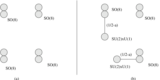
Figure 5: Symmetry breaking in Branch II. Each blob represents one dynamical unit ${\bf AAC}$. a) $SO(8)^{4}$ b)$(SU(2)\times U(1))_{(1)}\times(SU(2)\times U(1))_{(2)}\times SO(8)^{3}$

Note that for $a=\frac{1}{2}$ we have $(SU(2)\times U(1))_{(1)}\rightarrow SO(4)_{(1)}$ and similarly $(SU(2)\times U(1))_{(2)}\rightarrow SO(4)_{(2)}$ since the following vectors become massless (we will concentrate on one of the enhancements to $E_{7}$ only since the process is identical for both)

$${\bf Q}^{(1)}=\pm(0^{4};0^{4};+1,+1;0^{2};0^{4}).$$ (4.49)

We also have states in the vector representation of $SO(4)_{(1)}\times SO(8)_{(1)}$ becoming massless when $a=1/2$

$${\bf Q}^{(2)}=(\underbrace{\pm 1,0^{3}}_{\mbox{p}};0^{4};\underbrace{\pm 1,0}_{\mbox{p}};0^{2};0^{4})=(8_{v};1,4;1;1).$$ (4.50)

These gauge bosons enhance $(SO(4)_{(1)}\times SO(8)_{(1)})\rightarrow SO(12)_{(1)}$. Analogously, we also have $(SO(4)_{(2)}\times SO(8)_{(4)})\rightarrow SO(12)_{(2)}$. The mass of this states as they approach $a=\frac{1}{2}$ are listed in Table 5.

If this model is to represent a configuration of branes in Type IIB in Branch II there can not be a $SO(12)$. But we are not finished yet. We have to check the states with winding numbers.

If we rewrite the expression for the heterotic momenta using $U_{h}=i$ we can write for the mass, eq(2.6),

$$M_{h}^{2}=P_{iR}^{2}=(p_{8}-(g_{88}w^{8}-Bw^{9})\frac{1}{\alpha^{\prime}})^{2}g^{88}+(p_{9}-(g_{99}w^{9}+Bw^{8})\frac{1}{\alpha^{\prime}})^{2}g^{99}$$ (4.51)

and using $g^{88}=g_{99}/g=1/g_{88}=R^{-2}=g^{99}$ we write

$$M_{h}^{2}=P_{iR}^{2}=(p_{8}-(R^{2}w^{8}-Bw^{9})\frac{1}{\alpha^{\prime}})^{2}R^{-2}+(p_{9}-(R^{2}w^{9}+Bw^{8})\frac{1}{\alpha^{\prime}})^{2}R^{-2}$$ (4.52)

For massless states we must have

$$p_{8} = ((R^{2}w^{8}-Bw^{9})\frac{1}{\alpha^{\prime}})$$ (4.53)

$$p_{9} = (R^{2}w^{9}+Bw^{8})\frac{1}{\alpha^{\prime}})$$ (4.54)

Substituting this in the formula for level matching condition for gauge bosons, $P_{L}^{2}=4/\alpha^{\prime}$, we obtain

$$R^{2}((w^{8})^{2}+(w^{9})^{2})=\alpha^{\prime}(1-\frac{q^{2}}{2})$$ (4.55)

This equation requires that we have $q^{2}\leq 2$. Defining $\Lambda=q+\lambda$, $\lambda\in\Gamma^{16}$ such that $\Lambda^{2}$ is smallest. We obtain

$$R^{2}((w^{8})^{2}+(w^{9})^{2})=\alpha^{\prime}(1-\frac{\Lambda^{2}}{2})$$ (4.56)

We separate the winding states in odd and even values for the sake of the analysis. Furthermore, it is easy to see that for odd winding numbers only $w^{i}=\pm 1$ contribute with massless states. For $w^{9}=\pm 1$ and $w^{8}=0$ we obtain ${\bf q}={\bf Q}\pm(0^{4};\frac{1}{2}^{4};0^{2};(\frac{1}{2})^{6})$. Choosing

$${\bf Q}=\mp(\underbrace{\underbrace{(\pm\frac{1}{2})^{4}};(\frac{1}{2})^{4};\underbrace{(\pm\frac{1}{2})^{2}}}_{\mbox{(e\# -)}};(\frac{1}{2})^{2};(\frac{1}{2})^{4})$$ (4.57)

we obtain

$$\Lambda=(\underbrace{(\pm\frac{1}{2})^{4};0^{4};(\pm\frac{1}{2})^{2}}_{\mbox{(e\# -)}};0^{2};0^{4}),$$ (4.58)

These are the spinors ${\bf 32}_{\pm 1}$ of $SO(12)_{(1)}$. The subscript is the $U(1)_{w^{9}}$ charge associated to winding along $x^{9}$-direction. This gauge vectors become massless at the critical radius $R_{c}^{2}=\frac{\alpha^{\prime}}{4}$. It turns out that it is convenient to write the spinors in terms of the gauge groups $SO(8)_{(1)}\times(SU(2)\times U(1))_{(1)}$, ie, ${\bf 32}_{\pm 1}=({\bf 8_{s}};{\bf 1};{\bf 1};{\bf 1};{\bf 1})_{\pm\frac{1}{2}}+({\bf 8_{c}};{\bf 1};{\bf 2};{\bf 1};{\bf 1})$. For even winding numbers, only $w^{i}=\pm 2$ contribute. In this case we take ${\bf Q}=\pm(0^{4};(1)^{4};0^{2};(1)^{6})$ and $\Lambda^{2}=0$, these are singlets, $({\bf 1,1,1,1,1})_{\pm 2}$. These singlets become massless at the same radius as the spinors. So for $R_{c}^{2}=\frac{\alpha^{\prime}}{4}$ the spinors and singlets enhance $SO(12)_{(1)}\times U(1)_{w^{9}}$ to $E_{7}^{(1)}$. Analogously, gauge fields with quantum numbers $w^{9}=0$ and $w^{8}=\pm 1,\pm 2$ enhance $SO(12)_{(2)}\times U(1)_{w^{8}}$ to $E_{7}^{(2)}$.

Note that from eq(4.53) when $w^{8}=0$ and $w^{9}=\pm 1,\pm 2$, as above, we have a constraint in the value of the anti-symmetric field $B$. A straight forward analysis of that equation shows that we must have $B\in 2Z$ (this only fixes $B$ up to an $SL(2,Z)$ transformation). Therefore, we choose $B=0$. This fixes the real part in the mass formula, eq(2.13), as in Table 5.

Consider now the other two free moduli. We have the Wilson line parameter, $a$, and the radius, $R^{2}=g_{88}=g_{99}$. As mentioned before, we will consider only one-parameter families. So we have to fix one of this parameters. We know that when we are at the critical radius as $a\rightarrow 1/2$ we obtain the enhancements described above. Therefore, we choose the radius to be a function of $a$ so that at $a=1/2$ we have $R^{2}=R_{c}^{2}=\alpha^{\prime}/4$. Of course there are an infinity number of ways of achieving this but ultimately we want a match between the masses of BPS states in the dual theories. The analysis carried out in Appendix B determines that we set for the specific choice of parameters in the Type IIB side to discussed below

$$R^{2}=\alpha^{\prime}\bigl{(}a(1-a)-(\frac{1}{2}-a)\bigr{)}.$$ (4.59)

It is now possible to write the mass formula for all the BPS states we have been considering in this section. We write their mass in terms of the mass formula, eq(2.13). The results are summarised in Table 5.

${\bf Q}$	$M_{h}$
$(\pm(0^{4};0^{4};+1,+1;0^{2};0^{4})$	$\frac{4}{\alpha^{\prime}}|2(\frac{1}{2}-a)|$
$({\bf 8_{v}};{\bf 1};{\bf 2};{\bf 1};{\bf 1})_{0}$	$\frac{4}{\alpha^{\prime}}|(\frac{1}{2}-a)|$
$({\bf 8_{v}};{\bf 1};{\bf 1};{\bf 1};{\bf 1})_{\pm 1}$	$\frac{4}{\alpha^{\prime}}|(\frac{1}{2}-a)|$
$({\bf 8_{c}};{\bf 1};{\bf 2};{\bf 1};{\bf 1})_{0}$	$\frac{4}{\alpha^{\prime}}|i(\frac{1}{2}-a)|$
$({\bf 8_{s}};{\bf 1};{\bf 1};{\bf 1};{\bf 1})_{\pm\frac{1}{2}}$	$\frac{4}{\alpha^{\prime}}|(-1+i)(\frac{1}{2}-a)|$
$({\bf 1};{\bf 1};{\bf 1};{\bf 1};{\bf 1})_{\pm 2}$	$\frac{4}{\alpha^{\prime}}|(2i(\frac{1}{2}-a)|$

Table 5: Additional gauge bosons for $SO(8)_{(1)}\times(SU(2)\times U(1))_{(1)}\times U(1)_{w^{9}}\rightarrow E_{7}^{(1)}$

Type IIB duals

In type IIB theory starting from an $SO(8)^{4}$ configuration we move the two dynamical units forming one of the $SO(8)$s in perpendicular directions toward two $SO(8)$s (see Fig. 4). As each of the dynamical units approach one of the $SO(8)$s a number of $(p,q)$-strings will become massless. We identify this strings by their symmetry properties and compute their mass near the point they become massless.

For the $SU(2)\times U(1)$ in Type IIB we have ${\bf AAC}={\bf BAA}$. The two vectors in the adjoint of $SU(2)$ correspond to the ${\bf A}\rightarrow{\bf A}$ $(1,0)$-string with both orientations. The enhancement to $SO(4)$ occurs when strings (prongs) like the ones in Fig. 6 become massless. They are equivalent to the vectors ${\bf Q}^{(1)}=\pm(0^{4};0^{4};+1,+1;0^{2};0^{4})$. The $\pm$ correspond to orientation.

Figure 6: For ${\bf Q^{(1)}}=\pm(0^{4};0^{4};1,1;0^{2};0^{4})$. In b) we show the string junction equivalent to the string going across branch cuts in a). They are connected through a string creation process.

For the states in the vector representation, ${\bf Q}^{(2)}=({\bf 8_{v}},{\bf 1},{\bf 4};{\bf 1};{\bf 1})$, of $SO(8)_{(1)}\times SO(4)_{(1)}$ we separate it in two parts in terms of $SO(8)_{(1)}\times(SU(2)\times U(1)^{2})_{(1)}$. One where the permutations have the same signs, ${\bf Q}_{a}^{(2)}=(\pm\underbrace{+1;0^{3}}_{\mbox{p}};0^{4};\underbrace{+1,0}_{\mbox{p}};0^{2};0^{4})$ and the other where the permutations have opposite signs, ${\bf Q}_{b}^{(2)}=\pm(\underbrace{-1;0^{3}}_{\mbox{p}};0^{4};\underbrace{+1,0}_{\mbox{p}};0^{2};0^{4})$. We identify ${\bf Q}_{a}^{(2)}$ with the strings (prongs) in Fig 6 and ${\bf Q}_{b}^{(2)}$ with Fig 7.

Figure 7: ${\bf Q}_{a}^{(2)}$

Figure 8: For ${\bf Q}_{b}^{(2)}$. Two equivalent configurations are shown.

For the spinors we identify ${\bf q}_{a}=({\bf 8_{c}};{\bf 1};{\bf 2};{\bf 1};{\bf 1})$ with the configurations exemplified in Fig 8. And ${\bf q}_{b}=({\bf 8_{c}};{\bf 1};{\bf 2};{\bf 1};{\bf 1})$ is identified with Fig 9.

Figure 9: For ${\bf q}_{a}=({\bf 8_{c}};{\bf 1};{\bf 2};{\bf 1};{\bf 1})$. Two equivalent representations of this BPS state are shown in a) and b).

Figure 10: For ${\bf q}_{b}=({\bf 8_{c}};{\bf 1};{\bf 2};{\bf 1};{\bf 1})$. The O7-plane (CB) branch cut has been shifted to the right to simplify the drawing. Once again two equivalent configurations are shown.

We now compute the mass for each of this configurations. The $K3$ surface equivalent to the configuration of branes in Fig. 4 is given by

$${\bf K3}\;\;\;:\;\;\;y^{2}+x^{3}+x(z^{2}(z-1)^{2}(z-z_{s}))$$ (4.60)

We obtain for the integral of the discriminant of this $K3$

$${\cal L}=\int_{1}^{z_{s}}\Delta^{-\frac{1}{12}}=i\sqrt{\pi}(1-z_{s})^{\frac{1}{4}}\frac{\Gamma[\frac{3}{4}]}{\Gamma[\frac{5}{4}]}F_{1}(\frac{1}{2},\frac{1}{2},\frac{5}{4},1-z_{s})$$ (4.61)

For the periods we obtain

$$w_{0} = -(-1)^{\frac{1}{4}}\sqrt{\pi}(z_{s})^{\frac{1}{4}}\frac{\Gamma[\frac{3}{4}]}{\Gamma[\frac{5}{4}]}F_{1}(\frac{1}{2},\frac{1}{2},\frac{5}{4},z_{s})$$ (4.62)

$$w_{1} = -i(-1)^{\frac{1}{4}}\pi(z_{s})^{-\frac{1}{4}}F_{1}(\frac{1}{4},\frac{1}{2},1,\frac{1}{z_{s}}).$$ (4.63)

By means of a non-trivial Hypergeometric transformation we can write

$${\cal L}=w_{0}+iw_{1}$$ (4.64)

And we obtain for the mass of a $(p,q)$-string

$$M_{IIB}(p,q)=\biggl{|}\frac{\eta(i)^{2}}{A(i)}\biggr{|}|(p+iq)(i)(i-T_{{\tiny IIB}})|$$ (4.65)

We can now compare the masses of BPS gauge fields in both theories. The results are summarised in Table 6. It is clear that the explicit duality map is given by

$$U_{h} \rightarrow \tau$$

$$|(\frac{1}{2}-a)| \rightarrow |i(i-T_{{\tiny IIB}})|.$$ (4.66)

${\bf V}$	$\frac{\alpha^{\prime}}{4}M_{h}$	$(\frac{A(i)}{\eta(i)^{2}})M_{IIB}$
$(\pm(0^{4};0^{4};+1,+1;0^{2};0^{4})$	$|(2)(\frac{1}{2}-a)|$	$|(2)[i(i-T_{{\tiny IIB}})]|$
$({\bf 8_{v}};{\bf 1};{\bf 2};{\bf 1};{\bf 1})_{0}$	$|(\frac{1}{2}-a)|$	$|[i(i-T_{{\tiny IIB}})]|$
$({\bf 8_{c}};{\bf 1};{\bf 2};{\bf 1};{\bf 1})_{0}$	$|(i)(\frac{1}{2}-a)|$	$|(i)[i(i-T_{{\tiny IIB}})]|$
$({\bf 8_{s}};{\bf 1};{\bf 1};{\bf 1};{\bf 1})_{\pm\frac{1}{2}}$	$|(-1+i)(\frac{1}{2}-a)|$	$|(-1+i)[i(i-T_{{\tiny IIB}})]|$
$({\bf 1};{\bf 1};{\bf 1};{\bf 1};{\bf 1})_{\pm 2}$	$|(2i)(\frac{1}{2}-a)|$	$|(2i)[i(i-T_{{\tiny IIB}})]|$

Table 6: Heterotic-IIB map for the gauge bosons of $SO(8)_{(1)}\times(SU(2)\times U(1))_{(1)}\times U(1)_{w^{9}}\rightarrow E_{7}^{(1)}$.

In the next sub-section we consider the vector bosons responsible for the enhancement of $SU(2)\times U(1)\rightarrow SO(8)$.

b) ${\bf SO(8)\rightarrow SU(2)\times U(1)}$

In the previous section we identified the $(p,q)$-strings configurations that are responsible for the enhancement to $E_{7}$. To complete the symmetry enhancements possible in the this branch we here consider the enhancement $(SU(2)\times U(1))^{2}\rightarrow SO(8)$. We choose, for convenience, to do this through $E_{7}^{2}\times(SU(2)\times U(1))\times(SU(2)\times U(1))\rightarrow E_{7}^{2}\times SO(8)$ (see Fig. 10). We choose to put one of the $E_{7}$’s at $z=\infty$ and the other one at $z=0$. We also put one of the $SU(2)\times U(1)$ at $z=1$ and the other at $z=z_{s}$.

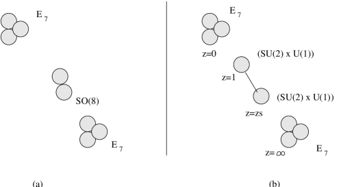
Figure 11: $E_{7}^{2}\times(SU(2)\times U(1))\times(SU(2)\times U(1))\rightarrow E_{7}^{2}\times SO(8)$

The mass of a $(p,q)$-string stretching from one dynamical unit (${\bf AAC}$) to the other is of the form

$$M(p,q)=\biggl{|}\frac{\eta(i)^{2}}{A(i)}\biggr{|}|(p+iq)\frac{{\cal L}}{w_{0}}|$$ (4.67)

With the configuration above we obtain for the integral of the discriminant

$${\cal L}=\frac{2}{\sqrt{\pi}}e^{3\pi i/4}(1-z_{s})^{1/2}\Gamma[3/4]^{2}F{1,2}(3/4,3/4,3/2,1-z_{s})$$ (4.68)

For the $K3$ periods we obtain

$$w_{0} = e^{i\pi/2}\sqrt{2}\pi F_{1,2}(1/4,1/4,1,z_{s}).$$ (4.69)

$$w_{1} = e^{-i\pi/4}\sqrt{2}\pi(-z_{s}^{-1/4})F_{1,2}(1/4,1/4,1,1/z_{s}).$$ (4.70)

We now use one of Kummer’s relations for Hypergeommetric functions to write

$$\frac{\sqrt{\pi}}{2\Gamma[3/2]\Gamma[3/4]}{\cal L}=\frac{\Gamma[1/4]}{\sqrt{2}\pi}e^{i\pi/2}w_{0}-\frac{\Gamma[1/4]}{\sqrt{2}\pi}w_{1}.$$ (4.71)

Therefore we have for the mass of BPS $(p,q)$-strings in this background

$$M_{BPS}^{IIB}(p,q)=\biggl{|}\frac{\eta(i)}{A(i)}\biggr{|}|(p+iq)(i-T_{{\tiny IIB}})|.$$ (4.72)

In the heterotic side we have the vectors below becoming massless to form the ${\bf Adj}$ of $SO(8)$. In the respective figures we draw the $(p,q)$-strings we identify as the dual pairs in the IIB side.

$${\bf Q}^{(1)} = \pm(0^{4},+1,+1,0^{2};0^{8})\;\;\mbox{or}\;\;\pm(0^{4};0^{2};+1,+1;0^{8})\rightarrow\mbox{Fig. 12}$$ (4.73)

$${\bf Q}^{(2)} = \pm(0^{4};-1,0;+1,0;0^{8})\rightarrow\mbox{Fig. 13}$$ (4.74)

$${\bf Q}^{(3)} = \pm(0^{4};+1,0;+1,0;0^{8})\rightarrow\mbox{Fig. 14}$$ (4.75)

In Table 7 we list the masses and quantum numbers of this gauge fields in both theories. The duality map for the moduli space is given by

$$U_{h} \rightarrow \tau$$

$$|(1+i)(\frac{1}{2}-a)| \rightarrow |i-T_{{\tiny IIB}}|.$$ (4.76)

$Q$	$m$	$\frac{\alpha^{\prime}}{4}M_{h}$	$p$	$q$	$\frac{A(i)}{\eta(i)^{2}}M_{IIB}$
$\pm(0^{4},+1,+1,0^{2};0^{8})$	$\pm 1$	$|(1-i)[(1+i)(\frac{1}{2}-a)]|$	$-1$	$1$	$|(1-i)(i-T_{{\tiny IIB}})|$
$\pm(0^{4},0^{2},+1,+1;0^{8})$	$\pm 1$	$|(1-i)[(1+i)(\frac{1}{2}-a)]|$	$-1$	$1$	$|(1-i)(i-T_{{\tiny IIB}})|$
$\pm(0^{4},+1,0,+1,0;0^{8})$	$\mp 1$	$|(i)[(1+i)(\frac{1}{2}-a)]|$	$0$	$1$	$|(i)(i-T_{{\tiny IIB}})|$
$\pm(0^{4},-1,0,+1,0;0^{8})$	$0$	$|[(1+i)(\frac{1}{2}-a)]|$	$1$	$0$	$|(i-T_{{\tiny IIB}})|$

Table 7: BPS gauge fields enhancing $(SU(2)\times U(1))\times(SU(2)\times U(1))\rightarrow SO(8)$ in the Heterotic and IIB. Also $m_{8}=m_{9}=m$ and $w^{8}=w^{9}=w=0$.

Figure 12: ${\bf Q}^{(1)}$ for $(SU(2)\times U(1))\times(SU(2)\times U(1))\rightarrow SO(8)$. Two equivalent configurations are shown.

Figure 13: ${\bf Q}^{(2)}$ for $(SU(2)\times U(1))\times(SU(2)\times U(1))\rightarrow SO(8)$.

Figure 14: ${\bf Q}^{(3)}$ for $(SU(2)\times U(1))\times(SU(2)\times U(1))\rightarrow SO(8)$.

5 Conclusion

In this paper we have analysed the duality between the Heterotic string in 8 dimensions and Type IIB theory in the base space of an elliptically fibred $K3$. The duality map between the relevant BPS states was given in detail in the branches of moduli space of Type IIB with constant coupling.

In Type IIB the flat coordinate, $T_{IIB}=w_{0}/w_{1}$, defined in terms of the periods of the underlying $K3$ geometry encompasses all the information on the position of the 7-branes in the background when the elliptic fibre has constant complex structure. It is therefore the natural coordinate to be used when analysing the map with Wilson lines on the Heterotic string side. In fact, redefining the Kahler structure of the torus, $T_{h}$, in the Heterotic theory to include information on the Wilson lines. We have found that it becomes the natural coordinate to account for the effects of Wilson lines to the mass of BPS states.

For the the case of the $Spin(32)/Z_{2}$ Heterotic string the masses of BPS states for specific values of the Wilson lines were analysed in detail. In particular, we considered the enhancements: $SO(8)\times SU(2)\times U(1)\times U(1)_{G}\rightarrow E_{7}$ and $(SU(2)\times U(1))^{2}\times SO(8)$. In both cases we identified the dual BPS string junctions responsible for the enhancement on the Type IIB side and computed their masses finding complete agreement between the two sets of states.

It would be interesting to consider the case with non constant coupling in Type IIB. Work in this direction is under way.

Appendix A Generalising The Hypergeometric Relation Among ${\cal L}$, $w_{0}$ and $w_{1}$.

Several times in this paper we had to rewrite the distance ${\cal L}$ in terms of the periods of $K3$. In most cases when we have only four groups of dynamical branes in $S^{2}_{s}$ we can rewrite the integrals in terms of hypergeometric functions. It turns out then that the integrals in this form are related by means of the Kummer’s relations[25]. However, when the blocks break apart and we have more then four points in the sphere we cannot write then as hypergeometric functions anymore. Nevertheless, we show that by Taylor expanding the integrand we can write the integrals as a sum of integrals that in turn can be related to hypergeometric functions. We can then apply Kummer’s relations to each element of the sum in separate and sum up the series again to obtain the relation we look for. This generalises the hypergeometric relations to a more general set of integrals. In this appendix we present the details of this calculations for the configuration considered in Section 4.1.

We start with the length of the string stretched from $z=1$ and $z=z_{s}$

$$\int_{z_{s}}^{1}\Delta^{-\frac{1}{12}}=\int_{z_{s}}^{1}z^{-\frac{5}{6}}(z-1)^{-\frac{1}{6}}(z-z_{s})^{-\frac{1}{6}}(z-M)^{-\frac{n}{6}}.$$ (A.1)

we now Taylor expand $(z-M)^{-\frac{n}{6}}$ as

$$(z-M)^{-\frac{n}{6}}=\sum_{l=0}^{\infty}C_{l}(n)z^{l}$$ (A.2)

where $C_{l}(n)$ are standard numerical coefficients. If we now plug this back in eq(A.1) we have

$${\cal L}=\sum_{l=0}^{\infty}C_{l}(n)\int_{z_{s}}^{1}z^{l-\frac{5}{6}}(z-1)^{-\frac{1}{6}}(z-z_{s})^{-\frac{1}{6}}.$$ (A.3)

This integral can be written in terms of hypergeometric functions by doing a simple change of variables, ie, $z\rightarrow(z-z_{s})/(1-z_{s})$. We obtain

$${\cal L}=\sum_{l=0}^{\infty}C_{l}(n)\biggl{(}\frac{\sqrt{\pi}(-1)^{5/6}}{2^{2/3}}\frac{\Gamma[\frac{5}{6}]}{\Gamma[\frac{4}{3}]}F_{2,1}[\frac{5}{6},(\frac{5}{6}-l),\frac{5}{3},1-z_{s}]\biggr{)}.$$ (A.4)

Similarly, we obtain for the periods, eq(4.17) and eq(4.18),

$$w_{0} = \sum_{l=0}^{\infty}C_{l}(n)\biggl{(}\frac{(1-i\sqrt{3})}{2}\frac{\Gamma[\frac{5}{6}]\Gamma[\frac{1}{6}+l]}{\Gamma[1+l]}z_{s}F_{2,1}[\frac{1}{6},(\frac{1}{6}+l),(1+l),z_{s}]\biggr{)}$$ (A.5)

$$w_{1} = -\sum_{l=0}^{\infty}C_{l}(n)\biggl{(}(-1)^{5/6}\frac{\Gamma[\frac{5}{6}]\Gamma[\frac{1}{6}+l]}{\Gamma[1+l]}(-z_{s})^{-\frac{1}{6}}F_{2,1}[\frac{1}{6},(\frac{1}{6}+l),(1+l),\frac{1}{z_{s}}]\biggr{)}.$$ (A.6)

Using the following Kummer relation[25]

$$e^{i\pi 5/6}\frac{\Gamma[\frac{5}{6}]\Gamma[\frac{5}{6}]}{\Gamma[\frac{5}{3}]}(1-z_{s})^{2/3}F_{2,1}[\frac{5}{6},\frac{5}{6}-l,\frac{5}{3},1-z_{s}] = \frac{\Gamma[\frac{5}{6}]\Gamma[\frac{1}{6}+l]}{\Gamma[1+l]}z_{s}F_{2,1}[\frac{1}{6},\frac{1}{6}+l,1+l,z_{s}]+$$

$$= e^{i\pi 5/6}\frac{\Gamma[\frac{5}{6}]\Gamma[\frac{1}{6}+l]}{\Gamma[1+l]}(-z_{s})^{-\frac{1}{6}}F_{2,1}[\frac{1}{6},\frac{1}{6}+l,1+l,\frac{1}{z_{s}}].$$

we can write each element in the series representation of ${\cal L}$ in terms of the respective elements in the series representation of $w_{0}$ and $w_{1}$. Plugging this result back in the sum, eq(A.4), and reexpressing the sum in its closed form, we arrive at the desired relation among ${\cal L}$ and $w_{0}$ and $w_{1}$, ie,

$${\cal L}=\tau w_{0}-w_{1}.$$ (A.7)

It is clear that this procedure can be applied to any distribution of the dynamical units on the sphere by Taylor expanding an appropriate number of terms in the expression for ${\cal L}$, $w_{0}$ and $w_{1}$.

Appendix B Fixing Moduli in Branch II

In Section 4.2 the first example of gauge enhancement in Branch II to be analysed was $SO(8)^{3}\times(SU(2)\times U(1))^{2}\rightarrow E_{7}^{2}\times SO(8)$. To obtain this enhancement the following Wilson lines were turned on

$$A_{8} = (\frac{1}{2}^{4},\frac{1}{2}^{4},a,a,0^{2},0^{4})$$ (B.1)

$$A_{9} = (0^{4},\frac{1}{2}^{4},0^{2},a,a,\frac{1}{2}^{4})$$ (B.2)

with $a=0$ and $a=1/2$ being the critical values for the Wilson lines parameter. This was enough to determine the masses of BPS gauge bosons transforming in the vector and adjoint representations of the gauge groups. With this information we fixed part of the map with the BPS states on the Type IIB theory. We saw also that to obtain the full gauge enhancement we needed BPS states transforming in the spinor and singlet representations of the gauge groups. However, for these states to become massless we need to tune not only the parameter in the Wilson lines but the geometric moduli as well. We want to determine the value of the geometric moduli, $R$ and $B$, such that the masses of the BPS states responsible for the enhancement above match with those in Type IIB. We will concentrate in three specific examples of gauge fields here. The quantum numbers of these states will be given explicitly. The results easily generalise to all other states.

We will concentrate on the spinor with quantum numbers $w^{9}=+1$ and $w^{8}=0$. And the singlet with quantum numbers, $w^{9}=+2$ and $w^{8}=0$. The other quantum numbers will be determined below.

Recall that the critical radius was, eq(4.53), determined in terms of

$$\Lambda=(\pm\frac{1}{2}^{4},0^{4},\pm\frac{1}{2}^{2},a-\frac{1}{2},a-\frac{1}{2},0^{4})$$ (B.3)

as $R_{c}^{2}/2=1-\Lambda^{2}/2=a(1-a)$. Was the radius to be set in this form we would have the spinors and singlets all massless for all values of $a$. However this would generate enhancements that have no equivalent in Branch II on Type IIB. But we know that when $a=1/2$ we must have the appropriate enhancement. One way to guarantee that this is the case is to set $R^{2}/2=1/4$. But it turns out that this choice does not give the right expression for the masses of the spinor and singlets. This means we would be specifying a one-parameter family with the right gauge enhancements but not the dual family of the BPS states we identified on Type IIB. The masses of BPS states on both sides must match as well as the gauge enhancement pattern.

To obtain the correct BPS masses in the Heterotic theory we impose the condition that it matches the ones on Type IIB. This will fix $R$ and $B$.

The analysis naturally separate in two parts. The real part of the mass formula depends on $B$ and $a$ only. The constraint described above will fix $B$ in terms of $a$. The imaginary part depends on the radius, $R$, and $a$ only. The match with the mass formulas on type IIB fixes the relation between the two moduli. The imaginary part is given by

$$Im(M_{h})=m_{9}-A_{9}\cdot Q-w^{9}(\frac{R^{2}}{2}+(1+a^{2})).$$ (B.4)

where we used

$$Im(T) = \frac{\sqrt{g}}{2}+\frac{A_{9}^{2}}{2}$$ (B.5)

$$= \frac{R^{2}}{2}+(1+a^{2}).$$ (B.6)

For the real part we obtain

$$Re(M_{h})=m_{8}-A_{8}\cdot Q+w^{9}(\frac{B}{2}-\frac{1}{2}).$$ (B.7)

where

$$Im(T) = \frac{B}{2}-\frac{A_{8}\cdot A_{9}}{2}$$ (B.8)

$$= \frac{B}{2}-\frac{1}{2}.$$ (B.9)

Now we require that the imaginary part of the masses for both the spinors and singlets to be equal to $(1/2-a)$ in order to agree with the map for the vectors as in Table 6. We choose three specific BPS gauge bosons to carry out the analysis explicitly. The results can be easily extended to all other gauge fields. The representatives we choose are

$$Q^{1} = (0^{4},-1^{4},0^{2},-1^{6})\in({\bf 1,1,1,1,1})$$ (B.10)

$$Q^{2} = (+\frac{1}{2}^{4},-\frac{1}{2}^{4},+\frac{1}{2}^{2},-\frac{1}{2}^{6})\in({\bf 8_{s},1,1,1,1})$$ (B.11)

$$Q^{3} = (+\frac{1}{2},-\frac{1}{2}^{3},-\frac{1}{2}^{4},+\frac{1}{2},-\frac{1}{2},-\frac{1}{2}^{6})\in({\bf 8_{c},1,2,1,1}).$$ (B.12)

First of all we see from eq(B.5) that for this gauge bosons to be massless at $a=1/2$ we must have $m_{9}=-1$ for the spinors and $m_{9}=-2$ for the singlet. Furthermore, requiring agreement with the imaginary part of the masses on the Type IIB theory we obtain

$$\frac{R^{2}}{2}=2a-a^{2}-\frac{1}{2}=\frac{R_{c}^{2}}{2}-(\frac{1}{2}-a).$$ (B.13)

This fixes the radius as a function of the Wilson line parameter.

The requirement that the real part is as in Table 6 yields for $B$

$$Re(M_{h})(Q^{1}) = m_{8}+B\biggl{|}_{a=\frac{1}{2}}=0$$ (B.14)

$$Re(M_{h})(Q^{2}) = (m_{8}-1+\frac{B}{2})\biggl{|}_{a=\frac{1}{2}}=0$$ (B.15)

$$Re(M_{h})(Q^{3}) = (m_{8}+1+\frac{B}{2})\biggl{|}_{a=\frac{1}{2}}=0.$$ (B.16)

These equations imply that $B\in 2Z$. We choose $B=0$ (up to $SL(2,Z)$ transformations). The $m_{8}$ quantum number for the representatives as well as the expression for the real part of the masses away for $a=1/2$ are also fixed. We summarise the results in table 8.

$Q$	$m_{8}$	$m_{9}$	$w^{8}$	$w^{9}$	$Re(M_{h})$	$Im(M_{h})$
$Q^{1}$	$0$	$-2$	$0$	$2$	$0$	$(\frac{1}{2}-a)$
$Q^{2}$	$1$	$-1$	$0$	$1$	$-(\frac{1}{2}-a)$	$(\frac{1}{2}-a)$
$Q^{3}$	$-1$	$-1$	$0$	$1$	$0$	$(\frac{1}{2}-a)$

Table 8: The quantum numbers and masses of the singlet and spinor representatives.

References

- [1] C. Vafa, Evidence for F-theory, Nucl.Phys. B469 (1996) 403-418, hep-th/9602022;
- [2] M. Bershadsky, K. Intriligator, S. Kachru, D. R. Morrison, V. Sadov, C. Vafa, Geometric Singularities and Enhanced Gauge Symmetries, Nucl.Phys. B481 (1996) 215-252, hep-th/9605200;
- [3] K.S. Narain, M.H. Sarmadi , E. Witten, A Note on the Toroidal Compactification of Heterotic String Theory, Nucl.Phys.B279:369,1987;
- [4] P. Ginsparg, Comment on the Toroidal Compactification of Heterotic Superstrings, Phys.Rev.D35:648,1987;
- [5] P. Aspinwall, Enhanced Gauge Symmetries and K3 Surfaces, Phys. Lett. B357 (1995) 329,hep-th/9507012;
- [6] A. Sen, F-theory and Orientifolds, Nucl.Phys. B475 (1996) 562-578;
- [7] A. Johansen, A comment on BPS states in F-theory in 8 dimensions, Phys.Lett.B395 (1997) 36-41, hep-th/9608186.
- [8] M.R.Gaberdiel, B.Zwiebach, Exceptional groups from open strings, Nucl.Phys.B518 (1998) 151, hep-th/9709013.
- [9] M.R.Gaberdiel, T.Hauer, B.Zwiebach, Open string-string junction transitions, Nucl.Phys.B525 (1998) 117, hep-th/9801205.
- [10] Y.Imamura, Flavour Multiplets, Phys.Rev.D58 (1998) 106005, hep-th/9802189.
- [11] O.DeWolfe and B.Zwiebach, String Junctions for Arbitrary Lie Algebra Representations, Nucl.Phys. B541 (1999) 509-565, hep-th/9804210;
- [12] O. DeWolfe, T. Hauer, A. Iqbal, B. Zwiebach, Uncovering the Symmetries on [p,q] 7-branes: Beyond the Kodaira Classification, hep-th/9812028;
- [13] O. DeWolfe, T. Hauer, A. Iqbal, B. Zwiebach, Uncovering Infinite Symmetries on [p,q] 7-branes: Kac-Moody Algebras and Beyond,hep-th/9812209;
- [14] O. DeWolfe, Affine Lie Algebras, String Junctions and 7-Branes, Nucl.Phys. B550 (1999) 622-637, hep-th/9809026;
- [15] Y. Imamura, String Junctions and Their Duals in Heterotic String Theory, Prog.Theor.Phys. 101 (1999) 1155-1164, hep-th/9901001; D. O’Driscoll, Non-Perturbative Structure in Heterotic Strings from Dual F-Theory Models, Phys.Lett. B454 (1999) 240-246, hep-th/9901028;
- [16] W. Lerche, S. Stieberger, Prepotential, Mirror Map and F-Theory on K3, Adv.Theor.Math.Phys. 2 (1998) 1105-1140, hep-th/9804176;
- [17] G. Lopes Cardoso, G Curio, D Lust, T Mohaupt, On the Duality between the Heterotic String and F-Theory in 8 Dimensions, Phys.Lett. B389 (1996) 479-484, hep-th/9609111;
- [18] A. Dabholkar, J. A. Harvey, Non renormalisation of the Superstring Tension., Phys.Rev.Lett.63:478,1989;
- [19] A. Sen, BPS states in a Three Brane Probe, Phys.Rev. D55 (1997) 2501-2503;
- [20] W. Lerche, S. Stieberger, N. P. Warner, Quartic Gauge Couplings from K3 Geometry, hep-th/9811228;
- [21] W. Lerche, S. Stieberger, On the Anomalous and Global Interactions of Kodaira 7-Planes, hep-th/9903232;
- [22] K. Dasgupta, S. Mukhi, F-Theory at Constant Coupling, Phys.Lett. B385 (1996) 125-131, hep-th/9606044;
- [23] G. Lopes Cardoso, D. Lust, T. Mohaupt, Threshold Corrections and Symmetry Enhancement in String Compactifications, Nucl.Phys. B450 (1995) 115-173, hep-th/9412209;
- [24] O. Bergman, M. R. Gaberdiel, G. Lifschytz, String Creation and Heterotic-Type I’ Duality,Nucl.Phys. B524 (1998) 524-544, hep-th/9711098;
- [25] A. Erdelyi, Higher Transcendental Functions - Bateman Manuscript Project, McGraw-Hill, 1953;