DAMTP–1999–119, hep-th/9909168

On the constraints defining BPS monopoles

We discuss the explicit formulation of the transcendental constraints defining spectral curves of $SU(2)$ BPS monopoles in the twistor approach of Hitchin, following Ercolani and Sinha. We obtain an improved version of the Ercolani–Sinha constraints, and show that the Corrigan–Goddard conditions for constructing monopoles of arbitrary charge can be regarded as a special case of these. As an application, we study the spectral curve of the tetrahedrally symmetric 3-monopole, an example where the Corrigan–Goddard conditions need to be modified. A particular 1-cycle on the spectral curve plays an important rôle in our analysis.

1 Introduction

BPS monopoles for the $SU(2)$ Yang–Mills–Higgs gauge theory have been studied for over twenty years, using a number of different approaches. Twistor methods, relating the solutions of the integrable differential equations of the model to holomorphic vector bundles over a so-called twistor space, were first introduced by Ward, adapting previous work on the self-duality equations for the pure Yang–Mills theory on $\mathbb{R}^{4}$. They enabled solutions of magnetic charge $k>1$ to be constructed for the first time [15]. A twistor approach intrinsic to the geometry of $\mathbb{R}^{3}$ was developed later by Hitchin in [7] and [8]. In his formulation, a monopole is associated to a spectral curve, a compact complex curve in $T^{\prime}\mathbb{CP}^{1}$, the total space of the holomorphic tangent bundle of $\mathbb{CP}^{1}$, satisfying a number of conditions which were stated in [8]. Based on this approach, new solutions have been constructed and new characterisations of monopoles developed; we refer to [14] for a brief overview.

The (reduced) moduli space ${\cal N}_{k}$ of gauge-inequivalent BPS monopoles of a given charge $k$ is a $(4k-1)$-dimensional manifold, which has been described in several ways. If we adopt the twistor formulation in terms of spectral curves, it can be characterised as the space of complex curves in $T^{\prime}\mathbb{CP}^{1}$ satisfying a number of transcendental constraints. For the case where the curve is nonsingular, Ercolani and Sinha attempted to formulate these constraints explicitly in [4]; they followed essentially the method of Hurtubise in [12], who achieved a satisfactory description of ${\cal N}_{2}$. Their approach leads to a method of determining constraints on spectral curves by analysing objects of the function theory obtained on them. These constraints parallel the Corrigan–Goddard conditions [3] for constructing $SU(2)$ monopoles, and we shall clarify how they relate to each other.

This paper is organised as follows. We start by introducing the relevant aspects of the twistor approach for monopoles in section 2, in order to fix the notation. In section 3, we review the method of Ercolani and Sinha, and present a new version (24) of their constraint equations which involves a special 1-cycle $c$ on the spectral curve. The Corrigan–Goddard conditions were originally formulated in terms of integrals around the equator of $\mathbb{CP}^{1}$, but we show in section 4 how to interpret them equivalently as integrals on the spectral curve. Moreover, we establish that the conditions in the two methods agree except for one detail: the Corrigan–Goddard approach enforces $c$ to be of a special sort, namely a combination of lifts of the equator of $\mathbb{CP}^{1}$ to the spectral curve. In section 5, we apply the Ercolani–Sinha method to compute the spectral curve of the tetrahedral 3-monopole discussed in [9]. Thereby, the corresponding 1-cycle $c$ is determined and the result shows that the Corrigan–Goddard assumption about $c$ is too restrictive in general; we also consider the action of the tetrahedral group $\mathfrak{A}_{4}\subset SO(3)$ on the homology of the spectral curve and show that it leaves $c$ invariant. Finally, we present some concluding remarks in section 6.

2 Twistor methods for BPS monopoles

Magnetic BPS monopoles with gauge group $SU(2)$ are defined as gauge equivalence classes of solutions $(A,\phi)$ to the Bogomol’nyĭ equations in $\mathbb{R}^{3}$

$$*F_{A}=\pm\nabla_{A}\phi$$ (1)

satisfying boundary conditions (see [2]) that ensure finiteness of the energy functional; here $A$ is a connection 1-form (with covariant derivative $\nabla_{A}$ and curvature 2-form $F_{A}$), and $\phi$ (the Higgs field) a function, both taking values in $\mathfrak{su}(2)$. Such solutions can be interpreted as particle-like solitons carrying discrete magnetic charge. They are associated with an integer $k\in\mathbb{Z}$ (with $\pm k>0$ according to the sign in equation (1)), which corresponds to the magnetic charge of the field configuration in suitable units and classifies the solutions homotopically; we take $k>0$ throughout. The Bianchi identity together with (1) imply that BPS monopoles are also static classical solutions of the corresponding Yang–Mills–Higgs theory in the BPS limit, in which the Higgs potential is set to zero, and they correspond exactly to the minima of the energy functional.

The equations (1) are integrable and their solutions can be studied using methods of complex algebraic geometry. This was formulated by Hitchin in [7] as follows. The space $\mathbb{T}$ of oriented geodesics (straight lines) of $\mathbb{R}^{3}$ is a 4-dimensional manifold — a point on it can be specified by a pair of vectors $(\mathbf{u},\mathbf{v})\in\mathbb{R}^{3+3}$, where $\mathbf{u}$ has unit length and defines the orientation of the line, while $\mathbf{v}$ gives the position of the point on the line closest to the origin and is thus orthogonal to $\mathbf{u}$. This manifold admits a natural integrable almost complex structure, given at each point $(\mathbf{u},\mathbf{v})$ by taking the cross product with $\mathbf{u}$ of each of the pair of vectors representing a tangent vector. It turns out that $\mathbb{T}$, endowed with this complex structure, is isomorphic as a complex surface to the total space $T^{\prime}\mathbb{CP}^{1}$ of the holomorphic tangent bundle to the Riemann sphere. The isomorphism takes $\mathbf{u}$ to the corresponding point in $\mathbb{CP}^{1}\cong S^{2}$ and $\mathbf{v}$ to the obvious complex coordinate on the fibre. We will consider the standard affine pieces $U_{0}$ and $U_{1}$ of $\mathbb{CP}^{1}$, identifying the affine coordinate $\zeta$ on $U_{0}$ with the stereographic projection from the south pole and letting $\eta$ denote the corresponding coordinate on the fibre; thus a tangent vector $\eta\frac{\partial}{\partial\zeta}|_{\zeta}$ is assigned the pair $(\eta,\zeta)$. We let $\pi$ be the natural projection $\mathbb{T}\rightarrow\mathbb{CP}^{1}$, given in these coordinates by $(\eta,\zeta)\mapsto\zeta$, and denote again by $U_{0}$, $U_{1}$ the pre-images under $\pi$ of the affine pieces of $\mathbb{CP}^{1}$.

In the literature, $\mathbb{T}$ is often called mini-twistor space. It admits a real structure $\tau:\mathbb{T}\rightarrow\mathbb{T}$, which is the anti-holomorphic involution corresponding to the reversal of direction of oriented lines in $\mathbb{R}^{3}$; it obviously has no fixed points. In terms of our coordinates, it can be seen to be given by

$$\tau:(\eta,\zeta)\mapsto(-\frac{\bar{\eta}}{\bar{\zeta}^{2}},-\frac{1}{\bar{\zeta}}).$$ (2)

The group $SO(3)$ of rotations in $\mathbb{R}^{3}$ induces an action on $\mathbb{T}$, which can be easily described in the coordinates $(\eta,\zeta)$ in terms of the corresponding $PSU(2)$ transformations: The matrix

$$\begin{bmatrix}p&q\\ -\bar{q}&\bar{p}\end{bmatrix}\in PSU(2),\;\;\;\;\;|p|^{2}+|q|^{2}=1$$

acts on the affine coordinate $\zeta$ as

$$\zeta\mapsto\frac{\bar{p}{\zeta}-\bar{q}}{q\zeta+p}$$ (3)

and this corresponds to a rotation by $\theta$ around the direction $\mathbf{n}\in S^{2}$ with $n_{1}\sin\frac{\theta}{2}={\rm Im}\,q$, $n_{2}\sin\frac{\theta}{2}=-{\rm Re}\,q$, $n_{3}\sin\frac{\theta}{2}=-{\rm Im}\,p$ and $\cos\frac{\theta}{2}={\rm Re}\,p$; $\eta$ transforms by multiplication by the derivative of (3),

$$\eta\mapsto\frac{\eta}{(q\zeta+p)^{2}},$$

since it is the fibre coordinate of $T^{\prime}\mathbb{CP}^{1}$ corresponding to $\zeta$. It is clear from the definitions that the action of $SO(3)$ commutes with the $\mathbb{Z}_{2}$ action generated by $\tau$.

For each $s\in\mathbb{R}$ and $k\in\mathbb{Z}$, we define a holomorphic line bundle $L^{s}(k)$ on $\mathbb{T}$ through the transition function

$$g^{(s,k)}_{01}: U_{0}\cap U_{1} \longrightarrow\;\;\mathbb{C}^{\,*}$$

$$(\eta,\zeta) \longmapsto\;\;e^{-s\frac{\eta}{\zeta}}\zeta^{k}$$

with respect to the trivialising cover $\{U_{0},U_{1}\}$ of $\mathbb{T}$; this definition is independent of the stereographic projection used on $\mathbb{CP}^{1}$. We shall use the notation $L^{s}$ for $L^{s}(0)$ and ${\cal O}(k)$ for $L^{0}(k)$. These line bundles play a rôle in the formulation of the twistor correspondence for monopoles, which we now describe. To a monopole $(A,\phi)$ we associate the complex vector bundle $E\rightarrow\mathbb{T}$, whose fibre at an oriented line $\gamma\in\mathbb{T}$ is the complex 2-dimensional space of solutions $u:\gamma\rightarrow\mathbb{C}^{\,2}$ to the equation

$$(\nabla_{\gamma}-i\phi)u=0,$$

where $\nabla_{\gamma}$ is the restriction of $\nabla_{A}$ to $\gamma$. The Bogomol’nyĭ equation (1) implies that $E$ is holomorphic; it can be regarded as an extension

$$0\longrightarrow L^{\pm}\longrightarrow E\longrightarrow(L^{\pm})^{*}\longrightarrow 0$$ (4)

of the line subbundles $L^{\pm}\subset E$ of solutions decaying exponentially as $t\rightarrow\pm\infty$, where $t\in\mathbb{R}$ is the natural coordinate on $\gamma$. It can be shown that, for any monopole of charge $k$, $L^{\pm}$ is isomorphic to $L^{\pm 1}(-k)$; different monopoles correspond to different extensions $E$. Given the two short exact sequences (4), we consider the composite morphism $L^{-}\rightarrow E\rightarrow(L^{+})^{*}$, which defines a holomorphic section $P$ of the line bundle $(L^{-}\otimes L^{+})^{*}\cong{\cal O}(2k)$. It will determine a compact curve $S\subset\mathbb{T}$, which is given in our coordinates by an equation

$$P(\eta,\zeta)=\eta^{k}+\alpha_{1}(\zeta)\eta^{k-1}+\ldots+\alpha_{k}(\zeta)=0$$ (5)

where each $\alpha_{j}$ is a complex polynomial of degree not exceeding $2j$. Notice that the real structure $\tau$ induces antiholomorphic morphisms $L^{\pm}\xrightarrow{\simeq}L^{\mp}$ and thus restricts to a real structure on $S$. This implies that the polynomials $\alpha_{j}$ in equation (5) must satisfy the reality conditions

$$\alpha_{j}(\zeta)=(-1)^{j}\zeta^{2j}\overline{\alpha_{j}(-\frac{1}{\bar{\zeta}})}.$$ (6)

It can be shown that the three independent real coefficients of $\alpha_{1}(\zeta)$ may be interpreted as giving the center $(x_{1},x_{2},x_{3})$ of the monopole in $\mathbb{R}^{3}$,

$$\alpha_{1}(\zeta)=k(x_{-}\zeta^{2}+2x_{3}\zeta-x_{+})$$

where $x_{\pm}:=x_{1}\pm ix_{2}$, and are thus trivial moduli in the solution, related to the translational symmetry of (1). In the following, we shall only consider centred monopoles; these are defined as having the origin as center and thus have $\alpha_{1}(\zeta)=0$.

In [8], Hitchin proved that, conversely, any compact real curve $S$ of the linear system $|{\cal O}(2k)|$ on $\mathbb{T}$ for which $L^{2}|_{S}$ is trivial determines a charge $k$ monopole, which will be smooth if the additional condition

$$H^{0}\left(S,L^{s}(k-2)\right)=0$$ (7)

holds for $0<s<2$. $S$ is called the spectral curve of the monopole and completely determines the gauge equivalence class of the field configuration. It encodes all the information about the monopole; in particular, its genus $g$ is related to the magnetic charge $k$ by

$$g=(k-1)^{2}$$ (8)

and every symmetry of $S$ is also a symmetry of the corresponding solution to (1).

3 A new version of the Ercolani–Sinha conditions

In [4], Ercolani and Sinha rephrase the condition of triviality of the line bundle $L^{2}|_{S}$ in terms of $g$ equations involving periods of 1-forms on the spectral curve $S$. Starting with these equations, which they call the “quantisation conditions”, they propose an algorithm for constructing monopoles in the case where the underlying spectral curve is nonsingular. We now review their argument.

Recall that when $S$ is nonsingular the group $H^{0}(S,\Omega_{S}^{1})$ of global holomorphic 1-forms on $S$ is a finite-dimensional $\mathbb{C}$-vector space, whose dimension is the genus $g$ of $S$. Locally, these forms $\Omega$ can be described, using the adjunction formula, as Poincaré residues of meromorphic 1-forms on $\mathbb{T}$ with at most simple poles along $S$. Imposing global regularity, it is easy to show that they can be written in our coordinates as

$$\Omega=\frac{\left(\beta_{0}\eta^{k-2}+\beta_{1}(\zeta)\eta^{k-3}+\ldots+\beta_{k-2}(\zeta)\right)d\zeta}{\partial P/\partial\eta}$$ (9)

(on $U_{0}\cap S$ and away from the branch points of $\pi|_{S}$), where each $\beta_{j}$ is a polynomial of degree at most $2j$ with arbitrary coefficients. It is clear from this formula that equation (8) indeed holds.

From equation (5), it is clear that the spectral curve $S$ can be described as a $k$-sheeted branched cover of $\mathbb{CP}^{1}$, with projection $\pi|_{S}:S\rightarrow\mathbb{CP}^{1}$. The reality symmetry implies that the number of branch points is even and that they occur in antipodal pairs. To define the sheets of the cover, which we will label by integers $1,\ldots,k$, we have to introduce appropriate branch cuts. We may start by choosing a great circle on the sphere passing through no branch points, and joining the branch points in one of the corresponding hemispheres by non-intersecting cuts; then we apply the antipodal map to these to get further cuts joining the branch points on the other side of the great circle we have chosen. To ensure that each sheet is simply connected, we have to make one last cut, connecting the cuts introduced on the two hemispheres. For the spectral curves we shall consider below, one can argue that this last cut has trivial monodromy and is thus unnecessary; in this situation, the reality structure maps cuts to cuts and can therefore be described in terms of the antipodal map together with an order two permutation of the sheets.

We will be interested in the local behaviour of certain meromorphic forms at the points of the fibre above $0$, which we shall denote by $0_{j}$, $j=1,\ldots,k$, and assume to be distinct; this is no loss of generality since there is the freedom of rotating the monopole. Consider the meromorphic function on $S$ defined by ${\eta}/{\zeta}$ on $U_{0}\cap S$; it is easy to see that it has simple poles at the $2k$ points of $(\pi|_{S})^{-1}(\{0,\infty\})$ and is holomorphic elsewhere. In a neighbourhood of $0_{j}$,

$$d\left(\frac{\eta}{\zeta}\right)=\left(-\frac{\eta_{j}(0)}{\zeta^{2}}+O(1)\right)\,d\zeta\;\;\;\;\;\;\;{\rm as}\;\zeta\rightarrow 0,$$ (10)

where $\eta_{j}(\zeta)$ denotes the local solution of (5) on the $j$th sheet. Given a global holomorphic 1-form $\Omega$, we introduce the notation $g_{j}$ for the coefficient of $\Omega$ at the point $0_{j}$ in terms of the local coordinate $\zeta$, i.e.

$$\Omega|_{0_{j}}=:g_{j}\;d\zeta|_{\zeta=0}.$$ (11)

The triviality of the line bundle $L^{2}|_{S}$ is equivalent to the existence of a nowhere vanishing holomorphic section $f$; with respect to the trivialisation of $L^{2}|_{S}$ over the open sets $U_{0}\cap S$ and $U_{1}\cap S$, $f$ is given by two nowhere vanishing holomorphic functions $f_{0}$ and $f_{1}$ on $U_{0}\cap S$, $U_{1}\cap S$ respectively, satisfying

$$f_{0}(\eta,\zeta)=e^{-2\frac{\eta}{\zeta}}f_{1}(\eta,\zeta)$$

for $(\eta,\zeta)\in U_{0}\cap U_{1}\cap S$. This implies that the meromorphic 1-forms $d\,{\rm log}f_{0}$ (:=$df_{0}/f_{0}$) and $d\,{\rm log}f_{1}$ are related by

$$d\,{\rm log}f_{0}=-2d\left(\frac{\eta}{\zeta}\right)+d\,{\rm log}f_{1}$$ (12)

on $U_{0}\cap U_{1}\cap S$. Notice that

$$\oint_{\lambda}d\,{\rm log}f_{\alpha}\in 2\pi i{\mathbb{Z}}\;\;\;\;\;\;\alpha=0,1$$ (13)

for any homology 1-cycle $\lambda\in H_{1}(U_{\alpha}\cap S,\mathbb{Z})$; moreover, these integrals are nonzero in general, since the 1-forms $d\,{\rm log}f_{\alpha}$ do not have to be exact. From equations (10) and (12), we conclude that $d\,{\rm log}f_{1}$ must have the local behaviour near $0_{j}$

$$d\,{\rm log}f_{1}=\left(-\frac{2\eta_{j}(0)}{\zeta^{2}}+O(1)\right)\,d\zeta\;\;\;\;\;\;\;{\rm as}\;\zeta\rightarrow 0$$

in order for $f_{0}$ not to have an essential singularity at $0_{j}\in U_{0}\cap S$.

It should be noted that the section $f$ is uniquely determined up to a multiplicative constant, since the quotient of $f$ by any other nowhere vanishing section of $L^{2}|_{S}$ yields a global holomorphic function on the compact Riemann surface $S$. Notice also that the modulus of this constant can be fixed by imposing the symmetry

$$f_{1}(\eta,\zeta)=\frac{1}{\;\overline{f_{0}\circ\tau(\eta,\zeta)}\;}$$

since the right-hand side has the regularity and nowhere vanishing properties of $f_{1}$, and $\frac{\eta}{\zeta}$ changes sign under pull-back by $\tau$.

Let $\{a_{1},\ldots,a_{g},b_{1},\ldots,b_{g}\}$ be a canonical basis of $H_{1}(S,{\mathbb{Z}})\cong{\mathbb{Z}}^{\oplus 2g}$, i.e. satisfying the orthonormality conditions

$$\sharp(a_{i},b_{j})=\delta_{ij},\;\;\;\;\;\;\;\sharp(a_{i},a_{j})=0=\sharp(b_{i},b_{j})$$ (14)

for the intersection pairing. Following Ercolani and Sinha, we apply the reciprocity law for differentials of the first and second kinds (cf [6], p. 241) to an arbitrary holomorphic 1-form $\Omega$ and $d\,{\rm log}f_{1}$ to get

$$\sum_{i=1}^{k}(-2\eta_{i}(0))g_{i}=\frac{1}{2\pi i}\sum_{j=1}^{g}\left|\begin{array}[]{cc}\oint_{a_{j}}\Omega&\oint_{a_{j}}d\,{\rm log}f_{1}\\ \oint_{b_{j}}\Omega&\oint_{b_{j}}d\,{\rm log}f_{1}\end{array}\right|.$$ (15)

Let $m_{j}$ and $n_{j}$ be the integers

$$m_{j}:=-\frac{1}{2\pi i}\oint_{a_{j}}d\,{\rm log}f_{1}\;\;\;{\rm and}\;\;\;n_{j}:=\frac{1}{2\pi i}\oint_{b_{j}}d\,{\rm log}f_{1},$$ (16)

consistently with (13), and let us define the 1-cycle

$$c:=\sum_{j=1}^{g}(n_{j}a_{j}+m_{j}b_{j}).$$ (17)

Then equation (15) can be rewritten as

$$-2\sum_{i=1}^{k}\eta_{i}(0)g_{i}=\oint_{c}\Omega.$$ (18)

The existence of $c\in H_{1}(S,\mathbb{Z})$ satisfying (18) is equivalent to the line bundle $L^{2}|_{S}$ being trivial. Unfortunately, the condition (7) which would ensure smoothness cannot be implemented directly in the Ercolani–Sinha approach if $k>2$, but we can include a weaker statement in the analysis as follows. Since for $k\geq 2$ there is an inclusion $H^{0}(S,L^{s})\hookrightarrow H^{0}(S,L^{s}(k-2))$ given by tensoring with a section of ${\cal O}(k-2)|_{S}$, the condition

$$H^{0}(S,L^{s})=0$$ (19)

is necessary for (7) to hold. Now we can repeat the argument above to investigate the existence of global sections of $L^{s}|_{S}$, arriving at the same equation (18) with $2$ replaced by $s$, and we can conclude that there will be no nontrivial global sections of $L^{s}|_{S}$ for $0<s<2$ if and only if $c$ is primitive in $H_{1}(S,\mathbb{Z})$.

We can still simplify the left-hand side of (18). Consider a global holomorphic 1-form $\Omega$ on $S$, as given by (9). After defining the branch cuts, we can write

$$P(\eta,\zeta)=\prod_{j=1}^{k}\left(\eta-\eta_{j}(\zeta)\right),$$ (20)

and so

$$\frac{\partial P}{\partial\eta}(\eta,\zeta)=\sum_{i=1}^{k}\prod_{j\neq i}^{k}\left(\eta-\eta_{j}(\zeta)\right).$$

On sheet $i$, $\eta=\eta_{i}(\zeta)$ and all the terms in the sum above vanish except one,

$$\left.\frac{\partial P}{\partial\eta}(\eta,\zeta)\right|_{\text{sheet }i}=\prod_{j\neq i}^{k}\left(\eta_{i}(\zeta)-\eta_{j}(\zeta)\right).$$ (21)

We can use this to write the coefficient $g_{i}$ in (11) for $\Omega$ as

$$g_{i}=\frac{\beta_{0}\eta_{i}^{k-2}(0)+\beta_{1}(0)\eta_{i}^{k-3}(0)+\ldots+\beta_{k-2}(0)}{\prod_{j\neq i}^{k}\left(\eta_{i}(0)-\eta_{j}(0)\right)},$$

so the left-hand side of (18) takes the form

$$-2\sum_{i=1}^{k}\eta_{i}(0)g_{i}=-2\sum_{i=1}^{k}\frac{\beta_{0}\eta_{i}^{k-1}(0)+\beta_{1}(0)\eta_{i}^{k-2}(0)+\ldots+\beta_{k-2}(0)\eta_{i}(0)}{\prod_{j\neq i}^{k}\left(\eta_{i}(0)-\eta_{j}(0)\right)}.$$

This appears to be a very complicated expression, but we can simplify it considerably if we make use of the identity

$$\sum_{i=1}^{k}x_{i}^{n}\prod_{j\neq i}^{k}\frac{1}{x_{i}-x_{j}}=\begin{cases}0&,0\leq n\leq k-2\\ 1&,n=k-1\end{cases}.$$ (22)

Taking $x_{i}=\eta_{i}(0)$, we obtain

$$-2\sum_{i=1}^{k}\eta_{i}(0)g_{i}=-2\beta_{0}$$ (23)

and substitution in (18) yields

$$\oint_{c}\Omega=-2\beta_{0}.$$ (24)

So our version of the Ercolani–Sinha conditions amounts to the existence of a primitive 1-cycle $c$ such that equation (24) is satisfied for every global holomorphic 1-form $\Omega$, where $\beta_{0}$ is the coefficient in (9) for $\Omega$.

To prove (22), we first note that the cases $0\leq n\leq k-2$ follow from the $n=k-1$ case: A translation $x_{i}\mapsto x_{i}-y$ of all the $x_{i}$’s leaves the denominators in the sum invariant,

$$\sum_{i=1}^{k}(x_{i}-y)^{k-1}\prod_{j\neq i}^{k}\frac{1}{x_{i}-x_{j}}=1,$$

so by expanding the binomials and collecting equal powers of $y$ we get the statement for all $0\leq n\leq k-2$. The proof of the $n=k-1$ case by induction on $k$ is rather lengthy and we prefer to argue as follows. It is readily seen that the whole sum is symmetric under the action of the symmetric group $\mathfrak{S}_{k}$ permuting the $x_{i}$’s. Reducing to a common fraction yields as denominator

$$\Delta(x_{1},\ldots,x_{k})=\prod_{i<j}^{k}(x_{i}-x_{j})$$

and this polynomial is completely antisymmetric under $\mathfrak{S}_{k}$; in fact, the space of antisymmetric polynomials in $k$ variables is generated by $\Delta$ over the ring of symmetric polynomials. The numerator is then necessarily antisymmetric and a homogeneous polynomial of degree $\frac{1}{2}k(k-1)$, which is also the degree of $\Delta$, so it has to be equal to $\Delta$ times a constant. Taking the asymptotic limit $x_{1}\rightarrow\infty$ in the original sum, we conclude that this constant has to be 1.

It is convenient, when we come to investigate particular examples, to introduce bases for both the global holomorphic 1-forms and the homology 1-cycles on $S$. An obvious basis $\{\Omega^{(\ell)},1\leq\ell\leq g\}$ for $H^{0}(S,\Omega_{S}^{1})$ corresponds to taking monomials $\eta^{r}\zeta^{s}$ for the allowed powers $r$ and $s$ (in lexicographical order of decreasing $r$ and increasing $s$) as numerators of (9),

$$\Omega^{(1)}=\frac{\eta^{k-2}d\zeta}{\partial P/\partial\eta},\;\;\Omega^{(2)}=\frac{\eta^{k-3}d\zeta}{\partial P/\partial\eta},\;\;\Omega^{(3)}=\frac{\eta^{k-3}\zeta d\zeta}{\partial P/\partial\eta},\;\;\ldots,\;\;\Omega^{(g)}=\frac{\zeta^{2k-4}d\zeta}{\partial P/\partial\eta}.$$ (25)

The condition (24) for a general $\Omega$ is then equivalent to the $g$ conditions

$$\oint_{c}\Omega^{(\ell)}=-2\delta_{1\ell}.$$ (26)

Let us also fix a canonical basis (14) for $H_{1}(S,\mathbb{Z})$. The ($g\times 2g$) period matrix for $S$ corresponding to the two choices of bases is then defined as usual by $\mathbf{P}=[\mathbf{A}|\mathbf{B}]$, where $\mathbf{A}$ and $\mathbf{B}$ are square matrices with entries

$$A_{\ell j}:=\oint_{a_{j}}\Omega^{(\ell)}\;\;\;\;{\rm and}\;\;\;\;B_{\ell j}:=\oint_{b_{j}}\Omega^{(\ell)}.$$

Recalling (17), equation (26) can now be written as

$$\sum_{j=1}^{g}(A_{\ell j}n_{j}+B_{\ell j}m_{j})=-2\delta_{1\ell}.$$ (27)

Although the number of integers to be determined in (27) is $2g$, they still have to satisfy constraints coming from the reality structure of $S$. We prove below that these imply that $c$ is antisymmetric under the action of $\tau$ on the first homology group,

$$\tau_{*}c=-c.$$ (28)

This imposes $g$ linear constraints on the $2g$ components of $c$. In fact, since $\tau$ is anti-holomorphic,

$$\sharp(a,b)=-\sharp(\tau_{*}a,\tau_{*}b)$$

for any $a,b\in H_{1}(S,\mathbb{Z})$, and this shows that the matrix $\boldsymbol{\tau}$ representing $\tau_{*}$ in the canonical basis (14) of $H_{1}(S,\mathbb{Z})$ satisfies

$$\boldsymbol{\tau}^{t}=\mathbf{J}(-\boldsymbol{\tau}^{-1})\mathbf{J}^{-1}$$ (29)

where $\mathbf{J}$ is the matrix representing the intersection pairing in this basis,

$$\mathbf{J}=\begin{bmatrix}&\mathbf{1}_{g}\\ -\mathbf{1}_{g}&\end{bmatrix}.$$ (30)

Since $\boldsymbol{\tau}^{2}=\mathbf{1}_{2g}$, $\boldsymbol{\tau}$ is diagonalisable and has eigenvalues $\pm 1$; then (29) implies that these have to occur with equal multiplicities. Hence the antisymmetric 1-cycles lie in a $\mathbb{Z}^{\oplus g}$ subgroup of $H_{1}(S,\mathbb{Z})$.

To prove (28), we consider the basis (25). Since $\tau$ is antiholomorphic, it pulls back holomorphic 1-forms on $S$ to antiholomorphic 1-forms and vice-versa; the forms above are mapped as

$$\tau^{*}\left(\frac{\eta^{r}\zeta^{s}d\zeta}{\displaystyle{\partial P}/{\partial\eta}(\eta,\zeta)}\right)=(-1)^{k+r+s+1}\overline{\left(\frac{\eta^{r}\zeta^{2(k-r-2)-s}d\zeta}{\displaystyle{\partial P}/{\partial\eta}(\eta,\zeta)}\right)}$$ (31)

for $0\leq r\leq k-2$ and $0\leq s\leq 2(k-r-2)$. Using (31) and (26), we obtain

$$\oint_{\tau_{*}c+c}\Omega^{(1)}=-\overline{\oint_{c}\Omega^{(1)}}+\oint_{c}\Omega^{(1)}=2-2=0$$

and for $\ell\neq 1$

$$\oint_{\tau_{*}c+c}\Omega^{(\ell)}=\pm\overline{\oint_{c}\Omega^{(\ell^{\prime})}}+\oint_{c}\Omega^{(\ell)}=\pm 0+0=0$$

for some $\ell^{\prime}\neq 1$. We conclude that the integral of any global holomorphic 1-form around $\tau_{*}c+c$ vanishes, and this implies (28).

To illustrate how we can use the conditions (27) to determine spectral curves of monopoles, we take as example the well-known charge 2 monopole ([12], [2]), which is also considered in [4]. The general spectral curve for a centred monopole of charge 2, after imposing the reality conditions (6), has the form

$$\eta^{2}+(\gamma_{0}\zeta^{4}+\gamma_{1}\zeta^{3}+\gamma_{2}\zeta^{2}-\overline{\gamma}_{1}\zeta+\overline{\gamma}_{0})=0$$

where $\gamma_{2}$ is real. The four roots of the polynomial in brackets occur in antipodal pairs; we can use the $SO(3)$ action to take one pair to $\pm 1$ and the other one to $\pm e^{\pm 2\theta i}$, where $0\leq\theta\leq\frac{\pi}{4}$. A further rotation by $\zeta\mapsto e^{i\theta}\zeta$ then takes the spectral curve to

$$\eta^{2}+\left(\frac{\kappa}{2}\right)^{2}\left(\zeta^{4}-2\cos(2\theta)\zeta^{2}+1\right)=0$$ (32)

where $\kappa$ is a real number to be determined in terms of $\theta$.

Equation (32) defines a double cover of $\mathbb{CP}^{1}$ with branch points at the four roots of the polynomial in brackets,

$$w_{1}=e^{i\theta},\;\;w_{2}=-e^{-i\theta},\;\;z_{1}=-e^{i\theta},\;\;z_{2}=e^{-i\theta}.$$

We will be interested in the generic case where $S$ is nonsingular; this happens if and only if all the points above are distinct. $S$ is an elliptic curve and can be constructed by gluing together two copies of the Riemann sphere along two branch cuts, that we choose to be on the equator $\{\zeta:|\zeta|=1\}$.

Figure 1: Branch cuts and 1-homology basis for the spectral curve of the charge $2$ monopole

We label the two sheets of $S$ by $j=1,2$, which correspond to the two possible choices of sign for $\eta$ when solving (32); sheet $j$ is defined by the function $\eta_{j}$ obtained by analytic continuation, avoiding the cuts above, of

$$\zeta\mapsto(-1)^{j-1}\frac{i\kappa}{2}\sqrt{\zeta^{4}-2\cos(2\theta)\zeta^{2}+1}$$

regarded as a germ at $0\in{\mathbb{C}}$. Here, and elsewhere, we consider the principal branch of the root, viz $-\frac{\pi}{q}<\arg{z}^{1/q}\leq\frac{\pi}{q},\;\forall\,z\in{\mathbb{C}}^{\,*}$.

We choose a canonical basis $\{a,b\}$ of $H_{1}(S,\mathbb{Z})$ as in Figure 1, where we draw the paths as dashed or dotted lines if they lie on sheets $1$ or $2$, and write $c=na+mb$. In this case $H^{0}(S,\Omega_{S}^{1})$ is 1-dimensional and a generator is

$$\Omega=\frac{d\zeta}{2\eta}.$$

The periods can be expressed in terms of Legendre’s complete elliptic integral of the first kind,

$$A=\oint_{a}\Omega=\frac{2}{\kappa\sin\theta}\int_{0}^{\theta}\frac{du}{\sqrt{1-\csc^{2}\theta\sin^{2}u}}=\frac{2}{\kappa}K(\sin\theta)$$

$$B=\oint_{b}\Omega=\frac{2i}{\kappa\cos\theta}\int_{0}^{\frac{\pi}{2}-\theta}\frac{du}{\sqrt{1-\sec^{2}\theta\sin^{2}u}}=\frac{2i}{\kappa}K(\cos\theta).$$

So equation (27) reads

$$\frac{2}{\kappa}K(\sin\theta)n+\frac{2i}{\kappa}K(\cos\theta)m=-2.$$

Therefore $m=0$, and $n$ must then be a generator of $\mathbb{Z}$, which we can take to be $-1$, obtaining

$$\kappa=K(\sin\theta).$$

This can be checked to agree with the result of Hurtubise [12]. Note that in this case equations (7) and (19) are equivalent, so the method recovers all nonsingular spectral curves of (centred and suitably oriented) monopoles of charge $2$.

In this example, the special 1-cycle $c$ in equation (24) is thus $-a$. It is readily checked that it is antisymmetric under $\tau$. We point out that, although here

$$\oint_{a}d\log f_{1}=0,$$

the $a$-periods of $d\log f_{1}$ do not vanish for general monopoles, and this cannot be avoided by just rescaling $f$ as claimed in [4]. This will be illustrated in section 5.1, where we consider a monopole with a spectral curve of higher genus.

4 The Corrigan–Goddard conditions

In [3], Corrigan and Goddard used the so-called ${\cal A}_{k}$ Ansatz of Atiyah–Ward for instantons to construct a charge $k$ solution to the Bogomol’nyĭ equations (1) with $\dim{\cal N}_{k}=4k-1$ free parameters. This construction was also obtained independently by Forgács et al. [5], and has been applied [13] to study monopoles in situations where the equations involved are simplified. Unlike the method we presented in section 3, the Corrigan–Goddard approach does not assume smoothness of the underlying spectral curves; indeed, it can be used to obtain for example the axially symmetric monopole of arbitrary charge $k$, whose spectral curve is reducible to $k$ spherical components.

In the notation we have introduced, the construction goes as follows. Start with a polynomial $P(\eta,\zeta)$ as in (5), satisfying the reality constraints (6). Orient the monopole so that there is an open annulus $A$ in $\mathbb{CP}^{1}$ which contains the equator $E=\{\zeta:|\zeta|=1\}$ but does not contain any of the branch points of $\pi|_{S}$. Assume that $A$ lifts to $k$ disjoint annuli on the spectral curve; then one can define the branch cuts so that sheet $j$ contains one of the lifted annuli, which we denote by $A_{j}$. On $\pi^{-1}(A)$, consider the function

$$\Theta(\eta,\zeta):=2\pi i\sum_{j=1}^{k}\frac{\nu_{j}}{2}\prod_{\ell\neq j}^{k}\frac{\eta-\eta_{\ell}(\zeta)}{\eta_{j}(\zeta)-\eta_{\ell}(\zeta)}$$ (33)

where $\nu_{j}$ are some integers to be determined. This is a Lagrange interpolation polynomial in $\eta$ of the $k$ conditions that $\Theta$ should take the value $\pi i\nu_{j}$ on $A_{j}$. For $\zeta\in A$, define the functions $\Theta_{r}$ from the coefficients of $\eta^{r}$ in $\Theta$ as follows:

$$\Theta(\eta,\zeta)=:2\pi i\sum_{r=0}^{k-1}\Theta_{r}(\zeta)\left(\frac{\eta}{2\zeta}\right)^{r}.$$ (34)

Corrigan and Goddard’s analysis then leads to the conditions

$$\oint_{E}\Theta_{1}(\zeta)\frac{d\zeta}{\zeta}=2$$ (35)

and

$$\oint_{E}\Theta_{r}(\zeta)\zeta^{s}\frac{d\zeta}{\zeta}=0,\;\;\;2\leq r\leq k-1,\;|s|\leq r-1.$$ (36)

These are $(k-1)^{2}$ constraints on the $k^{2}+2k$ coefficients of $P(\eta,\zeta)$, just as one obtains using the Ercolani–Sinha algorithm. When the spectral curve is nonsingular, we would expect them to be equivalent to (26). We now clarify how they relate to each other.

Denoting by $s_{i}$ the $i$th elementary symmetric polynomial in a given number of variables, we can expand the numerator of (33) to obtain

$$\Theta(\eta,\zeta)=2\pi i\sum_{r=0}^{k-1}\sum_{j=1}^{k}(-1)^{k-r-1}\frac{\nu_{j}}{2}\frac{s_{k-r-1}(\eta_{1}(\zeta),\ldots,\widehat{\eta_{j}(\zeta)},\ldots,\eta_{k}(\zeta))\eta^{r}}{\prod_{\ell\neq j}^{k}\left(\eta_{j}(\zeta)-\eta_{\ell}(\zeta)\right)}.$$

The elementary symmetric polynomials satisfy the recurrence relation

$$s_{i}(x_{1},\ldots,\widehat{x_{j}},\ldots,x_{k})=s_{i}(x_{1},\ldots,x_{k})-x_{j}s_{i-1}(x_{1},\ldots,\widehat{x_{j}},\ldots,x_{k})$$

for $0\leq i\leq k$ (taking $s_{0}:=1$), and iterating this one finds

$$s_{i}(x_{1},\ldots,\widehat{x_{j}},\ldots,x_{k})=\sum_{h=0}^{i}(-1)^{h}x_{j}^{h}s_{i-h}(x_{1},\ldots,x_{k}).$$

Clearly, $(-1)^{j}s_{j}(\eta_{1}(\zeta),\ldots,\eta_{k}(\zeta))$ are just the polynomials $\alpha_{j}(\zeta)$ in (5) for each $0\leq i\leq k$ (with $\alpha_{0}:=1$). Therefore, we can read off the functions $\Theta_{r}$ in (34) as

$$\Theta_{r}(\zeta)=\sum_{j=1}^{k}\sum_{h=0}^{k-r-1}\frac{\nu_{j}}{2}\frac{\eta_{j}^{h}(\zeta)\alpha_{k-r-h-1}(\zeta)}{\prod_{\ell\neq j}^{k}\left(\eta_{j}(\zeta)-\eta_{\ell}(\zeta)\right)}(2\zeta)^{r}.$$

So far, we have shown that, for the $j$th term in the sum, the numerator depends only on $\eta_{j}(\zeta)$ and $\zeta$. Using (21), we can eliminate altogether the dependence on the functions $\eta_{\ell}$ with $\ell\neq j$, and this allows us to write for $1\leq r\leq k-1$

$$\oint_{E}\Theta_{r}(\zeta)\frac{d\zeta}{\zeta}={\oint}_{\sum_{j=1}^{k}\nu_{j}E_{j}}\Bigl{.}\frac{\displaystyle\sum_{h=0}^{k-r-1}\eta^{h}\alpha_{k-r-h-1}(\zeta)}{\displaystyle\frac{\partial P}{\partial\eta}(\eta,\zeta)}\,(2\zeta)^{r-1}\,d\zeta\Bigr{.},$$

where $E_{j}:=(\pi|_{S})^{-1}(E)\cap A_{j}$ is the lift of $E$ to sheet $j$. The integrand no longer depends on the sheet label. It becomes clear now how to write the left-hand side of the Corrigan–Goddard conditions as integrals over 1-cycles on $S$. If we define the holomorphic 1-form $-\Xi_{r}$ on $\cup_{j=1}^{k}A_{j}$ to be the integrand in the above expression, then the conditions (35) and (36) can be written respectively as

$$\oint_{\sum_{j=1}^{k}\nu_{j}E_{j}}\Xi_{1}=-2$$ (37)

and

$$\oint_{\sum_{j=1}^{k}\nu_{j}E_{j}}\zeta^{s}\>\Xi_{r}=0$$ (38)

for $2\leq r\leq k-1$ and $|s|\leq r-1$.

Equations (37) and (38) are very similar to the version (26) of the Ercolani–Sinha conditions. In fact, they turn out to be precisely equivalent to (26), provided we assume $c$ to be of the form

$$c=\sum_{j=1}^{k}\nu_{j}E_{j}$$ (39)

rather than a general 1-cycle as in (17). To see this, we first remark that all the integrands in (37) and (38) are of the form (9), and hence global holomorphic 1-forms on $S$. For each $1\leq r\leq k-1$, the highest power of $\eta$ in the numerator of $\Xi_{r}$ never exceeds $k-r-1$, and the coefficient of $\eta^{k-r-1}$ can be seen to be equal to $-(2\zeta)^{r-1}$. So multiplication of $\Xi_{r}$ by $\zeta^{s}$ with $-r+1\leq s\leq r-1$ as in (38) gives monomials in $\zeta$ of all degrees between $0$ and $2(r-1)$ as coefficients for $\eta^{k-r-1}$. We conclude that all the homogeneous equations ($\ell\neq 1$) in (26) can be obtained from (38) if we consider first the $2k-3$ equations corresponding to $r=k-1$ and continue decreasing $r$ down to $2$, using at each stage the vanishing of the integrals for greater $r$ from the previous steps. The $\ell=1$ equation also agrees with (37), since we can use (38) and the coefficient of $\eta^{k-2}$ in the numerator of $\Xi_{1}$ is $-1$. Conversely, the Ercolani–Sinha conditions in the form (26) also imply the Corrigan–Goddard conditions (37) and (38) if (39) holds.

The question to put now is of course: Is the Ansatz (39) for the special cycle $c$ in equation (24) valid in general? In the next section, we show that this is not the case, by explicit computation of $c$ for the tetrahedral 3-monopole.

5 The tetrahedral 3-monopole revisited

5.1 Spectral curve

Now we apply the method of section 3 to investigate the spectral curve of the tetrahedrally symmetric monopole of charge $3$. This was first studied in [9], where the existence of the monopole was proved by imposing tetrahedral symmetry to simplify Nahm’s equations and solve them in terms of elliptic functions. A numerical treatment of the ADHMN construction was developed and applied to this monopole in [10], which allowed the fields to be computed and, using these, level surfaces for the energy density were plotted.

As in [9], we start with the Ansatz

$$\eta^{3}+\alpha(\zeta^{6}+5\sqrt{2}\zeta^{3}-1)=0$$ (40)

for the spectral curve $S$, where $\alpha$ is a nonzero constant to be determined; the reality conditions imply $\alpha\in\mathbb{R}$. The branch points occur at the zeroes of the polynomial in brackets,

$$w_{1}=\frac{\sqrt{3}-1}{\sqrt{2}},\;w_{2}=\omega w_{1},\;w_{3}=\bar{\omega}w_{1},\;z_{1}=-\frac{\sqrt{3}+1}{\sqrt{2}},\;z_{2}=\omega z_{1},\;z_{3}=\bar{\omega}z_{1},$$

where $\omega:=e^{\frac{2\pi i}{3}}$. These are equidistant points on the Riemann sphere, antipodal in pairs, which are related by radial projection to the midpoints of the edges of a tetrahedron inscribed in the sphere. In the configuration we have chosen, the tetrahedron has a vertex at $0$ and is oriented such that the radial projection of one of the three edges containing $0$ passes through $1$, as shown in Figure 2.

Figure 2: The inscribed tetrahedron underlying the symmetry of the spectral curve

To define the branch cuts, we choose to connect the $w_{i}$’s and the $z_{i}$’s together along arcs of circles centred at the origin and antipodal to each other as shown in Figure 3. No more cuts are needed, since each branch point is of cube root type and so any closed path on $\mathbb{CP}^{1}$ enclosing zero mod 3 branch points lifts to a closed path on $S$. Now we can label the three sheets as before: for $j=1,2,3$, we define sheet $j$ to correspond to the analytic continuation $\eta_{j}$ of

$$\zeta\mapsto-\omega^{j-1}\alpha^{1/3}\,\zeta\sqrt[3]{\zeta^{3}+5\sqrt{2}-\zeta^{-3}}$$ (41)

regarded as a germ at $1\in{\mathbb{C}}$. In particular, notice that on each sheet $\eta$ is indeed given by (41) for all $\zeta$ in the annulus $C:=\{\zeta:|w_{1}|<|\zeta|<|z_{1}|\}$. With these conventions, it can be checked that the rules for crossing the branch cuts are as given in Figure 3, where the encircled $\pm$ signs mean that the label $j$ is to be increased/decreased by $1$ mod $3$ when the corresponding cut is crossed.

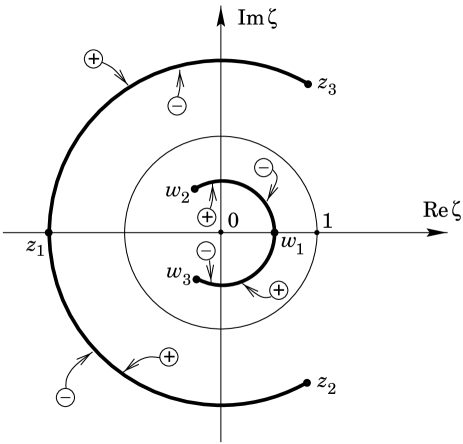
Figure 3: Branch cuts for the spectral curve of the tetrahedral 3-monopole

It is not hard to see that one obtains a compact Riemann surface of genus four when three copies of the Riemann sphere are identified along the branch cuts as specified in Figure 3. In fact, by identifying three copies of the upper or lower hemispheres along the pair of cuts as above, one obtains a torus with three discs removed; the circles of the boundary correspond to the equators of the spheres we started with. Gluing together the two surfaces obtained in this way along their boundaries gives a compact curve of genus four. This is sketched in Figure 4; the three circles shown project under $\pi|_{S}$ to the equator $E$ of $\mathbb{CP}^{1}$, and they will be referred to as the equators on a given sheet. We shall adopt the convention of drawing the paths as dash-dotted, dashed or dotted curves if they lie on sheets $1$, $2$ or $3$, respectively.

Figure 4: Spectral curve of the tetrahedral 3-monopole

Now we choose a canonical basis for $H_{1}(S,\mathbb{Z})\cong\mathbb{Z}^{\oplus 8}$ as in Figure 5. The first two $1$-cycles $a_{1}$ and $b_{1}$ are drawn close to the cut connecting the $z_{i}$’s so as to have the desired intersection number; for $a_{2}$ and $b_{2}$ we choose the equator on sheet 2 and a distorted meridian intersecting it as required; all the other intersections between these four $1$-cycles are zero. Then we act with the reality map $\tau$ on these cycles to get the other elements of the basis:

$$a_{3}:=\tau_{*}a_{2},\;\;a_{4}:=\tau_{*}a_{1},\;\;b_{3}:=-\tau_{*}b_{2},\;\;b_{4}:=-\tau_{*}b_{1}.$$ (42)

Our choice of branch cuts is such that $\tau$ sends cuts to cuts and hence maps a given sheet onto another sheet. It is easy to check that for $\zeta\in\mathbb{R}$, $\eta$ as given by (41) for $j=1$ also takes real values (cf equation (2)). We then conclude that sheet $1$ is invariant under $\tau$, while the other two sheets are interchanged. It follows that the second half of our homology basis is as drawn in Figure 5, and all the remaining intersection numbers for the elements in the basis are as required by (14).

Figure 5: The basis for $H_{1}(S,\mathbb{Z})$

Our chosen basis for $H^{0}(S,\Omega_{S}^{1})$ is

$$\Omega^{(1)}=\frac{d\zeta}{3\eta},\;\;\Omega^{(2)}=\frac{d\zeta}{3\eta^{2}},\;\;\Omega^{(3)}=\frac{\zeta d\zeta}{3\eta^{2}},\;\;\Omega^{(4)}=\frac{\zeta^{2}d\zeta}{3\eta^{2}}.$$ (43)

According to (31) these forms are pulled back by the reality structure as

$$\tau^{*}\Omega^{(1)}=-\overline{\Omega^{(1)}},\;\;\;\;\tau^{*}\Omega^{(2)}=\overline{\Omega^{(4)}},\;\;\;\;\tau^{*}\Omega^{(3)}=-\overline{\Omega^{(3)}},\;\;\;\;\tau^{*}\Omega^{(4)}=\overline{\Omega^{(2)}}.$$ (44)

We are now ready to compute the period matrix. The reality properties (42) and (44) imply that the periods around $a_{2}$, $a_{1}$, $b_{2}$ and $b_{1}$ determine those around $a_{3}$, $a_{4}$, $b_{3}$ and $b_{4}$, respectively. For example,

$$B_{23}=\oint_{-\tau_{*}b_{2}}\overline{\tau^{*}\Omega^{(4)}}=-\overline{\oint_{b_{2}}\Omega^{(4)}}=-\overline{B_{42}}.$$ (45)

This means that we only have to calculate half of the $32$ entries of the period matrix.

First we consider the periods around the equator $a_{2}$. Notice that $\zeta^{3}+5\sqrt{2}-\zeta^{-3}$ is invariant under the change of variable $\zeta\mapsto\omega\zeta$. So

$$A_{22}=-\frac{(1+\omega+\bar{\omega})}{3\alpha^{1/3}}\int_{1}^{\omega}\frac{d\zeta}{\zeta^{2}\left(\zeta^{3}+5\sqrt{2}-\zeta^{-3}\right)^{2/3}}=0$$

and similarly $A_{42}=0$. The two integrals $A_{12}$ and $A_{32}$ can be expressed in terms of the hypergeometric function ${}_{2}F_{1}$. Letting $F:={}_{2}F_{1}(\frac{1}{6},\frac{2}{3};1;-\frac{2}{25})$, we find

$$A_{12}=-\frac{2i\bar{\omega}}{3(5\sqrt{2}\alpha)^{1/3}}\int_{-\frac{\pi}{2}}^{\frac{\pi}{2}}\frac{du}{\left(1-\frac{i\sqrt{2}}{5}\sin u\right)^{1/3}}=-\frac{2\pi i\bar{\omega}F}{3\sqrt[3]{5}\sqrt[6]{2}\alpha^{1/3}}$$

and, using the relation (see [1], p. 559)

$${}_{2}F_{1}\left({\frac{1}{3}},{\frac{5}{6}};1;{-\frac{2}{25}}\right)=\frac{\sqrt[3]{5}}{\sqrt{3}}{\,}_{2}F_{1}\left({\frac{1}{6}},{\frac{2}{3}};1;{-\frac{2}{25}}\right),$$

we obtain

$$A_{32}=\frac{2i{\omega}}{3(5\sqrt{2}\alpha)^{2/3}}\int_{-\frac{\pi}{2}}^{\frac{\pi}{2}}\frac{du}{\left(1-\frac{i\sqrt{2}}{5}\sin u\right)^{2/3}}=\frac{2\pi i{\omega}F}{3\sqrt{3}\sqrt[3]{10}\alpha^{2/3}}.$$

Our choice of $a_{1}$ and $b_{1}$ implies that the periods around these two cycles are related by conjugation,

$$A_{i1}=\overline{B_{i1}}.$$

This follows from the fact that the paths $\pi\circ a_{1}$ and $\pi\circ b_{1}$ are complex conjugate, while

$$\overline{\eta_{2}(\zeta)}={\eta_{3}(\overline{\zeta})}$$

from the definition in (41).

There remain eight integrals to be calculated. By resorting to numerical integration, we have established that they are related to the periods around $a_{2}$ by simple numerical factors. The conclusion is that the two blocks $\mathbf{A}$ and $\mathbf{B}$ of the period matrix can be written as

$$\mathbf{A}=\begin{bmatrix}\displaystyle{\frac{2\pi F}{3\sqrt{3}\sqrt[3]{5}\sqrt[6]{2}\alpha^{1/3}}}&\displaystyle{-\frac{2\pi i\bar{\omega}F}{3\sqrt[3]{5}\sqrt[6]{2}\alpha^{1/3}}}&\displaystyle{-\frac{2\pi i\omega F}{3\sqrt[3]{5}\sqrt[6]{2}\alpha^{1/3}}}&\displaystyle{-\frac{2\pi F}{3\sqrt{3}\sqrt[3]{5}\sqrt[6]{2}\alpha^{1/3}}}\\[15.0pt] 0&0&0&\displaystyle{\frac{4\sqrt{2}\pi\bar{\omega}F}{9\sqrt[3]{10}\alpha^{2/3}}}\\[15.0pt] \displaystyle{\frac{2\pi F}{9\sqrt[3]{10}\alpha^{2/3}}}&\displaystyle{\frac{2\pi i\omega F}{3\sqrt{3}\sqrt[3]{10}\alpha^{2/3}}}&\displaystyle{\frac{2\pi i\bar{\omega}F}{3\sqrt{3}\sqrt[3]{10}\alpha^{2/3}}}&\displaystyle{-\frac{2\pi F}{9\sqrt[3]{10}\alpha^{2/3}}}\\[15.0pt] \displaystyle{\frac{4\sqrt{2}\pi\omega F}{9\sqrt[3]{10}\alpha^{2/3}}}&0&0&0\end{bmatrix}$$

and

$$\mathbf{B}=\begin{bmatrix}\displaystyle{\frac{2\pi F}{3\sqrt{3}\sqrt[3]{5}\sqrt[6]{2}\alpha^{1/3}}}&\displaystyle{-\frac{4\pi F}{3\sqrt{3}\sqrt[3]{5}\sqrt[6]{2}\alpha^{1/3}}}&\displaystyle{-\frac{4\pi F}{3\sqrt{3}\sqrt[3]{5}\sqrt[6]{2}\alpha^{1/3}}}&\displaystyle{\frac{2\pi F}{3\sqrt{3}\sqrt[3]{5}\sqrt[6]{2}\alpha^{1/3}}}\\[15.0pt] 0&\displaystyle{\frac{4\sqrt{2}\pi iF}{9\sqrt{3}\sqrt[3]{10}\alpha^{2/3}}}&\displaystyle{-\frac{4\sqrt{2}\pi iF}{9\sqrt{3}\sqrt[3]{10}\alpha^{2/3}}}&\displaystyle{-\frac{4\sqrt{2}\pi\omega F}{9\sqrt[3]{10}\alpha^{2/3}}}\\[15.0pt] \displaystyle{\frac{2\pi F}{9\sqrt[3]{10}\alpha^{2/3}}}&\displaystyle{-\frac{4\pi iF}{9\sqrt{3}\sqrt[3]{10}\alpha^{2/3}}}&\displaystyle{\frac{4\pi iF}{9\sqrt{3}\sqrt[3]{10}\alpha^{2/3}}}&\displaystyle{\frac{2\pi F}{9\sqrt[3]{10}\alpha^{2/3}}}\\[15.0pt] \displaystyle{\frac{4\sqrt{2}\pi\bar{\omega}F}{9\sqrt[3]{10}\alpha^{2/3}}}&\displaystyle{-\frac{4\sqrt{2}\pi iF}{9\sqrt{3}\sqrt[3]{10}\alpha^{2/3}}}&\displaystyle{\frac{4\sqrt{2}\pi iF}{9\sqrt{3}\sqrt[3]{10}\alpha^{2/3}}}&0\end{bmatrix}.$$

We have now all that is needed to determine $\alpha$ from the conditions (27). For a given $\alpha$, this is a system of eight real linear equations in eight (integer) unknowns. It has a solution given by

$$\mathbf{n}=\begin{bmatrix}0\\ 0\\ 0\\ 0\end{bmatrix},\;\;\;\;\;\mathbf{m}=m\begin{bmatrix}0\\ 1\\ 1\\ 0\end{bmatrix},$$

where $m$ satisfies

$$m=\frac{3\sqrt{3}\sqrt[3]{5}\sqrt[6]{2}\,\alpha^{1/3}}{4\pi F}.$$

Now $m$ must be either $1$ or $-1$ for $(\mathbf{m},\mathbf{n})$ to be primitive in $\mathbb{Z}^{\oplus 8}$. If we take $m=1$,

$$\alpha=\frac{32\sqrt{2}\pi^{3}F^{3}}{405\sqrt{3}},$$ (46)

while $m=-1$ reverses the sign of $\alpha$. The two solutions can be seen to be a rotation of each other by $\zeta\mapsto-\frac{1}{\zeta}$; to fix ideas, we take $\alpha$ positive from now on. It can be checked numerically that (46) agrees with the solution obtained in [9]. For our orientation of the spectral curve (40), the latter is given by

$$\alpha=\frac{\sqrt{2}}{3\sqrt{3}}\cdot\frac{\Gamma(\frac{1}{6})^{3}\Gamma(\frac{1}{3})^{3}}{48\sqrt{3}\pi^{3/2}}=\frac{\Gamma(\frac{1}{3})^{9}}{48\sqrt{6}\pi^{3}}.$$ (47)

In section 5.2, we use a change of variables projecting $S$ onto an elliptic curve to relate analytically the two results.

The special 1-cycle $c$ for the tetrahedral 3-monopole with $a$ positive is

$$c=b_{2}+b_{3}.$$ (48)

It is sketched on the Riemann sphere in Figure 6, after simplification using relations in homology — for example, the sum of the three equators with the same orientation is homologous to zero, which is clear from Figure 4. Clearly, it is not a combination of a lift of equators, since the projections of $b_{2}$ and $b_{3}$ enclose different branch points on the Riemann sphere. In the next section, it will be proved that $c$ is invariant under the tetrahedral group.

Figure 6: The special 1-cycle $c$ for the tetrahedral 3-monopole

5.2 Action of the tetrahedral group

The spectral curve $S$ defined by (40) admits an action of the tetrahedral group $\mathfrak{A}_{4}\subset SO(3)$ determined by $PSU(2)$ transformations on $\zeta$; the corresponding rotations are the symmetries of the tetrahedron drawn in Figure 2. This induces an action on $H_{1}(S,\mathbb{Z})$, which we now describe.

Recall that $\mathfrak{A}_{4}$ is generated by the 3-cycle $(123)$ and the double transposition $(12)(34)$. We represent these as the rotation by $\frac{2\pi}{3}$ about the direction defined by the top vertex $0$ of the tetrahedron in Figure 2,

$$R:\zeta\mapsto e^{\frac{2\pi i}{3}}\zeta,$$ (49)

and the rotation by $\pi$ around the axis connecting the edge midpoints $w_{1}$ and $z_{1}$,

$$T:\zeta\mapsto\frac{\sqrt{2}-\zeta}{1+\sqrt{2}\zeta},$$ (50)

respectively. Later, we will also be interested in another element of order two,

$$V=R\,TR^{\,2},$$ (51)

which corresponds to a rotation by $\pi$ about the axis connecting $w_{2}$ and $z_{2}$. We also denote by $R$, $T$ and $V$ the maps induced on $S$ by (49), (50) and (51).

On the complex plane, $R$ is of course just the rotation by $\frac{2\pi}{3}$ about the origin, while $T$ and $V$ are elliptic Möbius transformations of order two with $w_{1},z_{1}$ and $w_{2},z_{2}$ as fixed points, respectively. A way to visualize the action of $T$ or $V$ is to draw the (invariant) circles of Apollonius corresponding to the two fixed points; the other four branch points of $\pi|_{S}$ all lie on one of these circles and it is easy to verify that they are permuted as expected under the two transformations.

To describe the action of $\mathfrak{A}_{4}$ on $H_{1}(S,\mathbb{Z})$, we start by computing the matrices representing the generators $R$ and $T$. The effect of $R$ is easy to understand, since it leaves the three annuli over $C=\{\zeta:|w_{1}|<|\zeta|<|z_{1}|\}$ invariant. $T$ is harder to describe since it does not preserve the annuli, on which we can easily keep track of the sheet labels by using the expression (41) for $\eta_{j}(\zeta)$. But we can still use (41) when $\zeta$ is in the smaller region $C_{+}\cup C_{-}$, where

$$C_{\pm}:=\{\zeta\in C\cap T(C):\pm{\rm Im}\>\zeta>0\}$$

are mapped onto each other by $T$. Denoting by $C_{\pm,j}$ the intersection of $(\pi|_{S})^{-1}(C_{\pm})$ with sheet $j$, it can be concluded that $T$ sends $C_{\pm,j}$ to $C_{\mp,j\mp 1}$, where the labels are taken mod $3$. The sheet that contains the image under $R$ or $T$ of any point on $S$ can now be easily identified from these data and analytic continuation. In particular, we conclude that the 1-cycles in our basis for $H_{1}(S,\mathbb{Z})$ are mapped as shown in Figure 7.

Figure 7: The action of $R$ and $T$ on the basis of $H_{1}(S,\mathbb{Z})$

We can now use the perfect intersection pairing (14) to compute the matrices of the maps $R_{*}$ and $T_{*}$ induced on homology from the intersection numbers of the 1-cycles $a_{i}$ and $b_{i}$ with their images. Let $c_{i}:=a_{i}$ and $c_{4+i}:=b_{i}$ for $i=1,\ldots,4$. Defining

$$M_{ij}:=\sharp(R_{*}c_{i},c_{j}),\;\;\;\;\;N_{ij}:=\sharp(T_{*}c_{i},c_{j}),$$

we obtain the entries of the matrices $\mathbf{R}$ and $\mathbf{T}$ representing $R_{*}$ and $T_{*}$ as

$$R_{ij}=\sum_{k=1}^{8}J_{ik}M_{jk},\;\;\;\;T_{ij}=\sum_{k=1}^{8}J_{ik}N_{jk},$$

where, as in (30),

$$J_{ij}:=\sharp(c_{i},c_{j})=\begin{bmatrix}&\mathbf{1}_{4}\\ -\mathbf{1}_{4}&\end{bmatrix}_{ij}.$$

The intersection numbers $M_{ij}$ and $N_{ij}$ can be just read off from Figure 7, and we get

$$\mathbf{R}=\left[\begin{array}[]{cccc|cccc}0&0&0&0&-1&0&0&0\\ 0&1&0&0&-1&0&0&-1\\ 0&0&1&0&1&0&0&1\\ 0&0&0&0&0&0&0&1\\ \hline\cr 1&0&0&0&-1&-1&1&0\\ 0&0&0&0&0&1&0&0\\ 0&0&0&0&0&0&1&0\\ 0&0&0&-1&0&1&-1&-1\end{array}\right]$$

and

$$\mathbf{T}=\left[\begin{array}[]{cccc|cccc}-1&0&-1&0&0&0&0&0\\ 0&1&0&0&0&0&0&0\\ 0&0&1&0&0&0&0&0\\ 0&-1&0&-1&0&0&0&0\\ \hline\cr 0&1&0&0&-1&0&0&0\\ -1&0&-1&0&0&1&0&-1\\ 0&1&0&1&-1&0&1&0\\ 0&0&-1&0&0&0&0&-1\end{array}\right].$$

So the characters of the $\mathfrak{A}_{4}$ representation on 1-cycles are

$${\rm tr}\,\mathbf{1}_{8}=8,\;\;\;\;{\rm tr}\,\mathbf{R}=2={\rm tr}\,\mathbf{R}^{2},\;\;\;\;{\rm tr}\,\mathbf{T}=0,$$

and this shows that $H_{1}(S,\mathbb{C})$ splits as $\mathbf{1}^{\oplus 2}\oplus\mathbf{3}^{\oplus{2}}$. Another way to see this is to consider the action of $\mathfrak{A}_{4}$ by pull-back on the holomorphic 1-forms $\Omega^{(\ell)}$ by $R$ and $T$ and calculate the characters to conclude that $H_{0}(S,\Omega_{S}^{1})$ splits as $\mathbf{1}\oplus\mathbf{3}$ under $\mathfrak{A}_{4}$ (with $\Omega^{(1)}$ spanning the trivial singlet and being orthogonal to the triplet), and use Poincaré duality.

Using the matrices for $R_{*}$ and $T_{*}$, we can compute the projection $\boldsymbol{\Pi}$ onto the subspace $\mathbf{1}^{\oplus 2}\subset H_{1}(S,\mathbb{C})$ as

$$\boldsymbol{\Pi}=\frac{1}{|\mathfrak{A}_{4}|}\sum_{\sigma\in\mathfrak{A}_{4}}\boldsymbol{\sigma}=\frac{1}{4}\left[\begin{array}[]{cccc|cccc}0&-1&-1&0&0&0&0&0\\ 0&2&2&0&0&0&0&0\\ 0&2&2&0&0&0&0&0\\ 0&-1&-1&0&0&0&0&0\\ \hline\cr 0&1&1&0&0&0&0&0\\ -1&0&-3&1&-1&2&2&-1\\ -1&3&0&1&-1&2&2&-1\\ 0&-1&-1&0&0&0&0&0\end{array}\right].$$

The range of this matrix is spanned by

$$\begin{bmatrix}0&0&0&0&0&1&1&0\end{bmatrix}^{t}\;\;\;\;\;{\rm and}\;\;\;\;\;\begin{bmatrix}2&-4&-4&2&-2&3&-3&2\end{bmatrix}^{t},$$ (52)

so we conclude that the special cycle $c$ given in (48) is invariant under the action of $\mathfrak{A}_{4}$. Notice that in (52) the first vector is antisymmetric whereas the second is symmetric under reality.

We can explore the action of the Vierergruppe $D_{2}\subset\mathfrak{A}_{4}$ generated by the two elements $T$ and $V$ to express the value $\alpha$ given by (46) in terms of elliptic integrals, as in [9]. The actions of both $T$ and $V$ are much easier to describe in an alternative orientation of the monopole, obtained by rotation of (40) under

$$\zeta\mapsto\frac{(z_{3}-z_{1})(\zeta-w_{1})}{(z_{3}-w_{1})(\zeta-z_{1})}.$$

Then the spectral curve is taken to the form

$$\eta^{3}+\frac{3\sqrt{3}}{\sqrt{2}}\alpha i\zeta(\zeta^{4}-1)=0,$$ (53)

which can be described as a covering of $\mathbb{CP}^{1}$ with branch points at $0$, $\pm 1$, $\pm i$ and $\infty$. In this configuration, $T$ is just $\zeta\mapsto-\zeta$, while $V$ is $\zeta\mapsto-\frac{1}{\zeta}$. The map

$$p:\zeta\mapsto\frac{1}{2}\left(\zeta^{2}+\frac{1}{\zeta^{2}}\right)=:z$$

identifies points in the same orbit of $D_{2}$, having the first quadrant as fundamental region. Under the map induced on $T^{\prime}\mathbb{CP}^{1}$ by $p$, the spectral curve (53) goes to

$$w^{3}+24\sqrt{6}\alpha i(z^{2}-1)^{2}=0,$$

which is a torus by the Riemann–Hurwitz formula and corresponds to the quotient $S/D_{2}$. The two pairs of branch cuts on the original Riemann sphere are both identified with a cut connecting the new branch points $1$, $\infty$ and $-1$ along the real axis. With some care, it can be seen that the image of the 1-cycle $c$ in (48) can be identified with a cycle going four times along the imaginary axis in the negative direction, on the sheet containing the point $(w,z)=(2\sqrt[6]{2}\sqrt{3}\alpha^{1/3}i,0)$. On the other hand, it is easy to see that the 1-form $\Omega^{(1)}$ is given by the same expression in the new orientation, and

$$p^{*}\left(\frac{dz}{3w}\right)=\frac{d\zeta}{3\eta}=\Omega^{(1)}.$$

Thus we can write

$$\oint_{c}\Omega^{(1)}=\oint_{p_{*}c}\frac{dz}{3w}=4\int_{i\infty}^{-i\infty}\frac{dz}{6\sqrt[6]{2}\sqrt{3}\omega\alpha^{1/3}\left(-i(z^{2}-1)^{2}\right)^{1/3}}$$

and this can be reduced to an elliptic integral, yielding

$$-\frac{\Gamma(\frac{1}{3})^{3}}{\sqrt{6}\pi\alpha^{1/3}}.$$

Now this has to be equal to $-2$ by (26). Thus we get

$$\alpha=\frac{\Gamma(\frac{1}{3})^{9}}{48\sqrt{6}\pi^{3}}$$

in agreement with (47).

6 Discussion

The version of the Ercolani–Sinha constraints that we derived in section 3 generalises the Corrigan–Goddard conditions to all monopoles with a nonsingular spectral curve. An interesting aspect is the existence of a distinguished 1-cycle $c$ on the spectral curve. The premises in the Corrigan–Goddard approach lead to the constraint (39) for $c$, but their conditions are otherwise equivalent to equation (24). In section 5, we have applied (24) to rederive the scale parameter $\alpha$ in the spectral curve of the tetrahedrally symmetric monopole of charge 3. We also verified that this monopole provides an example where our condition (24) can be satisfied but those of Corrigan and Goddard are not.

Let us make some remarks about the nature of the special 1-cycle $c$. Given a nonsingular spectral curve $S$ in $\mathbb{T}$, $c$ is uniquely determined as the solution to equation (24); we have established that it is always antisymmetric under the real structure. Moreover, although the left-hand side of (24) depends on the spatial orientation of the monopole, $c$ remains constant along the $SO(3)$ orbit of $S$ in the moduli space ${\cal N}_{k}$. In fact, its components in a given homology basis are integer solutions to a linear equation and cannot change when the spectral curve is rotated, since the period matrix occurring in (15) never becomes singular. This argument applies to more general deformations in ${\cal N}_{k}$ that do not pass through monopoles with a singular spectral curve. It also implies that $c$ has to be invariant under any rotational symmetry of the spectral curve, and this imposes further restrictions — for example, in the case of the tetrahedrally symmetric 3-monopole that we studied in section 5, this consideration together with the $\tau$-antisymmetry completely determines $c$ up to sign.

As implied in [4], the components of the 1-cycle $c$ are the characteristics of the line bundle $L^{2}|_{S}$ and can thus be interpreted as giving the direction of the linear flow determined by Nahm’s equations on the Jacobian of the spectral curve $S$. Another interpretation for $c$ is afforded by equation (16). Recall that the triviality of $L^{2}|_{S}$ provides for two nowhere vanishing functions $f_{0}$ and $f_{1}$ on the open sets $U_{0}\cap S$ and $U_{1}\cap S$. We may wonder whether we can define logarithms of these functions. And of course the answer is no: the nonzero components of $c$ correspond to nontrivial periods of both $d\,{\rm log}f_{0}$ and $d\,{\rm log}f_{1}$, and so they cannot be exact 1-forms. To define the logarithms, one should eliminate the 1-cycles correponding to the nonzero periods, by cutting $S$ along their conjugate homology 1-cyles in the canonical basis (14). But we can see from (17) that this is equivalent to cutting $S$ along $c$. The Riemann surface of ${\rm log}f_{0}$ or ${\rm log}f_{1}$ is then obtained from the cut surfaces $U_{0}\cap S$ or $U_{1}\cap S$ by analytic continuation across the cuts, and this yields an infinite cover of the original open sets. So we may regard $c$ as a topological obstruction to defining the logarithms of the nowhere vanishing functions $f_{0}$ and $f_{1}$ on the spectral curve punctured at the points lying over $\zeta=\infty$ and $\zeta=0$, respectively.

We should emphasise that the Ercolani–Sinha algorithm is still not sufficient to ensure smoothness of the fields if $k>2$, since it does not include the condition (7). The family of nonsingular spectral curves of monopoles has codimension zero in the family of real curves in $|{\cal O}(2k)|$ satisfying equation (24), but the inclusion is proper in general. For example, it can be shown that the icosahedrally symmetric curve

$$\eta^{6}+\alpha\zeta(\zeta^{10}+11\zeta^{5}-1)=0$$ (54)

satisfies (24) for some constant $\alpha$, but not (7); this follows from the conclusion in [9] that there is no 6-monopole with icosahedral symmetry. It is known [11] that an icosahedrally symmetric monopole of charge $7$ exists, and its spectral curve is reducible to a projective line and a smooth genus $25$ curve of the form (54), with $\alpha=\frac{3^{3}\Gamma(\frac{1}{3})^{18}}{2^{8}\pi^{6}}$.

An interesting question is to understand how (24) degenerates when a spectral curve becomes singular. Some singularities arise by imposing interesting symmetries on the monopoles, as in the case of the axially symmetric monopoles that we have mentioned already. We may expect that the condition still holds for other singular spectral curves, but it is not clear how the 1-cycle $c$ is to be determined in general.

Acknowledgements

We thank Roger Bielawski for advice. CJH thanks Fitzwilliam College, Cambridge, for a research fellowship. NMR is supported by Fundação para a Ciência e a Tecnologia, Portugal, through the research grant BD/15939/98.

References

- [1] Abramowitz, M. and Stegun, I. A.: Handbook of Mathematical Functions. National Bureau of Standards, 1965
- [2] Atiyah, M. F. and Hitchin, N. J.: The Geometry and Dynamics of Magnetic Monopoles. Princeton University Press, 1988
- [3] Corrigan, E. and Goddard, P.: An Monopole Solution with Degrees of Freedom. Commun. Math. Phys. 80, 575–587 (1981)
- [4] Ercolani, N. and Sinha, A.: Monopoles and Baker Functions. Commun. Math. Phys. 125, 385–416 (1989)
- [5] Forgács, P., Horváth, Z. and Palla, L.: Finitely Separated Multimonopoles Generated as Solitons. Phys. Lett. 109B, 200–204 (1982)
- [6] Griffiths, P. and Harris, J.: Principles of Algebraic Geometry. Wiley, 1978
- [7] Hitchin, N. J.: Monopoles and Geodesics. Commun. Math. Phys. 83, 579–602 (1982)
- [8] Hitchin, N. J.: On the Construction of Monopoles. Commun. Math. Phys. 89, 145–190 (1983)
- [9] Hitchin, N. J., Manton, N. S. and Murray, M. K.: Symmetric Monopoles. Nonlinearity 8, 661–692 (1995); dg-ga/9503016
- [10] Houghton, C. J. and Sutcliffe, P. M.: Tetrahedral and Cubic Monopoles. Commun. Math. Phys. 180, 343–361 (1996); hep-th/9601146
- [11] Houghton, C. J. and Sutcliffe, P. M.: Octahedral and Dodecahedral Monopoles. Nonlinearity 9, 385–401 (1996); hep-th/9601147
- [12] Hurtubise, J.: Monopoles of Charge . Commun. Math. Phys. 92, 195–202 (1983)
- [13] O’Raifeartaigh, L., Rouhani, S. and Singh, L. P.: Explicit Solution of the Corrigan–Goddard Conditions for Monopoles for Small Values of the Parameters. Phys. Lett. 112B, 369–372 (1982)
- [14] Sutcliffe, P. M.: BPS Monopoles. Int. J. Mod. Phys. A 12, 4663–4705 (1997); hep-th/9707009
- [15] Ward, R. S.: A Yang–Mills–Higgs Monopole of Charge . Commun. Math. Phys. 79, 317–325 (1981)