More $\mathsf{D}$-branes in the Nappi–Witten background

Abstract.

We re-examine the problem of determining the possible $\mathsf{D}$-branes in the Nappi–Witten background. In addition to the known branes, we find that there are also $\mathsf{D}$-instantons, flat euclidean $\mathsf{D}$-strings and curved $\mathsf{D}$-membranes admitting parallel spinors, all of which can be interpreted as (twisted) conjugacy classes in the Nappi–Witten group.

1. Introduction and motivation

$\mathsf{D}$-branes have played a central role in many of the fascinating developments in string theory in the last few years. They have proved particularly versatile in bridging the gap between gauge theory and gravity. This is due to the fact that they admit two very different descriptions: as stable solutions of type II supergravity on the one hand, and as boundary conditions for open strings on the other. Despite the fact that both descriptions play equally important roles in the gravity/gauge theory correspondence, the present state of our knowledge displays a conspicuous lack of symmetry. Whereas there has been much progress in constructing $\mathsf{D}$-brane-type solutions to type II supergravity, it is only in very few cases that we can actually ascertain that these solutions describe possible boundary conditions for open strings. In particular, very little is known about $\mathsf{D}$-branes (in the sense of open string boundary conditions) in nontrivial backgrounds, e.g., in curved space. This mirrors the fact that whereas one can write down many supergravity vacua, it is not clear how to describe string propagation on many of them. It therefore might seem unreasonable to expect a stringy description of a $\mathsf{D}$-brane solution on a background for which string propagation (without branes) cannot be adequately described. By the same token, it is not unreasonable to expect that we should be able to understand $\mathsf{D}$-branes in those backgrounds for which a conformal field theory can be written down. Such backgrounds include flat spaces, orbifolds, toroidal and Calabi–Yau compactifications, and WZW and coset models. In many of these cases, $\mathsf{D}$-branes are fairly well understood from both geometric and conformal field theoretic points of view, but in some cases (e.g., the WZW model) a lot less is known than one might expect.

The purpose of the present paper is to re-examine the problem of determining the possible conformal invariant Dirichlet boundary conditions in a WZW model from a geometric perspective, and to illustrate the results in the case of the WZW model associated to the Nappi–Witten group [5]. This string background is privileged in that it can be treated exactly as a conformal field theory, and the geometry is also simple enough to be studied classically. It also displays, as we shall see, many of the features of $\mathsf{D}$-branes present in general WZW models. The analysis complements the work in [8] in that we study a different type of gluing conditions for the chiral currents.

There is growing body of literature on the subject of boundary conditions in WZW models, and we will not attempt to list all relevant papers here, except for those which have a direct relation to the present one. A fuller comparative discussion of the literature can be found in [6], which explains the geometric interpretation of the gluing conditions on which this paper is based.

This note is organised as follows. In Section 2 we discuss boundary conditions for WZW models and their relation to the more familiar gluing conditions on the chiral currents. The approach here follows the one in [6]. In contrast with that paper, we restrict ourselves to the case of gluing conditions given by an automorphism. The associated boundary conditions are then those associated to conjugacy classes and twisted generalisations thereof. In Section 3 we illustrate these results to the Nappi–Witten group and we determine its (twisted) conjugacy classes, identifying those which can be interpreted as $\mathsf{D}$-branes. We will see that among these classes one finds curved membranes, flat euclidean strings and instantons. In Section 4 we summarise the results of the paper.

2. $\mathsf{D}$-branes in WZW models

The WZW model is the theory of harmonic maps $g:\Sigma\to G$ from a two-dimensional worldsheet $\Sigma$ to a Lie group $G$ possessing a bi-invariant metric. This induces on the Lie algebra $\mathfrak{g}$ of $G$ an invariant scalar product. Let the worldsheet have boundary $\partial\Sigma$. In the simplest case, $\mathsf{D}$-branes will correspond to certain submanifolds $B\subset G$ which can be used as boundary conditions; that is, such that the map $g$ takes the boundary of the worldsheet to $B$. In other words, in the presence of a $\mathsf{D}$-brane, admissible field configurations are those maps $g:\Sigma\to G$ such that $g:\partial\Sigma\to B$. Not all submanifolds $B\subset G$ are allowed: a consistent boundary condition must preserve conformal invariance.

2.1. Boundary conditions

The conformal symmetry of the WZW model is a consequence of the affine symmetry

$$g(z,\bar{z})\mapsto\Omega(z)g(z,\bar{z})\bar{\Omega}(\bar{z})^{-1}~{},$$

where $\Omega(z)$ and $\bar{\Omega}(\bar{z})$ are independent maps from $\Sigma$ to $G$ depending holomorphically and anti-holomorphically, respectively, on the complex coordinate. One way to guarantee conformal invariance of a boundary condition is therefore to preserve a large enough subgroup of the affine symmetry.

Let us fix one boundary component and choose a local parametrisation of the worldsheet for which the boundary component in question coincides with the real axis $z=\bar{z}$. Then at the boundary the affine symmetry becomes

$$g\bigr{|}_{\partial\Sigma}\mapsto\Omega(z)g\bigr{|}_{\partial\Sigma}\bar{\Omega}(z)^{-1}~{}.$$

It is easy to envisage submanifolds $B\subset G$ which preserve some of the affine symmetry; although proving the conformal invariance of the corresponding boundary conditions might be much more difficult. We will concentrate here on boundary conditions such that $B$ is a (twisted) conjugacy class, as this will be born out by our analysis of the geometry associated to certain gluing conditions.

Let $G$ be a connected Lie group and $g_{0}\in G$ an element. Let $C(g_{0})$ denote the conjugacy class of the element $g_{0}$, defined as the subset of $G$ with the following elements:

$$C(g_{0}):=\left\{gg_{0}g^{-1}\mid g\in G\right\}~{}.$$

The conjugacy class of an element $g_{0}$ is therefore the orbit of that element under the adjoint action of the group: $\mathrm{Ad}_{g}:G\to G$, defined by $\mathrm{Ad}_{g}(g_{0})=gg_{0}g^{-1}$. Each conjugacy class is a connected submanifold of $G$. Since every element $g_{0}$ belongs to one and only one conjugacy class, $G$ is foliated by its conjugacy classes. The leaves of the foliation need not all have the same topology; in other words, the foliation need not be a fibration.

For compact simple groups a well-known result says that every element is conjugate to some maximal torus $\mathbb{T}$. The Weyl group $W=N(\mathbb{T})/\mathbb{T}$ further relates elements of the maximal torus. Therefore the conjugacy classes are parametrised by the quotient $\mathbb{T}/W$ of a maximal torus by the Weyl group. For example, for $G=\mathrm{SU}(2)$, the conjugacy classes are parametrised by $S^{1}/\mathbb{Z}_{2}$, which we can understand as the interval $\theta\in[0,\pi]$. The conjugacy classes corresponding to $\theta=0,\pi$ are points, corresponding to the elements in the centre of $\mathrm{SU}(2)$: $\pm\mathbb{1}$, whereas the classes corresponding to $\theta\in(0,\pi)$ are spheres. If we picture $\mathrm{SU}(2)$, which is homeomorphic to the 3-sphere, as the one-point compactification of $\mathbb{R}^{3}$ where the sphere at infinity is collapsed to a point, the foliation of $\mathrm{SU}(2)$ by its conjugacy classes coincides with the standard foliation of $\mathbb{R}^{3}$ by 2-spheres with two degenerate spheres at the origin and at infinity. Because of the degeneration of the limiting spheres the foliation is not a fibration. This is not surprising, since $S^{3}$ is a circle bundle over $S^{2}$ and not a sphere bundle over $S^{1}$.

For noncompact groups the problem is more subtle since there is no longer a notion of maximal torus, even in the semisimple case. In the absence of a general theory, one has to treat each case independently. For example, the conjugacy classes of $\mathrm{SL}(2,\mathbb{R})$ can be found in [7], in the context of $\mathsf{D}$-branes on $\mathrm{AdS}_{3}$. In this paper we will determine the conjugacy classes of the noncompact nonreductive Lie group $\EuScript{N}$ introduced by Nappi and Witten in [5] and which we term the Nappi–Witten group.

The boundary conditions associated with conjugacy classes preserve an infinite-dimensional affine symmetry

$$g\bigr{|}_{\partial\Sigma}\mapsto\Omega(z)g\bigr{|}_{\partial\Sigma}\bar{\Omega}(z)^{-1}~{},$$ (1)

where now $\bar{\Omega}=\Omega$ at the boundary, but otherwise arbitrary.

A similar situation obtains in the case of boundary conditions which say that $B\subset G$ is a shifted conjugacy class: $B=h\,C$ or $B=C\,h$, where $h\in G$ and $C$ is a conjugacy class. This also respects the affine symmetry in (1), but acting on $h^{-1}g$ and $gh^{-1}$ respectively.

A way to generalise this situation is to consider twisted conjugacy classes. Every automorphism $r$ of the group gives rise to a twisted version of conjugacy classes, by considering the orbit of a group element $h$, say, under the twisted conjugation $h\mapsto ghr(g)^{-1}$. If the automorphism is inner, so that there is a group element $k$ such that $r(g)=kgk^{-1}$, then the orbit under the twisted conjugation is simply the shifted conjugacy class $k^{-1}C(gk)$; however when the automorphism is not inner, the orbits are quite different, as we will see below in the case of the Nappi–Witten group. These boundary conditions are also preserved by the infinite-dimensional affine symmetry given by (1), but where now $\bar{\Omega}=r(\Omega)$ at the boundary.

We will not attempt here to prove directly that all these boundary conditions preserve conformal invariance. One may argue that these boundary conditions seem reasonable because in the more familiar case of free fields, which we can think as an abelian WZW model, $\mathsf{D}$-branes are essentially points or planes, which can be interpreted group-theoretically as (twisted) conjugacy classes. Instead we will start from the gluing conditions satisfied by the chiral currents and under some natural assumptions recover the above boundary conditions.

2.2. Gluing conditions

In the same way as the conformal invariance of the WZW model is most easily proven using the infinite-dimensional affine symmetry obeyed by the currents, determining whether a boundary condition preserves conformal invariance is most easily achieved by deriving from it a condition in terms of the chiral currents.

In the algebraic approach to the WZW model, the fundamental dynamical variables are the affine currents

$$J(z)=-\partial g\,g^{-1}\qquad\text{and}\qquad\bar{J}(\bar{z})=g^{-1}\,\bar{\partial}g~{},$$

where $g=g(z,\bar{z})$. The dynamic content of the WZW model is encoded in the (anti-)holomorphicity of these currents. These currents are Lie algebra valued $(1,0)$- and $(0,1)$-forms on the worldsheet. The sign is chosen so that $J(z)$ and $\bar{J}(\bar{z})$ obey isomorphic affine algebras.

In this approach, boundary conditions are expressed as gluing conditions on the chiral currents. Let $R:\mathfrak{g}\to\mathfrak{g}$ denote an invertible linear map in the Lie algebra. At this moment we are not assuming any further properties of $R$. By a gluing condition we mean a relation of the form

$$\bar{J}(\bar{z})\bigr{|}_{\partial\Sigma}=RJ(z)\bigr{|}_{\partial\Sigma}~{}.$$ (2)

The fundamental requirement of a gluing condition is that it should preserve the conformal algebra at the boundary. In the WZW model, the Virasoro generators are made out of the chiral currents via the Sugawara construction, which takes the form

$$T(z)=\left<J(z),J(z)\right>\qquad\text{and}\qquad\bar{T}(\bar{z})=\left<\bar{J}(\bar{z}),\bar{J}(\bar{z})\right>~{},$$

where $\left<-,-\right>$ is a nondegenerate invariant scalar product in the Lie algebra $\mathfrak{g}$. Conformal invariance then dictates that $R$ should be an isometry of this scalar product. We will see below that under some further assumptions it is natural to demand that $R$ be a Lie algebra automorphism.

It should be mentioned that the map $R$ need not be constant, it could depend on the point $g\in G$; in other words, $R$ could be a function from the group $G$ to the group of isometries of $\mathfrak{g}$. Indeed, as shown in [8] via a $\sigma$-model analysis of the Neumann boundary conditions, in order to obtain a $\mathsf{D}$-brane which fills the whole group manifold (at least in the case of a noncompact group), one needs to impose a gluing condition with a nonconstant $R$. The implicit restriction to constant $R$ has no conceptual basis; it is simply a practical one, since it is not known in general how to work quantum-mechanically with the field $g$, but only with the chiral currents.

2.3. The geometry of the gluing conditions

The geometry of a $\mathsf{D}$-brane is encoded in the boundary conditions that the fields satisfy. Since the relation between the gluing conditions and boundary conditions is in most cases not straightforward, therein lies the major difficulty in the study of $\mathsf{D}$-branes on WZW models. One way to understand where the difficulty lies is to notice that the gluing conditions relate currents which take values in the Lie algebra, equivalently in the tangent space to the Lie group at the identity; whereas in order to derive any geometric information about the $\mathsf{D}$-brane what one needs are local conditions on the map $g:\Sigma\to G$ at the boundary of the worldsheet, which need not be mapped anywhere near the identity in the group. This complication is absent for an abelian group, since the currents are directly related to the coordinates; but for a nonabelian group the relationship between the gluing conditions and the boundary conditions is not totally understood. In what follows we will present a natural class of solutions related to (twisted) conjugacy classes, but as shown in [8, 7, 6] these are not the only possible solutions.

Let us start by writing down the gluing conditions (2) in terms of the map $g:\Sigma\to G$:

$$g^{-1}\bar{\partial}g=-R(\partial gg^{-1})~{},$$

where in this and in many of the following equations we are implicitly evaluating both sides of the equation on the boundary. This relation is a linear equation in the Lie algebra, which we identify with the tangent space to the Lie group at the identity. We can translate it to a linear equation at the point $g$:

$$\bar{\partial}g=-gR(\partial gg^{-1})~{},$$

where we have abused notation slightly and written the differentials of left- and right-multiplication as left and right multiplication by $g$, as for matrix groups. Introducing $\lambda$ and $\rho$ as the differential maps associated to left- and right-translations, respectively, we can rewrite this equation in a more invariant form as follows:

$$\bar{\partial}g=-(\lambda_{g}\circ R\circ\rho_{g}^{-1})\,\partial g~{}.$$ (3)

We seek to interpret this condition as defining a boundary condition of the form $g:\partial\Sigma\to B$ where $B\subset G$ is a submanifold. We will assume that in addition $B$ is nondegenerate, so that the bi-invariant metric on $G$ restricts non-degenerately to $B$. We believe this assumption to be physically reasonable. Let us remark that the bi-invariant metric on $G$ is the one induced by the invariant scalar product in the Lie algebra which is used in the Sugawara construction. As remarked earlier this need not agree with, or be in the same conformal class as, the metric appearing in the WZW lagrangian and hence in the operator product algebra of the chiral currents.

The assumption on the submanifold $B\subset G$ says that at any point $g\in B$ one has the following orthogonal decomposition of the tangent space to $G$:

$$T_{g}G=T_{g}B\oplus T_{g}B^{\perp}~{}.$$

We will let ^⟂ denote the orthogonal projection $T_{g}G\to T_{g}B^{\perp}$ along $T_{g}B$. In the open string picture, a (Dirichlet) boundary condition $g:\partial\Sigma\to B$ says that the normal component of the tangential derivative along the boundary vanishes, whence

$$(\bar{\partial}g)^{\perp}=-(\partial g)^{\perp}~{}.$$ (4)

Because of the bi-invariance of the metric and the fact that $R$ is an isometry, the linear map $(\lambda_{g}\circ R\circ\rho_{g}^{-1})$ respects the above orthogonal decomposition, whence the normal component of equation (3) together with (4) implies that

$$(\mathbb{1}-\lambda_{g}\circ R\circ\rho_{g}^{-1})(\partial g)^{\perp}=0~{}.$$

Since $\partial g$ is arbitrary on the boundary, this is obeyed by all normal vectors to $B$ at $g$, and hence defines what it means for a vector to be normal to $B$. This in turn will tell us what it means for a vector to be tangent to $B$.

The above equation says that a vector $\eta\in T_{g}G$ is normal to $B$ if and only if it belongs to the kernel of the linear map

$$(\mathbb{1}-\lambda_{g}\circ R\circ\rho_{g}^{-1}):T_{g}G\to T_{g}G~{}.$$

In other words,

$$T_{g}B^{\perp}=\ker(\mathbb{1}-\lambda_{g}\circ R\circ\rho_{g}^{-1})~{}.$$

Hence the tangent space $T_{g}B$ to $B$, being defined as the orthogonal complement of $T_{g}B^{\perp}$, is then the image of the adjoint of the above linear map

$$T_{g}B=T_{g}B^{\perp\perp}=\left[\ker(\mathbb{1}-\lambda_{g}\circ R\circ\rho_{g}^{-1})\right]^{\perp}=\mathrm{im}(\mathbb{1}-\lambda_{g}\circ R\circ\rho_{g}^{-1})^{\dagger}~{},$$

where

$$(\mathbb{1}-\lambda_{g}\circ R\circ\rho_{g}^{-1})^{\dagger}=\mathbb{1}-(\lambda_{g}\circ R\circ\rho_{g}^{-1})^{\dagger}\\ =\mathbb{1}-(\lambda_{g}\circ R\circ\rho_{g}^{-1})^{-1}=\mathbb{1}-\rho_{g}\circ R^{-1}\circ\lambda_{g}^{-1}~{},$$

where we have used the fact that $(\lambda_{g}\circ R\circ\rho_{g}^{-1})$ is an isometry, whence its adjoint is its inverse. In other words, the tangent space $T_{g}B$ to $B$ at $g$ is made out of vectors of the form

$$\xi-R^{-1}(g^{-1}\xi)g$$

for any $\xi\in T_{g}G$. Now, the tangent vectors $\xi$ can be put in one-to-one correspondence with vectors $X$ in the Lie algebra via the relation: $\xi=-gR(X)$. Therefore $T_{g}B$ consists of vectors of the form

$$Xg-gR(X)\qquad\text{for $X\in\mathfrak{g}$.}$$

There is one further condition that we have to impose. Since $B\subset G$ is a submanifold, its tangent vectors span an integrable distribution (in the sense of Frobenius); that is, the Lie bracket of two tangent vectors should again be a tangent vector. In other words, one must impose that

$$[Xg-gR(X),Yg-gR(Y)]=Zg-gR(Z)\quad\text{for some $Z\in\mathfrak{g}$.}$$ (5)

To compute the above Lie bracket we notice that left-invariant vector fields generate right-translations, which are anti-homomorphisms, whereas right-invariant vector fields generate left-translations, which are homomorphisms, and that left- and right-translations commute. Therefore, one computes

$$[Xg-gR(X),Yg-gR(Y)]=[XY]g-g[R(X)R(Y)]~{}.$$

Comparing with the right-hand side of equation (5) we see that

$$[XY]g-g[R(X)R(Y)]=Zg-gR(Z)\qquad\text{for some $Z\in\mathfrak{g}$.}$$

A natural solution is $Z=[XY]$ and hence $[R(X)R(Y)]=R([XY])$, so that $R$ is an automorphism; but it is important to realise that, since there is no unique way of decomposing a vector field into the sum of a left- and a right-invariant vector fields, this is not the only solution. Indeed, as evidenced by some of the results in [8, 7, 6], there are conformally invariant boundary conditions in WZW models for which $R$ is not an automorphism.

For the purposes of this paper we will however assume that $R$ is an automorphism, and discuss the resulting boundary conditions.

Let us offer two remarks:

• An automorphism $R$ leaves invariant the Killing form and hence if it is an isometry with respect to the scalar product in the Sugawara construction it will also be an isometry with respect to the scalar product appearing in the WZW lagrangian or in the operator product algebra of the chiral currents; and

• Taking $R$ to be automorphism forces $B$ to be a submanifold. This means that in order to describe configurations of intersecting branes, for example, where $B$ is the union of two submanifolds, one is forced to consider gluing conditions where $R$ is not an automorphism.

2.4. $\mathsf{D}$-branes and (twisted) conjugacy classes

We assume then that $R$ is an automorphism, so that the submanifold $B\subset G$ defining the boundary conditions is such that its tangent vectors at $g$ are all of the form $Xg-gR(X)$ for some $X\in\mathfrak{g}$. Such a vector is tangent to the following curve through $g$:

$$\gamma_{X}(t)=e^{tX}ge^{-tR(X)}~{}.$$ (6)

Let us define the map $r:G\to G$ by

$$r\left(e^{tX}\right)=e^{tR(X)}~{},$$

for small enough $t$ and for all $X\in\mathfrak{g}$. Since we assume that the group is connected, $r$ extends to a Lie group automorphism. It is moreover clear that $r$ is an isometry relative to the bi-invariant metric on the Lie group provided that $R$ preserves the scalar product in the Lie algebra. Therefore the curves described by (6) correspond to curves on the orbit of the point $g$ under the twisted adjoint action of the group: $\mathrm{Ad}^{r}(h)g:=hgr(h)^{-1}$, and hence $B$ can be identified with the orbit of $g$ under such an action:

$$B=C_{r}(g)=\left\{hgr(h)^{-1}\mid h\in G\right\}~{}.$$

We call these orbits twisted conjugacy classes, since they reduce to conjugacy classes when $r$ is the identity.

In contrast to the case of conjugacy classes, the twisted adjoint action does not preserve the group multiplication in general. Nevertheless, the twisted conjugacy class $C_{r}(g)$ is again a homogeneous space

$$C_{r}(g)\cong G/H_{r}(g)~{},$$

where $H_{r}(g)\subset G$ is now the isotropy subgroup of the element $g$:

$$H_{r}(g):=\left\{h\in G\mid hg=gr(h)\right\}~{}.$$

When $R$, and hence $r$, is the identity map, then $B$ agrees with the conjugacy class of the element $g$. The result that conjugacy classes could appear as $\mathsf{D}$-branes appeared for the first time in [1]. In [7] (see also [6]) it was further shown that in the case where $R$ is an inner automorphism, say $R=\mathrm{Ad}_{h}$ for some fixed group element $h$, the gluing condition (2) reads

$$-\partial gg^{-1}=hg^{-1}\bar{\partial}gh^{-1}~{},$$ (7)

which is equivalent to

$$-\partial\tilde{g}\tilde{g}^{-1}=\tilde{g}^{-1}\bar{\partial}\tilde{g}~{},$$

for $\tilde{g}=gh^{-1}$. This gluing condition therefore implies the boundary condition $\tilde{g}:\partial\Sigma\to C$, where $C$ is a conjugacy class; or equivalently $g:\partial\Sigma\to Ch$, where $Ch$ is the right-translate by $h$ of the conjugacy class $C$. Notice that $Ch=hC$ so that there is no ambiguity had we chosen to rewrite the gluing condition in terms of $h^{-1}g$.

More generally two automorphisms which are related by an inner automorphism give rise to twisted conjugacy classes which are translated relative to each other:

$$C_{r\circ\mathrm{Ad}_{h}}(g)=C_{r}(gr(h))r(h)^{-1}\qquad\text{and}\qquad C_{\mathrm{Ad}_{h}\circ r}(g)=C_{r}(gh)h^{-1}~{}.$$

This suggests that we organise the possible boundary conditions according to the group of (metric-preserving) outer automorphisms. Indeed, let $\mathrm{Aut}_{o}(G)$ denote the group of metric-preserving automorphisms of $G$ and let $\mathrm{Inn}_{o}(G)\subset\mathrm{Aut}_{o}(G)$ denote the invariant subgroup corresponding to those automorphisms which are inner. Then one can define the factor group

$$\mathrm{Out}_{o}(G):=\mathrm{Aut}_{o}(G)/\mathrm{Inn}_{o}(G)~{},$$

of metric-preserving outer automorphisms. Elements of $\mathrm{Out}_{o}(G)$ are equivalence classes of metric-preserving automorphisms of $G$: two such automorphisms being equivalent if they are related by an inner automorphism. To each element of $\mathrm{Out}_{o}(G)$ we can associate an equivalence classes of $\mathsf{D}$-branes foliating $G$, two such branes being equivalent if one is simply a translate of another. For example, corresponding to the identity in $\mathrm{Out}_{o}(G)$ we have conjugacy classes and their translates. For $G$ a compact simple group, $\mathrm{Out}_{o}(G)$ is given by automorphisms of the Dynkin diagram, which are classified. For abelian groups no nontrivial automorphism is inner. In the case of the Nappi–Witten group, which we treat in detail in the next section, we have that $\mathrm{Out}_{o}(G)\cong\mathbb{Z}_{2}$, whence there will be two distinct families of $\mathsf{D}$-branes, as we will see below.

It is tempting to interpret the group of metric-preserving outer automorphisms as a kind of duality group in the WZW model, permuting different types of $\mathsf{D}$-branes much in the same way as T-duality or mirror symmetry in toroidal and Calabi–Yau compactifications, respectively.

3. $\mathsf{D}$-branes in the Nappi–Witten group

In this section we determine the $\mathsf{D}$-branes in the Nappi–Witten group corresponding to (twisted) conjugacy classes. We start with some general remarks about the Nappi–Witten group we will make use of in the sequel.

3.1. The Nappi–Witten group

The Nappi–Witten group $\EuScript{N}$ is the universal central extension of the two-dimensional euclidean group. Topologically $\EuScript{N}\cong S^{1}\times\mathbb{R}^{3}$, although one sometimes also considers its universal cover $\tilde{\EuScript}{N}\cong\mathbb{R}^{4}$.

It is therefore convenient to parametrise $\EuScript{N}$ by a triple $(\theta,w,t)$ where $\theta$ is an angle, $w$ is a complex number and $t$ is a real number. A typical group element shall be denoted $g(\theta,w,t)$. Our first task is to write down the group multiplication law. We start with the two-dimensional euclidean group $\EuScript{E}$, with elements $h(\theta,w)$. It acts on the complex plane, parametrised by $z$, via affine transformations:

$$h(\theta,w)\cdot z=e^{i\theta}\,z+w~{}.$$

From this action we can read off the group multiplication law:

$$h(\theta_{1},w_{1})\,h(\theta_{2},w_{2})=h(\theta_{1}+\theta_{2},w_{1}+e^{i\theta_{1}}\,w_{2})~{},$$

which displays the semi-direct product nature of the group. If we denote by $R(\theta)$ the rotation by an angle $\theta$ in the complex plane: $R(\theta)\cdot z=e^{i\theta}\,z$ and $T(w)$ the translation by $w$: $T(w)\cdot z=z+w$, then clearly $h(\theta,w)=T(w)\,R(\theta)$, and the group multiplication law above says, among other things, that

$$R(\theta_{1})\,R(\theta_{2}) =R(\theta_{1}+\theta_{2})$$ (8)

$$R(\theta)\,T(w) =T(e^{i\theta}\,w)\,R(\theta)$$ (9)

Since the group $\EuScript{N}$ is a central extension of $\EuScript{E}$, a representation of $\EuScript{N}$ is a projective representation of $\EuScript{E}$. Such a representation is characterised by a group cocycle. In the present case, the cocycle is associated with the translations, which as a result no longer commute:

$$T(w_{1})\,T(w_{2})=T(w_{1}+w_{2})\,e^{-\tfrac{1}{2}\mathrm{Im}(w_{1}\bar{w}_{2})}~{}.$$

(The normalisation has been chosen for later convenience.) Let us introduce an abstract one-parameter subgroup $Z(t)$ which acts as $e^{t}$ in the above projective representation. Then we can rewrite the above equation as

$$T(w_{1})\,T(w_{2})=T(w_{1}+w_{2})\,Z(-\tfrac{1}{2}\mathrm{Im}(w_{1}\bar{w}_{2}))~{}.$$ (10)

Let $g(\theta,w,t)=T(w)\,R(\theta)\,Z(t)$ denote an element of $\EuScript{N}$. Then the group multiplication can be read off from equations (8), (9) and (10) to give:

$$g(\theta_{1},w_{1},t_{1})\,g(\theta_{2},w_{2},t_{2})\\ =g(\theta_{1}+\theta_{2},w_{1}+e^{i\theta_{1}}\,w_{2},t_{1}+t_{2}-\tfrac{1}{2}\mathrm{Im}(w_{1}e^{-i\theta_{1}}\bar{w}_{2}))~{}.$$ (11)

It follows from that $g(0,0,0)$ is the identity element and that the inverse of $g(\theta,w,t)$ is given by

$$g(\theta,w,t)^{-1}=g(-\theta,-e^{-i\theta}\,w,-t)~{}.$$ (12)

3.2. The Nappi–Witten Lie algebra

In order to make contact with the traditional approach to the WZW model, where the fundamental dynamical variables are the chiral currents, we must discuss the Lie algebra $\mathfrak{n}$ of the Nappi–Witten Lie group $\EuScript{N}$.

Let us introduce abstract generators $\mathsf{P}_{1}$, $\mathsf{P}_{2}$, $\mathsf{J}$ and $\mathsf{K}$ for the Lie algebra $\mathfrak{n}$ of $\EuScript{N}$. We postulate the following relations between these generators and the group elements $T(w)$, $R(\theta)$ and $Z(t)$:

$$T(w)=\exp(x\mathsf{P}_{1}+y\mathsf{P}_{2})~{},\quad R(\theta)=\exp(\theta\mathsf{J})\quad\text{and}\quad Z(t)=\exp(t\mathsf{K})~{},$$ (13)

where $w=x+iy$. From the equations (8), (9) and (10) one can easily work out the Lie brackets obeyed by these generators. One finds

$$[\mathsf{J},\mathsf{P}_{i}]=\epsilon_{ij}\mathsf{P}_{j}~{},\qquad\text{and}\qquad[\mathsf{P}_{i},\mathsf{P}_{j}]=\epsilon_{ij}\mathsf{K}~{},$$ (14)

with all other brackets vanishing. As is well known by now, this algebra, although solvable, possesses an invariant scalar product with lorentzian signature:

$$\langle\mathsf{P}_{i},\mathsf{P}_{j}\rangle=\delta_{ij}\qquad\text{and}\qquad\langle\mathsf{J},\mathsf{K}\rangle=1~{};$$ (15)

and this means that the group $\EuScript{N}$ possesses a bi-invariant lorentzian metric.

We will need the metric in order to determine the geometry of the $\mathsf{D}$-branes, so we compute it now. By definition, the metric is given by

$$ds^{2}(g)=\langle g^{-1}dg,g^{-1}dg\rangle~{},$$

where $g^{-1}dg$ denotes the left-invariant Maurer–Cartan $\mathfrak{n}$-valued one-forms, and $\langle-,-\rangle$ is the scalar product in $\mathfrak{n}$ given by equation (15).

A simple calculation reveals that

$$g^{-1}dg=(\cos\theta dx+\sin\theta dy)\mathsf{P}_{1}+(\cos\theta dy-\sin\theta dx)\mathsf{P}_{2}+d\theta\mathsf{J}\\ +(dt-\tfrac{1}{2}xdy+\tfrac{1}{2}ydx)\mathsf{K}~{},$$ (16)

whence the metric is given by

$$ds^{2}=dx^{2}+dy^{2}+2d\theta dt+(ydx-xdy)d\theta~{}.$$ (17)

Bi-invariance is easily verified by showing that $ds^{2}=\langle dgg^{-1},dgg^{-1}\rangle$.

Let us remark that one can additionally set $\langle\mathsf{J},\mathsf{J}\rangle$ equal to any real number and still have an invariant scalar product, but there exists a Lie algebra automorphism which sets it back to zero. Therefore it represents no real loss in generality to demand that it be zero from the outset. In any case, its inclusion would simply add a term $bd\theta^{2}$ to the metric (17), where $b$ is a real constant. None of the results we obtain are changed in any qualitative way by the inclusion of this constant.

3.3. Automorphisms of the Nappi–Witten group

In order to determine the different types of $\mathsf{D}$-branes in the Nappi–Witten group, we must determine the metric-preserving automorphisms of the Nappi–Witten group $\EuScript{N}$. We will spare the reader the routine calculation by which one determines these automorphisms, and sketch the calculation instead. We work with the Lie algebra: automorphisms of the Lie group and the Lie algebra are related by the exponential map, which is a diffeomorphism in this case. Since the Lie algebra $\mathfrak{n}$ is four-dimensional with a minkowskian scalar product, the automorphisms of $\mathfrak{n}$ which preserve the scalar product belong to $\mathrm{O}(3,1)$. We will refer to them as orthogonal automorphisms. Determining the group of orthogonal automorphisms of $\mathfrak{n}$ is thus a linear algebra problem, which can be easily solved to yield the following.

The orthogonal automorphisms of $\mathfrak{n}$ are parametrised by $\mathbb{R}^{2}\times S^{1}\times\mathbb{Z}_{2}$. Indeed suppose that $(x,y)\in\mathbb{R}^{2}$, $\theta\in S^{1}$ and $\varepsilon=\pm 1$. Then the automorphism $R$ corresponding to $(x,y,\theta,\varepsilon)$ is given by

$$R(\mathsf{P}_{1}) =\varepsilon(\cos\theta\mathsf{P}_{1}-\sin\theta\mathsf{P}_{2})+(y\sin\theta-x\cos\theta)\mathsf{K}$$

$$R(\mathsf{P}_{2}) =\sin\theta\mathsf{P}_{1}+\cos\theta\mathsf{P}_{2}-\varepsilon(x\sin\theta+y\cos\theta)\mathsf{K}$$

$$R(\mathsf{J}) =x\mathsf{P}_{1}+y\mathsf{P}_{2}+\varepsilon\mathsf{J}-\tfrac{1}{2}\varepsilon(x^{2}+y^{2})\mathsf{K}$$

$$R(\mathsf{K}) =\varepsilon\mathsf{K}~{}.$$

It is easy to show that automorphisms for which $\varepsilon=+1$ are inner, whence the group of orthogonal outer automorphisms is isomorphic to $\mathbb{Z}_{2}$. This means that there will be two distinct families of $\mathsf{D}$-branes: (the translates of) conjugacy classes, and another family corresponding to (the translates of) twisted conjugacy classes. In order to determine these twisted conjugacy classes, it will prove sufficient to study just one automorphism which is not inner. The simplest such automorphism, $R$, is the one corresponding to $x=y=\theta=0$ and $\varepsilon=-1$:

$$R(\mathsf{P}_{1})=-\mathsf{P}_{1}\qquad R(\mathsf{P}_{2})=\mathsf{P}_{2}\qquad R(\mathsf{J})=-\mathsf{J}\qquad R(\mathsf{K})=-\mathsf{K}~{}.$$

The induced automorphism $r$ on the Lie group is defined by:

$$r:g(\theta,w,t)\mapsto g(-\theta,-\bar{w},-t)~{}.$$ (18)

It is easy to check that this is an automorphism which moreover is not inner, since as we will see below, conjugation leaves $\theta$ invariant.

We now proceed to discuss the two families of $\mathsf{D}$-branes.

3.4. Conjugacy classes as orbits of the adjoint group

The first family of $\mathsf{D}$-branes is the one associated to the identity automorphism, which we have seen give rise to conjugacy classes.

Using the explicit expression (12) for the inverse of a group element and the group multiplication law (11), we can compute the adjoint action of a generic element $g(\theta,w,t)$ on a fixed element $g(\theta_{0},w_{0},t_{0})$, defined by

$$\mathrm{Ad}_{g(\theta,w,t)}\,g(\theta_{0},w_{0},t_{0}):=g(\theta,w,t)\,g(\theta_{0},w_{0},t_{0})\,g(\theta,w,t)^{-1}~{}.$$

We find

$$\mathrm{Ad}_{g(\theta,w,t)}\,g(\theta_{0},w_{0},t_{0})=\\ g\left(\theta_{0},(1-e^{i\theta_{0}})\,w+e^{i\theta}\,w_{0},t_{0}-\tfrac{1}{2}|w|^{2}\sin\theta_{0}-\tfrac{1}{2}\mathrm{Im}(1+e^{i\theta_{0}})we^{-i\theta}\bar{w}_{0}\right).$$ (19)

The first thing we notice is that $\theta_{0}$ is an invariant of the conjugacy class, and we can try to distinguish between the different conjugacy classes by the value of $\theta_{0}$ in the first place. The three-plane defined by fixing the value of $\theta$ is foliated by the conjugacy classes. The results are summarised in Table 1 and illustrated in Figure 1.

Class	Element	Type	Centraliser	Causal Type
$\EuScript{C}^{\prime}_{0,t_{0}}$	$g(0,0,t_{0})$	point	$\EuScript{N}$
$\EuScript{C}_{0,|w_{0}|}$	$g(0,w_{0},0)$	cylinder	$g(0,sw_{0},t)$	degenerate
$\EuScript{C}_{\pi,t_{0}}$	$g(\pi,0,t_{0})$	plane	$g(\theta,0,t)$	spacelike
$\EuScript{C}_{\theta_{0}\neq 0,\pi,~{}k_{0}}$	$g(\theta_{0},0,k_{0})$	paraboloid	$g(\theta,0,t)$	spacelike

Table 1. Conjugacy classes of the Nappi–Witten group, along with the typical element, the topological type of the conjugacy class, the centraliser of the typical element and the causal type of the class.

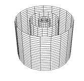
(a) $\theta_{0}=0$

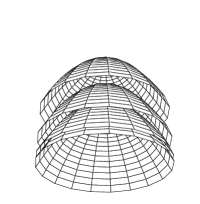
(b) $0<\theta_{0}<\pi$

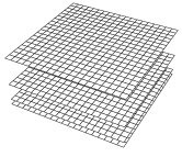
(c) $\theta_{0}=\pi$

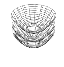
(d) $2\pi>\theta_{0}>\pi$

Figure 1. Foliation of $\theta_{0}=\text{constant}$ three-planes by conjugacy classes.

Consider first of all the case of $\theta_{0}=0$. Then we see that under the adjoint action (19),

$$g(0,w_{0},t_{0})\mapsto g\left(0,e^{i\theta}\,w_{0},t_{0}-\mathrm{Im}we^{-i\theta}\bar{w}_{0}\right)~{}.$$

We can distinguish two subcases:

• ($w_{0}=0$) In this case, $g(0,0,t_{0})$ belongs to the centre of $\EuScript{N}$ and hence is the only element in its conjugacy class $\EuScript{C}^{\prime}_{0,t_{0}}$. The centraliser of every such class is the group $\EuScript{N}$ itself.

• ($w_{0}\neq 0$) In this case, the conjugacy class is a cylinder (i.e., diffeomorphic to $\mathbb{R}\times S^{1}$) comprising those group elements of the form $g(0,w_{0}e^{i\theta},t)$, which shows that the conjugacy class is labelled by $|w_{0}|$. We denote this class by $\EuScript{C}_{0,|w_{0}|}$. The centraliser of a typical element $g(0,w_{0},0)$ in this class is the two-dimensional abelian subgroup $\EuScript{A}_{w_{0}}\subset\EuScript{N}$ whose elements are of the form $g(0,sw_{0},t)$, with $s$ and $t$ real numbers.

Figure 1(a) shows how these conjugacy classes foliate the three-plane in $\EuScript{N}$ corresponding to $\theta_{0}=0$.

Consider now $\theta_{0}=\pi$. In this case, under the adjoint action (19),

$$g(\pi,w_{0},t_{0})\mapsto g(\pi,2w+e^{i\theta}w_{0},t_{0})~{}.$$

This shows that the conjugacy class is a 2-plane labelled by $t_{0}$, denoted $\EuScript{C}_{\pi,t_{0}}$ and pictured in Figure 1(c). The centraliser of an element $g(\pi,w_{0},t_{0})$ in $\EuScript{C}_{\pi,t_{0}}$ is the two-parameter subgroup $\EuScript{S}_{w_{0}}\subset\EuScript{N}$ consisting of elements of the form

$$g(\theta,\tfrac{1}{2}(1-e^{i\theta})w_{0},t)~{}.$$

Topologically, $\EuScript{S}_{w_{0}}\cong\mathbb{R}\times S^{1}$; although as Lie groups it is not a product. Indeed, if we let $k(\theta,t):=g(\theta,\tfrac{1}{2}(1-e^{i\theta})w_{0},t)$, then we have

$$k(\theta_{1},t_{1})\,k(\theta_{2},t_{2})\\ =k\left(\theta_{1}+\theta_{2},t_{1}+t_{2}-\tfrac{1}{8}|w_{0}|^{2}\mathrm{Im}(1-e^{i\theta_{1}})(1-e^{i\theta_{2}})\right)~{}.$$

Finally we consider the case of general $\theta_{0}\neq 0,\pi$. The centraliser of an element $g(\theta_{0},w_{0},t_{0})$ with $\theta_{0}\neq 0,\pi$ is given by those elements of the form

$$g(\theta,(1-e^{i\theta})w_{0}(1-e^{i\theta_{0}})^{-1},t)~{},$$

which form a two-dimensional subgroup $\EuScript{S}_{z_{0}}\subset\EuScript{N}$ with $z_{0}:=w_{0}(1-e^{i\theta_{0}})^{-1}$. The conjugacy class, being diffeomorphic to $\EuScript{N}/\EuScript{S}_{z_{0}}$, is therefore two-dimensional. The conjugacy class is defined (having fixed $\theta_{0}$) by the value of the real-valued class function

$$F(\theta_{0},w_{0},t_{0}):=t_{0}\,\sin\tfrac{\theta_{0}}{2}+\tfrac{1}{4}|w_{0}|^{2}\,\cos\tfrac{\theta_{0}}{2}~{}.$$

Fixing a real number $k_{0}$ and $\theta_{0}\neq 0,\pi$, elements in the conjugacy class $\EuScript{C}_{\theta_{0},k_{0}}$ are of the form

$$g(\theta_{0},w,k_{0}-\tfrac{1}{4}|w|^{2}\cot\tfrac{\theta_{0}}{2})~{},$$

for $w\in\mathbb{C}$, which make up a paraboloid. We can distinguish two cases: $\theta_{0}\in(0,\pi)$ and $\theta_{0}\in(\pi,2\pi)$. They are illustrated in Figures 1(b) and 1(d), respectively.

Parenthetically, the function $F$ also distinguishes conjugacy classes when $\theta_{0}=\pi$ and even for $\theta_{0}=0$ when $|w_{0}|\neq 0$; whereas for $w_{0}=0$, it is the value of $t_{0}$ which now distinguishes the (pointlike) conjugacy classes.

3.5. Geometry of the conjugacy classes

Due to their interpretation as $\mathsf{D}$-branes, an important characteristic of a conjugacy class is its geometry. In particular we have seen above that in order to conclude that a conjugacy class may serve as Dirichlet boundary conditions for a WZW model, it was necessary to assume that it was non-degenerate relative to the bi-invariant metric. In this section we will elucidate the geometry of the conjugacy classes found above. We will see that the planar and paraboloidal conjugacy classes are flat and euclidean, whereas the cylindrical conjugacy class is degenerate. Therefore all but the cylindrical conjugacy classes can be understood as $\mathsf{D}$-branes, at least at our current level of understanding. Since the metric on $\EuScript{N}$ is bi-invariant, the calculation is simplified in that it is enough to determine the geometry at a point: all other points being related by the adjoint action of the group, which is an isometry. At the same time, left- or right-translating a conjugacy class does not alter its geometry.

As alluded to above, the bi-invariant metric on $\EuScript{N}$ is not unique (even up to scale): one can always add a term $bd\theta^{2}$ for $b\in\mathbb{R}$. Since, as we shall see, the conjugacy classes have constant $\theta$, the induced metric is impervious to the inclusion of this term.

3.5.1. The conjugacy classes $\EuScript{C}_{0,|w_{0}|}$

From the above considerations it is enough to work at a point, which we take to be the typical element $g_{0}:=g(0,w_{0},0)$. The conjugacy class is the set $\EuScript{C}=\{g(0,e^{i\theta}w_{0},t)\mid\theta,t\in\mathbb{R}\}$, and the centraliser is the subgroup $\EuScript{Z}=\{g(0,sw_{0},t)\mid s,t\in\mathbb{R}\}$. At the point $g_{0}$, the tangent space $T_{g_{0}}\EuScript{C}$ to the conjugacy class is spanned by the vectors $v_{1}=x_{0}\partial_{y}-y_{0}\partial_{x}$ and $v_{2}=\partial_{t}$, where $w_{0}=x_{0}+iy_{0}$. Computing their scalar product, we find that at the point $g(0,w_{0},0)$,

$$\langle v_{1},v_{1}\rangle=|w_{0}|^{2}~{},\langle v_{1},v_{2}\rangle=\langle v_{2},v_{2}\rangle=0~{}.$$

Therefore the metric is degenerate, and this means that this conjugacy class cannot be interpreted (at least straightforwardly) as a $\mathsf{D}$-brane. Notice that the tangent space $T_{g_{0}}\EuScript{Z}$ to the centraliser $\EuScript{Z}$ at the point $g_{0}$, is spanned by the vectors $u_{1}=x_{0}\partial_{x}+y_{0}\partial_{y}$ and $u_{2}=\partial_{t}$, which obey

$$\langle u_{1},u_{1}\rangle=|w_{0}|^{2}~{},\langle u_{1},u_{2}\rangle=\langle u_{2},u_{2}\rangle=0~{}.$$

As usual we find that at $g_{0}$, $T_{g_{0}}\EuScript{C}=\left(T_{g_{0}}\EuScript{Z}\right)^{\perp}$, but that in this case $T_{g_{0}}\EuScript{C}\cap T_{g_{0}}\EuScript{Z}\neq\{0\}$.

3.5.2. The conjugacy classes $\EuScript{C}_{\pi,t_{0}}$

Let us now fix the typical element $g_{0}:=g(\pi,0,t_{0})$. The conjugacy class of this element is the set $\EuScript{C}=\{g(\pi,w,t_{0})\mid w\in\mathbb{C}\}$ and the normaliser of the typical element is the subgroup $\EuScript{Z}=\{g(\pi+\theta,0,t_{0}+t)\mid\theta,t\in\mathbb{R}\}$. At the point $g_{0}$, the tangent space to the conjugacy class is spanned by the vectors $v_{1}=\partial_{x}$ and $v_{2}=\partial_{y}$, with metric

$$\langle v_{1},v_{1}\rangle=\langle v_{2},v_{2}\rangle=1~{},\langle v_{1},v_{2}\rangle=0~{}.$$

This metric is clearly non-degenerate and euclidean. It is also evidently flat. Therefore the resulting $\mathsf{D}$-brane is a flat euclidean $\mathsf{D}$-string. The tangent space to the centraliser subgroup at the point $g_{0}$ is spanned by $u_{1}=\partial_{\theta}$ and $u_{2}=\partial_{t}$, whose metric is

$$\langle u_{1},u_{2}\rangle=1~{},\langle u_{1},u_{1}\rangle=\langle u_{2},u_{2}\rangle=0~{},$$

which is non-degenerate and minkowskian. Again we have that $T_{g_{0}}\EuScript{C}=\left(T_{g_{0}}\EuScript{Z}\right)^{\perp}$, but now $T_{g_{0}}\EuScript{C}\cap T_{g_{0}}\EuScript{Z}=\{0\}$ , so that $T_{g_{0}}\EuScript{N}=T_{g_{0}}\EuScript{C}\oplus T_{g_{0}}\EuScript{Z}$.

3.5.3. The conjugacy classes $\EuScript{C}_{\theta_{0},k_{0}}$

We take $g_{0}:=g(\theta_{0},0,k_{0})$ as typical element. Its conjugacy class is the set $\EuScript{C}=\{g(\theta_{0},w,k_{0}-\tfrac{1}{4}|w|^{2}\cot\tfrac{\theta_{0}}{2})\mid w\in\mathbb{C}\}$, and its centraliser subgroup is $\EuScript{Z}=\{g(\theta,0,t)\mid\theta,t\in\mathbb{R}\}$. The tangent space to the conjugacy class at $g_{0}$ is spanned by the vectors $v_{1}=\partial_{x}$ and $v_{2}=\partial_{y}$, with metric

$$\langle v_{1},v_{1}\rangle=\langle v_{2},v_{2}\rangle=1~{},\langle v_{1},v_{2}\rangle=0~{}.$$

This metric is clearly non-degenerate, euclidean and flat. Therefore the resulting $\mathsf{D}$-brane is again a flat euclidean $\mathsf{D}$-string. The tangent space to the centraliser subgroup at the point $g_{0}$ is spanned by $u_{1}=\partial_{\theta}$ and $u_{2}=\partial_{t}$, whose metric is

$$\langle u_{1},u_{2}\rangle=1~{},\langle u_{1},u_{1}\rangle=\langle u_{2},u_{2}\rangle=0~{},$$

which is non-degenerate and minkowskian. Again we have that $T_{g_{0}}\EuScript{C}=\left(T_{g_{0}}\EuScript{Z}\right)^{\perp}$, and $T_{g_{0}}\EuScript{C}\cap T_{g_{0}}\EuScript{Z}=\{0\}$ , so that $T_{g_{0}}\EuScript{N}=T_{g_{0}}\EuScript{C}\oplus T_{g_{0}}\EuScript{Z}$.

3.6. Twisted conjugacy classes of the Nappi–Witten group

In this section we determine the twisted conjugacy classes in the Nappi–Witten group. As discussed above, they will all be translates of the twisted conjugacy classes corresponding to the automorphism $r$ defined in equation (18), which is a representative for the unique nontrivial (metric-preserving) outer automorphism in the Nappi–Witten group.

Thus let $C_{r}(\theta_{0},w_{0},t_{0})$ denote the twisted adjoint orbit of the element $g(\theta_{0},w_{0},t_{0})$:

$$C_{r}(\theta_{0},w_{0},t_{0})\\ :=\left\{g(\theta,w,t)g(\theta_{0},w_{0},t_{0})g(-\theta,-\bar{w},-t)^{-1}\mid(\theta,w,t)\in S^{1}\times\mathbb{C}\times\mathbb{R}\right\}~{}.$$

Using the group multiplication law (11), one can compute the twisted action. First of all notice that

$$g(-\theta,-\bar{w},-t)^{-1}=g(\theta,e^{i\theta}\bar{w},t)~{},$$

and therefore

$$g(\theta,w,t)g(\theta_{0},w_{0},t_{0})g(\theta,e^{i\theta}\bar{w},t)=g(\theta_{0}+2\theta,e^{i\theta}w_{0}+w+e^{i(2\theta+\theta_{0})}\bar{w},\\ \hfill t_{0}+2t-\tfrac{1}{2}\mathrm{Im}(we^{-i\theta}\bar{w}_{0})-\tfrac{1}{2}\mathrm{Im}((w+e^{i\theta}w_{0})e^{-i(\theta_{0}+2\theta)}w))~{}.$$ (20)

In order to determine the dimension of this orbit, we work out the isotropy of the point $(\theta_{0},w_{0},t_{0})$; that is, the subgroup of $\EuScript{N}$ whose twisted adjoint action leaves $g(\theta_{0},w_{0},t_{0})$ invariant. Equating the right-hand side of equation (20) with $g(\theta_{0},w_{0},t_{0})$ we find that $\theta=0$, $w=i\varrho e^{i\theta_{0}/2}$, and $t=\tfrac{1}{2}\varrho\mathrm{Re}(w_{0}e^{-i\theta_{0}/2})$, for some real parameter $\varrho$. In other words, the isotropy subgroup is one-dimensional and hence the twisted conjugacy classes are three-dimensional.

Since they have codimension one, it is possible to exhibit these twisted conjugacy classes as level sets of a function which is invariant under the twisted adjoint action. The infinitesimal generators of the twisted adjoint action are easy to work out and demanding that a function be invariant under their action gives a number of partial differential relations. The differential ring of functions satisfying these relations is generated by the function

$$G(\theta_{0},w_{0},t_{0})=\mathrm{Im}(w_{0}e^{-i\theta_{0}/2})~{}.$$

Hence each twisted conjugacy class is determined by a real number $k$, as the set of $g(\theta,w,t)$ for which

$$\mathrm{Im}(we^{-i\theta/2})=k~{}.$$ (21)

It may be worth remarking that the twisted conjugacy classes in this family are odd-dimensional. This is in sharp contrast with the case of conjugacy classes, which (at least in groups admitting bi-invariant metrics) always have even dimension. This follows because conjugacy classes are the image under the exponential map of the adjoint orbits, which are diffeomorphic to the co-adjoint orbits which are symplectic manifolds relative to the natural Kirillov–Kostant–Souriau symplectic structure, and hence are even-dimensional.

3.7. Geometry of the twisted conjugacy classes

The induced metric on the twisted conjugacy classes can be worked out as follows. Let us introduce polar coordinates $(r,\phi)$ related to $w$ in the usual way: $w=re^{i\phi}$. Let us assume that $k\neq 0$. We can then eliminate the radial coordinate $r$ using equation (21):

$$r=k\csc(\phi-\tfrac{1}{2}\theta)~{}.$$

It is convenient to eliminate $\phi$ in terms of the real variable $z=\cot(\phi-\tfrac{1}{2}\theta)$. In terms of the coordinates $(z,\theta,t)$ parametrising the twisted conjugacy class, the metric (17) becomes

$$ds^{2}=k^{2}dz^{2}+2d\theta\left(dt-\tfrac{1}{8}k^{2}(1+z^{2})d\theta\right)~{},$$ (22)

which is clearly non-degenerate and of lorentzian signature. Therefore twisted conjugacy classes define $\mathsf{D}$-membranes. Unlike the euclidean $\mathsf{D}$-strings associated to the conjugacy classes, these membranes are not flat and, since in three dimensions, Ricci-flatness implies flatness, they are not Ricci-flat either. To see this let us simply notice that the riemannian connection is given by

$$\nabla_{\theta}\partial_{\theta}=\tfrac{1}{4}z\partial_{z}\qquad\text{and}\qquad\nabla_{\theta}\partial_{z}=\nabla_{z}\partial_{\theta}=-\tfrac{1}{4}k^{2}z\partial_{t}~{},$$

whence the riemannian curvature tensor has components

$$R_{z\theta\theta}{}^{z}=-\tfrac{1}{4}\qquad\text{and}\qquad R_{z\theta z}{}^{t}=\tfrac{1}{4}k^{2}~{}.$$

Notice that the Ricci tensor has non-vanishing components $R_{\theta\theta}=\tfrac{1}{4}$, but that the scalar curvature does vanish.

Let us remark that the membrane admits parallel spinors. In fact, it is an example of an indecomposable Ricci-null lorentzian manifold (see for example [3]) with holonomy group isomorphic to $\mathbb{R}\subset\mathrm{SO}(2,1)$. In fact the membrane metric conforms to the metric given by equation (17) in [3], which is the most general three-dimensional lorentzian metric admitting parallel spinors.

The same conclusion can be reached for $k=0$; although the details are different. In this case, we do not eliminate $r$, but rather notice that in this case $\phi=2\theta$, whence in terms of the real coordinates $(r,\theta,t)$, the induced metric on the membrane is given by

$$ds^{2}=dr^{2}+2d\theta\left(dt-\tfrac{3}{8}r^{2}d\theta\right)~{},$$ (23)

which again describes an indecomposable three-dimensional lorentzian manifold admitting parallel spinors.

Let us remark that the induced metric on the twisted conjugacy classes is affected by including the term $bd\theta^{2}$ coming from the ambiguity in the invariant scalar product $\mathfrak{n}$; but this does not change qualitatively the geometry of the brane. One still obtains indecomposable three-dimensional lorentzian manifolds admitting parallel spinors.

In summary, we see that the Nappi–Witten group admits curved membranes admitting parallel spinors, flat euclidean strings and instantons among its $\mathsf{D}$-branes.

4. Conclusions

In this paper we have re-examined the possible boundary conditions in a WZW model which are compatible with conformal invariance. We have shown (following [6]) how to relate gluing conditions on the chiral currents to geometric boundary conditions of the group valued fields in the classical description of the WZW model. We have seen that a natural solution to the consistency conditions are given by (twisted) conjugacy classes: the orbits of group elements under the adjoint action twisted by an automorphism. When the automorphism is trivial, the resulting orbits are conjugacy classes, and when it is inner the orbits are shifted conjugacy classes. More generally, two automorphisms whose “difference” is an inner automorphism give rise to orbits which are shifted relative to each other. This suggests that one should use the group of (metric-preserving) outer automorphisms as a sort of classifying group for boundary conditions.

It is important to keep in mind that not all boundary conditions are given by (twisted) conjugacy classes, as shown in [8, 7, 6].

We have then illustrated these results in the case of the Nappi–Witten group. In that case the group of (metric-preserving) outer automorphisms has order 2, and hence there are two distinct families of possible boundary conditions. One family gives rise to (shifted) conjugacy classes. Studying their geometry, we have seen that these classes consist of flat euclidean $\mathsf{D}$-strings and $\mathsf{D}$-instantons. The other family of boundary conditions gives rise to $\mathsf{D}$-membranes which are not flat: they are indecomposable lorentzian manifolds admitting parallel spinors.

References

- [1] AY Alekseev and V Schomerus, D-branes in the WZW model, Phys. Rev. D60 (1999), 061901, hep-th/9812193.
- [2] G Felder, J Fröhlich, J Fuchs, and C Schweigert, The geometry of WZW branes, hep-th/9909030.
- [3] JM Figueroa-O’Farrill, Breaking the -waves, hep-th/9904124.
- [4] JM Figueroa-O’Farrill and S Stanciu, Nonreductive WZW models and their CFTs, Nuc. Phys. B458 (1996), 137–164, hep-th/9506151.
- [5] C Nappi and E Witten, A WZW model based on a non-semi-simple group, Phys. Rev. Lett. 71 (1993), 3751–3753, hep-th/9310112.
- [6] S Stanciu, D-branes in group manifolds, hep-th/9909163.
- [7] by same author, D-branes in an background, J. High Energy Phys. 09 (1999), 028, hep-th/9901122.
- [8] S Stanciu and A A Tseytlin, D-branes in curved spacetime: the Nappi–Witten background, J. High Energy Phys. 06 (1998), 010, hep-th/9805006.