Interacting strings on $AdS_{3}$

Gastón Giribet and Carmen A. Núñez

Instituto de Astronomía y Física del Espacio

IAFE - CONICET

C.C. 67 - Suc. 28, 1428 Buenos Aires, Argentina

We consider string theory on $AdS_{3}$ in terms of the Wakimoto free field representation. The scattering amplitudes for N unitary tachyons are analysed in the factorization limit and the poles corresponding to the mass-shell conditions for physical states are extracted. The vertex operators for excited levels are obtained from the residues and their properties are examined. Negative norm states are found at the second mass level.

PACS: 11.25.-w

Keywords: string theory, Anti de Sitter space

1 Introduction

String theory on three dimensional Anti-de Sitter spacetime has been extensively studied in the past [1, 2, 3, 4, 5] as a toy model to investigate the consistency of string propagation on background fields. This is an interesting example since it provides a realization of the Kac-Moody algebra of $SL(2,R)$, and is thus an exactly solvable model. Renewed interest in the subject originated more recently after Maldacena’s conjecture [6] which suggests a duality between string theory formulated on $AdS_{D}$ and a conformal field theory living on the $(D-1)$ dimensional boundary of $AdS$ spacetime. The case $D=3$ has attracted special attention since the conjecture could be worked out in full detail and explicitly verified [7, 8, 9] in this model.

However the structure of two dimensional non linear sigma models on non compact spaces presents several problems. The quantum mechanical propagation of strings on $AdS_{3}$ is not consistent. The Virasoro constraints are not sufficient to decouple the negative norm states of the spectrum. Several proposals have been advanced in the literature [2, 3, 4, 5, 10, 11] to render the theory unitary, but there is no general agreement yet. A no ghost theorem has been proved for strings on $AdS_{3}$ at free level [12]. Unitarity is achieved by keeping only states with quantum numbers $j$ bounded by the level of the algebra $k$ ($-1<j<k/2-1$). But this is not enough: a consistent string theory should provide a mechanism to avoid the negative norm states at the interacting level, similarly as in flat spacetime, i.e. non physical states must decouple in physical processes. This implies that fusion rules should close among ghost-free representations. Moreover, while the spectrum of the compact current algebras can be truncated to the unitary representations without spoiling modular invariance it is not clear that this can be done in the non-compact case.

Furthermore it has been claimed that the $AdS/CFT$ correspondence suggests a relationship between the conformal weights of the fields in the boundary conformal field theory, $h$ and the quantum number $j$ labeling the states of string theory in $AdS_{3}$ [7]. This assumption would lead to an inconsistency for the ground state tachyon belonging to the unitary principal continuous representation $j\in-\frac{1}{2}+i\lambda$ [8] since consistency of the spacetime $CFT$ requires $h$ to be real and thus it would darken the range of validity of the conjecture. It is possible that the boundary $CFT$ gives a more comprehensive description of the fundamental degrees of freedom of M-theory, but it is important to fill in the details of the $AdS/CFT$ duality map in order to completly understand the correspondence.

In standard perturbative string theory particles of various masses and spins are exchanged in the different channels of a scattering amplitude. They appear as singularities in the appropriate square momentum variable. One can think of obtaining all the physical states of the spectrum of strings on $AdS_{3}$ and study their properties by analysing the scattering amplitudes of the lowest energy particles in the theory. The purpose of this paper is to address this question in the bosonic theory, starting from the correlation functions of an arbitrary number of tachyons. Unlike string theory in Minkowski spacetime, strings propagating on the non-compact $SL(2,R)$ group manifold have an infinite degeneracy of states at a given mass level. Nevertheless the scattering amplitudes exhibit several similarities with the flat case. Singularities occur when the points where some of the external vertex operators are attached coincide. The poles correspond to the mass shell conditions for the intermediate states and the residues reproduce the scattering amplitudes of the remaining tachyons with the exchanged states. From this expression it is possible to extract the vertex operator corresponding to the intermediate states, at arbitrary excited level.

In order to have a clear spacetime interpretation we consider the universal covering of $SL(2,R)$ which is topologically $R^{2}\times R$, because time is periodic on the group itself which is topologically $R^{2}\times S^{1}$. Moreover we work in the Wakimoto representation of the theory in terms of free fields. In this formalism the string coupling constant depends on one of the spacetime coordinates. Therefore our results are reliable near the boundary of spacetime where the theory becomes weakly coupled. However since $AdS$ is a constant curvature spacetime it is reasonable to assume that the spectrum of states of the theory does not depend on the region of spacetime where it is located. In principle one should be able to find all the possible states of the spectrum in this way (or at least all those that couple to tachyons).

Conformal invariance imposes constraints on the vertex operators which are automatically satisfied when this formalism is developed in flat spacetime on arbitrary Riemann surfaces [13]. In the case under consideration we have explicitly verified up to the second excited level that the vertex operators obtained from factorization are automatically $CFT$ primaries.

This paper is organized as follows. In section 2 we review string theory on $AdS_{3}$. We summarize the $SL(2,R)$ WZW model in terms of the Wakimoto free field representation and discuss the spectrum of string theory in this background. In section 3 we present the tachyon vertex operator and the formalism that has been developed in the literature to compute correlation functions, following closely [14]. We perform the factorization of the $N$-tachyon scattering amplitude and obtain the poles corresponding to the mass-shell condition for physical states. By analysing the residue we reobtain the vertex operator for the intermediate tachyon state. In section 4 we study the higher order poles. We find the vertex operators for the first and second excited levels and examine their properties. At the first mass level all the states produced are unitary whereas negative norm states are found at the second mass level even though the original amplitude involves only unitary external tachyons. Finally the conclusions in section 5 contain a discussion of the implications of this result. As a by-product the general form of the vertex operator for an arbitrary excited level which can be expected from this particular factorization process is given.

2 Strings on $AdS_{3}$

In this section we review some basic facts of string theory on $AdS_{3}$ in order to introduce notation.

The $SL(2,R)$ Wess-Zumino-Witten model is given, in the Gauss parametrization, by

$$S=k\int d^{2}z[\partial\phi\bar{\partial}\phi+\bar{\partial}\gamma\partial\bar{\gamma}e^{2\phi}]$$ (1)

This action describes strings propagating in three dimensional Anti-de Sitter space with curvature $-\frac{2}{k}$, metric

$$ds^{2}=kd\phi^{2}+ke^{2\phi}d\gamma d\bar{\gamma}$$ (2)

and background antisymmetric field

$$B=ke^{2\phi}d\gamma\wedge d\bar{\gamma}$$ (3)

The boundary of $AdS_{3}$ is located at $\phi\rightarrow\infty$. Near this region quantum effects can be treated perturbatively, the exponent in the last term in (1) is renormalized and a linear dilaton in $\phi$ is generated. Adding auxiliary fields $(\beta,\bar{\beta})$ and rescaling, the action becomes [15]

$$S=\frac{1}{4\pi}\int d^{2}z[\partial\phi\bar{\partial}\phi-\frac{2}{\alpha_{+}}R\phi+\beta\bar{\partial}\gamma+\bar{\beta}\partial\bar{\gamma}-\beta\bar{\beta}e^{-\frac{2}{\alpha_{+}}\phi}]$$ (4)

where $\alpha_{+}=\sqrt{2(k-2)}$. This action can be trusted for large values of $\phi$.

This theory has a non-compact symmetry generated by currents $J^{a}(z)$ and $\bar{J}^{a}(\bar{z})$, $a=1,2,3$. In the following we discuss the holomorphic part of the theory because the same considerations apply to the antiholomorphic part.

Expanding in a Laurent series,

$$J^{a}(z)=\sum_{n=-\infty}^{\infty}J_{n}^{a}z^{-n-1}$$ (5)

the coefficients $J_{n}^{a}$ satisfy a Kac-Moody algebra given by

$$[J^{a}_{n},J^{b}_{m}]=if^{ab}_{~{}~{}~{}c}J^{c}_{m+n}-{\frac{k}{2}}g^{ab}n\delta_{n+m,0}$$ (6)

where the structure constants can be chosen as $f^{abc}=\epsilon^{abc}$ and the Cartan Killing metric is of the form $g^{ab}=diag(+1,+1,-1)$.

It is useful to introduce the complex basis $(J^{\pm},J^{3})$ where

$$J^{\pm}=J^{1}\pm iJ^{2}\quad,\quad(J^{\pm})^{{\dagger}}=J^{\mp}$$ (7)

and the Kac Moody algebra takes the form

$$[J^{3}_{m},J^{3}_{n}]=-{\frac{k}{2}}m\delta_{m+n,0}$$ (8)

$$[J^{3}_{m},J^{\pm}_{n}]=\pm J^{\pm}_{m+n}$$ (9)

$$[J^{+}_{m},J^{-}_{n}]=-2J^{3}_{m+n}+km\delta_{m+n,0}$$ (10)

This $SL(2,R)$ current algebra can be expressed in terms of the fields $(\phi,\beta,\gamma)$ using the Wakimoto representation [16]

$$J^{+}(z) = \beta(z)$$ (11)

$$J^{3}(z) = -\beta(z)\gamma(z)-\frac{\alpha_{+}}{2}\partial\phi(z)$$

$$J^{-}(z) = \beta(z)\gamma^{2}(z)+\alpha_{+}\gamma(z)\partial\phi(z)+k\partial\gamma(z)$$

Indeed, considering the free field propagators

$$\left\langle\phi(z)\phi(w)\right\rangle=-\log(z-w)$$ (12)

$$\left\langle\gamma(z)\beta(w)\right\rangle=-\frac{1}{(z-w)}$$ (13)

it is easy to verify that the OPEs of these currents realize a $SL(2,R)$ level $k$ Kac-Moody algebra, namely

$$J^{+}(z)J^{-}(w) = \frac{k}{(z-w)^{2}}-\frac{2}{(z-w)}J^{3}(w)+...$$

$$J^{3}(z)J^{\pm}(w) = \pm\frac{1}{(z-w)}J^{\pm}(w)+...$$

$$J^{3}(z)J^{3}(w) = \frac{-k/2}{(z-w)^{2}}+...$$

The Sugawara construction leads to the following energy-momentum tensor

$$T(z)=\beta\partial\gamma-\frac{1}{2}(\partial\phi)^{2}-\frac{1}{\alpha_{+}}\partial^{2}\phi$$ (14)

and hence the central charge of the theory is

$$c=\frac{3k}{(k-2)}$$ (15)

This implies that $k=52/23$ when the theory is formulated on $AdS_{3}$. In general there could be an internal compact space ${\cal N}$ ($i.e.$ the theory lives on $AdS_{3}\times{\cal N}$), and in this case $k>52/23$.

The spectrum of the theory can be obtained analysing the $SL(2,R)$ Kac-Moody primary states. They are labeled by two quantum numbers $\left|j,m\right\rangle$, where

$$\Delta_{o}\left|j,m\right\rangle = j(j+1)\left|j,m\right\rangle$$ (16)

$$J_{o}^{3}\left|j,m\right\rangle = m\left|j,m\right\rangle$$

and $\Delta_{o}=:-\frac{1}{2}(J_{o}^{+}J_{o}^{-}+J_{o}^{-}J_{o}^{+})+J_{o}^{3}J_{o}^{3}:$ is the Casimir (the subindices refer to the zero-modes of the currents). The ground states $\left|j,m\right\rangle$ satisfy

$$J_{n}^{a}\left|j,m\right\rangle = 0,\quad n>0$$ (17)

The complete representation can be constructed by acting with the zero-modes of the currents, namely

$$J_{o}^{+}\left|j,m\right\rangle = (j-m)\left|j,m+1\right\rangle$$ (18)

$$J_{o}^{-}\left|j,m\right\rangle = (-j-m)\left|j,m-1\right\rangle$$

It is possible to restrict the group representations by requiring hermiticity and unitarity. Hermiticity implies that $J_{o}^{3}$ and $\Delta_{o}$ have a real spectrum, namely $\{m\in R$ , $j\in R\}$ or $\{m\in R$ , $j\in-\frac{1}{2}+iR\}$. Notice that in order to have a clear spacetime interpretation we work on the universal covering of $SL(2,R)$. On the group itself $m$ is quantized and restricted to be integer. Unitarity at the base requires [3, 5]

$$m(m\pm 1)-j(j+1)\geq 0$$

The unitary representations of the universal covering of $SL(2,R)$ are classified as follows: $a)$ the principal continuous series with $j={\frac{1}{2}}\pm i\lambda$, $\lambda\in R$ and $m\in R$; $b)$ the discrete series, $D_{j}^{\pm}$ with highest and lowest weight states having $j=\pm m$, $m\in R$; $c)$ the exceptional representation with $-{\frac{1}{2}}\leq j<0,m\in R$ and the trivial representation with $j=m=0$.

The excited states are constructed by acting with $J_{-n}^{a}$, $n>0$ on the ground state representation.

The string states must satisfy the Virasoro constraints $L_{m}\left|\Psi\right\rangle=0$, $m>0$ and $L_{o}\left|\Psi\right\rangle=\left|\Psi\right\rangle$. The last one implies

$$-\frac{j(j+1)}{(k-2)}+L=1$$ (19)

at excited level $L$. Notice that this expression is invariant under $j\rightarrow-j-1$ and therefore one can consider only states with $j>-{\frac{1}{2}}$ or $j<-{\frac{1}{2}}$.

Taking into account that the Casimir plays the role of mass squared operator [5], the mass spectrum of the theory is

$$M^{2}=\frac{(L-1)}{2}\alpha_{+}^{2}$$ (20)

Therefore, the ground state of the bosonic theory is a tachyon, the first excited level contains massless states and there is an infinite tower of massive states.

Notice that the on-shell tachyon of the theory living on $AdS_{3}$ has $j=-{\frac{1}{2}}\pm{\frac{i}{\sqrt{92}}}$ and thus belongs to the unitary principal continuous series. If there is an internal compact space ${\cal N}$, eq. (19) becomes

$$-{\frac{j(j+1)}{{k-2}}}+L+\Delta=1$$ (21)

where $\Delta$ is the contribution of the internal part.

3 Interactions

In this section we discuss string interactions on $AdS_{3}$. The aim is to read the states of the spectrum and their vertex operators from the residues of the poles in the combinations of quantum numbers corresponding to the masses of the intermediate states.

As a starting point for the computation, the amplitude for the scattering of physical particles has to be constructed. This procedure requires, as initial data, the vertex operators of the external particles to be scattered. The natural objects to start with are the lowest energy states, i.e. tachyons. The tachyon vertex operator was originally constructed in reference [17] by looking at the conformal dimensions and OPE with the currents of fields in the $SL(2,R)_{k}$ $WZW$ theory, and it is given by

$$V_{T}(j,m)=:\gamma^{j-m}(z)\bar{\gamma}^{j-\bar{m}}(\bar{z})e^{\frac{2j}{\alpha_{+}}\phi(z,\bar{z})}:$$ (22)

where $m-\bar{m}\in Z$ is necessary for single valuedness. This vertex operator should be supplemented with an appropriate internal part if the theory is formulated on $AdS_{3}\times{\cal N}$.

Note that this is a different representation than the one introduced by Teschner [18]. The operator (22) corresponds to the leading large $\phi$ part of Teschner’s representation, i.e. it is suitable to work in the near boundary limit. The large $\phi$ approximation leads to incomplete results for correlation functions [8, 9]. However it is sufficient for our purposes of extracting the short distance singularities of the scattering amplitudes signaling the on-mass-shell states of the theory. Indeed, it is reasonable to expect that the spectrum of the theory will not depend on the region of spacetime where the string is located (unless there were singularities).

We now review the formalism to construct the $N$-point function of tachyons. This approach was developed in [14] and it is well suited to our purposes. The starting point is the following scattering amplitude

$$A_{m_{1}...m_{N}}^{j_{1}...j_{N}}=Vol[SL(2,C)]^{-1}\left\langle\mathop{\displaystyle\prod}_{i=1}^{N}\displaystyle\int d^{2}z_{i}V_{T}(j_{i},m_{i})\right\rangle$$ (23)

where the average is performed with respect to the action (4). The antiholomorphic dependence $j_{i}=\bar{j}_{i}$ and $m_{i}=\bar{m}_{i}$ is implicit in this notation.

The integration over the zero-modes of the fields leads to a charge conservation condition for non-vanishing amplitudes which can be achieved through the inclusion of screening operators [19]. These operators were constructed in reference [17] and can be represented as

$${\cal S}=\int d^{2}w\beta(w)\bar{\beta}(\bar{w})e^{-\frac{2}{\alpha_{+}}\phi(w,\bar{w})}$$ (24)

Therefore the amplitude (23) takes the form

$$A_{m_{1}...m_{N}}^{j_{1}...j_{N}}=Vol^{-1}[SL(2,C)]\left\langle\mathop{\displaystyle\prod}_{i=1}^{N}\displaystyle\int d^{2}z_{i}V_{T}(j_{i},m_{i})\left(\int d^{2}w\beta\bar{\beta}e^{-\frac{2}{\alpha_{+}}\phi}\right)^{s}\right\rangle$$ (25)

where the Gauss-Bonnet theorem implies, at the tree level

$$s=\sum_{i=1}^{N}j_{i}+1$$ (26)

Note that if the tachyons belong to the principal continuous series $s$ will not be in general a positive integer. However, the prescription developed in [15] for the equivalent situation in Liouville theory, consists in assuming that the number of screenings is a positive integer and the correlators are evaluated by analytic continuation.

The integration over the zero-modes of the $(\beta,\gamma)$ system leads to the following condition

$$(number~{}of~{}\beta~{}fields)-(number~{}of~{}\gamma~{}fields)=1$$ (27)

for non-vanishing correlation functions. In the case under consideration, this equation is

$$s=\sum_{i=1}^{N}(j_{i}-m_{i})+1$$ (28)

From (26) and (28) the following conservation law is obtained

$$\sum_{i=1}^{N}m_{i}=0$$ (29)

Therefore the $N$-point function for tachyons can be written as

$$A_{m_{1}...m_{N}}^{j_{1}...j_{N}} = \frac{1}{Vol[SL(2,C)]}\displaystyle\int\prod_{i=1}^{N}d^{2}z_{i}\mathop{\displaystyle\prod}_{n=1}^{s}\displaystyle\int d^{2}w_{n}\left\langle\prod_{i=1}^{N}\gamma_{(z_{i})}^{j_{i}-m_{i}}\prod_{n=1}^{s}\beta(w_{n})\right\rangle\times$$

$$\ \ \ \times\left\langle\prod_{i=1}^{N}\bar{\gamma}_{(\bar{z}_{i})}^{j_{i}-m_{i}}\prod_{n=1}^{s}\bar{\beta}(\bar{w}_{n})\right\rangle\times\left\langle\prod_{i=1}^{N}e^{\frac{2}{\alpha_{+}}j_{i}\phi(z_{i},\bar{z}_{i})}\prod_{n=1}^{s}e^{-\frac{2}{\alpha_{+}}\phi(w_{n},\bar{w}_{n})}\right\rangle$$

Here $(z_{i},\bar{z}_{i})$ and $(w_{n},\bar{w}_{n})$ are the world-sheet coordinates where the tachyonic and the screening vertex operators respectively are inserted.

Using the propagators (12) and (13) this amplitude becomes

$$A_{m_{1}...m_{N}}^{j_{1}...j_{N}} \sim \displaystyle\int\mathop{\displaystyle\prod}_{i=1}^{N}d^{2}z_{i}\mathop{\displaystyle\prod}_{r=1}^{s}d^{2}w_{n}C(z_{i},w_{n})\bar{C}(\bar{z}_{i},\bar{w}_{n})\prod_{i<k}\left|z_{i}-z_{k}\right|^{-8j_{i}j_{k}/\alpha_{+}^{2}}\times$$ (30)

$$\ \ \times\prod_{i,n}\left|z_{i}-w_{n}\right|^{8j_{i}/\alpha_{+}^{2}}\times\prod_{n<m}\left|w_{n}-w_{m}\right|^{-8/\alpha_{+}^{2}}$$

where $C(z_{i},w_{n})$ and $\bar{C}(\bar{z}_{i},\bar{w}_{n})$ stand for the contribution of the $(\beta,\gamma)$ correlators (see eq.(34) below).

The corresponding expression in stardard string perturbation theory in Minkowski spacetime exhibits some aspects of tree level unitarity. It has poles for on-mass-shell states and the residue of each pole factorizes as the product of tree amplitudes for subprocesses $1,2,3,...M,J\rightarrow J,(M+1),...N$ as depicted in Fig.1.

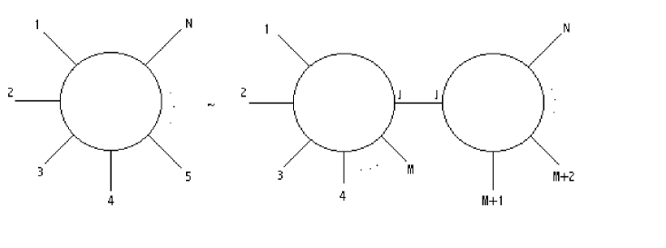
Figure 1: Factorizacion of scattering amplitude

The physical singularities of the amplitude (30) can be extracted by considering the region of integration where a subset of the $N$ tachyons collide to the same point on the world-sheet. Unitarity requires also that the intermediate state $J$ has non-negative norm. We would like to check whether these properties hold in string theory on $AdS_{3}$ when two external vertex operators coincide. In this case, the factorization should take the form

$$A_{m_{1}...m_{N}}^{j_{1}...j_{N}}\sim\frac{\left\langle V_{T(j_{1},m_{1})}V_{T(j_{2},m_{2})}\tilde{V}_{T(j,m)}\right\rangle\times\left\langle V_{T(j,m)}V_{T(j_{3},m_{3})}V_{T(j_{4},m_{4})}...V_{T(j_{N},m_{N})}\right\rangle}{-\frac{2j(j+1)}{\alpha_{+}^{2}}+L-1}$$ (31)

where the conjugate vertex operator $\tilde{V}_{(j,m)}$ is $V_{(-j-1,-m)}$ [17], $(j,m)$ are the quantum numbers of the intermediate state and $L\in Z$.

The conditions for non-vanishing residue in this expression are the following

$$s_{1}=j_{1}+j_{2}-j\qquad;\qquad m=m_{1}+m_{2}$$ (32)

$$s_{2}=\mathop{\displaystyle\sum}_{i=3}^{N}j_{i}+j+1\qquad;\qquad m+\mathop{\displaystyle\sum}_{i=3}^{N}m_{i}=0$$ (33)

where $s_{1}$ and $s_{2}$ are the number of screening operators in the $3$-point and $(N-1)$-point functions respectively.

Let us consider the particular case $z_{2}\rightarrow z_{1}$ and take the $s_{1}$ contours to encircle $z_{1}$ and $z_{2}$ [19]. To isolate the singularities corresponding to the intermediate channels perform the change of variables: $z_{1}-z_{2}=\varepsilon,$ $z_{1}-v_{n}=\varepsilon y_{n},$ $v_{n}-z_{2}=\varepsilon(1-y_{n})$, where we have renamed as $v_{n}$ the insertion points of the $s_{1}$ contours.

In order to extract the explicit $\varepsilon$ dependence of the amplitude it is convenient to write the functions $C(z_{i},v_{n},w_{m})$ and $\bar{C}(\bar{z}_{i},\bar{v}_{n},\bar{w}_{m})$ as

$$C(z_{i},v_{n},w_{m}) = \left\langle\gamma^{j_{1}-m_{1}}(z_{1})\gamma^{j_{2}-m_{2}}(z_{2})\mathop{\displaystyle\prod}_{i=3}^{N}\gamma^{j_{i}-m_{i}}(z_{i})\mathop{\displaystyle\prod}_{n=1}^{s_{1}}\beta(v_{n})\mathop{\displaystyle\prod}_{m=1}^{s_{2}}\beta(w_{m})\right\rangle$$

$$\sim \mathop{\displaystyle\sum}_{Perm(v_{n})}\mathop{\displaystyle\sum}_{k=0}^{s_{1}}\frac{(j_{1}-m_{1})(j_{1}-m_{1}-1)...(j_{1}-m_{1}-k+1)}{(z_{1}-v_{1})(z_{1}-v_{2})...(z_{1}-v_{k})}\times$$

$$~{}~{}~{}~{}~{}~{}~{}~{}~{}~{}~{}~{}~{}\times\frac{(j_{2}-m_{2})(j_{2}-m_{2}-1)..(j_{2}-m_{2}-s_{1}+k+1)}{(z_{2}-v_{k+1})...(z_{2}-v_{s_{1}})}\times$$

$$\ \times\left\langle\gamma^{j_{1}-m_{1}-k}(z_{1})\gamma^{j_{2}-m_{2}-s_{1}+k}(z_{2})\mathop{\displaystyle\prod}_{i=3}^{N}\gamma^{j_{i}-m_{i}}(z_{i})\mathop{\displaystyle\prod}_{m=1}^{s_{2}}\beta(w_{m})\right\rangle+$$

$$\ \ +\mathop{\displaystyle\sum}_{Perm(v_{n})}\mathop{\displaystyle\sum}_{k=0}^{s_{1}-1}\frac{(j_{1}-m_{1})(j_{1}-m_{1}-1)...(j_{1}-m_{1}-k+1)}{(z_{1}-v_{1})(z_{1}-v_{2})...(z_{1}-v_{k})}\times$$

$$\ \ \times\frac{(j_{2}-m_{2})(j_{2}-m_{2}-1)..(j_{2}-m_{2}-s_{1}+k+2)}{(z_{2}-v_{k+1})...(z_{2}-v_{s_{1}-1})}\mathop{\displaystyle\sum}_{i=3}^{N}\frac{j_{i}-m_{i}}{z_{i}-v_{s_{1}}}\times$$

$$\ \ \times\left\langle\gamma^{j_{1}-m_{1}-k}(z_{1})\gamma^{j_{2}-m_{2}-s_{1}+k+1}(z_{2})\mathop{\displaystyle\prod}_{l\neq i}\gamma^{j_{l}-m_{l}}(z_{l})\gamma^{j_{i}-m_{i}-1}(z_{i})\mathop{\displaystyle\prod}_{m=1}^{s_{2}}\beta(w_{m})\right\rangle+...$$

(34)

and similarly for $\bar{C}(\bar{z}_{i},\bar{v}_{n},\bar{w}_{n})$. The sign $\sim$ stands for an irrelevant phase. The products $(j_{1}-m_{1})(j_{1}-m_{1}-1)...(j_{1}-m_{1}-k+1)$ have to be understood as not contributing for $k=0$ (similarly $(j_{2}-m_{2})...(j_{2}-m_{2}-s_{1}+k+1)$ for $k=s_{1}$). The dots stand for lower order contractions between the fields inserted at $z_{1}$ and $z_{2}$ and the $s_{1}$ screening operators. Note that these functions can be written as a power series in $\varepsilon$ after performing the change of variables and extracting the leading $\varepsilon^{-s_{1}}$ divergence.

The amplitude becomes then formally

$$A_{m_{1}...m_{N}}^{j_{1}...j_{N}} \sim \displaystyle\int d^{2}\varepsilon\left|\varepsilon\right|^{2s_{1}-[8j_{1}j_{2}-8s_{1}j_{1}-8j_{2}s_{1}+4s_{1}(s_{1}-1)]/\alpha_{+}^{2}-2s_{1}}\times$$

$$\times\displaystyle\int d^{2}z_{1}\prod_{i=3}^{N}\displaystyle\int d^{2}z_{i}\mathop{\displaystyle\prod}_{n=1}^{s_{2}}d^{2}w_{n}\mathop{\displaystyle\prod}_{r=1}^{s_{1}}\displaystyle\int d^{2}y_{r}\left|\Phi(\varepsilon,z_{1},z_{i},y_{r},w_{n})\Psi(z_{i},w_{n})\right|^{2}$$

The first term in the exponent of $\left|\varepsilon\right|$ comes from the change of variables in the insertion points of the $s_{1}$ screening operators whereas the last term cancelling it arises in the $\beta-\gamma$ system, eq. (34). The other terms in the exponent originate in the contractions of the exponentials. The function $\Phi$ is a regular function in the limit $\varepsilon\rightarrow 0$. It is convenient to write separately the contribution to $\Phi$ from the exponentials ($E$) and from the $\beta-\gamma$ system ($C$), i.e. $\Phi=E\times|C|^{2}$, where

$$E(\varepsilon,z_{1},z_{i},y_{r},w_{n})=\prod_{r=1}^{s_{1}} |y_{r}|^{8j_{1}/\alpha_{+}^{2}}|1-y_{r}|^{8j_{2}/\alpha_{+}^{2}}\prod_{r<t}|y_{r}-y_{t}|^{-8/\alpha_{+}^{2}}$$

$$\prod_{i=3}^{N} |z_{1}-z_{i}|^{-8j_{1}j_{i}/\alpha_{+}^{2}}|z_{1}-\varepsilon-z_{i}|^{-8j_{2}j_{i}/\alpha_{+}^{2}}$$

$$\prod_{m=1}^{s_{2}} |z_{1}-w_{m}|^{8j_{1}/\alpha_{+}^{2}}|z_{1}-\varepsilon-w_{m}|^{8j_{2}/\alpha_{+}^{2}}$$

$$\prod_{i=3}^{N}\prod_{r=1}^{s_{1}} |z_{i}-z_{1}+\varepsilon y_{r}|^{8j_{i}/\alpha_{+}^{2}}\prod_{r=1}^{s_{1}}\prod_{m=1}^{s_{2}}|z_{1}-\varepsilon y_{r}-w_{m}|^{-8/\alpha_{+}^{2}}$$

and

$$C(\varepsilon,z_{1},z_{i},y_{r},w_{n})\sim\mathop{\displaystyle\sum}_{Perm(y_{n})}\mathop{\displaystyle\sum}_{k=0}^{s_{1}}\frac{(j_{1}-m_{1})(j_{1}-m_{1}-1)...(j_{1}-m_{1}-k+1)}{y_{1}y_{2}...y_{k}}\times$$

$$~{}~{}~{}~{}~{}~{}\times\frac{(j_{2}-m_{2})(j_{2}-m_{2}-1)...(j_{2}-m_{2}-s_{1}+k+1)}{(1-y_{k+1})(1-y_{k+2})...(1-y_{s_{1}})}\times$$

$$\sum_{Perm(w_{m})}{\large\{}{\large[}{-\frac{(j_{1}-m_{1}-k)}{z_{1}-w_{1}}}-\frac{(j_{2}-m_{2}-s_{1}+k)}{(z_{1}-\varepsilon-w_{1})}{\large]}<\prod_{i=3}^{N}\gamma^{j_{i}-m_{i}}(z_{i})\prod_{m=2}^{s_{2}}\beta(w_{m})>+$$

$$+{\large[}\frac{(j_{1}-m_{1}-k)(j_{1}-m_{1}-k-1)}{(z_{1}-w_{1})(z_{1}-w_{2})}+\frac{(j_{2}-m_{2}-s_{1}+k)(j_{2}-m_{2}-s_{1}+k-1)}{(z_{1}-\varepsilon-w_{1})(z_{1}-\varepsilon-w_{2})}$$

$$+\frac{(j_{1}-m_{1}-k)(j_{2}-m_{2}-s_{1}+k)}{(z_{1}-w_{1})(z_{1}-\varepsilon-w_{2})}+\frac{(j_{1}-m_{1}-k)(j_{2}-m_{2}-s_{1}+k)}{(z_{1}-w_{2})(z_{1}-\varepsilon-w_{1})}{\large]}$$

$$~{}~{}~{}~{}~{}~{}~{}~{}~{}~{}~{}~{}~{}~{}~{}~{}~{}~{}~{}~{}~{}<\prod_{i=3}^{N}\gamma^{j_{i}-m_{i}}(z_{i})\prod_{m=3}^{s_{2}}\beta(w_{m})>+...{\large\}}+...$$ (37)

The dots inside the bracket in the last equation stand for terms involving more contractions among the vertices at $z_{1}$ and $z_{2}$ and the $s_{2}$ screenings at $w_{m}$, whereas the dots at the end stand for lower order contractions between the colliding vertices ($V_{T(j_{1},m_{1})}$ and $V_{T(j_{2},m_{2})}$) and the $s_{1}$ screenings at $v_{n}$.

The function $\Psi$ in eq. (LABEL:yy) is independent of $\varepsilon$.

It is possible to Laurent expand $\Phi$ as

$$\Phi=\mathop{\displaystyle\sum}_{n,m,l,\bar{l}}\frac{1}{n!m!}\varepsilon^{n+l}\bar{\varepsilon}^{m+\bar{l}}\partial^{n}\bar{\partial}^{m}\Phi_{l\bar{l}}{}_{\mid\varepsilon=\bar{\varepsilon}=0}$$

where $\Phi_{l\bar{l}}$ denotes the contributions from terms in $C(z_{i},v_{n},w_{m})$ and $\bar{C}(\bar{z}_{i},\bar{v}_{n},\bar{w}_{m})$ where a number $l$ ($\bar{l}$) of the $\beta$-fields $(\bar{\beta})$ in the $s_{1}$ screenings are not contracted with the $\gamma$-fields $(\bar{\gamma})$ of the vertices at $z_{1}$ and $z_{2}$, but with the other vertices at $z_{i}$, $i=3,...N$.

Inserting this expansion in (LABEL:yy) and performing the integral over $\varepsilon$, the result is

$$A_{m_{1}...m_{N}}^{j_{1}...j_{N}} \sim \mathop{\displaystyle\sum}_{n,l}\frac{\Lambda^{[-8j_{1}j_{2}+8s_{1}(j_{1}+j_{2})-4s_{1}(s_{1}-1)]/\alpha_{+}^{2}+2n+2l+2}}{-\frac{8}{\alpha_{+}^{2}}j_{1}j_{2}+\frac{8}{\alpha_{+}^{2}}s_{1}(j_{1}+j_{2})-\frac{4}{\alpha_{+}^{2}}s_{1}(s_{1}-1)+2n+2l+2}\times$$

$$\ \times\displaystyle\int d^{2}z_{1}\mathop{\displaystyle\prod}_{t=1}^{s_{2}}\displaystyle\int d^{2}w_{t}\prod_{i=3}^{N}\displaystyle\int d^{2}z_{i}\prod_{r=1}^{s_{1}}\displaystyle\int d^{2}y_{r}\frac{1}{(n!)^{2}}\partial^{n}\Phi_{l}{}_{\mid\varepsilon=0}\Psi(z_{i},w_{t})\times c.c.$$

where $\Lambda$ is an infrared cut-off, irrelevant on the poles.

Let us analyse the pole structure of this expression, namely

$$-\frac{4}{\alpha_{+}^{2}}j_{1}j_{2}+\frac{4}{\alpha_{+}^{2}}s_{1}(j_{1}+j_{2})-\frac{2}{\alpha_{+}^{2}}s_{1}(s_{1}-1)+1+n+l=0$$ (39)

Notice that for $n=l=0$ this is precisely the mass shell condition for a tachyon with $j=j_{1}+j_{2}-s_{1}$, i.e.

$$-\frac{2}{\alpha_{+}^{2}}j(j+1)=-\frac{2}{\alpha_{+}^{2}}(j_{1}+j_{2}-s_{1})(j_{1}+j_{2}-s_{1}+1)=1$$ (40)

if $j_{1}$ and $j_{2}$ are on-mass-shell tachyons (i.e. $-\frac{2j_{1}(j_{1}+1)}{\alpha_{+}^{2}}=1$). As discussed in the previous section, this condition for the ground state is satisfied only if $j=-\frac{1}{2}\pm\frac{i}{\sqrt{92}}.$

At this order, the residue reads

$$A_{m_{1}...m_{N}}^{j_{1}...j_{N}}(\varepsilon=0) = \mathop{\displaystyle\prod}_{r=1}^{s_{1}}\displaystyle\int d^{2}y_{r}\mathop{\displaystyle\prod}_{r=1}^{s_{1}}\left|y_{r}\right|^{8j_{1}/\alpha_{+}^{2}}\left|1-y_{r}\right|^{8j_{2}/\alpha_{+}^{2}}\mathop{\displaystyle\prod}_{r<t}^{s_{1}}\left|y_{r}-y_{t}\right|^{-8/\alpha_{+}^{2}}\times C^{\prime}(y_{r})\bar{C}^{\prime}(\bar{y}_{r})\times$$ (41)

$$\times\displaystyle\int d^{2}z_{1}\displaystyle\int\mathop{\displaystyle\prod}_{i=3}^{N}d^{2}z_{i}\prod_{n=1}^{s_{2}}\displaystyle\int d^{2}w_{n}\left|z_{1}-z_{i}\right|^{-8(j_{1}+j_{2}-s_{1})j_{i}/\alpha_{+}^{2}}\times$$

$$\times\prod_{t=1}^{s_{2}}\left|z_{1}-w_{t}\right|^{8(j_{1}+j_{2}-s_{1})/\alpha_{+}^{2}}\mathop{\displaystyle\prod}_{3<i<k}^{N}\left|z_{i}-z_{k}\right|^{-8j_{i}j_{k}/\alpha_{+}^{2}}\mathop{\displaystyle\prod}_{i=3}^{N}\mathop{\displaystyle\prod}_{t=1}^{s_{2}}\left|z_{i}-w_{t}\right|^{8j_{i}/\alpha_{+}^{2}}\times$$

$$\times\mathop{\displaystyle\prod}_{t<m}^{s_{2}}\left|w_{t}-w_{m}\right|^{-8/\alpha_{+}^{2}}\times C^{\prime\prime}(z_{1},z_{i},w_{n})\bar{C}^{\prime\prime}(\bar{z}_{1},\bar{z}_{i},\bar{w}_{n})$$

where

$$C^{\prime}(y_{r}) = \mathop{\displaystyle\sum}_{Perm(y_{n})}\mathop{\displaystyle\sum}_{k=0}^{s_{1}}\frac{(j_{1}-m_{1})(j_{1}-m_{1}-1)...(j_{1}-m_{1}-k+1)}{y_{1}y_{2}...y_{k}}\times$$

$$\ \times\frac{(j_{2}-m_{2})(j_{2}-m_{2}-1)...(j_{2}-m_{2}-s_{1}+k+1)}{(1-y_{k+1})(1-y_{k+2})...(1-y_{s_{1}})}$$

and clearly from eq. (37) evaluated at $\varepsilon=0$,

$$C^{\prime\prime}(z_{1},z_{i},w_{n})=\left\langle\gamma^{j_{1}-m_{1}+j_{2}-m_{2}-s_{1}}(z_{1})\mathop{\displaystyle\prod}_{i=3}^{N}\gamma^{j_{i}-m_{i}}(z_{i})\mathop{\displaystyle\prod}_{m=1}^{s_{2}}\beta(w_{m})\right\rangle$$

This can be easily interpreted as the product of a $3$-tachyon amplitude (the first line in expression (41))

$$\left\langle V_{T_{(j_{1},m_{1})}}(0)V_{T_{(j_{2}m_{2})}}(1)\tilde{V}_{T_{(j,m)}}(\infty)\mathop{\displaystyle\prod}_{r=1}^{s_{1}}{\cal S}(y_{r})\right\rangle$$ (42)

times a $(N-1)$-tachyon amplitude

$$\left\langle\gamma_{(z_{1})}^{(j_{1}+j_{2}-s_{1})-m}\gamma_{(z_{3})}^{j_{3}-m_{3}}...\gamma_{(z_{N})}^{j_{N}-m_{N}}\prod_{n=1}^{s_{2}}\beta(w_{n})\right\rangle\times$$ (43)

$$\times\left\langle\bar{\gamma}_{(\bar{z}_{1})}^{(j_{1}+j_{2}-s_{1})-m}\bar{\gamma}_{(\bar{z}_{3})}^{j_{3}-m_{3}}...\bar{\gamma}_{(\bar{z}_{N})}^{j_{N}-m_{N}}\prod_{r=1}^{s_{2}}\bar{\beta}(\bar{w}_{n})\right\rangle\times$$

$$\times\left\langle e^{2(j_{1}+j_{2}-s_{1})\phi(z_{1},\bar{z}_{1})/\alpha_{+}}\prod_{i=3}^{N}e^{2j_{i}\phi(z_{i},\bar{z}_{i})/\alpha_{+}}\prod_{n=1}^{s_{2}}e^{-2\phi(w_{n},\bar{w}_{n})/\alpha_{+}}\right\rangle$$

Therefore, the tachyon vertex operator can be reconstructed, namely

$$V_{T(j,m)}(z,\bar{z})~{}=~{}\gamma^{j-m}(z)\bar{\gamma}^{j-m}(\bar{z})e^{\frac{2}{\alpha_{+}}j\phi(z,\bar{z})}$$ (44)

with $j=j_{1}+j_{2}-s_{1}$ and $m=m_{1}+m_{2}$ (recall eq. (32)). Since we started with unitary external tachyons belonging to the principal continuous representation, $m_{1}$ and $m_{2}$ can be arbitrary real numbers and then $m\in R$. The intermediate tachyon satisfies the physical state conditions and its norm is unitary by construction. It belongs to the principal continuous series with quantum numbers $\left|j,m\right\rangle=\left|j_{1}+j_{2}-s_{1},m_{1}+m_{2}\right\rangle$.

Note that we could have started with external tachyons belonging to the unitary discrete series. This is possible if a compact internal space ${\cal N}$ is allowed. In this case the conformal weight of the vertex operator could be given fully by the internal piece, $i.e.$ $\Delta=1$ in eq. (21), and therefore the $AdS_{3}$ part could have $j_{i}(j_{i}+1)=0$, namely $j_{i}=0$ or $-1$ (and for example $m_{i}=\pm j_{i}$ if the external tachyons belong to the unitary discrete series) thus avoiding the continuous series. Nevertheless string interactions still require an intermediate tachyon from the principal continuous series, i.e. the factorization process discussed above gives rise to an intermediate tachyon state belonging to the continuous representation when the identity is taken in the internal part. In fact, consider for example a free boson $X$ contributing a piece $\partial X$ to the external vertex operator (22) . The limit $z_{2}\rightarrow z_{1}$ produces a pole $\epsilon^{-2}$ from the internal part which modifies eq. (39) to

$$-\frac{4}{\alpha_{+}^{2}}j_{1}j_{2}+\frac{4}{\alpha_{+}^{2}}s_{1}(j_{1}+j_{2})-\frac{2}{\alpha_{+}^{2}}s_{1}(s_{1}-1)-1+n+l=0$$ (45)

Thus the intermediate tachyon, $n=l=0$, has $j=j_{1}+j_{2}-s_{1}\in-{\frac{1}{2}}\pm i\lambda$, $\lambda\in R$, $m\in Z$, and the identity in the internal part when $j_{1}$ and $j_{2}$ belong to the discrete series ($i.e.$ $-\frac{2j_{1}}{\alpha_{+}^{2}}(j_{1}+1)=0$ and, for example, $m_{1}=\pm j_{1}$).

4 Excited states

4.1 The massless case

Let us now consider the first order pole, corresponding to $n+l=1$. Both $n=1,l=0$ and $n=0,l=1$ contribute to (39) which can now be written as

$$-\frac{2}{\alpha_{+}^{2}}j(j+1)=-\frac{2}{\alpha_{+}^{2}}(j_{1}+j_{2}-s_{1})(j_{1}+j_{2}-s_{1}+1)=0$$ (46)

when $j_{1}$ and $j_{2}$ belong to the principal continuous representation. Recalling the discussion at the end of last section, if $j_{1}$ and $j_{2}$ belong to the unitary discrete representations, either $D^{-}_{j}$ or $D^{+}_{j}$, then the intermediate state should also satisfy eq. (46) when we consider the $\epsilon^{-2}$ contribution to the pole (corresponding to the identity in the internal part of the intermediate state, $i.e.~{}~{}\Delta=0$).

Therefore there are two possible values for $j$, namely $j=0$ and $j=-1$. As discussed initially in references [2, 3, 4, 5] and more recently in [12], some of all the possible states with these quantum numbers have negative norm. In order to check the unitarity of the interacting theory we will now examine whether ghost states are allowed in the physical process under consideration.

Take the residue of the first order pole in eq. (LABEL:jkjkjk). Consider $n=1,l=0$ first. The derivative of the function $E$, eq. (LABEL:phi), evaluated at $\varepsilon=0$ gives

$$\partial_{\varepsilon}\Phi={\large\{}\mathop{\displaystyle\sum}_{i=3}^{N}\frac{4j_{i}j_{2}}{\alpha_{+}^{2}(z_{1}-z_{i})}-\mathop{\displaystyle\sum}_{n=1}^{s_{2}}\frac{4j_{2}}{\alpha_{+}^{2}(z_{1}-w_{n})}-\mathop{\displaystyle\sum}_{i=3}^{N}\sum_{r=1}^{s_{1}}\frac{4j_{i}y_{r}}{\alpha_{+}^{2}(z_{1}-z_{i})}+$$

$$+\mathop{\displaystyle\sum}_{r=1}^{s_{1}}\sum_{n=1}^{s_{2}}\frac{4y_{r}}{\alpha_{+}^{2}(z_{1}-w_{n})}{\large\}}\times c.c.\mathop{\displaystyle\sum}\times\Phi(\varepsilon=0,z_{1},z_{i},y_{r},w_{n})\Psi(z_{i},w_{n})$$ (47)

The first two sums in this expression can be clearly reproduced by the scattering of $(N-2)$ tachyons with a term of the form $-\frac{2j_{2}}{\alpha_{+}}\partial\phi(z_{1})$. The last two double sums involve a different integration over $y_{r}$. Notice that the integrals over $y_{r}$ in eq. (41) can be evaluated using Dotsenko-Fateev (B.9) formula in the first reference of [19]. In order to evaluate the integrals above which include one extra $y_{r}$, note that the insertion $(1-2y_{r})$ into the Dotsenko-Fateev formula produces a vanishing result. Therefore, the $s_{1}$ terms containing $y_{r}$ in the numerator contribute to the residue one half of the others and thus they can be reproduced by an operator $\frac{s_{1}}{\alpha_{+}}\partial\phi(z_{1})$ scattering with the remaining $(N-2)$ tachyons. The vertex giving rise to (47) is then

$$-\frac{1}{\alpha_{+}}(2j_{2}-s_{1})\partial\phi(z)e^{2j\phi/\alpha_{+}}=-\frac{j}{\alpha_{+}}\partial\phi(z)e^{2j\phi/\alpha_{+}}$$ (48)

where we have taken into account that $j_{2}=j_{1}$ and $j=j_{1}+j_{2}-s_{1}$.

Another contribution to this residue arises when the derivative is taken on the first term of $C(z_{i},v_{n},w_{m})$ in eq. (34), $i.e.$ on the coefficient of $\varepsilon^{-s_{1}}$. An inspection of eq. (37) shows that it is not obvious how to factorize this expression after taking the $\varepsilon$-derivative. However the result greatly simplifies when considering one of the external vertices which coincide at $z_{1}$, say $V_{T(j_{1},m_{1})}$, belonging to the highest weight representation of the unitary discrete series $D_{j}^{-}$, $i.e.$ $j_{1}=m_{1}$. In this case it is easy to reconstruct the resulting expression by the scattering of $(N-2)$ tachyons at $z_{i}$ with the operator

$$-(j-m)\partial\gamma\gamma^{j-m-1}$$ (49)

Finally, let us consider the contribution $n=0,l=1$ to the residue. The term $\Phi_{1}$ evaluated at $\varepsilon=0$ can be read from eq. (34)

$$\Phi_{1}\sim\mathop{\displaystyle\sum}_{Perm(y_{r})}\mathop{\displaystyle\sum}_{k=0}^{s_{1}}\frac{(j_{1}-m_{1})(j_{1}-m_{1}-1)...(j_{1}-m_{1}-k+1)(j_{2}-m_{2})...(j_{2}-m_{2}-s_{1}+k+2)}{y_{1}y_{2}...y_{k}(1-y_{k+1})...(1-y_{s_{1}-1})}$$

$$\times\mathop{\displaystyle\sum}_{i=3}^{N}\frac{j_{i}-m_{i}}{(z_{i}-z_{1})}\times$$

$$\times\mathop{\displaystyle\sum}_{Perm(w_{n})}\mathop{\displaystyle\sum}_{t=0}^{s_{2}}\frac{(j_{1}-m_{1}-k)...(j_{1}-m_{1}-k-t+1)}{(z_{1}-w_{1})...(z_{1}-w_{t})}\times$$

$$\times\frac{(j_{2}-m_{2}-s_{1}+k+1)(j_{2}-m_{2}-s_{1}-s_{2}+k+t+2)}{(z_{1}-w_{t+1})...(z_{1}-w_{s_{2}})}+...{\large\}}$$ (50)

where the dots stand for contractions of some of the $s_{2}$ $\beta$-fields in the screenings with the $\gamma$-fields in the $(N-2)$ remaining tachyons at $z_{i}$. The last three lines of this expression can be reproduced by an operator of the form $\beta(z_{1})\gamma^{j-m+1}(z_{1})$ scattering with $(N-2)$ tachyons at $z_{i}$. In this case the first line represents the three point function

$$<\gamma^{j_{1}-m_{1}}(0)\gamma^{j_{2}-m_{2}}(1)\beta(\infty)\gamma^{-j+m}(\infty)\prod_{r=1}^{s_{1}-1}\beta(y_{r})>$$ (51)

It is easy to verify that these correlators do not satisfy the charge conservation conditions eqs. (32), (33) and thus they vanish. This result can be generalized to arbitrary level. Notice that $\beta$ fields in the vertices creating the intermediate states must be “taken” from the screening operators, and thus these terms lead to violation of the conditions (32), (33). Therefore we conclude that only the terms $\Phi_{l=0}$ contribute to the residues at all orders.

The vertex operator reproducing the residue of the first order pole is then the following

$$V^{(1)}_{(j,m)}(z,\bar{z})={\large[}-\frac{j}{\alpha_{+}}\partial\phi(z)\gamma^{(j-m)}-(j-m)\partial\gamma\gamma^{j-m-1}(z){\large]}\times c.c.\times e^{2j\phi(z,\bar{z})/\alpha_{+}}$$ (52)

with $j=j_{1}+j_{2}-s_{1}$ and $m=m_{1}+m_{2}$. The coefficients of the operators above play the role of polarization tensors. They are of course particular ones obtained for the intermediate state at the first excited level produced when two external tachyon insertions coincide. Moreover recall that this particular operator is obtained when one of the external tachyons belongs to the highest weight representation of the discrete series.

One could imagine more general polarizations, but the operatorial form of the vertex operator in the Wakimoto representation is given by

$$V=\left(A\partial\phi(z)\gamma^{j-m}(z)+B\gamma^{j-m-1}(z)\partial\gamma(z)\right)\times c.c.\times e^{\frac{2}{\alpha_{+}}j\phi(z,\bar{z})}$$ (53)

It can be verified that this operator has conformal weight 1 when $-\frac{2j}{\alpha_{+}}(j+1)=0$, which is the mass-shell condition, for any $A$ and $B$. The OPE with the energy-momentum tensor contains a cubic pole whose residue (corresponding to $L_{1}|V>$) is

$$-\frac{2A}{\alpha_{+}}(j+1)$$

and thus it automatically vanishes for the vertex (52) obtained from the factorization.

In order to compute the norm of the state created by this vertex notice that a level one state can be written in the operatorial formalism as

$$V^{(1)}=a_{0}J_{-1}^{3}|j,m>+a_{+}J_{-1}^{+}|j,m-1>+a_{-}J_{-1}^{-}|j,m+1>$$ (54)

The norm of this general state can be computed using the commutators (8)-(10) and it is

$$N=-\frac{k}{2}a_{0}^{2}+a_{+}^{2}[k+2(m-1)]+a_{-}^{2}[k-2(m+1)]+a_{0}a_{-}(1+2m)+a_{0}a_{+}(1-2m)$$ (55)

In the case of a vertex of the form (53) the coefficients are

$$a_{0}=2\frac{B\alpha_{+}+A(2m+2-k)}{\alpha_{+}(k-2-2j)}$$

$$a_{+}=-\frac{A}{\alpha_{+}},\qquad a_{-}=\frac{A}{\alpha_{+}}+\frac{a_{0}}{2}.$$ (56)

and the norm is $N=A^{2}$. For the particular case of the state obtained in the factorization, eq. (52), it is then

$$N=\frac{j^{2}}{\alpha_{+}^{2}}$$ (57)

Therefore it is a non-negative norm state since $j=0$ or $-1$. Notice that the norm is independent of $m$, thus this result holds for arbitrary external tachyons belonging to $D^{\pm}_{j}$ as long as one of the coinciding vertices creates a heighest weight state. Moreover the norm is non-negative independently of $k$ (recall that $k\geq 52/23$) .

4.2 Second excited level

The pole corresponding to the second excited level, $n=2$, is given by

$$-\frac{2}{\alpha_{+}^{2}}j(j+1)+2=1$$ (58)

again with $j=j_{1}+j_{2}-s_{1}$ and $m=m_{1}+m_{2}$, therefore in this case $j=-\frac{1}{2}\pm\sqrt{k-\frac{7}{4}}\in R$. In order to extract the vertex operator for this state we have to perform two derivatives on the function $\Phi$.

The $\beta$-$\gamma$ system can be easily analysed if we consider, as in the previous subsection, one of the external tachyons belonging to the highest weight representation. One of the contributions to the residue arises when one of the derivatives is taken over $E(\varepsilon,z_{1},z_{i},w_{n})$ and the other one over $C(\varepsilon,z_{1},z_{i},w_{n})$. This can be reproduced with the following operator

$$\frac{2j}{\alpha_{+}}(j-m)\partial\phi\partial\gamma\gamma^{(j-m-1)}e^{2j\phi/\alpha_{+}}$$ (59)

which is basically twice the product of the two terms in $V^{(1)}$.

Repeating the steps performed in the massless case, when the two derivatives act on $C(z_{i},w_{n})$ (eq. (37)) we obtain

$$(j-m)\partial^{2}\gamma\gamma^{j-m-1}+(j-m)(j-m-1)(\partial\gamma)^{2}\gamma^{j-m-2}$$ (60)

Finally, when the two derivatives act on $E(z_{1},z_{i},w_{n})$ we encounter a technical difficulty arising from the fact that there appear $\sum_{r}y_{r}^{2}$ factors in the integrands of Dotsenko-Fateev formula, which we are unable to handle. Nevertheless, the operatorial form of the terms reproducing this part of the residue can be read clearly, and it is

$$(A\partial^{2}\phi(z)+B\partial\phi(z)\partial\phi(z))\gamma^{(j-m)}\times~{}c.c.~{}\times~{}e^{2j\phi(z,\bar{z})/\alpha_{+}}$$ (61)

The complete vertex operator at the second excited level is then,

$$V^{(2)}_{(j,m)}(z,\bar{z}) = {\large\{}(A\partial^{2}\phi(z)+B\partial\phi(z)\partial\phi(z))\gamma^{(j-m)}+(j-m)\partial^{2}\gamma\gamma^{j-m-1}+$$ (62)

$$+(j-m)(j-m-1)(\partial\gamma)^{2}\gamma^{j-m-2}+2\frac{j}{\alpha_{+}}(j-m)\partial\phi\partial\gamma\gamma^{(j-m-1)}{\large\}}$$

$$\times~{}c.c.~{}\times~{}e^{2j\phi(z,\bar{z})/\alpha_{+}}$$

It is easy to verify that the OPE of this expression with the energy momentum tensor corresponds to a weight one primary field if the undetermined coefficients $A$ and $B$ satisfy the constraints

$$\frac{6}{\alpha_{+}}A+\frac{4j}{\alpha_{+}}A+B=0$$

$$A-\frac{2}{\alpha_{+}}B(j+1)=0$$ (63)

corresponding to $L_{2}|phys>=0$ and $L_{1}|phys>=0$ respectively. These equations are compatible with the mass-shell condition (58) only if $A=B=0$. The norm of the state created by this vertex operator can be computed following the same steps as in the first excited level, namely one can write it as a linear combination of the currents $J_{-2}^{a}$ and $J_{-1}^{a}J_{-1}^{b}$ and use the commutators (10). The result is a long expression depending on $k$ and $m$. We have plotted in Figure 2 the norm obtained for the states $j=-{1\over 2}-\sqrt{k-7/4}$, $m$ negative. Similar figures are obtained for $m$ positive and for $j=-{1\over 2}+\sqrt{k-7/4}$, $m$ both positive and negative.

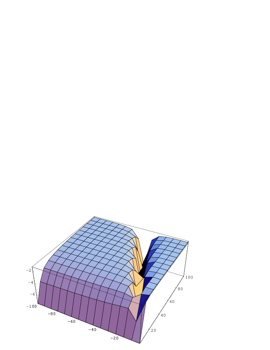
Figure 2: Norm of the states $j=-{1\over 2}-\sqrt{k-7/4}$, as a function of $m<0$ and $k$.

The states have either negative or zero norm. We must stress that this feature arises for the particular states (62) produced from the scattering of one highest weight and one arbitrary tachyon both belonging to the discrete representation.

5 Conclusions

We have studied the factorization properties of scattering amplitudes of $N$-tachyons in the Wakimoto representation of bosonic string theory on $AdS_{3}$. The pole structure appearing when two vertex operators coincide on the world-sheet, reproduces the mass-shell conditions for arbitrarily excited level.

Using the expression for the on-shell three point function computed in reference [14] it is easy to see that the residues are different from zero. By analysing them we were able to obtain the vertex operators creating physical states and study their properties.

The tachyon vertex was reproduced for the ground state. In this case, the mass-shell condition implies that the state produced by the factorization belongs to the principal continuous representation. This is so even though it is possible to avoid this series from the beginning by considering a non trivial contribution to the external states from the internal space.

The vertex operator creating a massless state was found in the particular case when one of the external tachyons which collide to the same point on the world-sheet belongs to the heighest weight representation. The norm of the first excited state produced in this way was computed. It is non-negative independently of the quantum number $m$ and of the level of the algebra $k$ (recall $k\geq 52/23$ in these models). It is interesting to note that the operatorial form (53) is, to this order, the most general one that can couple to tachyons (the coefficients could be more general). In fact, terms containing $\beta$ fields cannot be produced in this way since they lead to violation of the charge conservation conditions which are necessary to obtain a non vanishing result.

Finally we have found the general form of the vertex operator producing a state of the second excited level. Even though we cannot obtain the full vertex operator directly from the factorization we can determine it from the conditions it has to satisfy to be a weight one primary field. The norms of these particular states turn out to be non-positive. Therefore, although we started with unitary external states the interactions introduce ghosts into the theory. This is in accordance with the results found in reference [20] where modular transformations of characters for generic values of $k$ lead to violation of the unitarity bound of string theory on $AdS_{3}$ with a finite number of mass levels.

The procedure which we have developed allows to obtain the general form of the vertex operators for any mass level. At excited level $L$ it can be written as the following sum

$$V^{(L)}_{(j,m)}(z,\bar{z})=\sum_{k,l,n,p=0}^{L}A_{klnp}\phi^{-\delta_{n,0}}\partial^{n}\phi(z)(\partial\phi(z))^{k}\partial^{l}\gamma(z)(\partial\gamma(z))^{p}\gamma^{j-m-p-1}\times c.c.~{}e^{2j\phi/\alpha_{+}}$$ (64)

where $k+l+n+p=L$ and the factor $\phi^{-\delta_{n,0}}$ is included to cancel the contribution $\partial^{0}\phi$.

To conclude, in this paper we have proposed a method and developed the corresponding formalism to study the unitarity of interacting string theory on $AdS_{3}$. Even restricting the external states to those satisfying the unitarity bound the interactions produce negative norm states. These results suggest that the proposed cut off over the values of $j$ should be reconsidered having into account the role of interactions.

Many interesting questions remain. In particular, it is necessary to find a physical mechanism to decouple the ghosts (such as the GSO projection in the superstring theory decouples the tachyons). Otherwise the negative norm states should be interpreted in physical terms as arising from some kind of instability. Moreover it would be interesting to extend this analysis to the supersymmetric case.

Acknowledgements

We would like to thank J. Maldacena, H. Ooguri and J. Russo for many useful discussions and suggestions. This work was supported by CONICET, Argentina, PIP 0873/98.

References

• [1] J. Balog, L. O’Raifeartaigh, P. Forgacs and A. Wipf, Consistency of String Propagation on Curved Space-Times: An SU(1,1) Based Counterexample, Nucl. Phys. B 325 (1989) 225
• [2] P.M.S. Petropoulos, Comments on SU(1,1) String Theory, Phys. Lett. B 236 (1990) 151
• [3] N. Mohammedi, On the Unitary of String Propagation in SU(1,1), Int. J. Mod. Phys. A 5 (1990) 3201
• [4] S. Hwang, No ghost theorem for SU(1,1) string theories, Nucl. Phys. B 354 (1991) 100
• [5] I. Bars and D. Nemeschanshy, String Propagation in Backgrounds with Curved Space-Time, Nucl. Phys. B 348 (1991) 89
• [6] J. Maldacena, The Large N Limit of Superconformal Field Theories and Supergravity, Adv. Theor. Math. Phys. 2 (1998) 231, hep-th/9711200
• [7] A. Giveon, D. Kutasov and N. Seiberg, Comments on String Theory on $AdS_{3}$, Adv. Theor. Math. Phys. 2 (1998) 733, hep-th/9806194
• [8] J. de Boer, H. Ooguri, H. Robins and J. Tannenhauser, String Theory on $AdS_{3}$, JHEP 12 (1998) 026, hep-th/9812046
• [9] D. Kutasov and N. Seiberg, More Comments on String Theory on $AdS_{3}$, JHEP 9904:008 (1999); hep-th/9903219
• [10] I. Bars, Ghost-Free Spectrum of a Quantum String in SL(2,R) Curved Spacetime, Phys. Rev. D 53 (1996) 3308; I. Bars, Solution of the SL(2,R) string in curved space-time, hep-th/ 9511187; I. Bars, C. Deliduman and D. Minic, String Theory on $AdS_{3}$ Revisited, hep-th/9907087
• [11] Y. Satoh, Ghost-free and modular invariant spectra of a string in SL(2,R) and three dimensional black hole geometry, Nucl. Phys. B 513 (1998) 213
• [12] J. M. Evans, M. R. Gaberdiel and M. J. Perry, The No-Ghost Theorem for $AdS_{3}$ and the Stringy Exclusion Principle, hep-th/9806024; The No-Ghost Theorem and Strings on $AdS_{3}$, hep-th/9812252
• [13] G. Aldazabal, M. Bonini, R. Iengo and C. Núñez, Superstring Vertex Operators and Scattering Amplitudes on Arbitrary Riemann Surfaces, Nucl. Phys. B 307 (1988) 291
• [14] M. Becker and K. Becker, Interactions in the SL(2,R)/U(1) Black Hole Background, Nucl. Phys. B 418 (1994) 206, hep-th/9310046; K. Becker,  Strings, Black Holes and Conformal Field Theory, PhD Thesis (1994), hep-th/9404157
• [15] P. Di Francesco and D. Kutasov, World Sheet and Spacetime Physics in Two Dimensional (Super) String Theory, Nucl. Phys. B375 (1992) 119; hep-th/9109005
• [16] M. Wakimoto, Fock Representation of the Affine Lie Algebra A1(1), Comm.Math. Phys. 104 (1986) 605
• [17] A. Gerasimov, A. Morozov, M. Olshanetsky, A. Marshakov and S. Shatashvili, Wess-Zumino-Witten Model as a Theory of Free Fields, Int J. Mod. Phys. A 5 (1990) 2495
• [18] J. Teschner, On Structure Constants and Fusion Rules in the SL(2,C)/SU(2) WZNW Model, hep-th/9712256
• [19] V.S. Dotsenko and V.A. Fateev, Four-Point Correlation Function and the Operator Algebra in the 2D Conformal Invariant Theories with Central Charge $c<1$, Nucl. Phys. B 251 (1985) 691; V.S. Dotsenko and V.A. Fateev, Conformal Algebra and Multipoint Correlation Function in the 2D Statistical Models, Nucl. Phys. B 240 (1984) 312
• [20] P. M. Petropoulos, String Theory on $AdS_{3}$: Some Open Questions, hep-th/9908189