UFIFT-HEP-99-15

hep-th/9909141

QCD Fishnets Revisited

Klaus Bering, Joel S. Rozowsky and Charles B. Thorn

Institute for Fundamental Theory
Department of Physics, University of Florida, Gainesville, FL 32611

()

We look back at early efforts to approximate the large $N_{c}$ Feynman diagrams of QCD as very large fishnet diagrams. We consider more carefully the uniqueness of rules for discretizing $P^{+}$ and $ix^{+}$ which fix the fishnet model in the strong ’t Hooft coupling limit, and we offer some refinements that allow more of the crucial QCD interactions to be retained in the fishnet approximation. This new discretization has a better chance to lead to a physically sensible “bare QCD string” model. Not surprisingly the resulting fishnet diagrams are both richer in structure and harder to evaluate than those considered in older work. As warm-ups we analyze arbitrarily large fishnets of a paradigm scalar cubic theory and very small fishnets of QCD.

Copyright 2000 by The American Physical Society

1 Introduction

With all the recent effort devoted to the search for a solution of large $N_{c}$ QCD [1] as a classical string theory [2], it is appropriate to reassess earlier efforts to accomplish this goal. In this article we wish to refine and extend the formulation and calculational methods developed in the effort of the late seventies to systematize a fishnet [3] approximation to large $N_{c}$ QCD [4, 5].

The larger goal here is to set up a discrete model of infinite $N_{c}$ QCD which, when analyzed in a weak coupling expansion ($N_{c}g^{2}\ll 1$), reproduces perturbative QCD and, when analyzed in a strong coupling limit ($N_{c}g^{2}\to\infty$), describes what we choose to call a “bare QCD string”. Since QCD is supposed to confine at all values of the ’t Hooft coupling, the infinite $N_{c}$ glueball should actually be noninteracting over the whole range of couplings. However, its composite internal structure is generally expected to be quite complicated, and it is only in the strong ’t Hooft coupling limit that the internal structure of an infinite $N_{c}$ glueball can be as simple as that of the “fundamental string” of string theory. We regard it as an open question whether the bare QCD string can be identified with one of the known fundamental strings or is an entirely novel object. We hope that our efforts will eventually settle this issue. We tentatively identify the bare QCD string with the object whose propagation is described by the so-called fishnet diagrams.

As shown in [4] the fishnet diagrams by no means exhaust the planar diagrams of ’t Hooft’s $N_{c}\to\infty$ limit. Fishnets are certainly planar, but they are also very large in both directions: there are many lines and many interaction vertices. It is natural to try to associate such diagrams with strong ’t Hooft coupling $N_{c}g^{2}\to\infty$, but as with all strong coupling expansions one must first define a cutoff theory which controls the size of the kinetic energy of the system. In [4] the choice was to evaluate all graphs on a light front and simultaneously discretize $P^{+}=(P^{0}+P^{3})/\sqrt{2}$ and $x^{+}=(x^{0}+x^{3})/\sqrt{2}$. In this model the large ’t Hooft coupling limit singled out large fishnet diagrams whose continuum limit was a seamless world sheet. As usual with strong coupling limits this conclusion is highly sensitive to the cutoff model.

What one hopes when resorting to strong coupling methods is that although the limit strongly distorts the quantitative details of the continuum theory, the qualitative physics is shared between the continuum and lattice models for all couplings. In standard lattice gauge theories this hope is usually expressed as requiring that the lattice model exhibit no phase transition as the coupling constant is varied from strong to weak coupling. Probably the most familiar case in which there is a phase transition is “compact QED” whose strong coupling limit shows confinement, but whose continuum limit is a theory of free photons.

Although the existence of a phase transition at finite coupling is usually extremely difficult to detect, it is the case that in some situations our lattice fishnets can be seen to be completely irrelevant to the physics of large but finite coupling. In [4] this possibility was noted in the context of scalar $\lambda\phi^{4}$ theory. The qualitative physics of the seamless fishnet diagrams is that the quanta of the field theory are bound into a linear polymeric chain. However, one can examine at next order in the strong coupling expansion the nature of the interaction that should be responsible for this binding. For $\lambda>0$ this interaction is repulsive, and the seamless world sheet given by the strong coupling limit is a purely formal artifact. In contrast, for $\lambda<0$ the interaction is attractive, and it is qualitatively correct to imagine that the nearest neighbor quanta form very tight bonds in the strong coupling limit.

A serious shortcoming of the QCD fishnet model attempted in [5] is that the basic gluon-gluon quartic interaction retained in the strong coupling limit favored the alignment of the gluon spins. This defect was not apparent, however, because the leading fishnet structure was explicitly an even function of this interaction and in fact described an anti-ferromagnetic spin arrangement. The inherent instability of the system would only be seen at non-leading order. We aim to improve this situation in the present work by proposing a discretized model whose fishnet approximation retains both the “contact” interactions, with their ferromagnetic tendency, and the one gluon exchange interactions with their anti-ferromagnetic tendency.

The rest of the article is organized as follows. In Section 2 we give a self contained review of the Feynman rules in light-cone gauge as well as the discretization rules largely following [4, 5]. However, we treat the longitudinal modes differently. We represent the “induced quartic interaction” of light-cone gauge by the exchange of a short-lived fictitious spin 0 quantum: its propagation is limited to a small number of discrete time steps. This idea motivated another departure from [5]. Namely, we also choose to represent the basic quartic gluon interaction by the exchange of another short-lived fictitious spin 0 quantum. In this way all vertices of the discretized Feynman rules are cubic, and are accordingly all treated on the same footing in the strong coupling limit. In Section 3 we show our discretization in action by computing the gluon self energy at one loop order. We see how the ambiguities inherent in spreading out the quartic vertices begin to be resolved by requiring Lorentz invariance. The propagators of the fictitious scalars are multiplied by $f_{k}$, $h_{k}$, where $k$ is the number of time steps, and $\sum_{k}f_{k}=\sum_{k}h_{k}=1$. Lorentz invariance of the self-energy constrains the moments $\sum_{k}f_{k}/k$ and $\sum_{k}h_{k}/k$. In Section 4 we describe the fishnet approximation. As a warm-up, we give a complete analysis of the leading fishnet diagrams of a paradigm matrix scalar field theory $g{\rm Tr}\phi^{3}$. Then we describe the more complicated situation of QCD. We do not attempt to analyze the arbitrary QCD fishnets here. Instead in Section 5 we study the sum of planar diagrams for small values of $M$, the number of units of $P^{+}$ carried by the evolved system. Finally in Section 6 we collect some concluding remarks and sketch future directions for this program of research.

2 Light-cone Feynman Rules and Discretization

2.1 Propagators

The gluon propagator in light-cone gauge $A_{-}=0$ is given in momentum space by

$${\tilde{D}}^{\mu\nu}(p)=-i{\eta^{\mu\nu}-\eta^{\mu+}p^{\nu}/p^{+}-\eta^{+\nu}p^{\mu}/p^{+}\over p^{2}-i\epsilon}.$$ (1)

The signature of our metric tensor $\eta_{\mu\nu}$ is taken to be $(-,+,+,+)$. In this paper we shall make extensive use of the $x^{+}$ representation

$$D^{\mu\nu}({\bf p},p^{+},x^{+})\equiv\int{dp^{-}\over 2\pi}{\tilde{D}}^{\mu\nu}(p)e^{-ix^{+}p^{-}}.$$ (2)

Evaluating the $p^{-}$ integral leads to the following expressions for the individual components of $D^{\mu\nu}$:

$$D^{kl}({\bf p},p^{+},x^{+}) = \theta(x^{+}){\eta^{kl}\over 2p^{+}}e^{-ix^{+}{\bf p}^{2}/2p^{+}}\,\to\,\theta(\tau){\eta^{kl}\over 2p^{+}}e^{-\tau{\bf p}^{2}/2p^{+}}$$

$$D^{k-}({\bf p},p^{+},x^{+}) = \theta(x^{+}){p^{k}\over 2p^{+2}}e^{-ix^{+}{\bf p}^{2}/2p^{+}}\,\to\,\theta(\tau){p^{k}\over 2p^{+2}}e^{-\tau{\bf p}^{2}/2p^{+}}$$

$$D^{--}({\bf p},p^{+},x^{+}) = i{\partial\over\partial x^{+}}\theta(x^{+}){1\over p^{+2}}e^{-ix^{+}{\bf p}^{2}/2p^{+}}\,\to\,-{\partial\over\partial\tau}\theta(\tau){1\over p^{+2}}e^{-\tau{\bf p}^{2}/2p^{+}}$$ (3)

$$= \left[\theta(x^{+}){{\bf p}^{2}\over 2p^{+3}}+i\delta(x^{+}){1\over p^{+2}}\right]e^{-ix^{+}{\bf p}^{2}/2p^{+}}$$

$$\qquad\to\,\left[\theta(\tau){{\bf p}^{2}\over 2p^{+3}}-\delta(\tau){1\over p^{+2}}\right]e^{-\tau{\bf p}^{2}/2p^{+}},$$

where the arrows indicate the imaginary time versions ($\tau=ix^{+}$). In this paper latin indices will always refer to the transverse components. We shall also find it convenient to use a complex basis for transverse indices, defining $V^{\wedge}\equiv(V^{1}+iV^{2})/\sqrt{2}$ and $V^{\vee}\equiv(V^{1}-iV^{2})/\sqrt{2}$. In this basis the metric has values $\eta_{\vee\vee}=\eta_{\wedge\wedge}=0$ and $\eta_{\vee\wedge}=\eta_{\wedge\vee}=1$.

Here we are assuming that $A^{-}=-A_{+}$ has not been eliminated from the formalism. Since Gauss’ law relates $A_{+}$ to the transverse components through a constraint not involving time derivatives, it is possible to explicitly integrate $A_{+}$ out (see for example [6]) leaving the transverse components as the only independent variables. In that case the Feynman rules would only employ the transverse propagator $D^{kl}$. Graphically, one achieves the same result by showing that the contributions of $D^{k-}$ and $D^{--}$ lead to modified cubic vertices and a new induced quartic vertex which arises from the $\delta(x^{+})$ term in $D^{--}$.

2.2 Vertices

$\begin{array}[c]{c}\psfig{height=36.135pt}\end{array}$	$\Gamma_{3}^{\wedge\wedge\wedge}=\Gamma_{3}^{\vee\vee\vee}=0$	$\begin{array}[c]{c}\psfig{height=43.36243pt}\end{array}$	$\Gamma_{3}^{\wedge\wedge\vee}=-g(Q_{2}-Q_{1})^{\wedge}$
$\begin{array}[c]{c}\psfig{height=43.36243pt}\end{array}$	$\Gamma_{3}^{\wedge\vee+}=\Gamma_{3}^{\vee\wedge+}=g(Q_{2}-Q_{1})^{+}$	$\begin{array}[c]{c}\psfig{height=43.36243pt}\end{array}$	$\Gamma_{3}^{\vee\vee\wedge}=-g(Q_{2}-Q_{1})^{\vee}$
$\begin{array}[c]{c}\psfig{height=36.135pt}\end{array}$	$\Gamma_{4}^{\wedge\wedge\vee\vee}=+g^{2}$	$\begin{array}[c]{c}\psfig{height=36.135pt}\end{array}$	$\Gamma_{4}^{\wedge\vee\wedge\vee}=-2g^{2}$

Figure 1: Cubic and quartic gauge vertices for imaginary time.

We shall present the primitive cubic and quartic vertices as ’t Hooft did in his presentation of the $1/N_{c}$ expansion [1]. Since the vertex assignments lack permutation symmetry, it is understood that all permutations of them must be included. The double line notation makes clear what powers of $N_{c}$ must be included with each topology. However, since we shall be dealing exclusively with the planar diagrams of the $N_{c}\to\infty$ limit, we shall dispense with this refinement in order to reduce clutter. To correctly use these rules at finite $N_{c}$, the double line notation should be restored. With this understanding, the primitive cubic vertices are given by

$$\Gamma_{3}^{\vee\vee\vee} = \Gamma_{3}^{\wedge\wedge\wedge}=0$$

$$\Gamma_{3}^{\wedge\wedge\vee} = -ig(Q_{2}-Q_{1})^{\wedge}\to-g(Q_{2}-Q_{1})^{\wedge}$$

$$\Gamma_{3}^{\vee\vee\wedge} = -ig(Q_{2}-Q_{1})^{\vee}\to-g(Q_{2}-Q_{1})^{\vee}$$

$$\Gamma_{3}^{\vee\wedge+} = \Gamma_{3}^{\wedge\vee+}=+ig(Q_{2}-Q_{1})^{+}\to+g(Q_{2}-Q_{1})^{+},$$ (4)

and the primitive quartic vertices by

$$\Gamma_{4}^{\wedge\wedge\vee\vee} = +ig^{2}\to+g^{2}$$

$$\Gamma_{4}^{\wedge\vee\wedge\vee} = -2ig^{2}\to-2g^{2},$$ (5)

where the arrows indicate the appropriate vertices to use with imaginary time. In light-cone gauge, only transverse gluons participate in the quartic vertices. Our convention will be that all momenta flow into the vertex. Also, the index $\vee$ ($\wedge$) will be represented graphically by attaching an outgoing (incoming) arrow to a line (see Fig. 1). The ordering of indices will be counterclockwise around the vertex. As usual, each vertex is associated with an integration over $x^{+}$ and conserves the transverse and $+$ components of momentum. Then each unconstrained momentum is integrated with measure $d^{2}pdp^{+}/(2\pi)^{3}$.

2.3 Discretization

To give a nonperturbative model for the summation over planar diagrams, it was proposed in Ref. [4] to simultaneously discretize $p^{+}=lm$ and imaginary time $\tau\equiv ix^{+}=ka$, with $k,l$ running over all positive integers. The use of imaginary time converts all oscillating exponentials to damped ones, and removes all $i$’s from the Feynman rules. Thus the $i$ occurring in each vertex is combined with the $dx^{+}$ to form $d\tau$. (Because of time translational invariance, the time integral for one vertex in each connected diagram should be omitted, leaving one factor of $i$ unabsorbed. Conventionally, we shall omit this last $i$ in the quantities we calculate.)

It can be easily seen that the lattice constants $a,m$ only enter the sum of graphs in the ratio $T_{0}\equiv m/a$. First notice that only this ratio appears in the exponents. Since each propagator is nominally integrated over its $p^{+}$, $\int dp^{+}\to m\sum$ provides a factor of $m$ to cancel one from a $1/p^{+}$ prefactor in each propagator. Further $\int d\tau\to a\sum$ at each vertex which also has a nominal $p^{+}$ conserving delta function that supplies a $1/m$, so each vertex supplies a factor $1/T_{0}$. Finally, every $-$ index of a propagator will be matched with a $+$ index of a vertex, which will involve a factor of $p^{+}$ and hence supply a factor of $m$ to cancel the extra factor of $1/m$ in $D^{k-}$ and to convert the extra factor of $1/ma$ in $D^{--}$ to $T_{0}$.

The discretization of $D^{--}$ involves some ambiguity in the interpretation of the term involving $\delta(x^{+})$. With $x^{+}$ continuous, this term collapses the two cubic vertices it connects into an instantaneous quartic interaction local in ${\bf x}$ but $p^{+}$ dependent and hence nonlocal in $x^{-}$. Indeed this is precisely the well-known quartic vertex induced by elimination of $A_{+}$ in the Hamiltonian formulation of light-cone gauge. In this approach the remaining part of $D^{--}$ combines nicely with the contributions of $D^{k-}$ to yield a modified cubic vertex for transverse gluons only:

$${\hat{\Gamma}}_{3}^{\wedge\wedge\vee}=-2g\left({Q^{+}_{1}+Q^{+}_{2}\over Q^{+}_{1}Q^{+}_{2}}\right)(Q^{+}_{1}Q^{\wedge}_{2}-Q^{+}_{2}Q^{\wedge}_{1})$$

$${\hat{\Gamma}}_{3}^{\vee\vee\wedge}=-2g\left({Q^{+}_{1}+Q^{+}_{2}\over Q^{+}_{1}Q^{+}_{2}}\right)(Q^{+}_{1}Q^{\vee}_{2}-Q^{+}_{2}Q^{\vee}_{1}),$$ (6)

which are the vertices appropriate to imaginary time. With longitudinal gauge fields completely eliminated in this way, discretization could then proceed as usual by discretizing the $x^{+}$ and $p^{+}$ parameters of the transverse gluon propagator. In addition, one has to exclude, in some ad hoc manner, the $p^{+}=0$ exchange part of the induced quartic vertex which is infinite as it stands. Moreover, the set of “tadpole diagrams” necessarily excluded in our discretization (see Sec. 2.4 below) is enlarged by the induced quartic interaction and, since the new quartic interactions depend non-trivially on $p^{+}$, the $p^{+}$ dependence of the necessary counter-terms will be more complicated. Nevertheless, an attractive feature of such a treatment is that the modified cubic vertex is manifestly invariant under the light-cone Galilei group: ${\bf Q}\to{\bf Q}+Q^{+}{\bf V}$.

We shall follow a different path, more in the spirit of the sum over histories. The idea is to exploit our discretization of $x^{+}$ to give a more flexible interpretation of $\delta(x^{+})$, which retains a Gaussian damping factor and maintains Galilei invariance throughout. This can be done by the replacement:

$$D^{--}({\bf Q},Q^{+}=Mm,x^{+}=-ika) \to {{\bf Q}^{2}\over 2M^{3}}e^{-k{\bf Q}^{2}/2MT_{0}}-f_{k}{T_{0}\over M^{2}}e^{-k{\bf Q}^{2}/2MT_{0}}$$

$$\sum_{k>0}f_{k} = 1.$$ (7)

The last term on the r.h.s. of Eq (2.3) is a satisfactory discretization of the delta function provided the $f_{k}$’s fall off sufficiently rapidly with $k$. The exclusion of $f_{0}$ ensures damping of transverse momentum integrals. In this approach, instead of a new induced quartic vertex we have introduced a short lived scalar, whose exchange simulates that vertex in a way that maintains Galilei invariance. Further, by leaving the choice of the $f_{k}$’s open we might be able to tune their values to cancel unwanted symmetry violations induced by ultraviolet divergences in the continuum limit. The first term on the r.h.s. of Eq (2.3) is exactly what is needed to complete the modified cubic vertex (6) when combining all of the contributions of the longitudinal gluons.

Perhaps a more intuitive discretization would be to replace the derivative in $D^{--}$ by a discrete difference:

$$D^{--}({\bf Q},Mm,-ika) \to -{T_{0}\over M^{2}}\cases{e^{-k{\bf Q}^{2}/2MT_{0}}-e^{-(k-1){\bf Q}^{2}/2MT_{0}}&$k>1$\cr e^{-{\bf Q}^{2}/2MT_{0}}&$k=1$},$$ (8)

where the special treatment of the case $k=1$ simulates the $\delta(x^{+})$ contribution we know must be there in the continuum. Unfortunately, this definition violates Galilei invariance because of the term that propagates only $k-1$ steps in time: Newtonian mass conservation is temporarily violated. This causes considerable complications in calculations, but nonetheless displays interesting features. We will not pursue this option in the main text, but in an appendix we shall see that with a suitable counter-term Galilei invariance of the one loop self energy can be restored in the continuum limit.

2.4 Tadpoles

The exclusion of the propagators with zero $\tau$ and zero $p^{+}$ renders every Feynman integral finite, making our discretization an effective regulator of divergences. But it also means that certain “tadpole” Feynman diagrams, which involve one or more propagators originating and terminating at the same vertex are excluded. In a theory with at most quartic vertices, these diagrams are limited to self-energy parts, which generally require counter-terms to enforce Lorentz invariance in the continuum limit. Thus errors induced by excluding these diagrams could simply be absorbed in the ultimate value of the counter-terms.

Figure 2: Tadpoles Feynman diagrams coming from cubic and quartic vertices.

Tadpoles arising from the cubic interaction (see Fig. 2(a)) represent the vacuum expectation value of the color current density. The transverse components of these would vanish anyway because they are linear in transverse momentum but we can make sure all these tadpoles vanish by simply normal ordering the current density. However tadpoles arising from the quartic interaction, see Fig.2(b), would give a divergent non-vanishing result if the zero time propagator were inserted. As mentioned above one possibility is to absorb them in the self-energy counter-term.

Figure 3: Quartic vertices get replaced by two cubic vertices and a fictitious scalar field.

Another possibility is to note that, from the point of view of the continuum, one can just as well spread the quartic interaction over several time steps, in which case a candidate for the tadpole diagrams would emerge. We have already exploited this idea in our discretization of $D^{--}$, see Eq (2.3). A natural way to do this is to imagine that the quartic interaction is actually the concatenation of two cubic interactions mediated by a fictitious scalar field which is only allowed to propagate a few time steps. We thus redraw the various quartic vertices as in Fig. 3. The fictitious scalars must be “ghosts”: to reproduce the quartic couplings, either their coupling to two transverse gluons must be taken imaginary or their propagator must be negative. We choose the second alternative for which the vertices are given in Fig. 4.

$\begin{array}[c]{c}\psfig{height=43.36243pt}\end{array}$	$\Gamma_{m}^{\wedge\vee}=+{g\over T_{0}}$	$\begin{array}[c]{c}\psfig{height=43.36243pt}\end{array}$	$\Gamma_{m}^{\vee\wedge}=-{g\over T_{0}}$

Figure 4: The couplings of the transverse components of the gauge field to the fictitous scalar field. The subscript $m$ indicates that this is a magnetic ghost vertex. These replace the two quartic vertices at the bottom of Fig. 1.

Note that the quartic vertex which involves adjacent like direction spins in one channel can be viewed as a spin zero exchange in only one way, whereas the vertex with unlike adjacent spins in both channels becomes two exchange diagrams, giving a natural interpretation of the factor of 2 in the effective quartic vertex. If we now consider the “tadpoles” arising from connecting any pair of external lines, we see that there are 3 diagrams, see Fig. 5, but the two with the topology of a cubic tadpole, which cannot be drawn in our discretized light-cone formalism, cancel. Thus the only remaining tadpole is the bubble diagram on the far right of Fig. 5, which poses no problem for our formalism.

Figure 5: Three tadpole diagrams resulting from the spreading out of the quartic gauge vertex.

The fictitious scalar propagator can be taken to be

$$D({\bf Q},M,k) = -h_{k}T_{0}e^{-k{\bf Q}^{2}/2MT_{0}}$$

$$\sum_{k>0}h_{k} = 1,$$ (9)

where the $h_{k}$’s, like the $f_{k}$’s, vanish rapidly with $k$. The normalization condition guarantees that the correct quartic vertex will be reproduced in the continuum limit. The exponential factor damps ultraviolet divergences, and with the form we have specified, maintains Galilei invariance even for finite lattice constants. Furthermore, by leaving the choice of the $h_{k}$’s open, we gain additional flexibility to cancel unwanted symmetry violations. The hope is that tuning the $f_{k}$’s and $h_{k}$’s will remove the need for explicit counter-terms.

3 Gluon Self-energy and Counter-terms at One Loop

In this section we illustrate the way discretization regulates divergences by computing the one-loop contribution to the gluon self-energy part, $i\Pi^{\mu\nu}$, defined as the sum of all one particle irreducible diagrams for the two-point function. For this purpose it is convenient to pass from $x^{+}$ representation to energy ($E=p^{-}$) representation. With discretized $\tau$, this is accomplished by defining

$${\tilde{D}}^{\mu\nu}({\bf Q},M,E) = \sum_{k=1}^{\infty}e^{akE}D^{\mu\nu}({\bf Q},M,k)$$ (10)

$${\tilde{\Pi}}^{\mu\nu}({\bf Q},M,E) = \sum_{k=1}^{\infty}e^{akE}\Pi^{\mu\nu}({\bf Q},M,k).$$ (11)

The exact gluon propagator is then algebraically related to the the bare one and ${\tilde{\Pi}}$. We define $u\equiv e^{-Q^{2}/2MT_{0}}=e^{aE-{\bf Q}^{2}/2MT_{0}}$, in terms of which the bare propagators have the values:

$${\tilde{D}}_{0}^{ij}({\bf Q},M,E) = {\eta^{ij}\over 2M}{u\over 1-u}$$

$${\tilde{D}}_{0}^{i-}({\bf Q},M,E) = {Q^{i}\over 2M^{2}}{u\over 1-u}.$$ (12)

For $D^{--}$ we have, for the discretization of Eq (2.3),

$${\tilde{D}}_{0}^{--}({\bf Q},M,E) = {{\bf Q}^{2}\over 2M^{3}}{u\over 1-u}-{T_{0}\over M^{2}}\sum_{k>0}f_{k}u^{k}.$$ (13)

Because of light-cone gauge, only $\Pi^{ij},\Pi^{i+}$ and $\Pi^{++}$ are required. By transverse rotational invariance, these quantities can be decomposed as

$${\tilde{\Pi}}^{ij} = Q^{i}Q^{j}\Pi_{1}+\eta^{ij}\Pi_{2}$$

$${\tilde{\Pi}}^{i+} = MQ^{i}\Pi^{\prime}_{1}$$

$${\tilde{\Pi}}^{++} = M^{2}\Pi^{\prime\prime}_{1}$$ (14)

We shall find that at the one-loop approximation, $\Pi^{\prime\prime}_{1}=\Pi^{\prime}_{1}=\Pi_{1}$ and if that were to hold generally, the exact propagators would be given by

$${\tilde{D}}^{ij} = {\eta^{ij}\over 2M}{u\over 1-u-u\Pi_{2}/2M}$$

$${\tilde{D}}^{i-} = {Q^{i}\over 2M^{2}}{u\over 1-u-u\Pi_{2}/2M}$$

$${\tilde{D}}^{--} = {T_{0}\over M^{2}}\left[{-\sum_{k}f_{k}u^{k}\over 1+T_{0}\Pi_{1}\sum_{k}f_{k}u^{k}}+{{\bf Q}^{2}\over 2MT_{0}}{u\over 1-u-u\Pi_{2}/2M}\right].$$ (15)

3.1 Calculation of $\Pi_{1}$

Figure 6: The two bubble diagrams that contribute to $\Pi^{++}$.

After these preliminaries, let us now turn to the computation of $\Pi_{1}$ at one loop. The simplest term is $\Pi^{++}$, which is given in $x^{+}$ representation by (note that there are 2 equal diagrams that contribute (see Fig. 6))

$$\Pi^{++} = 2{g^{2}N_{c}\over T_{0}^{2}}\int{d^{2}p\over(2\pi)^{3}}\sum_{l=1}^{M-1}{(M-2l)^{2}\over 4l(M-l)}e^{-k({\bf p}^{2}/2l+({\bf Q}-{\bf p})^{2}/2(M-l))/T_{0}}$$ (16)

$$= {2g^{2}N_{c}\over 16\pi^{2}T_{0}}\sum_{l=1}^{M-1}{(M-2l)^{2}}{1\over Mk}e^{-k{\bf Q}^{2}/2MT_{0}}={N_{c}g^{2}(M-1)(M-2)\over 24\pi^{2}T_{0}k}e^{-k{\bf Q}^{2}/2MT_{0}}$$

$${\tilde{\Pi}}^{++} = {g^{2}N_{c}\over 24\pi^{2}T_{0}}(M-1)(M-2)(-\ln(1-u)).$$ (17)

Figure 7: The four bubble diagrams that contribute to $\Pi^{\wedge+}$.

The evaluation of $\Pi^{j+}$ is not much harder. Here there are four diagrams that differ only in the prefactor of transverse momentum (see Fig. 7). Since the prefactor is linear in momentum, we need only to remember that the Gaussian integral over transverse momentum involves the shift ${\bf p}\to{\bf p}+l{\bf Q}/M$. After this shift the term linear in $\bf p$ integrates to zero, so the net effect is to set ${\bf p}=l{\bf Q}/M$. Thus the net prefactor is

$${Q^{j}\over M}(2l-M)[(1+l/M)+(-2+l/M)+\eta_{+-}(-1-l/M)+\eta_{+-}(2-l/M)]={2Q^{j}\over M^{2}}(2l-M)^{2},$$ (18)

which involves the identical sum over $l$ as $\Pi^{++}$. Thus we end up with

$${\tilde{\Pi}}^{j+} = {g^{2}N_{c}\over 24\pi^{2}T_{0}}{Q^{j}\over M}(M-1)(M-2)(-\ln(1-u)).$$ (19)

Figure 8: The eight bubble diagrams that contribute to $\Pi^{\wedge\wedge}$.

The coefficient of $Q^{i}Q^{j}$ in $\Pi^{ij}$ may be singled out by computing $\Pi^{\wedge\wedge}$. This leads to a similar calculation to the above because, after the shift in integration variable, $p^{\wedge}$ and $p^{\wedge}p^{\wedge}$ both integrate to zero. Thus again, prefactors of $p^{\wedge}$ may simply be set to $lQ^{\wedge}/M$. Eight diagrams contribute to this quantity, equal in pairs (see Fig. 8). The prefactors of these diagrams combine as follows:

$$\hskip-5.69046pt{2Q^{\wedge}Q^{\wedge}\over M^{2}}((M+l)^{2}+(2M-l)^{2}-(M+l)(2M-l)-(M+l)(2M-l))={2Q^{\wedge}Q^{\wedge}\over M^{2}}(2l-M)^{2}.$$ (20)

So again we have the same sum over $l$, leading to:

$$\Pi^{\wedge\wedge}={g^{2}N_{c}\over 24\pi^{2}T_{0}}{Q^{\wedge}Q^{\wedge}\over M^{2}}(M-1)(M-2)(-\ln(1-u)).$$ (21)

The upshot of the calculations so far is that

$$\Pi_{1}=\Pi_{1}^{\prime}=\Pi_{1}^{\prime\prime}={g^{2}N_{c}\over 24\pi^{2}T_{0}}(1-{3\over M}+{2\over M^{2}})(-\ln(1-u)).$$ (22)

The equality of the various $\Pi$’s holds even at finite $m,a$. This can be understood because the diagrams we have evaluated show no violation of Galilei invariance. Our result for $\Pi_{1}$ can be compared with the result from the study of asymptotic freedom in the infinite momentum frame [8]:

$$\Pi_{1}(Q^{2})={g^{2}N_{c}\over 24\pi^{2}}\left(\ln{\Lambda^{2}\over Q^{2}}+12\right),$$ (23)

in which a simple cutoff ${\bf k}^{2}<\Lambda^{2}$ was employed. To make the comparison, note that in the continuum limit, $a\to 0,M\to\infty$, $1-u\approx({\bf Q}^{2}-2Q^{+}E)/2MT_{0}=Q^{2}/2MT_{0}$. Thus for us, the role of $\Lambda^{2}$ is played by the quantity $2MT_{0}=2Q^{+}/a$. Note that if we choose to keep $T_{0}$ fixed, the ultraviolet cutoff is removed by simply taking $M\to\infty$.

3.2 Calculation of $\Pi_{2}$

Finally we turn to the real core of the self energy calculation, the determination of $\Pi_{2}$, which can be inferred from $\Pi^{\wedge\vee}=Q^{\wedge}Q^{\vee}\Pi_{1}+\Pi_{2}=\Pi_{2}+{\bf Q}^{2}\Pi_{1}/2$. Seventeen diagrams contribute to this quantity, fifteen of which do not involve $D^{--}$ and are relatively simple to analyze.

Figure 9: The three bubble diagrams that contribute to $\Pi^{\wedge\vee}_{\rm A}$ involving only transverse components.

First consider the three diagrams that only involve transverse internal propagators (see Fig. 9). The prefactors of transverse momentum combine as follows:

$$(2p-Q)^{\wedge}(2p-Q)^{\vee}+(p+Q)^{\wedge}(p+Q)^{\vee}+(2Q-p)^{\wedge}(2Q-p)^{\vee} = 3({\bf p}^{2}+{\bf Q}^{2}-{\bf p}\cdot{\bf Q})$$

$$\to 3({\bf p}^{2}+(1-l/M+(l/M)^{2}){\bf Q}^{2}),$$ (24)

where in the last line we have indicated the result of shifting ${\bf p}$ by $l{\bf Q}/M$ and dropping the term linear in ${\bf p}$. The transverse integral of the term in ${\bf Q}^{2}$ is the same as before, but the term in ${\bf p}^{2}$ gives an extra factor $2T_{0}l(M-l)/kM$. These terms require the sums

$$\sum_{l=1}^{M-1}(M^{2}-lM+l^{2})={M(M-1)(5M-1)\over 6},\qquad\sum_{l=1}^{M-1}l(M-l)={M(M-1)(M+1)\over 6}$$ (25)

respectively. The contribution of these three diagrams, $\Pi^{\wedge\vee}_{\rm A}$, is given by

$$\Pi^{\wedge\vee}_{\rm A}={g^{2}N_{c}\over 16\pi^{2}}\left[{M^{2}-1\over k^{2}M}+{5M^{2}-6M+1\over 2kM^{2}T_{0}}{\bf Q}^{2}\right]e^{-k{\bf Q}^{2}/2MT_{0}}.$$ (26)

Figure 10: The eight bubble diagrams that contribute to $\Pi^{\wedge\vee}_{\rm B}$.

The next class of diagrams consists of the eight graphs with one $D^{j+}$ propagator, shown in Fig. 10. Remembering the single factor $\eta_{+-}$, we find that the prefactors combine as follows:

$$-(2M-l)\left[{p^{\wedge}\over l}(Q-2p+Q+p)^{\vee}+{p^{\vee}\over l}(Q-2p+Q+p)^{\wedge}\right]$$

$$\qquad-(M+l)\left[{(Q-p)^{\wedge}\over M-l}(-Q+2p+2Q-p)^{\vee}+{(Q-p)^{\vee}\over M-l}(-Q+2p+2Q-p)^{\wedge}\right]$$

$$\qquad\qquad=-{2M-l\over l}{\bf p}\cdot(2{\bf Q}-{\bf p})-{M+l\over M-l}({\bf Q}-{\bf p})\cdot({\bf Q}+{\bf p})$$

$$\qquad\qquad\to-{5M^{2}-2lM+2l^{2}\over M^{2}}{\bf Q}^{2}+{2M^{2}-2lM+2l^{2}\over l(M-l)}{\bf p}^{2}$$ (27)

where as before the arrow indicates the effect on the prefactors after the usual shift of integration variables. Performing the by now familiar integrals and sums leads to the following result for the contribution of this class of eight diagrams, labeled by $\Pi^{\wedge\vee}_{\rm B}$:

$$\Pi^{\wedge\vee}_{\rm B}={g^{2}N_{c}\over 24\pi^{2}}\left[{5M^{2}-6M+1\over k^{2}M}-{14M^{2}-15M+1\over 2kM^{2}T_{0}}{\bf Q}^{2}\right]e^{-k{\bf Q}^{2}/2MT_{0}}.$$ (28)

Combining this with the previous three diagrams yields for the eleven diagrams considered thus far

$$\Pi^{\wedge\vee}_{\rm A}+\Pi^{\wedge\vee}_{\rm B}={g^{2}N_{c}\over 48\pi^{2}}{13M^{2}-12M-1\over M}\left[{1\over k^{2}}-{{\bf Q}^{2}\over 2kMT_{0}}\right]e^{-k{\bf Q}^{2}/2MT_{0}}.$$ (29)

Figure 11: The two bubble diagrams that contribute to $\Pi^{\wedge\vee}_{\rm C}$.

The prefactors in the pair of diagrams (shown in Fig. 11) involving two $D^{j+}$ propagators combine to form

$${(M+l)(l-2M)\over l(M-l)}{\bf p}\cdot({\bf Q}-{\bf p})\to{(M+l)(2M-l)\over l(M-l)}{\bf p}^{2}-{(M+l)(2M-l)\over M^{2}}{\bf Q}^{2}.$$ (30)

This time the required sum is just

$$\sum_{l=1}^{M-1}(2M^{2}+lM-l^{2})=M(M-1)(13M+1)/6,$$ (31)

so that these two diagrams simply double the result of the first eleven. So, in summary, the total contributions of the thirteen diagrams that do not involve $D^{--}$ to $\Pi^{\wedge\vee}$ and ${\tilde{\Pi}}^{\wedge\vee}$ are

$$\Pi^{\wedge\vee}_{\rm A}+\Pi^{\wedge\vee}_{\rm B}+\Pi^{\wedge\vee}_{\rm C}={g^{2}N_{c}\over 24\pi^{2}}{13M^{2}-12M-1\over M}\left[{1\over k^{2}}-{{\bf Q}^{2}\over 2kMT_{0}}\right]e^{-k{\bf Q}^{2}/2MT_{0}}$$ (32)

$${\tilde{\Pi}}^{\wedge\vee}_{\rm A}+{\tilde{\Pi}}^{\wedge\vee}_{\rm B}+{\tilde{\Pi}}^{\wedge\vee}_{\rm C}={g^{2}N_{c}\over 24\pi^{2}}{13M^{2}-12M-1\over M}\left[\sum_{k=1}^{\infty}{u^{k}\over k^{2}}+{{\bf Q}^{2}\over 2MT_{0}}\ln(1-u)\right]$$ (33)

Figure 12: The two bubble diagrams that contribute to $\Pi^{\wedge\vee}_{\rm D}$ which involve a $D^{--}$ propagator.

The two diagrams in Fig. 12, have a $D^{--}$ propagator as one of the internal lines and lead to a qualitatively different evaluation than the first thirteen. Using (2.3) the Gaussian exponents are the same as with the first thirteen diagrams. One finds

$$\Pi^{\wedge\vee}_{\rm D} = {g^{2}N_{c}\over 8\pi^{2}}\sum_{l=1}^{M-1}\left\{{(2M-l)^{2}\over l}e^{-k{\bf Q}^{2}/2MT_{0}}\left[{M-l\over k^{2}M^{2}}-{f_{k}\over Mk}+{l{\bf Q}^{2}\over 2kM^{3}T_{0}}\right]+(l\to M-l)\right\}\qquad\qquad$$ (34)

$$= {g^{2}N_{c}\over 4\pi^{2}}e^{-k{\bf Q}^{2}/2MT_{0}}\bigg{[}{1-kf_{k}\over k^{2}}(4M[\psi(M)+\gamma]-7(M-1)/2)$$

$$-{(M-1)(14M-1)\over 6k^{2}M}+{(M-1)(14M-1){\bf Q}^{2}\over 12kM^{2}T_{0}}\bigg{]},$$

where we have made use of the identity

$${1\over M}\sum_{l=1}^{M-1}{(2M-l)^{2}\over l}=4M[\psi(M)+\gamma]-{7\over 2}[M-1],$$ (35)

where $\psi(z)=\Gamma^{\prime}(z)/\Gamma(z)$ is the digamma function and $\gamma$ is Euler’s constant. At large $M$, we have

$$\psi(M)\sim\ln M-{1\over 2M}-\sum_{n\geq 1}{B_{2n}\over 2nM^{2n}},$$ (36)

where $B_{2n}$ are the Bernoulli numbers.

Figure 13: The two bubble diagrams that contribute to $\Pi^{\wedge\vee}_{\rm E}$ which correspond to the tadpole contributions induced by the spread out quartic vertices.

With the quartic vertices realized as the exchange of a magnetic scalar, we have a definite proposal for the tadpole contribution to the self-energy, namely the two diagrams of Fig. 13, which each give equal contributions. Calling the tadpole contribution $\Pi^{\wedge\vee}_{E}$, we find

$$\Pi^{\wedge\vee}_{E} = -2{g^{2}N_{c}\over(2\pi)^{3}T_{0}}\int d^{2}p\sum_{l=1}^{M-1}{h_{k}\over 2(M-l)}e^{-k[M{\bf p}^{2}/l(M-l)+{\bf Q}^{2}/M]/2T_{0}}$$ (37)

$$= -{g^{2}N_{c}\over 4\pi^{2}}\sum_{l=1}^{M-1}{lh_{k}\over Mk}e^{-k{\bf Q}^{2}/2MT_{0}}$$

$$= -{g^{2}N_{c}\over 8\pi^{2}}(M-1){h_{k}\over k}e^{-k{\bf Q}^{2}/2MT_{0}}$$

Adding $\Pi^{\wedge\vee}_{D}+\Pi^{\wedge\vee}_{E}$ to the first thirteen diagrams, gives (in energy representation)

$${\tilde{\Pi}}^{\wedge\vee} = {\tilde{\Pi}}^{\wedge\vee}_{\rm A}+{\tilde{\Pi}}^{\wedge\vee}_{\rm B}+{\tilde{\Pi}}^{\wedge\vee}_{\rm C}+{\tilde{\Pi}}^{\wedge\vee}_{\rm D}+{\tilde{\Pi}}^{\wedge\vee}_{\rm E}$$ (38)

$$= {g^{2}N_{c}\over 4\pi^{2}}\bigg{[}\sum_{k=1}^{\infty}{u^{k}\over k^{2}}\left(4M[\psi(M)+\gamma]-{(M-1)(11M-1)\over 3M}\right)-\sum_{k=1}^{\infty}h_{k}{u^{k}\over k}{M-1\over 2}$$

$$-\sum_{k=1}^{\infty}f_{k}{u^{k}\over k}\left(4M[\psi(M)+\gamma]-{7(M-1)\over 2}\right)+\sum_{k=1}^{\infty}{u^{k}\over k}{(M-1)(M-2){\bf Q}^{2}\over 12M^{2}T_{0}}\bigg{]}.$$

To get $\Pi_{2}$ we must subtract ${\bf Q}^{2}{\Pi}_{1}/2$, which exactly cancels the last term leaving:

$${\Pi}_{2} = {g^{2}N_{c}\over 4\pi^{2}}\bigg{[}\sum_{k=1}^{\infty}{u^{k}\over k^{2}}\left(4M[\psi(M)+\gamma]-{(M-1)(11M-1)\over 3M}\right)$$ (39)

$$-\sum_{k=1}^{\infty}h_{k}{u^{k}\over k}{M-1\over 2}-\sum_{k=1}^{\infty}f_{k}{u^{k}\over k}\left(4M[\psi(M)+\gamma]-{7(M-1)\over 2}\right)\bigg{]}.$$

The first term inside the large square brackets is exactly the contribution one would obtain using the modified cubic vertex (6) in the three diagrams of Fig. 9. The terms with $f_{k}$ represent the tadpole diagram that would have been constructed from the induced quartic vertex had $A_{+}$ been eliminated from the formalism. This is as it should be because summing over all the diagrams involving $D^{-k}$ and $D^{--}$ is the graphical equivalent of the elimination of the $A_{+}$ degree of freedom. The formalism with $A_{+}$ eliminated gives an extremely efficient calculation of the three bubble diagrams, as shown in the next subsection, but no candidate for the tadpoles. But by treating $A_{+}$ graphically we are led to a useful proposal for the tadpole diagram.

In order to compare our results to the continuum calculation of Ref. [8], we must examine the limits $u\to 1$ and $M\to\infty$. The behavior of the first term of Eq. (39) in this limit is transparent once we use the identity

$$\sum_{k=1}^{\infty}{u^{k}\over k^{2}}={\pi^{2}\over 6}-\ln u\ \ln(1-u)-\sum_{k=1}^{\infty}{(1-u)^{k}\over k^{2}}\approx{\pi^{2}\over 6}+(1-u)(\ln(1-u)-1),$$ (40)

for $u\approx 1$. The last two terms can be expanded about $u=1$:

$$\sum_{k=1}^{\infty}h_{k}{u^{k}\over k} = \sum_{k=1}^{\infty}{h_{k}\over k}+(u-1)\sum_{k=1}^{\infty}h_{k}+{\cal O}((u-1)^{2})$$ (41)

$$= \sum_{k=1}^{\infty}{h_{k}\over k}+(u-1)+{\cal O}((u-1)^{2}),$$

and a similar expansion for $\sum_{k}f_{k}u^{k}/k$. The coefficient of the linear term is completely determined by the normalization conditions on the $f$’s and $h$’s. Momentum independent terms in $\Pi_{2}$ imply a (divergent and noncovariant) tachyonic gluon mass squared in perturbation theory. Since the gluon has only helicity $\pm 1$, such a mass is inconsistent with Poincaré invariance of the continuum limit. Clearly these symmetry violating terms would be cancelled if we could impose the constraints

$$\sum_{k=1}^{\infty}{f_{k}\over k} = {\pi^{2}\over 6}$$ (42)

$$\sum_{k=1}^{\infty}{h_{k}\over k} = -{\pi^{2}\over 18}\left(1-{2\over M}\right),$$ (43)

but clearly the second of these is impossible with $h_{k}$ independent of $M$ (implicitly assumed in (9)). The best we can do is to set the r.h.s. of Eq. (43) to $-\pi^{2}/18$, which would cancel the linear divergence of $\Pi_{2}$. However, there remains a finite gluon mass which is still inconsistent with the Poincaré invariance of the continuum theory. One option would be to cancel this with a mass counter-term, whose coefficient would have to be determined order by order.

Another approach is to allow $h_{k}$ to be dependent on $M$. We have the freedom to make this replacement as long as we recover the correct continuum limit ($M\rightarrow\infty$ and $a\rightarrow 0$) of the theory. With this modification, Eq. (37) is replaced by

$$\Pi^{\wedge\vee}_{E}=-{g^{2}N_{c}\over 4\pi^{2}}\sum_{l=1}^{M-1}{lh_{k}(l)\over Mk}e^{-k{\bf Q}^{2}/2MT_{0}},$$ (44)

where the sum over $l$ is not performed. Similarly Eq.’s (38) and (39) should now include the corrected $\Pi^{\wedge\vee}_{E}$. Thus $\Pi_{2}$ is given by

$${\Pi}_{2} = {g^{2}N_{c}\over 4\pi^{2}}\bigg{[}\sum_{k=1}^{\infty}{u^{k}\over k^{2}}\left(4M[\psi(M)+\gamma]-{(M-1)(11M-1)\over 3M}\right)$$ (45)

$$-\sum_{k=1}^{\infty}u^{k}\sum_{l=1}^{M-1}{lh_{k}(l)\over Mk}-\sum_{k=1}^{\infty}f_{k}{u^{k}\over k}\left(4M[\psi(M)+\gamma]-{7(M-1)\over 2}\right)\bigg{]},$$

and the expansion of Eq. (41) about $u=1$ should now be

$$-\sum_{k=1}^{\infty}u^{k}\sum_{l=1}^{M-1}{lh_{k}(l)\over Mk} = -\sum_{k=1}^{\infty}\sum_{l=1}^{M-1}{lh_{k}(l)\over Mk}-(u-1)\sum_{k=1}^{\infty}\sum_{l=1}^{M-1}{lh_{k}(l)\over M}+{\cal O}((u-1)^{2})$$ (46)

$$= -\sum_{k=1}^{\infty}\sum_{l=1}^{M-1}{lh_{k}(l)\over Mk}-(u-1){M-1\over 2}+{\cal O}((u-1)^{2}).$$

The constraint equation that replaces (43) is

$$\sum_{l=1}^{M-1}{l\over M}\sum_{k=1}^{\infty}{h_{k}(l)\over k}=-{(M-1)(M-2)\over 6M}{\pi^{2}\over 6},$$ (47)

which can be satisfied if we require

$$\sum_{k=1}^{\infty}{h_{k}(l)\over k} = -{\pi^{2}\over 18}\left(1-{1\over l}\right).$$ (48)

We prefer this approach to that of a mass counter-term, since it is possible that this is a uniform description that works order by order (at each order the cancellation places constraints on higher moments of $h$). The hope is that this can be used non-perturbatively.

In the continuum limit $M(1-u)\to Q^{2}/2T_{0}$ stays finite and we find that $\Pi_{2}$ tends to

$$\Pi_{2}\to{g^{2}N_{c}\over 16\pi^{2}}{Q^{2}\over T_{0}}\left\{\left[8(\ln M+\gamma)-{22\over 3}\right]\ln{Q^{2}\over 2MT_{0}}+{4\over 3}\right\}.$$ (49)

Remembering that our $\Pi_{2}$ is a factor of $-Q^{2}/T_{0}$ times that defined in Ref. [8], we find agreement for the coefficient of $Q^{2}\ln Q^{2}$, provided we identify $Me^{\gamma}$ with $Q^{+}/\epsilon$ and $2MT_{0}$ with $\Lambda^{2}$. We do not get, nor should we expect, the same (finite) coefficient of $Q^{2}$.

3.3 A Brief Calculation of $\Pi$

In the work just completed, we deliberately kept the $A_{+}$ degree of freedom in the graphical rules in order to keep the calculation as close as possible to one in other gauges. However, having seen how all of the graphs with longitudinal gluons combine so nicely, it is appropriate to note that the calculation with $A_{+}$ explicitly eliminated, so that the Feynman rules refer only to the transverse gluons, is much more compact and efficient. With our prescription we can exploit this simplification by using the modified cubic vertices Eq. (6) for the transverse gluons. At the same time we retain our replacement of both the bare and induced quartic vertices by the exchange of two short-lived scalars. The self-energy diagrams involving those scalars will be exactly as described previously (i.e. the terms involving $f$’s and $h$’s). However, all of the remaining contributions to $\Pi^{kl}$ are reduced to the two or three diagrams involving only transverse gluons and the modified cubic vertices.

Only two diagrams contribute to $\Pi^{\wedge\wedge}$, the last two diagrams in Fig. 8, and they each involve a prefactor

$$(Mp-lQ)^{\wedge}(Mp-lQ)^{\wedge}\to M^{2}p^{\wedge}p^{\wedge},$$ (50)

after the shift in momentum. Clearly this integrates to zero so $\Pi^{\wedge\wedge}=0$. Finally there are only three non-tadpole graphs to consider for $\Pi^{\wedge\vee}$, namely those in Fig. 9. In this case the relevant prefactors from the three diagrams contributing to $\Pi^{\wedge\vee}$ combine as

$$2\left[{M^{2}\over l^{2}(M-l)^{2}}+{l^{2}\over(M-l)^{2}M^{2}}+{(M-l)^{2}\over M^{2}l^{2}}\right](M{\bf p}-l{\bf Q})^{2}$$

$$\hskip 72.26999pt\qquad\qquad\to 2\left[{M^{2}\over l^{2}(M-l)^{2}}+{l^{2}\over(M-l)^{2}M^{2}}+{(M-l)^{2}\over M^{2}l^{2}}\right]M^{2}{\bf p}^{2}.$$ (51)

after the usual shift in momentum. Note that because these vertices are manifestly Galilei invariant, there is no term proportional to ${\bf Q}^{2}$ in the prefactor. Thus after integration over loop momentum we are left with the contribution to $\Pi^{\wedge\vee}$:

$$\Pi^{\wedge\vee}_{\rm non-tadpole} = {g^{2}N_{c}\over 4\pi^{2}}{1\over k^{2}}\sum_{l=1}^{M-1}\left[{M^{2}\over l(M-l)}+{l^{3}\over(M-l)M^{2}}+{(M-l)^{3}\over M^{2}l}\right]$$ (52)

$$= {g^{2}N_{c}\over 4\pi^{2}}{1\over k^{2}}\sum_{l=1}^{M-1}\left[{4M\over l}+2{-3M^{2}+3Ml-l^{2}\over M^{2}}\right]$$

$$= {g^{2}N_{c}\over 4\pi^{2}}{1\over k^{2}}M\left[{4(\psi(M)+\gamma})-{11\over 3}+{4\over M}-{1\over 3M^{2}}\right].$$

In this way of organizing the calculation, the longitudinal components of $\Pi^{\mu\nu}$ play no role and the new diagrams contributing to $\Pi^{\wedge\vee}$ give $\Pi_{2}$ directly. For the non-tadpole part we find:

$$\Pi_{2}^{\rm non-tadpole} = {g^{2}N_{c}\over 4\pi^{2}}\sum_{k=1}^{\infty}{u^{k}\over k^{2}}M\left[{4(\psi(M)+\gamma})-{11\over 3}+{4\over M}-{1\over 3M^{2}}\right],$$ (53)

which is clearly a much simpler and more compact calculation! To this result must be added the contribution of the fictitious scalar diagrams, which represent the tadpoles. Needless to say, the calculation of more complicated processes should make use of these new Feynman rules, which we have summarized in Fig. 14.

$\begin{array}[c]{c}\psfig{height=36.135pt}\end{array}$	$0$	$\begin{array}[c]{c}\psfig{height=43.36243pt}\end{array}$	${g\over T_{0}}(M_{2}-M_{1})$
$\begin{array}[c]{c}\psfig{height=43.36243pt}\end{array}$	$-2{g\over T_{0}}\left({M_{1}+M_{2}\over M_{1}M_{2}}\right)(M_{1}Q^{\wedge}_{2}-M_{2}Q^{\wedge}_{1})$	$\begin{array}[c]{c}\psfig{height=43.36243pt}\end{array}$	$+{g\over T_{0}}$
$\begin{array}[c]{c}\psfig{height=43.36243pt}\end{array}$	$-2{g\over T_{0}}\left({M_{1}+M_{2}\over M_{1}M_{2}}\right)(M_{1}Q^{\vee}_{2}-M_{2}Q^{\vee}_{1})$	$\begin{array}[c]{c}\psfig{height=43.36243pt}\end{array}$	$-{g\over T_{0}}$
$\begin{array}[c]{c}\psfig{width=43.36243pt}\end{array}$	${1\over 2M}e^{-k{\bf Q}^{2}/2MT_{0}}$
$\begin{array}[c]{c}\psfig{width=43.36243pt}\end{array}$	$-f_{k}{T_{0}\over M^{2}}e^{-k{\bf Q}^{2}/2MT_{0}}$
$\begin{array}[c]{c}\psfig{width=43.36243pt}\end{array}$	$-h_{k}T_{0}e^{-k{\bf Q}^{2}/2MT_{0}}$

Figure 14: Summary of discretized Feynman rules using only cubic vertices. We have explicitly inserted a factor of $1/T_{0}$ for each vertex arising from the discretization.

4 Summing Planar Diagrams: Fishnets

The discretized Feynman rules given at the end of Sec. 3 provide a tool to sum classes of diagrams. As described in [4] summing diagrams on a light front has a direct interpretation as the path history quantum evolution of a system of particles moving in the transverse space under Newtonian dynamics. By fixing the total discretized $P^{+}=Mm$, the maximum number of particles present at any time is $M$. Because the vertices allow particles to fuse and fission, particle number is not conserved and there is quantum mechanical mixing between states with any number of particles between 1 and $M$.

We are particularly interested in the class of planar diagrams singled out by ’t Hooft’s $N_{c}\to\infty$ limit of QCD. It is actually more precise to think of this class of diagrams as drawn on a cylinder rather than a plane: At any time the system of particles is ordered around a ring, and interactions only exist between neighbors on this ring. Thus the stage is set for the particles to bind into a closed polymer chain. This was previously investigated in [4] where scalar matrix field theory with quartic couplings, $\lambda{\rm Tr}\phi^{4}/4$ was considered. These interactions are attractive (repulsive) if $\lambda<0$ ($\lambda>0$). Thus bound chains can form only if $\lambda<0$, the unstable sign. In the interpretation of the sum of diagrams as a sum over histories of a system of particles, this sign assures that all histories contribute with a positive weight. Using the discretization of $P^{+}$ and $ix^{+}$, as reviewed here in Sec. 2, a strong ’t Hooft coupling limit $\lambda N_{c}\to\infty$ was formulated and analyzed. This was achieved by focusing attention on the cylinder diagrams that evolve a system of particles with $P^{+}=Mm$ a fixed large number $N$ steps forward in time. The limit singles out those diagrams in which every particle has the minimum $P^{+}=m$ (so the number of particles is maximal $=M$), and each propagator evolves only one time step. For even $M$ these diagrams include the large fishnet diagrams that form a seamless web of quartic vertices and propagators, and the resulting Gaussian integrals could be identified as a discretized path integral for a relativistic bosonic string quantized on the light-cone.

This work on scalar field theory was immediately followed by a first attempt to apply these ideas to large $N_{c}$ QCD [5]. In that work QCD was formulated on a light front, with $P^{+}$ and $ix^{+}$ discretized. The ordinary bare vertices of QCD, both cubic and quartic, were used. Because the quartic coupling in QCD is of order $g^{2}$, the literal strong coupling limit, as formulated in [4], favored fishnet diagrams with only the primitive (i.e.  non-induced) quartic couplings. Actually this conclusion required the ad hoc exclusion of the $P^{+}=0$ exchange part of the induced quartic interactions arising from fixing the light-cone gauge. Nonetheless, the resulting fishnet was very interesting: the spin of the gluons played the role of the arrows of a certain six vertex model, known as the F-model [9]. In fact the four gluon vertices of the field theory were exactly the vertices of the F-model. The fact that some of the vertex weights were negative did not cause problems for the leading strong coupling fishnets because those diagrams always had an even number of negative weight vertices. However the problem with them reappears at next order because the deletion of a single negative vertex reveals a repulsive nearest neighbor interaction in that spin channel. Thus that channel could not have formed a bond in the first place. In some spin channels there were also positive weights, so that the bonds could form. However, unfortunately for these fishnets, the attractive channels are ferromagnetic: the only long polymers that could be formed by these interactions would have enormous spin!

The problem is that at strong coupling only the quartic interactions survived with the discretization of [5]. The spin-spin interaction from gluon exchange has anti-ferromagnetic behavior, and it is possible that a discretization that allowed the exchange interaction to compete with the quartic interaction could cure this problem. To explore this possibility, one of us examined the relative strengths of quartic and cubic exchange interactions for neighbors on a gluonic chain by putting the two gluons in a spherical MIT bag [10]. In that context one can see explicitly, not only that the cubic exchange of a transverse gluon is anti-ferromagnetic, but that its strength (at least in weak coupling perturbation theory) is more than sufficient to reverse the ferromagnetic character of the quartic interaction. A major shortcoming of the discretization of [5] is that at strong coupling the cubic interactions have no opportunity to compete with the quartic interactions.

The discretization developed in Sec. 2 of this paper is more promising. In fact, we do away with quartic interactions completely: All interactions are cubic! The quartic interactions have been replaced by the exchange of fictitious scalars, and these exchanges are not enhanced by strong coupling over the exchanges of the ordinary transverse gluons. Without quartic vertices the basic cells of the densest diagrams are no longer square but hexagonal: the fishnet looks like a honeycomb (see Fig. 15).

Figure 15: Hexagonal cell fishnet made of only cubic vertices. The dashed lines indicate the closed cylindrical topology.

These fishnet diagrams require particles with both 1 and 2 units of $P^{+}$. Thus the leading fishnet structure is somewhat looser than in the quartic coupling case. The inclusion of two different values of $P^{+}$ in the leading approximation also sets the stage for the emergence of a string degree of freedom (provided string states do form!) corresponding to fluctuations in $P^{+}$. Such a degree of freedom is expected to be described at long worldsheet wavelength by Polyakov’s Liouville field [11].

Because all of our vertices are cubic, the paradigm scalar field theory is now $g{\rm Tr}\phi^{3}/3$ (see [12] for a discussion of this model in $1+1$ dimensions). Of course, the presence of factors of transverse momentum in the QCD cubic vertices will cause a profound qualitative difference between gauge and scalar theory. For one thing, the scalar theory is super-renormalizable with the cubic coupling carrying dimensions of mass. This means that weak or strong coupling is determined by the size of the ratio $g^{2}N_{c}/\mu^{2}$, where $\mu$ is a mass scale relevant to the calculated physical quantity. For example, in our strong coupling considerations, we can simply take $\mu^{2}=T_{0}$. Also, since $\phi^{3}$ is unbounded at large $\phi$ in one direction, the theory is ultimately unstable, although this instability is not evident in weak coupling perturbation theory if the scalar field has a non-zero mass. But the topology of graphs and momentum flow is the same in both scalar field theory and our version of discretized QCD, so we shall exploit the scalar paradigm to illustrate such common features. The absence of spin degrees of freedom in the scalar theory is a helpful simplification for at least some issues.

Before turning to details, we comment on the ambiguities in our setup contained in the values of the $f$’s and $h$’s (see Eqs (7) and (9)). As shown in our study of the gluon self-energy in Sec. 3, weak coupling perturbation theory constrains moments of these quantities (for example, at one loop we find constraints on $\sum f_{k}/k$ and $\sum h_{k}/k$). Since strong coupling emphasizes short times, we expect this limit to put constraints on the $f_{k}$ and $h_{k}$ for low values of $k$. Thus we gain complementary or “dual” information about the theory as we explore both limits. It should be stressed here that there is no “unique” discretized theory to associate with continuum QCD: all sorts of lattice details get washed out in the continuum limit. Instead our goal is to find a single lattice model that shows continuum QCD at weak coupling and string theory at strong coupling. This dual requirement will hopefully help to determine a unique theory.

As in [4] we shall consider the sum of cylinder diagrams that evolve a system with $P^{+}=Mm$ forward in time by the amount $T=Na$. For fixed initial and final states, according to our prescription, there are only a finite number of diagrams that contribute. This defines a definite model that can be studied as a function of the bare couplings. If the complete sum could be done for arbitrary $M$ and $N$, one could then read off the exact spectrum of the continuum theory by studying the limit $M,N\to\infty$, with parameters tuned so that the limit is nontrivial. This is presumably too ambitious, but in the next section we shall at least be able to deal nonperturbatively with some small values of $M$. One might also envision studying moderate values of $M$ numerically on a computer. In the rest of this section we shall discuss the fishnet diagrams that describe the infinite coupling limit of our model.

Let us first consider the scalar paradigm. It is sometimes helpful to define a transfer matrix ${\cal T}$ which evolves one step forward in time. In order to do this, start with time continuous and express the exact time evolution by an amount $a$ in the interaction picture:

$$e^{-a(H_{0}+V)}=e^{-aH_{0}}\sum_{n=0}^{\infty}{(-a)^{n}\over n!}\int_{0}^{a}dt_{1}dt_{2}\cdots dt_{n}T[V_{I}(t_{1})\cdots V_{I}(t_{n})].$$ (54)

This expression is exact, and of course it does not correspond to any discretization. Our discretization is given by approximating each $V_{I}(t_{i})\approx V_{I}(0)=V$ and only retaining the term $T[V_{I}(t_{1})\cdots V_{I}(t_{n})]$ when each $V_{I}$ acts on a different subsystem of the particles present initially. We shall therefore write the transfer matrix for our discretized theory as

$${\cal T}=e^{-aH_{0}}\sum_{n=0}^{\infty}{(-a)^{n}\over n!}[V^{n}],$$ (55)

where we understand $[V^{n}]=0$ unless each of the $n$ $V$’s acts on a different subsystem of the particles present. With this understanding we implement our discretization rule that every line in a diagram propagate at least one step in time. These approximations are strictly valid for sufficiently small $a$ at fixed coupling parameters. But we use Eq. 55 to define a discretized fishnet model at fixed finite $a$, which we intend to study at all values of the coupling, including $g\to\infty$. Although the strong coupling limit at fixed $a$ (as always) takes one far from the original continuum theory quantitatively, we hope that it will lead to a new continuum QCD string theory bearing qualitative resemblance to real QCD. But there is, of course, no a priori guarantee of this outcome.

An efficient way to implement the $N_{c}\to\infty$ limit is via the Fock space approach of [13]. One chooses a state of the form

$$|\psi\rangle=\sum_{\ell=1}^{M}{1\over N_{c}^{\ell/2}}\sum_{\{M_{k}\}}\int{\rm Tr}[a^{\dagger}_{M_{1}}({\bf p}_{1})\cdots a^{\dagger}_{M_{\ell}}({\bf p}_{\ell})]|0\rangle\psi_{\ell}({\bf p}_{1},M_{1},\ldots,{\bf p}_{\ell},M_{\ell}),$$ (56)

and applies the transfer matrix keeping only terms that survive the $N_{c}\to\infty$ limit. The second sum is over all partitions of $M$, such that $M_{1}+M_{2}+\cdots+M_{\ell}=M$. All such terms retain the color trace structure and describe interactions between nearest neighbors as defined by the color trace. If we wish also to take the infinite ’t Hooft coupling described by the densest fishnet, we choose $M$ even ($M=2n$) and restrict $\ell$ in the sum to the two values: $\ell=2n$ with $M_{k}=1$ for all $k$ and $\ell=n$ with $M_{k}=2$ for all $k$, and we require that every particle present participate in an interaction at each time step. This leads to the following coupled equations for $\psi_{n}$ and $\psi_{2n}$ when $|\psi\rangle$ is an eigenstate of the transfer matrix:

$$\hskip-22.76228ptt\psi_{2n}({\bf p}_{1},\cdots,{\bf p}_{2n}) = {g^{n}N_{c}^{n/2}e^{-\sum_{j}({\bf p}_{j}^{2}+\mu_{0}^{2})/2T_{0}}\over(4T_{0})^{n}(2\pi)^{3n/2}}{1\over 2}[\psi_{n}({\bf p}_{1}+{\bf p}_{2},{\bf p}_{3}+{\bf p}_{4},\cdots,{\bf p}_{2n-1}+{\bf p}_{2n})$$ (57)

$$\qquad\mbox{}+\psi_{n}({\bf p}_{2}+{\bf p}_{3},{\bf p}_{4}+{\bf p}_{5},\cdots,{\bf p}_{2n}+{\bf p}_{1})]$$

$$t\psi_{n}({\bf q}_{1},\cdots,{\bf q}_{n}) = {2g^{n}N_{c}^{n/2}e^{-\sum_{j}({\bf q}_{j}^{2}+\mu_{0}^{2})/4T_{0}}\over(4T_{0})^{n}(2\pi)^{3n/2}}\int\prod_{j}{d^{2}k_{j}}\psi_{2n}({\bf k}_{1},{\bf q}_{1}-{\bf k}_{1},\cdots,{\bf k}_{n},{\bf q}_{n}-{\bf k}_{n}),$$ (58)

where $t$ is the eigenvalue of the transfer matrix, and we have included a bare mass $\mu_{0}$ for the scalar field. In the continuum limit $t\equiv e^{-aE}$. We have suppressed the $M_{k}$’s in the arguments of $\psi_{n}$ and $\psi_{2n}$ due to their simplicity. Clearly, we can eliminate $\psi_{2n}$ to obtain a single equation for $\psi_{n}$:

$$t^{2}\psi_{n}({\bf q}_{1},\cdots,{\bf q}_{n}) = \left({g^{2}N_{c}e^{-5\mu_{0}^{2}/4T_{0}}\over 16T_{0}(2\pi)^{3}}\right)^{n}e^{-\sum_{j}{\bf q}_{j}^{2}/4T_{0}}\int\prod_{j}{d^{2}k_{j}\over T_{0}}[\psi_{n}({\bf q}_{1},{\bf q}_{2},\cdots,{\bf q}_{n})$$ (59)

$$\qquad\mbox{}+\psi_{n}({\bf q}_{1}+{\bf k}_{2}-{\bf k}_{1},\cdots,{\bf q}_{n}+{\bf k}_{1}-{\bf k}_{n})]e^{-\sum_{i}[{\bf k}_{i}^{2}+({\bf q}_{i}-{\bf k}_{i})^{2}]/2T_{0}}.$$

We see that the $\mu_{0}$ dependence is a trivial factor in this strong coupling equation, so we shall set $\mu_{0}=0$ in the following. The integral of the first term in square brackets is elementary yielding a factor $\pi^{n}e^{-\sum_{i}{\bf q}_{i}^{2}/4T_{0}}$. Defining

$$\lambda\equiv{g^{2}N_{c}\over 128\pi^{2}T_{0}},$$

and rearranging the equation leads to

$$\left(t^{2}-\lambda^{n}e^{-\sum_{j}{\bf q}_{j}^{2}/2T_{0}}\right)\psi_{n}({\bf q}_{i})$$

$$\qquad\qquad=\lambda^{n}e^{-\sum_{j}{\bf q}_{j}^{2}/4T_{0}}\int\prod_{j}{d^{2}k_{j}\over\pi T_{0}}\psi_{n}({\bf q}_{i}+{\bf k}_{i+1}-{\bf k}_{i})e^{-\sum_{i}[{\bf k}_{i}^{2}+({\bf q}_{i}-{\bf k}_{i})^{2}]/2T_{0}}$$

$$\qquad\qquad=\lambda^{n}e^{-\sum_{j}{\bf q}_{j}^{2}/2T_{0}}\int\prod_{j}{d^{2}k_{j}\over\pi T_{0}}\psi_{n}({\bf q}_{i}/2+{\bf q}_{i+1}/2+{\bf k}_{i+1}-{\bf k}_{i})e^{-\sum_{i}{\bf k}_{i}^{2}/T_{0}},$$ (60)

where in the last line we have shifted integration variables to complete the square in the Gaussian exponent. This equation sums diagrams including not only the basic fishnet, but also fishnet diagrams containing any number of time intervals in which $n$ subsystems each with $M=2$ propagate freely for arbitrary lengths of time (see Fig. 16).

Figure 16: Fishnet with a section of $M=2$ subsystems propagating freely. The dashed lines again indicate the closed cylindrical topology.

This complication is described by the second term on the l.h.s. In considering the effect of this term, one should keep in mind that no self mass counter-terms have been included in the derivation of (60). For example, in weak coupling perturbation theory, the self energy bubble by itself would lower the scalar mass squared by an infinite amount. To keep the scalar mass non-tachyonic at weak coupling one needs a mass counter-term. With discrete time, it is convenient (as in our treatment of tadpoles) to spread such a mass counter-term over several time steps by introducing a short lived fictitious scalar with a quadratic coupling to the real scalar field of order $g$.

Figure 17: Additional diagrams introduced by spreading out a mass counter-term.

We would then have additional diagrams as in Fig. 17, and the upshot for Eq. (60) would be an adjustable coefficient in front of the second term on the l.h.s.:

$$\left(t^{2}-\lambda^{n}(1-\delta_{1})e^{-\sum_{j}{\bf q}_{j}^{2}/2T_{0}}\right)\psi_{n}({\bf q}_{i})$$

$$\qquad\qquad=\lambda^{n}e^{-\sum_{j}{\bf q}_{j}^{2}/2T_{0}}\int\prod_{j}{d^{2}k_{j}\over\pi T_{0}}\psi_{n}({\bf q}_{i}/2+{\bf q}_{i+1}/2+{\bf k}_{i+1}-{\bf k}_{i})e^{-\sum_{i}{\bf k}_{i}^{2}/T_{0}}.$$ (61)

We shall begin by dropping this term completely (i.e. by choosing $\delta_{1}=1$) to determine the contribution of the basic fishnet for the scalar cubic theory. Later, we shall comment on the effect of $\delta_{1}<1$.

In order to understand the dynamics inherent in the basic fishnet, it is helpful to express the integral transform on the r.h.s. of (60) as an operator in the state space of a first quantized system of $n$ particles. It is straightforward to show that the appropriate operator is given by

$$\Upsilon\equiv\lambda^{n}e^{-\sum_{j}{\bf\hat{p}}_{j}^{2}/2T_{0}}\Omega e^{-T_{0}\sum_{i}({\bf\hat{x}}_{i-1}-{\bf\hat{x}}_{i})^{2}/4},$$ (62)

where the ${\bf\hat{p}}$’s and ${\bf\hat{x}}$’s are the momentum and coordinate operators for the $n$ particle system. Here $\Omega$ is an operator defined in momentum and coordinate bases by

$$\Omega\equiv\int\prod_{j}d^{2}p_{j}|{\bf p}_{k}\rangle\langle M_{kl}{\bf p}_{l}|\equiv\int\prod_{j}d^{2}x_{j}|{\bf x}_{l}M_{lk}\rangle\langle{\bf x}_{k}|,$$ (63)

and $M$ is an $n\times n$ matrix defined by

$$M_{kl}{\bf p}_{l}\equiv{{\bf p}_{k}+{\bf p}_{k+1}\over 2}.$$ (64)

It is easy to check that $M$ is invertible provided $n$ is odd. For $n$ even there is a zero eigenvalue which must be separated and handled before continuing the analysis. For simplicity, we assume $n$ is odd in the following discussion. One can readily verify that $\Omega$ has the following action on the coordinates and momenta:

$$\Omega{\bf\hat{x}}_{k} = {\bf\hat{x}}_{l}(M^{-1})_{lk}\Omega$$ (65)

$$\Omega{\bf\hat{p}}_{k} = M_{kl}{\bf\hat{p}}_{l}\Omega.$$ (66)

Because of the Gaussian structure of $\Upsilon$, it also has a linear action on the coordinates and momenta:

$$\Upsilon{\bf\hat{x}}_{k} = [{\bf\hat{x}}_{l}+i{\bf\hat{p}}_{l}/T_{0}](M^{-1})_{lk}\Upsilon$$ (67)

$$\Upsilon{\bf\hat{p}}_{k} = \left(M_{kl}{\bf\hat{p}}_{l}-i{T_{0}\over 2}[{\bf\hat{x}}_{l}+i{\bf\hat{p}}_{l}/T_{0}][2(M^{-1})_{lk}-(M^{-1})_{l,k+1}-(M^{-1})_{l,k-1}]\right)\Upsilon.$$ (68)

This linear action can be diagonalized by passing to normal modes:

$${\bf\tilde{x}}_{l} \equiv {1\over\sqrt{n}}\sum_{k}{\bf\hat{x}}_{k}e^{-2\pi ilk/n}$$ (69)

$${\bf\tilde{p}}_{l} \equiv {1\over\sqrt{n}}\sum_{k}{\bf\hat{p}}_{k}e^{-2\pi ilk/n}.$$ (70)

One then finds that the modes $l$ all decouple from one another under the action of $\Upsilon$:

$$\Upsilon{\bf\tilde{x}}_{l} = {2[{\bf\tilde{x}}_{l}+i{\bf\tilde{p}}_{l}/T_{0}]\over 1+e^{-2\pi il/n}}\Upsilon=\left[1+i\tan{l\pi\over n}\right][{\bf\tilde{x}}_{l}+i{\bf\tilde{p}}_{l}/T_{0}]\Upsilon$$ (71)

$$\Upsilon{\bf\tilde{p}}_{l} = \left[{1+e^{2\pi il/n}\over 2}{\bf\tilde{p}}_{l}-i\left(1-\cos{2\pi l\over n}\right){2T_{0}[{\bf\tilde{x}}_{l}+i{\bf\tilde{p}}_{l}/T_{0}]\over 1+e^{-2\pi il/n}}\right]\Upsilon$$ (72)

$$= \left[1+i\tan{l\pi\over n}\right]\left[\left(1+\sin^{2}{l\pi\over n}\right){\bf\tilde{p}}_{l}-2iT_{0}\sin^{2}{l\pi\over n}{\bf\tilde{x}}_{l}\right]\Upsilon.$$

We can now search for eigenoperators of the form ${\bf\tilde{x}}_{l}+\xi_{l}{\bf\tilde{p}}_{l}$. This leads to a quadratic equation for $\xi_{l}$,

$$\xi_{l}^{2}-{i\over 2T_{0}}\xi_{l}+{1\over 2T_{0}^{2}\sin^{2}(l\pi/n)}=0,$$

with solutions

$$\xi^{\pm}_{l}={i\over 4T_{0}}\left(1\pm\sqrt{1+{8\over\sin^{2}(l\pi/n)}}\right).$$ (73)

These eigenoperators change the eigenvalue of $\Upsilon$ by a factor

$$\Lambda_{\pm} = \left[1+i\tan{l\pi\over n}\right]\left[1-2i\xi^{\pm}_{l}T_{0}\sin^{2}{l\pi\over n}\right]$$ (74)

$$= \left[1+i\tan{l\pi\over n}\right]\left[1+{1\over 2}\sin^{2}{l\pi\over n}\pm{1\over 2}\sin{l\pi\over n}\sqrt{8+\sin^{2}{l\pi\over n}}\;\right].$$

Note that these eigenvalues are not real because $\Upsilon$ is not a Hermitian operator. However, also note that the second factor is positive for both branches and for $0<l<n$. The eigenvalue is therefore always in the right half complex plane. We also have that $|\Lambda_{+}\Lambda_{-}|=1$ which implies that $|\Lambda_{+}|>1>|\Lambda_{-}|$. Moreover, the first factor which contains the complex phase can be rewritten in two ways

$$1+i\tan{l\pi\over n}={1\over\cos(l\pi/n)}e^{il\pi/n}={1\over\cos((n-l)\pi/n)}e^{-i(n-l)\pi/n},$$ (75)

which shows that the phase is proportional to the fishnet momentum created by the eigenoperator: $l/n$ for $l<n/2$ and $-(n-l)/n$ for $l>n/2$. Cyclic symmetry of the initial wavefunction implies that the total fishnet momentum must be $0$.

The ground state (belonging to the largest eigenvalue $\Upsilon$) is determined by the condition that it be annihilated by all the eigenoperators which increase $t^{2}$, ${\bf\tilde{x}}_{l}+\xi_{l}^{+}{\bf\tilde{p}}_{l}$. Its wavefunction is therefore proportional to the Gaussian (with normalization ${\cal N}$)

$$\Psi_{G}={\cal N}\exp\left\{-\sum_{l=1}^{n-1}{2T_{0}\sin(l\pi/n)\over\sin(l\pi/n)+\sqrt{8+\sin^{2}(l\pi/n)}}{\bf\tilde{x}}_{l}\cdot{\bf\tilde{x}}_{n-l}\right\},$$ (76)

which is always damped because ${\bf\tilde{x}}_{l}^{*}={\bf\tilde{x}}_{n-l}$. The eigenvalue corresponding to this state can be obtained in the following way. First, we observe that

$$\Omega 1=\int d^{2}p_{k}\,\delta(M_{kl}p_{l})={1\over(\det M)^{2}}=2^{2(n-1)}.$$ (77)

Then together with Eq. (67) we get that

$$\Upsilon\Psi_{G}={\cal N}2^{2(n-1)}{\rm exp}\left\{{-\sum_{l=1}^{(n-l)/2}{{\bf\tilde{p}}_{l}{\bf\tilde{p}}_{n-l}\over T_{0}}}\right\}{\rm exp}\left\{{-\sum_{l=1}^{(n-l)/2}{{\bf\tilde{x}}_{l}{\bf\tilde{x}}_{n-l}\over\cos^{2}(l\pi/n)}\left[{i\over\xi_{l}^{+}}+2T_{0}\sin^{2}{l\pi\over n}\right]}\right\}.$$ (78)

Thus with the use of the identities

$$e^{-\alpha{\bf\tilde{p}}_{l}{\bf\tilde{p}}_{n-l}}e^{-\beta{\bf\tilde{x}}_{l}{\bf\tilde{x}}_{n-l}}={1\over(1+\alpha\beta)^{2}}e^{-{\beta\over 1+\alpha\beta}{\bf\tilde{x}}_{l}{\bf\tilde{x}}_{n-l}},$$ (79)

and

$$\prod_{l=1}^{(n-1)}\cos^{2}(l\pi/n)={1\over 2^{2(n-1)}},$$ (80)

we find that the eigenvalue for the ground state is given by

$$t_{G}^{2}=\lambda^{n}\prod_{l=1}^{(n-1)/2}\left[1+{1\over 2}\sin^{2}(l\pi/n)+{1\over 2}\sin(l\pi/n)\sqrt{8+\sin^{2}(l\pi/n)}\right]^{-2}.$$ (81)

Since it is positive, all cyclically symmetric states generated by applying suitable monomials of the eigenoperators to the ground state will have positive eigenvalues of $\Upsilon$.

Clearly the long fishnet wavelength excitations show behavior identical to those of the continuous light-cone quantized bosonic string. The excited states are obtained by applying appropriate zero momentum monomials of the eigenoperators ${\bf\tilde{x}}_{l}+\xi_{l}^{-}{\bf\tilde{p}}_{l}$ to $\Psi_{G}$. From the interpretation $t=e^{-aE}$, we see that

$$E_{G} = -{1\over a}\ln t_{G}$$ (82)

$$= {n\over 2a}\int_{0}^{1}dv\ln\left[{1\over\lambda}{\left(1+{1\over 2}\sin^{2}{\pi v}+{1\over 2}\sin{\pi v}\sqrt{8+\sin^{2}{\pi v}}\right)}\right]-{\pi T_{0}\over 6\sqrt{2}nm}+{\cal O}\left({1\over n^{2}}\right),\hskip 14.22636pt$$

where we have used the Euler-Maclaurin summation formula for large $n$

$${1\over n}\sum_{l=1}^{n-1}F\left({l\over n}\right)=\int_{0}^{1}dvF(v)-{1\over 2n}[F(0)+F(1)]+\sum_{k\geq 1}{B_{2k}\over(2k)!n^{2k}}[F^{(2k-1)}(1)-F^{(2k-1)}(0)].$$ (83)

In lattice string theory the bulk term proportional to $n$ contains no physics and can be dropped (see [14]). The ground state string mass squared is predicted to be (recall that $P^{+}=2nm$)

$$M_{G}^{2}=2P^{+}E_{G}=-{\pi T_{0}\sqrt{2}\over 3}.$$ (84)

We also see that the basic energy splittings are given for $l\ll n$ by

$$\Delta E=\Delta P^{-}\approx{\pi l\sqrt{2}\over 2an}={\pi lT_{0}\sqrt{2}\over P^{+}},$$ (85)

or splittings in mass squared of

$$\Delta{\cal M}^{2}=2P^{+}\Delta P^{-}=2\pi lT_{0}\sqrt{2}.$$ (86)

This result shows that the string arising from our basic cubic fishnet has an effective rest tension of $T_{0}/\sqrt{2}$, corresponding to a Regge slope parameter $\alpha^{\prime}=1/\sqrt{2}\pi T_{0}$. Noting that here the transverse dimensionality is 2 and not 24, Eq. (84) gives the usual result of bosonic string theory, $-d/6\alpha^{\prime}$.

This is all for the basic cubic scalar fishnet, in which the second term on the l.h.s. of Eq. (60) is tuned to zero. Including that term, we find a solution for general $n$ intractable. However, qualitatively, we can say that it introduces a continuum threshold at $t=\lambda^{n/2}(1-\delta_{1})^{n/2}$, corresponding to a threshold energy $E_{th}=-(n/2a)\ln(\lambda(1-\delta_{1}))$. As long as the basic fishnet described above produces a ground state energy $E_{G}<E_{th}$, we can expect qualitatively similar physics for large $n$. However, for $E_{G}=E_{th}$ we can expect that the seamless fishnet structure begins to be disrupted with a dramatic qualitative change in the physics. We shall explore this effect for small values of $M$ in the next section.

Figure 18: Typical example of a strong coupling QCD fishnet.

Finally, let us turn to QCD. The first major difference is that each line can exist in four different internal states, corresponding to the two polarizations of the transverse gluon (with spin $S^{z}=\pm 1$) and the two fictitious scalars introduced to simulate the quartic interactions (see Fig. 18 for an example of a generic dense QCD fishnet lattice). In Fock space language this can be described by affixing a 4-valued index to the creation operators. The basic fishnet diagrams will be the same as in the cubic scalar theory, but with the complication that the vertex value depends on the states of the lines entering it. In particular, some of the vertices are linear in the transverse momenta of the incoming lines, leading to an interesting spin-orbit coupling on the fishnet world sheet. Thus the QCD fishnet dynamics requires the solution of a two-dimensional lattice spin system with a nontrivial interplay between the internal “spin” variables and the structure of the lattice itself. Contrast this with the fishnet contemplated in [5] and based solely on the quartic coupling. In the latter situation the spin degrees of freedom decoupled from the transverse coordinate degrees of freedom and corresponded to the soluble F-model, one of the 6-vertex models. The fishnet model we are proposing here has a considerably richer structure, which we shall begin to explore for small values of $M$ in the next section.

5 Baby Fishnets

In Section 4 we discussed how our discretized Feynman rules can be used to determine the dense QCD fishnets for strong coupling. This was also discussed in the context of the paradigm cubic scalar theory. In this section we are interested in the dynamics of the discretized theory away from strong coupling. Potentially the strong coupling limit will not be described only by the dense fishnet lattice. While the ultimate goal is to do this for $M\rightarrow\infty$ (remember $P^{+}=Mm$), we will begin by analyzing systems with small values of $M$ (i.e. baby fishnets).

The simplest non-trivial QCD fishnet has $M=2$. We always understand our fishnets to propagate color singlet systems so that they have cylindrical topology. Then the $M=2$ fishnet has no interesting dynamics due to the fact that color-singlet gluons decouple from gluon bubbles. However, the color adjoint $M=2$ gluon propagator which plays an important role as a subsystem of larger diagrams, can be solved to all orders in perturbation theory due its simplicity. We leave investigation of $M\geq 3$ to the future. Another possible avenue of investigation is systems involving sources rather than pure glue, (such configurations are discussed in [15]). We also defer exploration of such systems.

In Section 4 we were only able to solve the strong coupling cubic scalar fishnet for general $n$ with the term on the l.h.s. of Eq. (61) cancelled via a mass counter-term (we will define $\kappa^{2}=1-\delta_{1}$). But for special cases of $M=2n$ we can solve (61) including $\kappa^{2}$-term. The simplest of these is the $M=2$ scalar fishnet, however, in this case the only effect of the $\kappa^{2}$-term is to rescale the solution presented in Section 4. For the more interesting cases of $M=4,6$ we will see that they too can be solved. For $M=6$ we restrict attention to the s-wave sector.

5.1 $M\!=\!2$ States of QCD

The $M\!=\!2$ color singlet glueball states display no dynamics, because our discretization with exclusively cubic vertices only allows interactions via mixing between one gluon and two gluon states, and there is no interacting color singlet gluon. (Even if the gauge group is $U(N_{c})$ the abelian gluon completely decouples in the pure gauge theory.) To understand this decoupling in terms of our Feynman rules, note that on a cylinder the gluon self energy bubble can close in two ways as in Fig. 19. It is then easy to see from our rules that the two diagrams are equal in magnitude and opposite in sign. The conclusion is that the $M\!=\!2$ color singlet channel consists of two free $M\!=\!1$ gluons or, in the $U(N_{c})$ case, a single free $M\!=\!2$ gluon. This trivial situation is due to the manner in which the quartic vertices of the initial gauge theory have been replaced by scalar exchange. Only the “direct channel” scalar exchange is allowed at $M\!=\!2$, and the part of the quartic vertex that is described by the “crossed” channel exchange only makes its appearance for $M\geq 3$.

Figure 19: Here we see how bubbles of a generic $M\!=\!2$ fishnet lattice can close in 2 ways due to the cylindrical topology. The wraparound diagram (a) has the opposite sign to the bubble diagram (b), so that they cancel.

Thus the only nontrivial $M\!=\!2$ channels are color non-singlets. Moreover, fixing $M\!=\!2$ limits the allowed diagrams so drastically that the nonvanishing ones can be explicitly summed to all orders in perturbation theory. We first look at the $M\!=\!2$ gluon propagator, which can be simply read off from Sec 3. For simplicity we work in the center of mass frame.

Figure 20: Gluon propagator for $M\!=\!2$.

The diagrams that contribute to the gluon propagator are depicted in Fig. 20. The shaded bubble corresponds to all the one-loop bubble diagrams that contribute to the transverse gluon self energy, $\Pi^{\wedge\vee}$ which is obtained by putting $M\!=\!2$ in Eq. (45)

$$\Pi^{\wedge\vee}={g^{2}N_{c}\over 8\pi^{2}}\bigg{[}9\sum_{k=1}^{\infty}{u^{k}\over k^{2}}-9\sum_{k=1}^{\infty}f_{k}{u^{k}\over k}-\sum_{k=1}^{\infty}h_{k}(1){u^{k}\over k}\bigg{]},$$ (87)

where $u=e^{aE}$ in the center of mass and with

$$\sum_{k=1}^{\infty}f_{k}=1,\qquad\sum_{k=1}^{\infty}{f_{k}\over k}={\pi^{2}\over 6},\qquad\sum_{k=1}^{\infty}h_{k}(1)=1,\qquad\sum_{k=1}^{\infty}{h_{k}(1)\over k}=0.$$ (88)

These constraints on the $f$’s and $h(1)$’s have been determined in Section 3 at large $M$ (see (42) and (48)) in order to cancel divergences in $\Pi_{2}$. We tentatively impose the same constraints at all finite $M$ in order to have a uniform description for all $M$. The exact transverse gluon propagator for $M\!=\!2$ is (see (15))

$${\tilde{D}}^{\wedge\vee} = {u\over 4(1-u)-u\Pi^{\wedge\vee}}$$ (89)

$$= {u\over 1-u}\left[4-{9g^{2}N_{c}\over 8\pi^{2}}{u\over(1-u)}\left(\sum_{k=1}^{\infty}{u^{k}\over k^{2}}-\sum_{k=1}^{\infty}f_{k}{u^{k}\over k}-{1\over 9}\sum_{k=1}^{\infty}h_{k}(1){u^{k}\over k}\right)\right]^{-1},$$

This propagator evolves a spin 1 color adjoint system, which by itself would not correspond to a glueball, which must be a color singlet. Because of its importance for larger diagrams, it is worth understanding the energy eigenstates implied by the propagator’s pole structure. The $(1-u)^{-1}$ factor out front is just the massless gluon pole ($E=0$ implies $u=1$).

Zeroes of the quantity in square brackets in Eq 89 determine any additional eigenvalues:

$${8\pi^{2}\over g^{2}N_{c}} = {9\over 4}{u\over(1-u)}\left(\sum_{k=1}^{\infty}{u^{k}\over k^{2}}-\sum_{k=1}^{\infty}f_{k}{u^{k}\over k}-{1\over 9}\sum_{k=1}^{\infty}h_{k}(1){u^{k}\over k}\right).$$ (90)

Even with the $f$’s and $h(1)$’s general, one can note that the r.h.s. tends to $-\infty$ as $u\to 1$, with behavior completely fixed by the constraints. Also for $u\to 0$ the r.h.s. vanishes quadratically as $(9-9f_{1}-h_{1}(1))u^{2}/4$. Therefore if $9-9f_{1}-h_{1}(1)>0$ there would be at least two solutions for sufficiently large $g$, the lowest of which would tend to $u=0$ as $g\to\infty$. If, however, the inequality were reversed, the r.h.s. might never be positive in which case there would be no solution. Alternatively, if it did cross the axis there would be at least two solutions the lowest of which would tend to some nonzero $u=u_{0}>0$ as $g\to\infty$. It is amusing to see which of these behaviors is suggested by a minimal solution of the constraints so far imposed (see (88)). For $M\!=\!2$ we can meet the constraints with only the first two elements of each series nonzero, which are then fully determined by the constraints:

$$f_{1}=-1+{\pi^{2}\over 3},\qquad f_{2}=2-{\pi^{2}\over 3},\qquad h_{1}(1)=-1,\qquad h_{2}(1)=2.$$ (91)

The eigenvalue equation then reduces to

$${8\pi^{2}\over g^{2}N_{c}}={9\over 4}{u\over(1-u)}\left[{\rm Li}_{2}(u)-\left(f_{1}u+f_{2}{u^{2}\over 2}\right)-{1\over 9}\left(h_{1}(1)u+h_{2}(1){u^{2}\over 2}\right)\right],$$ (92)

where ${\rm Li}_{2}(u)$ is the dilogarithm (Spence) function [16].

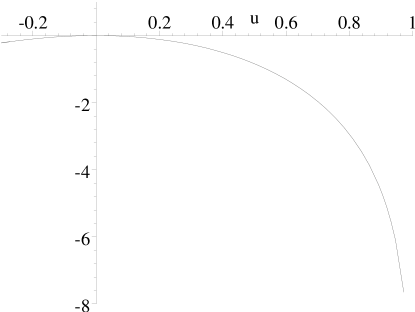
Figure 21: A plot of Eq. (92) with $8\pi^{2}/g^{2}N_{c}$ (along the vertical axis) against $u$.

As we can see in Fig. 21 this minimal choice shows no physical eigenvalue, since there is no positive solution for $8\pi^{2}/g^{2}N_{c}$ for any value of $u\in[0,1]$.

Finally, the $M\!=\!2$ color adjoint magnetic scalar propagator also receives self energy corrections which can be summed exactly (see Fig. 22). (Note that the fictitious electric scalar (solid line propagator) does not play a role in the $M\!=\!2$ channel, since it’s coupling to two $M\!=\!1$ transverse gluons is zero.) Although the magnetic scalar’s contribution to the dynamics of a color singlet $M\!=\!2$ glueball cancels, its propagator describes a spin 0 $M\!=\!2$ color adjoint subsystem in larger fishnets, and so it is also useful to analyze it here.

Figure 22: Magnetic scalar propagator for $M\!=\!2$. In each bubble the transverse gluon index may circulate in either direction.

In these diagrams the bubbles correspond to the one-loop self energy diagrams of the fictitious magnetic scalar (the dashed scalar).

Figure 23: The two bubble diagrams that contribute to the magnetic scalar self energy, $\Pi_{m}$.

The magnetic scalar self energy (see Fig. 23) is given by

$$\Pi_{m} = {g^{2}N_{c}\over 2T_{0}^{2}}\sum_{k=1}^{\infty}u^{k}\int{d^{2}{\bf p}\over(2\pi)^{3}}e^{-k{\bf p}^{2}/T_{0}}$$ (93)

$$= {g^{2}N_{c}\over 16\pi^{2}}{1\over T_{0}}\sum_{k=1}^{\infty}{u^{k}\over k}$$

$$= -{g^{2}N_{c}\over 16\pi^{2}}{1\over T_{0}}\ln(1-u).$$

The bare magnetic scalar propagator for $M\!=\!2$ is then

$$D_{m}=-T_{0}\sum_{k=1}^{\infty}h_{k}(2)\,u^{k},$$ (94)

where the $h_{k}(2)$ have to obey the constraints

$$\sum_{k=1}^{\infty}h_{k}(2)=1,\qquad\sum_{k=1}^{\infty}{h_{k}(2)\over k}=-{\pi^{2}\over 36}.$$ (95)

The exact propagator is then given by the geometric series

$${\tilde{D}}_{m} = D_{m}\sum_{l=0}^{\infty}\left(\Pi_{m}D_{m}\right)^{l}\>\,=\>\,{D_{m}\over 1-\Pi_{m}D_{m}}.$$ (96)

We again investigate possible energy eigenstates by looking at the pole structure of this amplitude. Focusing on the denominator we see

$${\tilde{D}}_{m} \propto \left[{8\pi^{2}\over g^{2}N_{c}}-{1\over 2}\left(\sum_{k=1}^{\infty}h_{k}(2)u^{k}\right)\ln(1-u)\right]^{-1}.$$ (97)

Again we see the same possible behaviors as in the case of the gluon propagator (except, of course, there is no massless pole at $u=1$!). In this case we also present the results of choosing a minimal set of the $h_{k}(2)$ to satisfy the constraints. Doing this yields

$$h_{1}(2)=-1-{\pi^{2}\over 18},\qquad h_{2}(2)=2+{\pi^{2}\over 18}.$$ (98)

With this set of parameters the denominator factor in (97) will have a pole if there is a solution to the following equation

$${8\pi^{2}\over g^{2}N_{c}} = {1\over 2}\left(h_{1}(2)u+h_{2}(2)u^{2}\right)\ln(1-u)$$ (99)

$$= -{1\over 2}\left|h_{1}(2)\right|u(1-|\alpha|u)\ln(1-u),$$

where $\alpha\equiv h_{2}(2)/h_{1}(2)\approx-1.646$.

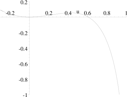
Figure 24: A plot of Eq. (99) with $8\pi^{2}/g^{2}N_{c}$ (along the vertical axis) against $u$.

As we can see in Fig. 24, this minimal choice shows a physical bound state (actually two) with $0<u<1$ for the coupling greater than some critical value, $g^{2}N_{c}/8\pi^{2}\gtrsim 18.28$. Such a bound state would be significant because it would mean that the short-lived magnetic scalar, which we have introduced as a device, can gain longevity at strong coupling, so that it can play the role of a spin 0 gluon in larger diagrams.

There is also a solution for negative $u$ for all couplings. From the interpretation $u=e^{aE}$ we see that these solutions would correspond to complex energies with imaginary part $\pm\pi i/a$. In fact the relation between $u$ and $E$ is fundamentally ambiguous by the imaginary amount $2\pi in/a$ simply due to the discretization of $\tau$. We presume that this ambiguity is simply a lattice artifact, and it seems likely that the solutions with negative $u$ are also artifacts. However, the ultimate proof of their artifactual nature must await a more complete understanding of the continuum limit, which will involve taking $M\to\infty$ as well as $a\to 0$.

5.2 Strong Coupling $M\!=\!4$ Scalar Fishnet

Clearly we need to be able to deal with large values of $M$ if we are to understand QCD. In this section, to better understand what this will involve, we look more closely at the $M\!=\!4$ sector of the simpler paradigm scalar theory. In particular we would like to explore the effect of the $\kappa^{2}$-term on the l.h.s. of the strong coupling Eq. (61). Recall that we have set $1-\delta_{1}=\kappa^{2}$. We dropped this term in the analysis of Sec. 4 because it made the equation intractable for general $n$. However, for the special case of $M\!=\!4$ ($n\equiv M/2=2$) it is possible to solve this equation. We also note that this case was not covered in Sec. 4 (even with the $\kappa^{2}$-term removed) because of the limitation to odd $n$. The additional special case of $M\!=\!6$ will be investigated in the following subsection.

For $M\!=\!4$ the strong coupling eigenvalue equation reads

$$\hskip-28.45274pt\left(t^{2}-\kappa^{2}\lambda^{2}e^{-({\bf q}_{1}^{2}+{\bf q}_{2}^{2})/2T_{0}}\right)\psi_{2}({\bf q}_{1},{\bf q}_{2}) =$$ (100)

$$\hskip-142.26378pt\lambda^{2}e^{-({\bf q}_{1}^{2}+{\bf q}_{2}^{2})/2T_{0}}\int{d^{2}k_{1}\over\pi T_{0}}{d^{2}k_{2}\over\pi T_{0}}\psi_{2}({\bf q}_{T}/2+{\bf k}_{2}-{\bf k}_{1},{\bf q}_{T}/2+{\bf k}_{1}-{\bf k}_{2})e^{-({\bf k}_{1}^{2}+{\bf k}_{2}^{2})/T_{0}},$$

where ${\bf q}_{T}={\bf q}_{1}+{\bf q}_{2}$. After the change of variables (${\bf k}_{T}\equiv{\bf k}_{1}+{\bf k}_{2}$ and ${\bf k}\equiv{\bf k}_{2}-{\bf k}_{1}$) we can integrate with respect to ${\bf k}_{T}$ on the r.h.s. What remains is

$$\hskip-28.45274pt\left(t^{2}-\kappa^{2}\lambda^{2}e^{-({\bf q}_{1}^{2}+{\bf q}_{2}^{2})/2T_{0}}\right)\psi_{2}({\bf q}_{1},{\bf q}_{2}) =$$ (101)

$$\hskip-142.26378pt{\lambda^{2}\over 2}e^{-({\bf q}_{1}^{2}+{\bf q}_{2}^{2})/2T_{0}}\int{d^{2}k\over\pi T_{0}}\psi_{2}({\bf q}_{T}/2+{\bf k},{\bf q}_{T}/2-{\bf k})e^{-{\bf k}^{2}/2T_{0}}.$$

If we now perform a variable transformation on the ${\bf q}$’s (${\bf q}_{T}\equiv{\bf q}_{1}+{\bf q}_{2}$ and ${\bf q}\equiv({\bf q}_{1}-{\bf q}_{2})/2$) then the equation becomes

$$\hskip-28.45274pt\left(t^{2}-\kappa^{2}\lambda^{2}e^{-({\bf q}_{T}^{2}+4{\bf q}^{2})/4T_{0}}\right)\psi_{2}({\bf q}_{T}/2+{\bf q},{\bf q}_{T}/2-{\bf q}) =$$ (102)

$$\hskip-142.26378pt{\lambda^{2}\over 2}e^{-({\bf q}_{T}^{2}+4{\bf q}^{2})/4T_{0}}\int{d^{2}k\over\pi T_{0}}\psi_{2}({\bf q}_{T}/2+{\bf k},{\bf q}_{T}/2-{\bf k})e^{-{\bf k}^{2}/2T_{0}}.$$

We can absorb the ${\bf q}_{T}$ dependence by scaling $t=t_{0}\exp(-{\bf q}_{T}^{2}/8T_{0})$, in effect going to the center of mass frame.

For the case of ${t}_{0}^{2}>\kappa^{2}\lambda^{2}$, we can eliminate the $\psi_{2}$ dependence by manipulating this equation and integrating with respect to ${d^{2}q}$. The result

$$1={\lambda^{2}\over 2}\int{d^{2}q\over\pi T_{0}}{e^{-3{\bf q}^{2}/2T_{0}}\over t_{0}^{2}-\kappa^{2}\lambda^{2}e^{-{\bf q}^{2}/T_{0}}},$$ (103)

is a transcendental equation for the eigenvalue, as is readily seen by direct evaluation of the integral:

$$\kappa^{2}={\hat{t}\over 2\kappa}\ln{\hat{t}+\kappa\over\hat{t}-\kappa}-1,$$ (104)

where $\hat{t}\equiv t_{0}/\lambda$ and we have assumed $\kappa^{2}>0$. If $\kappa^{2}<0$ we write $\kappa\equiv i\alpha$ and the equation becomes

$$1-\alpha^{2}={\hat{t}\over\alpha}\tan^{-1}\left({\alpha\over{\hat{t}}}\right).$$ (105)

It is immediately clear that a solution exists in this case only for $\alpha^{2}=-\kappa^{2}<1$.

If we analyze (104) we see that by varying $\hat{t}$ between $\kappa$ and $\infty$ the r.h.s. takes on values between $0$ and $\infty$, thus there is a solution to this equation for any value of $\kappa$. For the special case of $\kappa=0$, a more careful analysis of this equation also yields a solution. For a given eigenvalue solution to (104) the eigenfunction is given by

$$\psi_{2}({\bf q})={e^{-{\bf q}^{2}/T_{0}}\over 2\left({\hat{t}}^{2}-\kappa^{2}e^{-{\bf q}^{2}/T_{0}}\right)}\int{d^{2}k\over\pi T_{0}}\psi_{2}({\bf k})e^{-{\bf k}^{2}/2T_{0}},$$ (106)

where the integral on the r.h.s. represents a number that can be fixed by normalization.

If we refer back to (102) we see that if $\hat{t}^{2}<\kappa^{2}$, then a delta function term restricting momentum to energy shell may be added. For $s$-waves (non $s$-waves are free), we then have

$$\psi_{2}({\bf q})=A\delta\!\left({\bf q}^{2}-T_{0}\ln{\kappa^{2}\over\hat{t}^{2}}\right)+{e^{-{\bf q}^{2}/T_{0}}\over 2\left({\hat{t}}^{2}-\kappa^{2}e^{-{\bf q}^{2}/T_{0}}+i\epsilon\right)}\int{d^{2}k\over\pi T_{0}}\psi_{2}({\bf k})e^{-{\bf k}^{2}/2T_{0}},$$ (107)

where the coefficient of the delta function can be fixed via the following equation which relates $A$ to the normalization of the wavefunction,

$$\int{d^{2}q\over\pi T_{0}}\psi_{2}({\bf q})e^{-{\bf q}^{2}/2T_{0}}={A\over T_{0}}\left|{\hat{t}\over\kappa}\right|+\int{d^{2}q\over\pi T_{0}}{e^{-3{\bf q}^{2}/2T_{0}}\over 2\left({\hat{t}}^{2}-\kappa^{2}e^{-{\bf q}^{2}/T_{0}}+i\epsilon\right)}\int{d^{2}k\over\pi T_{0}}\psi_{2}({\bf k})e^{-{\bf k}^{2}/2T_{0}}.$$ (108)

In this case, $\hat{t}^{2}<\kappa^{2}$, there is no restriction on the value of $\hat{t}$, thus this solution corresponds to the continuum. To summarize the spectrum of $t_{0}^{2}$ includes a discrete $s$-wave bound state and a continuum for $t_{0}^{2}<\kappa^{2}\lambda^{2}$. Clearly the discrete state will not change drastically in the limit $\kappa\to 0$, but the continuum would be dramatically squeezed to a set of measure zero in this limit.

5.3 Strong Coupling $M\!=\!6$ Scalar Fishnet

The starting point for evaluating the strong coupling $M\!=\!6$ bit scalar fishnet diagrams is Eq. (61). For $n=M/2=3$ the equation to solve is

$$\hskip-28.45274pt\left(t^{2}-\kappa^{2}\lambda^{3}e^{-({\bf q}_{1}^{2}+{\bf q}_{2}^{2}+{\bf q}_{3}^{2})/2T_{0}}\right)\psi_{3}({\bf q}_{1},{\bf q}_{2},{\bf q}_{3}) = \lambda^{3}e^{-({\bf q}_{1}^{2}+{\bf q}_{2}^{2}+{\bf q}_{3}^{2})/2T_{0}}\int{d^{2}k_{1}\over\pi T_{0}}{d^{2}k_{2}\over\pi T_{0}}{d^{2}k_{3}\over\pi T_{0}}$$ (109)

$$\hskip-156.49014pt\psi_{3}(({\bf q}_{1}+{\bf q}_{2})/2+{\bf k}_{21},({\bf q}_{2}+{\bf q}_{3})/2+{\bf k}_{32},({\bf q}_{3}+{\bf q}_{1})/2+{\bf k}_{13})e^{-({\bf k}_{1}^{2}+{\bf k}_{2}^{2}+{\bf k}_{3}^{2})/T_{0}},$$

where we have used ${\bf k}_{ij}={\bf k}_{i}-{\bf k}_{j}$. By working in the center of mass frame, we can replace ${\bf q}_{3}\rightarrow-{\bf q}_{1}-{\bf q}_{2}$ and the equation becomes

$$\hskip-28.45274pt\left(t^{2}-\kappa^{2}\lambda^{3}e^{-({\bf q}_{1}^{2}+{\bf q}_{2}^{2}+{\bf q}_{1}\cdot{\bf q}_{2})/T_{0}}\right)\psi_{3}({\bf q}_{1},{\bf q}_{2},-{\bf q}_{1}-{\bf q}_{2}) = \lambda^{3}e^{-({\bf q}_{1}^{2}+{\bf q}_{2}^{2}+{\bf q}_{1}\cdot{\bf q}_{2})/T_{0}}\int{d^{2}k_{1}\over\pi T_{0}}{d^{2}k_{2}\over\pi T_{0}}{d^{2}k_{3}\over\pi T_{0}}$$ (110)

$$\hskip-142.26378pt\psi_{3}({\bf q}_{1}/2+{\bf q}_{2}/2+{\bf k}_{21},-{\bf q}_{1}/2+{\bf k}_{32},-{\bf q}_{2}/2+{\bf k}_{13})e^{-({\bf k}_{1}^{2}+{\bf k}_{2}^{2}+{\bf k}_{3}^{2})/T_{0}}.$$

If we change the integration variables ${\bf k}_{2}$ and ${\bf k}_{3}$ on the r.h.s. to

$${\bf p}_{1}={\bf q}_{1}/2+{\bf q}_{2}/2+{\bf k}_{21},\qquad{\bf p}_{2}=-{\bf q}_{1}/2+{\bf k}_{32},$$ (111)

then we see that $\psi_{3}$ in the integrand on the r.h.s. is independent of ${\bf k}_{1}$, so the Gaussian integral over ${\bf k}_{1}$ may be trivially performed by completing the square.

Once this has been done the result is

$$\hskip-28.45274pt\left(t^{2}-\kappa^{2}\lambda^{3}e^{-({\bf q}_{1}^{2}+{\bf q}_{2}^{2}+{\bf q}_{1}\cdot{\bf q}_{2})/T_{0}}\right)\psi_{3}({\bf q}_{1},{\bf q}_{2}) = {\lambda^{3}\over 3}e^{-({\bf q}_{1}^{2}+{\bf q}_{2}^{2}+{\bf q}_{1}\cdot{\bf q}_{2})/T_{0}}\int{d^{2}p_{1}\over\pi T_{0}}{d^{2}p_{2}\over\pi T_{0}}\psi_{3}({\bf p}_{1},{\bf p}_{2})$$ (112)

$$\hskip-71.13188pt\times\exp\left[-{2\over 3T_{0}}\left({\bf p}_{1}^{2}+{\bf p}_{2}^{2}+{\bf p}_{1}\cdot{\bf p}_{2}\right)-{1\over 6T_{0}}\left({\bf q}_{1}^{2}+{\bf q}_{2}^{2}+{\bf q}_{1}\cdot{\bf q}_{2}\right)\right.$$

$$\hskip-71.13188pt\phantom{\times\exp\left[\right.}\left.+{1\over 3T_{0}}\left({\bf p}_{1}\cdot{\bf q}_{1}+2{\bf p}_{1}\cdot{\bf q}_{2}-{\bf p}_{2}\cdot{\bf q}_{1}+{\bf p}_{2}\cdot{\bf q}_{2}\right)\right].$$

In this equation we see that except for the last term in the exponential on the r.h.s. this integral equation only depends on the scalar quantity, ${\bf q}_{1}^{2}+{\bf q}_{2}^{2}+{\bf q}_{1}\cdot{\bf q}_{2}$. This is not surprising since this scalar quantity is proportional to ${\bf q}_{1}^{2}+{\bf q}_{2}^{2}+{\bf q}_{3}^{2}$ and is the only cyclically invariant (${\bf q}_{i}\rightarrow{\bf q}_{i+1}$) scalar of order ${\bf q}^{2}$. We next perform another change of variables,

$${{\bf q}_{1}\over\sqrt{T_{0}}}={\bf u}_{1}+{\bf u}_{2},\qquad{{\bf q}_{2}\over\sqrt{T_{0}}}={\bf u}_{1}-{\bf u}_{2},\qquad{{\bf p}_{1}\over\sqrt{T_{0}}}={\bf v}_{1}+{\bf v}_{2},\qquad{{\bf p}_{2}\over\sqrt{T_{0}}}={\bf v}_{1}-{\bf v}_{2},$$ (113)

remembering that ${\bf q}_{i}$, ${\bf p}_{i}$ and now ${\bf u}_{i}$, ${\bf v}_{i}$ are Euclidean 2-vectors. With these substitutions our equation becomes

$$\hskip-28.45274pt\left(t^{2}-\kappa^{2}\lambda^{3}e^{-(3{\bf u}_{1}^{2}+{\bf u}_{2}^{2})}\right)\psi_{3}({\bf u}_{1},{\bf u}_{2}) = {4\lambda^{3}\over 3\pi^{2}}e^{-(3{\bf u}_{1}^{2}+{\bf u}_{2}^{2})}\int{d^{2}v_{1}}{d^{2}v_{2}}\,\psi_{3}({\bf v}_{1},{\bf v}_{2})$$ (114)

$$\hskip-170.71652pt\times\exp\left[-{2\over 3}\left(3{\bf v}_{1}^{2}+{\bf v}_{2}^{2}\right)-{1\over 6}\left(3{\bf u}_{1}^{2}+{\bf u}_{2}^{2}\right)+{\bf u}_{1}\cdot{\bf v}_{1}+{\bf u}_{1}\cdot{\bf v}_{2}-{\bf u}_{2}\cdot{\bf v}_{1}+{1\over 3}{\bf u}_{2}\cdot{\bf v}_{2}\right].$$

If we rescale ${\bf u}_{2}$ and ${\bf v}_{2}$ by a factor of $\sqrt{3}$, then we can make the $O(4)$ symmetry manifest (up to the last four terms in the exponential on the r.h.s.) by combining ${\bf u}_{1}$ and ${\bf u}_{2}$ (${\bf v}_{1}$ and ${\bf v}_{2}$) into a Euclidean 4-vector ${\bf U}$ (${\bf V}$). Thus the equation may be written as

$$\left(t^{2}-\kappa^{2}\lambda^{3}e^{-3{\bf U}^{2}}\right)\psi_{3}({\bf U}) = {4\lambda^{3}\over\pi^{2}}e^{-7{\bf U}^{2}/2}\int{d^{4}V}\,\psi_{3}({\bf V})e^{-2{\bf V}^{2}+2{\bf V}^{\rm T}\mbox{${\cal R}$}{\bf U}},$$ (115)

$$= {4\lambda^{3}\over\pi^{2}}e^{-7{\bf U}^{2}/2}\int{d^{4}V}\,\psi_{3}(\mbox{${\cal R}$}{\bf V})e^{-2{\bf V}^{2}+2{\bf V}\cdot{\bf U}},$$

where ${\cal R}$ is the real orthogonal $O(4)$ rotation:

$$\mbox{${\cal R}$}\equiv{1\over 2}\left(\begin{array}[]{cccc}1&0&-\sqrt{3}&0\\ 0&1&0&-\sqrt{3}\\ \sqrt{3}&0&1&0\\ 0&\sqrt{3}&0&1\\ \end{array}\right).$$ (116)

We note that ${\cal R}^{3}=-1$. We can search for an $O(4)$ invariant solution to this equation which is a function only of the length, $\|{\bf U}\|$. Although this will not yield the most general eigenstate, it is expected to include the ground state. Plugging in this ansatz, the equation simplifies to

$$\left(t^{2}-\kappa^{2}\lambda^{3}e^{-3U^{2}}\right)\psi_{3}(U) = {4\lambda^{3}\over\pi^{2}}e^{-7U^{2}/2}\int{V^{3}dV}\,\psi_{3}(V)e^{-2V^{2}}\int{d\Omega_{\bf V}}e^{2{\bf V}\cdot{\bf U}},$$ (117)

where $U\equiv\|{\bf U}\|$ and $V\equiv\|{\bf V}\|$. The angular integral on the r.h.s. may be evaluated with standard techniques,

$$\int{d\Omega_{\bf V}}e^{2{\bf V}\cdot{\bf U}} = 4\pi\int_{-1}^{1}d\zeta\sqrt{1-\zeta^{2}}e^{2UV\zeta}$$ (118)

$$= {2\pi^{2}I_{1}(2UV)\over UV},$$

where $I_{1}(x)$ is the modified Bessel function regular at $x=0$.

Thus the integral equation to solve is

$$t^{2}\psi_{3}(U) = \kappa^{2}\lambda^{3}e^{-3U^{2}}\psi_{3}(U)+{8\lambda^{3}}{e^{-7U^{2}/2}\over U}\int{V^{2}dV}\,I_{1}(2UV)\psi_{3}(V)e^{-2V^{2}}.$$ (119)

The first thing to note is that for $\kappa^{2}=0$ the eigenfunction solution is a Gaussian of the form

$$\psi_{3}(U)=e^{-\xi U^{2}},\qquad\mbox{where}\qquad\xi={3+\sqrt{105}\over 4}.$$ (120)

For this solution the corresponding eigenvalue is

$$t^{2}={64\lambda^{3}\over\left(11+\sqrt{105}\right)^{2}}.$$ (121)

Both of these match the values predicted by Equations (76) and (81) for $n=3$. For $\kappa^{2}$ away from zero we can solve this integral equation by means of an iterative procedure. Starting with the solution for $\kappa^{2}=0$ we can iterate the r.h.s. of (119) repeatedly. This is a convenient way of solving this equation since the functions generated by the integral on the r.h.s. are always Gaussian. Thus at each iteration step the solution will be of the form

$$\psi_{3}(U)=\sum_{n}c_{n}e^{-\alpha_{n}U^{2}},$$ (122)

with the number of terms in the sum doubling after each iteration. For a solution of this form it can be shown that the corresponding eigenvalue, $t^{2}$, is given by

$$t^{2}=\kappa^{2}+{4\sum_{n}c_{n}/(2+\alpha_{n})^{2}\over\sum_{n}c_{n}}.$$ (123)

We have tested this iteration procedure numerically and for values of $\kappa^{2}$ small ($\kappa^{2}<0.3$) we see that the wavefunction(eigenvalue) converges to a well-defined function(value). For $\kappa^{2}$ larger (closer to 1) this becomes murkier as one needs a lot more iterations for the convergence to a value distinct from $\kappa^{2}$ to be evident. Another interesting phenomenon is that for $\kappa^{2}\lesssim-0.11$, then $t^{2}$ becomes negative indicating that no physical solution exists.

6 Conclusion

In this article, we have refined and extended an approach, proposed in the late seventies, to obtain the large $N_{c}$ limit of QCD by directly summing the planar diagrams which survive. The basic tool is to define the planar diagrams using light-front space-time coordinates for which $ix^{+}$ and the $p^{+}$ carried by each gluon are discretized. This effectively digitizes the sum of diagrams, a first step toward a numerical evaluation. It also regulates the usual divergences of Feynman diagrams. We identified several shortcomings of the discretized model of QCD attempted in [5], and we proposed an improved formulation which at least mitigates, and might well overcome, these defects.

Discretization enables a formal strong ’t Hooft coupling limit of the sum of diagrams. A major disadvantage of the discretization of [5] was that this formal limit suppressed the cubic gluonic interaction essential for the “anti-ferromagnetic” ordering of glueball mass levels: the dominant quartic interaction ordered levels ferromagnetically. Our new discretized model replaces the quartic interactions by the exchange of two kinds of fictitious “short-lived” scalars, so that all interactions can compete on an equal footing in the strong coupling limit. The ambiguities inherent in such a replacement can also be exploited to remove unwanted symmetry violations induced by the usual ultraviolet divergences present in the continuum limit.

Having defined our discretized model, we explored its physical properties in several ways. We first studied the nature of weak coupling perturbation theory by calculating the gluon self energy to one loop order, regaining the known continuum answer. This calculation showed how the discretization regulates ultraviolet divergences, and how the ambiguities in the model begin to be fixed by the restoration of Poincaré invariance. Although we have not done a two loop calculation, there is sufficient flexibility in these ambiguities to hope to achieve Poincaré invariance to all orders in perturbation theory. The discretized model can also be studied in the strong coupling limit, but in this article we just began this study for QCD by looking only at states with very small total $P^{+}=Mm$ for $M\!=\!2$, where the dynamics is so drastically simplified that it can be solved exactly. We defer to a future publication studies of QCD at $M\!=\!3$ and higher. The continuum limit, of course, will require $M\to\infty$.

As a warmup for going to larger values of $M$, we evaluated the strong coupling limit in a paradigm matrix scalar field theory with only cubic interactions. Not surprisingly, the bosonic light-cone string was obtained. Although this paradigm model yielded some useful insights into the nature of large planar diagrams, we stressed that the corresponding QCD calculation will have profound differences: for one thing the gluons carry spin, and for another their interactions show both repulsion and attraction depending on the quantum numbers of the channel. In contrast, the interactions of the scalar theory are exclusively attractive. Because of this, the strong coupling limit forced the $p^{+}$ carried by each scalar quantum to be minimal, i.e. one discretized unit $m$. This circumstance prevented a “Liouville” degree of freedom, associated with collective fluctuations of the $P^{+}$ distribution among the scalar quanta, from arising. Thus the limit must be interpreted as a critical string theory.

The diversity of interaction signs of QCD will obviously complicate this outcome. It is possible, and a major focus for future study, that cancellations deemphasize the contributions where all quanta carry the minimum $p^{+}$ to such a degree that a collective Liouville field emerges. Then the strong coupling limit might be a subcritical version of one of the existing string models. If so, the Liouville world-sheet field could be thought of as a fifth dimension, and the dual description of our model as a field theory at weak coupling and a subcritical string theory at strong coupling would resemble the anti de Sitter gravity (AdS) / conformal field theory (CFT) duality of [17, 2, 18]. Another logical possibility, though, is that the strong coupling limit of large $N_{c}$ QCD is actually a novel critical string theory with critical dimension 4. Of course, it could also turn out that the attempt to reach a reasonable Poincaré invariant strong coupling limit of large $N_{c}$ QCD simply fails. After all, continuum QCD is, strictly speaking, not an infinite coupling theory in any sense of the word. The coupling is scale dependent and corresponds to no tunable parameter at all. The strong coupling limit, as everyone knows, describes the discretized model and can vary wildly from one discretization to another.

Much has been said about the “holographic” nature of the duality mentioned above. We would like to conclude with a few comments about this. The hologram metaphor was invented by ’t Hooft [19] to describe a possible resolution of the “information loss paradox” of quantum black holes. Since the horizon of a black hole is two dimensional, it should be possible to describe all of three dimensional physics by a two dimensional quantum theory. The discretized model we have presented here is not holographic in this sense. The transverse space of a light front is indeed two dimensional, but the third longitudinal dimension has not been eliminated: it is present in the disguised form of a variable Newtonian mass $Mm$ for each gluon. However, the model is holographic in the higher dimensional sense described by Witten [18]. The “fundamental” discretized model is $3+1$ dimensional, 2 transverse dimensions, variable $p^{+}$ and $x^{+}$. However in the strong coupling limit we expect $4+1$ dimensions: the $x^{-}$ of light-cone string should emerge as a function of the transverse and Liouville degrees of freedom. Holography in ’t Hooft’s sense would require a more profound circumstance: there should be no Liouville field and the variable $p^{+}$ of each gluon must itself be a mere collective effect. For example, the gluon with $M$ units of $p^{+}$ might be thought of as a bound system of $M$ minimal $p^{+}$ “bits” [20]. In that case, the model presented here would just be a stepping stone toward that more fundamental theory.

Acknowledgments: We would like to thank M. Brisudova for helpful criticism of the manuscript. JSR and CBT would also like to acknowledge the Aspen Center for Physics where part of this work was completed. This work was supported in part by the Department of Energy under Grant No. DE-FG02-97ER-41029.

A Appendix: Alternate Discretization

In this appendix we explore the ramifications of the alternate discretization Eq. (8) of $D^{--}$. The bare propagator in energy representation is

$${\tilde{D}}_{0}^{--}({\bf Q},M,E) = {T_{0}(e^{aE}-1)\over M^{2}}{u\over 1-u}.$$ (A.1)

The self-energy parts $\Pi^{kl},\Pi^{k+}$ and $\Pi^{++}$ will of course have different values in this discretization, but the decompositions (14) remain valid. Under the assumption that $\Pi^{\prime\prime}_{1}=\Pi^{\prime}_{1}=\Pi_{1}$, the relations of the exact propagators to the $\Pi$’s are identical to (15) except for ${\tilde{D}}^{--}$ for which the relation is

$${\tilde{D}}^{--} = {T_{0}\over M^{2}}\left[{u(e^{aE}-1-{\bf Q}^{2}/2MT_{0})\over 1-u-T_{0}u\Pi_{1}(e^{aE}-1-{\bf Q}^{2}/2MT_{0})}+{{\bf Q}^{2}\over 2MT_{0}}{u\over 1-u-u\Pi_{2I}/2M}\right].$$ (A.2)

The only parts of the one loop self energy calculation affected by the different discretization are the two diagrams, Fig. 12, which have a $D^{--}$ propagator as one of the internal lines. The evaluation is quite different for this discretization because the completion of squares in the second term of Eq. (8) leads to different factors than the first term. The contribution of the first term involves the exponent

$${k\over 2T_{0}}\left({{\bf p}^{2}\over l}+{({\bf Q}-{\bf p})^{2}\over M-l}\right)={k\over 2T_{0}}\left({M({\bf p}-l{\bf Q}/M)^{2}\over l(M-l)}{}+{{\bf Q}^{2}\over M}\right),$$ (A.3)

whereas the contribution of the second term involves

$${(k-1){\bf p}^{2}\over 2T_{0}l}+{k({\bf Q}-{\bf p})^{2}\over 2T_{0}(M-l)}={1\over 2T_{0}}\left({M(k-1)+l\over l(M-l)}{\left({\bf p}-{lk{\bf Q}\over M(k-1)+l}\right)^{2}}+{k(k-1){\bf Q}^{2}\over M(k-1)+l}\right),$$ (A.4)

for one of the two diagrams, and for the other a similar expression with ${\bf p}\to{\bf Q}-{\bf p}$ and $l\to M-l$. Thus the two contribute equally to $\Pi^{\wedge\vee}_{{\rm D}I}$:

$$\Pi^{\wedge\vee}_{{\rm D}} = {g^{2}N_{c}\over 4\pi^{2}}\sum_{l=1}^{M-1}{(2M-l)^{2}\over l}e^{-k{\bf Q}^{2}/2MT_{0}}\left[{e^{kl{\bf Q}^{2}/2MT_{0}(M(k-1)+l)}\over M(k-1)+l}-{1\over Mk}\right],$$ (A.5)

for $k>1$ and by

$$\Pi^{\wedge\vee}_{{\rm D}} = -{g^{2}N_{c}\over 4\pi^{2}}\sum_{l=1}^{M-1}{(2M-l)^{2}\over l}{e^{-{\bf Q}^{2}/2MT_{0}}\over M},$$ (A.6)

for $k=1$. Translating to energy representation gives the more compact

$${\tilde{\Pi}}^{\wedge\vee}_{\rm D} = {g^{2}N_{c}\over 4\pi^{2}}\sum_{l=1}^{M-1}{(2M-l)^{2}\over l}\sum_{k=1}^{\infty}u^{k}\left[u{e^{l(k+1){\bf Q}^{2}/2MT_{0}(Mk+l)}\over Mk+l}-{1\over Mk}\right].$$ (A.7)

Adding the result of the unchanged first thirteen diagrams to this and subtracting ${\bf Q}^{2}\Pi_{1}/2$ gives $\Pi_{2}$ for this discretization:

$${\Pi}_{2} = {g^{2}N_{c}\over 24\pi^{2}}{13M^{2}-12M-1\over M}\sum_{k=1}^{\infty}{u^{k}\over k^{2}}+{g^{2}N_{c}\over 48\pi^{2}}\left(14-{15\over M}+{1\over M^{2}}\right){{\bf Q}^{2}\over T_{0}}\ln(1-u)$$ (A.8)

$$\qquad+{g^{2}N_{c}\over 4\pi^{2}}\sum_{l=1}^{M-1}{(2M-l)^{2}\over l}\sum_{k=1}^{\infty}u^{k}\left[u{e^{l(k+1){\bf Q}^{2}/2MT_{0}(Mk+l)}\over Mk+l}-{1\over Mk}\right].$$

The violation of Galilei invariance caused by this alternate discretization is apparent from the non-polynomial dependence on ${\bf Q}^{2}$. However, one can easily see that each power of ${\bf Q}^{2}$ comes with an accompanying power of $1/M$. At most one power of $M$ is supplied by the prefactors, so all powers of ${\bf Q}^{2}$ higher than the first are irrelevant in the continuum limit.

In order to compare our results to the continuum calculation of Ref. [8], we must examine the limits $u\to 1$ and $M\to\infty$. The behavior of the first two terms of Eq. (A.8) in this limit is transparent once we use the identity (40). The continuum limit of the last term requires a bit more analysis. First, as mentioned in the previous paragraph, we only need keep two terms in the expansion of the exponential:

$${g^{2}N_{c}\over 4\pi^{2}}\left\{\sum_{l=1}^{M-1}{(2M-l)^{2}\over l}\sum_{k=1}^{\infty}u^{k}\left[{u\over Mk+l}-{1\over Mk}\right]+{{\bf Q}^{2}\over 2T_{0}}\sum_{l=1}^{M-1}{(2M-l)^{2}\over M^{3}}\sum_{k=1}^{\infty}{u^{k+1}(k+1)\over(k+l/M)^{2}}\right\}.$$ (A.9)

The sums over $l$ can be approximated using the Euler-Maclaurin summation formula, see Eq. (83), as long as $F$ is not singular at the endpoints of integration. Clearly terms with $1/l$ in the summand must be treated separately, which is easily handled using (35). Applying these formulae, we find (for large $M$ but arbitrary $u$),

$$\hskip-36.135pt\sum_{l=1}^{M-1}{(2M-l)^{2}\over l}\sum_{k=1}^{\infty}u^{k}\left[{u\over Mk+l}-{1\over Mk}\right]$$ (A.10)

$$= -\sum_{k=1}^{\infty}{u^{k+1}\over k}\sum_{l=1}^{M-1}{(2-l/M)^{2}\over k+l/M}+4M(1-u)\ln(1-u)\left[\psi(M)+\gamma-{7\over 8}+{7\over 8M}\right]$$

$$\sim -\sum_{k=1}^{\infty}{u^{k+1}\over k}M\left[{7\over 3k}+(k+2)^{2}\left(\ln\left(1+{1\over k}\right)-{1\over k}+{1\over 2k^{2}}\right)-{1\over 3k}-{2\over k^{2}}-{1\over 2M}\left({4\over k}+{1\over k+1}\right)\right]$$

$$\mbox{}+4M\left[\ln M+\gamma-{7\over 8}\right](1-u)\ln(1-u)$$

$$\hskip-36.135pt{{\bf Q}^{2}\over 2T_{0}}\sum_{l=1}^{M-1}{(2M-l)^{2}\over M^{3}}\sum_{k=1}^{\infty}{u^{k+1}(k+1)\over(k+l/M)^{2}}$$

$$\sim {{\bf Q}^{2}\over 2T_{0}}\sum_{k=1}^{\infty}u^{k+1}\left[{7\over 3k}-{4\over 3k^{3}}-2(k+1)(k+2)\left\{\ln\left(1+{1\over k}\right)-{1\over k}+{1\over 2k^{2}}-{1\over 3k^{3}}\right\}\right]$$

The continuum limit also requires $1-u\sim Q^{2}/2MT_{0}=({\bf Q}^{2}-2mME)/2MT_{0}$, so $u$ may be set to unity in all nonsingular terms without a prefactor of $M$. Then the above terms simplify to

$$\hskip-36.135pt\sum_{l=1}^{M-1}{(2M-l)^{2}\over l}\sum_{k=1}^{\infty}u^{k}\left[{u\over Mk+l}-{1\over Mk}\right]$$ (A.11)

$$\sim \left({\alpha\over 6}-{\pi^{2}\over 3}\right)M+{\pi^{2}\over 3}+{1\over 2}+{Q^{2}\over 2T_{0}}\left(\beta+{7\over 3}\right)+{2Q^{2}\over T_{0}}\left(\ln M+\gamma-{35\over 24}\right)\ln(1-u)$$

$$\hskip-36.135pt{{\bf Q}^{2}\over 2T_{0}}\sum_{l=1}^{M-1}{(2M-l)^{2}\over M^{3}}\sum_{k=1}^{\infty}{u^{k+1}(k+1)\over(k+l/M)^{2}}\sim{{\bf Q}^{2}\over 2T_{0}}\left[-{7\over 3}\ln(1-u)+\delta\right]$$

where we have defined

$$\alpha = 12\zeta(3)-6\sum_{k=1}^{\infty}{(k+2)^{2}\over k}\left(\ln\left(1+{1\over k}\right)-{1\over k}+{1\over 2k^{2}}\right)$$ (A.12)

$$\beta = {7\pi^{2}\over 18}+\sum_{k=1}^{\infty}{k+1\over k}\left[(k+2)^{2}\left(\ln\left(1+{1\over k}\right)-{1\over k}+{1\over 2k^{2}}\right)-{1\over 3k}-{2\over k^{2}}\right]$$ (A.13)

$$\delta = -{4\over 3}\zeta(3)-2\sum_{k=1}^{\infty}(k+1)(k+2)\left[\ln\left(1+{1\over k}\right)-{1\over k}+{1\over 2k^{2}}-{1\over 3k^{3}}\right]$$ (A.14)

which can be numerical evaluated:

$$\alpha\approx 1.188,\qquad\beta\approx 1.991,\qquad\delta\approx 0.633.$$ (A.15)

Putting all this together, we get for the continuum limit,

$$\Pi_{2} = M{g^{2}N_{c}\over 24\pi^{2}}\left[\alpha+{\pi^{2}\over 6}\right]+{g^{2}N_{c}\over 4\pi^{2}}\left[{\pi^{2}\over 3}+{1\over 2}-{{\bf Q}^{2}\over T_{0}}{7\delta\over 6}\right]$$ (A.16)

$$\qquad+{g^{2}N_{c}\over 16\pi^{2}}{Q^{2}\over T_{0}}\left[8\ln M+8\gamma-{22\over 3}\right]\ln{Q^{2}\over 2MT_{0}}+{g^{2}N_{c}\over 24\pi^{2}}{Q^{2}\over 2T_{0}}[6\beta+1]$$

Remembering that our $\Pi_{2}$ is a factor of $-Q^{2}/T_{0}$ times that defined in Ref. [8], we find agreement for the coefficient of $\ln Q^{2}$, provided we identify $2MT_{0}$ with $\Lambda^{2}$. The first two groups of terms on the r.h.s. of Eq. (A.16) violate important symmetries and must be removed by explicit counter-terms. The term linear in ${\bf Q}^{2}$ violates Galilei invariance and the momentum independent terms imply a finite gluon mass squared in perturbation theory, thus violating Poincaré invariance. Note that the necessary counter terms are low order polynomials in both the transverse momentum and in the discretized $P^{+}$. Without the tadpole contributions the discretization used in the text would have required counter-terms with logarithmic $M$ dependence. But we found (at least at one-loop) that the tadpoles could be designed to eliminate the need for counter-terms. Then the fact that it preserves Galilei invariance makes it the superior choice.

References

- [1] G. ’t Hooft, Nucl. Phys. B72, 461 (1974).
- [2] S. S. Gubser, I. R. Klebanov, and A. M. Polyakov, Phys. Lett. B428, 105 (1998), hep-th/9802109.
-
[3]
H. B. Nielsen and P. Olesen, Phys. Lett. 32B, 203 (1970);
B. Sakita and M. A. Virasoro, Phys. Rev. Lett. 24, 1146 (1970). - [4] C. B. Thorn, Phys. Lett. 70B, 85 (1977); Phys. Rev. D 17, 1073 (1978).
- [5] R. Brower, R. Giles, and C. Thorn, Phys. Rev. D 18, 484 (1978).
-
[6]
J. B. Kogut and D. E. Soper, Phys. Rev. D 1, 2901 (1970);
E. Tomboulis, Phys. Rev. D 8, 2736 (1973). - [7] S. J. Brodsky, H-C. Pauli, and S. J. Pinsky, Phys. Rept. 301, 299 (1998), hep-ph/9705477.
- [8] C. B. Thorn, Phys. Rev. D 20, 1934 (1979).
- [9] E.H. Lieb and F.Y. Wu, in Phase Transitions and Critical Phenomena, edited by C. Domb and M.S. Green, (Academic, New York, 1972), P331.
- [10] C. B. Thorn, Phys. Rev. D 59, 116011 (1999), hep-th/9810066.
- [11] A. M. Polyakov, Phys. Lett. 103B, 207 (1981).
-
[12]
S. Dalley and I.R. Klebanov, Phys. Lett. B298, 79 (1993);
F. Antonuccio and S. Dalley, Phys. Lett. B348, 55 (1995). - [13] C. B. Thorn, Phys. Rev. D 20, 1435 (1979).
- [14] R. Giles and C. B. Thorn, Phys. Rev. D 16, 366 (1977).
- [15] J. S. Rozowsky and C. B. Thorn, Phys. Rev. D 60, 045001 (1999), hep-th/9902145.
- [16] L. Lewin, Polylogarithms and Associated Functions, (North Holland, Amsterdam, 1981).
- [17] J. M. Maldacena, Adv. Theor. Math. Phys. 2, 231 (1998), hep-th/9711200.
- [18] E. Witten, Adv. Theor. Math. Phys. 2, 253 (1998), hep-th/9802150.
- [19] G. ’t Hooft, “Dimensional Reduction in Quantum Gravity”, in Salamfestschrift, edited by A. Ali, J. Ellis and S. Randjbar-Daemi, (World Scientific, 1993), gr-qc/9310026.
- [20] C. B. Thorn, Phys. Rev. D 59, 025005 (1999), hep-th/9807151.