HUTP-99/A048

MIT-CTP-2903

hep-th/9909134

Modeling the fifth dimension
with scalars and gravity

O. DeWolfe,^1∗ D.Z. Freedman,^2∗ S.S. Gubser,^3∗ and A. Karch^1∗

¹ Center for Theoretical Physics, Massachusetts Institute of Technology, Cambridge, MA 02139-4307, USA ² Department of Mathematics and Center for Theoretical Physics, Massachusetts Institute of Technology, Cambridge, MA 02139-4307, USA ³ Lyman Laboratory of Physics, Harvard University, Cambridge, MA 02138, USA

Abstract

A method for obtaining solutions to the classical equations for scalars plus gravity in five dimensions is applied to some recent suggestions for brane-world phenomenology. The method involves only first order differential equations. It is inspired by gauged supergravity but does not require supersymmetry. Our first application is a full non-linear treatment of a recently studied stabilization mechanism for inter-brane spacing. The spacing is uniquely determined after conventional fine-tuning to achieve zero four-dimensional cosmological constant. If the fine-tuning is imperfect, there are solutions in which the four-dimensional branes are de Sitter or anti-de Sitter spacetimes. Our second application is a construction of smooth domain wall solutions which in a well-defined limit approach any desired array of sharply localized positive-tension branes. As an offshoot of the analysis we suggest a construction of a supergravity c-function for non-supersymmetric four-dimensional renormalization group flows.

The equations for fluctuations about an arbitrary scalar-gravity background are also studied. It is shown that all models in which the fifth dimension is effectively compactified contain a massless graviton. The graviton is the constant mode in the fifth dimension. The separated wave equation can be recast into the form of supersymmetric quantum mechanics. The graviton wave-function is then the supersymmetric ground state, and there are no tachyons.

September 1999

$\,{}^{*}$ odewolfe@ctp.mit.edu, dzf@math.mit.edu, ssgubser@born.harvard.edu, karch@mit.edu

1 Introduction

Phenomenologists have recently studied higher dimensional gravitational models containing one or more flat 3-branes embedded discontinuously in the ambient geometry. Scenarios with two 3-branes provide an explanation of the large hierarchy between the scales of weak and gravitational forces and contain a massless $2^{++}$ mode which reproduces Newtonian gravity at long range on the branes [1, 2]. In the following paper we present results of our study of models of this type: specifically, results on the smoothing of discontinuities and stabilization of inter-brane spacings in 5-dimensional models with gravity and a scalar field. The issue of fine-tuning in such models is also addressed. We also discuss the fluctuation equations in these models somewhat differently from treatments in the recent literature.

The centerpiece of this work is a supergravity-inspired approach to obtain exact solutions of the nonlinear classical field equations in gravity-scalar-brane models which is valid even without supersymmetry. After a brief introduction to the technical issues in section 2, this approach is presented in section 3 and applied to a class of models containing one positive and one negative tension brane [1] with compact $S_{1}/{\bf Z}_{2}$ geometry in the fifth dimension. Stabilization of the brane spacing is a generic feature of these models, but it is not guaranteed that the branes will be flat. Indeed, obtaining flat branes requires a fine-tuning of the model precisely equivalent to setting the four-dimensional cosmological constant to zero, and if the fine-tuning is imperfect, the induced metric on the branes will be de Sitter space or anti-de Sitter space. The stabilization mechanism is a generalization of the work of [3]; however, our treatment also includes back-reaction of the classical scalar profile. An explicit model is presented in section 4.

In section 5 we obtain smooth solutions of gravity-scalar models which approach discontinuous brane geometries in a certain “stiff limit.” Any array containing only positive tension branes can be smoothed in this way. We also remark on the usefulness of our first-order formalism for the description of supergravity duals to renormalization group flows.

Our constructions have some parallels in earlier supergravity domain wall literature (see [4] for a review). There are also similarities with more recent literature, for example [5, 6].

In section 6 we discuss the equations for linear fluctuations about a gravity-scalar-brane configuration. We use the axial gauge and a parameterization in which the 4-dimensional graviton appears universally as a constant mode in the fifth dimension. This mode is normalizable since that dimension is either manifestly or effectively compact. The graviton equation can be transformed into the form of a Schrödinger equation in supersymmetric quantum mechanics. The graviton is the supersymmetric ground state, so there is no lower energy state which would be a tachyon in the present context.

2 The issues

We start with the five-dimensional gravitational action

$$S=\int d^{5}x\,\sqrt{g}\left[-{1\over 4}R+{3\over L^{2}}\right]\,,$$ (1)

in $+----$ signature. The most general five-dimensional metric with four-dimensional Poincaré symmetry is

$$ds^{2}=e^{2A(r)}\,\eta_{ij}\,dx^{i}dx^{j}-dr^{2}\,,$$ (2)

with $\eta_{ij}=\mathop{\rm diag}\nolimits\{1,-1,-1,-1,-1\}$. Anti-de Sitter space is the solution of the field equations of (1) with $A(r)=-r/L$. This metric describes a Poincaré coordinate patch in $AdS_{5}$ with boundary region $r\rightarrow-\infty$ and Killing horizon region $r\rightarrow+\infty$.

The basic positive tension brane considered in [1, 2] is given by $A(r)=-|r|/L$. This can be thought of as the discontinuous (in first derivative) pasting of the horizon halves of two Poincaré patches with the 3-brane at $r=0$. One can obtain this as the solution of the field equations for an action consisting of (1) plus a brane tension term:

$$S_{brane}=-\sum_{\alpha}\int d^{4}x\,dr\,\sqrt{|\det g_{ij}|}\,\lambda_{\alpha}\,\delta(r-r_{\alpha})\,.$$ (3)

Here we have generalized to any number of branes; $g_{ij}$ is the metric induced on each brane by the ambient metric $g_{\mu\nu}$. For a single brane at $r_{1}=0$ with brane tension $\lambda_{1}$, the $AdS$ scale must be related by $1/L=\lambda_{1}/3$ to achieve a solution in which the induced metric is flat. This constraint represents a fine-tuning which is precisely equivalent to setting the four-dimensional cosmological constant equal to zero.

One can obtain a system of one positive and one negative tension brane [1] by considering two branes in (3) with $\lambda_{2}=-\lambda_{1}$ and $r_{2}=r_{0}$. This leads to the piece-wise linear scale function $A(r)$ shown in figure 1a. The fifth dimension is then periodic with period $2r_{0}$ and there is a reflection symmetry under $r\rightarrow-r$. This is the $S^{1}/{\bf Z}_{2}$ situation originally considered in [7, 8].

Figure 1: a) $A$ as a function of $r$ for the $S^{1}/{\bf Z}_{2}$ geometry, with one positive and one negative tension brane, each at a fixed point of ${\bf Z}_{2}$. b) $A$ as a function of $r$ for two positive tension branes in an infinite fifth dimension.

Another possibility is to consider [9] a second positive tension brane, which admits a solution for $A(r)$ shown in figure 1b. In this case, the bulk action (1) must be changed to admit different scales $L_{1}$, $L_{2}$, $L_{3}$ in the three spatial regions. The scales are related to the brane tensions by $1/L_{1}+1/L_{2}=2\lambda_{1}/3$ and $1/L_{3}-1/L_{2}=2\lambda_{2}/3>0$. Again these relations must be regarded as fine-tunings absent a dynamical mechanism by which they arise.

There are solutions of the equations of motion for any choice of the inter-brane spacing $r_{0}$ in both scenarios above, so it is important to ask whether there is any principle which fixes or stabilizes the value of $r_{0}$. A first thought is that the total action integral of the configuration might depend on $r_{0}$, reflecting an imbalance of forces on the two 3-branes, and therefore could be minimized. However it will be shown in the next section that the action vanishes for all $r_{0}$, which apparently reflects the fact that the “output” value of the classical four-dimensional cosmological constant vanishes, as is consistent with the “input” value assumed when we considered solutions containing flat 3-branes. In later sections we discuss models in which a real scalar field $\phi$ with potential $V(\phi)$ is coupled to gravity with brane tensions $\lambda_{\alpha}(\phi)$ depending on $\phi$. For a given choice of $V(\phi)$ and $\lambda_{\alpha}(\phi)$, it is generally the case that the brane spacing $r_{0}$ is uniquely determined.

Discontinuous solutions of field equations would be less artificial if they could be obtained as a limit of smooth configurations. In section 5 we present coupled scalar-gravity models with potential $V(\xi)$ (and no branes initially present). In these models the scalar $\xi$ plays a different role, that of an auxiliary field, and hence is given a different symbol. The models have smooth domain wall solutions which approach any desired discontinuous configuration of positive tension branes as a scale parameter in $V(\xi)$ is varied. Other parameters in $V(\xi)$ determine the inter-brane spacing (e.g. $r_{0}$) and $AdS$ scales (e.g. $L_{i}$) of the limiting solution, and the solutions have zero total action at all stages of the limiting procedure. The scalar $\xi$ is effectively frozen in the “stiff” limit of discontinuous branes.

Only positive tension brane configurations can be smoothed in this way. A negative tension brane effectively has negative energy which cannot be modeled in a conventional gravitational theory. Nevertheless a negative tension brane is consistent with micro-physical requirements if it is located at the fixed point of a discrete group action. The crucial point is that transverse fluctuations are then projected out; otherwise they would have negative kinetic terms.

3 The Goldberger-Wise mechanism

It was proposed in [3] that the dynamics of a scalar field could stabilize the size of an extra dimension in the brane-world scenario of [1]. The mechanism was to have a scalar $\phi$ with some mass in the bulk of a five-dimensional spacetime and some potentials $\lambda_{1}(\phi)$ and $\lambda_{2}(\phi)$ on two four-dimensional branes at the boundaries of this spacetime. Such a situation might be realized in the context of type I^′ string theory [10, 7], the Horava-Witten version of the heterotic string [8], or some more ornate string theory realization of the basic scenario of [1]: in all cases, spacetime has the topology ${\bf R}^{3,1}\times S^{1}/{\bf Z}_{2}$. The claim of [3] is that stabilization of the length of the interval $S^{1}/{\bf Z}_{2}$ can be achieved without fine-tuning the parameters of the model (namely the mass of the scalar and the potentials $\lambda_{1}(\phi)$ and $\lambda_{2}(\phi)$).

The analysis presented in [3] neglected back-reaction of the scalar field on the metric as well as the effect of different scalar VEV’s on the tensions of the branes. The aim of this section is to include these effects exactly. To achieve a static solution with $3+1$-dimensional Poincaré invariance to the full gravity-plus-scalar-plus-branes equations, one fine-tuning is necessary. This fine-tuning amounts to setting the four-dimensional cosmological constant to zero.

The fine-tuning is somewhat different from the ones discussed in [11, 12]. In [11] it was argued for a theory with only gravity in the bulk that a nonzero four-dimensional cosmological constant must necessarily be accompanied by rolling moduli (corresponding to changing brane separations). In [12] it was conjectured that a state with nonzero cosmological constant might relax to zero cosmological constant, again through evolution of some moduli specifying a brane configuration: in short, it was suggested that an appropriate brane dynamics might fine-tune itself to zero cosmological constant. We will find a more conventional alternative: there is generically a solution which is a warped product of a maximally symmetric four-dimensional spacetime and an interval. The four-dimensional spacetime can be flat Minkowski spacetime, de Sitter spacetime, or anti-de Sitter spacetime, and which is chosen depends on the details of the scalar potentials in the bulk and on the branes. Roughly speaking, one can construct a four-dimensional effective potential $V_{\rm eff}$ whose extremal value determines the cosmological constant. There is no obvious dynamical principle in the absence of supersymmetry which seems capable of forcing $V_{\rm eff}=0$. In particular, the presence of a fifth dimension simply does not constrain the extremal value of $V_{\rm eff}$. From a certain viewpoint this should not come as a surprise: brane-world scenarios must reduce at low energies to a four-dimensional gravity-plus-matter theory, including some brane moduli with some potential, and it would seem rather accidental than otherwise for this potential to enjoy a fantastic property like zero extrema.

3.1 A solution generating technique

We generalize the action (1) + (3) to include a scalar field $\phi(x^{i},r)$:

$$S=\int_{M}d^{4}xdr\,\sqrt{|\det g_{\mu\nu}|}\left[-{1\over 4}R+{1\over 2}(\partial\phi)^{2}-V(\phi)\right]-\sum_{\alpha}\int_{B_{\alpha}}d^{4}x\,\sqrt{|\det g_{ij}|}\lambda_{\alpha}(\phi)\ ,$$ (4)

where $M$ is the full five-dimensional spacetime and $B_{\alpha}$ is the codimension one hypersurface where each brane is located. It will always be assumed that the branes are at definite values of $r$, so that the $x^{i}$ are perpendicular to the brane hypersurfaces.

The solution generating method described in this section could be applied to a fairly general setup with many codimension one branes on a finite or infinite interval. In this section our focus will be the case of a finite interval $S^{1}/{\bf Z}_{2}$ where the only branes are the ones at the ends of the interval. We will work in the “upstairs” picture: ${\bf Z}_{2}$-symmetric configurations on the circle $S^{1}$. The bulk integration will extend over the entire $S^{1}$. Properly speaking, the action should be cut in half after this integration. This can be achieved simply by setting $G_{5}=1/8\pi$ rather than $1/4\pi$.

We will initially assume a five-dimensional metric of the form (2). We also assume that the scalar depends only on $r$. These assumptions follow if one demands a solution with $3+1$-dimensional Poincaré invariance. We will later generalize slightly by replacing $\eta_{ij}$ with a de Sitter or anti-de Sitter metric. It is straightforward to obtain the Ricci tensor:

$$R_{ij}=e^{2A}\,(4A^{\prime 2}+A^{\prime\prime})\,\eta_{ij}\qquad R_{55}=-4A^{\prime 2}-4A^{\prime\prime}\,,$$ (5)

and to show that the equations of motion are

$${\phi^{\prime\prime}+4A^{\prime}\phi^{\prime}}$$

(6)

We generally use primes to denote $d/dr$. The last of the equations in (6) is the usual zero-energy condition that follows from diffeomorphism invariance. If one differentiates it with respect to $r$, the result can be shown to vanish identically if the first two equations are satisfied.

By integrating the first two equations on a small interval $(r_{\alpha}-\epsilon,r_{\alpha}+\epsilon)$ one can derive the jump conditions

$$A^{\prime}\Big{|}^{r_{\alpha}+\epsilon}_{r_{\alpha}-\epsilon}=-{2\over 3}\lambda_{\alpha}(\phi(r_{\alpha}))\,,\qquad\phi^{\prime}\Big{|}^{r_{\alpha}+\epsilon}_{r_{\alpha}-\epsilon}={\partial\lambda_{\alpha}\over\partial\phi}(\phi(r_{\alpha}))\ .$$ (7)

If these conditions are satisfied at each brane, and if the first and third equations of (6) are satisfied away from the branes, then we have a consistent solution of the equations of motion everywhere.

Unfortunately we are still left with a difficult non-linear set of equations. We have been able to take advantage of one integral of the motion (namely the zero-energy condition) to eliminate $A^{\prime\prime}$, and if we wished we could eliminate $A^{\prime}$ algebraically in the $\phi$ equation by using the zero-energy condition, but we would still have a difficult second order equation for $\phi$ with no further obvious conserved quantities. The purpose of this section is to exhibit a general method of reducing the system (6) to three decoupled first order ordinary differential equations, two of which are separable. The method is inspired by supersymmetry but can be carried out independent of it. We should remark at the outset that our method is only simple in the case of a single scalar $\phi$: one of our differential equations has $\phi$ as the independent variable, and if there were several scalars it would become a difficult partial differential equation.

Suppose $V(\phi)$ has the special form

$$V(\phi)={1\over 8}\left(\partial W(\phi)\over\partial\phi\right)^{2}-{1\over 3}W(\phi)^{2}\,,$$ (8)

for some $W(\phi)$. Then it is straightforward to verify that a solution to

$$\phi^{\prime}={1\over 2}{\partial W(\phi)\over\partial\phi}\,,\qquad A^{\prime}=-{1\over 3}W(\phi)\,,$$ (9)

is also a solution to (6), provided we have

$${1\over 2}W(\phi)\Big{|}^{r_{\alpha}+\epsilon}_{r_{\alpha}-\epsilon}=\lambda_{\alpha}(\phi(r_{\alpha}))\,,\qquad{1\over 2}{\partial W(\phi)\over\partial\phi}\Bigg{|}^{r_{\alpha}+\epsilon}_{r_{\alpha}-\epsilon}={\partial\lambda_{\alpha}\over\partial\phi}(\phi(r_{\alpha}))\ .$$ (10)

(It was previously noted in [13] that the jump conditions could be satisfied in a specific model if the brane tension was given identically by $W(\phi)$, which is a much stronger constraint on the model than we assume.) Potentials of the form (8) occur in five-dimensional gauged supergravity [14], and the conditions (9) arise as conditions for unbroken supersymmetry: the vanishing of the dilatino variation leads to the first equation in (9) and gravitino variation leads to the second.

For us, the key observation is that, given $V(\phi)$, (8) can be solved for $W(\phi)$, and there is one integration constant in the solution. Whether a gauged supergravity theory can be constructed so that the supersymmetry conditions lead to any desired $W(\phi)$ is an interesting question which we will not address in this paper. (It would also be amusing to ask whether one could come up with interesting supersymmetry-breaking scenarios by starting with a five-dimensional gauged supergravity and constructing a solution using (9) with the “wrong” $W(\phi)$.) The relevant point for the analysis at hand is that (8) and (9) together have solutions specified by three integration constants, one of which is the trivial additive constant on $A$. There are likewise three integration constants for the solutions of (6), and again one is the trivial additive constant on $A$. From this simple parameter count we may expect that the space of solutions includes all possible solutions to (6). Issues of global existence and discrete ambiguities seem to be the only obstacles to realizing this expectation. These are best seen in a more definite framework, so we will now proceed to our main example.

The rest of this section is devoted to the case where the only branes are the ones at the ends of the interval $S^{1}/{\bf Z}_{2}$. Again, we work in the “upstairs” picture where these branes are realized as kinks in $A(r)$ at the fixed points of ${\bf Z}_{2}$. If the ${\bf Z}_{2}$ reflection includes an orientifolding, then string theory allows one of these two branes to have negative tension. The negative tension brane must be located at a fixed point of the discrete group action: it does not introduce difficulties with negative kinetic terms or unboundedness of energy because it is just part of a background, not something which can be dynamically created anywhere in space. We fix the additive ambiguity on the variable $r$ by taking the positive tension brane to be at $r=0$. The negative tension brane then lives at some $r_{0}$ (see figure 1) which is the modulus of the theory that the mechanism of [3] purports to stabilize. The physical parameters that go into the theory are the scalar potential $V(\phi)$ and the tensions $\lambda_{1}(\phi)$ and $\lambda_{2}(\phi)$. These are assumed to emerge from the microscopic physics (for instance string theory) which leads to this five-dimensional picture in a low-energy limit (that is, low-energy compared to string scale and ten-dimensional Planck scale as well as any further compactification scales). A moduli stabilization mechanism would be regarded as fine-tuned if one has to impose some relationship among $V(\phi)$, $\lambda_{1}(\phi)$, and $\lambda_{2}(\phi)$ to achieve a static solution.

Before explaining how the solutions to (6) can be generated using (8) and (9), let us do a quick count of parameters and constraints to show that a fine-tuning is necessary to obtain a static solution with flat branes. There are three integration constants for the $\phi$ equation plus the zero-energy equation in (6): they are $\phi(0)$, $\phi^{\prime}(0)$, and $A(0)$. There is one additional parameter, namely $r_{0}$, so four parameters in all. There are four constraints coming from the two jump conditions at the two branes. Naively one would conclude that there is no fine-tuning: four contraints on four parameters can generically be solved. But $A(0)$ is completely irrelevant because $A(r)$ enters into the equations of motion and the jump conditions only through its derivatives. That leaves three parameters subject to four constraints: indeed fine-tuned. This fine-tuning is equivalent to the fine-tuning required in a theory without scalars between the brane tensions and the bulk cosmological constant.

We will now argue in detail that any solution of (6) can be written as a solution to (8) and (9) with an appropriately chosen $W(\phi)$. It is necessary to choose $W$ odd under the ${\bf Z}_{2}$ symmetry, just because $A^{\prime}$ is equal and opposite at the two points on any given ${\bf Z}_{2}$ orbit away from the fixed points. With this in mind we can restrict our attention to region $a$ in figure 1. The jump conditions become

$${A^{\prime}(\epsilon)} {{}=-{1\over 3}\lambda_{1}(\phi(0))\,,} {\phi^{\prime}(\epsilon)} {{}={1\over 2}{\partial\lambda_{1}\over\partial\phi}(\phi(0))\,,} {A^{\prime}(r_{0}-\epsilon)} {{}={1\over 3}\lambda_{2}(\phi(r_{0}))\,,} {\phi^{\prime}(r_{0}-\epsilon)} {{}=-{1\over 2}{\partial\lambda_{2}\over\partial\phi}(\phi(r_{0}))\ .}$$ (11)

Plugging these relations into the zero energy condition, we learn that

$${{1\over 8}\left({\partial\lambda_{1}\over\partial\phi}\right)^{2}-{1\over 3}\lambda_{1}^{2}} {{}=V} \phi=\phi_{1} {{1\over 8}\left({\partial\lambda_{2}\over\partial\phi}\right)^{2}-{1\over 3}\lambda_{2}^{2}} {{}=V} \phi=\phi_{2}$$ at  , at  , (12)

where $\phi_{1}$ and $\phi_{2}$ are the values attained by $\phi(r)$ at $r=0$ and $r=r_{0}$, respectively. Notice these constraints have the same form as (8) $\!,$ with the $\lambda_{\alpha}$ playing the role of $W$. For generic $V$ and $\lambda_{\alpha}$, the equations (12) admit only a discrete set of solutions for $\phi_{1}$ and $\phi_{2}$. Given the physical input into the model, namely $V(\phi)$, $\lambda_{1}(\phi)$, and $\lambda_{2}(\phi)$, the discrete values $\phi_{1}$, $\phi_{2}$ are the points in field space where flat branes can be consistently inserted.

Let us now integrate the equation (8) and fix the single integration constant by requiring $W(\phi_{1})=\lambda_{1}(\phi_{1})$. Because of (8) we have ${\partial W\over\partial\phi}(\phi_{1})=\pm{\partial\lambda_{1}\over\partial\phi}(\phi_{1})$, and the plus sign is guaranteed if we assume that ${\partial W(\phi)\over\partial\phi}$ has the same sign as ${\partial\lambda_{1}\over\partial\phi}(\phi_{1})$ in the vicinity of $\phi=\phi_{1}$. The solution $(A^{\prime}(r),\phi(r))$ of (9) subject to $\phi(0)=\phi_{1}$ must coincide with the solution $(A^{\prime}(r),\phi(r))$ of (6) subject to $\phi(0)=\phi_{1}$ and $\phi^{\prime}(0)={1\over 2}{\partial\lambda_{1}\over\partial\phi}(\phi_{1})$, because both of them satisfy the same boundary data. This is enough to conclude that locally every solution of (6) can be generated by solving (8) and (9). Global issues of the existence and uniqueness of solutions to (8) and (9) are best addressed with a specific model in hand. We will return to these points in section 4.

Besides providing an efficient method for generating solutions to (6), the use of (8) and (9) also allows us to characterize in a simple way how $\lambda_{1}(\phi)$, $\lambda_{2}(\phi)$, and $V(\phi)$ have to be fine-tuned. Having first fixed $W(\phi)$ in the manner described in the previous paragraph, and then integrated (9) to obtain $\phi(r)$, we can determine the position of the second brane by $\phi(r_{0})=\phi_{2}$. There are no parameters left to fix (except for the trivial additive constant on $A$), but we must still demand $W(\phi_{2})=-\lambda_{2}(\phi_{2})$ and ${\partial W\over\partial\phi}(\phi_{2})=-{\partial\lambda_{2}\over\partial\phi}(\phi_{2})$ in order that the jump conditions at the second brane be satisfied. Because of the defining property (12) of $\phi_{2}$, either one of these last two equations implies the other up to a sign. Thus there is precisely one fine-tuning, as expected from the earlier parameter count. The advantage of introducing $W$ is that the fine-tuning condition can be expressed in terms of the solutions of the single ordinary differential equation (8) (see figure 2).

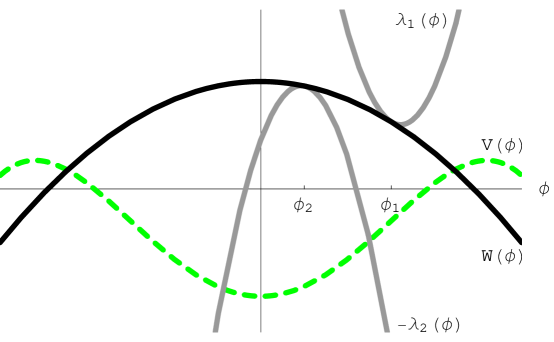
Figure 2: Sample $W$ (solid line), $V$ (dotted line), $\lambda_{1}$ and $\lambda_{2}$ (grey lines) as functions of $\phi$. By adjusting the integration constant of (8) one can arrange for $\lambda_{1}$ to be tangent to $W$, but then for $\lambda_{2}$ also to be tangent amounts to a fine-tuning.

It should be kept in mind that we are working strictly at the classical level. If we tune parameters so that $W(\phi)$ and $-\lambda_{2}(\phi)$ are tangent, then loop corrections to $\lambda_{\alpha}(\phi)$ and $V(\phi)$ must be expected to spoil the relation.

It is true that if this fine-tuning can be achieved, there is no cosmological constant allowed in the four-dimensional action. A quick way to see this is to show that the lagrangian is a total derivative with respect to $r$ when (8), (9), and (10) are satisfied: then the four-dimensional lagrangian must vanish. Let us define

$${\hat{W}(\phi,r)=\left\{\vbox{\openup 3.0pt\halign{\strut$\displaystyle{{}#}$\hfil\quad& \hbox{#}\cr W(\phi)&for $0<r<r_{0}$ \cr-W(\phi)&for $r_{0}<r<2r_{0}$\ , \cr}}\right.}$$

(13)

which is appropriately ${\bf Z}_{2}$ odd. Then it is straightforward to show that

$${{\cal L}}$$

(14)

In (14) we have used (8) (with $W$ replaced by $\hat{W}$) but not (9). If the perfect squares in (14) vanish, then we have

$${1\over 2}{\partial\hat{W}\over\partial r}=W(\phi_{1})\delta(r-r_{1})-W(\phi_{2})\delta(r-r_{2})=\sum_{\alpha}\lambda_{\alpha}\delta(r-r_{\alpha})\,,$$ (15)

where in the second equality we have used the jump conditions, (10). In comparing with (13), recall that by convention $r_{1}=0$ and $r_{2}=r_{0}$.

The form of (14) makes it clear that (9) are indeed a sort of BPS condition for solutions of (6). However, because the perfect squares in (14) come in with opposite signs, there is no obvious analog of a Bogomolnyi bound. Another important implication of (14) is that the total action of any configuration of flat branes vanishes. This is even true of non-periodic arrays provided $A\to-\infty$ as $r\to\pm\infty$.

3.2 Non-zero cosmological constant

The fine-tuning to achieve zero cosmological constant was already commented on in [3]. The purpose of this section is show that if the fine-tuning is imperfect, then there are solutions without rolling moduli but where the metric on the branes is de Sitter space or anti-de Sitter space.

Most of the analysis is similar to section 3.1, so we will be brief. The metric ansatz is

$$ds^{2}=e^{2A(r)}\bar{g}_{ij}dx^{i}dx^{j}-dr^{2}\ ,$$ (16)

where $\bar{g}_{ij}$ is the metric of four-dimensional de Sitter or anti-de Sitter spacetime: $\bar{R}_{ij}=-3\bar{\Lambda}\bar{g}_{ij}$, where $\bar{\Lambda}$ is the four-dimensional cosmological constant (positive for de Sitter spacetime and negative for anti-de Sitter spacetime). Explicitly, we may write the four-dimensional metrics as

$${dS_{4}:}$$

(17)

The five-dimensional Ricci tensor and the equations of motion are

$${R_{ij}=e^{2A}\left(4A^{\prime 2}+A^{\prime\prime}-3\bar{\Lambda}e^{-2A}\right)\bar{g}_{ij}\,,\qquad R_{55}=-4A^{\prime 2}-4A^{\prime\prime}\,,} {\phi^{\prime\prime}+4A^{\prime}\phi^{\prime}} {{}={\partial V(\phi)\over\partial\phi}+\sum_{\alpha}{\partial\lambda_{\alpha}(\phi)\over\partial\phi}\delta(r-r_{\alpha})\,,} {A^{\prime\prime}+\bar{\Lambda}e^{-2A}} {{}=-{2\over 3}\phi^{\prime 2}-{2\over 3}\sum_{\alpha}\lambda_{\alpha}(\phi)\delta(r-r_{\alpha})\,,} {A^{\prime 2}-\bar{\Lambda}e^{-2A}} {{}=-{1\over 3}V(\phi)+{1\over 6}\phi^{\prime 2}\ .}$$ (18)

The jump conditions (7) are unchanged. Neither $A(r)$ nor $|\bar{\Lambda}|$ can be determined unambiguously from the equations of motion because they enter only in the combination $A(r)-{1\over 2}\ln|\bar{\Lambda}|$. We will see that this combination is what determines the four-dimensional cosmological constant in four-dimensional Planck units. We could adjust the additive constant on $A$, if we so desired, to set $\bar{\Lambda}=1$ for de Sitter spacetime or $\bar{\Lambda}=-1$ for anti-de Sitter spactimee. The important point is not to count the magnitude of $\bar{\Lambda}$ as an adjustable parameter separate from the additive constant on $A$.

Already from (18) we can see why there should be a solution with no fine-tuning of parameters. The $\phi$ equation and the zero-energy condition together have three integration constants, and there is also the brane separation $r_{0}$. Because $A$ itself rather than just its derivatives enters into the equations (18), the additive constant on $A$ is no longer trivial. As before there are four boundary conditions (two jump conditions at each brane), so generically one expects a (locally) unique solution for any given $V(\phi)$, $\lambda_{1}(\phi)$ and $\lambda_{2}(\phi)$.

The solution in the bulk (more precisely, in region $A$ of figure 1) can still be obtained as a solution of a slightly modified system of first order equations,

$$A^{\prime} = -\frac{1}{3}\,W\,\gamma(r)\,,$$ (19)

$$\phi^{\prime} = {1\over 2\gamma(r)}\,{\partial W\over\partial\phi}\,,$$

$$V = \frac{1}{8\gamma(r)^{2}}\left(\frac{\partial W}{\partial\phi}\right)^{2}-\frac{1}{3}\,W^{2}\,,$$

which differ from (9) just by inclusion of the factor

$$\gamma(r)\equiv\sqrt{1+\frac{9\bar{\Lambda}}{W(r)^{2}}\,e^{-2A(r)}}\,.$$ (20)

Note that this completely changes the character of the problem. In the case of zero cosmological constant, the first order equations (8), (9) allowed us to find solutions for given $V$ directly by first integrating (8) to solve for $W(\phi)$, then using the equations (9) to solve consecutively for $\phi(r)$ and $A(r)$. We now see that if we do not fine-tune the cosmological constant to zero, we obtain a complicated non-linear first order system of differential equations for 3 functions $W(r)$, $\phi(r)$ and $A(r)$, now viewed as functions of a single independent variable $r$, which we cannot simply solve for in sequence. $V(\phi)$ is still to be considered the information that is put in from the Lagrangian, but its relationship with $W$ can no longer be isolated from the rest of the system. Derivatives with respect to $\phi$ should now be thought of as

$$\frac{\partial}{\partial\phi}=\frac{1}{\phi^{\prime}(r)}\frac{\partial}{\partial r}.$$ (21)

To make this point more transparent, it is useful to rewrite the system (19) as an autonomous system, that is in the form

$$A^{\prime}=f(A,W,\phi),\,\qquad\phi^{\prime}=g(A,W,\phi),\,\qquad W^{\prime}=h(A,W,\phi)\,,$$ (22)

where

$$f(A,W,\phi) = -\frac{1}{3}\,\gamma(r)\,W(r)\,,$$ (23)

$$g(A,W,\phi) = \sqrt{2\,V(\phi(r))+\frac{2}{3}\,W(r)^{2}}\,,$$

$$h(A,W,\phi) = 2\gamma(r)\left(2\,V(\phi(r)+\frac{2}{3}\,W(r)^{2}\right)\,.$$

While for a generic $V(\phi)$ this system will still be hard to solve, it is very well suited for generating examples where $V(\phi)$ is determined at the end. For any given shape of the warp factor $A(r)$ one desires, one can find a potential that supports such a solution by the following procedure: pick $A(r)$, calculate $A^{\prime}(r)$, solve $A^{\prime}=-\frac{W}{3}\gamma$ algebraically for $W(r)$, and use $\phi^{\prime}=\sqrt{\frac{W^{\prime}}{2\gamma}}$ to obtain $\phi(r)$. $V(r)$ can now simply be determined by plugging in $W$ and $\phi$, and after inverting $\phi(r)$ to $r(\phi)$ one obtains the desired $V(\phi)$. This procedure for example can be used to generate fat branes (as we will discuss them in later chapters for the Minkowski case) with an AdS or dS worldvolume. Note that this simple technique for generating examples is not possible in the obvious first order system one could write down simply by introducing one new variable $y$ with the one new defining equation $y=\phi^{\prime}$, as it is a standard technique for converting a system of higher order equations into a first order system.

Assuming (19), the jump conditions reduce to

$${\lambda_{1}(\phi(0))} {{}=W(r=0)\gamma(0),} {{\partial\lambda_{1}\over\partial\phi}(\phi(0))} {{}=\frac{1}{\gamma(0)}\frac{\partial W}{\partial\phi}\Bigg{|}_{\phi(0)}\,,} {\lambda_{2}(\phi(r_{0}))} {{}=W(r=r_{0})\gamma(r_{0}),} {{\partial\lambda_{2}\over\partial\phi}(\phi(r_{0}))} {{}=\frac{1}{\gamma(r_{0})}\frac{\partial W}{\partial\phi}\Bigg{|}_{\phi(r_{0})}\ .}$$ (24)

If for a given $V(\phi)$ we fix $A(0)$ arbitrarily, then the 5 other initial conditions, $\phi(0)$, $A^{\prime}(0)$, $W(0)$, $W^{\prime}(0)$, $\phi(0)$, $\phi^{\prime}(0)$ can be determined up to discrete choices, using the 3 equations from (19) evaluated at $r=0$ and the 2 from the first line of (24). Then (22) can be solved unambiguously for $\phi(r)$, $W(r)$ and $A(r)$. $r_{0}$ is fixed by the last equality in (19). One is left with one condition, namely the third equality in (24). It is a (very complicated) constraint on $A(0)$, which generically will have only discretely many solutions. The point is that we wind up with exactly as many parameters as constraints, so it doesn’t take any fine-tuning to get a solution.

There does not seem to be a simple way to express the action as a sum (or difference) of squares plus total derivatives, in analogy to (14). However it is straightforward to use the equations of motion to show that

$${{\cal L}}$$

(25)

When ${\cal L}$ is integrated over the $S^{1}$ parametrized by $r$, it must for consistency reduce to the four-dimensional lagrangian,

$$\bar{\cal L}={1\over 4\pi G_{4}}\sqrt{|\det\bar{g}_{ij}|}\left[-{1\over 4}\bar{R}-{3\over 2}\bar{\Lambda}\right]\ ,$$ (26)

evaluated on de Sitter or anti-de Sitter spacetime, where $\bar{R}_{ij}=-3\bar{\Lambda}\bar{g}_{ij}$, with $\bar{\Lambda}$ positive or negative, respectively. Comparison yields the relation

$${1\over G_{4}}=4\pi\int dr\,e^{2A}\ ,$$ (27)

where as usual the $r$ integration is over the whole of $S^{1}$. For consistency with observation we must demand the bound

$${1\over G_{4}|\bar{\Lambda}|}\mathrel{\mathstrut\smash{\ooalign{\raise 2.5pt\hbox{$>$}\cr\lower 2.5pt\hbox{$\sim$}}}}\left({\ell_{\rm Hubble}\over\ell_{\rm 4d\ Planck}}\right)^{2}\approx 10^{120}\ .$$ (28)

In view of (27) this translates to

$$4\pi\int dr\,e^{2\left(A(r)-{1\over 2}\ln|\bar{\Lambda}|\right)}\mathrel{\mathstrut\smash{\ooalign{\raise 2.5pt\hbox{$>$}\cr\lower 2.5pt\hbox{$\sim$}}}}10^{120}\ .$$ (29)

The function $A(r)-{1\over 2}\ln|\bar{\Lambda}|$ is fixed by (19) and (24) once $V(\phi)$, $\lambda_{1}(\phi)$, and $\lambda_{2}(\phi)$ are specified. A dramatic fine-tuning in these quantities is required to achieve (29).

In general it is difficult to obtain solutions to (18) or (19) in closed form. We can however give a complete treatment of the case where there is no scalar and $W$ is just a constant (namely the square root of the bulk cosmological constant); see also [16, 17]. In this case the only equations we have to solve are the first equations in each line of (19) and (24). The solutions can be expressed as follows:

$${{}dS_{4}:\quad\bar{\Lambda}>0}$$

(30)

In the $dS_{4}$ case it is necessary to restrict $r_{0}<r_{1}$. The main point which (30) demonstrates is the following. Suppose one starts with any fixed negative bulk cosmological constant, $-4/L^{2}$, and arbitrary but specified $\lambda_{1}$ and $\lambda_{2}$, subject only to the constraint that if one of the $\lambda_{\alpha}$ exceeds $3/L$ in magnitude, then the other must also exceed $3/L$ in magnitude and be of the opposite sign. Then there is a unique solution to (30) up to the usual ambiguity between the additive constant on $A$ and the magnitude of $\bar{\Lambda}$. Both $r_{1}$ and $r_{0}$ will be fixed in this solution, and so will the combination $A-{1\over 2}\ln|\bar{\Lambda}|$ which determines the four-dimensional cosmological constant in Planck units. The only exception is when $\lambda_{1}=-\lambda_{2}={3\over L}$: in this case the branes are flat, $r_{1}$ is a meaningless additive constant on $A$, and the brane separation $r_{0}$ is not fixed.

The bulk solutions in (30) have vanishing Weyl tensor, hence they are locally $AdS_{5}$. All we have found, then, is an embedding of $AdS_{4}$ and $dS_{4}$ as codimension one hypersurfaces in $AdS_{5}$. To verify this one can find an explicit change of variables which brings the bulk metric into the standard form

$$ds^{2}=e^{-2\tilde{r}/L}(d\tilde{t}^{2}-d\tilde{x}_{1}^{2}-d\tilde{x}_{2}^{2}-d\tilde{x}_{3}^{2})-d\tilde{r}^{2}\ .$$ (31)

If we demand that the map from untilded to tilded coordinates be orientation preserving, then the natural choice is

$${{}dS_{4}:} {{}\tilde{t}=-\sqrt{\bar{\Lambda}}\mathop{\rm coth}\nolimits{r_{1}-r\over L}e^{-\sqrt{\bar{\Lambda}}t}\ ,\quad\tilde{r}=-\sqrt{\bar{\Lambda}}Lt-L\log\sinh{r_{1}-r\over L}\ ,} {{}\tilde{x}_{1}=x_{1}\ ,\quad\tilde{x}_{2}=x_{2}\ ,\quad\tilde{x}_{3}=x_{3}} {{}AdS_{4}:} {{}\tilde{x}_{3}=\sqrt{-\bar{\Lambda}}\tanh{r_{1}-r\over L}e^{\sqrt{-\bar{\Lambda}}x_{3}}\ ,\quad\tilde{r}={\sqrt{-\bar{\Lambda}}}Lx_{3}-L\log\cosh{r_{1}-r\over L}\ ,} {{}\tilde{t}=t\ ,\quad\tilde{x}_{1}=x_{1}\ ,\quad\tilde{x}_{2}=x_{2}\ .}$$ (32)

Let us now focus on the $dS_{4}$ case with one positive and one negative tension brane at the ends of the bulk. A solution of the form (30) maps to a strip of the $\tilde{t}-\tilde{r}$ plane between two curves of the form $\tilde{t}=-c_{\alpha}e^{\tilde{r}/L}$. Here $c_{1}$ and $c_{2}$ are positive constants. Because $\partial/\partial\tilde{t}$ is a Killing vector of the bulk geometry, we can trivially obtain a broader class of solutions which have as their boundaries curves of the form $\tilde{t}-\tilde{t}_{\alpha}=-c_{\alpha}e^{\tilde{r}/L}$, where now $\tilde{t}_{1}$ and $\tilde{t}_{2}$ are additional constants, only one of which can be set to $0$ through diffeomorphism freedom. In these solutions the proper distance between the branes is not constant. In fact, generically the branes intersect at some point, or they intersect the boundary of $AdS_{5}$ at different points—or both. In the latter case the graviton bound state ceases to exist at some finite time as measured on the negative tension brane. This reinforces the intuition that brane-world cosmology can encounter some curious pathologies.

The strategy of displacing one boundary by some distance along the flow of a Killing vector of $AdS_{5}$ can also be applied to flat branes. For instance, one could shift the negative tension brane forward along the global time of $AdS_{5}$ to obtain a new solution where the proper distance between the branes is non-constant. The positive and negative tension branes would then intersect at some time in the distant past, and the positive tension brane would again retreat to the true boundary of $AdS_{5}$ at a finite time as measured on the negative tension brane. This is a catastrophe since it means that gravity would cease altogether in four dimensions: the four-dimensional Planck length would vanish.

4 An explicit model

It is useful now to turn to an explicit example with non-trivial dynamics for a single scalar. For simplicity, we choose quadratic $W(\phi)$, $\lambda_{1}(\phi)$, and $\lambda_{2}(\phi)$ which are tangent to one another in the manner illustrated in figure 2. Explicitly,

$${W(\phi)}$$

(33)

We stress that the physical properties of the model are summarized by $V(\phi)$ and the $\lambda_{\alpha}(\phi)$: in the absence of supersymmetry, there is no preferred choice of $W(\phi)$. In section 4.2 we will analyze the different possible $W(\phi)$ that lead to the particular quartic $V(\phi)$ exhibited in (33). Until then we will just assume that the particular $W(\phi)$ that is tangent to $\lambda_{1}(\phi)$ happens to be the quadratic one shown in (33). We make this assumption in order to obtain solutions in closed form. The only physical fine-tuning is the requirement that $-\lambda_{2}(\phi)$ is also tangent to $W(\phi)$. The quantities $L$, $b$, $\phi_{1}$, $\phi_{2}$, $\gamma_{1}$, and $\gamma_{2}$ are parameters of the various potentials, and no dimensionless ratio of them should be large if we want to preserve naturalness.

We will always assume that $\gamma_{1}$ and $\gamma_{2}$ are positive so that the energetics of $\lambda_{1}$ and $\lambda_{2}$ tend to stabilize the positions of the branes in field space. We will usually assume $b>0$ as well. It should be noted that $V(\phi)$ is unbounded below, as is common and without pathology in $AdS$ supergravity.

4.1 Analytical calculations

It is trivial to solve the first order equations (9) in the model (33) to obtain

$${\phi(r)}$$

(34)

The brane spacing is determined by the condition $br_{0}=\ln(\phi_{1}/\phi_{2})$. The difference $A(0)-A(r_{0})$ gives the number of $e$-foldings in discussions [1, 9] of the gauge hierarchy problem, and one easily obtains

$$A(0)-A(r_{0})={1\over bL}\ln{\phi_{1}\over\phi_{2}}-{1\over 6}(\phi_{1}^{2}-\phi_{2}^{2})\ .$$ (35)

Phenomenologically one wants

$$A(0)-A(r_{0})\approx\ln{M_{\rm Planck}\over M_{\rm electroweak}}\approx 37\ .$$ (36)

If $b>0$, then $\phi_{1}^{2}-\phi_{2}^{2}>0$, and only first term can contribute to the hierarchy. This is conceivable if $bL$ is fairly small: for instance, if $\phi_{1}/\phi_{2}=e$ then one needs $bL\approx 1/37$. If $b<0$, then both terms in (35) could contribute to the hierarchy. One could for instance obtain an acceptable hierarchy by taking $bL=1$, $\phi_{1}=1$, and $\phi_{2}=15$.

The treatment of [3] ignored back-reaction of the scalar profile on the geometry. Crudely speaking this means one should drop the second term in (35) since it came from a term proportional to the square of the scalar field in (34). More precisely, (14) of [3] can be reproduced exactly by dropping the second term in (35) and identifying their $m^{2}L^{2}$ with our $bL$ in the limit of small $bL$. Thus the analysis of [3] was essentially adequate for the case $b>0$, where to obtain a large hierarchy one wants a bulk geometry which is not so far from $AdS_{5}$ that the second term of (35) is large. However the inclusion of back-reaction becomes quite important in the $b<0$ case, where a large hierarchy can be most easily obtained via a geometry which deviates strongly from $AdS_{5}$.

Any mechanism for generating large numbers must be probed for robustness. We may ask, once the hierarchy (36) is obtained, how much can the parameters change and still give the same weak scale to within errors? For definiteness, let us ask what change of parameters shifts $A(0)-A(r_{0})$ by no more than $0.02$: this would amount to a shift of the weak scale by two percent, which is about the ratio of the $Z$ width to its mass. In the $b>0$ scenario we described above, a change of $\phi_{1}/\phi_{2}$ by about one part in $2000$ changes the weak scale by two percent: multiplicative shifts in this ratio are magnified by the factor $1/bL$. In the $b<0$ scenario, changing $\phi_{2}$ by about one percent changes the weak scale by two percent. Thus (superficially at least) the $b<0$ scenario is more robust.

4.2 Numerics

We now change gears and refocus on (8). The purpose is to illustrate the problem of selecting a superpotential $W(\phi)$ which reproduces a given potential function $V(\phi)$. However, we shall be content to explore this question only in the model of this section, where $V(\phi)$ is given in (33). It is convenient to rescale variables, partly to prepare for use of the MATLAB linked program DFIELD5 [19]. We therefore define

$${\phi}$$

(37)

We denote the rescaled preferred superpotential by $x_{0}(t)$ since we will consider other superpotentials corresponding to the potential $U(t)$.

In this notation (8) takes the form

$$\left({dx\over dt}\right)^{2}=x(t)^{2}+U(t)\,.$$ (38)

There is a sign ambiguity in taking the square root which must be kept in mind, but we will discuss only the features of the differential equation which results from the positive root, namely

$${dx\over dt}=\sqrt{x^{2}-{1\over b^{2}L^{2}}+\left(1+{4\over bL}\right){t^{2}\over 16}-{t^{4}\over 64}}\,.$$ (39)

The equation is roughly like the energy equation in the mechanics problem of a particle in an inverted harmonic potential. As in mechanics there are forbidden regions of the $t-x$ plane where $x^{2}+U(t)<0$. At a boundary of this region, which would be a turning point in a mechanics problem, the slope ${\textstyle{dx\over dt}}$ vanishes. According to the general theory of first order differential equations there is a unique solution curve through every point not in a forbidden region. The inequality

$$\left|{dx\over dt}\right|\leq|x|+\sqrt{|U(t)|}\,,$$ (40)

shows that no solution reaches $|x|=\infty$ at a finite field value.

The DFIELD5 program quite rapidly provides a reasonable global and quantitative picture of the space of solutions. The quantities of our problem depend only on the single dimensionless parameter $bL$, and we set $bL=1$ in our numerical work.

Figure 3: The $t$–$x$ plane, showing forbidden regions.

A large-scale plot of the $t$–$x$ plane is shown in figure 3, and we see two large forbidden regions on the left and right and a small one in the center. The inclined lines at a grid of points are the slopes, obtained from (39), of the solution curves through each point. The solution through $(t,x)=(0,1)$ is shown, and it is easy to see that it gives the preferred superpotential $x_{0}(t)=1-t^{2}/8$ only for $t<0$. This is related to the sign ambiguity of the square root in (39), and it is not a difficulty for us because we are primarily concerned with the region $t<0$ which includes the full range of the geometry containing two branes which was discussed in the first part of this section.

Some other representative solutions are also plotted in figure 3. It is not proven, but it appears to be the case that the only solutions which give a superpotential defined on the full field space $-\infty<t<\infty$ are the curve through $(t,x)=(0,1)$ and its mirror image through $(t,x)=(0,-1)$, which is also shown in figure 3. Other solution curves reach the boundary of the allowed region at a finite value of $t$ in one direction, and one can see that $x^{\prime}(t)$ vanishes but $x^{\prime\prime}(t)$ diverges as one approaches the boundary. By examining an approximate form of (39) and (9) $\!,$ one can show that these curves approach the boundary at a finite value of the coordinate $r$. It then appears that the solution curve reflects, and one must consider solutions of (39) with the other sign of the square root. The scale factor $A(r)$ is smooth at the turning point. This issue does not affect our application, since the full brane geometry is contained in a region without turning points.

Let’s recall the logic of our construction. The potential $V(\phi)$ and left-hand brane tension $\lambda_{1}(\phi)$ are matched at a chosen value $\phi=\phi_{1}$. We then choose the unique superpotential $W(\phi)$ which satisfies $W(\phi_{1})=\lambda_{1}(\phi_{1})$ and agrees in sign of slope with $\lambda_{1}^{\prime}(\phi_{1})$. Agreement in the magnitude of the slope is guaranteed by (8) and (12). We then integrate the first order equations (9) which gives the unique solution of the second order problem (6) with the initial conditions $\phi(0)=\phi_{1}$, $\phi^{\prime}(0)=\lambda_{1}^{\prime}(\phi_{1})$, the latter from the jump condition (7). For consistency, it is useful to know that any other choice of $W(\phi)$ leads to a different solution of (6), one which does not satisfy the jump conditions. This is quite clear from figure 3, since the jump conditons. e.g. (10), are no longer satisfied if we change solution chosen at the relevant fixed value $t_{1}=\sqrt{8/3}\,\phi_{1}$.

We have explored our suggested solution generating technique in only one model. Global issues associated with the turning points do not spoil the applicability of our method, and the method is certainly easy to use in the reverse mode where we start with a conveniently chosen $W(\phi)$. We believe that this favorable situation is generic.

5 Smooth solutions modeling branes

So far we have been considering solutions to an action that contains explicit $\delta$-functions at the positions of the branes. One might wonder to what extent this approach has already built in the answers one wants to obtain. The purpose of this section is to present a one-parameter family of purely 5d Lagrangians for gravity coupled to a scalar, labelled by the parameter $\beta$, whose solutions are generically smooth and asymptote to a specific $\delta$-brane solution of the type considered so far. For generic $\beta$, the smoothed branes appear as domain walls interpolating between various scalar vacuua. In the “stiff” limit ($\beta\rightarrow\infty$) the second derivative of the scalar potential goes to infinity, so the scalar becomes very heavy and can be integrated out. The parameters entering the scalar potential become the brane tensions and positions associated with $\delta$-function terms in an action of the type (1) + (3) after integrating out the scalar.

Several comments are in order. First, as mentioned before, we will not be able to treat negative tension branes in this framework. Second, the solutions presented in this section do not have any fields living on the brane, since the smooth solitons that in the stiff limit become the branes do not have any zero modes. Both these obstacles can be avoided by introducing “by hand” the $\delta$-functions in the action, but this is precisely what we want to avoid with the smooth formalism. In principle, the second limitation above could be overcome by studying a more complicated smooth model which allows for non-trivial zero modes on the brane.

Last but not least we should emphasize that even though we are considering once more 5d gravity coupled to a scalar, this time the scalar should not be thought of as the bulk scalar $\phi$ we studied so far, which plays the role of a modulus for the fifth dimension. Instead it is the scalar that the branes are made of! In order to avoid confusion we will call this auxiliary scalar $\xi$ and reserve the symbol $\phi$ for the modulus scalar. In the stiff limit, where the soliton approaches the array of localized $\delta$-like branes the fluctuations of $\xi$ are frozen out. The bulk scalar $\phi$ has to be introduced as a second scalar. Interactions localized on the brane, like the $\lambda(\phi)$ we introduced earlier, can be mimicked by coupling the bulk scalar $\phi$ only to derivatives of $\xi$.

We study a five-dimensional action of the form

$$S=\int_{M}d^{4}x\;dr\sqrt{|\mbox{det}g_{\mu\nu}}\left[-\frac{1}{4}R+\frac{1}{2}(\partial\xi)^{2}-V(\xi)\right].$$ (41)

We will work in the first order framework and hence take $V(\xi)$ to be given in terms of a “superpotential” as in (8) and study solutions to the first order equations (9). We will show that once we specify the potential appropriately, the resulting solitonic solution describing an array of branes with tension $\lambda_{\alpha}$ at positions $r_{\alpha}$ in the fifth dimension is specified uniquely.

We are interested in the case where the scalar profile is given as a solitonic domain wall configuration interpolating between various vacua for the scalar field, e.g. written as

$$\xi(r)=\sum_{\alpha}\frac{1}{\sqrt{\beta}}\;\kappa_{\alpha}\;\mbox{tanh}(\beta(r-r_{\alpha})),$$ (42)

or a similar function that has the properties that

• in the “stiff” limit ($\beta\rightarrow\infty$) it reduces to an array of step functions of height $\sim\frac{\kappa_{\alpha}}{\sqrt{\beta}}$, and that

• its first derivative is always negative and approaches a collection of $\delta$-functions at position $r_{\alpha}$ of strength $\sim\frac{\kappa_{\alpha}}{\sqrt{\beta}}$.

Note that latter property requires all $\kappa_{\alpha}$ to be positive, ensuring that the function $\xi(r)$ is invertible. This solution in the stiff limit becomes an array of branes of tension

$$\lambda_{\alpha}=\frac{4}{3}\kappa_{\alpha}^{2}$$ (43)

and only positive tensions appear.

Can we find a $W(\xi)$ in such a way that it allows a solution of the form specified in (42)? In order to do so, we just rewrite the first order equation for the scalar flow in (9) as

$$2\xi^{\prime} = \frac{\partial W(\xi)}{\partial\xi}=\frac{\partial W(\xi(r))}{\partial r}\frac{\partial r(\xi)}{\partial\xi}=\frac{W^{\prime}}{\xi^{\prime}}$$ (44)

$$W(r) = 2\int^{r}(\xi(r^{\prime})^{\prime})^{2}\;dr^{\prime}.$$ (45)

Using invertibility of $\xi(r)$ we can re-express $W(r)$ as $W(\xi)$ and hence obtain a potential $V(\xi)$ which leads to a solution of the desired form. The one integration constant in $W$ corresponds to an “overall” bulk cosmological constant. It should be chosen in such a way that $A^{\prime}(r)=-\frac{1}{3}W(r)$ is positive (negative) to the left (right) of all branes. Since $A^{\prime\prime}$ is always negative, it is always possible to choose the integration constant this way. As we will see in the next section this property is enough to ensure that there exists a 4-dimensional graviton. Now we can turn the philosophy around and say that once we have specified $V$ and hence specified the action, or more precisely the bulk cosmological constant and the cosmological constants between the various branes given in terms of the value of $V(\xi)$ at its minima, the first order equations then provide us with a solution of the form (42) for $\xi(r)$ together with the $A(r)$. In the stiff limit this solution approaches an array of sharply localized branes at positions $r_{\alpha}$ and tensions $\lambda_{\alpha}$.

One should think of $V(\xi)$ as being obtained from integrating out the microscopic physics. One then can ask again whether there is some dynamical principle that determines the parameters in $V$. Since we expressed $W$ as an integral over $(\xi^{\prime})^{2}$ those parameters are the $\kappa_{\alpha}$ and the $r_{\alpha}$. Calculating the action integral of the solution as a function of $\kappa_{\alpha}$ and $r_{\alpha}$ one finds once more that it is always zero. We remain with a serious fine-tuning problem: the underlying theory has to be arranged in such a way, that for given $\lambda_{\alpha}$ and $r_{\alpha}$ the potential has precisely the form specified by (45). In the stiff limit all that remains of $V$ are its values at the minima – the inter-brane cosmological constants – and the fine-tuning problem reduces to the standard fine-tuning of the bulk cosmological constants against the brane tensions.

For example, in the case of a single brane we start with

$$\xi(r)=\frac{\kappa}{\sqrt{\beta}}\ \mbox{tanh}(\beta r)\,,$$ (46)

leading to

$$\xi^{\prime}(r)=\kappa\ \frac{\sqrt{\beta}}{\mbox{cosh}^{2}(\beta r)}\,,$$ (47)

and hence

$$W=2\kappa^{2}\int(\xi^{\prime})^{2}\;dr=2\kappa^{2}\left(\mbox{tanh}(\beta r)-\frac{1}{3}\mbox{tanh}^{3}(\beta r)\right)=2\kappa\sqrt{\beta}(\xi-\frac{\beta}{3\kappa^{2}}\,\xi^{3})\,.$$ (48)

$A$ is simply obtained by integrating $W$. In the multi-brane arrays the solution becomes slightly more complicated due to the cross-terms in $(\xi^{\prime})^{2}$ but it is still analytical. One can show that in the stiff limit all possible smoothings lead to the same brane array.

Before we end our discussion on smoothing of the singular solutions, let us comment on how the coupling to the additional bulk scalar looks in this framework. In order to mimic the localized interactions for the bulk scalar $\phi$ we couple it to the derivatives of the auxiliary scalar $\xi$. Basically, this means that we couple a $\sigma$-model for the scalars to gravity, where the kinetic terms of the auxiliary scalar $\xi$ depend on the bulk scalar $\phi$. In the stiff limit this once more will reduce to the solutions discussed in the previous sections.

Similar to (8) and (9) we can find a first order formalism for the general action

$$S=\int_{M}d^{4}xdr\sqrt{|\mbox{det}g_{\mu\nu}|}\left[-\frac{1}{4}R+\frac{1}{2}G_{IJ}\partial^{\mu}\phi^{J}\partial_{\mu}\phi^{I}-V(\phi)\right]\,,$$ (49)

where $G_{IJ}$ is a metric on the scalar target space. Any solution to

$$(\phi^{I})^{\prime}={1\over 2}\,G^{IJ}\,{\partial W(\phi)\over\partial\phi^{J}}\,,\qquad A^{\prime}=-{1\over 3}W(\phi)\,,$$ (50)

is also a solution to the full second order equations provided $V$ is of the special form

$$V(\phi)={1\over 8}\,G^{IJ}\,{\partial W(\phi)\over\partial\phi^{I}}\,{\partial W(\phi)\over\partial\phi^{J}}-{1\over 3}W(\phi)^{2}\ .$$ (51)

Choosing a two scalar model with $\phi^{1}=\phi$ and $\phi^{2}=\xi$ and choosing $G_{12}=G_{21}=0$, $G_{11}=1$ and $G_{22}(\phi)$ to be an arbitrary function of $\phi$ we should once more be able (50) to engineer a smooth model, this time limiting to multi-brane-array in the presence of the bulk scalar $\phi$ with localized interactions.

A count of parameters similar to the ones in section 3.1 and 3.2 allows us to conclude that—at least locally—any solution of the equations of motion following from (49) which preserves $3+1$-dimensional Poincaré invariance can be written as a solution of (50) for an appropriately chosen $W(\phi)$ satisfying (51). Suppose there are $n$ scalars involved in the action (49). Each of them satisfies a second order equation of motion. The scale factor $A$ satisfies a first-order zero-energy constraint analogous to the last line of (6). So there are $2n+1$ integration constants. One of them can be absorbed into an additive shift on $r$. Now, (50) leads to only $n+1$ integration constants since the scalar equations are now first order. But there are also $n$ integration constants in (51) regarded as a partial differential equation for $W(\phi)$. Again one integration constant can be absorbed into an additive shift on $r$. The point is that either way we have the same number of integration constants, so barring non-generic phenomena and global obstructions, the solution spaces are the same.

This is quite an interesting result in view of the AdS/CFT correspondence [20, 21, 22]. One of the main puzzles in the correspondence is how one might translate the renormalization group (RG) equations, which are first order, into supergravity equations, which are second order. In [14] first order equations were extracted from the conditions for unbroken supersymmetry. These equations are suggestive of an RG flow based on the gradient of a c-function. The c-function is $W(\phi)$, and its relation to the conformal anomaly arises because of the equation $A^{\prime}=-{1\over 3}W$: in regions where the scalars are nearly constant and the geometry is nearly $AdS_{5}$, an application of the analysis of [23] shows that the Weyl anomaly coefficients in the conformal field theory are proportional to the third power of the radius of $AdS_{5}$, or equivalently to $|W|^{-3}$. (Thus in a sense it would be more appropriate to speak of $|W|^{-3}$ as the c-function.)

In a non-supersymmetric “flow,” the c-function can still be defined [24, 14] as $-3A^{\prime}$, and it is possible to demonstrate $A^{\prime\prime}\leq 0$ using only the weakest of positive energy conditions [14]. But then the spirit of RG is lost: one wants to have a notion of a first order flow through the space of possible theories labelled by different values of parameters, and whatever c-function one constructs should be defined in terms of those parameters. The construction of $W$ indicated in (51) seems to realize this idea explicitly.

However there are some caveats. First, $W$ depends on $n$ integration constants, where as before $n$ is the number of scalars. It seems reasonable that these integration constants can be interpreted as specifying the state of the dual field theory, which does not change under RG—only the Hamiltonian evolves. Second, the same phenomena of forbidden regions and turning points that we discussed in section 4.2 occur also in the case of several scalars. A forbidden region is a region of $(W,\phi)$ space where $V(\phi)+{1\over 3}W^{2}$ is negative. Barring singular behavior in $G_{IJ}$, one finds that the gradient of $W$ vanishes at the border of these regions, so no flow can cross over. Rather, flows reflect from the border and the subsequent flow is controlled by a different branch of $W$. Because of the multi-valued nature of $W$, we do not regard (50) as a wholly satisfactory starting point for the transcription of supergravity equations into RG equations. However it is perhaps a step in the right direction.

6 Fluctuations around the solution

Finally we examine the equations governing fluctuations of the metric and scalar around the classical background solutions of the equations of motion of the action (4). Our methods are somewhat different from those in the literature. We choose an axial-type gauge, and the resulting form of the four-dimensional graviton is particularly simple. Transverse traceless modes in general obey the equation of a massless scalar in the curved background, and by recasting this as the Schrödinger equation for a supersymmetric quantum mechanics problem, we argue that there are no space-like modes threatening stability.

We impose the “axial gauge” constraint, so named for its resemblance to $A_{3}=0$ in electrodynamics:

$$h_{\mu 5}=0\,,$$ (52)

where $\mu=0,1,2,3,5$. We can then write the total metric in the form

$$ds^{2}=e^{2A(r)}(\eta_{ij}+h_{ij})\,dx^{i}dx^{j}-dr^{2}\,,$$ (53)

where we extracted a factor $e^{2A}$ from the fluctuation term to simplify future equations. Axial gauge is not a total gauge fix, as diffeomorphisms generated by a vector field $\epsilon_{i}=e^{2A(r)}\,\omega_{i}(x^{j})$, $\epsilon_{5}=0$ preserve the condition (52) while transforming the fluctuations $h_{ij}$ as

$$h_{ij}(x^{k},r)\rightarrow h_{ij}(x^{k},r)+\partial_{i}\,\omega_{j}(x^{k})+\partial_{j}\,\omega_{i}(x^{k})\,.$$ (54)

Note the resemblance to four-dimensional diffeomorphisms.

The Ricci tensor can be computed from the metric (53). To zeroth order in the fluctuations we continue to have (5), while to first order we calculate (using Maple):

$${R_{ij}^{\>(1)}}$$

(55)

where $\mathop{\mathchoice{\vbox{\vbox{\hrule height=0.6pt\hbox{\vrule width=0.6pt,height=5.0pt\kern 5.0pt\vrule width=0.6pt} \hrule height=0.6pt}}}{\vbox{\vbox{\hrule height=0.6pt\hbox{\vrule width=0.6pt,height=5.0pt\kern 5.0pt\vrule width=0.6pt} \hrule height=0.6pt}}}{\vbox{\vbox{\hrule height=0.4pt\hbox{\vrule width=0.4pt,height=3.75pt\kern 3.75pt\vrule width=0.4pt} \hrule height=0.4pt}}}{\vbox{\vbox{\hrule height=0.4pt\hbox{\vrule width=0.4pt,height=3.0pt\kern 3.0pt\vrule width=0.4pt} \hrule height=0.4pt}}}\,}\nolimits=\eta^{ij}\partial_{i}\partial_{j}$ is the flat four-dimensional Laplacian. Einstein’s equations in Ricci form require that $R_{\mu\nu}=\bar{T}_{\mu\nu}\equiv T_{\mu\nu}-{1\over 3}\,g_{\mu\nu}\,T^{\,\alpha}_{\;\;\,\alpha}$, and we find

$${\bar{T}_{ij}^{\>(1)}}$$

(56)

Additionally, the equation of motion for the scalar fluctuation $\tilde{\phi}$ is

$$e^{-2A}\,\mathop{\mathchoice{\vbox{\vbox{\hrule height=0.6pt\hbox{\vrule width=0.6pt,height=5.0pt\kern 5.0pt\vrule width=0.6pt} \hrule height=0.6pt}}}{\vbox{\vbox{\hrule height=0.6pt\hbox{\vrule width=0.6pt,height=5.0pt\kern 5.0pt\vrule width=0.6pt} \hrule height=0.6pt}}}{\vbox{\vbox{\hrule height=0.4pt\hbox{\vrule width=0.4pt,height=3.75pt\kern 3.75pt\vrule width=0.4pt} \hrule height=0.4pt}}}{\vbox{\vbox{\hrule height=0.4pt\hbox{\vrule width=0.4pt,height=3.0pt\kern 3.0pt\vrule width=0.4pt} \hrule height=0.4pt}}}\,}\nolimits\,\tilde{\phi}-\tilde{\phi}^{\prime\prime}-4A^{\prime}\tilde{\phi}^{\prime}+\left({\partial^{2}V(\phi)\over\partial\phi^{2}}+\sum_{\alpha}{\partial^{2}\lambda(\phi)\over\partial^{2}\phi}\delta(r-r_{\alpha})\right)\tilde{\phi}={1\over 2}\phi^{\prime}\eta^{ij}h_{ij}^{\prime}\,.$$ (57)

The equation $R_{ij}^{\>(1)}=\bar{T}_{ij}^{\>(1)}$ further simplifies as a consequence of the zeroth-order equation of motion (6) :

$$A^{\prime\prime}+4A^{\prime 2}=-{4\over 3}V(\phi)-{2\over 3}\sum_{\alpha}\lambda_{\alpha}(\phi)\delta(r-r_{\alpha})\,,$$ (58)

to

$${e^{2A}\left(\frac{1}{2}\partial_{r}^{2}+2A^{\prime}\partial_{r}\right)h_{ij}-{1\over 2}\mathop{\mathchoice{\vbox{\vbox{\hrule height=0.6pt\hbox{\vrule width=0.6pt,height=5.0pt\kern 5.0pt\vrule width=0.6pt} \hrule height=0.6pt}}}{\vbox{\vbox{\hrule height=0.6pt\hbox{\vrule width=0.6pt,height=5.0pt\kern 5.0pt\vrule width=0.6pt} \hrule height=0.6pt}}}{\vbox{\vbox{\hrule height=0.4pt\hbox{\vrule width=0.4pt,height=3.75pt\kern 3.75pt\vrule width=0.4pt} \hrule height=0.4pt}}}{\vbox{\vbox{\hrule height=0.4pt\hbox{\vrule width=0.4pt,height=3.0pt\kern 3.0pt\vrule width=0.4pt} \hrule height=0.4pt}}}\,}\nolimits}$$

(59)

Let us now consider the transverse traceless components of $h_{ij}$, defined by the non-local projection [26]:

$${\overline{h}_{ij}=\left({1\over 2}(\pi_{ik}\,\pi_{jl}+\pi_{il}\,\pi_{jk})-{1\over 3}\pi_{ij}\,\pi_{kl}\right)\,h^{kl}=h_{ij}+\ldots\,,}$$

(60)

where $\pi_{ij}\equiv(\eta_{ij}-\partial_{i}\partial_{j}/\mathop{\mathchoice{\vbox{\vbox{\hrule height=0.6pt\hbox{\vrule width=0.6pt,height=5.0pt\kern 5.0pt\vrule width=0.6pt} \hrule height=0.6pt}}}{\vbox{\vbox{\hrule height=0.6pt\hbox{\vrule width=0.6pt,height=5.0pt\kern 5.0pt\vrule width=0.6pt} \hrule height=0.6pt}}}{\vbox{\vbox{\hrule height=0.4pt\hbox{\vrule width=0.4pt,height=3.75pt\kern 3.75pt\vrule width=0.4pt} \hrule height=0.4pt}}}{\vbox{\vbox{\hrule height=0.4pt\hbox{\vrule width=0.4pt,height=3.0pt\kern 3.0pt\vrule width=0.4pt} \hrule height=0.4pt}}}\,}\nolimits)$ and $\ldots$ indicates nonlocal terms. The $\overline{h}_{ij}$ satisfy

$$\partial^{j}\overline{h}_{ij}=\eta^{ij}\,\overline{h}_{ij}=0\,.$$ (61)

We emphasize that $(\ref{TT})$ applies only to the components defined in (60)  and is not a gauge choice; it would be incompatible with (52) and the residual gauge freedom (54).

For the $\overline{h}_{ij}$, (59) simplifies enormously. The transverse traceless projection removes the right-hand side, and we are left with

$$\left(\partial_{r}^{2}+4A^{\prime}\partial_{r}-e^{-2A}\mathop{\mathchoice{\vbox{\vbox{\hrule height=0.6pt\hbox{\vrule width=0.6pt,height=5.0pt\kern 5.0pt\vrule width=0.6pt} \hrule height=0.6pt}}}{\vbox{\vbox{\hrule height=0.6pt\hbox{\vrule width=0.6pt,height=5.0pt\kern 5.0pt\vrule width=0.6pt} \hrule height=0.6pt}}}{\vbox{\vbox{\hrule height=0.4pt\hbox{\vrule width=0.4pt,height=3.75pt\kern 3.75pt\vrule width=0.4pt} \hrule height=0.4pt}}}{\vbox{\vbox{\hrule height=0.4pt\hbox{\vrule width=0.4pt,height=3.0pt\kern 3.0pt\vrule width=0.4pt} \hrule height=0.4pt}}}\,}\nolimits\right)\overline{h}_{ij}=0\,.$$ (62)

Notice that all $\delta$-function jumps have canceled out; this is nothing but the equation of motion for a free massless scalar in our curved background. In an $AdS_{5}$ black hole background, the spin-2 components of the graviton were also found to obey a free scalar wave equation [27, 28].

We expect one solution of our equations to be the four-dimensional graviton. Since it is massless in the four-dimensional sense, it must obey $\mathop{\mathchoice{\vbox{\vbox{\hrule height=0.6pt\hbox{\vrule width=0.6pt,height=5.0pt\kern 5.0pt\vrule width=0.6pt} \hrule height=0.6pt}}}{\vbox{\vbox{\hrule height=0.6pt\hbox{\vrule width=0.6pt,height=5.0pt\kern 5.0pt\vrule width=0.6pt} \hrule height=0.6pt}}}{\vbox{\vbox{\hrule height=0.4pt\hbox{\vrule width=0.4pt,height=3.75pt\kern 3.75pt\vrule width=0.4pt} \hrule height=0.4pt}}}{\vbox{\vbox{\hrule height=0.4pt\hbox{\vrule width=0.4pt,height=3.0pt\kern 3.0pt\vrule width=0.4pt} \hrule height=0.4pt}}}\,}\nolimits\overline{h}_{ij}=0$. We can easily see that such a solution to (62) is simply the $r$-independent plane wave

$$\overline{h}_{ij}=C_{ij}\,e^{ipx}\,,$$ (63)

where $p^{2}=0$ and $C_{ij}$ is a constant. Thus in this presentation the phenomenological graviton has a very simple form.

As we will argue below, the norm of metric fluctuations is

$$||\,\overline{h}\,||^{2}=\int dr\,e^{2A(r)}\,\overline{h}_{ij}\,\overline{h}^{ij}\,,$$ (64)

where indices are raised with $\eta^{ij}$. We see that the graviton mode (63) is normalizable because the $r$-direction is effectively compactified in these models. The $S^{1}/Z^{2}$ geometries are manifestly compact. For arrays of positive-tension branes only, the range of $r$ is $-~{}\infty~{}<~{}r~{}<~{}\infty$, but the norm converges if we restrict to cases where

$${A^{\prime}\rightarrow 1/L_{-}>0\quad}$$

(65)

which are asymptotically anti-de Sitter geometries. In all such models, which include the smooth configurations of section 5, there is a naturally massless four-dimensional graviton as described above.

Having identified the four-dimensional graviton, we next turn to the question of stability. If the equations of motion were to admit fluctuations with a space-like momentum, it would be evident that the zeroth-order solution — our classical background — is not stable. For the transverse traceless components, we can cast the expression (62) in the form of a supersymmetric quantum mechanics problem, where $p^{2}$ plays the role of the energy, and thus argue that $p^{2}\geq 0$.

To accomplish this, we first need to eliminate the factor $e^{2A}$ multiplying the momentum. We can do this by changing variables to coordinates in which the background is conformally flat:

$$ds^{2}=e^{2A(z)}\left((\eta_{ij}+h_{ij})\,dx^{i}dx^{j}-dz^{2}\right)\,.$$ (66)

Now (62) takes the form

$$(-\partial_{z}^{2}-3\,A^{\prime}(z)\,\partial_{z}+\mathop{\mathchoice{\vbox{\vbox{\hrule height=0.6pt\hbox{\vrule width=0.6pt,height=5.0pt\kern 5.0pt\vrule width=0.6pt} \hrule height=0.6pt}}}{\vbox{\vbox{\hrule height=0.6pt\hbox{\vrule width=0.6pt,height=5.0pt\kern 5.0pt\vrule width=0.6pt} \hrule height=0.6pt}}}{\vbox{\vbox{\hrule height=0.4pt\hbox{\vrule width=0.4pt,height=3.75pt\kern 3.75pt\vrule width=0.4pt} \hrule height=0.4pt}}}{\vbox{\vbox{\hrule height=0.4pt\hbox{\vrule width=0.4pt,height=3.0pt\kern 3.0pt\vrule width=0.4pt} \hrule height=0.4pt}}}\,}\nolimits)\,\overline{h}_{ij}=0\,.$$ (67)

In terms of $H_{ij}(z)=e^{-ipx}\,e^{3A/2}\,h_{ij}$, this becomes

$$\left(-\partial_{z}^{2}+{9\over 4}A^{\prime}(z)^{2}+{3\over 2}A^{\prime\prime}(z)\right)H_{ij}(z)=p^{2}H_{ij}(z)\,.$$ (68)

This differential operator has the same form as a Hamiltonian in quantum mechanics, with a potential $V(z)={\textstyle{9\over 4}}A^{\prime}(z)^{2}+{\textstyle{3\over 2}}A^{\prime\prime}(z)$ and $p^{2}$ as the energy eigenvalue. One can easily check that it factorizes

$$\left((\partial_{z}+{3\over 2}A^{\prime}(z))(-\partial_{z}+{3\over 2}A^{\prime}(z))\right)H_{ij}(z)=p^{2}H_{ij}(z)\,.$$ (69)

In flat space, these terms are one another’s adjoint, and (69) can be regarded as a factorization of the Hamiltonian into $\overline{Q}Q$. This is supersymmetric quantum mechanics, and the transformed graviton wave-function is the supersymmetric ground state. However, to complete the argument we must show that a flat-space norm is correct for $H_{ij}(z)$ in our curved background.

In Lorentzian signature field theory, the norm of fluctuations is determined by the requirement that formally conserved quantities such as the contraction $T^{\mu\nu}K_{\nu}$ of the stress tensor and a Killing vector of the background have convergent integral

$$\int dz\,d^{3}x\,\sqrt{g}\,T^{0\nu}\,K_{\nu}\,,$$ (70)

over a constant time 4-surface and vanishing flux through its boundary 3-surface. Stress tensors for metric fluctuations are complicated, but in this linearized situation the stress tensor must be covariantly conserved for all solutions of the equation of motion (62) or (67) - (68) . Thus for the Killing vector ($K^{0}=0$, $K^{i}=$constant, $K^{5}=0$) of spatial translations parallel to the domain wall, one can take the form

$$T^{0}_{i}=e^{-2A}\,\partial_{0}\overline{h}_{kl}\,\partial_{i}\overline{h}^{kl}\,,$$ (71)

obtained by specializing the obvious covariant expression for $T^{0}_{i}$ to our description of the background. (The index $i$ takes values 1,2,3 in (71)  while $k$, $l$ are raised with $\eta^{kl}$.) The requirement of a convergent integral for the spatial momentum carried by the fluctuation then constrains the radial eigenfunctions $H_{ij}(z)$ to satisfy

$$\int dz\,H_{ij}\,H^{ij}\,=\mbox{ finite}.$$ (72)

which is the usual Schrödinger norm for (68) (and equivalent to (64) when rephrased in terms of $\overline{h}_{ij}$ and the radial coordinate $r$). Supersymmetric quantum mechanics thus ensures that there are no normalizable modes with $p^{2}<0$. Thus we can state that there are no transverse traceless modes with space-like momentum that might destabilize the backgound solution.

Before concluding this section, we briefly remark on the non-transverse traceless components of the metric fluctuation, which are coupled to the scalar by the equations (55), (56), and (57). These coupled equations are not easy to solve, and we have not attempted to rule out tachyonic modes of these fluctuations here.

However, it seems likely that the Boucher non-supersymmetric positive-energy theorem [31, 32] can be extended to include actions such as ours with potentials localized on hypersurfaces, in which case stability would be guaranteed for our solutions, by virtue of their satisfying the first-order equations.

Note Added

As this manuscript was nearing completion, several papers appeared [33, 34, 35, 36] which overlap somewhat with our results. For instance, (14) was also derived in [36], and the $dS_{4}$ solution in (30) was also obtained in [33]. In [35], solutions similar to the single domain wall of section 5 were shown to emerge from a $U(1)$ gauged supergravity theory.

The coupled equations relating scalar and non-transverse metric fluctuations have recently been studied in [37]. The equations can again be reduced to the form of supersymmetric quantum mechanics, and consequently there are no normalizable spacelike modes. Thus our backgrounds have been shown to be entirely free from tachyonic fluctuations.

References

- [1] L. Randall and R. Sundrum, “A Large mass hierarchy from a small extra dimension,” hep-ph/9905221.
- [2] L. Randall and R. Sundrum, “An Alternative to compactification,” hep-th/9906064.
- [3] W. D. Goldberger and M. B. Wise, “Modulus stabilization with bulk fields,” hep-ph/9907447.
- [4] M. Cvetic and H. H. Soleng, “Supergravity domain walls,” Phys. Rept. 282 (1997) 159, hep-th/9604090.
- [5] A. Lukas, B. A. Ovrut, K. S. Stelle, and D. Waldram, “The universe as a domain wall,” Phys. Rev. D59 (1999) 086001, hep-th/9803235.
- [6] A. Kehagias, “Exponential and power-law hierarchies from supergravity,” hep-th/9906204.
- [7] J. Polchinski and E. Witten, “Evidence for heterotic - type I string duality,” Nucl. Phys. B460 (1996) 525–540, hep-th/9510169.
- [8] P. Horava and E. Witten, “Heterotic and type I string dynamics from eleven- dimensions,” Nucl. Phys. B460 (1996) 506–524, hep-th/9510209.
- [9] J. Lykken and L. Randall, “The Shape of gravity,” hep-th/9908076.
- [10] J. Dai, R. G. Leigh, and J. Polchinski, “New connections between string theories,” Mod. Phys. Lett. A4 (1989) 2073–2083.
- [11] P. J. Steinhardt, “General considerations of the cosmological constant and the stabilization of moduli in the brane world picture,” hep-th/9907080.
- [12] C. Csaki and Y. Shirman, “Brane junctions in the Randall-Sundrum scenario,” hep-th/9908186.
- [13] A. Brandhuber and K. Sfetsos, “Nonstandard compactifications with mass gaps and Newton’s law,” hep-th/9908116.
- [14] D. Z. Freedman, S. S. Gubser, K. Pilch, and N. P. Warner, “Renormalization group flows from holography supersymmetry and a c theorem,” hep-th/9904017.
- [15] R.C. Myers, unpublished notes, April 1999.
- [16] T. Nihei, “Inflation in the five-dimensional universe with an orbifold extra dimension,” hep-ph/9905487.
- [17] N. Kaloper, “Bent domain walls as brane-worlds,” hep-th/9905210.
- [18] T. jun Li, “Gauge hierarchy from AdS(5) universe with three-branes,” hep-th/9908174.
- [19] D. Arnold and J. Polking, Ordinary Differential Equations using MATLAB. Prentice Hall, Upper Saddle River, 1999. DFIELD5 is available at http://math.rice.edu/~polking/.
- [20] J. Maldacena, “The Large N limit of superconformal field theories and supergravity,” Adv. Theor. Math. Phys. 2 (1998) 231, hep-th/9711200.
- [21] S. S. Gubser, I. R. Klebanov, and A. M. Polyakov, “Gauge theory correlators from noncritical string theory,” Phys. Lett. B428 (1998) 105, hep-th/9802109.
- [22] E. Witten, “Anti-de Sitter space and holography,” Adv. Theor. Math. Phys. 2 (1998) 253, hep-th/9802150.
- [23] M. Henningson and K. Skenderis, “The Holographic Weyl anomaly,” JHEP 07 (1998) 023, hep-th/9806087.
- [24] L. Girardello, M. Petrini, M. Porrati, and A. Zaffaroni, “Novel local CFT and exact results on perturbations of N=4 superYang Mills from AdS dynamics,” JHEP 12 (1998) 022, hep-th/9810126.
- [25] J. Garriga and T. Tanaka, “Gravity in the brane-world,” hep-th/9911055.
- [26] D. Anselmi, “Central functions and their physical implications,” JHEP 05 (1998) 005, hep-th/9702056.
- [27] N. R. Constable and R. C. Myers, “Spin two glueballs, positive energy theorems and the AdS/CFT correspondence,” hep-th/9908175.
- [28] R. C. Brower, S. D. Mathur, and C.-I. Tan, “Discrete spectrum of the graviton in the AdS(5) black hole background,” hep-th/9908196.
- [29] C. Csaki, J. Erlich, T. J. Hollowood, and Y. Shirman, “Universal aspects of gravity localized on thick branes,” hep-th/0001033.
- [30] A. G. Cohen and D. B. Kaplan, “Solving the hierarchy problem with noncompact extra dimensions,” Phys. Lett. B470 (1999) 52, hep-th/9910132.
- [31] W. Boucher, “Positive energy without supersymmetry,” Nucl. Phys. B242 (1984) 282.
- [32] P. K. Townsend, “Positive energy and the scalar potential in higher dimensional (super)gravity theories,” Phys. Lett. 148B (1984) 55.
- [33] H. B. Kim and H. D. Kim, “Inflation and gauge hierarchy in Randall-Sundrum compactification,” hep-th/9909053.
- [34] H. Hatanaka, M. Sakamoto, M. Tachibana, and K. Takenaga, “Many brane extension of the Randall-Sundrum solution,” hep-th/9909076.
- [35] K. Behrndt and M. Cvetic, “Supersymmetric domain wall world from D = 5 simple gauged supergravity,” hep-th/9909058.
- [36] K. Skenderis and P. K. Townsend, “Gravitational stability and renormalization group flow,” hep-th/9909070.
- [37] O. DeWolfe and D. Z. Freedman, “Notes on fluctuations and correlation functions in holographic renormalization group flows,” hep-th/0002226.