Abstract

We introduce an explicit form of the multi-instanton weight including also instanton–anti-instanton interactions for arbitrary $N_{c}$ in the two-dimensional $CP^{N_{c}-1}$ model. To that end, we use the parametrization of multi-instantons in terms of instanton ‘constituents’ which we call ‘zindons’ for short. We study the statistical mechanics of zindons analytically (by means of the Debye-Hückel approximation) and numerically (running a Metropolis algorithm). Though the zindon parametrization allows for a complete ‘melting’ of instantons we find that, through a combination of dynamical and purely geometric factors, a dominant portion of topological charge is residing in well-separated instantons and anti-instantons.

1 Introduction

In the last two decades there have been much evidence that the specific fluctuations of the gluon field carrying topological charge, called instantons, play a very important role in the dynamics of QCD, the theory of strong interactions [1, 2]. Instantons are most probably responsible for one of the main features of strong interactions, namely for the spontaneous breaking of chiral symmetry [3]. Whether they play a role in the confinement property of QCD is, however, not clear. The difficulty in addressing this problem may be connected to the fact that, strictly speaking, the multi-instanton solution in the vacuum is not known. Instead, in a dilute-gas approximation, one treats the instanton vacuum as a superposition of one-instanton solutions. For large distances the one-instanton gluon field falls off as $A_{\mu}(x)\sim 1/x^{3}$, which means that correlations between instantons at large distances are vanishing in the dilute-gas picture. However, the confinement phenomenon by itself seems to indicate that certain correlations of gluon fields do not fall off when the distance is increased. Therefore, if instantons are of any relevance to confinement, it cannot be seen in the dilute-gas approximation: one has to enrich the arsenal of instanton methods.

This motivates us to study a system where the multi-instanton solution is known, where one can find many features of the strong interaction, and which is simple enough to allow for analytic solutions in some limits. Such a system is provided by the two-dimensional $CP^{N_{c}-1}$ model. This model is known to possess both asymptotic freedom and instantons. Contrary to the $d=4$ Yang–Mills theory where the multi-instanton solutions are not available in an explicit form, in the $CP^{N_{c}-1}$ model they are known explicitly, and for any ‘number of colors’ $N_{c}$ [4, 5]. Moreover, the multi-instanton weight arising from integrating out quantum oscillations about instantons is also known [6, 7, 8]. In addition, the model is exactly solvable at large $N_{c}$ [5, 9], and the spectrum is known for all $N_{c}$ [10]. Therefore, the model is well suited to monitor instantons in a controllable way. It should be added that the model has been much studied by lattice simulations (see, e.g. [11, 12, 13]), and instantons have been identified there by a ‘cooling’ procedure [14].

Since the pioneering paper of Fateev, Frolov and Schwartz [6] it has been known that the multi-instanton system in the $O(3)$ sigma model resembles that of a two-dimensional Coulomb plasma; it can be exactly bosonized to produce a sine-Gordon theory. In a true vacuum, however, one has both instantons and anti-instantons; such a system can be bosonized and solved exactly only at a specific value of the coupling [15] which may not be realistic. Therefore, the general case still remains a difficult and unsolved dynamical problem.

In Sec. 2 we overview the $CP^{N_{c}-1}$ model. In Sec. 3 we derive the general partition function for the $CP^{N_{c}-1}$ in terms of a special form of instanton variables, which are called ‘zindons’. In Sec. 4 we shall describe an approximation to the partition function called the Debye-Hückel approximation, which is capable to account for many features of the instanton ensemble. However, that approximation is in general insufficient. Therefore, in this paper we combine analytical study of the instanton–anti-instanton ensemble with a numerical simulation. In Sec. 5 we describe the Metropolis algorithm used to study the behavior of the model in Monte Carlo simulations. It will turn out that, strictly speaking, the instanton ensemble does not exist for $N_{c}=2$ and that a regularization procedure is required to yield meaningful results. In Sec. 6 we consider the question whether the system has a thermodynamically stable density, i.e., whether the average number of instantons and anti-instantons grows proportional to the volume of the system. Finally in Sec. 7 we have a look at the size distribution, both seen from the instanton input and from the topological charge density.

2 The $CP^{N_{c}-1}$ model

For a number of colors $N_{c}$ the main objects of the $CP^{N_{c}-1}$ model are $N_{c}$ complex fields $v_{A}(x),A=1,\dots,N_{c}$. Defining the norm $|v|^{2}=\sum_{A=1}^{N_{c}}|v_{A}|^{2}$ one can introduce the normalized fields $u_{A}$, a projector P and the unitary operator G via:

$$u_{A}=v_{A}/|v|,\qquad P_{AB}=u_{A}u^{*}_{B},\qquad G=1-2P,$$

$$P^{2}=P=P^{\dagger},\qquad G=G^{\dagger},\qquad G^{2}=1.$$ (1)

One can introduce a vector potential $A_{\mu}$ and a covariant derivative $\nabla_{\mu}$:

$$A_{\mu}=\frac{i}{2}(u_{A}\partial_{\mu}u^{*}_{A}-u^{*}_{A}\partial_{\mu}u_{A}),\qquad\nabla_{\mu}=\partial_{\mu}-iA_{\mu},\qquad(\mu=1,2)\;.$$ (2)

$A_{\mu}$ is a real field, depending on the x-space variables $x$ and $y$ that can be identified with the complex variables $z=x+iy$ and $z^{*}=x-iy$. The field strength tensor and the topological charge density are:

$$F_{\mu\nu}=\partial_{\mu}A_{\nu}-\partial_{\nu}A_{\mu},\;\;\;\;\;\;q(x)=\frac{1}{4\pi}\epsilon_{\mu\nu}F_{\mu\nu}=\frac{-i}{2\pi}\epsilon_{\mu\nu}\partial_{\mu}u_{A}^{*}\partial_{\nu}u_{A}.$$ (3)

The theory is determined by the action

$$S=\int d^{2}x\sum_{A=1}^{N_{c}}|\nabla_{\mu}u_{A}|^{2}=\frac{1}{8}\int d^{2}x{\rm Tr}\left[\partial_{\mu}G\partial_{\nu}G\right],$$ (4)

and the partition function is:

$${\cal Z}=\int\!Du_{A}(x)Du^{*}_{A}(x)DA_{\mu}(x)\delta(|u|^{2}-1)\exp\left(-\frac{1}{g^{2}}\int\!d^{2}x|\nabla_{\mu}u_{A}|^{2}\right)$$

$$=\int\!Du_{A}(x)Du^{*}_{A}(x)\delta(|u|^{2}-1)\exp\left(-\frac{1}{8g^{2}}\int\!d^{2}x{\rm Tr}[\partial_{\mu}G\partial_{\nu}G]\right).$$ (5)

This formulates a nonlinear theory of self-interacting fields, where the nonlinearity is forced by the condition $|u|=1$. There is a topological charge $Q$ in the theory defined as:

$$Q=\int\!d^{2}x\,q(x)=\frac{1}{2\pi}\oint dx_{\mu}A_{\mu}=\frac{1}{4\pi}\int\!d^{2}x\,\epsilon_{\mu\nu}F_{\mu\nu}=\frac{i}{16\pi}\int\!d^{2}x\,\epsilon_{\mu\nu}\,{\rm Tr}\left[G\partial_{\mu}G\partial_{\nu}G\right].$$ (6)

Because of its unitarity $G$ has the property $G\partial G=-\partial GG$, which can be used to show:

$$0\leq\int d^{2}x{\rm Tr}\left[\left(\partial_{\mu}G\pm i\epsilon_{\mu\nu}G\partial_{\nu}G\right)\left(\partial_{\mu}G\pm i\epsilon_{\mu\nu}G\partial_{\nu}G\right)\right]=16(S\mp 2\pi Q)\;.$$ (7)

This tells that the minimal action for a given topological charge of a field configuration, i.e. a solution of the equation of motion, is obtained if the field satisfies the self-duality equation:

$$\partial_{\mu}G\pm i\epsilon_{\mu\nu}G\partial_{\nu}G=0\;\;\Leftrightarrow\;\;\partial_{\mu}v\mp i\epsilon_{\mu\nu}\partial_{\nu}v=0.$$ (8)

Introducing the complex derivative $\partial_{z}=(\partial_{x}-i\partial_{y})/2$, it means that one finds two types of solutions:

$$\partial_{z^{*}}v=0\;\longleftrightarrow\;S=2\pi Q$$ (9)

and

$$\partial_{z}v=0\;\longleftrightarrow\;S=-2\pi Q\;,$$ (10)

which are the Cauchy–Riemann conditions [16]. One calls the first an instanton solution and the second one an anti-instanton solution.

3 ‘Zindons’

A general multi-instanton solution of the self-duality Eq. (9) with topological charge $Q=N_{+}$ is a product of monomials in $z$ [6]:

$$v^{inst}_{A}=c_{A}\prod_{i=1}^{N_{+}}(z-a_{Ai}),\;\;\;\;\;A=1,...,N_{c}.$$ (11)

Similarly, a general multi anti-instanton solution of Eq. (10) with topological charge $Q=-N_{-}$ is a product of monomials in the complex conjugate variable $z^{*}$:

$$v_{A}^{anti}=c^{\prime}_{A}\prod_{j=1}^{N_{-}}(z^{*}-b^{*}_{Aj}),\;\;\;\;\;A=1,...,N_{c}.$$ (12)

For a general configuration with $N_{+}$ instantons and $N_{-}$ anti-instantons we shall consider a product Ansatz [15]:

$$v_{A}=\prod_{i=1}^{N_{+}}(z-a_{Ai})\prod_{j=1}^{N_{-}}(z^{*}-b^{*}_{Aj}),$$ (13)

where $a_{iA}$ and $b_{jA}$ are fixed 2-dim points written as complex numbers. Those points have been called ‘instanton quarks’ or ‘instanton constituents’ in the past. We suggest a shorter term zindon to denote these entities, in analogy with similar objects introduced in the Yang–Mills theory [17]. ‘Zindon’ is Tajik or Persian word for ‘castle’ or ‘prison’; they are of relevance to describe confinement in the model. There are, thus, $N_{c}$ types or ‘colors’ of the instanton zindons (denoted by $a_{A}$) and $N_{c}$ types of anti-instanton zindons or anti-zindons (denoted by $b_{A}$).

The action and the topological charge for such a multi-instanton–anti-instanton Ansatz are

$$\left.\begin{array}[]{c}S\\ 2\pi Q\end{array}\right\}=2\int d^{2}x\left[\frac{\sum_{A}|v_{A}|^{2}|\sigma_{A}|^{2}-\left|\sum_{A}|v_{A}|^{2}\sigma_{A}\right|^{2}/|v|^{2}}{|v|^{2}}\right.$$

$$\left.\pm\>\frac{\sum_{A}|v_{A}|^{2}|\tau_{A}|^{2}-\left|\sum_{A}|v_{A}|^{2}\tau_{A}\right|^{2}/|v|^{2}}{|v|^{2}}\right],$$

$$\sigma_{A}=\sum_{i=1}^{N_{+}}\frac{1}{z-a_{Ai}},\qquad\tau_{A}=\sum_{j=1}^{N_{-}}\frac{1}{z^{*}-b^{*}_{Aj}},\qquad|v|^{2}=\sum_{A=1}^{N_{c}}|v_{A}|^{2}.$$ (14)

The topological charge can be immediately found from the Cauchy theorem:

$$Q=\frac{1}{2\pi}\oint dx_{\mu}A_{\mu}=N_{+}-N_{-}\,.$$ (15)

The geometric meaning of the zindon coordinates becomes especially clear if one takes a single-instanton solution, $v_{A}(z)=c_{A}(z-a_{A})$. Putting it into the action Eq. (14) one gets the standard form of the instanton profile,

$$S=2\pi Q=2\int\!d^{2}x\frac{\rho^{2}}{[(x-x_{0})^{2}+\rho^{2}]^{2}}=2\pi,$$ (16)

where the instanton center $x_{0}$ is given by the center of masses of zindons,

$$x_{0\mu}=\frac{\sum_{A=1}^{N_{c}}|c_{A}|^{2}a_{A\mu}}{\sum_{A=1}^{N_{c}}|c_{A}|^{2}},$$ (17)

while the spread of the field called the instanton size $\rho$ is given by the spatial dispersion of zindons comprising the instanton,

$$\rho^{2}=\frac{\sum_{A=1}^{N_{c}}|c_{A}|^{2}|a_{A}-x_{0}|^{2}}{\sum_{A=1}^{N_{c}}|c_{A}|^{2}}=\frac{\sum_{A<B}|c_{A}|^{2}|c_{B}|^{2}|a_{A}-a_{B}|^{2}}{\left(\sum_{A}|c_{A}|^{2}\right)^{2}}.$$ (18)

In Eqs.(17, 18) all coordinates $x_{0},\,a_{A}$ are understood as 2-dimensional vectors. In the multi-instanton case the action and topological charge densities will have extrema not necessarily coinciding with the position of the zindon center of masses. Only when a group of zindons of all $N_{c}$ colors happens to be well spatially isolated from all the rest zindons, in the vicinity of this group one can speak about getting a classical instanton profile (16) with the collective coordinates given by Eqs.(17, 18), the role of the coefficients $c_{A}$ played by a product of separations between a given zindon $a_{Ai}$ and all the rest zindons and anti-zindons,

$$|c_{A}|^{2}=\prod_{i^{\prime}\neq i}^{N_{+}}|a_{Ai}-a_{Ai^{\prime}}|^{2}\prod_{j=1}^{N_{-}}|a_{Ai}-b_{Aj}|^{2}.$$ (19)

As a matter of fact, it means that there is no need in introducing explicitly extra degrees of freedom $c_{A}$. It should be added that in the thermodynamic limit, with the system volume $V$ going to infinity, we expect the number of zindons to be proportional to $V$. Meanwhile, the number of the coefficients $c_{A}$ is fixed (equal to $N_{c}$). Therefore, one can neglect this degree of freedom as it plays no role in the thermodynamic limit; we shall therefore put all $c_{A}=1$.

The quantum determinants in the multi-instanton background, defining the instanton weight or the measure of integration over collective coordinates $a_{Ai}$, has been computed in Ref. [6] in case of $N_{c}=2$ (which is the $O(3)$ sigma model) and in Refs. [7, 8] for arbitrary $CP^{N_{c}-1}$; the results of these references coincide up to notations.

3.1 Multi-instanton weight in the case $N_{c}=2$

In the $N_{c}=2$ case the multi-instanton weight is that of the Coulomb gas [6, 8]:

$${\cal D}a\cdot w_{a}=\prod_{A=1}^{N_{c}=2}\prod_{i=1}^{N_{+}}d^{2}a_{Ai}\cdot\frac{\prod_{A=1,2}\prod_{i<i^{\prime}}|a_{Ai}-a_{Ai^{\prime}}|^{2}}{\prod_{i,i^{\prime}}|a_{1i}-a_{2i^{\prime}}|^{2}}\left[\left(\frac{2\pi}{g^{2}}\Lambda\right)^{2}C(2)\right]^{N_{+}}$$ (20)

where $\Lambda$ is the renormalization-invariant combination of the bare charge $g^{2}$ and of the UV cutoff $M$ needed to regularize the theory; it is the analog of $\Lambda_{QCD}$. The numerical coefficient $C(2)$ depends on the regularization scheme used; in the Pauli–Villars scheme it has been found in Ref. [18] to be

$$C(2)=\left(\frac{2}{e}\right)^{6}\frac{3}{\pi^{2}}=0.04822082\,.$$ (21)

We shall absorb this constant in the definition of $\Lambda$. In the one-loop approximation the charge $g^{2}$ in Eq. (20) remains unrenormalized; in two loops it starts to run. It is interesting that for accidental reasons (the number of zero modes per unit topological charge, equal four, coinciding with the ratio of the second-to-first Gell-Mann–Low coefficients, equal to $b^{\prime}/b=4N_{c}/N_{c}=4$) the coupling $g^{2}$ does not ‘run’ in the two-loop approximation either: $2\pi/g^{2}$ in Eq. (20) should be just replaced by $(b/2)^{b^{\prime}/2b}=1$. For anti-instanton zindons $b_{Aj}$ one has a similar expression, with $N_{+}$ replaced by $N_{-}$. We denote the corresponding weight by ${\cal D}b\cdot w_{b}$.

3.2 Partition function for arbitrary $N_{c}$

The general expression for the multi-instanton weight $w_{a}$ in the $CP^{N_{c}-1}$ model is [7, 8]:

$$w_{a} = \exp\Bigg{[}\sum_{i<j}^{N_{+}}\sum_{A}^{N_{c}}\ln|a_{Ai}-a_{Aj}|^{2}-\frac{N_{c}}{8\pi}\int d^{2}x\ln|v_{A}|^{2}\partial^{2}\ln|v_{A}|^{2}$$

$$-\frac{N_{c}}{2}N_{+}\ln\left(\sum_{A=1}^{N_{c}}|c_{A}|^{2}\right)+\frac{N_{c}}{2}N_{+}+N_{+}\sum_{A=1}^{N_{c}}\ln|c_{A}|^{2}\Bigg{]}\;,$$

$$v_{A} = \prod_{i=1}^{N_{+}}c_{A}(z-a_{Ai})\;.$$ (22)

In the following we set $|c_{A}|=1$ for reasons explained above. The second (integral) term in Eq. (22) can be analytically computed only for $N_{c}=2$; it gives the Coulomb interaction of Eq. (20). For $N_{c}>2$ we approximate the integral term by a simpler explicit expression. To that end, let us consider a configuration with zindons of $N_{c}$ colors forming clusters well separated from each other, see Fig. 1. We denote the centers of clusters by $x_{i}$,

$$x_{i}=\frac{1}{N_{c}}\sum_{A=1}^{N_{c}}a_{Ai}\;,$$ (23)

the sizes of the instantons associated with those clusters by $\rho_{i}$,

$$\rho_{i}^{2}=\frac{1}{N_{c}}\sum_{A=1}^{N_{c}}(a_{Ai}-x_{i})^{2}=\frac{1}{N_{c}^{2}}\sum_{A<B}(a_{Ai}-a_{Bi})^{2}\;,$$ (24)

and the separation between clusters by

$$R_{ij}=|x_{i}-x_{j}|\;,$$ (25)

assuming $R_{ij}^{2}\gg\rho_{i,j}^{2}$. In such geometry the integral term can be easily evaluated, yielding

$$I\{a_{Ai}\} = -\frac{N_{c}}{8\pi}\int d^{2}x\ln|v_{A}|^{2}\partial^{2}\ln|v_{A}|^{2}$$ (26)

$$\simeq -\frac{N_{c}}{2}\Bigg{[}2\sum_{i<j}^{N_{+}}\ln R_{ij}^{2}+\sum_{i=1}^{N_{+}}\ln\rho_{i}^{2}+N_{+}(\ln N_{c}+1)\Bigg{]}+{\cal O}\left(\frac{\rho^{2}_{i,\;j}}{{R_{ij}}^{2}}\right)\;.$$

We would like to write the functional of zindon positions $I\{a_{Ai}\}$ in such a way that it

• depends only on the separations between individual zindons, $a_{Ai}-a_{Bj}\;$;

• is symmetric under permutations of same-color zindons, $(a_{Ai}\leftrightarrow a_{Aj})$;

• reduces to Eq. (26) in the dilute regime;

• at $N_{c}=2$ comes to the exact expression valid for any geometry:

$$I^{N_{c}=2}\{a_{Ai}\}=-\left[\sum_{i,j=1}^{N_{+}}\ln(a_{1i}-a_{2j})^{2}+N_{+}(1-\ln 2)\right]\;.$$ (27)

The solution to this problem is, naturally, not unique. We shall suggest two forms of approximate expressions for $I\{a_{Ai}\}$, both satisfying the above requirements a-d. The first form is

$$I\{a_{Ai}\} = -\frac{N_{c}}{2}\sum_{i,j=1}^{N_{+}}\ln\left[\sum_{A<B}(a_{Ai}-a_{Bj})^{2}\right]+\frac{N_{c}}{2}N_{+}(\ln N_{c}-1)$$ (28)

$$+N_{c}\frac{N_{+}(N_{+}-1)}{2}\ln\frac{N_{c}(N_{c}-1)}{2}\;.$$

Combining it with other terms in (22) we get the following multi-instanton weight:

$$w_{a} = \exp\beta\Bigg{[}\sum_{i<i^{\prime}}^{N_{+}}\sum_{A=1}^{N_{c}}\ln(a_{Ai}-a_{Ai^{\prime}})^{2}\Lambda^{2}-\frac{N_{c}}{2}\sum_{i,i^{\prime}=1}^{N_{+}}\ln\left[\sum_{A<B}^{N_{c}}(a_{Ai}-a_{Bi^{\prime}})^{2}\Lambda^{2}\right]$$ (29)

$$+N_{c}\frac{N_{+}(N_{+}-1)}{2}\ln\frac{N_{c}(N_{c}-1)}{2}\Bigg{]}\;.$$

This form of the interactions between zindons belonging to instantons will be used in computer simulations of the ensemble, see below. This form is, however, inconvenient for analytical estimates since it involves many-body interactions represented by $\ln\sum_{A<B}(a_{Ai}-a_{Bi^{\prime}})^{2}$. Therefore, we suggest a more simple second form involving only two-body interactions:

$$\tilde{I}\{a_{Ai}\}=-\frac{1}{N_{c}-1}\sum_{i,j=1}^{N_{+}}\sum_{A<B}^{N_{c}}\ln(a_{Ai}-a_{Bj})^{2}+\frac{N_{c}}{2}N_{+}(\ln N_{c}-1)\;.$$ (30)

The second form reproduces correctly only the leading term in (22) in the ‘dilute’ regime; however it is exact for $N_{c}=2$. Consequently, the multi-instanton weight can be written in a compact form:

$$\tilde{w}_{a}=\exp\left\{\frac{\beta}{2}\frac{N_{c}}{N_{c}-1}\sum^{N_{+}}_{i,j=1}\sum^{N_{c}}_{A,B=1}{\cal P}_{AB}\ln(a_{Ai}-a_{Bj})^{2}\Lambda^{2}\right\}$$ (31)

Here ${\cal P}_{AB}$ is a projector $N_{c}\times N_{c}$ matrix such that ${\cal P}_{AB}=(N_{c}-1)/N_{c}$ when $A=B$ and ${\cal P}_{AB}=-1/N_{c}$ when $A\neq B$, so that ${\cal P}^{2}={\cal P}$, and ${\cal P}$ has $N_{c}-1$ unit eigenvalues and one zero.

In both forms, (29) and (31), we have introduced an ‘inverse temperature’ $\beta$ for future convenience, in fact $\beta=1$. We have also borrowed certain powers of the scale $\Lambda$ from the overall weight coefficient to make the arguments of the logarithms dimensionless. A comparison of numerical simulations using the weight (29) with analytical calculations using the weight (31) shows that the results do not differ significantly; it means that ensembles generated with the two weights are to a good accuracy equivalent. At $N_{c}=2$ they both coincide with the exact weight (20). For the multi–anti-instanton weight $w_{b}$ one can use either of the forms (29), (31) with an obvious substitution of the instanton-zindon coordinates $a_{Ai}$ by anti-zindon coordinates $b_{Ai}$.

Finally, we turn to the instanton–anti-instanton interaction factor $w_{ab}$. We assume that it is mainly formed by the classical defect of the action,

$$w_{ab}=\exp\left(-\frac{1}{g^{2}}U_{int}(a,b)\right),\;\;\;\;\;U_{int}(a,b)=S_{Ansatz}-2\pi(N_{+}+N_{-}),$$ (32)

where $S_{Ansatz}$ is the action computed on the product Ansatz, (13). Again, it is possible to evaluate this quantity in a regime, when zindons belonging to definite instantons or anti-instantons are grouped together and are well separated from other groups. After some work one obtains the classical interaction potential between zindons and anti-zindons in a form of ‘dipole interactions’ in two dimensions, valid for any number of colors $N_{c}$:

$$U_{int}=8\pi\sum_{all\;I\bar{I}\;pairs}\;\;\frac{1}{N_{c}}\sum_{A}(a_{A}-x_{a})_{\mu}(b_{A}-x_{b})_{\nu}\frac{1}{R^{2}}\left(\delta_{\mu\nu}-2\frac{R_{\mu}R_{\nu}}{R^{2}}\right),$$

$$x_{a}=\frac{a_{1}+...+a_{N_{c}}}{N_{c}},\;\;\;\;\;x_{b}=\frac{b_{1}+...+b_{N_{c}}}{N_{c}},\;\;\;\;\;R_{\mu}=x_{a\mu}-x_{b\mu}.$$ (33)

In terms of zindons, this is a many-body interaction, however, Eq. (33) can be rewritten as a pair interaction of individual zindons, which, naturally, appears to be of a Coulomb type. This is one of the great advantages of using the zindon parametrization of instantons. We rewrite the dipole interaction (33) as a sum of two-body interactions using the $N_{c}\times N_{c}$ projector ${\cal P}_{AB}$ introduced above:

$$U_{int}=-\frac{4\pi}{N_{c}}\sum_{i=1}^{N_{+}}\sum_{j=1}^{N_{-}}\sum_{A,B=1}^{N_{c}}{\cal P}_{AB}\ln|a_{Ai}-b_{Bj}|^{2}.$$ (34)

In the case when groups of $N_{c}$ zindons form clusters well separated from groups of $N_{c}$ anti-zindons, this reduces to the dipole interaction (33). Notice that the interaction of “same-color” zindons is repulsive while that of “different-color” is attractive. At $N_{c}=2$ the projector matrix ${\cal P}_{AB}$ is

$${\cal P}_{AB}^{N_{c}=2}=\frac{1}{2}\left(\begin{array}[]{cc}1&-1\\ -1&1\end{array}\right),$$ (35)

so that the interaction becomes just a sum of Coulomb interactions between charges of different signs. In this case this form has been known previously [18, 15]. In Ref. [15] it has been shown that this form of the interaction possesses an additional conformal symmetry, and one can think that its domain of validity in the zindon configuration space is wider than the one where it has been actually derived. We shall, thus, use for the mixed instanton–anti-instanton weight:

$$w_{ab}=\exp\left\{2\beta\beta_{1}\sum_{i=1}^{N_{+}}\sum_{j=1}^{N_{-}}\sum_{A,B=1}^{N_{c}}{\cal P}_{AB}\ln\left[(a_{Ai}-b_{Bj})^{2}\Lambda^{2}\right]\right\},\quad\beta_{1}=\frac{2\pi}{g^{2}N_{c}}\;.$$ (36)

The full partition function takes the form (for arbitrary instanton angle $\theta$):

$$Z=\sum_{N_{+},N_{-}}\frac{e^{i\theta N_{+}}}{(N_{+}!)^{N_{c}}}\frac{e^{i\theta N_{-}}}{(N_{-}!)^{N_{c}}}\int{\cal D}a{\cal D}b\Lambda^{2N_{c}(N_{+}+N_{-})}w_{a}w_{b}w_{ab}$$ (37)

with $w_{ab}$ given by (36), and $w_{a}$,$w_{b}$ given either by (29) or (31). If one uses the form (31) the interpretation is especially clear: the partition function describes two systems of zindons (instanton and anti-instanton ones) experiencing logarithmic Coulomb interactions, whose strength is $N_{c}-1$ times stronger for same-color zindons than for different-color zindons. One has attraction for zindons–anti-zindons of different color and repulsion for zindons–anti-zindons of the same color. At $N_{c}=2$ one can think of the ensemble as of that of $e^{+},e^{-},\mu^{+},\mu^{-}$ particles [15]. The interaction of opposite-kind zindons are suppressed by an additional factor $\beta_{1}=2\pi/(g^{2}N_{c})$. It is actually a running coupling, depending on the scale in the problem. Since there is only one scale here, the density of zindons at the thermodynamic equilibrium, this $\beta_{1}$ should be found self-consistently from the arising equilibrium density at the end of the calculations.

4 The Debye-Hückel approximation

To get an insight in the dynamics of the system by simple analytical methods we consider here the so-called Debye-Hückel approximation to the partition function (37). Let us consider first a general case of a statistical ensemble of $F$ kinds of particles with two-body interactions given by:

$$U_{\rm int}=\sum_{i\leq j}u_{\rm int}(x_{i}-x_{j})\;.$$ (38)

The number of particles of kind $f$ is $N_{f},f=1,\dots,F$. One writes the partition function for fixed numbers of particles as:

$$Z=e^{-\beta{\cal F}}=\frac{1}{N_{1}!\dots N_{F}!}\int\prod_{f=1}^{F}\prod_{i_{f}=1}^{N_{f}}dx^{f}_{i_{f}}e^{-\beta U_{\rm int}}\;,$$ (39)

where ${\cal F}$ is the Helmholtz free energy and $x^{f}$ are coordinates of particles of kind $f$. The one-particle density of particles of kind $f$ is defined as:

$$n_{f}(x_{1}^{f}) = \frac{1}{Z}\frac{1}{N_{1}!\cdots N_{F}!}\int dx_{2}^{f}\cdots dx_{N_{f}}^{f}\prod_{g\neq f}\prod_{i_{g}=1}^{N_{g}}dx_{i_{g}}^{g}e^{-\beta U_{\rm int}}\;,$$

$$\int dx_{1}^{f}n_{f}(x_{1}^{f}) = 1\;,$$ (40)

which differs from the full partition function by that one does not integrate over the coordinates of one particle of kind $f$. Similarly, one can introduce the two-particle density by avoiding integrating over coordinates of particle $f$ and of particle $g$:

$$n_{fg}(x_{1}^{f},x_{2}^{g})=\frac{1}{Z}\frac{1}{N_{1}!\cdots N_{F}!}\int dx_{2}^{f}\dots dx_{N_{f}}^{f}\>dx_{1}^{g}dx_{3}^{g}\cdots dx_{N_{g}}^{g}\prod_{h\neq f\atop h\neq g}\prod_{i_{h}=1}^{N_{h}}dx_{i_{h}}^{h}e^{-\beta U_{\rm int}}\;.$$ (41)

This function can be written as

$$n_{fg}(x_{1}^{f},x_{2}^{g})=n_{f}(x_{1}^{f})n_{g}(x_{2}^{g})e^{-\beta\omega_{fg}(x_{1}^{f}-x_{2}^{g})}\;,$$ (42)

which serves as a definition of the two-particle correlation function $\omega_{fg}(x_{1},x_{2})$. If this function is zero the particles are not correlated. Introducing, in the similar fashion, higher-order densities, one can derive an (infinite) chain of equation for those densities. The so-called correlation energy is:

$$E_{\rm corr}=-\frac{1}{2}\sum_{fg}\frac{N_{f}N_{g}}{V^{2}}\int\int dx_{1}dx_{2}u_{fg}(x_{1}-x_{2})e^{-\beta\omega_{fg}(x_{1}-x_{2})}\;.$$ (43)

Knowing the correlation energy as function of temperature one can restore the Helmholtz free energy from the general relation:

$$E_{\rm corr}=\frac{\partial}{\partial\beta}(\beta{\cal F})\;.$$ (44)

The Debye-Hückel approximation consists in assuming that $\beta\omega_{fg}$ is small and linearizing the equations [19]. It is usually justified, when the temperature is high, $\beta\rightarrow 0$. In the Debye-Hückel approximation it is also convenient to pass to the Fourier transforms of the pair interaction potential $u_{fg}$ and of the correlation function $\omega_{fg}$. The basic equations from where one finds the correlation functions take the form:

$$\omega_{fg}(k)=u_{fg}(k)+\beta\sum_{h}\frac{N_{h}}{2V}[u_{gh}(-k)\omega_{fh}(k)+u_{fh}(k)\omega_{gh}(-k)]\;.$$ (45)

In our case the particles are zindons belonging either to instantons or to anti-instantons. Let us denote $u_{A_{1}A_{2}},\omega_{A_{1}A_{2}}$ the interaction and the correlation of zindons of color $A_{1}$, $A_{2}$ belonging to instantons. Similarly, $u_{\bar{B}_{1}\bar{B}_{2}},\omega_{\bar{B}_{1}\bar{B}_{2}}$ refer to zindons belonging to anti-instantons. and $u_{A\bar{B}},\omega_{A\bar{B}}$ refer to instanton zindons of color $A$ and anti-instanton zindons of color $\bar{B}$. The approximation is applicable only if all interactions are two-body. For that reason we choose to work with the instanton weights given by Eqs. (31), (36):

$${\cal Z} = \sum_{N_{+},\,N_{-}}\frac{e^{i\theta N_{+}}}{(N_{+}!)^{N_{c}}}\frac{e^{-i\theta N_{-}}}{(N_{-}!)^{N_{c}}}\int{\cal D}a{\cal D}b\;\Lambda^{2N_{c}(N_{+}+N_{-})}\;\tilde{w}_{a}\tilde{w}_{b}w_{ab}\;.$$ (46)

Since our interactions are all of the logarithmic type the Fourier transforms of $u_{fg}$ can be written as:

$$u_{A_{1}A_{2}}(k) = v_{A_{1}A_{2}}\frac{4\pi}{k^{2}},\quad\;v_{A_{1}A_{1}}=1,\quad v_{A_{1}A_{2}}=-\frac{1}{N_{c}-1}\quad{\rm if}\;A_{1}\neq A_{2},$$

$$u_{\bar{B}_{1}\bar{B}_{2}}(k) = v_{\bar{B}_{1}\bar{B}_{2}}\frac{4\pi}{k^{2}},\quad v_{\bar{B}_{1}\bar{B}_{1}}=1,\quad v_{\bar{B}_{1}\bar{B}_{2}}=-\frac{1}{N_{c}-1}\quad{\rm if}\;\bar{B}_{1}\neq\bar{B}_{2},$$

$$u_{A\bar{B}}(k) = v_{A\bar{B}}\frac{4\pi}{k^{2}},\quad v_{A\bar{A}}=2\beta_{1}\frac{N_{c}-1}{N_{c}},\quad v_{A\bar{B}}=-2\beta_{1}\frac{1}{N_{c}}\quad{\rm if}\;A\neq B\;.$$ (47)

It is now convenient to change the notation for the $\omega$ correlation functions to:

$$\omega_{AA}=\omega_{1},\;\;\omega_{AA^{\prime}\atop A\neq A^{\prime}}=\omega_{2},\;\;\omega_{\bar{B}\bar{B}}=\omega_{3},\;\;\omega_{\bar{B}\bar{B}^{\prime}\atop\bar{B}\neq\bar{B}^{\prime}}=\omega_{4},\;\;\omega_{A\bar{B}}=\omega_{5},\;\;\omega_{A\bar{B}^{\prime}\atop\bar{B}^{\prime}\neq A}=\omega_{6}.$$ (48)

The above relations for the $v$’s induce similar relations for the $\omega$’s:

$$\omega_{2}=-\frac{1}{N_{c}-1}\omega_{1},\;\omega_{4}=-\frac{1}{N_{c}-1}\omega_{3},\;\omega_{6}=-\frac{1}{N_{c}-1}\omega_{5}\;.$$ (49)

With the new notations we get the following set of linear equations for the three independent correlation functions $\omega_{1,2,3}$:

$$\beta\omega_{1} = -\gamma[1+\tilde{n}_{+}\beta\omega_{1}+\beta^{\prime}\tilde{n}_{-}\beta\omega_{5}]\;,$$

$$\beta\omega_{3} = -\gamma[1+\tilde{n}_{-}\beta\omega_{3}+\beta^{\prime}\tilde{n}_{+}\beta\omega_{5}]\;,$$

$$\beta\omega_{5} = -\gamma[\beta^{\prime}+\frac{1}{2}\beta^{\prime}\beta(\tilde{n}_{+}\omega_{1}+\tilde{n}_{-}\omega_{3})+\frac{1}{2}\beta\omega_{5}(\tilde{n}_{+}+\tilde{n}_{-})],$$ (50)

where

$$\gamma = \frac{4\pi\beta}{k^{2}},\quad\beta^{\prime}=2\beta_{1}\frac{N_{c}-1}{N_{c}}=\frac{4\pi(N_{c}-1)}{g^{2}N_{c}^{2}}\;.$$

$$\tilde{n}_{+} = \frac{N_{c}}{N_{c}-1}\frac{N_{+}}{V}=\frac{N_{c}}{N_{c}-1}n_{+}\;,\quad\tilde{n}_{-}=\frac{N_{c}}{N_{c}-1}\frac{N_{-}}{V}=\frac{N_{c}}{N_{c}-1}n_{-}\;.$$ (51)

We get the following solutions for the set of linear equations:

$$\omega_{1} = \frac{-4\pi[k^{2}+4\pi\beta\tilde{n}_{-}(1-\beta^{\prime 2})]}{(k^{2}+\kappa_{1}^{2})(k^{2}+\kappa_{2}^{2})}\;,$$

$$\omega_{3} = \frac{-4\pi[k^{2}+4\pi\beta\tilde{n}_{+}(1-\beta^{\prime 2})]}{(k^{2}+\kappa_{1}^{2})(k^{2}+\kappa_{2}^{2})}\;,$$

$$\omega_{5} = \frac{-4\pi\beta^{\prime}k^{2}}{(k^{2}+\kappa_{1}^{2})(k^{2}+\kappa_{2}^{2})}\;,$$

$$\kappa_{1,2} = 2\pi\beta\left[(\tilde{n}_{+}+\tilde{n}_{-})\pm\sqrt{(\tilde{n}_{+}-\tilde{n}_{-})^{2}+4\tilde{n}_{+}\tilde{n}_{-}\beta^{\prime 2}}\;\right]\;.$$ (52)

Returning to the x-space we observe that all correlation functions are exponentially decreasing at large separations between zindons, as contrasted to the original logarithmically growing interactions. This phenomenon is usually referred to as ‘Debye screening’; in our case it takes the particular form of Eq. (52).

Using Eqs. (43,44) one can reconstruct the partition function for a fixed number of instantons and anti-instantons:

$$Z(N_{+},N_{-}) = \exp\left\{-\frac{\beta N_{c}^{2}}{4(N_{c}-1)}V\left[\frac{\tilde{n}_{+}+\tilde{n}_{-}}{2}\left(\ln\frac{\tilde{\Lambda}^{2}}{4\pi\beta\sqrt{\tilde{n}_{+}\tilde{n}_{-}(1-\beta^{\prime 2})}}+1\right)\right.\right.$$

$$\left.\left.-\frac{1}{4}\sqrt{(\tilde{n}_{+}-\tilde{n}_{-})^{2}+4\tilde{n}_{+}\tilde{n}_{-}\beta^{\prime 2}}\;\ln\frac{\kappa_{1}}{\kappa_{2}}\right]\right\}\frac{(V\Lambda^{2})^{N_{c}(N_{+}+N_{-})}}{(N_{+}!)^{N_{c}}(N_{-}!)^{N_{c}}},$$

$$\tilde{\Lambda} = 2\Lambda e^{-\gamma_{E}}\;.$$ (53)

At $N_{+}$=$N_{-}$ = $N/2$ corresponding to the instanton angle $\theta=0$ it simplifies to:

$$Z(N) = \exp\Bigg{[}-\frac{\beta NN_{c}^{3}}{8(N_{c}-1)^{2}}\Bigg{\{}1-\ln\left(\frac{2\pi\beta N_{c}N}{\tilde{\Lambda}^{2}(N_{c}-1)V}\right)$$ (54)

$$-\frac{1}{2}\ln[(1-\beta^{\prime})(1+\beta^{\prime})]-\frac{1}{2}\beta^{\prime}\ln\frac{1-\beta^{\prime}}{1+\beta^{\prime}}\Bigg{\}}\Bigg{]}\frac{(V\Lambda^{2})^{N_{c}N}}{\left(\frac{N}{2}!\right)^{2N_{c}}}\;.$$

Finally, one can find the optimal density of instantons and anti-instantons by maximizing the above partition function in $N$. For a fixed $\beta^{\prime}$ and $\Lambda$ we get then the following density of instantons plus anti-instantons:

$$n=(n_{-}+n_{+})=\frac{<N>}{V\Lambda^{2}}=\Bigg{[}(1+\beta^{\prime})^{\frac{1+\beta^{\prime}}{2}}(1-\beta^{\prime})^{\frac{1-\beta^{\prime}}{2}}4\pi\beta\frac{e^{2\gamma_{E}}}{8}\frac{N_{c}}{N_{c}-1}2^{\frac{8(N_{c}-1)^{2}}{\beta N_{c}^{2}}}\Bigg{]}^{\frac{\beta N_{c}^{2}}{8(N_{c}-1)^{2}-\beta N_{c}^{2}}}\;.$$ (55)

Notice that the density is stable in the thermodynamic limit $V\rightarrow\infty$. At $|\beta^{\prime}|=1$ corresponding to the value of the instanton–anti-instanton interaction constant $\beta_{1}=\pm\frac{N_{c}}{2(N_{c}-1)}$ the system becomes unstable. This could be anticipated from direct inspection of (37): at that value of $\beta_{1}$ the attraction between zindons of different color belonging to instantons and to anti-instantons exceeds the repulsion between same-kind zindons, and the system collapses.

It should be stressed that all quantities involved (like the instanton density $n$, the screening masses $\kappa_{1,2}$ etc.) are stable in the limit $N_{c}\to\infty$. This should be contrasted to the old conjecture by Witten [9] that instantons die out in the large $N_{c}$ limit. Though this conjecture has been criticized later on [20, 21] it remains a widely-believed prejudice.

5 The Metropolis algorithm and regularization procedure

The numerical treatment of instantons in the $CP^{N_{c}-1}$ model is problematic for $N_{c}=2$, where the theory is equal to the two-dimensional $O(3)$ model. The partition function in this case involves a product of integrals of the type $\int d\lambda^{2}/\lambda^{2}$ and is therefore ultraviolet divergent. There are two ways of imposing a regularization. The first consists in decreasing the powers in the interactions (20). Physically, this is equivalent to the introduction of a temperature $T\equiv 1/\beta$, see Eqs. (29),(31), and (36). We reach the physical limit by taking $\beta\rightarrow 1$. For small values of $\beta$ we expect the model to be consistent with the predictions of the Debye-Hückel approximation. The second possibility is using an ultraviolet cutoff $\epsilon$. Technically, this can be easiest done by changing the logarithmic interaction between zindons:

$$\ln(a_{Ai}-a_{Ai^{\prime}})^{2}\rightarrow\ln\left[(a_{Ai}-a_{Ai^{\prime}})^{2}+\epsilon^{2}\right],\quad{\rm etc}\;.$$ (56)

In both cases the physical limit $T\rightarrow 1$ and $\epsilon\rightarrow 0$ does not exist for the free energy, however one can get meaningful results for physical quantities that are connected to derivatives of the free energy. An unpleasant point is that this $\epsilon$ regularization destroys the scaling properties of the theory. We can restore the scaling property by using $\epsilon^{\prime}=\epsilon/L$ as a regularization parameter. Then we restore the original scaling property which we express here in terms of the free energy $F$:

$$F(\epsilon^{\prime},N,L)=\ln Z(\epsilon^{\prime},N,L)=N\ln(L^{2})+\ln z(\epsilon^{\prime},N)\;.$$ (57)

Note that the reduced partition function $z(\epsilon^{\prime},N)$ does no longer depend on $L$. It is exactly this scaling property which will be important later when we try to reconstruct the average density of instantons and anti-instantons in the system. We should emphasize that the price we have to pay for the restoration of the scaling behavior is that the two limits $\epsilon^{\prime}\to 0$ and $L\to\infty$ cannot be interchanged, as with growing L the effective cutoff $\epsilon=\epsilon^{\prime}L$ becomes larger than the average separation between zindons, $\langle R\rangle=1/\sqrt{n}$. However, when $\epsilon^{\prime}$ becomes smaller the physical region where $\epsilon=\epsilon^{\prime}L<\langle R\rangle$ covers larger portions of the configuration space.

To study the behavior of the system numerically we first switch off the interaction between instantons and anti-instantons i.e. we put $\beta_{1}=0$. We then have for $N_{c}=2$ the case of a simple Coulomb gas, where the two different colors interact in the same way as the two different electric charges. In the case of larger $N_{c}$ we have a more complicated ‘multicolor’ interaction which would then require a picture with $N_{c}$ different kind of charges.

The variables of integrations for the theory are the zindon coordinates $a_{Ai}$ and $b_{Ai}$. A direct numerical calculation of the partition function (37) is technically not possible, because the integrand has very sharp maxima: a small variation of the zindon coordinates changes its value by orders of magnitude. Instead of this one can apply a Metropolis algorithm: Starting with a random configuration of zindons, step by step the position of one zindon is varied by a small amount. If the new configuration has a larger value of the weight $w_{a}w_{b}w_{ab}$ then this configuration is accepted, if not then it is only accepted with the probability $w_{a}w_{b}w_{ab}({\rm new})/w_{a}w_{b}w_{ab}({\rm old})$. As Fig. 2 shows, the plateau of important configurations is reached only after 250.000 Metropolis sweeps for $N_{c}=3,4$. In the case $N_{c}=2$ the number of steps necessary to reach the plateau depends on the regularization parameter $\epsilon^{\prime}$: It is large when $\epsilon^{\prime}$ is small. In Fig. 2 we have chosen ${\epsilon^{\prime}}^{2}=0.001$. Already after 20.000 steps one is very close to the plateau here. It is now interesting to make a snapshot of the distribution of the zindons at the plateau region. In Fig. 3 we show snapshots of the zindon ensemble at the plateau region after 500.000 Metropolis steps with $\beta_{1}=0$. Each symbol represents zindons of one color. One observes clearly, that for $N_{c}=2$ zindons of different colors tend to condense into neutral pairs that can be very densely packed. This is the reason for the fact that the partition function is divergent and needs to be regularized in the way described above. Such a condensation does not take place for higher colors $N_{c}=3,4$.

We can put this in a more quantitative way by plotting the free energy $F=\ln Z$ as a function of the regularization parameter $\epsilon$, see Fig. 4. As it should be expected by simple power counting the free energy for the case $N_{c}=2$ diverges proportional to $\ln(\ln(1/\epsilon))$, while it is finite in the case of higher $N_{c}$. In principle such a divergence does not pose a real problem since physical quantities are only related to logarithmic derivatives of the partition function, but it does affect the effectiveness of the numerical studies considerably. In fact, with the computer powers used, it was not possible to go to ${\epsilon^{\prime}}^{2}$ smaller than 0.001, which is not very small. The smaller ${\epsilon^{\prime}}^{2}$ becomes the larger are the fluctuations in the partition functions until a point is reached where we do not get any equilibrium within a reasonable time at all. We have to conclude from this that the $N_{c}=2$ case is not a good system to be studied numerically.

6 The stability of the instanton–anti-instanton ensemble

6.1 The case $N_{c}=2$

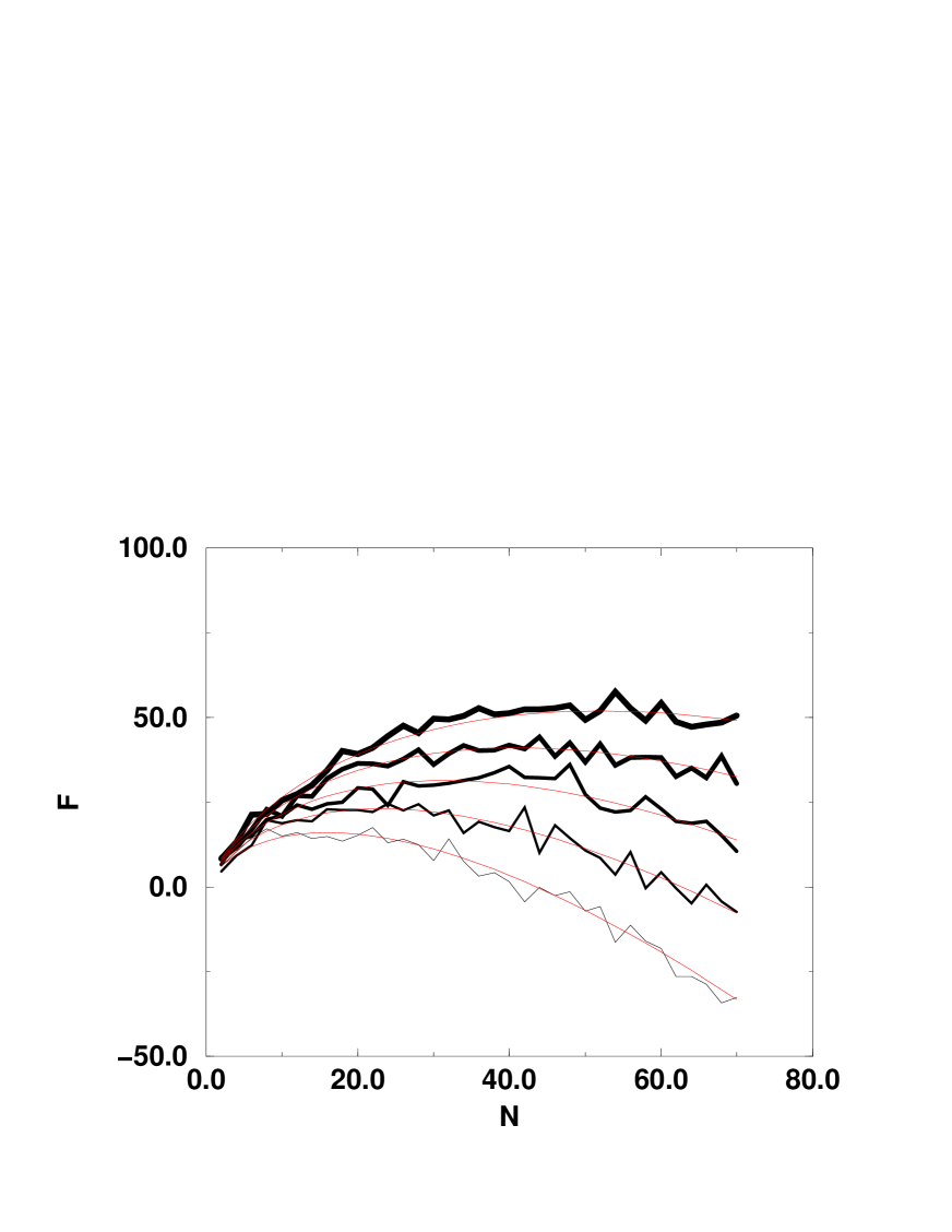
Figure 5: Density of the Coulomb gas ($N_{c}=2$): The curves in the figure show the free energy $F$ versus the number of instantons $N$ using 20.000 Metropolis steps until equilibrium is reached. From thin to bold we use the lengths $L=0.5$, $L=0.6$, $L=0.7$, $L=0.8$, and $L=0.9$. The smooth solid curves show the combined fit with the scaling function $F(L,N)=N[\ln(L^{2})-(\ln(N)-1-\ln(n_{+}))]+a$, with a single $a$ and $n_{+}$ given to fit all five curves simultaneously. If we fit each curve separately we get from thin to bold the following values for the density $n_{+}=62.341$, $n_{+}=64.526$, $n_{+}=66.027$, $n_{+}=63.857$, and $n_{+}=63.836$. In case of the combined fit we get for the density the value $n_{+,{\rm best}}=64.117\pm 1.193$, where the error is the standard deviation derived from the five separate measurements of $n_{+}$ given above. The cutoff parameter in this figure is ${\epsilon^{\prime}}^{2}=0.001$. The defect $\alpha$ is 0.481.

The first question is whether this system has a thermodynamic equilibrium, i.e. whether its density does not change with the system volume $L^{2}$, when $L$ is large. We start again with the Coulomb gas of two noninteracting ensembles of instantons and anti-instantons, i.e. $(\beta_{1}=0)$ and $N_{c}=2$. Here it is sufficient to consider the instantons alone. In this case we simply have $N=N_{+}$ and we plot the logarithm of the partition function, i.e. the free energy as a function of the number of instantons $N$. The ideal situation would be now that the number $N_{\rm max}$, where the partition function has a maximum, is proportional to $L^{2}$. Then one could continue this situation to an infinite instanton ensemble with the same density. In Fig. 5 we show the partition function for the Coulomb gas as a function of the number of instantons $N$ for various box lengths $L$. The simulation is done with the UV cutoff $\epsilon^{\prime 2}=0.001$. One sees that the free energy is plagued by large fluctuations that correspond to fluctuations in orders of magnitude in the partition function. A direct determination of the maximum of the free energy is not reliable. Instead, one can exploit the expected scaling behavior. If the system has a stable density then the free energy must be of the form:

$$F(\epsilon^{\prime},N,L)=\ln Z(\epsilon^{\prime},N,L)=N\{\ln(L^{2})-[\ln(N)-1-\ln(n_{+}(\epsilon^{\prime}))]\}+a\;,$$ (58)

with the two fit constants $a$ and $n_{+}(\epsilon^{\prime})$, and $\epsilon^{\prime}=\epsilon/L$ being fixed in order to preserve the scaling behavior of the initially unregularized theory. Eq. (58) is obtained in the following way: From the inspection of Eq. (37) it is clear that the free energy depends on $L$ via $N\ln(L^{2})$. Requiring now that the number $N$ at the maximum of the free energy $F$ is proportional to $L^{2}$ leads to a differential equation with the solution given by Eq. (58). Eq. (58) has the advantage that $n_{+}(\epsilon^{\prime})$ gives immediately the density of the system. The symbol $n_{+}$ refers to the instanton density. Unfortunately, the system does not exhibit a stable density. The reason is, again, the tendency of the system to condense into neutral pairs corresponding to small-size instantons. When it happens, it is not reasonable anymore to write down the particle-identity factor $1/(N!)^{2}$ in the partition function: it should be rather replaced by the first power of the factorial. Therefore, we allow for an additional ‘conbinatorical defect’ term in the fit, which reads $\alpha\ln N!$, so that the full fit function has now the form:

$$F_{\rm fit}(\epsilon^{\prime},N,L)=N\{\ln(L^{2})-[\ln(N)-1-\ln(n_{+}(\epsilon^{\prime}))]\}+\alpha\ln N!+a\;.$$ (59)

The smooth solid lines in Fig. 5 are the fitted curves, which fit quite well to the heavily fluctuating free energy. One should expect that the defect becomes smaller when $\epsilon^{\prime}$ becomes smaller. As shown in Tab. 1, one sees indeed such a behavior.

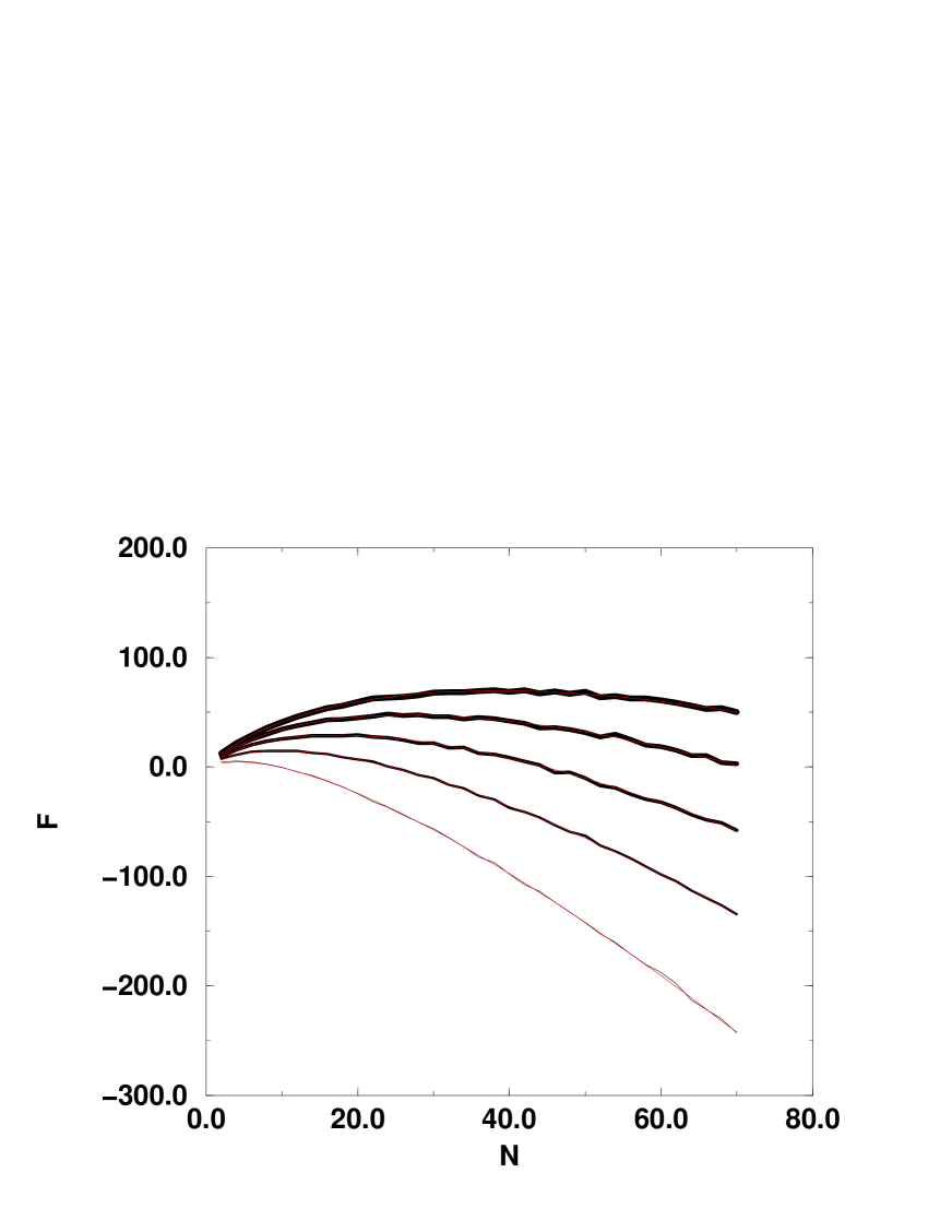
Figure 6: Check of the Debye-Hückel approximation to the Coulomb gas ($N_{c}=2$). The solid lines from thin to bold give the measured value for a Coulomb gas with $\beta=0.1$ and lengths $L=2,L=3,L=4,L=5,L=6$. The thin smooth solid lines show the prediction of the scaling law, which is F(N,L) = $(2-\beta)N[\ln(L^{2})-(\ln(N)-1-\ln(n_{+}))]+a$, where $N$ in this case is the number of instantons only, as we do not consider any anti-instantons here. The four curves yield the value for $n_{+}=1.06787\pm 0.0024$, which is in agreement with the prediction of the Debye-Hückel approximation, which gives $n_{+,\rm Debye}=1.0370$.

Now arises the question how reliable our simulations are, because so far we did not find strictly speaking a stable system. The situation is also not very comfortable because in the limit $\epsilon^{\prime}=0$, where a stable phase should exist the density $n_{+}$ is divergent for $N_{c}=2$. We therefore study now a different regularization method: It consists in introducing a temperature $T=1/\beta$ in the zindon interactions, with $\beta<1$. We reach the physical limit by taking $\beta\rightarrow 1$. For small values of $\beta$ we expect behavior of the system to be consistent with the predictions of the Debye-Hückel approximation. In Fig. 6 we show the free energy for $\beta=0.1$ versus the number of instantons $N$. The solid lines are the fits using the form:

$$F_{\rm fit,\;Debye}(N,L)=N\{\ln(L^{2})-[\ln(N)-1-\ln(n_{+,{\rm Debye}})]\}+a\;.$$ (60)

We find a stable density for various box lengths $L$. The five curves yield a value for $n_{+}=1.06787\pm 0.0024$, which is in agreement with the prediction of the Debye-Hückel approximation: (55) gives $n_{+,{\rm Debye}}=1.0370$.

We now switch on the interaction between instantons and anti-instantons putting $\beta_{1}>0$. Again we can only determine a kind of stable density $n_{+}(\epsilon^{\prime})$, if we allow for a defect parameter. Tab. 2 shows the results for $n_{+}(\epsilon^{\prime})$ for three different values of $\epsilon^{\prime}$ as a function of $\beta_{1}$. In case of $\beta_{1}=0$ we can compare the density to the one in Tab. 1, both are results of independent simulations. A comparison of the upper line in Tab. 2 with corresponding entries in Tab. 1 gives an idea of the statistical error; it is not enormous, but certainly not negligible.

We observe that the density rises only slowly with $\beta_{1}$. This is in agreement with the results of the Debye-Hückel approximation, which also predicts a slow rising of the density with $\beta_{1}$. For $N_{c}=2$, the equilibrium density is given by (see Eq. (55)):

$$n_{+}=\frac{1}{2}\Bigg{[}f(\beta_{1})\pi\beta e^{2\gamma_{E}}2^{\frac{2}{\beta}}\Bigg{]}^{\frac{\beta}{2-\beta}};\quad f(\beta_{1})=(1+\beta_{1})^{\frac{1+\beta_{1}}{2}}(1-\beta_{1})^{\frac{1-\beta_{1}}{2}}\;.$$ (61)

The function $f(\beta_{1})$ varies between 1 and 2 for $\beta_{1}$ varying between 0 and 1. For the real $CP^{1}$ model, when $\beta=1$, we can expect at least a behavior linear in $\ln f(\beta_{1})$ for the logarithm of the density $\ln n_{+}$. Fig. 7 shows, indeed, that we can obtain a good linear fit, using this assumption. The numerical results for the linear fit can be read off from Tab. 3. The growth of the intercept $a$ when ${\epsilon^{\prime}}^{2}$ goes to zero reflects the fact that in this theory the density is divergent. The growth of the slope $b$ is also natural, since at $\epsilon^{\prime}\rightarrow 0$ we expect $b=1$ from Eq. (61). In general one sees that the effect of the instanton–anti-instanton coupling on the density is comparatively small as predicted also by the Debye-Hückel approximation.

Finally, let us discuss the running of the instanton–anti-instanton coupling $\beta_{1}$. From its derivation in Sec. 3.2 it is seen that $\beta_{1}=\pi/g^{2}$ ( at $N_{c}=2$) is related to the bare coupling constant of the theory $g^{2}$. However, physical quantities cannot depend on the bare couplings, but only on the renormalized ones. It means that by considering quantum corrections to the classical instanton–anti-instanton interactions one would be able to observe that the bare coupling constant $g^{2}$ (or $\beta_{1}$) is replaced by the running coupling depending on the characteristic scale in the problem at hand. In our case the only dimensional scale is the average separation between instantons and anti-instantons or, else, the density of zindons, $n$. From renormalization-group arguments one can write the 1-loop formula

$$\beta_{1}=\frac{1}{2}\left(\ln\frac{N}{L^{2}}+C\right)\;,$$ (62)

however, the constant $C$ remains unknown. In order to determine $C$ one has to perform the renormalization of the instanton–anti-instantons interaction with a very high precision; this has not been done. 

Keeping in mind that the dependence of the instanton density on $\beta_{1}$ is very mild in the whole range $0<\beta_{1}<1$ (see Fig. 7 and Tab. 2) and that the dependence of $\beta_{1}$ on the density is also quite weak (see (62)), and given the theoretical uncertainty in the constant $C$, we cannot reliably determine the density self-consistently by taking into account the running of $\beta_{1}$. In the case of $N_{c}=2$ by far a more important factor affecting the density is the necessary ultraviolet cutoff $\epsilon$.

6.2 The case $N_{c}=3,4$

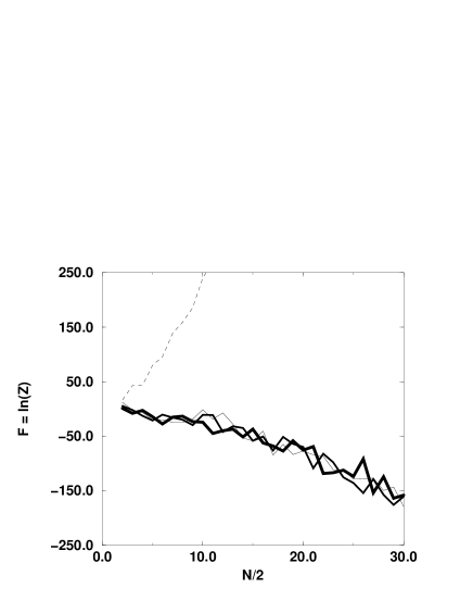
Figure 8: Free energy versus the number of instantons (equal to the number of anti-instantons), $N/2=N_{-}=N_{+}$. The figures show the free energy versus $N/2$ for $N_{c}=3$ (on the left) and $N_{c}=4$ (on the right). The solid lines from thin to bold are for $\beta_{1}=0.0$, $\beta_{1}=0.2$, and $\beta_{1}=0.4$. The dashed line is the free energy for the value $\beta_{1}=1$, which shows all signs of a collapse.

In the case $N_{c}=3,4$ we are not plagued with the necessity to introduce a regulator. However, we are confronted now with enormous fluctuations. In Fig. 8 the free energy is plotted for several values of $\beta_{1}$. Already in the free energy the fluctuations are of an order of magnitude, so that a reasonable determination of the equilibrium density is not possible. However, we could at least try to compare the situation to the one in the Debye-Hückel approximation for $N_{c}=3,4$. First of all it is necessary to mention that our partition function (37) is not based on two-body interactions only, and is therefore not directly comparable to the one used to derive the density (55). But, as we will see now, some of the features are nevertheless strikingly in parallel. First of all it turns out that for all values of $\beta_{1}$ not too close to the critical value, the free energy does not change much (as compared to the extremely large fluctuations). This is in parallel to the fact that the equilibrium density given by the Debye-Hückel approximation grows only slowly with $\beta_{1}$, see Fig. 9. Another feature of the Debye-Hückel result for the equilibrium density is that it is comparatively large for $N_{c}=2$ and then falls rapidly to the asymptotic value $n_{+}(N_{c}=\infty,\beta=1,\beta_{1}=0)=\pi^{1/7}\exp(2\gamma_{E}/7)\approx 1.3888$. The second point, where there is something in parallel between the Debye-Hückel result and the simulations, concerns the critical behavior. The Debye-Hückel formula for the density becomes meaningless when $\beta_{1}\geq N_{c}/2(N_{c}-1)$. Hence for $N_{c}=3$ we find $\beta_{\rm crit}=3/4$ and for $N_{c}=4$ we find $\beta_{\rm crit}=2/3$. In the simulations it is seen (Fig. 8) that for values of $\beta_{1}\simeq 1$ the system behaves abnormally and shows clear signs of a collapse.

7 Size distribution

A very important question is what is the size distribution of instantons in the ensemble. Is the average size $\langle\rho\rangle$ smaller or larger than the average separation between instantons $\langle R\rangle=n^{-1/2}$? In the former case one can say that instantons are dilute while in the latter case one says that instantons ‘melt’, so that individual instantons have not much sense.

We are now in a position to study this problem quantitatively. The zindon parametrization of instantons is an ideal tool for that since it allows for both extreme cases. If zindons of different ‘color’ are uniformly distributed in space that would mean the instantons ‘melt’. If zindons of $N_{c}$ colors tend to form well-isolated color-neutral clusters, it means instantons are dilute. The size distribution of instantons has been measured on the lattice for $N_{c}=2$ [14] after a cooling procedure has been applied to remove short-range fluctuations. (For a recent comparison of different cooling techniques on the $CP^{N_{c}-1}$ model see also [22].) A very delicate question in connection to this is, how to identify instantons on the lattice. Several procedures are in use [1]. In this paper we want to compare two ways of extracting the instanton content. The first one, which we call the ‘geometric’ method, makes use of the zindon picture. From the sample of all zindons the color neutral $N_{c}$-plet which has the least dispersion about the common center is chosen to be an instanton. Then all zindons belonging to this instanton are removed from the sample, and the procedure is iterated to find the next group of zindons that has the smallest dispersion and so on, until the whole sample is grouped into instantons. The second procedure, which we call the ‘lattice’ method as it is more close to the ones used in lattice studies, is looking for local maxima of the topological charge density $q(x)$ on a $N_{\rm grid}\times N_{\rm grid}$ lattice. An instanton is assumed if a grid point has a larger topological charge than its surrounding 8 nearest neighbors. In order to improve the accuracy in finding the center points and the sizes, we construct an interpolating polynomial,

$$q(x,y)=ax^{2}y^{2}+bx^{2}y+cxy^{2}+dx^{2}+ey^{2}+fxy+gx+hy+j,$$ (63)

calculated from the 9 grid points consisting of the grid point under consideration and its 8 neighbors. From this interpolating function we find coordinates of the local extrema $x_{E}$. An extremum is accepted if it lies inside the $3\times 3$ grid used for the interpolation. In order to classify whether we have found a local maximum, minimum or a saddle point we construct the matrix of second derivatives at the extremum $x_{E}$:

$$\left(\begin{array}[]{cc}\left(\frac{\partial}{\partial x}\right)^{2}&\frac{\partial}{\partial x}\frac{\partial}{\partial y}\\ \frac{\partial}{\partial x}\frac{\partial}{\partial y}&\left(\frac{\partial}{\partial y}\right)^{2}\\ \end{array}\right)q(x_{E})\;.$$ (64)

If the two eigenvalues $\lambda_{1}$ and $\lambda_{2}$ of this matrix have a different sign then $x_{E}$ is a saddle point and is rejected. For negative $\lambda_{1}$ and $\lambda_{2}$ we have a local maximum and respectively a local minimum if both $\lambda_{1}$ and $\lambda_{2}$ are positive. The two eigenvalues give at the same time a measure for the size $\rho_{i}^{2}=\sqrt{8/|2\pi\lambda_{i}|},\;i=1,2$ (they should coincide for an ideal spherically-symmetric instanton). This size can be compared to the one derived from the value of the topological charge at the maximum $\rho_{3}^{2}=2/|2\pi q(x_{E})|$. Only if all three sizes are smaller than $L/2$ is the instantons or anti-instanton accepted and the size is then taken to be the geometrical mean of the three definitions, $\rho=(\rho_{1}\rho_{2}\rho_{3})^{1/3}$. It should be noted that usually $\rho_{1,2,3}$ are not drastically different. We should also stress that a reliable identification of all local extrema is achieved only with a fine grid. With a 100$\times$100 grid we find almost the same number of maxima (instantons) and minima (anti-instantons) as we put in ‘by hands’ by fixing the number of zindons and anti-zindons.

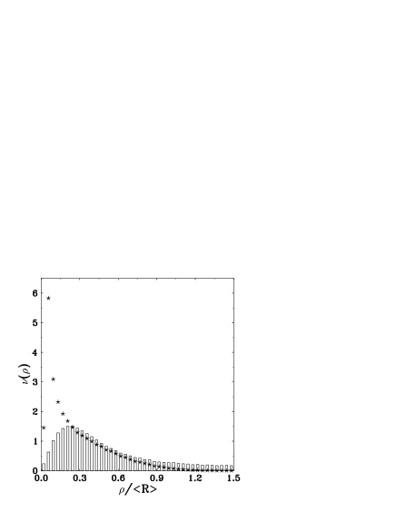
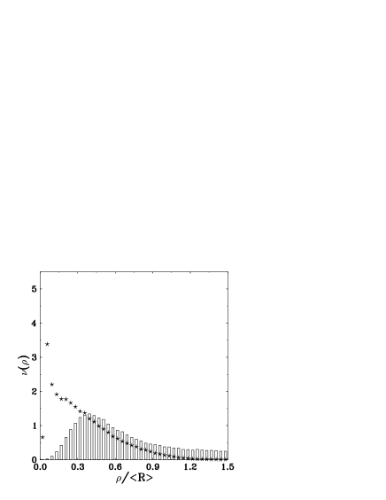
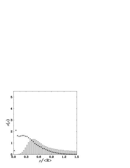
Figure 10: Instanton size distribution following from random (non-interacting) zindons are displayed for $N_{c}=2$ (on the top), $N_{c}=3$ (bottom left), and $N_{c}=4$ (bottom right) for $N_{+}=N_{-}=8$. The histograms show the size distributions ‘geometrically’ defined by grouping zindons according to their dispersion $\rho$. The stars show the result for the ‘lattice’ method using a $100\times 100$ grid.

We first test both methods, the ‘geometric’ and the ‘lattice’, in a toy model where the positions of zindons and anti-zindons are random: the interactions are switched off completely ($\beta=0$ and $\beta_{1}=0$) so that the distribution of zindons in space is given by a flat measure $\prod d^{2}a_{Ai}\prod d^{2}b_{Aj}$. We generate configurations of zindons with this measure and compute the topological charge density $q(x)$ of a given configuration from the integrand of Eq. (14). Instantons and anti-instantons are then identified by the two methods described above. Taking many configurations we compute the distribution of the instanton sizes, see Fig. 10.

For the flat measure the small-$\rho$ side of the distribution can be immediatelly evaluated from dimensions to be $\nu(\rho)\sim\rho^{2N_{c}-3}$. The geometric distribution (shown by histograms) follows this prediction whereas the lattice method strongly deviates from it. [One can mimic the smooth geometric distribution by the lattice method by taking a crude grid but then many instantons are lost as they “fall through” the grid.] The fact is that the topological density computed from randomly distributed zindons shows many sharp and narrow peaks. The larger number of instantons we take (at fixed density) the more sharp the peaks become: it clearly indicates a non-thermodynamic behavior of the system.

This pathological behavior is due to the utmost instability of the product Ansatz (13) in the case when the interactions are swithched off. Indeed, the sizes of instantons are determined by Eq. (18) where the role of the weights $c_{A}$ is played by long products (19). These products are extremely unstable: sufficient to change the positions of very distant zindons, and $c_{A}$’s will change. With zindons distributed according to the flat measure $c_{A}$’s fluctuate by orders of magnitude, and the more zindons are taken the stronger they fluctuate. It means that there will always be a zindon of a certain color whose weight $c_{A}$ is much much larger than those of the other zindons forming an instanton. According to Eqs.(17, 18) the extremum of the topological density will then coincide with the position of the zindon of that particular color, and the size of the corresponding instanton will be close to zero. This is why we see too many small-size instantons by the lattice method. See also the discussion around Fig. 12 below.

When we switch on the interactions zindons get correlated and the product Ansatz should not be pathological any more. In particular, from the experience of the Debye–Hückel approximation we know that the correlation functions of zindons get exponentially suppressed at large separations. Therefore, we expect that the topological density will not have unphysical sharp peaks at small $\rho$ as in the case of the flat measure, and the two methods of instanton identification should come closer. In practice, however, one cannot be sure beforehand that the thermodynamic equilibrium is fully reached, given the limited computer time for configuration generation.

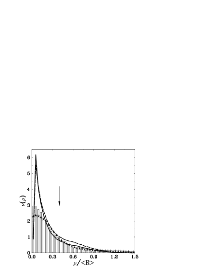
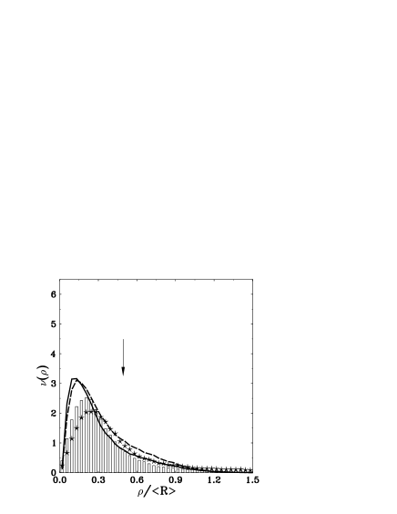
Figure 11: Instanton size distributions with zindon interactions switched on are displayed for $N_{c}=3$ (left), and $N_{c}=4$ (right) for $N_{+}=N_{-}=8$. The histograms show the ‘geometric’ size distributions, and the solid lines the size distributions seen by the ‘lattice’ method, again using a $100\times 100$ lattice. The instanton–anti-instanton coupling constant for the solid lines and the histograms is $\beta_{1}=0.0$. The stars and the dashed lines show the ‘geometric’ and ‘lattice’ size distributions for the case of $\beta_{1}=0.5$. Instanton sizes are plotted in units of the average separation $\langle R\rangle$. The arrows show the maxima of the corresponding ‘geometric’ size distributions obtained in the non-interacting case of Fig. 10.

We switch on the interactions, first, only of zindons belonging to same-kind instantons ($\beta_{1}=0$) and then adding interactions between instantons and anti-instantons ($\beta_{1}=0.5$), see Fig. 11. We show only the cases $N_{c}=3,4$ as for $N_{c}=2$ the size distribution is cutoff dependent. For the ‘lattice’ method we use again the $100\times 100$ grid. Unfortunately, the fluctuations of the partition function in the simulations are so large that we have to apply a trick in order to get meaningful results. We let the Metropolis algorithm work until a plateau is reached. Then we make many measurements of the size distribution at the plateau, all weighted with a weight averaged over the plateau. We repeat this for several starts but we essentially see the size distribution for the plateau possessing the largest free energy.

The price we have to pay for this somewhat truncated simulation is that the unphysical peaks at small $\rho$, as determined from the lattice method, are still present though they are not so awkward as in the non-interacting case. As $N_{c}$ increases the small-$\rho$ peak shrinks, therefore one can speculate that at large $N_{c}$ it is easier to reach the thermodynamic equilibrium. Except for very small $\rho$ the two methods of instanton identification seem to produce rather similar distributions.

The geometric size distribution exhibits the expected behavior at all $\rho$. In particular, at small $\rho$ it behaves as $\nu(\rho)\sim\rho^{b-3}$ where $b=N_{c}$ is the 1-loop Gell-Mann–Low coefficient, which is to be expected from dimensional analysis.

We observe that the instanton–anti-instanton interaction does not influence the size distributions significantly. This is seen both from geometric and lattice methods by comparing curves in Fig. 11 with $\beta_{1}=0$ and $\beta_{1}=0.5$. The case $\beta_{1}=0.5$ has a slightly broader distribution. Qualitatively, it should be anticipated since the interactions between zindons and anti-zindons tend to ‘pull out’ individual zindons out of their neutral clusters, however, the effect is small.

As to the interactions of the same-kind zindons, it clearly leads to smaller instanton sizes; this could be also anticipated. Indeed, the zindon interactions are such that same-color zindons are repulsive while different-color zindons are, on the average, attractive. Such interactions lead to preferred clustering of zindons into color-neutral groups. (This is especially clear for $N_{c}=2$ where the Coulomb interaction leads, as we have seen, to a collapse of zindons into neutral pairs as one removes the ultraviolet cutoff, $\epsilon\rightarrow 0$). In Fig. 11 we show by arrows at the top of the plots the positions of the ‘geometric’ distributions maxima in the non-interacting case of Fig. 10: both for $N_{c}=3$ and 4 the maxima are noticeably shifted to smaller sizes when one switches on the interactions. The ‘lattice’ method shows this shift only in the case $N_{c}=4$ where the unphysical small-size peaks of the topological density are suppressed.

In Fig. 12 we plot the topological density obtained from a typical configuration of zindons at $N_{c}=3$ with all interactions taken into account. We see that the peaks of the topological density in general correlate with the positions of the centers of instantons found by the ‘geometric’ method (shown by triangles in Fig. 12). In some cases, however, the peaks of the topological charge density sit not in the centers of the 3-plet of zindons forming an instanton but rather near one of the three zindons. This is the consequence of the instability of the weight coefficients $c_{A}$, discussed above, and is the actual cause of the small-$\rho$ peaks in the ‘lattice’ size distributions.

Finally, we would like to draw attention to the fact that in Fig. 11 we have plotted the instanton sizes in units of the average separation between instantons, defined as $\langle R\rangle=(N/V)^{-1/2}$. It is remarkable that both for $N_{c}=3$ and 4 and independently of the method used to identify instantons, the average instanton size is definitely smaller than the average separation. It means that instantons formed of $N_{c}$-plets of zindons are, on the average, dilute. Though one can always find a huge instanton overlapping with many others, the probability of such an event is relatively low.

8 Conclusions

We have formulated the statistical mechanics of instantons and anti-instantons in the $d=2$ $CP^{N_{c}-1}$ models in terms of their ‘constituents’ which we call ‘zindons’. We have derived the interactions of same-kind and opposite-kind zindons for arbitrary $N_{c}$. At $N_{c}=2$ they come to logarithmic Coulomb interactions known previously. At $N_{c}>2$ the interactions are of a many-body type though one can reasonably approximate them by two body logarithmic interactions with charges depending on the ‘color’ of zindons.

At high temperatures the system can be studied analytically by ways of the Debye-Hückel approximation, at any $N_{c}$. The physical case corresponds to the temperature $\beta=1$ and can be studied by a Metropolis-type simulation. The numerical study shows that the Debye-Hückel approximation is, as expected, accurate at small $\beta$, but is qualitatively valid even at $\beta=1$. Both analytical an numerical studies indicate that the effect of instanton–anti-instanton interactions (in our language the zindon–anti-zindon interactions) is not significant: the interaction of same-kind zindons or, else, the multi-instanton measure, is by far more important for the statistical mechanics of the instantons–anti-instanton ensemble.

At $N_{c}=2$ the system is, strictly speaking, collapsing into instantons of zero size: to regularize its behavior one needs to introduce an ultraviolet cutoff. We have studied in detail the statistical mechanics with varying cutoff parameter: the numerical simulations are fully compatible with the expectations.

At $N_{c}=3,4$ the system does thermodynamically exist with no cutoff, however, it exhibits enormous fluctuations which undermine accurate measurements of physical quantities. Nevertheless, we have managed to study the instanton size distribution introducing two methods of its determination, ‘geometric’ and ‘lattice’. Using the ‘lattice’ method with a very fine grid we observe many unphysical small size instantons for $N_{c}=3$, which stem from the instability of the product Ansatz. Though this effect is believed to disappear when the system approaches the true statistical equilibrium it is very difficult to get rid of it in practice because of gigantic fluctuations in the system. The effect is even more pronounced for the flat measure but tends to vanish when $N_{c}$ is increased.

Though the zindon parametrization of instantons and of their interactions allows for complete ‘melting’ of instantons and is quite opposite in spirit to dilute gas Ansätze, we observe that zindons, nevertheless, tend to form ‘color-neutral’ clusters which can be identified with well-isolated instantons. This effect is due to a combination of two different factors both supporting clustering. One factor is the interactions: same-color zindons are strongly repulsive while different-color zindons are attractive. The second factor is pure geometry: even with a flat measure the probability to combine $N_{c}$ zindons into a neutral cluster smaller than the average separation is quite sizeable. Both these factors are expected to be even stronger in four dimensions appropriate for the Yang-Mills instantons.

Acknowledgments
Stimulating discussions with Dima Khveschenko, Alan Luther and especially with Victor Petrov are gratefully acknowledged.

${\epsilon^{\prime}}^{\prime 2}$	density $n_{+}$	average distance $1/\sqrt{n_{+}}$	$L_{\rm max}$	$N_{\rm max}$	defect $\alpha$
0.1	5.095 $\pm$ 0.021	0.443	1.401	10	0.839
0.03	12.707 $\pm$ 0.107	0.281	1.620	33	0.777
0.01	23.501 $\pm$ 0.211	0.206	2.063	100	0.672
0.003	42.723 $\pm$ 0.673	0.153	2.793	333	0.571
0.001	64.117 $\pm$ 1.193	0.125	3.949	1000	0.481
0.0003	135.207 $\pm$ 4.299	0.086	4.965	3333	0.518

Table 1: Dependence of the zindon density in the Coulomb gas on the cutoff parameter. The error is given by the standard deviation of the $n_{+}$’s obtained by separate fits to five measured curves. The value of $n_{+}$ itself is the value one obtains if one performs a combined fit with one $n_{+}$ to all the measured curves. The real value of $n_{+}$, however, is determined by the error in the defect $\alpha$, to gain experience of its influence one may compare to Tab. 2.

$\beta_{1}$	${\epsilon^{\prime}}^{2}=0.1$	${\epsilon^{\prime}}^{2}=0.01$	${\epsilon^{\prime}}^{2}=0.001$
	$\alpha=0.7539$	$\alpha=.5785$	$\alpha=0.45992$
	$(A=-0.036$)	$(A=-0.035)$	$A=-0.013$
0.0	6.946	26.314	74.948
0.1	7.062	27.614	75.371
0.2	6.945	27.650	75.250
0.3	7.060	28.229	74.075
0.4	7.080	27.711	81.660
0.5	7.164	27.707	77.512
0.6	7.006	29.171	80.946
0.7	7.149	28.706	82.323
0.8	7.306	30.013	91.595
0.9	7.395	31.705	93.606
1.0	7.624	34.757	119.714

Table 2: Dependence of the instanton density $n_{+}$ on the coupling parameter $\beta_{1}$. In the table the density $n_{+}$ is given for three different values of ${\epsilon^{\prime}}^{2}$ ($L=1$). One should note that the defect $\alpha$ has quite a large error, therefore the resulting values for the density at $\beta_{1}=0$ are different from the one in Tab. 1 due to this statistical error. $A$ is the intercept from the combined fit of the free energy to a form $F=A+N[\ln(N/L^{2})-1]+N\ln n+\alpha\ln N!$ and it is a small quantity, which can be neglected in the further discussion.

${\epsilon^{\prime}}^{2}$	$a$	$b$
0.1	1.94273	0.119835
0.01	3.29677	0.331814
0.001	4.29687	0.607095

Table 3: Fit of the equilibrium density to the form given by the Debye-Hückel approximation. The table shows the results for the linear fit to the form $\ln n_{+}=a+b\ln f(\beta_{1})$, where $\ln f(\beta_{1})=\frac{1}{2}[(1+\beta_{1})\ln(1+\beta_{1})+(1-\beta_{1})\ln(1-\beta_{1})]$. The increase of the intercept when ${\epsilon^{\prime}}^{2}$ becomes smaller is due to the fact the the density for $N_{c}=2$ is divergent. All values are for $\beta=1$.

Figure 1: The ‘dilute’ regime for $N_{c}=3$: Concentrating around the center-of-mass points $x_{1}$, $x_{2}$, and $x_{3}$ zindons of three different colors are closely grouped together to form instantons with large distances $R_{ij}$ between them. The configuration corresponds to a dilute gas of non-overlapping instantons.

Figure 2: Stability of the Metropolis algorithm for $N_{c}=2$ [${\epsilon^{\prime}}^{2}=0.001$] (on the left) and $N_{c}=3$ (on the right, bold line) $N_{c}=4$ (on the right, thin line). The graphs show the free energy improved step by step by the Metropolis algorithm until a plateau of ‘important’ configurations is reached. In all three runs we used $N_{+}=30$ and $L=10$. In all cases the interaction between instantons and anti-instantons is switched off $(\beta_{1}=0)$.

Figure 3: Snapshots of zindon configurations at the plateau after 500.000 Metropolis steps: The figure shows the spatial distribution of zindons for $N_{c}=2$ (on the top ), $N_{c}=3$ (bottom left) and $N_{c}=4$ (bottom right). The filled and empty circles and squares symbolize different colors. Only for $N_{c}=2$ a condensation into neutral pairs is observed; for higher $N_{c}$ the free energy is finite though many distinct ‘color-neutral’ $N_{c}$-plets are seen. Only instanton-zindons are shown.

Figure 4: Divergent/convergent behavior of the free energy: The free energy is plotted versus $\ln(\ln(100/\epsilon))$ for $N_{c}=2$ (top), $N_{c}=3$ (bottom left), and $N_{c}=4$ (bottom right). One observes a divergent behavior for $N_{c}=2$, while the free energy is finite for $N_{c}=3$ and $N_{c}=4$. The last point in the plots with $N_{c}=3$ and $N_{c}=4$ is calculated using $\epsilon=0$.

Figure 7: Fit of the equilibrium density to the form given by the Debye-Hückel approximation. According to the Debye-Hückel approximation the logarithm of the density $\ln n_{+}$ is linear in $\ln f(\beta_{1})$, where $\ln f(\beta_{1})=\frac{1}{2}[(1+\beta_{1})\ln(1+\beta_{1})+(1-\beta_{1})\ln(1-\beta_{1})]$. In the figure the data for $\ln n_{+}$ are shown versus $\ln f(\beta_{1})$, where the triangles belong to the sample with ${\epsilon^{\prime}}^{2}=0.1$, the squares to the sample with ${\epsilon^{\prime}}^{2}=0.01$ and the circles to the sample with ${\epsilon^{\prime}}^{2}=0.001$. The solid lines are linear fits. The corresponding fit constants are given in Tab. 3.

Figure 9: Prediction of the Debye-Hückel approximation for the density at $\beta=1$. The solid line is the Debye-Hückel prediction for $N_{c}=2$, the dotted line for $N_{c}=3$, the dashed-dotted line for $N_{c}=4$, and the dashed line shows the limit $N_{c}\to\infty$. The lines end at critical couplings.

Figure 12: Topology of a sample with 3 instantons and 3 anti-instantons ($N_{c}=3$) seen by the ‘lattice’ method. The sample has been generated with the full partition function at the plateau for $\beta_{1}=0.5$. On the left we show the the zindon content of the configuration. The triangles connect zindons of three different colors forming instantons (solid lines) and anti-instantons (dashed lines), as found by the ‘geometric’ method. Filled symbols correspond to zindons, open symbols to anti-zindons. The diamonds, squares and triangles denote the different colors. The stars show the centers and the circles show instanton sizes, as found by the ‘lattice’ method using a $100\times 100$ grid. The method has been applied to the topological charge density displayed as a 3-dimensional plot on the right.

References

- [1] J. W. Negele, Nucl. Phys. Proc. Suppl. 73, 92 (1999).
- [2] T. Schaefer and E. Shuryak, Rev. Mod. Phys. 70, 323 (1998).
-
[3]
D. I. Diakonov, V. Yu. Petrov, Nucl. Phys. B 272, 457 (1986),
D. Diakonov, in: Selected Topics in Non-perturbative QCD, Proc. Enrico Fermi School, Course CXXX, A. Di Giacomo and D. Diakonov, eds., Bologna, (1996) p.397, hep-ph/9602375. - [4] V. L. Golo and A. M. Perelomov, Phys. Lett. B 79, 112 (1978).
- [5] A. D’Adda, M. Luescher and P. Di Vecchia, Nucl. Phys. B 146, 63 (1978).
- [6] V. Fateev, I. Frolov and A. Schwartz, Nucl. Phys. B 154, 1 (1979).
- [7] V. Fateev, I. Frolov and A. Schwartz, Sov. J. Nucl. Phys. 30(4), 590 (1979).
- [8] B. Berg and M. Lüscher, Comm. Math. Phys. 69, 57 (1979).
- [9] E. Witten, Nucl. Phys. B 149, 285 (1979).
- [10] L. D. Faddeev, N. Yu. Reshetikhin, Annals Phys. 167, 227 (1986).
- [11] M. Campostrini, A. Pelissetto, P. Rossi, E. Vicari Phys. Rev. D 54, 1782 (1996).
- [12] M. Campostrini, P. Rossi, E. Vicari, Phys. Rev. D 46, 4643 (1992).
- [13] A. Di Giacomo, F. Farchioni, A. Papa, E. Vicari, Phys. Rev. D 46, 4630 (1992).
- [14] C. Michael, P. S. Spencer, Phys. Rev. D 50, 7570 (1994).
- [15] A. P. Bukhvostov and L. N. Lipatov, Nucl. Phys. B 180, 116 (1981); Pisma Zh. Eksp. Teor. Fiz. 31, 138 (1980).
- [16] A. A. Belavin, A. M. Polyakov, JETP Lett. 22, 245 (1975); Pisma Zh. Eksp. Teor. Fiz. 22, 503 (1975).
- [17] D. Diakonov and V. Petrov, Towards a New Formulation of the Yang–Mills Theory, report PNPI-90-1581 (1990), unpublished.
- [18] A. Jevicki, Nucl. Phys. B 127, 125 (1977).
- [19] L. D. Landau and E. M. Lifshitz, Statistical Physics, chapter VII,p. 74, Pergamon Press, London-Paris, 1958.
- [20] A. Jevicki, Phys. Rev. D 20, 3331 (1979).
- [21] A. Polyakov, Gauge Fields and Strings, Harwood Academic Publishers, 1987.
- [22] B. Alles, L. Cosmai, M. D’Elia, A. Papa, Topology in the models: a critical comparision of different cooling techniques, BARI-TH-355-99, Sep 1999. 3pp., e-Print Archive: hep-lat/9909034.