Three loop renormalization of the $SU(N_{c})$ non-abelian Thirring model

Abstract. We renormalize to three loops a version of the Thirring model where the fermion fields not only lie in the fundamental representation of a non-abelian colour group $SU(N_{\!c})$ but also depend on the number of flavours, $N_{\!f}$. The model is not multiplicatively renormalizable in dimensional regularization due to the generation of evanescent operators which emerge at each loop order. Their effect in the construction of the true wave function, mass and coupling constant renormalization constants is handled by considering the projection technique to a new order. Having constructed the $\overline{\mbox{MS}}$ renormalization group functions we consider other massless independent renormalization schemes to ensure that the renormalization is consistent with the equivalence of the non-abelian Thirring model with other models with a four-fermi interaction. One feature to emerge from the computation is the establishment of the fact that the $SU(N_{\!f})$ Gross Neveu model is not multiplicatively renormalizable in dimensional regularization. An evanescent operator arises first at three loops and we determine its associated renormalization constant explicitly.

LTH-456

1 Introduction.

Models with a four-fermi interaction have played an important role in exploring fundamental properties of physical quantum field theories. For example, the two dimensional $O(N)$ Gross Neveu model, [1], is similar to QCD in that it is asymptotically free. Another two dimensional four-fermi theory which shares similar properties to the Gross Neveu model is the Thirring model with a non-abelian symmetry, [2]. It too is asymptotically free and additionally is more closely related to QCD itself. For instance, when the fermion fields of the non-abelian Thirring model, (NATM), have the same quantum numbers as the quarks of QCD, with $N_{\!f}$ flavour dependence in addition to being in the fundamental representation of the colour group, it has been argued that it is equivalent to QCD in the large $N_{\!f}$ limit, [3]. More precisely, Hasenfratz and Hasenfratz demonstrated that by taking the NATM in its $d$-dimensional extension then integrating over the leading quark loops which dominate when $N_{\!f}$ is large, the usual three and four gluon vertices of QCD are recovered as one approaches four dimensions. Moreover, graphs with a quark loop and five or more external gluon legs were shown to be irrelevant in the four dimensional limit when $N_{\!f}$ was large, [3]. This equivalence can be understood better in the context of the critical point renormalization group. In effect one has a fixed point equivalence between QCD and the NATM at the $d$-dimensional Wilson-Fisher fixed point of QCD which is completely analogous to the $d$-dimensional equivalence at the Wilson-Fisher fixed point of $O(N)$ $\phi^{4}$ theory and the two dimensional $O(N)$ $\sigma$ model both treated in $d$-dimensions. This underlying $d$-dimensional property of QCD has been exploited in the large $N_{\!f}$ expansion to compute $O(1/N_{\!f})$ corrections to various renormalization group functions in the NATM in $d$-dimensions, [4, 5, 6]. More recently, results have also been determined at $O(1/N_{\!f}^{2})$, [7]. As the NATM is equivalent to QCD then the information contained in these scheme independent critical exponents also relate to the perturbation theory of QCD. The calculational advantage of using the NATM is the absence of the graphs with gluon self interactions which substantially reduces the number of Feynman diagrams which need to be computed. Given this intriguing connection between the NATM and QCD it is important to understand the quantum and renormalization properties of the former theory in more detail. For instance, in QCD the four loop $\beta$-function and mass anomalous dimensions have recently been determined in $\overline{\mbox{MS}}$ in [8, 9]. These built on the earlier loop calculations of [10, 11, 12, 13]. However, the situation in the NATM is unfortunately not as advanced. The model has only been renormalized to two loops, [14, 15]. Therefore, we have undertaken to renormalize the NATM at three loops which is the main topic of this article. Moreover, it is worth emphasising that aside from the QCD connection the two dimensional NATM deserves study in its own right given its rich structure and connection with integrability. Indeed the computation of $S$-matrix elements is closely connected with the latter property and their computation in perturbation theory can only proceed when the model has been rendered finite.

As will become clear in the discussion, however, performing the renormalization is a highly non-trivial exercise. Unlike the majority of useful quantum field theories the NATM is not multiplicatively renormalizable in dimensional regularization, [15]. Though the original two loop calculation of [14] was performed in strictly two dimensions using a cutoff regularization, it does not seem appropriate to us for technical reasons to develop that regularization for a three loop calculation. Further, dimensional regularization is widely used and has been applied to the renormalization of four-fermi theories before at three loops in [16, 17, 18, 19]. The lack of multiplicative renormalizability is manifested by the generation of extra operators in $d$-dimensions which do not have counterterms available from the original interactions. However, they differ from the generation of non-renormalizable terms in a theory by the fact that they exist only in $d$-dimensions and vanish in the limit to two dimensions. Hence, they are accorded the name of evanescent operators. As such they affect the extraction of the true renormalization group functions which is a problem we address in the three loop calculation. This absence of multiplicative renormalizability in Thirring like models has already been recognized in the work of [15, 20, 21, 22] upon which a lot of our calculation is founded. Though in [15] the NATM was only discussed at the level of the two loop $\beta$-function and anomalous dimension, whilst [21, 22] extended the wave function renormalization to three loops. These papers were important for our determination of the $\beta$-function, anomalous dimension and mass anomalous dimension at three loops, which is our central aim. Due to these technical reasons, which will be explicitly detailed later, we concentrate on presenting a comprehensive discussion on the full renormalization of the NATM. Moreover, due to the nature of the renormalization we have also found it necessary to comprehensively study a variety of mass independent renormalization schemes, aside from the widely used $\overline{\mbox{MS}}$ scheme, to ensure consistency from other considerations, [15, 21, 22]. This is guided very much by the fact that in two dimensions Thirring models are equivalent by, for instance Fierz rearrangements, to other four-fermi models such as the Gross Neveu model for certain values of $N_{\!f}$ and $N_{\!c}$. These properties need to be preserved in the quantum theory.

The paper is organised as follows. The basic properties and relevant formalism is reviewed in section 2 in the context of the known renormalization of several two dimensional four-fermi models. The fundamental calculational details are discussed in section 3 prior to its application first to the Gross Neveu model with an $SU(N_{\!f})$ symmetry in section 4. Here we reproduce the known three loop $\overline{\mbox{MS}}$ renormalization group functions prior to presenting the detailed renormalizion of the the NATM in the $\overline{\mbox{MS}}$ scheme in sections 5 and 6. We discuss the relation of these results to other renormalization schemes in section 7 before providing our conclusions in section 8. Various results relevant to the main discussion are provided in an appendix.

2 Preliminaries.

The form of the Lagrangian for the NATM which we will use is

$$L^{\mbox{\footnotesize{natm}}}~{}=~{}i\bar{\psi}^{iI}\partial\!\!\!/\psi^{iI}{}~{}-~{}m\bar{\psi}^{iI}\psi^{iI}~{}+~{}\frac{g}{2}\left(\bar{\psi}^{iI}\gamma^{\mu}T^{a}_{IJ}\psi^{iJ}\right)^{2}$$ (2.1)

where we take Dirac fermions $\psi^{iI}$ with an $SU(N_{\!f})$ internal symmetry, $1$ $\leq$ $i$ $\leq$ $N_{\!f}$, living in the fundamental representation of the colour group $SU(N_{\!c})$, $1$ $\leq$ $I$ $\leq$ $N_{\!c}$. The generators of $SU(N_{\!c})$ are $T^{a}$ with $1$ $\leq$ $a$ $\leq$ $(N_{\!c}^{2}-1)$ satisfying the Lie algebra

$$[T^{a},T^{b}]~{}=~{}if^{abc}T^{c}$$ (2.2)

where $f^{abc}$ are the usual structure constants. With these definitions the fermion field is endowed with the same structure as quark fields in QCD. The more astute reader will have observed that the sign of the coupling constant, $g$, is opposite to the normal convention. One reason for this resides in the relation the interaction has with the Gross Neveu model which we discuss presently. Thus in its present form (2.1) will not be asymptotically free. For the major part of the calculation the issue is one of performing the renormalization of the model and we will be able to restore the correct convention by the change $g$ $=$ $-$ $\lambda$ at the end. Although the main focus will indeed be on the NATM, the calculation will run in parallel with a similar calculation in the $SU(N_{\!f})$ Gross Neveu model, [1]. There are various reasons for this. First, each possesses a four-fermi interaction with the difference residing in the presence of additional Lorentz and colour group structure in the former case. More concretely, its Lagrangian with the same fermion definitions is

$$L^{\mbox{\footnotesize{gn}}}~{}=~{}i\bar{\psi}^{i}\partial\!\!\!/\psi^{i}~{}-~{}m\bar{\psi}^{i}\psi^{i}~{}+~{}\frac{g}{2}(\bar{\psi}^{i}\psi^{i})^{2}$$ (2.3)

where, with this choice of coupling constant sign convention, the model is asymptotically free. Therefore, the integration rules for the Feynman integrals are the same in each case which will provide us with a useful cross-check on calculations in the NATM. In other words, since the $d$-dimensional values of the Gross Neveu graphs are known to three loops, [18], ensuring that these are first reproduced exactly gives us confidence that the integration routines we use are correct. Second, for various values of the parameters of each model the theories are equivalent. These and other equivalences for the most general two dimensional four-fermi interaction have been summarized in [15]. Here we recall two which are relevant for this article. First, the abelian limit of (2.1) gives the abelian Thirring model, (ABTM), which has the Lagrangian

$$L^{\mbox{\footnotesize{abtm}}}~{}=~{}i\bar{\psi}^{i}\partial\!\!\!/\psi^{i}~{}-~{}m\bar{\psi}^{i}\psi^{i}~{}+~{}\frac{g}{2}(\bar{\psi}^{i}\gamma^{\mu}\psi^{i})^{2}~{}.$$ (2.4)

When $N_{\!f}$ $=$ $1$ one can show by Fierz rearrangement that

$$(\bar{\psi}\gamma^{\mu}\psi)^{2}~{}=~{}-~{}2(\bar{\psi}\psi)^{2}~{}.$$ (2.5)

Therefore, the $N_{\!f}$ $=$ $1$ abelian Thirring model is classically equivalent to the $N_{\!f}$ $=$ $1$ Gross Neveu model. Assuming that this is also valid in the quantum theory, [15, 20], means that the renormalization group functions have to be the same for $N_{\!f}$ $=$ $1$. Moreover, ensuring that this is the case is tantamount to preserving the Ward identities which lurk within the quantum field theory. A second equivalence exists between the $N_{\!f}$ $=$ $3$ Gross Neveu model and the $N_{\!f}$ $=$ $4$ non-abelian Thirring model which was discussed in [15]. Again we will assume that this is a property of the renormalization group functions.

Indeed in this context it is worth recording the renormalization group functions as they stand prior to this work for each model. Although we have defined our model as having an $SU(N_{\!c})$ colour group, the $2$-loop $\beta$-function and anomalous dimensions are available for the model with a classical Lie group, [2, 14]. In our notation, these are

$$\beta(g)~{}=~{}\frac{C_{2}(G)g^{2}}{2\pi}~{}+~{}\frac{T(R)N_{\!f}C_{2}(G)g^{3}}{2\pi^{2}}~{}+~{}O(g^{4})$$ (2.6)

and

$$\gamma(g)~{}=~{}-~{}\frac{C_{2}(R)T(R)N_{\!f}g^{2}}{2\pi^{2}}~{}+~{}O(g^{3})$$ (2.7)

where we recall that to this order the $\beta$-function is scheme independent and the anomalous dimension, $\gamma(g)$, is in the $\overline{\mbox{MS}}$ scheme. For reasons which we explain later, we will concentrate on the group $SU(N_{\!c})$ whose Casimirs are

$$C_{2}(R)~{}=~{}\frac{(N_{\!c}^{2}-1)}{2N_{\!c}}~{}~{}~{},~{}~{}~{}C_{2}(G)~{}=~{}N_{\!c}~{}~{}~{},~{}~{}~{}T(R)~{}=~{}\frac{1}{2}~{}.$$ (2.8)

However, the abelian limit is defined when the renormalization group functions are expressed in terms of the Casimirs of a general classical Lie group, by setting

$$C_{2}(R)~{}\rightarrow~{}1~{}~{}~{},~{}~{}~{}C_{2}(G)~{}\rightarrow~{}0~{}~{}~{},~{}~{}~{}T(R)~{}\rightarrow~{}1~{}.$$ (2.9)

(For more insight into the relation between the abelian limit of a non-abelian theory, see [23]). Hence, the abelian Thirring model renormalization group functions are quite simply

$$\beta(g)~{}=~{}O(g^{4})~{}~{}~{},~{}~{}~{}\gamma(g)~{}=~{}-~{}\frac{N_{\!f}g^{2}}{2\pi^{2}}~{}+~{}O(g^{3})~{}.$$ (2.10)

It is worth noting that there exist several all orders results for these renormalization group functions, [24]. These are

$$\beta(g)~{}=~{}0~{}~{}~{},~{}~{}~{}\gamma(g)~{}=~{}-~{}\frac{N_{\!f}g^{2}}{2\pi^{2}(1-N_{\!f}g/\pi)}~{}.$$ (2.11)

A similar formula for the $\beta$-function of the NATM when $N_{\!f}$ $=$ $1$ has been deduced in [25]. For the Gross Neveu model the renormalization group functions have been computed to two loops in [1, 16] and to three loops in $\overline{\mbox{MS}}$ in [17, 18, 19] as

$$\beta(g) = -~{}\frac{(N_{\!f}-1)g^{2}}{\pi}~{}+~{}\frac{(N_{\!f}-1)g^{3}}{2\pi^{2}}~{}+~{}\frac{(2N_{\!f}-7)(N_{\!f}-1)g^{4}}{16\pi^{3}}~{}+~{}O(g^{5})$$ (2.12)

$$\gamma(g) = -~{}\frac{(2N_{\!f}-1)g^{2}}{8\pi^{2}}~{}+~{}\frac{(2N_{\!f}-1)(N_{\!f}-1)g^{3}}{16\pi^{3}}~{}+~{}O(g^{4})$$ (2.13)

$$\gamma_{m}(g) = -~{}\frac{(2N_{\!f}-1)g}{2\pi}~{}+~{}\frac{(2N_{\!f}-1)g^{2}}{8\pi^{2}}~{}+~{}\frac{(4N_{\!f}-3)(2N_{\!f}-1)g^{3}}{32\pi^{3}}~{}+~{}O(g^{4})$$ (2.14)

for an $SU(N_{\!f})$ internal symmetry. (We note that the results of [17, 18] corresponded to a Gross Neveu model with Majorana fermions in an $O(N_{\!f})$ symmetry group. For an even value of this $N_{\!f}$ one can complexify the fermions to ensure they lie in $SU(N_{\!f})$.) Setting $N_{\!c}$ $=$ $4$ and $N_{\!f}$ $=$ $1$ in (2.6) and (2.7), we find

$$\beta(g)~{}=~{}\frac{2g^{2}}{\pi}~{}+~{}\frac{g^{3}}{\pi^{2}}~{}+~{}O(g^{4})~{}~{}~{},~{}~{}~{}\gamma(g)~{}=~{}-~{}\frac{15g^{2}}{32\pi^{2}}~{}+~{}O(g^{3})$$ (2.15)

and $N_{\!f}$ $=$ $3$ in (2.13), we have to two loops

$$\beta(g)~{}=~{}-~{}\frac{2g^{2}}{\pi}~{}+~{}\frac{g^{3}}{\pi^{2}}~{}+~{}O(g^{4})~{}~{}~{},~{}~{}~{}\gamma(g)~{}=~{}-~{}\frac{5g^{2}}{8\pi^{2}}~{}+~{}O(g^{3})$$ (2.16)

which makes explicit the earlier equivalence after accounting for the relative minus sign in the coupling constant definitions. The apparent non-equality between both expressions for $\gamma(g)$ is accounted for by the realisation that we are comparing the anomalous dimensions in models with four and three fields respectively.

It is worth commenting on the role of the mass term in each of (2.1) and (2.3). Strictly its presence breaks the continuous chiral symmetry possessed by each model, [1]. Though in the case of the Gross Neveu model, which is the same as a model with an $O(2N_{\!f})$ symmetry, it has a discrete chiral invariance. Therefore, the equivalences we discussed above will only be assumed to hold in the massless case. However, if one is considering perturbative calculations in this instance one inevitably will encounter infrared divergences. These can be regularized by using a modified or effective fermion propagator as discussed in [15] which is

$$\frac{ip\!\!\!/}{(p^{2}-m^{2})}~{}.$$ (2.17)

In this case $m$ is not a parameter of the original theory and does not enter the corresponding renormalization group equation. Indeed the origin of $m$ in the denominator is not from the Lagrangian but put by hand into the Feynman integrals which result from a purely massless propagator. For technical reasons concerned with checking the construction of the renormalization group functions in a consistent way for various schemes in this case, we will need the full renormalization group equation for the massive model. Therefore, we have performed the renormalization of each model in two separate cases. One which we refer to as the massless NATM, where the propagator (2.17) is used and another where the propagator is

$$\frac{i(p\!\!\!/+m)}{(p^{2}-m^{2})}$$ (2.18)

which we will refer to as the massive NATM. In this latter case $m$ is treated as a parameter of the theory since (2.18) follows from (2.1) and it will appear in the full renormalization group equation. The Feynman diagrams will of course be the same for each case.

The ultraviolet infinities will be regularized by using dimensional regularization. In this approach the dimension of spacetime is taken to be $d$ $=$ $2$ $-$ $\epsilon$ where $\epsilon$ is small. Integrals are performed in $d$-dimensions with the poles in $\epsilon$ absorbed into the appropriate renormalization constants. However, in this analytic continuation the $\gamma$-algebra requires special treatment, [26, 27, 15, 21, 22] which we briefly recall. In $d$-dimensions the set of products of $\gamma$-matrices defined by

$$\Gamma_{(n)}^{\mu_{1}\mu_{2}\ldots\mu_{n}}~{}=~{}\gamma^{[\mu_{1}}\gamma^{\mu_{2}}\ldots\gamma^{\mu_{n}]}$$ (2.19)

where $[\ldots]$ denotes total antisymmetry, form a complete basis in the spinor space, [26]. Clearly this space is infinite dimensional, only becoming finite when $d$ is restricted to a positive integer. Therefore, in dimensional regularization of theories with fermions one, in principle, ought to decompose all $\gamma$-strings into this basis. For theories, such as QCD, the nature of the interaction and its ultraviolet structure ensures that the higher $\Gamma_{(n)}$ do not arise, [21]. The situation for two dimensional four-fermi theories is different in that interactions of the form $(\bar{\psi}\Gamma_{(n)}\psi)^{2}$ will be generated in the renormalization. One consequence of this is that the theory is not multiplicatively renormalizable in principle and to extract the correct renormalization group functions requires care. We remark that this is a feature of dimensional regularization and if one were, for example, to use a cutoff in strictly two dimensions, the generation of these extra interactions would not arise. These are the evanescent operators we referred to earlier. In the context of the ABTM their presence has been noted before in [15, 21, 22] and the most general (abelian) scenario discussed in [15, 20]. In both instances the analysis has been to two loops, though in [22] the consequences for the three loop wave function renormalization were also discussed. As an aside we remark that whilst the three loop Gross Neveu model renormalization has been performed, primarily to deduce the renormalization group functions at this order, the issue of whether evanescent operators are generated in this model had not been resolved, [18, 19]. That they do not at two loops has already been established. Though it was noted in [22] that their generation at three loops only affects the form of the four loop renormalization group functions. As our goal is the full three loop renormalization of (2.1) we need to take account of the subtlety of the evanescent operators presence. Therefore, we recall the important features of the earlier explicit analysis of [15]. At the outset one can acknowledge the existence of such operators by including them in the most general possible Lagrangian, each with its own coupling. To make this more concrete we will focus for the moment on the ABTM before remarking on the NATM later. In this instance, the $d$-dimensional Lagrangian (2.4) now becomes

$$L^{\mbox{\footnotesize{abtm}}}~{}=~{}i\bar{\psi}^{i}\partial\!\!\!/\psi^{i}~{}-~{}m\bar{\psi}^{i}\psi^{i}~{}+~{}\frac{1}{2}\sum_{\alpha=0}^{\infty}g_{\alpha}\left(\bar{\psi}^{i}\Gamma^{\mu_{1}\cdots\mu_{\alpha}}_{(\alpha)}\psi^{i}\right)^{2}$$ (2.20)

where all the fields and parameters are bare and $g_{\alpha}$ are the couplings of all the possible four-fermi operators. For notational purposes in general discussion, we will use Roman letters to refer to only evanescent operators and distinguish the coupling of the original operator by $g$. Thus for the ABTM we take $g_{1}$ $\equiv$ $g$ and setting $g_{k}$ $=$ $0$ one recovers the original Lagrangian, (2.4). Moreover, when we consider the renormalization group functions for the model with an infinite number of couplings, we introduce the convention that if the argument of a function is the original coupling $g$, then it means that it corresponds to a renormalization group function evaluated in the case that $g_{k}$ $=$ $0$, for all $k$. Greek indices will correspond to both original and evanescent couplings and the letters $\kappa$ and $k$ will be reserved for dummy indices in sums for the respective cases.

If, for the moment, we assume that the practical task of computing the Green’s functions to some order has been achieved, then the renormalized parameters of (2.20) can be deduced with respect to some renormalization scheme. So, for instance, the renormalized couplings will be a function of $\epsilon$ and a finite number of other couplings. Therefore, the resulting $\beta$-function for each coupling will depend on the others. Ordinarily in a theory with more than one coupling this is the standard method. However, since the couplings $g_{k}$ correspond to operators which do not exist in the limit $d$ $\rightarrow$ $2$, one might naïvely believe that one can recover the renormalization group functions of the theory by setting $g_{k}$ $=$ $0$. The resulting $\beta$-function of the coupling $g$, however, will not correspond to the true $\beta$-function of the theory. To understand this, it is best to consider the underlying renormalization group equation of the general model, (2.20). For a renormalized $n$-point Green’s function $G^{(n)}(p,m,\mu,g_{\kappa})$ where $p$ represents the external momenta and $\mu$ is a mass scale introduced to ensure the coupling constant remains dimensionless in $d$-dimensions, it satisfies, in our conventions,

$$\left[\mu\frac{\partial}{\partial\mu}~{}+~{}\sum_{\kappa=0}^{\infty}\tilde{\beta}_{(\kappa)}(g_{\alpha})\frac{\partial}{\partial g_{\kappa}}~{}+~{}\tilde{\gamma}_{m}(g_{\alpha})m\frac{\partial}{\partial m}~{}+~{}\frac{n}{2}\tilde{\gamma}(g_{\alpha})\right]G^{(n)}(p,m,\mu,g_{\beta})~{}=~{}0$$ (2.21)

where $\tilde{\beta}_{(\kappa)}(g_{\alpha})$ are the naïve $\beta$-functions of the theory and $\tilde{\gamma}(g_{\alpha})$ is the naïve anomalous dimension. In terms of the respective renormalization constants, $Z_{\psi}$ and $Z_{(\kappa)}$, these are defined to be

$$\tilde{\beta}_{(\kappa)}(g_{\alpha})~{}=~{}g_{\kappa}\,\mu\frac{\partial}{\partial\mu}\ln Z_{(\kappa)}~{}~{}~{},~{}~{}~{}\tilde{\gamma}(g_{\alpha})~{}=~{}\mu\frac{\partial}{\partial\mu}\ln Z_{\psi}~{}.$$ (2.22)

(Our convention for the $\tilde{\gamma}(g_{\kappa})$ term of (2.21) is consistent with the definition of the perturbative functions, (2.10).) By considering the nature of Feynman diagrams, it is simple to observe that in the limit $g_{k}$ $\rightarrow$ $0$, that the naïve evanescent $\beta$-functions do not vanish. Therefore there will be a remnant contribution in (2.21) in this limit, which would contribute to the true renormalization group functions, which satisfy

$$\left[\mu\frac{\partial}{\partial\mu}~{}+~{}\beta(g)\frac{\partial}{\partial g}~{}+~{}\gamma_{m}(g)m\frac{\partial}{\partial m}{}~{}+~{}\frac{n}{2}\gamma(g)\right]G^{(n)}(p,m,\mu,g)~{}=~{}0$$ (2.23)

where $G^{(n)}(p,m,\mu,g)$ now corresponds to a finite $n$-point Green’s function in strictly two dimensions. In other words, the effect and contributions from the evanescent operators in higher loop corrections are not properly decoupled in the naïve $\beta$-function, $\tilde{\beta}(g)$. Before reviewing how to do this we note our calculational strategy in light of the above remarks. Clearly there are two avenues of computation. The first of these is to take the most general Lagrangian with evanescent couplings truncated at the appropriate order which is dictated by the number of loops the renormalization will be performed for. One then carries this out, computing the naïve renormalization group functions before proceeding to the extraction of the true renormalization group functions. However, it is clear that this will necessitate a huge amount of calculation since $g_{k}$ $\neq$ $0$. Since at the end of the computation the evanescent couplings will be unimportant, this provides us with the second approach which is the one we follow. We set $g_{k}$ $=$ $0$ at the outset. This reduces the amount of calculation from the point of view of Feynman diagrams but we will still be able to deduce the naïve functions $\tilde{\beta}_{\kappa}(g)$ and $\tilde{\gamma}(g)$ which will now only depend on $g$. The procedure is to begin with the bare operator with a bare coupling $g$ and perform the one loop renormalization of the $2$ and $4$-point Green’s functions. This will generate one or more evanescent operators whose coupling will be $O(g^{2})$. To perform the two loop renormalization, the Lagrangian with these new operators is used with the evanescent operators being treated as if they were vertices in the original theory. These newly generated vertices at this order are included in the subsequent Green’s functions and so on.

The correct renormalization group functions in the chosen renormalization scheme are recovered by applying the projection technique of [28] and discussed in the four-fermi context in [15, 20]. It is based on the observation that the insertion of an evanescent operator in a Green’s function is not independent of the insertion of the relevant or physical operators in the same Green’s function. More concretely, if we denote an operator by ${\cal O}_{\kappa}$ and its normal ordered version by ${\cal N}[{\cal O}_{\kappa}]$, [29], then within the context of a Green’s function

$$\int d^{d}x\,{\cal N}[{\cal O}_{k}] = \int d^{d}x\left(\,\rho^{(k)}(g){\cal N}[i\bar{\psi}\partial\!\!\!/\psi~{}-~{}m\bar{\psi}\psi~{}+~{}2g{\cal O}_{1}]\right.$$ (2.24)

$$\left.\left.~{}~{}~{}~{}~{}~{}~{}~{}~{}-~{}\rho^{(k)}_{m}(g)\,{\cal N}[m\bar{\psi}\psi]~{}+~{}C^{(k)}(g){\cal N}[{\cal O}_{1}]\right)\right|_{g_{i}=0~{}d=2}$$

where we take ${\cal O}_{\kappa}$ $=$ $\mbox{\small{$\frac{1}{2}$}}(\bar{\psi}\Gamma_{(\kappa)}\psi)^{2}$ and $\rho^{(k)}(g)$, $\rho^{(k)}_{m}(g)$ and $C^{(k)}(g)$ are the general projection functions which will be computed order by order in perturbation theory. To do this one inserts an evanescent operator in either a $2$ or $4$-point Green’s function and calculates it to the appropriate loop order. In general this Green’s function with the operator insertion will be divergent, but one absorbs the regularized infinity into the composite operator renormalization constant which is available, with respect to the renormalization scheme being used. After renormalization one expresses this Green’s function in two dimensions with $g_{k}$ $=$ $0$. The result will be non-zero. This exercise is repeated for the insertion of each of the operators of the right side of (2.24) and the finite value after renormalization is then used to determine the projection functions $\rho^{(k)}(g)$, $\rho^{(k)}_{m}(g)$ and $C^{(k)}(g)$ perturbatively, [15]. The practicalities of this procedure will be clarified later when the explicit calculations are performed. Therefore, these projection functions are a measure of the presence of the evanescent operators in the appropriate Green’s functions. If one now considers the action, $S$, of the theory (2.4),

$$S~{}=~{}\int d^{2}x\,L^{\mbox{\footnotesize{abtm}}}$$ (2.25)

then it is simple to deduce, [15],

$$\mu\frac{\partial S}{\partial\mu} = \int d^{d}x\left(\,\tilde{\gamma}(g_{\alpha}){\cal N}\left[i\bar{\psi}\partial\!\!\!/\psi~{}-~{}m\bar{\psi}\psi~{}+~{}2\sum_{\kappa=0}^{\infty}g_{\kappa}{\cal O}_{\kappa}\right]\right.$$ (2.26)

$$\left.~{}~{}~{}~{}~{}~{}~{}~{}~{}-~{}\tilde{\gamma}_{m}(g_{\alpha})\,{\cal N}[m\bar{\psi}\psi]~{}+~{}\sum_{\kappa=0}^{\infty}\tilde{\beta}_{(\kappa)}(g_{\alpha}){\cal N}[{\cal O}_{\kappa}]\right)~{}.$$

However, substituting for the relation of the evanescent operators to the physical ones, results in the simple relations, [15],

$$\beta(g) = \tilde{\beta}(g)~{}+~{}\sum_{k=0}^{\infty}C^{(k)}(g)\tilde{\beta}_{(k)}(g)$$

$$\gamma(g) = \tilde{\gamma}(g)~{}+~{}\sum_{k=0}^{\infty}\rho^{(k)}(g)\tilde{\beta}_{(k)}(g)$$

$$\gamma_{m}(g) = \tilde{\gamma}_{m}(g)~{}+~{}\sum_{k=0}^{\infty}\rho^{(k)}_{m}(g)\tilde{\beta}_{(k)}(g)$$ (2.27)

from the realisation that the action of relevant operators obeys

$$\mu\frac{\partial S}{\partial\mu}~{}=\,\int d^{d}x\left(\,\gamma(g){\cal N}[i\bar{\psi}\partial\!\!\!/\psi~{}-~{}m\bar{\psi}\psi~{}+~{}2g{\cal O}_{1}]~{}-~{}\gamma_{m}(g)\,{\cal N}[m\bar{\psi}\psi]~{}+~{}\beta(g){\cal N}[{\cal O}_{1}]\frac{}{}\right)~{}.$$ (2.28)

Following this procedure allows us to properly account for the evanescent operator problem. A similar reasoning, which we also found instructive in understanding the renormalization, arises in the renormalization of the two dimensional Wess-Zumino-Witten model, [30, 31]. There the evanescent operator which is generated occurs in the $2$-point function and its presence can be properly accounted for in the construction of the renormalization group functions to three loops. The issue of evanescent operators in the context of renormalization has also been studied in [32, 33].

Although we have concentrated on the massive models in the above, one can easily recover the massless case by setting $m$ $=$ $0$ in the appropriate equations. Further, we have only considered the ABTM, since it is simpler than the non-abelian case. For the NATM, the procedure is exactly the same. The only difference being that we have to account for the presence of the generator $T^{a}$. For a general colour group there appears to be no simple way of proceeding. Indeed a systematic study of group theory for general classical and exceptional Lie groups in the context of multiloop calculations has been provided in [34] which illustrates the deep complexity of the problem. Instead we follow the Cvitanovic procedure, [35], and restrict ourselves to the colour group $SU(N_{\!c})$. For this group the generators satisfy

$$T^{a}_{IJ}T^{a}_{KL}~{}=~{}\frac{1}{2}\left[\delta_{IL}\delta_{KJ}~{}-~{}\frac{1}{N_{\!c}}\delta_{IJ}\delta_{KL}\right]$$ (2.29)

which means that for each $\Gamma_{(n)}$ there are two possible evanescent operators. Moreover, it will lead to a substantial simplification in the computation where we use (2.29) to decompose the interaction of (2.1). After completing the calculation at each loop order, we then reconstruct the generator products. However, the full colour basis requires the inclusion of the identity $I\otimes I$ as well as $T^{a}\otimes T^{a}$ for completeness. Therefore, we take as the generalized Lagrangian

$$L~{}=~{}i\bar{\psi}^{iI}\partial\!\!\!/\psi^{iI}~{}-~{}m\bar{\psi}^{iI}\psi^{iI}{}~{}+~{}\frac{1}{2}\sum_{\kappa=0}^{\infty}\left[g_{\kappa 0}\left(\bar{\psi}^{iI}\Gamma_{(\kappa)}\delta_{IJ}\psi^{iJ}\right)^{2}~{}+~{}g_{\kappa 1}\left(\bar{\psi}^{iI}\Gamma_{(\kappa)}T^{a}_{IJ}\psi^{iJ}\right)^{2}\right]$$ (2.30)

where the second subscript in the evanescent coupling counts the number of generators. For the NATM, we now reserve $g$ $\equiv$ $g_{11}$ for the coupling of the physical operator, with the projection functions now denoted by $\rho^{(ki)}(g)$, $\rho^{(ki)}_{m}(g)$ and $C^{(ki)}(g)$ with $i$ $=$ $0$ or $1$. Although we have now explicitly specified $SU(N_{\!c})$ one can reconstruct the colour group Casimirs for an arbitrary classical Lie group at the end of the renormalization group function calculation by applying the results (2.8) where $T(R)$ always accompanies one power of $N_{\!f}$. One issue which might arise with this is the appearance of Casimirs other than products of (2.8). From the nature of the Feynman diagrams, it is easy to convince oneself that new Casimirs, such as those which appeared at four loops in the $\overline{\mbox{MS}}$ $\beta$-function and quark mass anomalous dimensions in QCD, [8, 9], will not occur at three loops in the NATM.

3 Calculational details.

We now turn to a discussion of the technical aspects of the algorithm used to carry out the full three loop renormalization of (2.1). We performed the calculation by a semi-automatic symbolic manipulation method using several languages and packages. For instance, the Feynman diagrams were generated using the package Qgraf, [36], and then encoded in the language Form, [37], as it was the most favourable package to perform the tedious amounts of algebra associated with the $\gamma$-matrices which we now discuss in detail. The advantage of using such packages can be fully understood from the nature of the problem we have already discussed. We are primarily interested in the structure of the Gross Neveu and NATM and to a lesser extent the ABTM. Our programmes are organised such that the graphs are encoded with a general vertex function carrying all the necessary Lorentz, spinor and group indices. One then specifies the model by calling the routine which substitutes for the vertex peculiar to that model. This degree of flexibility has been fundamental in checking the results for the Gross Neveu model which is taken as the basic reference point. For any topology the evanescent vertex operator can also be implemented by using the same encoding for that topology but with the basic vertex replaced by the evanescent operator Feynman rule. This ensures that no graphs are accidentally omitted. For completeness we record the structure of the Feynman rules we have used for the vertices in each model in addition to (2.17,2.18). For the Gross Neveu model the basic interaction of (2.3) leads to the Feynman rule

$$ig\left[\delta^{ij}\delta^{kl}\delta_{\alpha}^{~{}\beta}\delta_{\gamma}^{~{}\delta}~{}-~{}\delta^{il}\delta^{kj}\delta_{\alpha}^{~{}\delta}\delta_{\gamma}^{~{}\beta}\right]$$ (3.1)

for external fields $\psi^{i}_{\alpha}$, $\bar{\psi}^{j}_{\beta}$, $\psi^{k}_{\gamma}$ and $\bar{\psi}^{l}_{\delta}$ labelled anti-clockwise. Whilst the NATM has the Feynman rule for the set of fields, $\psi^{iI}_{\alpha}$, $\bar{\psi}^{jJ}_{\beta}$, $\psi^{kK}_{\gamma}$ and $\bar{\psi}^{lL}_{\delta}$,

$$ig\left[\delta^{ij}\delta^{kl}T^{a}_{JI}T^{a}_{LK}\gamma_{~{}\alpha}^{\mu~{}\beta}\gamma_{\mu\,\gamma}^{~{}~{}~{}\delta}~{}-~{}\delta^{il}\delta^{kj}T^{a}_{LI}T^{a}_{JK}\gamma_{~{}\alpha}^{\mu~{}\delta}\gamma_{\mu\,\gamma}^{~{}~{}~{}\beta}\right]$$ (3.2)

and for the evanescent vertices

$$ig\left[\delta^{ij}\delta^{kl}\delta_{JI}\delta_{LK}\Gamma_{(n)\,\alpha}^{~{}~{}~{}~{}~{}\beta}\Gamma_{~{}~{}~{}\gamma}^{(n)~{}\delta}~{}-~{}\delta^{il}\delta^{kj}\delta_{LI}\delta_{JK}\Gamma_{(n)\,\alpha}^{~{}~{}~{}~{}~{}\delta}\Gamma_{~{}~{}~{}\gamma}^{(n)~{}\beta}\right]$$ (3.3)

and

$$ig\left[\delta^{ij}\delta^{kl}T^{a}_{JI}T^{a}_{LK}\Gamma_{(n)\,\alpha}^{~{}~{}~{}~{}~{}\beta}\Gamma_{~{}~{}~{}\gamma}^{(n)~{}\delta}~{}-~{}\delta^{il}\delta^{kj}T^{a}_{LI}T^{a}_{JK}\Gamma_{(n)\,\alpha}^{~{}~{}~{}~{}~{}\delta}\Gamma_{~{}~{}~{}\gamma}^{(n)~{}\beta}\right]~{}.$$ (3.4)

The abelian limit of the original vertex is

$$ig\left[\delta^{ij}\delta^{kl}\gamma_{~{}\alpha}^{\mu~{}\beta}\gamma_{\mu\,\gamma}^{~{}~{}~{}\delta}~{}-~{}\delta^{il}\delta^{kj}\gamma_{~{}\alpha}^{\mu~{}\delta}\gamma_{\mu\,\gamma}^{~{}~{}~{}\beta}\right]~{}.$$ (3.5)

To appreciate the initial problems with the $\gamma$-matrices, we recall that each propagator has one $\gamma$-matrix whilst for the NATM each basic vertex contributes two more $\gamma$-matrices. Thus for any three loop topology there are at most fourteen $\gamma$-matrices. For the massive model each topology will also involve sums of less numbers of $\gamma$-matrices as well. From the fact that there are four free spinor indices the overall result will be the tensor product of two $\gamma$-strings. Given the nature of the vertex the two extremes of this tensor product will take the form $\gamma^{\mu_{1}}\cdots\gamma^{\mu_{13}}\otimes\gamma^{\nu_{1}}$ and $\gamma^{\mu_{1}}\cdots\gamma^{\mu_{7}}\otimes\gamma^{\nu_{1}}\cdots\gamma^{\nu_{7}}$ where the nature of the explicit contractions are not important for the present illustration. As we need to re-express the final value for the integral after integration in terms of the $\Gamma_{(n)}$-basis we need to have a systematic way of reducing these strings to products of the form $\gamma^{\mu_{1}}\cdots\gamma^{\mu_{r}}\otimes\gamma_{\mu_{1}}\cdots\gamma_{\mu_{r}}$, $r$ $\leq$ $7$. In the two extreme cases there are no free Lorentz indices on the strings. For the former it is clear that the string of thirteen $\gamma$-matrices will have six pairs of contracted indices. In the latter if there is a pair of contracted indices in one string then there will be a pair in the other string also contracted. Otherwise the contractions are across the tensor product. In general, rules for the treatment of the $\Gamma_{(n)}$-basis have been developed, [27], and then applied to the three loop $2$-point function, [21, 22]. We have not used the majority of these as they prove too cumbersome to implement symbolically. Instead we used a minimal number of their properties in addition to the $d$-dimensional Clifford algebra

$$\{\gamma^{\mu},\gamma^{\nu}\}~{}=~{}2\eta^{\mu\nu}~{}.$$ (3.6)

Our algorithm was based on (3.6) to shuffle contracted $\gamma$’s together via, for example,

$$\gamma^{\mu}\gamma^{\nu_{1}}\ldots\gamma^{\nu_{n}}\gamma_{\mu}\ldots~{}=~{}-~{}\gamma^{\mu}\gamma^{\nu_{1}}\ldots\gamma_{\mu}\gamma^{\nu_{n}}\ldots~{}+~{}2\gamma^{\nu_{n}}\gamma^{\nu_{1}}\ldots\gamma^{\nu_{n-1}}\ldots~{}~{}~{}~{}.$$ (3.7)

Then contracted pairs were removed with the usual simple identities

$$\gamma^{\mu}\gamma^{\nu}\gamma_{\mu} = -~{}(d-2)\gamma^{\nu}$$ (3.8)

$$\gamma^{\mu}\gamma^{\nu}\gamma^{\sigma}\gamma_{\mu} = (d-4)\gamma^{\nu}\gamma^{\sigma}~{}+~{}4\eta^{\mu\nu}$$ (3.9)

$$\gamma^{\mu}\gamma^{\nu}\gamma^{\sigma}\gamma^{\rho}\gamma_{\mu} = -~{}(d-6)\gamma^{\nu}\gamma^{\sigma}\gamma^{\rho}~{}-~{}4\eta^{\nu\sigma}\gamma^{\rho}~{}+~{}4\eta^{\nu\rho}\gamma^{\sigma}~{}-~{}4\eta^{\sigma\rho}\gamma^{\nu}~{}.$$ (3.10)

This process was repeated until one was left with tensorial $\gamma$-strings which only had Lorentz contractions across the tensor product. At this point we decomposed each $\gamma$-string into its $\Gamma_{(n)}$ basis, which requires inverting the simple definition, (2.19). This is achieved as follows by using the lemmas, [15, 27],

$$\Gamma^{\mu_{1}\ldots\mu_{n}}_{(n)}\gamma^{\nu} = \Gamma^{\mu_{1}\ldots\mu_{n}\nu}_{(n+1)}~{}+~{}\sum_{r=1}^{n}(-1)^{n-r}\,\eta^{\mu_{r}\nu}\,\Gamma^{\mu_{1}\ldots\mu_{r-1}\mu_{r+1}\ldots\mu_{n}}_{(n-1)}$$ (3.11)

$$\gamma^{\nu}\Gamma^{\mu_{1}\ldots\mu_{n}}_{(n)} = \Gamma^{\nu\mu_{1}\ldots\mu_{n}}_{(n+1)}~{}+~{}\sum_{r=1}^{n}(-1)^{r-1}\,\eta^{\mu_{r}\nu}\,\Gamma^{\mu_{1}\ldots\mu_{r-1}\mu_{r+1}\ldots\mu_{n}}_{(n-1)}~{}.$$ (3.12)

Beginning with the product

$$\Gamma^{\mu}_{(1)}\gamma^{\nu}$$ (3.13)

we evaluate it in two ways. One way, of course, is simple in that $\Gamma^{\mu}_{(1)}$ $\equiv$ $\gamma^{\mu}$ and thus the expression is a string of two ordinary $\gamma$-matrices, $\gamma^{\mu}\gamma^{\nu}$. However, using the lemma once this is equivalent to

$$\Gamma^{\mu\nu}_{(2)}~{}+~{}\eta^{\mu\nu}\Gamma_{(0)}$$ (3.14)

where $\Gamma_{(0)}$ carries only spinor indices. It is easy to observe that this method is iterative. Beginning now with $\Gamma^{\mu}_{(1)}\gamma^{\nu}\gamma^{\sigma}$ and multiplying (3.14) by $\gamma^{\sigma}$ and applying (3.12) gives the relation between $\Gamma^{\mu\nu\sigma}_{(3)}$ and $\gamma^{\mu}\gamma^{\nu}\gamma^{\sigma}$ and so on. Moreover, the iteration is trivial to implement symbolically and the output converted into the appropriate substitution routine. Once in this $\Gamma_{(n)}$-basis any spinor trace which is left can be carried out by noting that

$$\mbox{tr}\,\Gamma^{(n)}~{}=~{}0~{}~{}~{}\mbox{for $n$ $\neq$ $0$}$$ (3.15)

and $\mbox{tr}\,\Gamma^{(0)}$ $=$ $2$. In practice, though, the performance is more efficient if we take traces at an earlier point.

Although this completes the algorithm for performing the $\gamma$-algebra of the basic three loop graphs, the generation of the evanescent operators means that when they are substituted into Feynman diagrams the presence of $\Gamma_{(n)}$ for $n$ $\neq$ $1$ needs to be handled. First, one could decompose each $\Gamma_{(n)}$ via (2.19), and then use the above algorithm to reconvert into the $\Gamma_{(n)}$ basis after loop integration. However, this is not efficient, especially when one is dealing with the decomposition of $\Gamma_{(5)}$ since it will involve $120$ terms which with its tensor partner is beginning to generate a sizeable number of terms before one considers the number of Feynman diagrams for a topology or indeed the number of vertices in each. The more efficient way to proceed is to exploit another $\Gamma_{(n)}$ identity which contains the first equation of (3.10) as a simple case. It is, [15, 27],

$$\Gamma^{\mu_{1}\ldots\mu_{n}}_{(n)}\Gamma^{\nu_{1}\ldots\nu_{n}}_{(m)}\Gamma_{\mu_{1}\ldots\mu_{n}}^{(n)}~{}=~{}f(n,m)\Gamma^{\nu_{1}\ldots\nu_{n}}_{(m)}$$ (3.16)

where

$$f(n,m)~{}=~{}(-1)^{nm}(-1)^{n(n-1)/2}\,\left.\frac{\partial^{n}}{\partial u^{n}}\left[(1+u)^{d-m}(1-u)^{m}\right]\right|_{u=0}~{}.$$ (3.17)

At the outset any diagram involving the inclusion of an evanescent operator will be a mix of $\Gamma_{(n)}$ and ordinary $\gamma$’s. The latter, however, are decomposed into $\Gamma_{(n)}$’s by the earlier algorithm before (3.16) is applied at the end. Having ensured that the $\gamma$-algebra can be handled in terms of the basis $\Gamma_{(n)}$ we note that the most general set of $4$-fermi operators covering the NATM is

$$\frac{1}{2}\left(\bar{\psi}^{iI}\delta_{IJ}\Gamma_{(n)}\psi^{iJ}\right)^{2}~{}~{}~{},~{}~{}~{}\frac{1}{2}\left(\bar{\psi}^{iI}\Gamma_{(n)}T^{a}_{IJ}\psi^{iJ}\right)^{2}~{}.$$ (3.18)

One recovers this basis in practical terms by inverting (2.29) in conjunction with the spinor indices of the $\Gamma_{(n)}$’s. For instance, if one is dealing with the four point function $\langle\psi^{iI}_{\alpha}\bar{\psi}^{jJ\,\beta}\psi^{kK}_{\gamma}\bar{\psi}^{lL\,\delta}\rangle$, then

$$\delta_{IL}\delta_{KJ}\Gamma^{(n)~{}\beta}_{~{}~{}~{}\alpha}\,\Gamma_{(n)\,\gamma}^{~{}~{}~{}~{}\,\delta}~{}=~{}\left[2T^{a}_{IJ}T^{a}_{LK}~{}+~{}\frac{\delta_{IJ}\delta_{KL}}{N_{\!c}}\right]\Gamma^{(n)~{}\beta}_{~{}~{}~{}\alpha}\,\Gamma_{(n)\,\gamma}^{~{}~{}~{}~{}\,\delta}~{}.$$ (3.19)

The other major part of the calculation is the integration of the Feynman diagrams which is based on the earlier papers of [17, 18], which we follow here. We will compute each of the $2$-point and $4$-point functions in both the Gross Neveu model and NATM (massive and massless). The former will be at non-zero external momentum whilst for the $4$-point function we will set all external momenta to zero. This is another reason for the presence of a mass term which is necessary to have a scale in the integrals. In [18] the diagrams were computed in $d$-dimensions with the substitution $d$ $=$ $2$ $-$ $\epsilon$ only being made at the end. We follow this source here primarily so that we can check that each of our integral programmes gives the correct result in the Gross Neveu model before applying to the NATM. There is one complication though. In the Gross Neveu model the vertex involves the spinor identity. Therefore within a topology the $\gamma$-matrices contracted with the momenta are adjacent. This simplified the Gross Neveu calculation as one did not need to consider tensor Feynman integrals. These, however, are necessary in the NATM and we have had to rework the results of [18] to determine the tensorial nature of the integrals which arise for each topology. By way of illustration we recall that a typical integral is

$$i^{3}\int_{klq}\frac{k^{\mu}k^{\nu}k^{\sigma}l^{\rho}q^{\lambda}q^{\psi}}{(k^{2}-m^{2})^{2}((k-l)^{2}-m^{2})(l^{2}-m^{2})(q^{2}-m^{2})^{2}}~{}.$$ (3.20)

The most general form that can be consistent with the integral structure is

$$\eta^{\lambda\psi}\left[X\eta^{\mu\nu}\eta^{\sigma\rho}~{}+~{}Y\eta^{\mu\sigma}\eta^{\nu\rho}~{}+~{}Z\eta^{\mu\rho}\eta^{\nu\sigma}\right]~{}.$$ (3.21)

However, by Lorentz symmetry it is simple to deduce that $X$ $=$ $Y$ $=$ $Z$. Hence the unknown amplitude is readily deduced by contraction with the resulting integral determined from the results in the appendix of [18]. It evaluates to

$$\eta^{\lambda\psi}\left[\eta^{\mu\nu}\eta^{\sigma\rho}~{}+~{}\eta^{\mu\sigma}\eta^{\nu\rho}~{}+~{}\eta^{\mu\rho}\eta^{\nu\sigma}\right]\left[I^{2}~{}+~{}\frac{(d+3)}{3}m^{2}\Delta(0)\right]\frac{I}{4d(d+2)}~{}.$$ (3.22)

Throughout the computation two basic integrals emerge which are present in (3.22). The first is the simple tadpole result

$$I~{}=~{}i\int_{k}\frac{1}{(k^{2}-m^{2})}$$ (3.23)

which is divergent in two dimensions. The second term $\Delta(0)$ is the zero momentum value of the more general integral

$$\Delta(p)~{}=~{}i\int_{k}\frac{J(k^{2})}{((k-p)^{2}-m^{2})}$$ (3.24)

where

$$J(p)~{}=~{}i\int_{k}\frac{1}{(k^{2}-m^{2})((k-p)^{2}-m^{2})}~{}.$$ (3.25)

We leave $\Delta(0)$ unevaluated since it is connected to the issue of renormalizability. If we were performing the calculation of the $4$-point function at non-zero external momenta the function $\Delta(p)$ as well as other finite momentum dependent functions would emerge. For the theory to be renormalizable such quantities must not appear in the full evaluation of the Green’s function multiplied by poles in $\epsilon$. If they did then they would correspond to some non-local counterterm in the Lagrangian which would not fit the usual criteria for renormalizability. It occurs in a subset of the two and three loop topologies. The appearance at two loops is as a finite term but it will contribute at three loops when multiplied by a one loop counterterm. In [17, 18] their cancellation to give a finite contribution in the full expression for the $2$ and $4$-point functions was verified to ensure that the Gross Neveu model is renormalizable to three loops. We have checked this again within the context of our semi-automatic calculation before verifying that in the NATM and ABTM the sum of all $\Delta(0)/\epsilon$ pieces yield a finite contribution as it ought to, to preserve the usual renormalizability criteria at three loops. Since we will be considering non-minimal renormalization schemes in a later section we will require knowledge of the finite parts in addition to the poles in $\epsilon$. Therefore we have been careful in the construction of all the tensor integrals similar to (3.22) not to discard any $d$-dependence. In other words even though say $(d-2)^{2}I^{2}$ is clearly finite in two dimensions we have not omitted it from any amplitude in the tensor decomposition.

Figure 1: One and two loop topologies for the $2$-point function.

Figure 2: Three loop topologies for the $2$-point function.

Finally, we recall that the topologies for the various diagrams can be readily constructed. To three loops the basic ones for the $2$-point function are given in figures 1 and 2. We have not labelled the graphs with arrows for the charge flow as to include all possibilites would increase the number of graphs significantly. Suffice to say that at one and two loops there are a total of $24$ graphs for the $2$-point function and at three loops a total of $7$ graphs. For the $4$-point function the topologies are illustrated in figures 3, 4 and 5. In these cases there are more graphs due to the existence of various scattering channels which are not illustrated. In total there are $196$ one and two loop graphs and $213$ three loop graphs. For both Green’s function these figures for one and two loops take into account the contributions from diagrams with $2$-point counterterms and evanescent vertices. We have not counted as separate those graphs generated by the vertex counterterm.

4 Gross Neveu model.

Before considering the renormalization of the NATM in detail we address the multiplicative renormalizability issue of the Gross Neveu model. In constructing our algorithm we have been careful to check that the $d$-dimensional expression for each set of graphs contributing to the same topology agree with those given in [18]. Although that calculation was carried out for the model with $O(N_{\!f})$ Majorana fermions, the observation that $SU(N_{\!f})$ $=$ $O(2N_{\!f})$ allows us to compare the results. Moreover, the comparison is made only for the $\Gamma_{(0)}\otimes\Gamma_{(0)}$ type vertex. In [18] and [19] it was assumed that there were no other structures available which had not been justified. However, if new divergent structures did appear at three loops, they would not invalidate the three loop $\overline{\mbox{MS}}$ renormalization group functions computed in [17, 18, 19]. With the machinery of the $\Gamma_{(n)}$-basis now available we have recomputed the full $4$-point Green’s function in the $SU(N_{\!f})$ Gross Neveu model. It turns out that at three loops several topologies give rise to non-zero contributions involving $\Gamma_{(3)}\otimes\Gamma_{(3)}$ both for the massive and massless models. It could, of course, be the case that their sum is finite in two dimensions. However, we first record the values of the $\Gamma_{(3)}\otimes\Gamma_{(3)}$ part of the contributing graphs as

$$G_{41}({\cal O}_{3}) = \frac{I^{3}g^{4}}{4}~{}~{}~{},~{}~{}~{}G_{42}({\cal O}_{3})~{}=~{}-~{}\frac{I^{3}g^{4}}{6d}~{}~{}~{},~{}~{}~{}G_{44}({\cal O}_{3})~{}=~{}\frac{(3d-4)I^{3}g^{4}}{12d(d-1)^{2}}$$

$$G_{45}({\cal O}_{3}) = -~{}\frac{I^{3}g^{4}}{2d}~{}~{}~{},~{}~{}~{}G_{46}({\cal O}_{3})~{}=~{}-~{}\frac{(3d-4)I^{3}g^{4}}{6d(d-1)^{2}}~{}~{}~{},~{}~{}~{}G_{47}({\cal O}_{3})~{}=~{}\frac{I^{3}g^{4}}{3d(d-1)}$$ (4.1)

Figure 3: One and two loop topologies for the $4$-point function.

where the subscripts correspond to the graphs of figure 4. It is worth observing that these extra contributions in the $\Gamma_{(3)}\otimes\Gamma_{(3)}$ sector only arise in those diagrams with vertex subgraphs. It is easy to sum the contributions of the graphs to find the total is

$$G^{(4)}({\cal O}_{3})~{}=~{}\frac{(3d-2)(d-2)^{2}I^{3}g^{4}}{12d(d-1)^{2}}$$ (4.2)

which possesses a simple pole in $\epsilon$. Therefore, we need to include an extra set of evanescent operator counterterms in the original Lagrangian, (2.3), which involved only bare fields and parameters. So, if the bare Lagrangian is

$$L^{\mbox{\footnotesize{gn}}}~{}=~{}i\bar{\psi}_{0}^{i}\partial\!\!\!/\psi^{i}_{0}{}~{}-~{}m_{0}\bar{\psi}^{i}_{0}\psi^{i}_{0}~{}+~{}\mbox{\small{$\frac{1}{2}$}}g_{0}(\bar{\psi}^{i}_{0}\psi^{i}_{0})^{2}$$ (4.3)

then we introduce the Lagrangian involving renormalized fields and parameters as

$$L^{\mbox{\footnotesize{gn}}}~{}=~{}iZ_{\psi}\bar{\psi}^{i}\partial\!\!\!/\psi^{i}{}~{}-~{}mZ_{\psi}Z_{m}\bar{\psi}^{i}\psi^{i}~{}+~{}\mbox{\small{$\frac{1}{2}$}}g\mu^{\epsilon}Z_{g}Z^{2}_{\psi}(\bar{\psi}^{i}\psi^{i})^{2}~{}+~{}\mbox{\small{$\frac{1}{2}$}}g\mu^{\epsilon}Z_{33}Z^{2}_{\psi}\left(\bar{\psi}^{i}\Gamma_{(3)}\psi^{i}\right)^{2}$$ (4.4)

which will be valid to three loops and where we define the usual renormalization constants by

$$\psi_{0}~{}=~{}\psi Z_{\psi}^{\mbox{\small{$\frac{1}{2}$}}}~{}~{}~{},~{}~{}~{}m_{0}~{}=~{}mZ_{m}~{}~{}~{},~{}~{}~{}g_{0}~{}=~{}gZ_{g}\mu^{\epsilon}~{}.$$ (4.5)

We have checked that $Z_{\psi}$, $Z_{m}$ and $Z_{g}$ are in agreement with the $\overline{\mbox{MS}}$ results of [17, 18, 19]. Additionally, we have

$$Z_{33}~{}=~{}-~{}\frac{g^{3}}{48\pi^{3}\epsilon}~{}.$$ (4.6)

The form of $Z_{33}$ is typical of the structure of renormalization constants associated with evanescent operators in that its leading term is not $O(1)$. This can be appreciated by considering the Lagrangian analogous to (2.20) where one begins with an infinite set of basis evanescent operators each with their own coupling. If one were to renormalize with that theory then the resulting renormalization constants would have a similar structure to $Z_{g}$ with the corrections involving all the couplings. However, in the limit $g_{k}$ $\rightarrow$ $0$, it is simple to see that the form (4.6) would emerge. With (4.6) our observation is that the $SU(N_{\!f})$ Gross Neveu model is not multiplicatively renormalizable at three loops in dimensional regularization. Moreover, the lowest operators that can be generated in principle is $\Gamma_{(3)}\otimes\Gamma_{(3)}$. This is due to the fact that if $\Gamma_{(1)}\otimes\Gamma_{(1)}$ or $\Gamma_{(2)}\otimes\Gamma_{(2)}$ appeared one would have to include counterterms for operators which do not vanish in the limit $d$ $\rightarrow$ $2$. This would be counter to the multiplicative renormalization in other strictly two dimensional regularizations. If we count the total possible number of $\gamma$-matrices which will occur in a $4$-point function at successive loops up to three we find that these will be respectively $2$, $4$ and $6$. It is clear therefore that the first appearance of a truly evanescent operator cannot occur before three loops which is what we find.

Figure 4: Basic three loop topologies for the $4$-point function.

As will be discussed in more detail later for the NATM, the existence of such an operator only affects the renormalization of the model at the order after which it first appears. This is because the extra term in (4.4) gives rise to a new vertex with a coupling involving $Z_{33}$. Therefore the first diagrams where (4.6) will be relevant are given in figure 6 where we denote the location of the $4$-point evanescent operator by the cross in a circle. We note that one needs to take care when counting the $g$ dependence of such graphs, since $Z_{33}$ is $O(g^{3})$. Whilst the anomalous dimension $\gamma(g)$ has been computed to $4$-loops in [38] in $\overline{\mbox{MS}}$ that result does not require the $\Gamma_{(3)}\otimes\Gamma_{(3)}$ operator insertion in the $2$-point function. It is easy to see this since the first Feynman integral, when computed, only contributes to the mass dimension. The integral involving the loop momentum in the numerator vanishes by Lorentz symmetry. Thus only the $4$-loop $\beta$-function and mass anomalous dimension will require the computation of the graphs of figure 6 in addition, of course, to the (large) set of diagrams arising from the original vertex. The detailed procedure to achieve this will be discussed in the context of the NATM where the same problem arises but at a lower loop order, [15].

Figure 5: Three loop topologies with tadpoles for the $4$-point function.

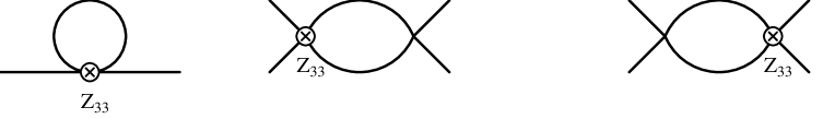
Figure 6: Contributions from evanescent operators to the four loop wave function, mass and coupling constant renormalization in the Gross Neveu model.

5 Massive NATM in $\overline{\mbox{MS}}$.

As far as we aware there been two calculations dealing with the two loop renormalization of the (massless) NATM, [14, 15]. The initial one performed in [14] used the auxiliary field formulation with a cutoff regularization which is not easy to extend to three loops. The latter one was detailed in the appendix of [15] and used dimensional regularization. Using the elementary argument of the previous section to ascertain the form of the highest possible operator which could emerge from the $4$-point function, it is elementary to observe that a $\Gamma_{(3)}\otimes\Gamma_{(3)}$ structure can emerge at one loop. This is evident in [15] and as a preliminary to discussing the three loop calculation we will first reproduce the analysis of [15] in the context of this article. There will be several minor differences in our strategy. For instance, we will be interested in the mass renormalization which was not discussed before. Second, the results presented in [15] were for a general colour group and did not appear to appeal to the simplification manifested by (3.19) for $SU(N_{\!c})$. Although this is not necessary to two loops the problem of obtaining independent combinations of the colour generators is not trivial in the general case, [35]. Indeed it is tedious even at the two loop level. At the outset we note that any calculation we have performed at two loops has been checked with the NATM analysis of [15] including the coefficients of the renormalization constants of the usual parameters and emerging evanescent operators, as well as the simple application of the projection formula to obtain the correct $\beta$-function of [14]. Although we will extend the massless calculation of [15] to three loops, our strategy will be to first consider the massive model. The primary reason for doing this is to exploit non-trivial checks on the full renormalization group functions which become available in the massive model. Having understood the procedure for the massive model we proceed to the massless case where such a check does not exist. This is due to the different roles $m$ plays in both models. In the latter case, since $m$ is a regularizing parameter it does not appear in the full renormalization group equation.

We begin by defining the renormalization constants we will compute, where the bare Lagrangian is

$$L^{\mbox{\footnotesize{natm}}}~{}=~{}i\bar{\psi}_{0}^{iI}\partial\!\!\!/\psi_{0}^{iI}~{}-~{}m_{0}\bar{\psi}_{0}^{iI}\psi_{0}^{iI}~{}+~{}\frac{g_{0}}{2}\left(\bar{\psi}_{0}^{iI}\gamma^{\mu}T^{a}_{IJ}\psi_{0}^{iJ}\right)^{2}~{}.$$ (5.1)

Setting

$$\psi_{0}~{}=~{}\psi Z_{\psi}^{\mbox{\small{$\frac{1}{2}$}}}~{}~{}~{},~{}~{}~{}m_{0}~{}=~{}mZ_{m}~{}~{}~{},~{}~{}~{}g_{0}~{}=~{}gZ_{11}\mu^{\epsilon}$$ (5.2)

and allowing for all possible evanescent operators up to three loops, we will take the renormalized Lagrangian as

$$L^{\mbox{\footnotesize{natm}}} = iZ_{\psi}\bar{\psi}^{iI}\partial\!\!\!/\psi^{iI}~{}-~{}mZ_{m}Z_{\psi}\bar{\psi}^{iI}\psi^{iI}$$ (5.3)

$$+~{}\frac{1}{2}g\mu^{\epsilon}Z^{2}_{\psi}\sum_{k=0}^{7}\left[Z_{k0}\left(\bar{\psi}^{iI}\Gamma_{(k)}\delta_{IJ}\psi^{iJ}\right)^{2}~{}+~{}Z_{k1}\left(\bar{\psi}^{iI}\Gamma_{(k)}T^{a}_{IJ}\psi^{iJ}\right)^{2}\right]$$

where as in (4.4) the $Z_{ki}$ are $O(g)$ except when $k$ $=$ $1$ and $i$ $=$ $1$. Although it would appear that there are thirteen terms up to level $\Gamma_{(7)}\otimes\Gamma_{(7)}$ in addition to the original vertex, it turns out that only the operators involving $\Gamma_{(2r+1)}$ for integer $r$, will occur, [21, 22], and the explicit calculation is consistent with this. To one loop the relevant diagrams are given in figures 1 and 3. The tadpole, defined as a zero momentum insertion on a line, only contributes to the mass renormalization, and gives the value

$$\frac{i(N_{\!c}^{2}-1)dmIg}{2N_{\!c}}~{}.$$ (5.4)

For the $4$-point function the sum of all channels gives

$$\frac{ig^{2}I}{4}\left[~{}-~{}\frac{(N_{\!c}^{2}-1)}{N_{\!c}^{2}}d(d-2){\cal O}_{00}~{}-~{}\frac{(N_{\!c}^{2}-4)}{N_{\!c}}d(d-2){\cal O}_{01}~{}-~{}N_{\!c}(3d-2){\cal O}_{11}\right.$$

$$\left.~{}~{}~{}~{}~{}~{}~{}~{}~{}+~{}N_{\!c}(d-2){\cal O}_{21}~{}+~{}\frac{(N_{\!c}^{2}-1)}{N_{\!c}^{2}}{\cal O}_{30}~{}+~{}\frac{(N_{\!c}^{2}-4)}{N_{\!c}}{\cal O}_{31}\right]~{}.$$ (5.5)

Here, we adopt the practice that the Green’s functions are written in terms of the (basis) operators ${\cal O}_{n0}$ $\equiv$ $\mbox{\small{$\frac{1}{2}$}}(\bar{\psi}\Gamma_{(n)}I\psi)^{2}$ and ${\cal O}_{n1}$ $\equiv$ $\mbox{\small{$\frac{1}{2}$}}(\bar{\psi}\Gamma_{(n)}T^{a}\psi)^{2}$ whose definition does not contain any coupling constant dependence. By doing this one can easily define the counterterm appropriately. At this stage we choose to renormalize using the $\overline{\mbox{MS}}$ scheme and absorb only those parts of (5.4) and (5.5) which are divergent. We have computed the coefficients of each operator as a function of $d$ in order to consider other schemes which we will do later. Therefore due to the presence of the factors of $(d-2)$ in (5.5) counterterms are only required for ${\cal O}_{11}$, ${\cal O}_{30}$ and ${\cal O}_{31}$ which have an odd number of $\gamma$-matrices. This is consistent with the earlier observation relating to chirality, [21, 22]. The generation of the latter operators affects the two loop renormalization. By counting the powers of the coupling constant in the Lagrangian, they need to be included with the two loop diagrams of figures 1 and 3, unlike in the Gross Neveu model where they contribute at four loops. Therefore, in the $2$-point function they are only relevant for the mass dimension through the tadpole of figure 6. For the $4$-point function of figure 6, the insertion now represents the presence of both ${\cal O}_{30}$ and ${\cal O}_{31}$.

At two loops in the $2$-point function there will be a contribution to the wave function renormalization from the sunset diagram. Of all the graphs we consider, this, aside from its related graphs at three loops, represented the most tedious to evaluate. It was not possible to write the relevant integral in a closed form. Instead we treated it by expanding the integral in powers of $p^{2}$ around $p^{2}$ $=$ $0$ and retained only those pieces which involve $p\!\!\!/$ or $m\delta_{\alpha}^{~{}\,\beta}$. These contributed respectively to the wave function and mass renormalization. In addition, we were careful to determine not only the pole parts but also the finite parts for the three loop calculation and in order to consider non-minimal renormalization schemes. We note that the wave function and other renormalization constants to three loops in the $\overline{\mbox{MS}}$ scheme have been collected together in appendix A.

Computing the $4$-point function now yields in addition to the operators ${\cal O}_{30}$ and ${\cal O}_{31}$, the new operators ${\cal O}_{10}$, ${\cal O}_{50}$ and ${\cal O}_{51}$. The latter two would be expected due to the simple $\gamma$-matrix counting, since the addition of a vertex introduces two $\gamma$-matrices from the new propagators and two $\gamma$-matrices from the extra vertex. For the one loop diagram of figure 6, the presence of $\Gamma_{(3)}$ at the operator insertion also yields a maximum of ten $\gamma$-matrices which have the extreme decomposition of $\Gamma_{(5)}\otimes\Gamma_{(5)}$. The main issue with the two loop $4$-point function is the observation that one cannot simply deduce the full $\beta$-function from the naïve renormalization constant $Z_{11}$. Ordinarily in the absence of the higher order operators the coefficients of the simple poles in $\epsilon$ are simply related to the coefficients of the $\beta$-function. In this case we would have

$$\tilde{\beta}(g)~{}\equiv~{}\tilde{\beta}_{11}(g)~{}=~{}\frac{N_{\!c}g^{2}}{2\pi}~{}+~{}(4N_{\!c}^{3}N_{\!f}-3N_{\!c}^{4}+12N_{\!c}^{2}-36)\frac{g^{3}}{16N_{\!c}^{2}\pi^{2}}~{}+~{}O(g^{4})~{}.$$ (5.6)

As was pointed out in [15], this clearly contradicts the calculation of [14] since on general considerations the $\beta$-function for a single coupling theory is scheme independent to two loops. The discrepancy between the two results is $3(N_{\!c}^{4}-4N_{\!c}^{2}+12)g^{3}/(16N_{\!c}^{2})$ which is related to the $\beta$-function of the operator ${\cal F}$ in the notation of [15] where

$${\cal F}~{}=~{}\mbox{\small{$\frac{1}{2}$}}\bar{\psi}T^{a}T^{b}T^{c}\gamma^{\mu}\psi\bar{\psi}{\cal T}^{abc}\gamma_{\mu}\psi$$ (5.7)

with

$${\cal T}^{abc}~{}=~{}2T^{a}T^{b}T^{c}~{}+~{}2T^{c}T^{b}T^{a}~{}+~{}T^{a}T^{c}T^{b}~{}+~{}T^{b}T^{a}T^{c}~{}+~{}T^{c}T^{a}T^{b}~{}+~{}T^{b}T^{c}T^{a}$$ (5.8)

and

$$\beta_{{\cal F}}(g)~{}=~{}-~{}\frac{3g^{3}}{16\pi^{2}}~{}.$$ (5.9)

For $SU(N_{\!c})$,

$$\left.{\cal F}\right|_{SU(N_{\!c})}~{}=~{}\frac{1}{2}\left[\frac{(N_{\!c}^{2}-1)(N_{\!c}^{2}-4)}{2N_{\!c}^{3}}(\bar{\psi}\gamma^{\mu}I\psi)^{2}~{}+~{}\frac{(N_{\!c}^{4}-4N_{\!c}^{2}+12)}{2N_{\!c}^{2}}(\bar{\psi}\gamma^{\mu}T^{a}\psi)^{2}\right]$$ (5.10)

so that the second term is related to the spurious contribution to the naïve $\beta$-function. Clearly one needs a systematic method of accounting for the existence of such contributions and removing them from the true $\beta$-function and the other renormalization group functions.

This is provided for in the projection technique, [28], discussed in [15] but which we recast in the basis of operators we have chosen. In addition to the naïve $\beta$-function, $\tilde{\beta}_{11}(g)$, the evanescent operators generated at one loop also have $\beta$-functions, deduced in the usual fashion. To $O(g^{3})$ these are

$$\tilde{\beta}_{30}(g) = -~{}\frac{(N_{\!c}^{2}-1)g^{2}}{8N_{\!c}^{2}\pi}$$ (5.11)

$$\tilde{\beta}_{31}(g) = -~{}\frac{(N_{\!c}^{2}-4)g^{2}}{8N_{\!c}\pi}~{}.$$ (5.12)

Although the general formalism was presented in section 2 its practical application requires explanation, especially as it will be applied to the three loop renormalization. As it stands, equation (2.24) represents the decomposition of the evanescent operator into a linear combination of the relevant original operators. The coefficients of this combination are perturbative functions of the physical coupling and the formula is only meaningful in the context of a Green’s function. Substituting, say, the operator ${\cal N}[{\cal O}_{31}]$ into a $2$-point function one evaluates the Green’s function in two dimensions after any infinities have been removed. Then one inserts the right side of (2.24) into the same Green’s function with the as yet undetermined projection functions and evaluates the Feynman diagrams to the same order before renormalizing and setting $d$ $=$ $2$. However, it is easy to deduce that at leading order only the operator ${\cal N}[{\cal O}_{11}]$ will contribute for insertions in a $4$-point function. Likewise ${\cal N}[i\bar{\psi}\partial\!\!\!/\psi]$ and ${\cal N}[\bar{\psi}\psi]$ will be relevant for the leading order in the $2$-point function. This therefore provides the starting point of the perturbative iteration which determines $\rho^{(ki)}(g)$, $\rho^{(ki)}_{m}(g)$ and $C^{(ki)}(g)$, $i$ $=$ $0$, $1$. Indeed at leading order it is only the tree level insertions of the relevant operators on the right side of (2.24) which will contribute. The insertion of these in the respective Green’s function each evaluate to unity.

Hence one needs only to compute the graphs of figure 6 for each operator ${\cal O}_{30}$ and ${\cal O}_{31}$. For the $2$-point function each is finite to this order and give

$$\langle\psi{\cal N}[{\cal O}_{30}]\bar{\psi}\rangle_{wf} = O(g)$$

$$\langle\psi{\cal N}[{\cal O}_{31}]\bar{\psi}\rangle_{wf} = O(g)$$ (5.13)

and

$$\langle\psi{\cal N}[{\cal O}_{30}]\bar{\psi}\rangle_{m} = \frac{1}{\pi}~{}+~{}O(g)$$

$$\langle\psi{\cal N}[{\cal O}_{31}]\bar{\psi}\rangle_{m} = \frac{(N_{\!c}^{2}-1)}{2N_{\!c}\pi}~{}+~{}O(g)~{}.$$ (5.14)

We have separated the contributions to the full $2$-point function with the operator insertion into the piece involving $p\!\!\!/$ and the mass and denoted these respectively by the subscripts $wf$ and $m$. However, for the $4$-point function care must be taken to renormalize the operator insertion before setting $d$ $=$ $2$. As this will become important later we record the insertion of each operator in the $4$-point function to the $O(\epsilon)$ term

$$\langle\psi\bar{\psi}{\cal N}[{\cal O}_{30}]\psi\bar{\psi}\rangle = \frac{ig}{\pi}\left[\frac{1}{\epsilon}\left({\cal O}_{51}~{}-~{}\frac{4(N_{\!c}^{2}-1)}{N_{\!c}}{\cal O}_{30}\right)~{}-~{}6{\cal O}_{11}\right.$$ (5.15)

$$\left.~{}~{}~{}-~{}\frac{(N_{\!c}^{2}-1)}{N_{\!c}}\left(1+2\ln\left(\frac{\tilde{\mu}^{2}}{m^{2}}\right)\right){\cal O}_{30}~{}+~{}\frac{1}{2}\ln\left(\frac{\tilde{\mu}^{2}}{m^{2}}\right){\cal O}_{51}\right.$$

$$\left.~{}~{}~{}+~{}3\epsilon\left(2-\ln\left(\frac{\tilde{\mu}^{2}}{m^{2}}\right)\right){\cal O}_{11}~{}+~{}O(\epsilon;{\cal O}_{k0},{\cal O}_{k1})\right]~{}+~{}O(g^{2})$$

and

$$\langle\psi\bar{\psi}{\cal N}[{\cal O}_{31}]\psi\bar{\psi}\rangle = \frac{ig}{\pi}\left[\frac{1}{\epsilon}\left(\frac{(N_{\!c}^{2}+4)}{N_{\!c}}{\cal O}_{31}~{}+~{}\frac{(N_{\!c}^{2}-1)}{4N_{\!c}^{2}}{\cal O}_{50}~{}+~{}\frac{(N_{\!c}^{2}-4)}{4N_{\!c}}{\cal O}_{51}\right)\right.$$

$$\left.~{}~{}~{}-~{}\frac{3(N_{\!c}^{2}-1)}{2N_{\!c}^{2}}{\cal O}_{10}~{}-~{}\frac{3(N_{\!c}^{2}-4)}{2N_{\!c}}{\cal O}_{11}~{}-~{}\frac{N_{\!c}}{4}{\cal O}_{41}\right.$$

$$\left.~{}~{}~{}+~{}\left(7N_{\!c}^{2}+4+2(N_{\!c}^{2}+4)\ln\left(\frac{\tilde{\mu}^{2}}{m^{2}}\right)\right)\frac{{{\cal O}_{31}}}{4N_{\!c}}\right.$$

$$\left.~{}~{}~{}+~{}\frac{(N_{\!c}^{2}-1)}{8N_{\!c}^{2}}\ln\left(\frac{\tilde{\mu}^{2}}{m^{2}}\right){\cal O}_{50}~{}+~{}\frac{(N_{\!c}^{2}-4)}{8N_{\!c}}\ln\left(\frac{\tilde{\mu}^{2}}{m^{2}}\right){\cal O}_{51}\right.$$

$$\left.~{}~{}~{}+~{}\frac{3(N_{\!c}^{2}-4)\epsilon}{4N_{\!c}}\left(2-\ln\left(\frac{\tilde{\mu}^{2}}{m^{2}}\right)\right){\cal O}_{11}~{}+~{}O(\epsilon;{\cal O}_{k0},{\cal O}_{k1})\right]~{}+~{}O(g^{2})$$

where we have introduced the new mass scale $\tilde{\mu}^{2}$ $=$ $4\pi e^{-\gamma}\mu^{2}$, with $\gamma$ denoting Euler’s constant, to ensure that we are in the $\overline{\mbox{MS}}$ scheme as opposed to the MS scheme. The renormalization constants to remove the simple poles on the right side are provided by the fact that the expressions effectively represent the first stage in the renormalization of a composite operator in the normal fashion. There is a caveat here in that there is mixing into other basis operators. However, one can introduce a counterterm which is a linear combination of the basis elements. The upshot of this for higher order calculations is that when the renormalized operator is inserted one must also include the counterterms from the mixing operators. For instance, for ${\cal O}_{30}$ this will mean at the next order that a tadpole graph with insertions $4(N_{\!c}^{2}-1){\cal O}_{31}/(N_{\!c}\epsilon)$ and $-$ ${\cal O}_{51}/\epsilon$ have to be included. After this renormalization which we also take to be $\overline{\mbox{MS}}$ here, the contribution to the Green’s function after setting the evanescent couplings to zero and $d$ $=$ $2$ are, to this order,

$$\left.\langle\psi\bar{\psi}{\cal N}[{\cal O}_{30}]\psi\bar{\psi}\rangle\right|_{{\cal O}_{11}} = -~{}\frac{6ig}{\pi}~{}+~{}O(g^{2})$$

$$\left.\langle\psi\bar{\psi}{\cal N}[{\cal O}_{31}]\psi\bar{\psi}\rangle\right|_{{\cal O}_{11}} = -~{}\frac{3i(N_{\!c}^{2}-4)g}{2N_{\!c}\pi}~{}+~{}O(g^{2})~{}.$$ (5.17)

So it is trivial to deduce,

$$\rho^{(30)}(g) = O(g)~{}~{}~{},~{}~{}~{}\rho^{(31)}(g)~{}=~{}O(g)$$ (5.18)

$$\rho^{(30)}_{m}(g) = -~{}\frac{1}{\pi}~{}+~{}O(g)~{}~{}~{},~{}~{}~{}\rho^{(31)}_{m}(g)~{}=~{}-~{}\frac{(N_{\!c}^{2}-1)}{2N_{\!c}\pi}~{}+~{}O(g)$$ (5.19)

$$C^{(30)}(g) = -~{}\frac{6g}{\pi}~{}+~{}O(g^{2})~{}~{}~{},~{}~{}~{}C^{(31)}(g)~{}=~{}-~{}\frac{3(N_{\!c}^{2}-4)g}{2N_{\!c}\pi}~{}+~{}O(g^{2})~{}.$$ (5.20)

Hence, substituting these functions into the general formulæ in (2.27) the actual renormalization group functions to two loops are

$$\beta(g) = \frac{N_{\!c}g^{2}}{2\pi}~{}+~{}\frac{N_{\!f}N_{\!c}g^{3}}{4\pi^{2}}$$

$$\gamma(g) = -~{}\frac{(N_{\!c}^{2}-1)N_{\!f}g^{2}}{8N_{\!c}\pi^{2}}$$

$$\gamma_{m}(g) = \frac{(N_{\!c}^{2}-1)g}{2N_{\!c}\pi}~{}+~{}(N_{\!c}^{2}-1)(4N_{\!f}-N_{\!c})\frac{g^{2}}{16N_{\!c}\pi^{2}}$$ (5.21)

where the result of [14] is recovered. Moreover, we also have the $\overline{\mbox{MS}}$ mass anomalous dimension which has not been computed in this model before.

We now turn to the details of the three loop calculations which builds on the above. We do not comment on the mundane task of the computation of the diagrams of figures 2, 4 and 5 since their evaluation very much parallels any usual perturbative calculation in other models. Instead we focus on the role of the evanescent operators. As the two loop calculation generated new operators their contributions must also be included. However, they will only enter through the topologies of figure 6 where the circle with a cross will now represent successively ${\cal O}_{10}$, ${\cal O}_{50}$ and ${\cal O}_{51}$. Additionally the counterterms generated for ${\cal O}_{30}$ and ${\cal O}_{31}$ are also included in those topologies as well as the original operator in the graphs of figures 7, 8 and 9. In figure 8 the insertion stands for the four possible combinations of ${\cal O}_{30}$ and ${\cal O}_{31}$. In these and the graphs

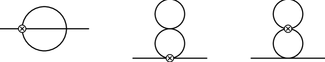
Figure 7: Graphs contributing to the NATM $2$-point function from evanescent operators ${\cal O}_{3i}$ in the two loop topology.

with the original vertex we note that we have also included the usual wave function, mass and vertex counterterms. Having detailed the extra evanescent operator contributions which have to be included it perhaps can be appreciated that such a calculation can only properly be attacked using symbolic and algebraic manipulation programmes.

Figure 8: Graphs contributing to the NATM $4$-point function from evanescent operators ${\cal O}_{3i}$ in the one loop topology.

It is not possible to include the values of each diagram in terms of the full operator basis. To illustrate the complexity of the result for one diagram, though, we record the structure of the three loop chain of figure 4. We found that for arbitrary $d$ it is

$$ig^{4}I^{3}\left[~{}-~{}d(3d^{3}+31d^{2}-70d+40)(d-2)(N_{\!c}^{4}-2N_{\!c}^{2}+6)(N_{\!c}^{2}-1)\frac{{\cal O}_{00}}{128N_{\!c}^{4}}\right.$$

$$\left.~{}~{}~{}~{}~{}~{}~{}~{}~{}-~{}d(3d^{3}+31d^{2}-70d+40)(d-2)(N_{\!c}^{4}+2)(N_{\!c}^{2}-4)\frac{{\cal O}_{01}}{64N_{\!c}^{3}}\right.$$

$$\left.~{}~{}~{}~{}~{}~{}~{}~{}~{}-~{}(45d^{4}-165d^{3}+168d^{2}+36d-80)(N_{\!c}^{2}-4)(N_{\!c}^{2}-1)\frac{{\cal O}_{10}}{128N_{\!c}^{2}}\right.$$

$$\left.~{}~{}~{}~{}~{}~{}~{}~{}~{}-~{}(45d^{4}-165d^{3}+168d^{2}+36d-80)(N_{\!c}^{4}-4N_{\!c}^{2}+10)\frac{{\cal O}_{11}}{64N_{\!c}}\right.$$

$$\left.~{}~{}~{}~{}~{}~{}~{}~{}~{}+~{}(6d^{3}+103d^{2}-394d+376)(d-2)(N_{\!c}^{2}-4)(N_{\!c}^{2}-1)\frac{{\cal O}_{20}}{128N_{\!c}^{2}}\right.$$

$$\left.~{}~{}~{}~{}~{}~{}~{}~{}~{}+~{}(6d^{3}+103d^{2}-394d+376)(d-2)(N_{\!c}^{4}-4N_{\!c}^{2}+10)\frac{{\cal O}_{21}}{64N_{\!c}}\right.$$

$$\left.~{}~{}~{}~{}~{}~{}~{}~{}~{}+~{}(30d^{3}-75d^{2}-130d+376)(N_{\!c}^{4}-2N_{\!c}^{2}+6)(N_{\!c}^{2}-1)\frac{{\cal O}_{30}}{128N_{\!c}^{4}}\right.$$

$$\left.~{}~{}~{}~{}~{}~{}~{}~{}~{}+~{}(30d^{3}-75d^{2}-130d+376)(N_{\!c}^{4}+2)(N_{\!c}^{2}-4)\frac{{\cal O}_{31}}{64N_{\!c}^{3}}\right.$$

$$\left.~{}~{}~{}~{}~{}~{}~{}~{}~{}-~{}(d^{2}+41d-116)(d-2)(N_{\!c}^{4}-2N_{\!c}^{2}+6)(N_{\!c}^{2}-1)\frac{{\cal O}_{40}}{128N_{\!c}^{4}}\right.$$

$$\left.~{}~{}~{}~{}~{}~{}~{}~{}~{}-~{}(d^{2}+41d-116)(d-2)(N_{\!c}^{4}+2)(N_{\!c}^{2}-4)\frac{{\cal O}_{41}}{64N_{\!c}^{3}}\right.$$

$$\left.~{}~{}~{}~{}~{}~{}~{}~{}~{}-~{}(3d^{2}+9d-58)\left((N_{\!c}^{2}-4)(N_{\!c}^{2}-1)\frac{{\cal O}_{50}}{128N_{\!c}^{2}}~{}+~{}(N_{\!c}^{4}-4N_{\!c}^{2}+10)\frac{{\cal O}_{51}}{64N_{\!c}}\right)\right.$$

$$\left.~{}~{}~{}~{}~{}~{}~{}~{}~{}+~{}3(d-2)\left((N_{\!c}^{2}-4)(N_{\!c}^{2}-1)\frac{{\cal O}_{60}}{128N_{\!c}^{2}}~{}+~{}(N_{\!c}^{4}-4N_{\!c}^{2}+10)\frac{{\cal O}_{61}}{64N_{\!c}}\right)\right.$$

$$\left.~{}~{}~{}~{}~{}~{}~{}~{}~{}+~{}(N_{\!c}^{4}-2N_{\!c}^{2}+6)(N_{\!c}^{2}-1)\frac{{\cal O}_{70}}{128N_{\!c}^{4}}~{}+~{}(N_{\!c}^{4}+2)(N_{\!c}^{2}-4)\frac{{\cal O}_{71}}{64N_{\!c}^{3}}\right]~{}.$$ (5.22)

Unlike the one loop result for the graph of figure 3 the evanescent operators which are even in the number of $\gamma$-matrices have, in principle, been generated with simple and double poles in $\epsilon$. However, it turns out that when all contributions are summed and evaluated that they have finite coefficients. Thus divergences are only associated with those operators which have an odd number of $\gamma$-matrices as expected from general arguments, [21, 22]. Further, the new operators ${\cal O}_{70}$ and ${\cal O}_{71}$ appear which is consistent with our earlier argument. Renormalizing the contributions

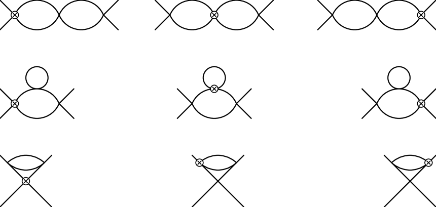
Figure 9: Graphs contributing to the NATM $4$-point function from evanescent operators ${\cal O}_{3i}$ in the two loop toplogies.

from the $2$ and $4$-point functions in $\overline{\mbox{MS}}$ determines the renormalization constants given in appendix A. The resulting naïve renormalization group functions for each operator can be deduced as

$$\tilde{\gamma}(g) = -~{}\frac{(N_{\!c}^{2}-1)N_{\!f}g^{2}}{8N_{\!c}\pi^{2}}~{}-~{}(N_{\!c}^{2}-1)(2N_{\!c}^{2}N_{\!f}^{2}+N_{\!c}^{3}N_{\!f}+2N_{\!c}^{2}+2)\frac{g^{3}}{32N_{\!c}^{3}\pi^{3}}$$ (5.23)

$$\tilde{\gamma}_{m}(g) = \frac{(N_{\!c}^{2}-1)g}{2N_{\!c}\pi}~{}+~{}(N_{\!c}^{2}-1)(2N_{\!c}N_{\!f}-N_{\!c}^{2}+1)\frac{g^{2}}{8N_{\!c}^{2}\pi^{2}}$$ (5.24)

$$+~{}(N_{\!c}^{2}-1)(16N_{\!f}^{2}N_{\!c}^{2}-20N_{\!f}N_{\!c}^{3}+16N_{\!c}N_{\!f}-3N_{\!c}^{4}+61N_{\!c}^{2}+62)\frac{g^{3}}{128N_{\!c}^{3}\pi^{3}}$$

$$\tilde{\beta}(g) = \frac{N_{\!c}g^{2}}{2\pi}~{}+~{}(4N_{\!c}^{3}N_{\!f}-3N_{\!c}^{4}+12N_{\!c}^{2}-36)\frac{g^{3}}{16N_{\!c}^{2}\pi^{2}}$$

$$+~{}(10N_{\!c}^{4}N_{\!f}^{2}-15N_{\!c}^{5}N_{\!f}+60N_{\!c}^{3}N_{\!f}-180N_{\!c}N_{\!f}+87N_{\!c}^{4}+13N_{\!c}^{2}-360)\frac{g^{4}}{64N_{\!c}^{3}\pi^{3}}$$

$$\tilde{\beta}_{30}(g) = -~{}\frac{(N_{\!c}^{2}-1)g^{2}}{8N_{\!c}^{2}\pi}~{}-~{}(N_{\!c}^{2}-1)(2N_{\!c}N_{\!f}+3N_{\!c}^{2}-2)\frac{g^{3}}{16N_{\!c}^{3}\pi^{2}}$$

$$-~{}(N_{\!c}^{2}-1)(96N_{\!c}^{2}N_{\!f}^{2}+240N_{\!c}^{3}N_{\!f}-144N_{\!c}N_{\!f}+773N_{\!c}^{4}-1004N_{\!c}^{2}+284)\frac{g^{4}}{1024N_{\!c}^{4}\pi^{3}}$$

$$\tilde{\beta}_{31}(g) = -~{}\frac{(N_{\!c}^{2}-4)g^{2}}{8N_{\!c}\pi}~{}-~{}(N_{\!c}^{2}-4)(N_{\!c}N_{\!f}-N_{\!c}^{2}-1)\frac{g^{3}}{8N_{\!c}^{2}\pi^{2}}$$ (5.27)

$$-~{}(N_{\!c}^{2}-4)(24N_{\!c}^{2}N_{\!f}^{2}-20N_{\!c}^{3}N_{\!f}-56N_{\!c}N_{\!f}+45N_{\!c}^{4}-54N_{\!c}^{2}+94)\frac{g^{4}}{256N_{\!c}^{4}\pi^{3}}$$

$$\tilde{\beta}_{50}(g) = -~{}\frac{(N_{\!c}^{2}-1)(N_{\!c}^{2}-4)g^{3}}{128N_{\!c}^{3}\pi^{2}}$$ (5.28)

$$\tilde{\beta}_{51}(g) = \frac{(N_{\!c}^{2}-3)g^{3}}{32N_{\!c}^{2}\pi^{2}}$$ (5.29)

$$\tilde{\beta}_{10}(g) = -~{}\frac{3(N_{\!c}^{2}-1)(N_{\!c}^{2}-4)g^{3}}{16N_{\!c}^{3}\pi^{2}}$$ (5.30)

where aside from ${\cal O}_{30}$ and ${\cal O}_{31}$ we have only retained those terms of the evanescent operator $\beta$-functions which are relevant for the true three loop renormalization group functions. To complete the calculation we need the subsequent terms in the projection functions.

For the $2$-point function this necessitates first of all computing the additional graphs to $\langle\psi{\cal N}[{\cal O}_{30}]\bar{\psi}\rangle$ and $\langle\psi{\cal N}[{\cal O}_{31}]\bar{\psi}\rangle$ as well as the new Green’s functions $\langle\psi{\cal N}[{\cal O}_{10}]\bar{\psi}\rangle$, $\langle\psi{\cal N}[{\cal O}_{50}]\bar{\psi}\rangle$ and $\langle\psi{\cal N}[{\cal O}_{51}]\bar{\psi}\rangle$. As the details of the calculation of the latter three are very much akin to those of the former two at the previous order we merely record the results

$$\rho^{(50)}_{m}(g) = \frac{2}{\pi}~{}+~{}O(g)~{}~{}~{},~{}~{}~{}\rho^{(51)}_{m}(g)~{}=~{}\frac{(N_{\!c}^{2}-1)}{N_{\!c}\pi}~{}+~{}O(g)$$ (5.31)

$$\rho^{(10)}_{m}(g) = \frac{1}{2\pi}\left[1-\ln\left(\frac{\tilde{\mu}^{2}}{m^{2}}\right)\right]~{}+~{}O(g)~{}.$$ (5.32)

For ${\cal O}_{3i}$ their composite operator insertion into the $2$-point function requires the computation of the graphs of figure 7 as well as the contribution from the graphs defined by the counterterms to the simple poles in (5.15) and (LABEL:o31) and their projection into the relevant operator. The upshot of including the additional graphs is that after $\overline{\mbox{MS}}$ renormalization we now have

$$\langle\psi{\cal N}[{\cal O}_{30}]\bar{\psi}\rangle_{wf} = -~{}\frac{(N_{\!c}^{2}-1)g}{2N_{\!c}\pi^{2}}~{}+~{}O(g^{2})$$

$$\langle\psi{\cal N}[{\cal O}_{31}]\bar{\psi}\rangle_{wf} = \frac{(N_{\!c}^{2}-1)g}{4N_{\!c}^{2}\pi^{2}}~{}+~{}O(g^{2})$$ (5.33)

and

$$\langle\psi{\cal N}[{\cal O}_{30}]\bar{\psi}\rangle_{m} = \frac{1}{\pi}~{}-~{}\frac{7(N_{\!c}^{2}-1)g}{4N_{\!c}\pi^{2}}\left[2+\ln\left(\frac{\tilde{\mu}^{2}}{m^{2}}\right)\right]~{}+~{}O(g^{2})$$ (5.34)

$$\langle\psi{\cal N}[{\cal O}_{31}]\bar{\psi}\rangle_{m} = \frac{(N_{\!c}^{2}-1)}{2N_{\!c}\pi}~{}+~{}\frac{(N_{\!c}^{2}-1)g}{N_{\!c}^{2}\pi^{2}}\left[\frac{13}{8}N_{\!c}^{2}+\frac{7}{4}-\left(\frac{N_{\!c}^{2}}{2}-\frac{7}{8}\right)\ln\left(\frac{\tilde{\mu}^{2}}{m^{2}}\right)\right]~{}+~{}O(g^{2})~{}.$$

To determine the extra terms of the projection formulæ the insertion of the right side of (2.24) in a $2$-point function must be included. Therefore, there is a contribution from the first graph of figure 10 after renormalization, from the ${\cal N}[{\cal O}_{11}]$ term of (2.24). This enters with the coefficients $C^{(30)}(g)$ and $C^{(31)}(g)$. Additionally the second graph, being $O(g)$, gives a potential contribution. However, it only contributes to the equation for $\rho^{(k)}_{m}(g)$. Finally,

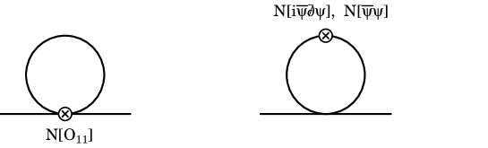
Figure 10: Graphs for the three loop projection formula in a $2$-point function for the NATM.

the finite part of the right side of (2.24) is

$$\frac{3(N_{\!c}^{2}-1)g}{2N_{\!c}\pi^{2}}\left[1-\ln\left(\frac{\tilde{\mu}^{2}}{m^{2}}\right)\right]~{}-~{}\left(\rho^{(30)}(g)+\rho^{(30)}_{m}(g)\right)\left[1+\frac{(N_{\!c}^{2}-1)g}{4N_{\!c}\pi}\left(3-\ln\left(\frac{\tilde{\mu}^{2}}{m^{2}}\right)\right)\right]~{}+~{}O(g^{2})$$ (5.35)

for ${\cal O}_{30}$ and

$$\frac{3(N_{\!c}^{2}-1)(N_{\!c}^{2}-4)g}{8N_{\!c}^{2}\pi^{2}}\left[1-\ln\left(\frac{\tilde{\mu}^{2}}{m^{2}}\right)\right]$$

$$-~{}\left(\rho^{(31)}(g)+\rho^{(31)}_{m}(g)\right)\left[1+\frac{(N_{\!c}^{2}-1)g}{4N_{\!c}\pi}\left(3-\ln\left(\frac{\tilde{\mu}^{2}}{m^{2}}\right)\right)\right]~{}+~{}O(g^{2})$$ (5.36)

for ${\cal O}_{31}$. Therefore, solving this perturbatively we find

$$\rho^{(30)}(g) = -~{}\frac{(N_{\!c}^{2}-1)g}{2N_{\!c}\pi^{2}}~{}+~{}O(g^{2})~{}~{}~{},~{}~{}~{}\rho^{(31)}(g)~{}=~{}\frac{(N_{\!c}^{2}-1)g}{4N_{\!c}^{2}\pi^{2}}~{}+~{}O(g^{2})$$ (5.37)

$$\rho^{(30)}_{m}(g) = -~{}\frac{1}{\pi}~{}+~{}\frac{25(N_{\!c}^{2}-1)g}{4N_{\!c}\pi^{2}}~{}+~{}O(g^{2})$$ (5.38)

$$\rho^{(31)}_{m}(g) = -~{}\frac{(N_{\!c}^{2}-1)}{2N_{\!c}\pi}~{}+~{}\frac{(N_{\!c}^{2}-1)}{N_{\!c}^{2}}\left[\frac{3}{4}\ln\left(\frac{\tilde{\mu}^{2}}{m^{2}}\right)-\frac{(7N_{\!c}^{2}+31)}{8}\right]\frac{g}{\pi^{2}}~{}+~{}O(g^{2})~{}.$$ (5.39)

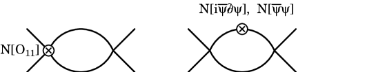
Figure 11: Graphs for the three loop projection formula in a $4$-point function for the NATM.

The procedure for the $4$-point function is similar. One also has extra graphs to consider involving the insertion of the relevant operators ${\cal N}[i\bar{\psi}\partial\!\!\!/\psi]$ and ${\cal N}[\bar{\psi}\psi]$ and these are given in figure 11 for the right side of (2.24). Including counterterm contributions both for the evanescent operator poles and the ${\cal O}_{11}$ vertex renormalization, the finite two dimensional Green’s functions now become

$$\left.\langle\psi\bar{\psi}{\cal N}[{\cal O}_{30}]\psi\bar{\psi}\rangle\right|_{{\cal O}_{11}} = -~{}\frac{6ig}{\pi}~{}+~{}i\left[3N_{\!c}\ln\left(\frac{\tilde{\mu}^{2}}{m^{2}}\right)~{}-~{}\frac{3N_{\!f}}{2}~{}+~{}\frac{65N_{\!c}}{4}~{}-~{}\frac{20}{N_{\!c}}\right]\frac{g^{2}}{\pi^{2}}~{}+~{}O(g^{3})$$

$$\left.\langle\psi\bar{\psi}{\cal N}[{\cal O}_{31}]\psi\bar{\psi}\rangle\right|_{{\cal O}_{11}} = -~{}\frac{3i(N_{\!c}^{2}-4)g}{2N_{\!c}\pi}~{}+~{}i\left[\frac{3(N_{\!c}-4)}{4}\ln\left(\frac{\tilde{\mu}^{2}}{m^{2}}\right)~{}-~{}\frac{3(N_{\!c}^{2}-4)N_{\!f}}{8N_{\!c}}\right.$$ (5.40)

$$\left.\quad\quad\quad\quad\quad\quad\quad\quad~{}~{}-~{}\frac{(13N_{\!c}^{4}-29N_{\!c}^{2}-82)}{4N_{\!c}^{2}}\right]\frac{g^{2}}{\pi^{2}}~{}+~{}O(g^{3})~{}.$$

Likewise, the sum of contributions to the right side give

$$[C^{(3i)}(g)+2g\rho^{(3i)}(g)]\left[1-\left(\frac{N_{\!c}}{2}\ln\left(\frac{\tilde{\mu}^{2}}{m^{2}}\right)-\frac{3N_{\!c}}{4}\right)\right]~{}+~{}\frac{N_{\!c}\rho^{(3i)}_{m}(g)g^{2}}{2\pi}~{}+~{}O(g^{3})$$ (5.41)

for $i$ $=$ $0$ and $1$. Hence, it is easy to deduce the projection functions to the order we require are

$$C^{(30)}(g) = -~{}\frac{6g}{\pi}~{}-~{}\left[\frac{3N_{\!f}}{2}-\frac{89N_{\!c}}{4}+\frac{21}{N_{\!c}}\right]\frac{g^{2}}{\pi^{2}}~{}+~{}O(g^{3})$$

$$C^{(31)}(g) = -~{}\frac{3(N_{\!c}^{2}-4)g}{2N_{\!c}\pi}~{}-~{}\left[\frac{3(N_{\!c}^{2}-4)N_{\!f}}{8N_{\!c}}+\frac{(15N_{\!c}^{4}-16N_{\!c}^{2}-168)}{8N_{\!c}^{2}}\right]\frac{g^{2}}{\pi^{2}}~{}+~{}O(g^{3})~{}.$$

For the operators ${\cal O}_{10}$, ${\cal O}_{50}$ and ${\cal O}_{51}$ we note that the one loop graphs of figure 6 with the appropriate operator insertions take simpler forms. Respectively, we have

$$\langle\psi\bar{\psi}{\cal N}[{\cal O}_{10}]\psi\bar{\psi}\rangle~{}=~{}\frac{ig}{\pi}\left[\frac{1}{\epsilon}{\cal O}_{31}~{}+~{}2{\cal O}_{01}~{}+~{}\frac{1}{2}\ln\left(\frac{\tilde{\mu}^{2}}{m^{2}}\right){\cal O}_{31}~{}+~{}O(\epsilon)\right]~{}+~{}O(g^{2})$$ (5.43)

and

$$\langle\psi\bar{\psi}{\cal N}[{\cal O}_{50}]\psi\bar{\psi}\rangle = \frac{ig}{\pi}\left[\frac{1}{\epsilon}\left(40{\cal O}_{31}~{}-~{}\frac{16(N_{\!c}^{2}-1)}{N_{\!c}}{\cal O}_{50}~{}+~{}{\cal O}_{71}\right)\right.$$ (5.44)

$$\left.~{}~{}~{}~{}-~{}20\left(3+\ln\left(\frac{\tilde{\mu}^{2}}{m^{2}}\right)\right){\cal O}_{31}~{}-~{}10{\cal O}_{41}~{}+~{}\frac{1}{2}\ln\left(\frac{\tilde{\mu}^{2}}{m^{2}}\right){\cal O}_{71}\right.$$

$$\left.~{}~{}~{}~{}-~{}\frac{2(N_{\!c}^{2}-1)}{N_{\!c}}\left(1+4\ln\left(\frac{\tilde{\mu}^{2}}{m^{2}}\right)\right){\cal O}_{50}~{}+~{}O(\epsilon)\right]+~{}O(g^{2})~{}.$$

The expression for $\langle\psi\bar{\psi}{\cal N}[{\cal O}_{51}]\psi\bar{\psi}\rangle$ is similar to that for ${\cal O}_{50}$ but involves more operators. As it does not contain any relevant new features we do not record it. Since the operator ${\cal O}_{11}$ does not appear on the right side of (5.43) and (5.44), then after renormalization and removal of the evanescent operators the contribution to the left side of the respective projection formulæ is zero at this order. Therefore we have the simple results

$$C^{(10)}(g)~{}=~{}0~{}+~{}O(g^{2})~{}~{},~{}~{}C^{(50)}(g)~{}=~{}0~{}+~{}O(g^{2})~{}~{},~{}~{}C^{(51)}(g)~{}=~{}0~{}+~{}O(g^{2})$$ (5.45)

which imply that at this order $\tilde{\beta}_{10}(g)$, $\tilde{\beta}_{50}(g)$ and $\tilde{\beta}_{51}(g)$ are not in fact needed for the renormalization group functions. With the corrections to the other projection functions, it is now possible to deduce the true $\overline{\mbox{MS}}$ renormalization group functions for the NATM at three loops. For $SU(N_{\!c})$ we find

$$\beta(g) = \mu\frac{\partial g(\mu)}{\partial\mu}~{}=~{}\frac{N_{\!c}g^{2}}{2\pi}{}~{}+~{}\frac{N_{\!f}N_{\!c}g^{3}}{4\pi^{2}}$$ (5.46)

$$+~{}\left[\frac{5}{32}N_{\!c}N_{\!f}^{2}~{}+~{}\frac{3}{64}N_{\!c}^{3}~{}-~{}\frac{11}{64}N_{\!c}{}~{}+~{}\frac{39}{64}\frac{1}{N_{\!c}}\right]\frac{g^{4}}{\pi^{3}}~{}+~{}O(g^{5})$$

$$\gamma(g)~{}=~{}-~{}\frac{(N_{\!c}^{2}-1)N_{\!f}g^{2}}{8N_{\!c}\pi^{2}}~{}-~{}(N_{\!c}^{2}-1)\left(2N_{\!f}^{2}+N_{\!f}N_{\!c}+1\right)\frac{g^{3}}{32N_{\!c}\pi^{3}}$$ (5.47)

and

$$\gamma_{m}(g) = \frac{(N_{\!c}^{2}-1)g}{2N_{\!c}\pi}~{}+~{}(N_{\!c}^{2}-1)(4N_{\!f}-N_{\!c})\frac{g^{2}}{16N_{\!c}\pi^{2}}$$ (5.48)

$$+~{}(N_{\!c}^{2}-1)\left(16N_{\!f}^{2}N_{\!c}^{2}-12N_{\!f}N_{\!c}^{3}+3N_{\!c}^{4}+5N_{\!c}^{2}-26\right)\frac{g^{3}}{128N_{\!c}^{3}\pi^{3}}~{}.$$

It is worth noting that the term involving $\ln(\tilde{\mu}^{2}/m^{2})$ has cancelled in the sum for $\gamma_{m}(g)$.

Although we have detailed the projection technique of [15] for the massive NATM there is an alternative method of determining these renormalization group functions. In performing the calculation we were careful to compute the Feynman graphs as functions of $d$. Therefore, we can deduce the finite parts of the $2$ and $4$-point functions after renormalization. These must satisfy the full renormalization group equation (2.23) with the above functions. Therefore with

$$G^{(2)}(p,m,\tilde{\mu},g) = i(p\!\!\!/-m)~{}+~{}\frac{(N_{\!c}^{2}-1)mg}{4N_{\!c}\pi}\left[\ln\left(\frac{\tilde{\mu}^{2}}{m^{2}}\right)-1\right]$$

$$+~{}p\!\!\!/\left[2N_{\!c}N_{\!f}\ln\left(\frac{\tilde{\mu}^{2}}{m^{2}}\right)+1\right]\frac{(N_{\!c}^{2}-1)g^{2}}{32N_{\!c}^{2}\pi^{2}}$$

$$-~{}m\left[(2N_{\!c}^{2}-1)\ln^{2}\left(\frac{\tilde{\mu}^{2}}{m^{2}}\right)~{}-~{}(7N_{\!c}^{2}-6+2N_{\!c}N_{\!f})\ln\left(\frac{\tilde{\mu}^{2}}{m^{2}}\right)\right.$$

$$\left.~{}~{}~{}~{}~{}~{}~{}+~{}3N_{\!c}^{2}~{}-~{}3\frac{}{}\right]\frac{(N_{\!c}^{2}-1)g^{2}}{32N_{\!c}^{2}\pi^{2}}$$

$$+~{}p\!\!\!/\left[-~{}6N_{\!c}^{3}N_{\!f}\ln^{2}\left(\frac{\tilde{\mu}^{2}}{m^{2}}\right)~{}+~{}6(3N_{\!c}^{2}+2N_{\!c}N_{\!f}-2)N_{\!c}N_{\!f}\ln\left(\frac{\tilde{\mu}^{2}}{m^{2}}\right)\right.$$

$$\left.~{}~{}~{}~{}~{}~{}-~{}10N_{\!c}^{3}N_{\!f}+4N_{\!c}^{2}N_{\!f}^{2}-5N_{\!c}^{2}+24N_{\!c}N_{\!f}-14\frac{}{}\right]\frac{(N_{\!c}^{2}-1)g^{3}}{384N_{\!c}^{3}\pi^{3}}$$

$$+~{}m\left[2(2N_{\!c}^{2}-1)(3N_{\!c}^{2}-1)\ln^{3}\left(\frac{\tilde{\mu}^{2}}{m^{2}}\right)\right.$$

$$\left.~{}~{}~{}~{}~{}~{}~{}-~{}(84N_{\!c}^{4}+36N_{\!c}^{3}N_{\!f}-108N_{\!c}^{2}-12N_{\!c}N_{\!f}+30)\ln^{2}\left(\frac{\tilde{\mu}^{2}}{m^{2}}\right)\right.$$

$$\left.~{}~{}~{}~{}~{}~{}~{}+~{}(129N_{\!c}^{4}+60N_{\!c}^{3}N_{\!f}+24N_{\!c}^{2}N_{\!f}^{2}-207N_{\!c}^{2}-84N_{\!c}N_{\!f}+12)\ln\left(\frac{\tilde{\mu}^{2}}{m^{2}}\right)\right.$$

$$\left.~{}~{}~{}~{}~{}~{}~{}-~{}45N_{\!c}^{4}+20N_{\!c}^{3}N_{\!f}+16N_{\!c}^{2}N_{\!f}^{2}+42N_{\!c}^{2}-32N_{\!c}N_{\!f}-194\right]\frac{(N_{\!c}^{2}-1)g^{3}}{768N_{\!c}^{3}\pi^{3}}$$

and

$$\left.G^{(4)}(0,m,\tilde{\mu},g)\right|_{{\cal O}_{11}} = ig~{}+~{}\frac{N_{\!c}}{8}\left[3-2\ln\left(\frac{\tilde{\mu}^{2}}{m^{2}}\right)\right]\frac{g^{2}}{\pi}$$

$$+~{}\left[4N_{\!c}^{4}\ln^{2}\left(\frac{\tilde{\mu}^{2}}{m^{2}}\right)~{}-~{}(20N_{\!c}^{4}-8N_{\!c}^{2}+8N_{\!c}N_{\!f})\ln\left(\frac{\tilde{\mu}^{2}}{m^{2}}\right)\right.$$

$$\left.\frac{}{}~{}~{}~{}~{}+~{}15N_{\!c}^{4}~{}+~{}4N_{\!c}^{3}N_{\!f}+2N_{\!c}^{2}~{}-~{}34\right]\frac{g^{3}}{64N_{\!c}^{2}\pi^{2}}$$

$$-~{}\left[24N_{\!c}^{3}\ln^{3}\left(\frac{\tilde{\mu}^{2}}{m^{2}}\right)~{}-~{}12(19N_{\!c}^{3}+2N_{\!c}^{2}N_{\!f}-10N_{\!c}+8N_{\!f})\ln^{2}\left(\frac{\tilde{\mu}^{2}}{m^{2}}\right)\right.$$

$$\left.\frac{}{}~{}~{}~{}~{}+~{}\left(522N_{\!c}^{3}+192N_{\!c}^{2}N_{\!f}+24N_{\!c}N_{\!f}^{2}-456N_{\!c}+120N_{\!f}\right.\right.$$

$$\left.\left.~{}~{}~{}~{}~{}~{}~{}~{}~{}~{}~{}+\frac{96N_{\!f}^{2}}{N_{\!c}}-\frac{96N_{\!f}}{N_{\!c}^{2}}\right)\ln\left(\frac{\tilde{\mu}^{2}}{m^{2}}\right)-345N_{\!c}^{3}-20N_{\!c}^{2}N_{\!f}-32N_{\!c}N_{\!f}^{2}\right.$$

$$\left.~{}~{}~{}~{}~{}+~{}764N_{\!c}-288N_{\!f}+\frac{32N_{\!f}^{2}}{N_{\!c}}-\frac{1440}{N_{\!c}}+\frac{1056N_{\!f}}{N_{\!c}}+\frac{1424}{N_{\!c}^{3}}\right]\frac{g^{4}}{1536\pi^{3}}~{}.$$

it is easy to verify that (2.23) holds. If we did not possess the $\overline{\mbox{MS}}$ functions then we could have solved for them by ensuring that the renormalization group equation (2.23) holds. For the massless model, since the mass is not a parameter of the theory it means that this avenue is not possible for us. This will leave us only the projection method which we have now shown to be consistent. In writing (LABEL:4ptfin) we have retained only the contribution to the original relevant operator since after renormalization $d$ is set to $2$ and the evanescent operators removed. Finally, it is a simple task to rewrite the $\overline{\mbox{MS}}$ $\beta$-function back in terms of the colour group Casimirs as

$$\beta(\lambda) = -~{}\frac{C_{2}(G)\lambda^{2}}{2\pi}~{}+~{}\frac{T(R)N_{\!f}C_{2}(G)\lambda^{3}}{2\pi^{2}}$$

$$-~{}C_{2}(G)\left[\frac{5}{8}T^{2}(R)N_{\!f}^{2}~{}+~{}\frac{39}{16}C^{2}_{2}(R)~{}-~{}\frac{67}{32}C_{2}(R)C_{2}(G)~{}+~{}\frac{31}{64}C^{2}_{2}(G)\right]\frac{\lambda^{4}}{\pi^{3}}{}~{}+~{}O(\lambda^{5})$$

where we have also included the coupling $\lambda$ for comparison with the two loop results of [14].

6 Massless NATM in $\overline{\mbox{MS}}$.

As the massive model clearly does not provide us with a fully chirally symmetric theory, we have also computed the $\overline{\mbox{MS}}$ renormalization constants for the model when the propagator (2.17) is used. As the calculation runs very close to that of the previous section we concentrate on the new features. First, when one evaluates the contributing graphs to three loops with (2.17) the structure is simpler than the corresponding ones obtained by using (2.18). Indeed the first graph of figure 4 now becomes

$$ig^{4}I^{3}\left[\frac{}{}\right. - \left.(105d^{3}-420d^{2}+588d-272)(N_{\!c}^{2}-4)(N_{\!c}^{2}-1)\frac{{\cal O}_{10}}{128N_{\!c}^{2}}\right.$$ (6.1)

$$- \left.\left(4(2N_{\!c}^{2}N_{\!f}^{2}-4(d-2)N_{\!c}N_{\!f}+3(d-2)^{2})(d-2)^{3}N_{\!f}N_{\!c}~{}-~{}4(d-2)^{6}\right.\right.$$

$$~{}~{}+\left.\left.(105d^{3}-420d^{2}+588d-272)(N_{\!c}^{4}-4N_{\!c}^{2}+10)N_{\!c}^{2}\right)\frac{{\cal O}_{11}}{64N_{\!c}^{3}}\right.$$

$$+ \left.7(15d^{2}-70d+88)\!\left(\!(N_{\!c}^{4}-2N_{\!c}^{2}+6)(N_{\!c}^{2}-1)\frac{{\cal O}_{30}}{128N_{\!c}^{4}}~{}+~{}(N_{\!c}^{4}+2)(N_{\!c}^{2}-4)\frac{{\cal O}_{31}}{64N_{\!c}^{3}}\right)\right.$$

$$- \left.7(3d-10)\left((N_{\!c}^{2}-4)(N_{\!c}^{2}-1)\frac{{\cal O}_{50}}{128N_{\!c}^{2}}~{}+~{}(N_{\!c}^{4}-4N_{\!c}^{2}+10)\frac{{\cal O}_{51}}{64N_{\!c}}\right)\right.$$

$$+ \left.(N_{\!c}^{4}-2N_{\!c}^{2}+6)(N_{\!c}^{2}-1)\frac{{\cal O}_{70}}{128N_{\!c}^{4}}~{}+~{}(N_{\!c}^{4}+2)(N_{\!c}^{2}-4)\frac{{\cal O}_{71}}{64N_{\!c}^{3}}{}~{}~{}\right]~{}.$$

Comparing this with the expression for the same graph in the massive case we observe its decomposition into the operator basis involves only those operators with $\Gamma_{(2r+1)}$ for integer $r$. This is a result of the chiral symmetry which underlies the choice (2.17). Moreover, this is also a property of all the other graphs to this order, so that the potential need for renormalization constants $Z_{ni}$ for $n$ even and $i$ $=$ $0$ or $1$ is automatically excluded. Completing the $\overline{\mbox{MS}}$ renormalization of the model as previously it turns out that the renormalization constants are the same as for the massive model with exception of $Z_{m}$ which, of course, does not arise at the outset.

The computation of the full $\gamma(g)$ and $\beta(g)$ in the massless NATM now follows the use of the projection formula for the massive model whose practical use we have just demonstrated. Since $m$ is no longer a true parameter of the model, the projection formula (2.24) clearly takes the simpler form, [15],

$$\int d^{d}x\,{\cal N}[{\cal O}_{ki}]~{}=~{}\int d^{d}x\left.\left(\,\rho^{(ki)}(g){\cal N}[i\bar{\psi}\partial\!\!\!/\psi~{}+~{}2g{\cal O}_{11}]~{}+~{}C^{(ki)}(g){\cal N}[{\cal O}_{11}]\right)\right|_{g_{i}=0~{}d=2}~{}.$$ (6.2)

The absence of $\rho^{(ki)}_{m}(g)$ and, in principle, different values for the contributing terms to the Green’s function structure might mean that the true $\overline{\mbox{MS}}$ renormalization group functions will differ from those of the massive model. However, as argued in [15, 22] one would expect them to be equivalent. Therefore, it is important that this is checked explicitly. Though we need only do this for $\beta(g)$, as clearly $\gamma(g)$ will be unchanged.

For the $4$-point function there are again no contributions to the relevant operator in the Green’s function involving separate insertions of ${\cal O}_{10}$, ${\cal O}_{50}$ and ${\cal O}_{51}$ leaving us to concentrate on ${\cal O}_{30}$ and ${\cal O}_{31}$. For these, in order to illustrate the differences in the structure of the Green’s functions which are needed to deduce $C^{(30)}(g)$ and $C^{(31)}(g)$, we note that their one loop forms are

$$\langle\psi\bar{\psi}{\cal N}[{\cal O}_{30}]\psi\bar{\psi}\rangle = \frac{ig}{\pi}\left[\frac{1}{\epsilon}\left({\cal O}_{51}~{}-~{}\frac{(N_{\!c}^{2}-1)}{N_{\!c}}{\cal O}_{30}\right)~{}-~{}6{\cal O}_{11}\right.$$ (6.3)

$$\left.~{}~{}~{}~{}+~{}\epsilon\left(4-3\ln\left(\frac{\tilde{\mu}^{2}}{m^{2}}\right)\right){\cal O}_{11}~{}+~{}O(\epsilon;{\cal O}_{k0},{\cal O}_{k1})\right]~{}+~{}O(g^{2})$$

and

$$\langle\psi\bar{\psi}{\cal N}[{\cal O}_{31}]\psi\bar{\psi}\rangle = \frac{ig}{\pi}\left[\frac{1}{\epsilon}\left(\frac{(N_{\!c}^{2}+4)}{N_{\!c}}{\cal O}_{31}~{}+~{}\frac{(N_{\!c}^{2}-1)}{4N_{\!c}^{2}}{\cal O}_{50}~{}+~{}\frac{(N_{\!c}^{2}-4)}{4N_{\!c}}{\cal O}_{51}\right)\right.$$ (6.4)

$$\left.~{}~{}~{}~{}-~{}\frac{3(N_{\!c}^{2}-4)}{2N_{\!c}}{\cal O}_{11}~{}+~{}O(\epsilon;{\cal O}_{k0},{\cal O}_{k1})\right]~{}+~{}O(g^{2})$$

which can be compared with those of the massive NATM calculation. Further, including all relevant counterterms the restriction of these Green’s functions in $d$ $=$ $2$ at two loops gives

$$\left.\langle\psi\bar{\psi}{\cal N}[{\cal O}_{30}]\psi\bar{\psi}\rangle\right|_{{\cal O}_{11}} = -~{}\frac{6ig}{\pi}~{}+~{}i\left[3N_{\!c}\ln\left(\frac{\tilde{\mu}^{2}}{m^{2}}\right)~{}-~{}\frac{9N_{\!f}}{2}~{}+~{}\frac{67N_{\!c}}{4}~{}-~{}\frac{20}{N_{\!c}}\right]\frac{g^{2}}{\pi^{2}}~{}+~{}O(g^{3})$$

$$\left.\langle\psi\bar{\psi}{\cal N}[{\cal O}_{31}]\psi\bar{\psi}\rangle\right|_{{\cal O}_{11}} = -~{}\frac{3i(N_{\!c}^{2}-4)g}{2N_{\!c}\pi}~{}+~{}i\left[\frac{3(N_{\!c}-4)}{4}\ln\left(\frac{\tilde{\mu}^{2}}{m^{2}}\right)~{}-~{}\frac{9(N_{\!c}^{2}-4)N_{\!f}}{8N_{\!c}}\right.$$ (6.5)

$$\left.\quad\quad\quad\quad\quad\quad\quad\quad~{}~{}-~{}\frac{(6N_{\!c}^{4}-14N_{\!c}^{2}-41)}{2N_{\!c}^{2}}\right]\frac{g^{2}}{\pi^{2}}~{}+~{}O(g^{3})$$

which differ from those of the massive model. To deduce the final values of the projection functions, we record that now the right side of (6.2) is simpler than (2.24) due to the absence of $\rho^{(k)}_{m}(g)$. Explicitly, we have

$$[C^{(3i)}(g)+2g\rho^{(3i)}(g)]\left[1-\left(\frac{N_{\!c}}{2}\ln\left(\frac{\tilde{\mu}^{2}}{m^{2}}\right)-\frac{N_{\!f}}{2}-\frac{3N_{\!c}}{4}\right)\right]~{}+~{}O(g^{3})$$ (6.6)

for $i$ $=$ $0$ and $1$. However, when solving perturbatively for the projection functions it turns out that their values to this order are the same as before. Therefore the $\overline{\mbox{MS}}$ $\beta$-function is identical to that of the massive model as expected. The discrepancy between each set of formulæ rests in the hidden role of the mass term in various Green’s functions.

Figure 12: Graphs contributing to the renormalization of $[\bar{\psi}\psi]$ in the massless NATM.

Although it may seem that for the massless model that there is no renormalization group function for the mass, it is possible to compute the anomalous dimension of the composite operator whose coupling would correspond to a mass. Clearly this is $[\bar{\psi}\psi]$. As this operator will be renormalized, one can define an anomalous dimension $\gamma_{\bar{\psi}\psi}(g)$ from its renormalization constant $Z_{\bar{\psi}\psi}$ which can then be regarded as the mass dimension. Indeed the computation of the three loop quark mass dimension in $\overline{\mbox{MS}}$ in QCD was performed in the massless theory by renormalizing the $2$-point quark Green’s function with a $[\bar{\psi}\psi]$ insertion, [13]. We have computed the relevant diagrams to three loops for both the massless Gross Neveu model, in order to check our integration routines, and the massless NATM. These are illustrated in figure 12 where we have only shown those diagrams which are not trivially zero. Also, the cross indicates the location of the insertion of $[\bar{\psi}\psi]$. Therefore, if the insertion in the two loop tower of bubbles had not been on the top loop but the lower one, then the diagram is simply zero because in the massless model the one loop tadpole vanishes by Lorentz symmetry. Therefore if a topology has one tadpole then for a non-zero contribution its $[\bar{\psi}\psi]$ insertion must be in that tadpole. Although it may appear that we have to introduce a new set of integrals to carry out the calculation, we have exploited the fact that since we are only interested in the $[\bar{\psi}\psi]$ renormalization, the graphs need only be computed at zero external momentum. In this case it turns out that tensor integrals for each graph can be paired with a graph used in the evaluation of the $4$-point function. The topology of the related graph is deduced by regarding the insertion as the location of two external legs. So, for example, the last graph of figure 12 is paired with the penultimate graph of figure 4. Similarly the first graph of the bottom row of figure 12 is related to the fifth graph of figure 4. This observation ensures that we do not have to unnecessarily undertake extra calculation. It turns out that performing the $\overline{\mbox{MS}}$ renormalization of these graphs that $Z_{\bar{\psi}\psi}$ is identical to $Z_{m}$ of the massive model for both the Gross Neveu model and the NATM. To complete the evaluation of the associated true renormalization group function, we need to extend the projection formula of (6.2) to the case of bona fide operator insertions. In this case we take it to be

$$\int d^{d}x\,{\cal N}[{\cal O}_{k}] = \int d^{d}x\left.\left(\frac{}{}\,\rho^{(k)}(g){\cal N}[i\bar{\psi}\partial\!\!\!/\psi]~{}+~{}\left(C^{(k)}(g)+2g\rho^{(k)}(g)\right){\cal N}[{\cal O}_{11}]\right.\right.$$ (6.7)

$$\left.\left.~{}~{}~{}~{}~{}~{}~{}~{}~{}+~{}\left(\rho^{(k)}(g)+\rho^{(k)}_{\bar{\psi}\psi}(g)\right){\cal N}[1]\frac{}{}\right)\right|_{g_{i}=0~{}d=2}~{}.$$

Here the last term has the insertion of unity since we regard this operator equation as being inserted in a Green’s function of the structure $\langle\psi~{}.~{}[\bar{\psi}\psi]\bar{\psi}\rangle$ which includes the original operator

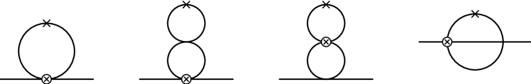
Figure 13: Graphs contributing to the massless NATM $2$-point function with $[\bar{\psi}\psi]$ insertion from the evanescent operators ${\cal O}_{3i}$.

insertion itself represented by the dot. Therefore, one needs to be careful in distinguishing which operator is which when considering the graphs contributing to the Green’s function. To this end we have illustrated the relevant non-zero contributions to the two loop Green’s function $\langle\psi{\cal N}[{\cal O}][\bar{\psi}\psi]\bar{\psi}\rangle$ in figure 13. As we have detailed similar calculations earlier, we record the values of the Green’s function for the operators ${\cal N}[{\cal O}_{30}]$ and ${\cal N}[{\cal O}_{31}]$ as those of other operators will only involve one loop graphs. We found,

$$\langle\psi{\cal N}[{\cal O}_{30}][\bar{\psi}\psi]\bar{\psi}\rangle = -\,\frac{1}{\pi}~{}-~{}\frac{(N_{\!c}^{2}-1)g}{N_{\!c}\pi^{2}}\left[\frac{9}{4}+\frac{7}{4}\ln\left(\frac{\tilde{\mu}^{2}}{m^{2}}\right)\right]~{}+~{}O(g^{2})$$

$$\langle\psi{\cal N}[{\cal O}_{31}][\bar{\psi}\psi]\bar{\psi}\rangle = -\,\frac{(N_{\!c}^{2}-1)}{2N_{\!c}\pi}~{}-~{}\frac{(N_{\!c}^{2}-1)g}{N_{\!c}^{2}\pi^{2}}\!\left[\frac{15N_{\!c}^{2}}{8}+\frac{9}{8}-\left(\frac{N_{\!c}^{2}}{2}-\frac{7}{8}\right)\ln\!\left(\frac{\tilde{\mu}^{2}}{m^{2}}\right)\right]\,+~{}O(g^{2})$$

where we note that the overall sign difference between these and the analogous results in the massive model is due to the fact that here we are inserting the operator $[\bar{\psi}\psi]$ and not the negative of this. Moreover,

$$\rho^{(50)}_{\bar{\psi}\psi}(g) = \frac{2}{\pi}~{}+~{}O(g)~{}~{}~{},~{}~{}~{}\rho^{(51)}_{\bar{\psi}\psi}(g)~{}=~{}\frac{(N_{\!c}^{2}-1)}{N_{\!c}\pi}~{}+~{}O(g)$$ (6.9)

$$\rho^{(10)}_{\bar{\psi}\psi}(g) = \frac{1}{2\pi}\left[2-\ln\left(\frac{\tilde{\mu}^{2}}{m^{2}}\right)\right]~{}+~{}O(g)$$ (6.10)

so that the numerical values of $\rho^{(10)}_{\bar{\psi}\psi}(g)$ and $\rho^{(10)}_{m}(g)$ differ. For the right side of the projection formula we have displayed the one loop corrections which need to be computed in figure 14. With their values the respective right sides of each projection formulæ are

$$-~{}\frac{3(N_{\!c}^{2}-1)g}{2N_{\!c}\pi^{2}}\!\left[2-\ln\left(\frac{\tilde{\mu}^{2}}{m^{2}}\right)\right]~{}-~{}\left(\rho^{(30)}(g)+\rho^{(30)}_{\bar{\psi}\psi}(g)\right)\!\!\left[1+\frac{(N_{\!c}^{2}-1)g}{4N_{\!c}\pi}\left(2-\ln\left(\frac{\tilde{\mu}^{2}}{m^{2}}\right)\!\right)\right]~{}+~{}O(g^{2})$$ (6.11)

for ${\cal O}_{30}$ and

$$-~{}\frac{3(N_{\!c}^{2}-1)(N_{\!c}^{2}-4)g}{8N_{\!c}^{2}\pi^{2}}\left[2-\ln\left(\frac{\tilde{\mu}^{2}}{m^{2}}\right)\right]$$

$$-~{}\left(\rho^{(31)}(g)+\rho^{(31)}_{\bar{\psi}\psi}(g)\right)\left[1+\frac{(N_{\!c}^{2}-1)g}{4N_{\!c}\pi}\left(2-\ln\left(\frac{\tilde{\mu}^{2}}{m^{2}}\right)\right)\right]~{}+~{}O(g^{2})$$ (6.12)

for ${\cal O}_{31}$, from which it is easy to deduce

$$\rho^{(30)}_{\bar{\psi}\psi}(g) = -~{}\frac{1}{\pi}~{}+~{}\frac{25(N_{\!c}^{2}-1)g}{4N_{\!c}\pi^{2}}~{}+~{}O(g^{2})$$

$$\rho^{(31)}_{\bar{\psi}\psi}(g) = -~{}\frac{(N_{\!c}^{2}-1)}{2N_{\!c}\pi}~{}+~{}\frac{(N_{\!c}^{2}-1)}{N_{\!c}^{2}}\left[\frac{3}{4}\ln\left(\frac{\tilde{\mu}^{2}}{m^{2}}\right)-\frac{(7N_{\!c}^{2}+37)}{8}\right]\frac{g}{\pi^{2}}~{}+~{}O(g^{2})~{}.$$ (6.13)

Therefore, the $\overline{\mbox{MS}}$ $\gamma_{\bar{\psi}\psi}(g)$ is identical to $\gamma_{m}(g)$ of the massive model.

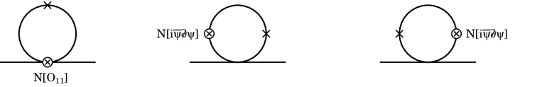
Figure 14: Graphs for the three loop projection formula in a $2$-point function with $[\bar{\psi}\psi]$ insertion for the massless NATM.

7 Symmetric schemes.

Although we have produced the renormalization group functions for both massive and massless versions of the NATM in $\overline{\mbox{MS}}$ there still remains the problem of reconciling the results with the equivalences with other models discussed earlier. The $\overline{\mbox{MS}}$ expressions do not represent results which are consistent with symmetries of the original model and the problem can effectively be traced to a hidden $\gamma^{5}$ issue, [15, 21, 22]. In other words, when one deals with models with continuous chiral symmetries in dimensional regularization this symmetry is not preserved in $\overline{\mbox{MS}}$. For example, in QCD one must treat $\gamma^{5}$ carefully in renormalizing quark bilinear currents involving $\gamma^{5}$. There the resolution is to use a renormalization scheme which does preserve the symmetry. This is achieved by first performing an $\overline{\mbox{MS}}$ calculation to the requisite order and then introduce an additional finite renormalization to ensure that in that case the Green’s functions obey the (quantum) Ward identities, including the axial anomaly, [39]. For the present calculation the general approach is the same. Though there will be several minor differences. One rests in the fact that the analogous finite renormalization is chosen so that one ensures the renormalization group functions in the first instance and not the Green’s functions are the same in the equivalences between the various models. Further, in the present context, similar finite renormalization schemes have been established for the three loop anomalous dimension ensuring agreement of the equivalences between the ABTM and the Gross Neveu model for $N_{\!f}$ $=$ $1$, [22]. In essence that scheme was specified by removing in addition to the simple poles, the (numerical) finite part of the Green’s function into the renormalization constant, [22]. We stress that terms involving $\ln(\tilde{\mu}^{2}/m^{2})$ were not removed so that one is still within the context of mass independent renormalization schemes. In [15, 22] this was referred to as the symmetric scheme. To appreciate the effect such a choice of scheme can have on the renormalization group functions we have determined them for the Gross Neveu model. To three loops for the two dimensional massive model, we found that

$$\beta(g) = -~{}\frac{(N_{\!f}-1)g^{2}}{\pi}~{}+~{}\frac{(N_{\!f}-1)g^{3}}{2\pi^{2}}~{}-~{}\frac{(6N_{\!f}-1)(N_{\!f}-1)g^{4}}{8\pi^{3}}~{}+~{}O(g^{5})$$ (7.1)

$$\gamma(g) = -~{}\frac{(2N_{\!f}-1)g^{2}}{8\pi^{2}}~{}-~{}\frac{(2N_{\!f}-1)(2N_{\!f}-3)g^{3}}{8\pi^{3}}~{}+~{}O(g^{4})$$ (7.2)

$$\gamma_{m}(g) = -~{}\frac{(2N_{\!f}-1)g}{2\pi}~{}-~{}\frac{(2N_{\!f}-1)(4N_{\!f}-7)g^{2}}{8\pi^{2}}$$ (7.3)

$$-~{}\frac{(8N_{\!f}^{2}-42N_{\!f}+37)(2N_{\!f}-1)g^{3}}{16\pi^{3}}~{}+~{}O(g^{4})~{}.$$

Clearly, one now has a cubic polynomial in $N_{\!f}$ at three loops in $\gamma_{m}(g)$ in contrast to the quadratic that appears in the $\overline{\mbox{MS}}$ scheme. We can readily produce this result since we have been careful in the contruction of the integration routines to keep all the $d$-dependence. The aim now is to extend our calculation to determine the scheme or schemes which preserve the known equivalences of the NATM. We follow the approach of [15, 22] and reconcile the results with the $\overline{\mbox{MS}}$ forms of the $O(2N_{\!f})$ Gross Neveu model which possesses a discrete $\gamma^{5}$ chiral symmetry. Though we stress that one could choose another scheme as reference. Further, since the choice of scheme is very much arbitrary we will take a general approach and introduce a parametrization. This will involve a set of variables which will be constrained by the equivalences. To illustrate this we will consider the massless model only and define the finite terms of the wave function renormalization to be

$$\frac{(N_{\!c}^{2}-1)g^{2}}{N_{\!c}\pi^{2}}\left(w_{21}N_{\!f}+w_{22}N_{\!c}+\frac{w_{23}}{N_{\!c}}\right)~{}.$$ (7.4)

Likewise for the coupling constant renormalization constant, $Z_{11}Z^{2}_{\psi}$, we take the finite part to be

$$\left(b_{11}N_{\!f}+b_{12}N_{\!c}+\frac{b_{13}}{N_{\!c}}\right)\frac{g}{\pi}~{}+~{}\left(b_{21}N_{\!f}^{2}+b_{22}N_{\!f}N_{\!c}+\frac{b_{23}N_{\!f}}{N_{\!c}}+b_{24}N_{\!c}^{2}+b_{25}+\frac{b_{26}}{N_{\!c}^{2}}\right)\frac{g^{2}}{\pi^{2}}~{}.$$ (7.5)

An $O(g^{3})$ term will affect the four loop form of the renormalization group functions. The form of the additional terms has been chosen to be consistent with the colour Casimir structure that is allowed. Therefore, the term of (7.4) is proportional to $C_{2}(R)$. Of course, these additional terms will affect the form of poles in $\epsilon$ of the renormalization constants which we have not recorded.

In the context of the usual multiplicatively renormalizable theories the treatment of a scheme change is straightforward and well documented. (See, for example, [40, 21, 22].) Once one has one scheme, the renormalization group functions in another are determined by the relations

$$\bar{\beta}(\bar{g}) = \beta(g)\frac{\partial~{}}{\partial g}\bar{g}(g)$$

$$\bar{\gamma}(\bar{g}) = \gamma(g)~{}-~{}2\beta(g)\frac{\partial~{}}{\partial g}\ln\xi(g)$$ (7.6)

where

$$\bar{G}^{(n)}(p,\mu,\bar{g})~{}=~{}\xi^{n}G^{(n)}(p,\mu,g)$$ (7.7)

and the bar denotes the corresponding quantity in another scheme. In general the relation between the couplings in both schemes is determined by comparing the renormalized $4$-point Green’s functions using (7.7) after the function $\xi(g)$ is deduced at the appropriate order in the $2$-point function. For the non-multiplicatively renormalizable NATM the situation is the same, though of course one has to first compute the new Green’s functions in the scheme involving (7.4) and (7.5). To understand fully the proper procedure for this we have first performed the renormalization in the massive model and then determined the renormalization group functions by finding the function $\xi(g)$ before applying the formulæ, (7.6). These could then be checked against the renormalization group functions deduced by ensuring that the renormalization group equation itself was satisfied. Repeating this first method for the massless model we have the general functions

$$\xi(g) = \left[1~{}+~{}\frac{(N_{\!c}^{2}-1)g^{2}}{N_{\!c}\pi^{2}}\left(w_{21}N_{\!f}~{}+~{}w_{22}N_{\!c}~{}+~{}\frac{w_{23}}{N_{\!c}}\right)\right]$$

$$\bar{g}(g) = g\left[1~{}-~{}\left(b_{11}N_{\!f}~{}+~{}b_{12}N_{\!c}~{}+~{}\frac{b_{13}}{N_{\!c}}\right)\frac{g}{\pi}~{}+~{}\left(2N_{\!c}^{2}N_{\!f}^{2}b_{11}^{2}~{}-~{}N_{\!c}^{2}N_{\!f}^{2}b_{21}\right.\right.$$ (7.8)

$$\left.\left.~{}~{}+~{}2N_{\!c}^{3}N_{\!f}w_{21}~{}+~{}4N_{\!c}^{3}N_{\!f}b_{11}b_{12}~{}-~{}N_{\!c}^{3}N_{\!f}b_{22}~{}-~{}2N_{\!c}N_{\!f}w_{21}~{}+~{}4N_{\!c}N_{\!f}b_{11}b_{13}\right.\right.$$

$$\left.\left.~{}~{}-~{}N_{\!c}N_{\!f}b_{23}~{}+~{}2N_{\!c}^{4}w_{22}~{}+~{}2N_{\!c}^{4}b_{12}^{2}~{}-~{}N_{\!c}^{4}b_{24}~{}-~{}2N_{\!c}^{2}w_{22}~{}+~{}2N_{\!c}^{2}w_{23}\right.\right.$$

$$\left.\left.~{}~{}+~{}4N_{\!c}^{2}b_{12}b_{13}~{}-~{}N_{\!c}^{2}b_{25}~{}-~{}2w_{23}~{}+~{}2b_{13}^{2}~{}-~{}b_{26}\right)\frac{g^{2}}{N_{\!c}^{2}\pi^{2}}\right]$$

which therefore provide us with the general scheme results

$$\bar{\gamma}(\bar{g}) = -~{}\frac{(N_{\!c}^{2}-1)N_{\!f}}{8N_{\!c}}\frac{\bar{g}^{2}}{\pi^{2}}~{}-~{}\frac{(N_{\!c}^{2}-1)}{32N_{\!c}^{2}}\left[8N_{\!c}N_{\!f}^{2}b_{11}~{}+~{}2N_{\!c}N_{\!f}^{2}~{}+~{}32N_{\!c}^{2}N_{\!f}w_{21}~{}+~{}8N_{\!c}^{2}N_{\!f}b_{12}\right.$$ (7.9)

$$\left.+~{}N_{\!c}^{2}N_{\!f}~{}+~{}8N_{\!f}b_{13}~{}+~{}32N_{\!c}^{3}w_{22}~{}+~{}32N_{\!c}w_{23}~{}+~{}N_{\!c}\right]\frac{\bar{g}^{3}}{\pi^{3}}~{}+~{}O(\bar{g}^{4})$$

and

$$\bar{\beta}(\bar{g}) = \frac{N_{\!c}\bar{g}^{2}}{2\pi}~{}+~{}\frac{N_{\!f}N_{\!c}\bar{g}^{3}}{4\pi^{2}}~{}+~{}\left[32N_{\!c}^{2}N_{\!f}^{2}b_{11}^{2}~{}+~{}16N_{\!c}^{2}N_{\!f}^{2}b_{11}~{}-~{}32N_{\!c}^{2}N_{\!f}^{2}b_{21}~{}+~{}10N_{\!c}^{2}N_{\!f}^{2}\right.$$ (7.10)

$$\left.+~{}64N_{\!c}^{3}N_{\!f}w_{21}~{}+~{}64N_{\!c}^{3}N_{\!f}b_{11}b_{12}~{}+~{}16N_{\!c}^{3}N_{\!f}b_{12}~{}-~{}32N_{\!c}^{3}N_{\!f}b_{22}~{}-~{}64N_{\!c}N_{\!f}w_{21}\right.$$

$$\left.+~{}64N_{\!c}N_{\!f}b_{11}b_{13}~{}+~{}16N_{\!c}N_{\!f}b_{13}~{}-~{}32N_{\!c}N_{\!f}b_{23}~{}+~{}64N_{\!c}^{4}w_{22}~{}+~{}32N_{\!c}^{4}b_{12}^{2}~{}-~{}32N_{\!c}^{4}b_{24}\right.$$

$$\left.+~{}3N_{\!c}^{4}~{}-~{}64N_{\!c}^{2}w_{22}~{}+~{}64N_{\!c}^{2}w_{23}~{}+~{}64N_{\!c}^{2}b_{12}b_{13}~{}-~{}32N_{\!c}^{2}b_{25}~{}-~{}11N_{\!c}^{2}~{}-~{}64w_{23}\right.$$

$$\left.+~{}32b_{13}^{2}~{}-~{}32b_{26}~{}+~{}39\right]\frac{\bar{g}^{4}}{64N_{\!c}\pi^{3}}~{}+~{}O(\bar{g}^{5})~{}.$$

The $\overline{\mbox{MS}}$ results are of course recovered by setting the various constants to zero.

The two equivalences we wish to preserve are those discussed in section 2. For the one involving the ABTM and the Gross Neveu model at $N_{\!f}$ $=$ $1$, we first need to convert the $SU(N_{\!c})$ dependence into the general colour group Casimirs and then apply (2.9). We find

$$\bar{\gamma}(\bar{g}) = -~{}\frac{N_{\!f}\bar{g}^{2}}{2\pi^{2}}~{}-~{}\left(N_{\!f}^{2}~{}+~{}4b_{11}N_{\!f}^{2}-4b_{13}N_{\!f}\right)\frac{\bar{g}^{3}}{2\pi^{3}}$$

$$\bar{\beta}(\bar{g}) = 0$$ (7.11)

giving

$$0 = 4b_{11}~{}-~{}4b_{13}~{}+~{}1$$

$$0 = 32w_{21}~{}-~{}32w_{23}~{}-~{}1$$

$$0 = 32b_{21}~{}-~{}32b_{23}~{}+~{}32b_{26}~{}-~{}31$$ (7.12)

where the latter two equations arise from choosing to remove the numerical part of the $2$-point and $4$-point functions respectively at three loops, similar to [22]. With the caveat we had previously on the form of $\gamma(g)$ for the second equivalence, we find that the constraints in this case are

$$0 = 16b_{12}~{}+~{}5b_{13}~{}+~{}80w_{21}~{}+~{}256w_{22}$$

$$0 = 8192b_{12}^{2}~{}+~{}5120b_{12}b_{13}~{}+~{}800b_{13}^{2}~{}-~{}2048b_{22}~{}-~{}640b_{23}~{}-~{}8192b_{24}~{}-~{}512b_{25}$$ (7.13)

$$+~{}480b_{26}~{}+~{}4800w_{21}~{}+~{}15360w_{22}~{}+~{}231~{}.$$

Clearly not all the general coefficients can be determined by these restrictions and the undetermined coefficients represent the remaining freedom in the choice of scheme that is possible. For instance, if we set

$$w_{21}~{}=~{}b_{12}~{}=~{}b_{13}~{}=~{}0~{}~{},~{}~{}b_{22}~{}=~{}\frac{15}{128}~{}~{},~{}~{}b_{23}~{}=~{}\frac{1}{4}~{}~{},~{}~{}b_{24}~{}=~{}\frac{3}{64}~{}~{},~{}~{}b_{26}~{}=~{}1$$ (7.14)

then the renormalization group functions will take the form

$$\bar{\gamma}(\bar{g}) = -~{}\frac{(N_{\!c}^{2}-1)N_{\!f}}{8N_{\!c}}\frac{\bar{g}^{2}}{\pi^{2}}~{}-~{}\frac{(N_{\!c}^{2}-1)N_{\!f}\bar{g}^{3}}{32}~{}+~{}O(\bar{g}^{4})$$

$$\bar{\beta}(\bar{g}) = \frac{N_{\!c}\bar{g}^{2}}{2\pi}~{}+~{}\frac{N_{\!f}N_{\!c}\bar{g}^{3}}{4\pi^{2}}$$

$$+~{}\left[16N_{\!c}^{2}N_{\!f}^{2}-60N_{\!c}^{3}N_{\!f}-128N_{\!c}N_{\!f}+24N_{\!c}^{4}-105N_{\!c}^{2}+144\right]\frac{\bar{g}^{4}}{1024N_{\!c}\pi^{3}}~{}+~{}O(\bar{g}^{5})~{}.$$

In the abelian limit, we obtain $\bar{\beta}(\bar{g})$ $=$ $0$ and $\bar{\gamma}(\bar{g})$ $=$ $-$ $N_{\!f}\bar{g}^{2}/(2\pi^{2})$ $+$ $O(\bar{g}^{4})$ consistent with (2.14). Moreover, comparing $\bar{\gamma}(\bar{g})$ with the choice made in [22] one observes that there are other schemes aside from the symmetric one of [15, 22] for which the general form can be reconciled. Of course, choices other than (7.14) can be made. Finally, this completes our analysis of the basic renormalization group functions for the original massless non-abelian Thirring model.

8 Discussion.

We conclude by stressing that we have now completed the first three loop renormalization of the NATM in a dimensional regularization. Whilst it involved the careful extraction and treatment of evanescent operators in the four point function we were able to determine the renormalization group functions of the model at a new order in perturbation theory in a variety of mass independent renormalization schemes. Moreover, from a calculational point of view we have also demonstrated how one interprets and applies the projection formulæ of [15, 29] beyond the leading perturbative order which was used to determine the $2$-loop $\beta$-functions of [15]. Although we have concentrated on the renormalization of the NATM, another important property we have established is the breakdown of multiplicative renormalizability in the Gross Neveu model at three loops in dimensional regularization. For the NATM this, of course, occurs at one loop, [15]. In [22] the consequences of the perturbative non-multiplicative renormalizability of the Gross Neveu model were discussed from the point of view of the (non-perturbative) large $N_{\!f}$ expansion and the determination of critical exponents at a fixed point of the $d$-dimensional $\beta$-function. Indeed it is worth reviewing some of these results now that the property has been established. Such exponents are fundamental, being scheme independent, and relate to experimentally measurable quantities. One ordinarily determines them from the $d$-dimensional renormalization group functions through the $\epsilon$-expansion, using perhaps resummation techniques to improve the series convergence for applications in, say, three dimensions. The large $N_{\!f}$ expansion complements such an approach in that perturbation theory is reordered so that bubble chain graphs are summed first. Indeed in the context of the Gross Neveu model the large $N_{\!f}$ expansion has been successful in $d$-dimensions in determining the wave function exponent $\eta$ to $O(1/N_{\!f}^{3})$, [41, 42, 43], and the mass and $\beta$-function exponents to $O(1/N_{\!f}^{2})$, [44, 45]. For the three loop perturbative $\overline{\mbox{MS}}$ results which had been computed there is exact agreement in the region of overlap since the exponents are related to the renormalization group functions through, for example, $\eta$ $=$ $\gamma(g^{\star})$ where $g^{\star}$ is the value of the critical coupling in $d$-dimensions. However, in light of the perturbative non-multiplicative renormalizability of the Gross Neveu model, it is worth first of all recording the basis of the large $N_{\!f}$ formulation. Rather than using the Lagrangian (2.3) the starting point is the massless Lagrangian written in terms of an auxiliary field, $\sigma$,

$$L^{\mbox{\footnotesize{gn}}}~{}=~{}i\bar{\psi}^{i}\partial\!\!\!/\psi^{i}~{}+~{}\sigma\bar{\psi}^{i}\psi^{i}~{}-~{}\frac{\sigma^{2}}{2g}~{}.$$ (8.1)

One then develops the large $N_{\!f}$ formalism using (8.1). With this form it does not appear possible to generate another operator of the form $\sigma^{\mu\nu\rho}\bar{\psi}^{i}\Gamma^{(3)}_{\mu\nu\rho}\psi^{i}$ which would be analogous to the evanescent operator generated in (4.4). For instance, if one considers the graphs of figure 4 which give rise to the evanescent operator, it is evident that a $\Gamma_{(3)}$ $\otimes$ $\Gamma_{(3)}$ structure cannot emerge in the $1/N_{\!f}$ expansion. With this apparent discrepancy between the renormalized perturbative theory and large $N_{\!f}$ approach, it has been suggested in [22] that the simple relation $\eta$ $=$ $\gamma(g^{\star})$ needs to be modified in the perturbative approach to account for the presence of the evanescent operators in $d$-dimensions. In other words in perturbation theory one assumes that in $d$-dimensions the Gross Neveu model possesses an infinite set of couplings $g_{\kappa}$ for each operator $\mbox{\small{$\frac{1}{2}$}}(\bar{\psi}\Gamma_{(\kappa)}\psi)^{2}$ corresponding to a Lagrangian which is multiplicatively renormalizable. Then the fixed point of the $d$-dimensional theory is defined by $\beta_{(\kappa)}(g^{\star}_{\rho})$ $=$ $0$ for all $\kappa$. Whilst in practical terms this may be difficult to determine, if we assume that there is a solution then one can define the actual exponents by extending the naïve relation for the wave function to $\eta$ $=$ $\gamma(g^{\star}_{\rho})$, [22], where now the renormalization group functions will depend on all the couplings. Turning away from this ideal scenario one can approach this infinite set of fixed points in an appropriate way, [22], by assuming that it is close to the one defined by $g^{\star}_{0}$ $\neq$ $0$ and $g^{\star}_{n}$ $=$ $0$. In other words the case where all the evanescent couplings are set to zero, [22]. Several issues immediately arise. First, it is not clear whether the naïve $\beta$-functions of the $d$-dimensional theory are the ones which define the fixed points. Second, the practical task of computing the corrections to the evanescent fixed points needs to be resolved. In reviewing these issues we believe the simplest strategy to tackle this problem is to perform explicit calculations. As the evanescent operators in the Gross Neveu model do not become evident before three loops, the first stage would be to determine the four loop $\overline{\mbox{MS}}$ renormalization group functions. Second, since the renormalization constant for the evanescent operator is $N_{\!f}$ independent its effect in the $1/N_{\!f}$ expansion will not become apparent at least before $O(1/N_{\!f}^{3})$. In fact by computing the graphs of figure 6 it turns out that they are $N_{\!f}$ independent. This follows from the fact that to obtain any $N_{\!f}$ dependence one must have a closed fermion loop. However, from the nature of the new evanescent vertex such a loop in any of the graphs is associated with $\mbox{tr}\,\Gamma^{(3)}$ which vanishes. So for the $\beta$-function and the mass dimension one can not access the contribution from this operator in large $N_{\!f}$ prior to $O(1/N_{\!f}^{4})$. Therefore to reconcile higher order large $N_{\!f}$ results for critical exponents with explicit perturbative calculations will require a huge amount of calculation.

Acknowledgements. We are grateful to Prof. A.N. Vasil’ev for drawing our attention to the problem of the multiplicative renormalizability of the Gross Neveu model in dimensional regularization. This work was carried out with the support of PPARC through a Postgraduate Studentship (JFB) and an Advanced Fellowship (JAG). Invaluable to the calculation were the symbolic manipulation programme Form, [37], and computer algebra package Reduce, [46]. The figures were prepared using the package FeynDiagram.

Appendix A $\overline{\mbox{MS}}$ renormalization constants.

In this appendix we record the values for all the renormalization constants in the $\overline{\mbox{MS}}$ scheme to three loops in the non-abelian Thirring model. From the $2$-point function, we find

$$Z_{\psi} = 1~{}-~{}\frac{(N_{\!c}^{2}-1)N_{\!f}}{16N_{\!c}\epsilon}\frac{g^{2}}{\pi^{2}}~{}-~{}(N_{\!c}^{2}-1)\left(\frac{N_{\!f}}{48\epsilon^{2}}~{}+~{}\frac{(2N_{\!c}^{2}N_{\!f}^{2}+N_{\!c}^{3}N_{\!f}+2N_{\!c}^{2}+2)}{96N_{\!c}^{3}\epsilon}\right)\frac{g^{3}}{\pi^{3}}$$

$$Z_{m} = 1~{}+~{}\frac{(N_{\!c}^{2}-1)}{2N_{\!c}\epsilon}\frac{g}{\pi}~{}+~{}(N_{\!c}^{2}-1)\left(\frac{(2N_{\!c}^{2}-1)}{8N_{\!c}^{2}\epsilon^{2}}~{}+~{}\frac{(2N_{\!c}N_{\!f}-N_{\!c}^{2}+1)}{16N_{\!c}^{2}\epsilon}\right)\frac{g^{2}}{\pi^{2}}$$ (A.2)

$$+~{}(N_{\!c}^{2}-1)\left(\frac{(3N_{\!c}^{2}-1)(2N_{\!c}^{2}-1)}{48N_{\!c}^{3}\epsilon^{3}}~{}+~{}\frac{(14N_{\!c}^{3}N_{\!f}-6N_{\!c}N_{\!f}-6N_{\!c}^{4}+4N_{\!c}^{2}-19)}{96N_{\!c}^{3}\epsilon^{2}}\right.$$

$$\left.~{}~{}~{}~{}~{}~{}~{}~{}~{}~{}~{}~{}~{}~{}~{}~{}~{}+~{}\frac{(16N_{\!c}^{2}N_{\!f}^{2}-20N_{\!c}^{3}N_{\!f}+16N_{\!c}N_{\!f}-3N_{\!c}^{4}+61N_{\!c}^{2}+62)}{384N_{\!c}^{3}\epsilon}\right)\frac{g^{3}}{\pi^{3}}~{}.$$

For the $4$-point operators we have

$$Z_{11} = 1~{}+~{}\frac{N_{\!c}}{2\epsilon}\frac{g}{\pi}~{}+~{}\left(\frac{N_{\!c}^{2}}{4\epsilon^{2}}~{}+~{}\frac{(4N_{\!c}^{3}N_{\!f}-3N_{\!c}^{4}+12N_{\!c}^{2}-36)}{32N_{\!c}^{2}\epsilon}\right)\frac{g^{2}}{\pi^{2}}$$

$$+~{}\left(\frac{N_{\!c}^{3}}{8\epsilon^{3}}~{}+~{}\frac{(28N_{\!c}^{5}N_{\!f}-9N_{\!c}^{6}-72N_{\!c}^{4}-72N_{\!c}^{2}+288)}{192N_{\!c}^{3}\epsilon^{2}}\right.$$

$$\left.~{}~{}~{}~{}~{}~{}+~{}\frac{(10N_{\!c}^{4}N_{\!f}^{2}-15N_{\!c}^{5}N_{\!f}+60N_{\!c}^{3}N_{\!f}-180N_{\!c}N_{\!f}+87N_{\!c}^{4}+13N_{\!c}^{2}-360)}{192N_{\!c}^{3}\epsilon}\right)\frac{g^{3}}{\pi^{3}}$$

$$Z_{30} = -~{}(N_{\!c}^{2}-1)\left[\frac{1}{8N_{\!c}^{2}\epsilon}\frac{g}{\pi}~{}+~{}\left(\frac{(5N_{\!c}^{2}-4)}{16N_{\!c}^{3}\epsilon^{2}}~{}+~{}\frac{(2N_{\!c}N_{\!f}+3N_{\!c}^{2}-2)}{32N_{\!c}^{3}\epsilon}\right)\frac{g^{2}}{\pi^{2}}\right.$$ (A.4)

$$\left.+~{}\left(\frac{(169N_{\!c}^{4}-12N_{\!c}^{3}N_{\!f}+12N_{\!c}N_{\!f}-380N_{\!c}^{2}+388)}{192N_{\!c}^{4}\epsilon^{3}}\right.\right.$$

$$\left.\left.~{}~{}~{}~{}~{}~{}~{}+~{}\frac{(100N_{\!c}^{3}N_{\!f}-80N_{\!c}N_{\!f}+315N_{\!c}^{4}-728N_{\!c}^{2}+852)}{384N_{\!c}^{4}\epsilon^{2}}\right.\right.$$

$$\left.\left.~{}~{}~{}~{}~{}~{}~{}+~{}\frac{(96N_{\!c}^{2}N_{\!f}^{2}+240N_{\!c}^{3}N_{\!f}-144N_{\!c}N_{\!f}+773N_{\!c}^{4}-1004N_{\!c}^{2}+284)}{3072N_{\!c}^{4}\epsilon}\right)\frac{g^{3}}{\pi^{3}}\right]$$

$$Z_{31} = -~{}(N_{\!c}^{2}-4)\left[\frac{1}{8N_{\!c}\epsilon}\frac{g}{\pi}~{}+~{}\left(-~{}\frac{1}{4N_{\!c}^{2}\epsilon^{2}}~{}+~{}\frac{(N_{\!c}N_{\!f}-N_{\!c}^{2}-1)}{16N_{\!c}^{2}\epsilon}\right)\frac{g^{2}}{\pi^{2}}\right.$$ (A.5)

$$\left.+~{}\left(\frac{(7N_{\!c}^{4}-2N_{\!c}^{3}N_{\!f}+8N_{\!c}N_{\!f}+16N_{\!c}^{2}+104)}{64N_{\!c}^{3}\epsilon^{3}}\right.\right.$$

$$\left.\left.~{}~{}~{}~{}~{}~{}+~{}\frac{(-160N_{\!c}N_{\!f}+105N_{\!c}^{4}+200N_{\!c}^{2}+1328)}{768N_{\!c}^{3}\epsilon^{2}}\right.\right.$$

$$\left.\left.~{}~{}~{}~{}~{}~{}+~{}\frac{(24N_{\!c}^{2}N_{\!f}^{2}-20N_{\!c}^{3}N_{\!f}-56N_{\!c}N_{\!f}+45N_{\!c}^{4}-54N_{\!c}^{2}+94)}{768N_{\!c}^{3}\epsilon}\right)\frac{g^{3}}{\pi^{3}}\right]$$

$$Z_{10} = -~{}(N_{\!c}^{2}-1)(N_{\!c}^{2}-4)\left[\frac{3}{32N_{\!c}^{3}\epsilon}\frac{g^{2}}{\pi^{2}}~{}+~{}\!\!\left(\frac{(N_{\!c}^{2}-4)}{32N_{\!c}^{4}\epsilon^{2}}~{}+~{}\frac{(20N_{\!c}N_{\!f}-7N_{\!c}^{2}+40)}{256N_{\!c}^{4}\epsilon}\right)\frac{g^{3}}{\pi^{3}}\right]$$ (A.6)

$$Z_{50} = (N_{\!c}^{2}-1)(N_{\!c}^{2}-4)\left[\left(\frac{1}{64N_{\!c}^{3}\epsilon^{2}}~{}-~{}\frac{1}{256N_{\!c}^{3}\epsilon}\right)\frac{g^{2}}{\pi^{2}}\right.$$

$$\left.+~{}\left(\frac{(17N_{\!c}^{2}-20)}{192N_{\!c}^{4}\epsilon^{3}}~{}+~{}\frac{(20N_{\!c}N_{\!f}-97N_{\!c}^{2}+104)}{1536N_{\!c}^{4}\epsilon^{2}}~{}-~{}\frac{(16N_{\!c}N_{\!f}+39N_{\!c}^{2}+64)}{3072N_{\!c}^{4}\epsilon}\right)\frac{g^{3}}{\pi^{3}}\right]$$

$$Z_{51} = \left[\left(\frac{(N_{\!c}^{4}-4N_{\!c}^{2}+12)}{64N_{\!c}^{2}\epsilon^{2}}~{}+~{}\frac{(N_{\!c}^{2}-3)}{64N_{\!c}^{2}\epsilon}\right)\frac{g^{2}}{\pi^{2}}\right.$$ (A.8)

$$\left.+~{}\left(-~{}\frac{(7N_{\!c}^{6}-40N_{\!c}^{4}+56N_{\!c}^{2}+160)}{128N_{\!c}^{3}\epsilon^{3}}\right.\right.$$

$$\left.\left.~{}~{}~{}~{}~{}~{}+~{}\frac{(5N_{\!c}^{5}N_{\!f}-20N_{\!c}^{3}N_{\!f}+60N_{\!c}N_{\!f}-9N_{\!c}^{6}+19N_{\!c}^{4}-135N_{\!c}^{2}+312)}{384N_{\!c}^{3}\epsilon^{2}}\right.\right.$$

$$\left.\left.~{}~{}~{}~{}~{}~{}-~{}\frac{(N_{\!c}^{5}N_{\!f}-16N_{\!c}^{3}N_{\!f}+48N_{\!c}N_{\!f}-71N_{\!c}^{4}+39N_{\!c}^{2}+192)}{768N_{\!c}^{3}\epsilon}\right)\frac{g^{3}}{\pi^{3}}\right]$$

$$Z_{70} = (N_{\!c}^{2}-1)\left[-~{}\frac{(N_{\!c}^{4}-4N_{\!c}^{2}+12)}{512N_{\!c}^{4}\epsilon^{3}}{}~{}+~{}\frac{(3N_{\!c}^{4}-28N_{\!c}^{2}+84)}{6144N_{\!c}^{4}\epsilon^{2}}~{}+~{}\frac{(N_{\!c}^{2}+6)(N_{\!c}^{2}-2)}{4096N_{\!c}^{4}\epsilon}\right]\frac{g^{3}}{\pi^{3}}$$

$$Z_{71} = -~{}(N_{\!c}^{2}-4)\left[\frac{(N_{\!c}^{4}+8)}{512N_{\!c}^{3}\epsilon^{3}}~{}-~{}\frac{7}{768N_{\!c}^{3}\epsilon^{2}}~{}+~{}\frac{1}{512N_{\!c}^{3}\epsilon}\right]\frac{g^{3}}{\pi^{3}}~{}.$$ (A.10)

For completeness, we also provide the values for the same renormalization constants in the abelian Thirring model in the $\overline{\mbox{MS}}$-scheme. These were computed separately from those of the NATM, but agree with them when the abelian limit of (2.9) is taken. We have

$$Z_{\psi} = 1~{}-~{}\frac{N_{\!f}}{4\epsilon}\frac{g^{2}}{\pi^{2}}~{}-~{}\frac{(N_{\!f}^{2}+1)}{6\epsilon}\frac{g^{3}}{\pi^{3}}$$ (A.11)

$$Z_{m} = 1~{}+~{}\frac{1}{\epsilon}\frac{g}{\pi}~{}+~{}\left(\frac{1}{2\epsilon^{2}}{}~{}+~{}\frac{(2N_{\!f}-1)}{4\epsilon}\right)\frac{g^{2}}{\pi^{2}}$$ (A.12)

$$+~{}\left(\frac{1}{6\epsilon^{3}}~{}+~{}\frac{(6N_{\!f}-19)}{12\epsilon^{2}}{}~{}+~{}\frac{(8N_{\!f}^{2}-8N_{\!f}+31)}{24\epsilon}\right)\frac{g^{3}}{\pi^{3}}$$

$$Z_{10} = 1~{}-~{}\frac{3}{2\epsilon}\frac{g^{2}}{\pi^{2}}~{}-~{}\left(\frac{4}{\epsilon^{2}}~{}+~{}\frac{5(N_{\!f}-2)}{2\epsilon}\right)\frac{g^{3}}{\pi^{3}}$$ (A.13)

$$Z_{30} = -~{}\left[\frac{1}{2\epsilon}\frac{g}{\pi}~{}+~{}\left(\frac{2}{\epsilon^{2}}~{}+~{}\frac{(N_{\!f}+1)}{2\epsilon}\right)\frac{g^{2}}{\pi^{2}}\right.$$ (A.14)

$$\left.~{}~{}~{}~{}~{}+~{}\left(-~{}\frac{(3N_{\!f}-59)}{3\epsilon^{3}}~{}+~{}\frac{(20N_{\!f}+119)}{6\epsilon^{2}}~{}+~{}\frac{(8N_{\!f}^{2}+12N_{\!f}+39)}{16\epsilon}\right)\frac{g^{3}}{\pi^{3}}\right]$$

$$Z_{50} = \left[\left(\frac{1}{4\epsilon^{2}}~{}-~{}\frac{1}{16\epsilon}\right)\frac{g^{2}}{\pi^{2}}~{}+~{}\left(\frac{10}{3\epsilon^{3}}~{}+~{}\frac{(5N_{\!f}-26)}{12\epsilon^{2}}~{}-~{}\frac{(N_{\!f}-4)}{6\epsilon}\right)\frac{g^{3}}{\pi^{3}}\right]$$ (A.15)

$$Z_{70} = -~{}\left[\frac{1}{8\epsilon^{3}}~{}-~{}\frac{7}{96\epsilon^{2}}~{}+~{}\frac{1}{64\epsilon}\right]\frac{g^{3}}{\pi^{3}}~{}.$$ (A.16)

From these renormalization constants, it is straightforward to compute the naïve renormalization group functions to $O(g^{3})$. They also agree with the abelian limit of the analogous functions in the NATM, apart from $\tilde{\beta}_{10}(g)$. We find

$$\tilde{\gamma}(g) = -~{}\frac{N_{\!f}g^{2}}{2\pi^{2}}~{}-~{}\frac{(N_{\!f}^{2}+1)g^{3}}{2\pi^{3}}$$ (A.17)

$$\tilde{\gamma}_{m}(g) = \frac{g}{\pi}~{}+~{}\frac{(2N_{\!f}-1)g^{2}}{2\pi^{2}}~{}+~{}\frac{(8N_{\!f}^{2}-8N_{\!f}+31)g^{3}}{8\pi^{3}}$$ (A.18)

$$\tilde{\beta}(g) = -~{}\frac{3g^{3}}{\pi^{2}}~{}-~{}\frac{15(N_{\!f}-2)g^{4}}{2\pi^{4}}$$ (A.19)

$$\tilde{\beta}_{30}(g) = -~{}\frac{g^{2}}{2\pi}~{}-~{}\frac{(N_{\!f}+1)g^{3}}{\pi^{2}}$$ (A.20)

$$\tilde{\beta}_{50}(g) = -~{}\frac{g^{3}}{8\pi^{2}}~{}.$$ (A.21)

Finally, we note that the values of the $\overline{\mbox{MS}}$ renormalization group functions to three loops are

$$\beta(g) = 0$$

$$\gamma(g) = -~{}\frac{N_{\!f}g^{2}}{2\pi^{2}}~{}-~{}\frac{N_{\!f}^{2}g^{3}}{2\pi^{3}}$$

$$\gamma_{m}(g) = \frac{g}{\pi}~{}+~{}\frac{N_{\!f}g^{2}}{\pi^{2}}~{}+~{}\frac{(8N_{\!f}^{2}-13)g^{3}}{8\pi^{3}}~{}.$$ (A.22)

- [1] D. Gross & A. Neveu, Phys. Rev. D10 (1974), 3235.
- [2] R. Dashen & Y. Frishman, Phys. Lett. B46 (1973), 439; Phys. Rev. D11 (1975), 2781.
- [3] A. Hasenfratz & P. Hasenfratz, Phys. Lett. B297 166.
- [4] J.A. Gracey, Phys. Lett. B318 (1993), 177.
- [5] J.A. Gracey, Phys. Lett. B373 (1996), 178.
- [6] J.A. Gracey, Phys. Lett. B322 (1994), 141; J.F. Bennett & J.A. Gracey, Nucl. Phys. B517 (1998), 241.
- [7] M. Ciuchini, S.É. Derkachov, J.A. Gracey & A.N. Manashov, hep-ph/9903410.
- [8] T. van Ritbergen, J.A.M. Vermaseren & S.A. Larin, Phys. Lett. B400 (1997), 379.
- [9] J.A.M. Vermaseren, S.A. Larin & T. van Ritbergen, Phys. Lett. B405 (1997) 327; K.G. Chetyrkin, Phys. Lett. B404 (1997) 161.
- [10] D.J. Gross & F.J. Wilczek, Phys. Rev. Lett. 30 (1973), 1343; H.D. Politzer, Phys. Rev. Lett. 30 (1973), 1346.
- [11] W.E. Caswell, Phys. Rev. Lett. 33 (1974), 244; D.R.T. Jones, Nucl. Phys. B75 (1974), 531; E.S. Egorian & O.V. Tarasov, Teor. Mat. Fiz. 41 (1979), 26.
- [12] O.V. Tarasov, A.A. Vladimirov & A.Yu. Zharkov, Phys. Lett. 93B (1980), 429; S.A. Larin & J.A.M. Vermaseren, Phys. Lett. B303 (1993), 334.
- [13] D.V. Nanopoulos & D.A. Ross, Nucl. Phys. B157 (1979) 273; R. Tarrach, Nucl. Phys. B183 (1981) 384; O. Nachtmann & W. Wetzel, Nucl. Phys. B187 (1981) 333; O. Tarasov, JINR preprint P2-82-900.
- [14] C. Destri, Phys. Lett. B210 (1988), 173; Phys. Lett. B213 (1988), 565(E).
- [15] A. Bondi, G. Curci, G. Paffuti & P. Rossi, Ann. Phys. 199 (1990), 268.
- [16] W. Wetzel, Phys. Lett. B153 (1985), 297.
- [17] J.A. Gracey, Nucl. Phys. B341 (1990), 403.
- [18] J.A. Gracey, Nucl. Phys. B367 (1991), 657.
- [19] C. Luperini & P. Rossi, Ann. Phys. 212 (1991), 371.
- [20] A. Bondi, G. Curci, G. Paffuti & P. Rossi, Phys. Lett. B216 (1989), 349.
- [21] A.N. Vasil’ev, M.I. Vyazovskii, S.É. Derkachov & N.A. Kivel, Theor. Math. Phys. 107 (1996), 27.
- [22] A.N. Vasil’ev, M.I. Vyazovskii, S.É. Derkachov & N.A. Kivel, Theor. Math. Phys. 107 (1996), 359.
- [23] S.J. Brodsky & P. Huet, Phys. Lett. B417 (1998), 145.
- [24] C.R. Hagen, Nuovo Cim. 51B (1967), 169; Nuovo Cim. 51A (1967), 1033; A.H. Mueller & T.L. Trueman, Phys. Rev. D4 (1971), 1635; Y. Taguchi, A. Tanaka & K. Yamamoto, Prog. Theor. Phys. 52 (1974), 1042; S. Hikami & T. Muta, Prog. Theor. Phys. 57 (1977), 785.
- [25] D. Kutasov, Phys. Lett. B227 (1989), 68.
- [26] A.D. Kennedy, J. Math. Phys. 22 (1981), 1330.
- [27] A.N. Vasil’ev, S.É. Derkachov & N.A. Kivel, Theor. Math. Phys. 103 (1995), 179.
- [28] G. Curci & G. Paffuti, Nucl. Phys. B286 (1987), 399.
- [29] W. Zimmermann, Ann. Phys. 77 (1973), 536; Ann. Phys. 77 (1973), 570.
- [30] M. Bos, Phys. Lett. B189 (1987), 435; Ann. Phys. 181 (1988), 177.
- [31] Z-M. Xi, Phys. Lett. B214 (1988), 204; Nucl. Phys. B314 (1989), 112.
- [32] M.J. Dugan & B. Grinstein, Phys. Lett. B256 (1991), 239.
- [33] S. Herrlich & U. Nierste, Nucl. Phys. B455 (1995), 39; N. Pott, hep-ph/9710503.
- [34] T. van Ritbergen, A.N. Schellekens & J.A.M. Vermaseren, Int. J. Mod. Phys. A14 (1999), 41.
- [35] P. Cvitanovic, Phys. Rev. D14 (1976), 1536.
- [36] P. Nogueira, J. Comput. Phys. 105 (1993), 406.
- [37] J.A.M. Vermaseren, Form version 2.2c, (CAN publication, Amsterdam, 1992).
- [38] N.A. Kivel, A.S. Stepanenko & A.N. Vasil’ev, Nucl. Phys. B424 (1994), 619.
- [39] T.L. Trueman, Phys. Lett. B88 (1979), 331; S.A. Larin, Phys. Lett. B303 (1993), 113.
- [40] J.C. Collins, Renormalization (Cambridge University Press, 1984).
- [41] J.A. Gracey, Int. J. Mod. Phys. A6 (1991), 395, 2755(E).
- [42] A.N. Vasil’ev, S.É. Derkachov, N.A. Kivel & A.S. Stepanenko, Theor. Math. Phys. 94 (1993), 179.
- [43] J.A. Gracey, Int. J. Mod. Phys. A9 (1994), 727.
- [44] A.N. Vasil’ev, & A.S. Stepanenko, Theor. Math. Phys. 97 (1993), 364.
- [45] J.A. Gracey, Phys. Lett. B297 (1992), 293; Int. J. Mod. Phys. A9 (1994), 567.
- [46] A.C. Hearn, Reduce Users Manual version 3.4, (Rand publication CP78, 1991).