A Monopole-Antimonopole Solution of the $SU(2)$ Yang-Mills-Higgs Model

Abstract

As shown by Taubes, in the Bogomol’nyi-Prasad-Sommerfield limit the SU(2) Yang-Mills-Higgs model possesses smooth finite energy solutions, which do not satisfy the first order Bogomol’nyi equations. We construct numerically such a non-Bogomol’nyi solution, corresponding to a monopole-antimonopole pair, and extend the construction to finite Higgs potential.

Preprint hep-th/9909037

I Introduction

SU(2) Yang-Mills-Higgs theory, with the Higgs field in the adjoint representation, possesses magnetic monopole and multimonopole solutions. The solutions with unit magnetic charge are spherically symmetric [1, 2, 3, 4]. In contrast, multimonopole solutions cannot be spherically symmetric [5] and possess at most axial symmetry [6, 7, 8, 9]. In particular, for magnetic charge greater than two, solutions with no rotational symmetry exist [10].

In the limit of vanishing Higgs potential, the Bogomol’nyi-Prasad-Sommerfield (BPS) limit, monopole and multimonopole solutions satisfy the first order Bogomol’nyi equations [11] as well as the second order field equations. They have minimal energies, saturating precisely the Bogomol’nyi bound.

In the BPS limit, monopole and axially symmetric multimonopole solutions are known exactly [3, 7, 8, 9]. In contrast, for finite Higgs potential monopole [1, 4] and axially symmetric multimonopole [12] solutions are known only numerically. But even in the BPS limit, numerical construction of axial multimonopole solutions [6] preceeded their exact construction [7, 8, 9], and multimonopole solutions without rotational symmetry are only known numerically [10].

As shown by Taubes [13],“there is a smooth, finite action solution to the SU(2) Yang-Mills Higgs equations in the Bogomol’nyi-Prasad-Sommerfield limit, which does not satisfy the first-order Bogomol’nyi equations”. We here construct numerically such a non-Bogomol’nyi BPS solution, first found in [14]. This solution possesses axial symmetry and corresponds to a monopole-antimonopole pair. We extend the construction to finite Higgs potential.

We review the SU(2) Yang-Mills-Higgs model in section II and the axially symmetric ansatz for the monopole-antimonopole solution in section III. We analyze the magnetic charge of the solution in section IV and present numerical results in section V. In section VI we present the conclusions.

II $SU(2)$ Yang-Mills-Higgs Model

We consider the $SU(2)$ Yang-Mills-Higgs Lagrangian

$$-{\cal L} = \int\left\{\frac{1}{2g^{2}}Tr\left(F_{\mu\nu}F^{\mu\nu}\right)+\frac{1}{4}Tr\left(D_{\mu}\Phi D^{\mu}\Phi\right)+\frac{\lambda}{2}Tr\left((\Phi^{2}-\eta^{2})^{2}\right)\right\}d^{3}r\$$ (1)

with field strength tensor of the $su(2)$ gauge potential $A_{\mu}=\frac{1}{2}\tau_{a}A_{\mu}^{a}$,

$$F_{\mu\nu} = \partial_{\mu}A_{\nu}-\partial_{\nu}A_{\mu}+i\left[A_{\mu},A_{\nu}\right]\ ,$$ (2)

and covariant derivative of the Higgs field $\Phi=\tau_{a}\phi^{a}$ in the adjoint representation

$$D_{\mu}\Phi = \partial_{\mu}\Phi+i\left[A_{\mu},\Phi\right]\ ,$$ (3)

and $g$ denotes the gauge coupling constant, $\lambda$ the strength of the Higgs potential and $\eta$ the vacuum expectation value of the Higgs field.

The Lagrangian (1) is invariant under local $SU(2)$ gauge transformations ${\bf g}$,

$$A_{\mu} \longrightarrow {\bf g}A_{\mu}{\bf g}^{-1}+i\partial_{\mu}{\bf g}{\bf g}^{-1}\ ,$$ (4)

$$\Phi \longrightarrow {\bf g}\Phi{\bf g}^{-1}\ .$$ (5)

Static finite energy configurations can be characterized by an integer topological charge $Q$

$$Q=\frac{1}{4\pi\eta}\int{Tr\left\{F_{ij}D_{k}\Phi\right\}\varepsilon^{ijk}}d^{3}r\ ,$$ (7)

corresponding to the magnetic charge $m=Q/g$. In the BPS limit the energy $E$ of configurations with topological charge $Q$ is bounded from below

$$E\geq\frac{4\pi\eta Q}{g}\ .$$ (8)

Monopole and multimonopole solutions satisfying the Bogomol’nyi condition

$$F_{ij}^{a}=\varepsilon_{ijk}D_{k}\phi^{a}\$$ (9)

precisely saturate the lower bound (8).

Here we construct a solution, which corresponds to a monopole-antimonopole configuration and therefore carries $Q=0$. It has finite energy $E>0$, and thus, in the BPS limit, corresponds to a non-Bogomol’nyi solution of the $SU(2)$ Yang-Mills-Higgs field equations.

III Static axially symmetric $Q=0$ Ansatz

We choose the static, axially symmetric, purely magnetic Ansatz employed in [14] for the monopole-antimonopole solution and in [15, 16] for the sphaleron-antisphaleron solution of the Weinberg-Salam model. Here the gauge field is parametrized by

$$A_{0}=0\ ,\ \ A_{r}=\frac{H_{1}}{2gr}\tau_{\varphi}\ ,\ \ A_{\theta}=\frac{\left(1-H_{2}\right)}{g}\tau_{\varphi},\ \ A_{\varphi}=-\frac{\sin\theta}{g}\left(H_{3}\tau^{(2)}_{r}+\left(1-H_{4}\right)\tau^{(2)}_{\theta}\right)\ \ ,$$ (10)

and the Higgs field by

$$\Phi=\eta\left(\Phi_{1}\tau^{(2)}_{r}\ +\Phi_{2}\tau^{(2)}_{\theta}\right)\ .$$ (11)

The $su(2)$ matrices $\tau^{(2)}_{r}$, $\tau^{(2)}_{\theta}$ and $\tau_{\varphi}$ are defined in terms of the Pauli matrices $\tau_{1},\tau_{2},\tau_{3}$ by

$$\tau^{(2)}_{r} = \sin 2\theta(\cos\varphi\tau_{1}+\sin\varphi\tau_{2})+\cos 2\theta\tau_{3}\ ,$$ (12)

$$\tau^{(2)}_{\theta} = \cos 2\theta(\cos\varphi\tau_{1}+\sin\varphi\tau_{2})-\sin 2\theta\tau_{3}\ ,$$ (13)

$$\tau_{\varphi} = -\sin\varphi\tau_{1}+\cos\varphi\tau_{2}\ ,$$ (14)

and for later convenience we define

$$\tau_{\rho}=\cos\varphi\tau_{1}+\sin\varphi\tau_{2}\ .$$ (15)

We change to dimensionless coordinates and Higgs field by rescaling $r\rightarrow r/(g\eta)$ and $\Phi\rightarrow\eta\Phi$, respectively. Then this Ansatz leads to the field strength tensor

$$F_{r\theta} = -\frac{1}{2r}\left(\partial_{\theta}H_{1}+2r\partial_{r}H_{2}\right)\tau_{\varphi}\ ,$$ (16)

$$F_{r\varphi} = \frac{1}{2r}\left\{\left(\sin 2\theta H_{1}-2\sin\theta H_{1}(1-H_{4})-2\sin\theta r\partial_{r}H_{3}\right)\tau^{(2)}_{r}\right.$$ (18)

$$\left.+\left(\cos 2\theta H_{1}+2\sin\theta H_{1}H_{3}+2\sin\theta r\partial_{r}H_{4}\right)\tau^{(2)}_{\theta}\right\}\ ,$$

$$F_{\theta\varphi} = -\frac{1}{2}\left\{\left(2\sin 2\theta(H_{2}-1)+2\cos\theta H_{3}-2\sin\theta H_{2}(1-H_{4})+2\sin\theta\partial_{\theta}H_{3}\right)\tau^{(2)}_{r}\right.$$ (20)

$$\left.+\left(2\cos 2\theta(H_{2}-1)+2\cos\theta(1-H_{4})+2\sin\theta H_{2}H_{3}-2\sin\theta\partial_{\theta}H_{4}\right)\tau^{(2)}_{\theta}\right\}\ ,$$

and the covariant derivative of the Higgs field

$$D_{r}\Phi = \frac{1}{r}\left\{\left(r\partial_{r}\Phi_{1}+H_{1}\Phi_{2}\right)\tau^{(2)}_{r}+\left(r\partial_{r}\Phi_{2}-H_{1}\Phi_{1}\right)\tau^{(2)}_{\theta}\right\}\ ,$$ (21)

$$D_{\theta}\Phi = \left(\partial_{\theta}\Phi_{1}-2H_{2}\Phi_{2}\right)\tau^{(2)}_{r}+\left(\partial_{\theta}\Phi_{2}+2H_{2}\Phi_{1}\right)\tau^{(2)}_{\theta}\ ,$$ (22)

$$D_{\varphi}\Phi = \left\{\left(\sin 2\theta-2\sin\theta(1-H_{4})\right)\Phi_{1}+\left(\cos 2\theta+2\sin\theta H_{3}\right)\Phi_{2}\right\}\tau_{\varphi}\ .$$ (23)

The dimensionless energy density then becomes

$$\varepsilon = {\rm Tr}\left\{\frac{1}{r^{2}}F_{r\theta}^{2}+\frac{1}{r^{2}\sin^{2}\theta}F_{r\varphi}^{2}+\frac{1}{r^{4}\sin^{2}\theta}F_{\theta\varphi}^{2}\right\}$$ (25)

$$+\frac{1}{4}{\rm Tr}\left\{(D_{r}\Phi)^{2}+\frac{1}{r^{2}}(D_{\theta}\Phi)^{2}+\frac{1}{\sin^{2}\theta^{2}}(D_{\varphi}\Phi)^{2}\right\}+\lambda(\left(|\Phi|^{2}-1\right)^{2}\ ,$$

where $|\Phi|=\sqrt{\Phi_{1}^{2}+\Phi_{2}^{2}}$ denotes the modulus of the Higgs field.

For finite energy configurations the modulus of the Higgs field has to be one at infinity, whereas the covariant derivatives of the Higgs field have to vanish at infinity. These conditions lead to [14]

$$r\longrightarrow\infty\ :\Phi_{1}\longrightarrow 1\ ,\ \ \Phi_{2}\longrightarrow 0\ ,$$ (26)

$$r\longrightarrow\infty\ :H_{1}\longrightarrow 0\ ,\ \ H_{2}\longrightarrow 0\ ,\ \ H_{3}\longrightarrow\sin\theta\ ,\ \ 1-H_{4}\longrightarrow\cos\theta\ .$$ (27)

Substituting the asymptotic expressions for the gauge field functions into the Ansatz (10) shows, that the gauge potential approaches a pure gauge at infinity

$$A_{r} \longrightarrow \ \ \ \ \ \ \ \ \ \ \ \ \ \ \ 0\ ,$$ (28)

$$A_{\theta} \longrightarrow \ \ \ \ \ \ \ \ \ \ \ \ \ \ \ \tau_{\varphi}\ \ \ \ \ \ \ \ \ \ \ \ \ \ \ \ \ =-i\partial_{\theta}{\bf g}{\bf g}^{\dagger}\ ,$$ (29)

$$A_{\varphi} \longrightarrow -\sin\theta(\cos\theta\tau_{\rho}+\sin\theta\tau_{\varphi})\ \ \ =-i\partial_{\varphi}{\bf g}{\bf g}^{\dagger}\ ,$$ (30)

where ${\bf g}=\exp\{i\theta\tau_{\varphi}\}$ rotates the Higgs field at infinity to a constant, ${\displaystyle\left.\left({\bf g}\Phi{\bf g}^{\dagger}\right)\right|_{\infty}=\tau_{3}}$ [17]. Reexpressing the topological charge (7) as a surface integral, we find $Q=0$ for configurations obeying (26), (27), provided, the configurations are sufficiently regular.

Inserting the Ansatz (10), (11) into the general variational equations leads to a system of six coupled non-linear partial differential equations for the four gauge field functions $H_{i}$ and the two Higgs field functions $\Phi_{i}$. The same system of partial differential equations is obtained by inserting the Ansatz directly into the Lagrangian and calculating the variation with respect to the functions $H_{i}$ and $\Phi_{i}$, showing that the Ansatz (10), (11) is self-consistent.

The Ansatz is not a priori well defined on the $z$-axis and at the origin. However, for solutions of the field equations, we have performed an expansion of the gauge and Higgs field functions near the $z$-axis and near the origin [18]. Inserting these expansions into the Ansatz we find that the gauge potential and the Higgs field are well defined and (at least) twice differentiable on the $z$-axis and at the origin.

At the origin we find

$$A_{x} = -\frac{g_{3}}{2}xy\tau_{1}+\left[\frac{z}{2}(g_{1}+2g_{2})+\frac{g_{3}}{4}(2x^{2}-z^{2})\right]\tau_{2}-g_{4}yz\tau_{3}\ ,$$ (31)

$$A_{y} = -\left[\frac{z}{2}(g_{1}+2g_{2})+\frac{g_{3}}{4}(2y^{2}-z^{2})\right]\tau_{1}+\frac{g_{3}}{2}xy\tau_{2}+g_{4}xz\tau_{3}\ ,$$ (32)

$$A_{z} = (g_{2}+g_{3}z)(y\tau_{1}-x\tau_{2})\ ,$$ (33)

$$\Phi = \left[\frac{g_{3}g_{5}}{10}(3\rho^{2}-7z^{2})-g_{6}(\rho^{2}+4z^{2})\right](x\tau_{1}+y\tau_{2})$$ (35)

$$+\left[\phi_{0}-4\phi_{0}\lambda z^{2}(1-\phi_{0}^{2})+z(\frac{\phi_{0}g_{5}}{5}-g_{6})(3\rho^{2}-2z^{2})+g_{7}(\rho^{2}-2z^{2})\right]\tau_{3}\ ,$$

where $\phi_{0},g_{i}$ are constants. Therefore the Ansatz allows for a non-vanishing Higgs field, $\Phi(r=0)=\phi_{0}\tau_{3}$, at the origin.

Near the $z$-axis the gauge field functions behave like

$$H_{1} = h_{11}(r)\sin\theta+\dots\ ,\ \ H_{2}=f(r)+h_{22}(r)\sin^{2}\theta+\dots\ ,$$ (36)

$$H_{3} = h_{31}(r)\sin\theta+\dots\ ,\ \ H_{4}=f(r)+h_{42}(r)\sin^{2}\theta+\dots\ ,$$ (37)

while the Higgs field functions behave like

$$\Phi_{1}=\phi(r)+\phi_{12}(r)\sin^{2}\theta+\dots\ ,\ \ \Phi_{2}=\phi_{21}(r)\sin\theta+\dots\ ,$$ (38)

where $\dots$ indicate higher order terms in $\sin\theta$. At the nodes $z_{0}$ of $\phi(r)$, the modulus of the Higgs field vanishes. Therefore, these nodes correspond to the locations of monopoles.

The Euler-Lagrange equations possess the discrete symmetry

$$z\rightarrow-z\ ,\ H_{1}\rightarrow-H_{1},\ H_{2}\rightarrow H_{2},\ H_{3}\rightarrow H_{3},\ \ 1-H_{4}\rightarrow-(1-H_{4}),\ \ \Phi_{1}\rightarrow\Phi_{1},\ \Phi_{2}\rightarrow-\Phi_{2}\ .$$ (39)

When the solutions possess the same symmetry, we expect for each node $z_{0}$ on the positive $z$-axis a node $-z_{0}$ on the negative $z$-axis, i. e. the monopoles come in pairs. For a solution with total magnetic charge $Q=0$, then half of the monopoles carry negative magnetic charge and half of them positive magnetic charge. In the simplest non-trivial case the solution then describes a monopole-antimonopole pair.

For such a monopole-antimonopole pair we expect a magnetic dipole field for the asymptotic gauge potential. Deriving the asymptotic behaviour of the gauge potential, we find that the gauge field function $H_{3}$ decays like $O(1/r)$ at infinity, while the other gauge field functions decay exponentionally. In particular, in the gauge where the Higgs field is asymptotically constant [17] i. e. $\Phi\rightarrow\tau_{3}$,

$$H_{3}=\frac{C_{\rm\bf m}}{r}\sin\theta\ ,$$ (40)

which leads to the asymptotic gauge potential

$$A_{i}=C_{\rm\bf m}\frac{(\vec{e}_{z}\times\vec{r})_{i}}{r^{3}}\tau_{3}\ ,$$ (41)

representing indeed a magnetic dipole field.

IV Magnetic charges of the $Q=0$ configuration

As a consequence of the vanishing topological number, $Q=0$, the configuration we are considering carries zero net magnetic charge, $m=0$. In the following we demonstrate, that this field configuration still possesses magnetic charges.

Let us parameterize the Higgs field as

$$\Phi=\tilde{\Phi}_{1}\tau_{\rho}+\tilde{\Phi}_{2}\tau_{3}\ ,$$ (42)

with

$$\tilde{\Phi}_{1}=\sin 2\theta\Phi_{1}+\cos 2\theta\Phi_{2}\ ,\ \ \ \tilde{\Phi}_{2}=\cos 2\theta\Phi_{1}-\sin 2\theta\Phi_{2}\ ,$$ (43)

and define the normalized Higgs field by

$$\hat{\Phi}=\cos\alpha\tau_{\rho}+\sin\alpha\tau_{3}\ ,$$ (44)

with

$$\tilde{\Phi}_{1}=|\Phi|\cos\alpha\ ,\ \ \ \tilde{\Phi}_{2}=|\Phi|\sin\alpha\ ,\ \ \ |\Phi|=\sqrt{\tilde{\Phi}_{1}^{2}+\tilde{\Phi}_{2}^{2}}=\sqrt{\Phi_{1}^{2}+\Phi_{2}^{2}}\ .$$ (45)

Thus, $\hat{\Phi}$ maps any closed surface ${\cal S}$ in coordinate space to a 2D sphere in isospin space. We define the degree of the map as

$$\rho^{({\cal S})}=\frac{-i}{2V({\cal S})}\int_{{\cal S}}{Tr\left\{\hat{\Phi}d\hat{\Phi}\wedge d\hat{\Phi}\right\}}\ ,$$ (46)

where $V({\cal S})$ is the volume of the surface ${\cal S}$.

Let us first calculate the degree of the map of a 2D sphere $S^{2}$ of radius $r$ centered at the origin. We find

$$\rho^{(S^{2})}(r)=-\frac{1}{4\pi}\int_{0}^{2\pi}\int_{0}^{\pi}\partial_{\theta}\sin\alpha d\theta d\varphi=-\left.\frac{1}{2}\sin\alpha\right|_{\theta=0}^{\theta=\pi}\ .$$ (47)

We now anticipate that the modulus of the Higgs field possesses two zeros located at $z_{0}$ and $-z_{0}$ on the positive and negative $z$-axis, respectively. Then the function $\alpha$ possesses discontinuities on the $z$-axis at $z_{0}$ and $-z_{0}$, i. e. $\alpha=-3\pi/2$ for $-\infty<z<-z_{0}$, $\alpha=-\pi/2$ for $-z_{0}<z<z_{0}$ and $\alpha=\pi/2$ for $z_{0}<z<\infty$. For any $r$ we find then $\rho^{(S^{2})}(r)=0$, thus the map $S^{2}\rightarrow S^{2}$ can be contracted to the trivial map.

Next we consider the integral over the half sphere

$$H^{2}_{+}:=\left\{(r,\theta,\varphi)\ \ |\ \ r\ {\rm fixed}\ ,\theta\in[0,\frac{\pi}{2}]\ ,\varphi\in[0,2\pi]\right\}\ .$$ (48)

Note that the boundary of $H^{2}_{+}$ is a circle in the $xy$-plane,

$$\partial H^{2}_{+}=\left\{(r,\theta,\varphi)\ \ |\ \ r\ {\rm fixed}\ ,\theta=\frac{\pi}{2}\ ,\varphi\in[0,2\pi]\right\}\ .$$ (49)

On the boundary the map $\hat{\Phi}$ is constant, $\hat{\Phi}(r,\pi/2,\varphi)=-\tau_{3}$. We now compactify $H^{2}_{+}$ to a 2D sphere $S^{2}_{+}$, by identifying the boundary of $H^{2}_{+}$ with the south pole of $S^{2}_{+}$. Calculating the degree of the map we find

$$\rho^{(S^{2}_{+})}(r)=-\frac{1}{4\pi}\int_{0}^{2\pi}\int_{0}^{\pi/2}\partial_{\theta}\sin\alpha d\theta d\varphi=-\left.\frac{1}{2}\sin\alpha\right|_{\theta=0}^{\theta=\pi/2}=\Theta(r-z_{0})\ .$$ (50)

Thus, the degree of the map vanishes if the location of the zero $z_{0}$ is not inside the sphere $S^{2}_{+}$ and equals one otherwise. An analogous calculation for the lower half sphere $H^{2}_{-}$ leads to

$$\rho^{(S^{2}_{-})}(r)=-\Theta(r-z_{0})\ .$$ (51)

Let us now compare with the magnetic charges $m$ in the upper and lower half spaces. To this end, we consider the ‘t Hooft electromagnetic field strength tensor

$${\cal F}_{\mu\nu}=Tr\left\{\hat{\Phi}F_{\mu\nu}-\frac{i}{2}\hat{\Phi}D_{\mu}\hat{\Phi}D_{\nu}\hat{\Phi}\right\}\ ,$$ (52)

or equivalently

$${\cal F}_{\mu\nu}=-\frac{i}{2}Tr\left\{\hat{\Phi}\partial_{\mu}\hat{\Phi}\partial_{\nu}\hat{\Phi}\right\}+Tr\left\{\partial_{\mu}(\hat{\Phi}A_{\nu})-\partial_{\nu}(\hat{\Phi}A_{\mu})\right\}\ .$$ (53)

The magnetic charge inside a closed surface ${\cal S}$ can be expressed as

$$m=\frac{1}{V({\cal{S})}}\int_{{\cal S}}{{\cal F}_{\mu\nu}}dx^{\mu}dx^{\nu}\ .$$ (54)

Note, that the integration of the first term in Eq. (53) leads to the degree of the map.

For the upper half space we define the closed surface ${\cal S}_{+}=H^{2}_{+}\cup D^{2}$, where $D^{2}$ is the disk of radius $r$ in the $xy$-plane centered at the origin. Taking into account the correct orientation of the surface element, we find

$$m^{({\cal S}_{+})} = \frac{1}{V({\cal{S}_{+})}}\left(\int_{H^{2}_{+}}{{\cal F}_{\theta\varphi}}d\theta d\varphi-\int_{D^{2}}{{\cal F}_{r\varphi}}drd\varphi\right)$$ (55)

$$= \rho^{(H^{2}_{+})}+\frac{1}{4\pi}\left(\int_{H^{2}_{+}}{Tr\left\{\partial_{\theta}(\hat{\Phi}A_{\varphi})\right\}}d\theta d\varphi-\int_{D^{2}}{Tr\left\{\partial_{r^{\prime}}(\hat{\Phi}A_{\varphi})\right\}}dr^{\prime}d\varphi\right)$$ (56)

$$= \rho^{(H^{2}_{+})}+\frac{1}{4\pi}\left(\int_{0}^{2\pi}\left.Tr\left\{\left(\hat{\Phi}A_{\varphi}\right)|_{r}\right\}\right|_{\theta=0}^{\theta=\frac{\pi}{2}}d\varphi-\int_{0}^{2\pi}\left.Tr\left\{\left(\hat{\Phi}A_{\varphi}\right)|_{\theta=\frac{\pi}{2}}\right\}\right|_{r^{\prime}=0}^{r^{\prime}=r}d\varphi\right)\ ,$$ (57)

where we have used that $Tr\{\hat{\Phi}A_{\theta}\}=Tr\{\hat{\Phi}A_{r}\}=0$, and that the first term in Eq. (53) does not contribute to the integration over the disk $D^{2}$. From symmetry considerations we know that $A_{\varphi}|_{\theta=0}=0$, $A_{\varphi}|_{\theta=\frac{\pi}{2}}=H_{3}\tau_{3}$ and $H_{3}(r=0)=0$. Hence we find (see also Appendix A)

$$m^{({\cal S}_{+})} = \rho^{(H^{2}_{+})}+\frac{1}{4\pi}\left(\left.2\pi(2\sin\alpha H_{3})\right|_{\theta=\frac{\pi}{2}}-\left.2\pi(2\sin\alpha H_{3})\right|_{\theta=\frac{\pi}{2}}\right)$$ (58)

$$= \rho^{(H^{2}_{+})}\ .$$ (59)

Analogously, for the lower half space we find

$$m^{({\cal S}_{-})}=\rho^{(H^{2}_{-})}\ .$$ (60)

These calculations show indeed, that the configuration possesses two magnetic charges with opposite sign, located on the positive and negative $z$-axis, respectively. In general, for closed surfaces which contain only one of the locations of the zeros of the Higgs field, integration of the field strength tensor normal to the surface yields a non-vanishing magnetic charge. In constrast, for a surface enclosing both charges, their contributions compensate, yielding zero net magnetic charge.

V Numerical Results

The Ansatz Eqs. (10), (11) is form invariant under abelian gauge transformations ${\displaystyle{\bf g}=e^{i\Gamma/2\tau_{\varphi}}}$, with the gauge and Higgs field functions transforming as

$$-\frac{H_{1}}{r} \rightarrow -\frac{H_{1}}{r}+\partial_{r}\Gamma\ ,$$ (61)

$$2H_{2} \rightarrow 2H_{2}+\partial_{\theta}\Gamma\ ,$$ (62)

$$\left(H_{3}-\frac{\cos 2\theta}{2\sin\theta}\right) \rightarrow \cos\Gamma\left(H_{3}-\frac{\cos 2\theta}{2\sin\theta}\right)+\sin\Gamma\left(1-H_{4}-\cos\theta\right)\ ,$$ (63)

$$\left(1-H_{4}-\cos\theta\right) \rightarrow \cos\Gamma\left(1-H_{4}-\cos\theta\right)-\sin\Gamma\left(H_{3}-\frac{\cos 2\theta}{2\sin\theta}\right)\ ,$$ (64)

$$\Phi_{1} \rightarrow \cos\Gamma\Phi_{1}+\sin\Gamma\Phi_{2}\ ,$$ (65)

$$\Phi_{2} \rightarrow \cos\Gamma\Phi_{2}-\sin\Gamma\Phi_{1}\ .$$ (66)

To find a unique solution we have to fix the gauge and choose the condition

$$G_{\rm f}=\frac{1}{r^{2}}\left(r\partial_{r}H_{1}-2\partial_{\theta}H_{2}\right)=0\ .$$ (67)

The set of partial differential equations is then obtained from the Lagrangian Eq. (1) with the gauge fixing term $\xi G_{\rm f}^{2}$ added, where $\xi$ is a Lagrange multiplier.

This set of partial differential equations is solved numerically subject to the following boundary conditions, which respect finite energy and finite energy density conditions as well as regularity and symmetry requirements. These boundary conditions are at the origin

$$H_{1}(0,\theta)=H_{3}(0,\theta)=0\ ,\ \ \ \ H_{2}(0,\theta)=H_{4}(0,\theta)=1\ ,$$ (68)

$$\sin 2\theta\Phi_{1}(0,\theta)+\cos 2\theta\Phi_{2}(0,\theta)=0\ ,\ \ \ \ \partial_{r}(\cos 2\theta\Phi_{1}(0,\theta)-\sin 2\theta\Phi_{2}(0,\theta))=0\ ,$$ (69)

at infinity

$$H_{1}(\infty,\theta)=H_{2}(\infty,\theta)=0\ ,\ \ \ \ H_{3}(\infty,\theta)=\sin\theta\ ,\ \ \left(1-H_{4}(\infty,\theta)\right)=\cos\theta$$ (70)

$$\Phi_{1}(\infty,\theta)=1\ ,\ \ \ \ \Phi_{2}(\infty,\theta)=0\ ,$$ (71)

and on the $z$-axis

$$H_{1}(r,\theta=0,\pi)=H_{3}(r,\theta=0,\pi)=\partial_{\theta}H_{2}(r,\theta=0,\pi)=\partial_{\theta}H_{4}(r,\theta=0,\pi)=0\ ,$$ (72)

$$\Phi_{2}(r,\theta=0,\pi)=\partial_{\theta}\Phi_{1}(r,\theta=0,\pi)=0\ .$$ (73)

We have constructed monopole-antimonopole solutions for a large range of values of the Higgs coupling constant $\lambda$. The numerical calculations were performed with the software package CADSOL/FIDISOL, based on the Newton-Raphson method [19]. For vanishing Higgs coupling constant the monopole-antimonopole solution corresponds to a non-Bogomol’nyi BPS solution, for which our results are in good agreement with those of Ref. [14].

In Table 1 we present the normalized energy of the solutions $E/4\pi\eta$ for several values of $\lambda$ and compare with the energy $E_{\rm inf}/4\pi\eta$ of a monopole-antimonopol pair with infinite separation, corresponding to twice the energy of a charge-1 monopole. For all values of $\lambda$ in Table 1 the energy of the monopole-antimonopole solution is less than the energy of a monopole-antimonopole pair with infinite separation.

$\lambda$	$E/4\pi\eta$	$E_{\inf}/4\pi\eta$	$d$	$\phi_{0}$	$C_{\rm\bf m}$
0	1.697	2.000	4.23	0.328	2.36
0.001	1.830	2.053	3.48	0.381	2.07
0.01	2.015	2.204	3.34	0.489	1.84
0.1	2.330	2.498	3.26	0.791	1.71
0.2	2.442	2.613	3.24	0.886	1.69
0.5	2.596	2.776	3.11	0.961	1.62
1.0	2.713	2.900	3.0	0.986	1.57
10.0	3.042	3.241	3.0	0.9996	1.55

Table 1
The energy of the monopole-antimonopole solution as well as the energy of two infinitely separated $Q=\pm 1$ monopoles, the distance $d$ between the locations of the monopole and antimonopole, the modulus of the Higgs field at the origin, $\phi_{0}$, and the dimensionless dipole moment $C_{\rm\bf m}$ are given for several values of the Higgs coupling constant $\lambda$.

In Fig. 1 we exhibit the modulus of the Higgs field $|\Phi(\rho,z)|$ as a function of the coordinates $\rho=\sqrt{x^{2}+y^{2}}$ and $z$ for $\lambda=0$ and $\lambda=1$. The zeros of $|\Phi(\rho,z)|$ are located on the positive and negative $z$-axis at $\pm z_{0}\approx 2.1$ for $\lambda=0$ and at $\pm z_{0}\approx 1.5$ for $\lambda=1$. The distance $d$ of the two zeros of the Higgs field decreases monotonically with increasing $\lambda$, as seen in Table 1.

Asymptotically $|\Phi(\rho,z)|$ approaches the value one. For $\lambda>0$ the decay of the Higgs field is exponentially. The value of the modulus of the Higgs field at the origin increases monotonically with increasing $\lambda$ (see Table 1). While $\phi_{0}=0.328$ for $\lambda=0$, $\phi_{0}$ is already close to one for $\lambda=1$. In the limit $\lambda\rightarrow\infty$ we expect the modulus of the Higgs field to be equal to one everywhere, except for two singular points on the $z$-axis, representing the locations of the monopole and antimonopole. In contrast, the angle $\alpha$ should remain a nontrivial function in this limit. This would then be similar to the result found in [12] for the charge-2 multimonopole.

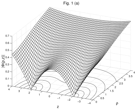
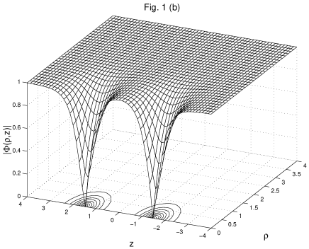
FIG. 1.: The modulus of the Higgs field as a function of $\rho$ and $z$ for $\lambda=0$ (a) and $\lambda=1$ (b)

In Fig. 2 we show the energy density of the monopole-antimonopole solution as a function of the coordinates $\rho=\sqrt{x^{2}+y^{2}}$ and $z$ for $\lambda=0$ and $\lambda=1$. At the locations of the zeros of the Higgs field the energy density possesses maxima. For $\lambda=1$ the maxima are more pronounced compared to the case of vanishing $\lambda$. At large distances from the origin the energy density vanishes like $O(r^{-6})$. For intermediate distances from the origin the shape of equal energy density surfaces looks like a dumb-bell. For smaller distances the dumb-bell splits into two surfaces.

Near the locations of the zeros of the Higgs field the equal energy density surfaces assume a shape close to a sphere, centered at the location of the respective zero. This presents further support for the conclusion, that at the two zeros of the Higgs field a monopole and an antimonopole are located, which can be clearly distinguished from each other, and which together form a bound state. This is in contrast to the axially symmetric charge-2 multimonopole solution, where the individual monopoles cannot be distinguished, and where, in fact, the Higgs field has only one (double) zero.

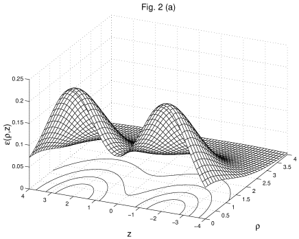
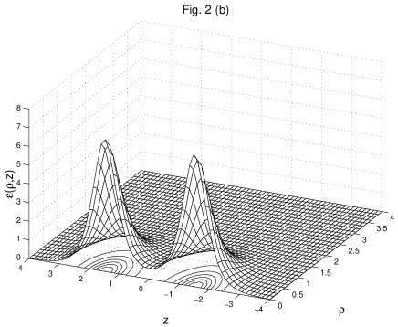
FIG. 2.: The the dimensionless energy density as a function of $\rho$ and $z$ for $\lambda=0$ (a) and $\lambda=1$ (b)

Considering finally the electromagnetic properties of the monopole-antimonopole solution, we observe, that the dimensionless dipole moment $C_{\rm\bf m}$ decreases monotonically with increasing $\lambda$ (see Table 1).

VI Conclusions

We have considered static axially symmetric solutions of the $SU(2)$ Yang-Mills-Higgs model, residing in the vacuum sector. These solutions represent monopole-antimonopole pairs. The modulus of the Higgs field possesses zeros at the locations of the monopole and antimonopole. Clearly distinguished from each other, the monopole and antimonopole together form a bound state, which carries a magnetic dipole moment and net zero magnetic charge. However, this bound state is unstable, corresponding to a saddle point [13, 14].

We have constructed the monopole-antimonopole solutions numerically for various values of the coupling constant $\lambda$, representing the strength of the Higgs potential. With increasing $\lambda$, the energy $E$ of the pair and the ratio $E/E_{\inf}$ increase and the distance $d$ between monopole and antimonopole as well as the magnetic dipole moment $C_{\rm m}$ decrease, while the energy density becomes more localized around the monopole and antimonopole locations.

In the BPS limit, the $SU(2)$ monopole-antimonopole solution does not satisfy the first order Bogomol’nyi equations [14]. Hopefully, the numerical solution will be of help in constructing this non-Bogomol’nyi solution analytically. Recently also non-Bogomol’nyi $SU(N)$ BPS solutions, corresponding to monopole-antimonopole configurations, have been found [20]. These solutions, however, are spherically symmetric.

Acknowledgments

B. K. was supported by Forbairt grant SC/97-636.

VII Appendix A

At first glance it seems to be obvious, that the second term in Eq. (53) does not contribute to the surface integral, because it is the curl of the “gauge field” $\tilde{A}_{\mu}=Tr\{\hat{\Phi}A_{\mu}\}$. However, $\hat{\Phi}$ is not continuous on the $z$-axis and introduces a singularity in the “gauge field” $\tilde{A}_{\mu}$; its curl may contain $\delta$-functions if the singularity is strong enough.

To examine the singularity we expand the functions near the singular point $\vec{r}_{s}=(0,0,z_{0})$,

$$\Phi_{1} = f_{0}+f_{2}\sin^{2}\theta\ ,\ \ \Phi_{2}\ =\ f_{1}\sin\theta\ ,\ \ \ \ f_{0}=c_{0}(z-z_{0})$$ (74)

$$\tilde{\Phi}_{1} = \sin\theta(f_{1}+2f_{0})\ ,\ \ \tilde{\Phi}_{2}=f_{0}+\sin^{2}\theta(f_{2}-2(f_{0}+f_{1}))$$ (75)

$$H_{3} = \sin\theta H_{31}\ ,\ \ 1-H_{4}\ =\ H_{40}+\sin^{2}\theta H_{42}\ ,$$ (76)

where $c_{0}$, $f_{1}$, $f_{2}$, $H_{31}$, $H_{40}$ and $H_{42}$ are constants. This leads to

$$\cos\alpha\ =\ \sin\theta\frac{f_{1}+2f_{0}}{\sqrt{f_{0}^{2}+\sin^{2}\theta f_{1}^{2}}}\ ,\ \ \sin\alpha\ =\ \frac{f_{0}+\sin^{2}\theta(f_{2}-2(f_{0}+f_{1}))}{\sqrt{f_{0}^{2}+\sin^{2}\theta f_{1}^{2}}}\ ,\ \$$ (78)

$$\tilde{A}_{x}\ =\ \frac{2y}{z}\frac{H_{31}f_{0}+H_{40}f_{1}}{\sqrt{z^{2}f_{0}^{2}+(x^{2}+y^{2})(f_{0}^{2}+f_{1}^{2})}}\ ,\ \ \tilde{A}_{y}\ =\ -\frac{2x}{z}\frac{H_{31}f_{0}+H_{40}f_{1}}{\sqrt{z^{2}f_{0}^{2}+(x^{2}+y^{2})(f_{0}^{2}+f_{1}^{2})}}\ .$$ (79)

Next we define $\bar{z}=z-z_{0}$ and keep only terms linear (quadratic under the square root) in $x$, $y$, $\bar{z}$,

$$\tilde{A}_{x}=2\frac{y}{z_{0}}\frac{H_{40}f_{1}}{\sqrt{c_{0}^{2}z_{0}^{2}\bar{z}^{2}+f_{1}^{2}(x^{2}+y^{2})}}\ ,\ \ \tilde{A}_{y}=-2\frac{x}{z_{0}}\frac{H_{40}f_{1}}{\sqrt{c_{0}^{2}z_{0}^{2}\bar{z}^{2}+f_{1}^{2}(x^{2}+y^{2})}}\ .$$ (81)

Now we introduce spherical coordinates $x=\bar{r}\sin\bar{\theta}\cos\bar{\varphi}$, $y=\bar{r}\sin\bar{\theta}\sin\bar{\varphi}$, $\bar{z}=\bar{r}\cos\bar{\theta}$ centered at the singular point. With respect to these coordinates the components of the “gauge field” become

$$\tilde{A}_{\bar{r}}=0\ ,\ \ \tilde{A}_{\bar{\theta}}=0\ ,\ \ \tilde{A}_{\bar{\varphi}}=-2\sin^{2}\bar{\theta}\frac{\bar{r}}{z_{0}}\frac{H_{40}f_{1}}{\sqrt{c_{0}^{2}z_{0}^{2}+\sin^{2}\bar{\theta}(f_{1}^{2}-c_{0}^{2}z_{0}^{2})}}\ .$$ (82)

Then we find for the curl

$$\tilde{F}_{\theta\varphi}=-\frac{2\bar{r}}{z_{0}}\partial_{\theta}\left\{\sin^{2}\bar{\theta}\frac{H_{40}f_{1}}{\sqrt{c_{0}^{2}z_{0}^{2}+\sin^{2}\bar{\theta}(f_{1}^{2}-c_{0}^{2}z_{0}^{2})}}\right\}\ .$$ (83)

Consequently the surface integral $\int_{0}^{2\pi}\int_{0}^{\pi}\tilde{F}_{\theta\varphi}d\theta d\varphi$ over a sphere centered at the singular point vanishes. Thus the singularity of the “gauge field” $\tilde{A}_{\mu}$ is too weak to introduce $\delta$-functions in the electromagnetic field strength tensor ${\cal F}_{\mu\nu}$.

REFERENCES

• [1] G. ‘t Hooft, Magnetic monopoles in unified gauge theories, Nucl. Phys.  B79 (1974) 276.
• [2] A. M. Polyakov, Particle spectrum in quantum field theory, JETP Lett. 20 (1974) 194.
• [3] M. K. Prasad and C. M. Sommerfield, Exact solutions for the ‘t Hooft monopole and the Julia-Zee dyon, Phys. Rev. Lett. 35 (1975) 760.
• [4] E. B. Bogomol’nyi and M. S. Marinov, Sov. J. Nucl. Phys. 23 (1976) 357.
• [5] E. J. Weinberg and A. H. Guth, Nonexistence of spherically symmetric monopoles with multiple magnetic charge, Phys. Rev. D 14 (1976) 1660.
• [6] C. Rebbi and P. Rossi, Multimonopole solutions in the Prasad-Sommerfield limit, Phys. Rev. D 22 (1980) 2010.
• [7] R. S. Ward, A Yang-Mills-Higgs monopole of charge 2, Commun. Math. Phys. 79 (1981) 317.
• [8] P. Forgacs, Z. Horvarth and L. Palla, Exact multimonopole solutions in the Bogomolny-Prasad-Sommerfield limit, Phys. Lett. 99B (1981) 232;
Non-linear superposition of monopoles, Nucl. Phys. B192 (1981) 141.
• [9] M. K. Prasad, Exact Yang-Mills Higgs monopole solutions of arbitrary charge, Commun. Math. Phys. 80 (1981) 137;
M. K. Prasad and P. Rossi, Construction of exact multimonopole solutions, Phys. Rev. D 24 (1981) 2182.
• [10] see e.g. P. M. Sutcliffe, BPS Monopoles, Int. J. Mod. Phys. A 12 (1997) 4663;
C. J. Houghton, N. S. Manton and P. M. Sutcliffe, Rational Maps, Monopoles and Skyrmions, Nucl. Phys. B 510 (1998) 507.
• [11] E. B. Bogomol’nyi, Sov. J. Nucl. Phys. 24 (1976) 449.
• [12] B. Kleihaus, J. Kunz and D. H. Tchrakian, Interaction energy of ’t Hooft-Polyakov monopoles, Mod. Phys. Lett. A13 (1998) 2523.
• [13] C. H. Taubes, The existence of a non-minimal solution to the SU(2) Yang-Mills-Higgs equations on $R^{3}$. Part I, Commun. Math. Phys. 86 (1982) 257;
Part II, Commun. Math. Phys. 86 (1982) 299.
• [14] Bernhard Rüber, Eine axialsymmetrische magnetische Dipollösung der Yang-Mills-Higgs-Gleichungen, Thesis, University of Bonn 1985.
• [15] F. Klinkhamer, Construction of a new electroweak sphaleron, Nucl. Phys. B410 (1993) 343.
• [16] Y. Brihaye and J. Kunz, On axially symmetric solutions in the electroweak theory, Phys. Rev. D 50 (1994) 1051.
• [17] Note the difference between the gauge transformation matrix ${\bf g}=\exp\{-i\frac{\varphi}{2}\tau_{3}\}\exp\{i\theta\tau_{2}\}\exp\{-i\frac{\varphi}{2}\tau_{3}\}$, and the corresponding matrix ${\bf g}^{(Q=1)}=\exp\{-i\frac{\varphi}{2}\tau_{3}\}\exp\{i\frac{\theta}{2}\tau_{2}\}\exp\{-i\frac{\varphi}{2}\tau_{3}\}$, which transforms the Higgs field of the charge-1 monopole into a constant. The former one is regular on the $z$-axis (except at $z=0$), whereas the latter one leads to a singularities along the negative $z$-axis.
• [18] B. Kleihaus, The regularity of static axially symmetric solutions in $SU(2)$ Yang-Mills-dilaton theory, Phys. Rev. D 59 (1999),125001.
• [19] W. Schönauer and R. Weiß, J. Comput. Appl. Math. 27, 279 (1989) 279; M. Schauder, R. Weiß and W. Schönauer, The CADSOL Program Package, Universität Karlsruhe, Interner Bericht Nr. 46/92 (1992).
• [20] T. Ioannidou and P. M. Sutcliffe, Non-Bogomol’nyi SU(N) BPS Monopoles, hep-th/9905169.