Abstract
The structures in target space geometry that correspond to conformally invariant boundary conditions in WZW theories are determined both by studying the scattering of closed string states and by investigating the algebra of open string vertex operators. In the limit of large level, we find branes whose world volume is a regular conjugacy class or, in the case of symmetry breaking boundary conditions, a ‘twined’ version thereof. In particular, in this limit one recovers the commutative algebra of functions over the brane world volume, and open strings connecting different branes disappear. At finite level, the branes get smeared out, yet their approximate localization at (twined) conjugacy classes can be detected unambiguously.
As a by-product, it is demonstrated how the pentagon identity and tetrahedral symmetry imply that in any rational conformal field theory the structure constants of the algebra of boundary operators coincide with specific entries of fusing matrices.

1 Introduction

Conformally invariant boundary conditions in two-dimensional conformal field theories have recently attracted renewed attention. By now, quite a lot of information on such boundary conditions is available in the algebraic approach, including boundary conditions that do not preserve all bulk symmetries. In many cases, the conformal field theory of interest has also a description as a sigma model with target space $M$. It is then tempting to ask what the geometrical interpretation of these boundary conditions might be in terms of submanifolds (and vector bundles on them or, more generally, sheaves) of $M$. Actually, this question makes an implicit assumption that is not really justified: It is not the classical (commutative) geometry of the target $M$ that matters, but rather a non-commutative version [1] of it.

In the present note, we investigate the special case of WZW conformal field theories. For most of the time we restrict our attention to the case where the torus partition function is given by charge conjugation. Then the classical target space is a real simple compact connected and simply connected Lie group manifold $G$. In particular, the underlying manifold is parallelizable, i.e. its tangent bundle is a trivial bundle.

The latter property of Lie groups will allow us to apply methods that were developped in [2], by which geometric features of the D-brane solutions of supergravity in flat 10-dimensional space-time were recovered from the boundary state for a free conformal field theory. The basic idea of that approach was to compute the vacuum expectation value of the bulk field that corresponds to the closed string state

$$\alpha^{\mu}_{-1}\,\tilde{\alpha}^{\nu}_{-1}|q\rangle\raisebox{0.70007pt}{$\scriptstyle\otimes$}|\tilde{q}\rangle$$ (1.1)

on a disk with a boundary condition $\beta$ of interest. Here our convention is that quantities without a tilde correspond to left-movers, while those with a tilde correspond to right-movers. The operator $\alpha^{\mu}_{n}$ is the $n$th mode of the $\mathfrak{u}(1)$ current in the $\mu$-direction of the free conformal field theory. The symmetric traceless part of the state (1.1) corresponds to the graviton, the antisymmetric part of the state to the Kalb–Ramond field, and the trace to the dilaton, all of momentum $q$.

Let us explain the rationale behind this prescription. At first sight it might seem more natural to employ graviton scattering in the background of a brane for exploring the geometry. This would correspond, in leading order of string perturbation theory, to the calculation of a two-point correlation function for two bulk fields on the disk. However, by factorization of bulk fields such an amplitude is related to (a sum of) products of three-point functions on the sphere with one-point functions on the disk. Since the former amplitude is completely independent of the boundary conditions, all information on a boundary condition that can be obtained by use of bulk fields will therefore be obtainable from correlators involving a single bulk field. Similar factorization arguments also encourage us to concentrate on world sheets with the topology of a disk.

The idea of testing boundary conditions with vacuum expectation values of bulk fields finds an additional justification in the following reasoning. In terms of classical geometry, boundary conditions are related to vector bundles over submanifolds of the target manifold $M$, the Chan–Paton bundles. Such bundles, in turn, should be regarded as modules over the ring ${\cal F}(M)$ of functions on $M$. Heuristically, we may interpret the algebra of (certain) bulk fields as a quantized version of ${\cal F}(M)$. The expectation values of the bulk fields on a disk then describe how the algebra of bulk fields is represented on the boundary operators or, more precisely, on the subspace of boundary operators that are descendants of the vacuum field. (As a side remark we mention that boundary conditions are indeed most conveniently described in terms of suitable classifying algebras. These encode aspects of the action of the algebra of bulk operators on boundary operators.)

The relevant information for computing the one-point functions on a disk with boundary condition $\beta$ is encoded in a boundary state ${\cal B}_{\beta}$, which is a linear functional

$${\cal B}_{\beta}:\quad\bigoplus_{q,\tilde{q}}\,{\cal H}_{q}\,{\otimes}\,{\cal H}_{\tilde{q}}\to{\mathbb{C}}$$ (1.2)

on the space of closed string states. (For an uncompactified free boson, the left- and right-moving labels of the primary fields are related as $\tilde{q}\,{=}\,q$.) We are thus led to compute the function

$${\rm G}_{\beta}^{\mu\nu}(q):={\cal B}_{\beta}(\alpha^{\mu}_{-1}\tilde{\alpha}^{\nu}_{-1}|q\rangle\raisebox{0.70007pt}{$\scriptstyle\otimes$}|\tilde{q}\rangle)\,.$$ (1.3)

Using the explicit form of the boundary state, this quantity has been determined in [2]. Upon Fourier transformation, it gives rise to a function $\tilde{\rm G}_{\beta}^{\mu\nu}(x)$ on position space. It has been shown that the symmetric traceless part of the function ${\rm G}_{\beta}$ reproduces the vacuum expectation value of the graviton in the background of a brane, while the antisymmetric part gives the Kalb–Ramond field, and the trace the dilaton.

In order to see how these findings generalize to the case of (non-abelian) WZW theories, let us examine the structural ingredients that enter in these calculations. Boundary states can be constructed for arbitrary conformal field theories, in particular for WZW models. Moreover, since group manifolds are parallelizable, it is also straightforward to generalize the oscillator modes $\alpha^{\nu}_{n}$: they are to be replaced by the corresponding modes $J^{a}_{n}$ of the non-abelian currents $J^{a}(z)$. Here the upper index $a$ ranges over a basis of the Lie algebra of $G$, $a\,{=}\,1,2,...\,,\dim G$, and $n\,{\in}\,{\mathbb{Z}}$. Together with a central element $K$, these modes span an untwisted affine Lie algebra ${\mathfrak{g}}$, according to

$$[J^{a}_{n},J^{b}_{m}]=\sum_{c}f^{ab}_{\;\ c}\,J^{c}_{n+m}+n\,\kappa^{ab}\delta_{n+m,0}\,K\,.$$ (1.4)

Here $f^{ab}_{\;\ c}$ and $\kappa^{ab}$ are the structure constants and Killing form, respectively, of the finite-dimensional simple Lie algebra $\bar{\mathfrak{g}}$ whose compact real form is the Lie algebra of the Lie group manifold $G$. Notice that the generators of the form $J_{0}^{a}$ form a finite-dimensional subalgebra, called the horizontal subalgebra, which can (and will) be identified with $\bar{\mathfrak{g}}$.

We finally need to find the correct generalization of the state $|q\rangle$. To this end we note that $|q\rangle$ is the vector in the Fock space of charge $q$ with lowest conformal weight. For WZW theories, instead of this Fock space, we have to consider the following space. First, we must choose a non-negative integer value $k$ for the level, i.e., the eigenvalue of the central element $K$. The space of physical states of the WZW theory with charge conjugation modular invariant is then the direct sum

$$\bigoplus_{\lambda\in P_{k}}{\cal H}_{\lambda}\,{\otimes}\,{\cal H}_{\lambda^{\!+}_{\phantom{i}}}\,,$$ (1.5)

where ${\cal H}_{\lambda}$ is the irreducible integrable highest weight module of ${\mathfrak{g}}$ at level $k$ with highest weight $\lambda$, and $P_{k}$ is the (finite) set of integrable weights $\lambda$ of ${\mathfrak{g}}$ at level $k$. Every such ${\mathfrak{g}}$-weight $\lambda$ corresponds to a unique weight of the horizontal subalgebra $\bar{\mathfrak{g}}$ (which we denote again by $\lambda$), which is the highest weight of a finite-dimensional $\bar{\mathfrak{g}}$-representation. However, for finite level $k$, not all such highest weights of $\bar{\mathfrak{g}}$ appear; this truncation will have important consequences later on.

Unlike in the case of Fock modules, the subspace of states of lowest conformal weight in the module ${\cal H}_{\lambda}$ is not one-dimensional any longer. Rather, it constitutes the irreducible finite-dimensional module $\bar{\cal H}_{\lambda}$ of the horizontal subalgebra $\bar{\mathfrak{g}}$. Therefore in place of the function (1.3) we now consider

$${\rm G}_{\beta}^{ab}(v\raisebox{0.70007pt}{$\scriptstyle\otimes$}\tilde{v}):={\cal B}_{\beta}(J^{a}_{-1}\tilde{J}^{b}_{-1}\,|v\rangle\raisebox{0.70007pt}{$\scriptstyle\otimes$}|\tilde{v}\rangle)$$ (1.6)

for

$$v\,\raisebox{0.70007pt}{$\scriptstyle\otimes$}\,\tilde{v}\in\bigoplus_{\lambda\in P_{k}}\bar{\cal H}_{\lambda}\,{\otimes}\,\bar{\cal H}_{\lambda^{\!+}_{\phantom{i}}}\,.$$ (1.7)

As a matter of fact, one may also look at analogous quantities involving other modes $J^{a}_{n}$, or combinations of modes, or even without any mode present at all. It turns out that qualitatively their behavior is very similar to the functions (1.6); they all signal the presence of a defect at the same position in target space. Our results are therefore largely independent on the choice of the bulk field we use to test the geometry of the target.

The function ${\rm G}_{\beta}^{ab}$ can be determined from known results about boundary conditions in WZW models. This allows us to analyze WZW brane geometries via expectation values of bulk fields. Another approach to these geometries is via the algebra of boundary fields. While the second setup focuses on intrinsic properties of the brane world volume, the first perspective offers a natural way to study the embedding of the brane geometry into the target. Both approaches will be studied in this paper.

We organize our discussion as follows. In section 2 we compute the function ${\rm G}_{\beta}^{ab}$ for those boundary conditions which preserve all bulk symmetries. To relate this function to classical geometry of the group manifold $G$, we perform a Fourier transformation. We then find that the end points of open strings are naturally localized at certain conjugacy classes of the group $G$. At finite level $k$, the locus of the end points of the open string is, however, smeared out, though it is still well peaked at a definite regular rational conjugacy class. The absence of sharp localization at finite level $k$ shows that, even after having made the relation to classical geometry, the brane exhibits some intrinsic ‘fuzziness’. It should, however, be emphasized that at finite level the very concept of both the target space and the world volume of a brane as classical finite-dimensional manifolds are not really appropriate.

The algebra of boundary fields for symmetry preserving boundary conditions is analyzed in section 3. It can be shown that for any arbitrary rational conformal field theory the boundary structure constants are equal to world sheet duality matrices, the fusing matrices, according to

$$C_{\,\lambda\mu\,{\scriptscriptstyle L}\,\nu}^{\alpha\,{\scriptscriptstyle A}\,\beta\,{\scriptscriptstyle B}\,\gamma\,{\scriptscriptstyle C}}=\mbox{\large(}{\sf F}_{\!{{{\scriptscriptstyle L}}{\nu}{{\scriptscriptstyle C}}},{{{\scriptscriptstyle A}}{\beta^{+}_{\phantom{i}}}{{\scriptscriptstyle B}}}}\mbox{\large$[$}\!\!{\scriptstyle\begin{array}[]{c}{}\hfil\\[-13.58003pt] {\scriptstyle\lambda\;\,\;\mu}\\[-3.00995pt] {\scriptstyle\alpha^{+}_{\phantom{i}}\,\gamma}\\[-2.79996pt] \end{array}}\!\!\mbox{\large$]$}{\mbox{\large)}}^{*}\,.$$ (1.8)

Furthermore, we are able to show that in the limit of large $k$ the space of boundary operators approaches the space of functions on the brane world volume. In the same limit open strings connecting different conjugacy classes disappear, while such configurations are present at every finite value of the level.

In section 4 we discuss symmetry breaking boundary conditions in WZW theories for which the symmetry breaking is characterized through an automorphism $\omega$ of the horizontal subalgebra $\bar{\mathfrak{g}}$.  It turns out that the end points of open strings are then localized at twined conjugacy classes, that is, at sets of the form

$${\cal C}_{G}^{\omega}(h):=\{gh\omega(g)^{-1}\,|\,g\,{\in}\,G\}$$ (1.9)

for some $h\,{\in}\,G$. The derivation of our results on symmetry breaking boundary conditions requires generalizations of Weyl’s classical results on conjugacy classes. (The necessary tools, including a twined version of Weyl’s integration formula, are collected in appendix B.) In section 5, we extend our analysis to non-simply connected Lie groups. We find features that are familiar from the discussion of D-branes on orbifold spaces, such as fractional branes, and point out additional subtleties in cases where the action of the orbifold group is only projective.

2 Probing target geometry with bulk fields

We start our discussion with the example of boundary conditions that preserve all bulk symmetries. In this situation the correlators on a surface with boundaries are specific linear combinations of the chiral blocks on the Schottky double of the surface [3]. The boundary state describes the one-point correlators for bulk fields on the disk and, accordingly, it is a linear combination of two-point blocks on the Schottky cover of the disk, i.e., on the sphere. The latter – which in the present context of correlators on the disk also go under the name of Ishibashi states – are linear functionals

$$B_{\lambda}\,:\quad{\cal H}_{\lambda}\,{\otimes}\,{\cal H}_{\lambda^{\!+}_{\phantom{i}}}\to{\mathbb{C}}$$ (2.1)

that are characterized by the Ward identities

$$B_{\lambda}\circ\left(J^{a}_{n}\,\raisebox{0.70007pt}{$\scriptstyle\otimes$}\,{\bf 1}+{\bf 1}\,\raisebox{0.70007pt}{$\scriptstyle\otimes$}\,J^{a}_{-n}\right)=0\,.$$ (2.2)

Choosing an element $v\raisebox{0.70007pt}{$\scriptstyle\otimes$}\tilde{v}\,{\in}\,\bar{\cal H}_{\lambda}{\otimes}\bar{\cal H}_{\lambda^{\!+}_{\phantom{i}}}$, we can use the invariance property (2.2) and the commutation relations (1.4) to arrive at

$$\begin{array}[]{ll}B_{\lambda}(J^{a}_{-1}v\,\raisebox{0.70007pt}{$\scriptstyle\otimes$}\,J^{b}_{-1}\tilde{v})\!\!&=-B_{\lambda}(({\bf 1}\,\raisebox{0.70007pt}{$\scriptstyle\otimes$}\,J^{a}_{1}J^{b}_{-1})\,(v\raisebox{0.70007pt}{$\scriptstyle\otimes$}\tilde{v}))=-B_{\lambda}(({\bf 1}\,\raisebox{0.70007pt}{$\scriptstyle\otimes$}\,[J^{a}_{1},J^{b}_{-1}])\,(v\raisebox{0.70007pt}{$\scriptstyle\otimes$}\tilde{v}))\\ {}\\[-6.00006pt] &=-\displaystyle\sum_{c}f^{ab}_{\;\ c}\,B_{\lambda}(v\,\raisebox{0.70007pt}{$\scriptstyle\otimes$}\,J^{c}_{0}\tilde{v})-\kappa^{ab}k\,B_{\lambda}(v\raisebox{0.70007pt}{$\scriptstyle\otimes$}\tilde{v})\,.\end{array}$$ (2.3)

There is one symmetry preserving boundary condition for each primary field $\alpha$ in the theory [4]. The coefficients in the expansion of the boundary states with respect to the boundary blocks are given by the so-called (generalized) quantum dimensions:

$${\cal B}_{\alpha}=\sum_{\lambda\in P_{k}}\frac{S_{\lambda,\alpha}}{S_{\Omega,\alpha}}\,B_{\lambda}\,.$$ (2.4)

Here $S$ is the modular S-matrix of the theory and $\Omega$ refers to the vacuum primary field. To write the state (2.4) in a more convenient form, we use the fact that the generalized quantum dimensions are given by the values of the $\bar{\mathfrak{g}}$-character of $\bar{\cal H}_{\lambda}$ at specific elements $y_{\alpha}$ of the Cartan subalgebra of the horizontal subalgebra $\bar{\mathfrak{g}}$ or, equivalently, by the values of the $G$-character of $\bar{\cal H}_{\lambda}$ at specific elements $h_{\alpha}$ of the maximal torus of the group $G$. Concretely, we have

$$S_{\lambda,\alpha}/S_{\Omega,\alpha}=\raisebox{1.49994pt}{$\chi$}_{\lambda}(h_{\alpha})$$ (2.5)

with

$$\raisebox{1.49994pt}{$\chi$}_{\lambda}(h):={\rm tr}_{\bar{\cal H}_{\lambda}}R_{\lambda}(h)$$ (2.6)

and

$$h_{\alpha}:=\exp(2\pi{\rm i}y_{\alpha})\quad{\rm with}\quad y_{\alpha}:=\mbox{\large$\frac{\alpha+\rho}{k+g^{\scriptscriptstyle\vee}}$}$$ (2.7)

for any level $k$ and $\bar{\mathfrak{g}}$-weight $\alpha$. In formula (2.7), $\rho$ denotes the Weyl vector (i.e., half the sum of all positive roots) of $\bar{\mathfrak{g}}$ and $g^{\scriptscriptstyle\vee}$ is the dual Coxeter number. The boundary state thus reads

$${\cal B}_{\alpha}=\sum_{\lambda\in P_{k}}\raisebox{1.49994pt}{$\chi$}_{\lambda}(h_{\alpha})\,B_{\lambda}\,.$$ (2.8)

The function ${\rm G}_{\alpha}^{ab}$ defined in formula (1.6) is then found to be

$${\rm G}^{ab}_{\alpha}(v\raisebox{0.70007pt}{$\scriptstyle\otimes$}\tilde{v})=-\raisebox{1.49994pt}{$\chi$}_{\lambda}(h_{\alpha})\left[B_{\lambda}(v\,\raisebox{0.70007pt}{$\scriptstyle\otimes$}\,[J^{a}_{0},J^{b}_{0}]\tilde{v})+\kappa^{ab}k\,B_{\lambda}(v\raisebox{0.70007pt}{$\scriptstyle\otimes$}\tilde{v})\right]$$ (2.9)

for $v\raisebox{0.70007pt}{$\scriptstyle\otimes$}\tilde{v}\,{\in}\,\bar{\cal H}_{\lambda}{\otimes}\bar{\cal H}_{\lambda^{\!+}_{\phantom{i}}}$.

We recall that the group character $\chi$ is a class function, i.e. a function that is constant on the conjugacy classes

$${\cal C}_{G}(h):=\{ghg^{-1}\,|\,g\,{\in}\,G\}$$ (2.10)

of $G$. It is therefore quite natural to associate to a symmetry preserving boundary condition the conjugacy class ${\cal C}_{G}(h_{\alpha})$ of the Lie group $G$ that contains the element $h_{\alpha}$. We would like to emphasize that ${\cal C}_{G}(h_{\alpha})$ is always a regular conjugacy class, that is, the stabilizer of $h_{\alpha}$ under conjugation is just the unique maximal torus containing this element.

Our next task is to perform the analogue of the Fourier transformation between ${\rm G}^{\mu\nu}$ and $\tilde{\rm G}^{\mu\nu}$ in [2]. To this end we employ the fact that left and right translation on the group manifold $G$ give two commuting actions of $G$ on the space ${\cal F}(G)$ of functions on $G$ and thereby turn this space into a $G$-bimodule. By the Peter–Weyl theorem, ${\cal F}(G)$ is isomorphic, as a $G$-bimodule, to an infinite direct sum of tensor products of irreducible modules, namely

$${\cal F}(G)\,\cong\,\bigoplus_{\lambda\in P}\bar{\cal H}_{\lambda}\otimes\bar{\cal H}_{\lambda^{\!+}_{\phantom{i}}}\,.$$ (2.11)

Here $P\,{\equiv}\,P_{k=\infty}$ is the set of all highest weights of finite-dimensional irreducible $\bar{\mathfrak{g}}$-modules. We may identify the conjugate module $\bar{\cal H}_{\lambda^{\!+}_{\phantom{i}}}$ with the dual of $\bar{\cal H}_{\lambda}$. Then the isomorphism (2.11) sends $v\raisebox{0.70007pt}{$\scriptstyle\otimes$}\tilde{v}\,{\in}\,\bar{\cal H}_{\lambda}{\otimes}\bar{\cal H}_{\lambda^{\!+}_{\phantom{i}}}$ to the function $f$ on $G$ given by

$$f(g)=\tilde{v}(R_{\lambda}(g)v)\equiv\langle\tilde{v}|R_{\lambda}(g)|v\rangle$$ (2.12)

for all $g\,{\in}\,G$. Using the scalar product on ${\cal F}(G)$, we can therefore associate to every linear functional $\beta{:}\;{\cal F}\,{\to}\,{\mathbb{C}}$ a function (respectively, in general, a distribution) $\tilde{\beta}$ on the group manifold by the requirement that

$$\beta(v\raisebox{0.70007pt}{$\scriptstyle\otimes$}\tilde{v})=\int_{G}\!{\rm d}g\,\tilde{\beta}(g)^{*}\,\langle\tilde{v}|R_{\lambda}(g)|v\rangle$$ (2.13)

for $v\raisebox{0.70007pt}{$\scriptstyle\otimes$}\tilde{v}\,{\in}\,\bar{\cal H}_{\lambda}{\otimes}\bar{\cal H}_{\lambda^{\!+}_{\phantom{i}}}$. After introducing dual bases $\{v_{i}\}$ of $\bar{\cal H}_{\lambda}$ and $\{\tilde{v}_{j}\}$ of $\bar{\cal H}_{\lambda^{\!+}_{\phantom{i}}}$, the orthonormality relations for representation functions then allow us to write

$$\tilde{\beta}(g)=\sum_{\lambda\in P}\sum_{i,j}\beta(v_{i}\raisebox{0.70007pt}{$\scriptstyle\otimes$}\tilde{v}_{j})^{*}\,\langle\tilde{v}_{j}|R_{\lambda}(g)|v_{i}\rangle\,.$$ (2.14)

According to (1.7), at finite level we have to deal with the finite-dimensional truncations

$${\cal F}_{k}(G):=\bigoplus_{\lambda\in P_{k}}\bar{\cal H}_{\lambda}\,{\otimes}\,\bar{\cal H}_{\lambda^{\!+}_{\phantom{i}}}$$ (2.15)

of the space (2.11) of functions on $G$. For every $k$, the space ${\cal F}_{k}(G)$ can be regarded as a subspace of ${\cal F}(G)$. We will do so from now on; thereby we arrive at a picture that is close to classical intuition. The level-dependent truncation (2.15) constitutes, in fact, one of the basic features of a WZW conformal field theory. (This is a typical effect in interacting rational conformal field theories, which does not have an analogue for flat backgrounds.)

Next we relate the linear function ${\rm G}^{ab}$ on ${\cal F}_{k}$ to a function $\tilde{\rm G}^{ab}$ on the group manifold $G$ by the prescription

$$\tilde{\rm G}^{ab}(g):=\sum_{\lambda\in P_{k}}\sum_{i,j}{\rm G}^{ab}(v_{i}\raisebox{0.70007pt}{$\scriptstyle\otimes$}\tilde{v}_{j})^{*}\,\langle\tilde{v}_{j}|R_{\lambda}(g)|v_{i}\rangle$$ (2.16)

for $g\,{\in}\,G$. By direct calculation we find

$$\begin{array}[]{ll}{\rm G}^{ab}(g)\!\!&=-\displaystyle\sum_{\lambda\in P_{k}}\mbox{\large(}\kappa^{ab}k\,\mbox{\large$\frac{S_{\lambda,\alpha}^{*}}{S_{\Omega,\alpha}}$}\,{\rm tr}_{\bar{\cal H}_{\lambda}}R_{\lambda}(g)+\sum_{c}f^{ab}_{\;\ c}\,\mbox{\large$\frac{S_{\lambda,\alpha}^{*}}{S_{\Omega,\alpha}}$}\,{\rm tr}_{\bar{\cal H}_{\lambda}}J^{c}R_{\lambda}(g)\mbox{\large)}\\ {}\\[-8.00003pt] &=\displaystyle-\kappa^{ab}k\sum_{\lambda\in P_{k}}\raisebox{1.49994pt}{$\chi$}_{\lambda}(h_{\alpha})^{*}\,\raisebox{1.49994pt}{$\chi$}_{\lambda}(g)-\sum_{\lambda\in P_{k}}\raisebox{1.49994pt}{$\chi$}_{\lambda}(h_{\alpha})^{*}\,{\rm tr}_{\bar{\cal H}_{\lambda}}[J^{a},J^{b}]R_{\lambda}(g)\,.\end{array}$$ (2.17)

In analogy with the situation for flat backgrounds [2] we are led to the following interpretation of this result. The first term in the expression (2.17) is symmetric and hence describes the vacuum expectation value of dilaton and metric that is induced by the presence of the brane, while the second term, which is antisymmetric, corresponds to the vacuum expectation value for the Kalb–Ramond field.

To proceed, we introduce, for every $k\,{\in}\,{\mathbb{Z}}_{>0}$, a function $\varphi_{k}$ on $G\,{\times}\,G$ by

$$\varphi_{k}(g,h):=\sum_{\lambda\in P_{k}}\raisebox{1.49994pt}{$\chi$}_{\lambda}(g)\,\raisebox{1.49994pt}{$\chi$}_{\lambda}(h)^{*}\,.$$ (2.18)

In the limit $k\,{\to}\,\infty$ the integral operator associated to $\varphi_{k}$ reduces to the $\delta$-distribution on the space of conjugacy classes. Indeed, because of $\lim_{k\to\infty}P_{k}\,{=}\,P$, for every class function $f$ on $G$ we have

$$\int_{G}\!{\rm d}h\,\lim_{k\to\infty}\varphi_{k}(g,h)\,f(h)=f(g)\,,$$ (2.19)

which is a consequence of the general relation

$$\int_{G}\!{\rm d}g\,\raisebox{1.49994pt}{$\chi$}_{V}(g)^{*}\,\raisebox{1.49994pt}{$\chi$}_{W}(g)=\dim({\rm Hom}_{G}(V,W))$$ (2.20)

valid for any two $G$-modules $V,\,W$. Comparison with the result (2.17) thus shows that, in the limit of infinite level, the brane is localized at the conjugacy class ${\cal C}_{G}(h_{\alpha})$ of $G$. It is worth emphasizing, however, that this holds true only in that limit. In contrast, at finite level, the brane world volume is not sharply localized on the relevant conjugacy class ${\cal C}_{G}(h_{\alpha})$. Rather, it gets smeared out or, in more fancy terms, its localization is on a ‘fuzzy’ version of a conjugacy class. Nevertheless, already at very small level the localization is sufficiently sharp to indicate unambiguously what remains in the limit.

For concreteness, we display a few examples for boundary conditions with ${\mathfrak{g}}\,{=}\,\mathfrak{sl}(2)$ in figure 1. The functions of interest are

$$f_{k,\alpha}(h):={\cal N}\,J(h)\,\mbox{\Large$|$}\!\sum_{\lambda\in P_{k}}\raisebox{1.49994pt}{$\chi$}_{\lambda}(h_{\alpha})\,\raisebox{1.49994pt}{$\chi$}_{\lambda}(h)\mbox{\Large$|$}^{2}\,,$$ (2.21)

where $J$ is the weight factor in the Weyl integration formula (see (A.3) and (A.8)) and ${\cal N}$ is a normalization constant which is determined by the requirement that $\int_{T}{\rm d}h\,f(h)\,{=}\,1$. For $\mathfrak{sl}(2)$, we have $T\,{=}\,[0,2]$ and $J(z)\,{=}\,\sin^{2}(\pi z)$. The functions (2.21) are then given by

$$f_{k,x}(z)={\cal N}_{k,x}\,\mbox{\large(}\sum_{\lambda=0}^{k}\sin((\lambda{+}1)\pi x)\,\sin(\pi z){\mbox{\large)}}^{2}$$ (2.22)

for $z\,{\in}\,[0,1)$, where $k\,{\in}\,{\mathbb{Z}}_{>0}$ and $x\,{=}\,(\mu{+}1)/(k{+}2)$ with $\mu\,{\in}\,\{0,1,...\,,k\}$. The examples plotted in figure 1 are for conjugacy classes $x\,{=}\,1/6$ and $1/2$ and for levels $k\,{=}\,4,\,10$ and $28$.

Closer inspection of the $\mathfrak{sl}(2)$ data also shows that the sharpness of the localization scales with $k{+}g^{\scriptscriptstyle\vee}$. More specifically, for any given conjugacy class $x$ and any fraction $p$ of $\kappa\,{=}\,(k{+}2)^{-1}$, the integrated density $I_{x,p}\,{:=}\int_{x-\kappa/p}^{x+\kappa/p}{\rm d}z\,f(z)$ depends only very weakly on the level. In fact, we have collected extensive numerical evidence that even after taking this rescaling into account, the localization improves when the level gets larger, i.e., that $I_{x,p}(k)$ is monotonically increasing with $k$. (The improvement is not spectacular, though. For instance, $I_{x=\kappa,1}$ rises from $.9829$ at $k\,{=}\,3$ to $.9889$ at $k\,{=}\,20$, and $I_{x=\kappa,3}$ rises from $.6063$ to $.6074$.)

Note in particular that all brane world volumes are concentrated on regular conjugacy classes, and that already at small level the overlap with the exceptional conjugacy classes (i.e., $x\,{=}\,0$ and $x\,{=}\,1$ for ${\mathfrak{g}}\,{=}\,\mathfrak{sl}(2)$) is negligible. Indeed, as is clearly exhibited by the last mentioned data, even the level-dependent allowed conjugacy classes that, at fixed level, are closest to an exceptional class (i.e., $x\,{=}\,\kappa$ for ${\mathfrak{g}}\,{=}\,\mathfrak{sl}(2)$) are not driven into the exceptional one in the infinite level limit. (Thus, in this respect, our findings do not agree with the prediction of the semi-classical analysis in [5] and in [6]. The origin of this discrepancy appears to be the absence of the shift $k\,{\mapsto}\,k{+}g^{\scriptscriptstyle\vee}$ in the classical setup. This shift occurs also naturally in other quantities like e.g. in character formulæ and conformal weights.) This result will be confirmed by the investigation of the algebra of boundary operators, to which we now turn our attention.

                                                                                

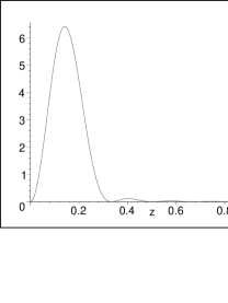
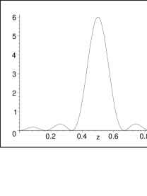
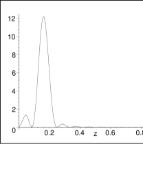
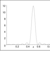
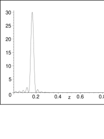
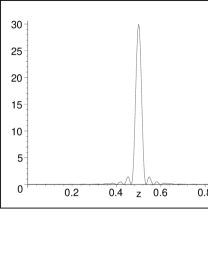
Figure 1: The function (2.22) for branes centered at the conjugacy classes $x\,{=}\,1/6$ and $x\,{=}\,1/2$ for levels $4,10,28$.

3 The algebra of boundary fields

In this section we focus our attention on the operator product algebra of (WZW-primary) boundary fields. As a first basic ingredient, we need to determine by which quantum numbers such a field is characterized. Boundary points are precisely those points of a surface that have a unique pre-image on its Schottky cover. Accordingly, on the level of chiral conformal field theory, boundary operators are characterized by a single primary label $\lambda$.  When all bulk symmetries are preserved, this label takes its values in the set of chiral bulk labels. (In the presence of symmetry breaking boundary conditions, the analysis has to be refined, see [7, 8].) Moreover, a boundary operator typically changes the boundary condition; therefore it carries two additional labels $\alpha,\beta$ which indicate the two conformally invariant boundary conditions at the two segments adjacent to the boundary insertion.

Boundary operators are therefore often written as $\Psi_{\;\lambda}^{\beta\,{\scriptscriptstyle\!}\,\alpha}(x)$. But, in fact, this is still not sufficient, in general. The reason is that field-state correspondence requires to associate to every  state that contributes to the partition function

$${\rm A}_{\alpha\,\beta}(t)=\sum_{\mu}{\rm A}_{\alpha\,\beta}^{\mu}\,\raisebox{1.49994pt}{$\chi$}_{\mu}(\mbox{\large$\frac{{\rm i}t}{2}$})$$ (3.1)

for an annulus with boundary conditions $\alpha$ and $\beta$ a separate boundary field. For symmetry preserving boundary conditions, the annulus coefficients ${\rm A}_{\alpha\,\beta}^{\mu}$ are known [4]  to coincide with fusion rule coefficients:

$${\rm A}_{\alpha\,\beta}^{\mu}={\rm N}_{\beta\mu}^{\ \ \alpha}\,.$$ (3.2)

The fusion rules ${\rm N}_{\beta\mu}^{\ \ \alpha}$ are not, in general, zero or one; as a consequence one must introduce another degeneracy label $A$, taking values in $\{1,2,...\,,{\rm N}_{\alpha^{+}_{\phantom{i}}\beta\mu}\}$ [7, 6, 9]. The complete labelling of boundary operators therefore looks like

$$\Psi_{\;\lambda}^{\beta\,{\scriptscriptstyle A}\,\alpha}(x)\,.$$ (3.3)

We remark in passing that in more complicated situations, like e.g. symmetry breaking boundary conditions [7] or non-trivial modular invariants [10], the degeneracy spaces relevant for the boundary operators still admit a representation theoretic interpretation that involves appropriate (sub-)bundles of chiral blocks.

The boundary fields satisfy an operator product expansion which schematically reads

$$\Psi_{\;\lambda}^{\alpha\,{\scriptscriptstyle A}\,\beta}(x)\,\Psi_{\;\mu}^{\beta\,{\scriptscriptstyle B}\,\gamma}(y)\,\sim\,\sum_{\nu}\sum_{L=1}^{{\rm N}_{\lambda\mu}^{\ \ \nu}}\sum_{C=1}^{{\rm N}_{\alpha\nu}^{\ \ \gamma}}C_{\,\lambda\mu\,{\scriptscriptstyle L}\,\nu}^{\alpha\,{\scriptscriptstyle A}\,\beta\,{\scriptscriptstyle B}\,\gamma\,{\scriptscriptstyle C}}\,[\Psi_{\;\nu}^{\alpha\,{\scriptscriptstyle C}\,\gamma}(y)+...\,]\,,$$ (3.4)

where $L\,{\in}\,\{1,2,...\,,{\rm N}_{\lambda\mu}^{\ \ \nu}\}$ labels a basis of the space of chiral couplings from $\lambda$ and $\mu$ to $\nu$. It turns out that for every (rational) conformal field theory, the structure constants $C_{\,\lambda\mu\,{\scriptscriptstyle L}\,\nu}^{\alpha\,{\scriptscriptstyle A}\,\beta\,{\scriptscriptstyle B}\,\gamma\,{\scriptscriptstyle C}}$ appearing here are nothing but suitable entries of fusing matrices ${\sf F}$:

$$C_{\,\lambda\mu\,{\scriptscriptstyle L}\,\nu}^{\alpha\,{\scriptscriptstyle A}\,\beta\,{\scriptscriptstyle B}\,\gamma\,{\scriptscriptstyle C}}=\mbox{\large(}{\sf F}_{\!{{{\scriptscriptstyle L}}{\nu}{{\scriptscriptstyle C}}},{{{\scriptscriptstyle A}}{\beta^{+}_{\phantom{i}}}{{\scriptscriptstyle B}}}}\mbox{\large$[$}\!\!{\scriptstyle\begin{array}[]{c}{}\hfil\\[-13.58003pt] {\scriptstyle\lambda\;\,\;\mu}\\[-3.00995pt] {\scriptstyle\alpha^{+}_{\phantom{i}}\,\gamma}\\[-2.79996pt] \end{array}}\!\!\mbox{\large$]$}{\mbox{\large)}}^{*}\,.$$ (3.5)

Indeed, recall that the fusing matrices describe the transition between the $s$- and the $t$-channel of four-point blocks; pictorially, in our conventions, this relation looks like

$$\begin{picture}(77.0,80.0)(0.0,66.0) \put(30.0,50.0){\line(0,1){30.0}} \put(30.0,80.0){\line(1,1){22.0}} \put(30.0,80.0){\line(-1,1){22.0}} \put(30.0,50.0){\line(1,-1){23.0}} \put(30.0,50.0){\line(-1,-1){23.0}} \put(30.0,60.0){\vector(0,-1){5.0}} \put(10.0,100.0){\vector(1,-1){5.0}} \put(10.0,30.0){\vector(1,1){5.0}} \put(50.0,100.0){\vector(-1,-1){5.0}} \put(50.0,30.0){\vector(-1,1){5.0}} \put(0.5,19.0){{$\scriptstyle\kappa$}} \put(0.5,104.0){{$\scriptstyle\lambda$}} \put(54.5,104.0){{$\scriptstyle\mu$}} \put(54.5,19.0){{$\scriptstyle\nu$}} \put(32.5,63.0){{$\scriptstyle\rho$}} \put(27.7,84.0){{$\scriptscriptstyle K$}} \put(27.7,42.5){{$\scriptscriptstyle L$}} \end{picture}=\;\sum_{\sigma}\sum_{M=1}^{{\rm N}_{\kappa\lambda}^{\ \ \sigma}}\sum_{N=1}^{{\rm N}_{\sigma\mu}^{\ \ \nu^{+}}}\ {\sf F}_{\!{{{\scriptscriptstyle K}}{\rho}{{\scriptscriptstyle L}}},{{{\scriptscriptstyle M}}{\sigma}{{\scriptscriptstyle N}}}}\mbox{\large$[$}\!\!{\scriptstyle\begin{array}[]{c}{}\hfil\\[-13.58003pt] {\scriptstyle\lambda\,\mu}\\[-3.00995pt] {\scriptstyle\kappa\,\nu}\\[-2.79996pt] \end{array}}\!\!\mbox{\large$]$}\ \cdot\begin{picture}(115.0,80.0)(11.0,50.0) \put(50.0,50.0){\line(1,0){30.0}} \put(50.0,50.0){\line(-1,1){22.0}} \put(50.0,50.0){\line(-1,-1){22.0}} \put(80.0,50.0){\line(1,1){22.0}} \put(80.0,50.0){\line(1,-1){22.0}} \put(70.0,50.0){\vector(1,0){5.0}} \put(30.0,70.0){\vector(1,-1){5.0}} \put(30.0,30.0){\vector(1,1){5.0}} \put(100.0,70.0){\vector(-1,-1){5.0}} \put(100.0,30.0){\vector(-1,1){5.0}} \put(19.6,20.5){{$\scriptstyle\kappa$}} \put(19.6,75.0){{$\scriptstyle\lambda$}} \put(106.0,75.0){{$\scriptstyle\mu$}} \put(106.0,20.5){{$\scriptstyle\nu$}} \put(63.0,51.5){{$\scriptstyle\sigma$}} \put(39.7,48.4){{$\scriptscriptstyle M$}} \put(83.9,48.4){{$\scriptscriptstyle N$}} \end{picture}$$ (3.6)

To establish the identity (3.5), we observe that the operator product coefficients $C_{\,\lambda\mu\,{\scriptscriptstyle L}\,\nu}^{\alpha\,{\scriptscriptstyle A}\,\beta\,{\scriptscriptstyle B}\,\gamma\,{\scriptscriptstyle C}}$ furnish a solution of the sewing constraint [11, 12] that arises from the two different factorizations of a correlation function of four boundary fields. Including all degeneracy labels, this sewing relation reads

$$\begin{array}[]{l}\displaystyle\sum_{E=1}^{{\rm N}_{\gamma\rho}^{\ \ \alpha}}C_{\,\kappa\lambda\,{\scriptscriptstyle K}\,\rho}^{\alpha\,{\scriptscriptstyle A}\,\beta\,{\scriptscriptstyle B}\,\gamma\,{\scriptscriptstyle E}}\,C_{\,\mu\nu\,{\scriptscriptstyle L}\,\rho^{+}_{\phantom{i}}}^{\gamma\,{\scriptscriptstyle C}\,\delta\,{\scriptscriptstyle D}\,\alpha\,{\scriptscriptstyle{E}}}\,C_{\,\rho\,\rho^{+}_{\phantom{i}}\;\Omega}^{\alpha\,{\scriptscriptstyle E}\,\gamma\,{\scriptscriptstyle{E}}\,\alpha}\\ {}\\[-13.99995pt] \mbox{\hskip 50.00008pt}=\displaystyle\sum_{\sigma}\sum_{M=1}^{{\rm N}_{\lambda\mu}^{\ \ \sigma}}\sum_{N=1}^{{\rm N}_{\kappa\sigma}^{\ \ \nu^{+}_{\phantom{i}}}}\sum_{F=1}^{{\rm N}_{\delta\sigma}^{\ \ \beta}}C_{\,\lambda\mu\,{\scriptscriptstyle M}\,\sigma}^{\beta\,{\scriptscriptstyle B}\,\gamma\,{\scriptscriptstyle C}\,\delta\,{\scriptscriptstyle F}}\,C_{\,\kappa\sigma\,{\scriptscriptstyle N}\,\nu^{+}_{\phantom{i}}}^{\alpha\,{\scriptscriptstyle A}\,\beta\,{\scriptscriptstyle F}\,\delta\,{\scriptscriptstyle{D}}}\,C_{\,\nu^{+}_{\phantom{i}}\,\nu\;\Omega}^{\alpha\,{\scriptscriptstyle{D}}\,\delta\,{\scriptscriptstyle D}\,\alpha}\cdot{\sf F}_{\!{{{\scriptscriptstyle M}}{\sigma}{{\scriptscriptstyle N}}},{{{\scriptscriptstyle K}}{\rho}{{\scriptscriptstyle L}}}}\mbox{\large$[$}\!\!{\scriptstyle\begin{array}[]{c}{}\hfil\\[-13.58003pt] {\scriptstyle\lambda\,\mu}\\[-3.00995pt] {\scriptstyle\kappa\,\nu}\\[-2.79996pt] \end{array}}\!\!\mbox{\large$]$}\,,\end{array}$$ (3.7)

where ${\sf F}\mbox{\large$[$}\!\!{\scriptstyle\begin{array}[]{c}{}\hfil\\[-13.58003pt] {\scriptstyle\lambda\,\mu}\\[-3.00995pt] {\scriptstyle\kappa\,\nu}\\[-2.79996pt] \end{array}}\!\!\mbox{\large$]$}$ is the fusing matrix which relates the two different factorizations. For WZW models, the fusing matrices coincide with the $6j$-symbols of the corresponding quantum group with deformation parameter a $k{+}g^{\scriptscriptstyle\vee}$th root of unity. The constraint (3.7) can be solved explicitly in full generality, without reference to the particular conformal field theory under investigation. First note that the structure constants $C_{\,\lambda\mu\,{\scriptscriptstyle L}\,\nu}^{\alpha\,{\scriptscriptstyle A}\,\beta\,{\scriptscriptstyle B}\,\gamma\,{\scriptscriptstyle C}}$ depend on six chiral and four degeneracy labels, so that their label structure is precisely the same as the one of the fusing matrices. The key observation is then to realize the similarity between the constraint (3.7) and the pentagon identity

$$\begin{array}[]{l}\displaystyle\sum_{{E}=1}^{{\rm N}_{\gamma\rho}^{\ \ \alpha}}{\sf F}_{\!{{{\scriptscriptstyle{K}}}{\kappa^{+}_{\phantom{i}}}{{\scriptscriptstyle A}}},{{{\scriptscriptstyle B}}{\gamma^{+}_{\phantom{i}}}{{\scriptscriptstyle{E}}}}}\mbox{\large$[$}\!\!{\scriptstyle\begin{array}[]{c}{}\hfil\\[-13.58003pt] {\scriptstyle\lambda\;\,\rho^{+}_{\phantom{i}}}\\[-3.00995pt] {\scriptstyle\beta^{+}_{\phantom{i}}\,\alpha}\\[-2.79996pt] \end{array}}\!\!\mbox{\large$]$}\cdot{\sf F}_{\!{{{\scriptscriptstyle{L}}}{\rho^{+}_{\phantom{i}}}{{\scriptscriptstyle{E}}}},{{{\scriptscriptstyle C}}{\delta^{+}_{\phantom{i}}}{{\scriptscriptstyle D}}}}\mbox{\large$[$}\!\!{\scriptstyle\begin{array}[]{c}{}\hfil\\[-13.58003pt] {\scriptstyle\mu\;\,\;\nu}\\[-3.00995pt] {\scriptstyle\gamma^{+}_{\phantom{i}}\,\alpha}\\[-2.79996pt] \end{array}}\!\!\mbox{\large$]$}\\ {}\\[-16.00008pt] \mbox{\hskip 50.00008pt}=\displaystyle\sum_{\sigma}\sum_{M=1}^{{\rm N}_{\lambda\mu}^{\ \ \sigma}}\sum_{N=1}^{{\rm N}_{\sigma\nu}^{\ \ \kappa^{+}_{\phantom{i}}}}\sum_{F=1}^{{\rm N}_{\delta\sigma}^{\ \ \beta}}{\sf F}_{\!{{{\scriptscriptstyle M}}{\sigma}{{\scriptscriptstyle F}}},{{{\scriptscriptstyle B}}{\gamma^{+}_{\phantom{i}}}{{\scriptscriptstyle C}}}}\mbox{\large$[$}\!\!{\scriptstyle\begin{array}[]{c}{}\hfil\\[-13.58003pt] {\scriptstyle\lambda\;\,\,\mu}\\[-3.00995pt] {\scriptstyle\beta^{+}_{\phantom{i}}\,\delta}\\[-2.79996pt] \end{array}}\!\!\mbox{\large$]$}\cdot{\sf F}_{\!{{{\scriptscriptstyle N}}{\kappa^{+}_{\phantom{i}}}{{\scriptscriptstyle A}}},{{{\scriptscriptstyle F}}{\delta^{+}_{\phantom{i}}}{{\scriptscriptstyle D}}}}\mbox{\large$[$}\!\!{\scriptstyle\begin{array}[]{c}{}\hfil\\[-13.58003pt] {\scriptstyle\sigma\;\,\,\nu}\\[-3.00995pt] {\scriptstyle\beta^{+}_{\phantom{i}}\,\alpha}\\[-2.79996pt] \end{array}}\!\!\mbox{\large$]$}\cdot{\sf F}_{\!{{{\scriptscriptstyle{L}}}{\rho^{+}_{\phantom{i}}}{{\scriptscriptstyle{K}}}},{{{\scriptscriptstyle M}}{\sigma}{{\scriptscriptstyle N}}}}\mbox{\large$[$}\!\!{\scriptstyle\begin{array}[]{c}{}\hfil\\[-13.58003pt] {\scriptstyle\mu\,\,\nu}\\[-3.00995pt] {\scriptstyle\lambda\,\kappa}\\[-2.79996pt] \end{array}}\!\!\mbox{\large$]$}\end{array}$$ (3.8)

for the fusing matrices.

The identification (3.5) was already deduced before in [9] from the structural similarity between the factorization constraint (3.7) and the pentagon identity. (For the case of Virasoro minimal models, this identification had been observed even earlier [14] by using special properties of those models.) Indeed, it is not too difficult to show that under the identification (3.5) the constraint (3.7) becomes – after exploiting the tetrahedral ($S_{4}$-) symmetry [13] of the fusing matrices in order to replace  some of the fusing matrix entries by different ones – nothing but the (complex conjugated) pentagon identity (3.8). In this context, we would like to stress that the fusing matrices are entirely defined in terms of chiral conformal field theory.

A more direct way to understand the result (3.5) is by interpreting the boundary fields $\Psi_{\;\lambda}^{\alpha\,{\scriptscriptstyle A}\,\beta}$ as (ordinary) chiral vertex operators, which pictorially amounts to the prescription

$$\Psi_{\;\lambda}^{\alpha\,{\scriptscriptstyle A}\,\beta}\,\ \hat{=}\mbox{\hskip 8.99994pt}\begin{picture}(85.0,80.0)(0.0,11.0)\put(0.0,0.0){\line(1,0){60.0}} \put(30.0,0.0){\line(0,1){30.0}} \put(14.0,0.0){\vector(-1,0){5.0}} \put(51.0,0.0){\vector(-1,0){5.0}} \put(30.0,22.0){\vector(0,-1){5.0}} \put(27.8,33.5){{$\scriptstyle\lambda$}} \put(3.1,-5.9){{$\scriptstyle\alpha$}} \put(52.3,-7.3){{$\scriptstyle\beta$}} \put(27.1,-6.1){{$\scriptscriptstyle A$}} \end{picture}$$ (3.9)

The operator product (3.4) then describes the transition

$$\begin{picture}(103.0,50.0)(0.0,11.0)\put(0.0,0.0){\line(1,0){90.0}} \put(30.0,0.0){\line(0,1){30.0}} \put(60.0,0.0){\line(0,1){30.0}} \put(14.0,0.0){\vector(-1,0){5.0}} \put(46.0,0.0){\vector(-1,0){5.0}} \put(81.0,0.0){\vector(-1,0){5.0}} \put(30.0,22.0){\vector(0,-1){5.0}} \put(60.0,22.0){\vector(0,-1){5.0}} \put(27.8,33.5){{$\scriptstyle\lambda$}} \put(57.6,33.9){{$\scriptstyle\mu$}} \put(3.1,-5.9){{$\scriptstyle\alpha$}} \put(45.3,-7.3){{$\scriptstyle\beta$}} \put(82.3,-5.9){{$\scriptstyle\gamma$}} \put(27.1,-5.9){{$\scriptscriptstyle A$}} \put(57.1,-5.9){{$\scriptscriptstyle B$}} \end{picture}\longrightarrow\begin{picture}(85.0,80.0)(0.0,40.0)\put(20.0,20.0){\line(1,0){60.0}} \put(50.0,50.0){\line(-1,1){22.0}} \put(50.0,50.0){\line(1,1){22.0}} \put(50.0,50.0){\line(0,-1){30.0}} \put(30.0,70.0){\vector(1,-1){5.0}} \put(70.0,70.0){\vector(-1,-1){5.0}} \put(50.0,36.0){\vector(0,-1){5.0}} \put(34.0,20.0){\vector(-1,0){5.0}} \put(71.0,20.0){\vector(-1,0){5.0}} \put(21.3,75.0){{$\scriptstyle\lambda$}} \put(74.5,75.0){{$\scriptstyle\mu$}} \put(51.4,37.6){{$\scriptstyle\nu$}} \put(47.8,53.3){{$\scriptscriptstyle L$}} \put(47.5,13.9){{$\scriptscriptstyle C$}} \put(23.4,14.2){{$\scriptstyle\alpha$}} \put(72.3,14.2){{$\scriptstyle\gamma$}} \end{picture}$$ (3.10)

from which one can read off the desired identification (3.5) between boundary structure constants and fusing matrices.

Thus we conclude that the boundary structure constants are indeed nothing but suitable entries of fusing matrices. It should be noted, however, that the fusing matrices are not completely determined by the pentagon identity and their tetrahedral symmetry. Rather, there is a gauge freedom related to the possibility of performing a change of basis in the spaces of chiral three-point couplings. In the present setting, the gauge invariance corresponds to the freedom in choosing a basis in the space of all boundary fields $\Psi_{\;\lambda}^{\alpha\,{\scriptscriptstyle A}\,\beta}$ with fixed $\lambda$ and $\alpha,\beta$. Once the gauge freedom has been fixed at the level of chiral three-point couplings, it is natural to make the same gauge choice also for the boundary fields.

We now show that, upon appropriately taking the limit of infinite level, the algebra of those boundary operators that do not change the boundary condition approaches the algebra ${\cal F}(G/T)$ of functions on the homogeneous space $G/T$, where $T$ is a maximal torus of the Lie group $G$. This space $G/T$ is of interest to us because every regular conjugacy class of $G$ is, as a differentiable manifold, isomorphic to $G/T$. Our result therefore perfectly matches the fact that the fusing matrices of WZW models can be expressed with the help of $k{+}g^{\scriptscriptstyle\vee}$th roots of unity, i.e. again the level $k$ gets shifted by the dual Coxeter number $g^{\scriptscriptstyle\vee}$. Correspondingly, the weights are shifted by the Weyl vector so that, again, we are naturally led to regular conjugacy classes.

We start our argument by regarding the algebra ${\cal F}(G/T)$ as a left $G$-module only, rather than as an algebra. The module ${\cal F}(G/T)$ is fully reducible and can be decomposed as follows. According to (2.11), the space ${\cal F}(G)$ of functions on $G$ is a $G$-bimodule under left and right translation. Since the right action of $T$ on $G$ is free, we can then identify ${\cal F}(G/T)$ with the subspace of $T$-invariant functions on $G$,

$${\cal F}(G/T)={\cal F}(G)^{T}\,\cong\,\bigoplus_{\lambda\in P}\bar{\cal H}_{\lambda}\,{\otimes}\,\mbox{\large(}\bar{\cal H}_{\lambda^{\!+}_{\phantom{i}}}{\mbox{\large)}}^{T}\,.$$ (3.11)

Furthermore, invariance under the maximal torus $T$ just picks the weight space for weight zero. Thus we find

$${\cal F}(G/T)\,\cong\,\bigoplus_{\lambda\in P}{\rm mult}_{0}^{(\lambda)}\,\bar{\cal H}_{\lambda}$$ (3.12)

as an isomorphism of $\bar{\mathfrak{g}}$-modules, where ${\rm mult}_{0}^{(\lambda)}$ is the multiplicity of the weight $\mu\,{=}\,0$ in the irreducible module $\bar{\cal H}_{\lambda}$ with highest weight $\lambda$. Thus, in particular, only modules belonging to the trivial conjugacy class of $\bar{\mathfrak{g}}$-modules appear in the decomposition (3.12). Recall that the boundary operators are organised in terms of modules ${\cal H}_{\lambda}$ of the affine Lie algebra ${\mathfrak{g}}$. Our aim is to show that the algebra of boundary fields that correspond to states of lowest grade in the modules ${\cal H}_{\lambda}$, i.e. which are either primary fields or horizontal descendants,  carries a left $G$-module structure that in the limit of infinite level coincides with the decomposition (3.12).

When restricting to this finite subspace $F_{k}$ of boundary operators, via field-state correspondence the annulus amplitudes tell us that $F_{k}$ carries the structure of a $G$-module, and as a $G$-module it is isomorphic to the direct sum

$$F_{k}\,\cong\,\bigoplus_{\mu,\nu\in P_{k}}{\rm A}_{\mu\,\nu}^{\lambda}\,\bar{\cal H}_{\lambda}$$ (3.13)

of irreducible $G$-modules. Thus to be able to perform a more quantitative analysis of the algebra of boundary operators, we need to control the values of the annulus coefficients ${\rm A}_{\mu\,\nu}^{\lambda}$. Since according to the identity (3.2), as long as all bulk symmetries are preserved, these numbers just coincide with the fusion rules coefficients, $A_{\mu\nu}^{\lambda}\,{=}\,{\rm N}_{\mu^{+}_{\phantom{i}}\nu\lambda}$, we are interested in concrete expressions for the fusion rules. It turns out that they can be expressed through suitable weight multiplicities in the following convenient form:

$${\rm N}_{\mu\nu^{+}\lambda}=\mbox{\large$\frac{1}{|W|}$}\sum_{w_{1},w_{2}\in W}\!\epsilon(w_{1})\,\epsilon(w_{2})\sum_{\beta\in L^{\!\vee}_{\phantom{|}}}{\rm mult}^{(\lambda)}_{-w_{1}(\mu+\rho)+w_{2}(\nu+\rho)-\beta(k+g^{\scriptscriptstyle\vee})}\,.$$ (3.14)

Here $W$ is the Weyl group of $\bar{\mathfrak{g}}$ and $\epsilon$ its sign function, and the sum over $\beta$ extends over the coroot lattice $L\raisebox{5.09995pt}{$\scriptscriptstyle\!\vee$}$ of $\bar{\mathfrak{g}}$. The relation (3.14) can be derived by combining the Kac–Walton formula for WZW fusion coefficients with Weyl’s character formula and Weyl’s integration formula. For details, see appendix A.

We are interested in the behavior of the numbers (3.14) in the limit of large $k$. As for boundary conditions, this limit must be taken with care. As we have seen, they can be labelled either by conjugacy classes of group elements $h_{\alpha}$ or by the corresponding $\bar{\mathfrak{g}}$-weights $\alpha$. But the relation (2.7) between these two types of data involves explicitly the level $k$, so that we have to decide which of the two is to be kept fixed in the limit. In the present context, we keep the conjugacy classes fixed. Accordingly we consider two sequences, denoted by $\mu_{k}$ and $\nu_{k}$, of weights such that

$$y_{\mu}:=\mbox{\large$\frac{\mu_{k}+\rho}{k+g^{\scriptscriptstyle\vee}}$}\quad{\rm and}\quad y_{\nu}:=\mbox{\large$\frac{\nu_{k}+\rho}{k+g^{\scriptscriptstyle\vee}}$}$$ (3.15)

do not depend on $k$ (and $\exp(2\pi{\rm i}y_{\mu})$ and $\exp(2\pi{\rm i}y_{\nu})$ are regular elements of the maximal torus $T$ of $G$).

In terms of these quantities, in formula (3.14) the multiplicity of the weight

$$\mu_{k}:=(k{+}g^{\scriptscriptstyle\vee})\,(-w_{1}(y_{\mu})+w_{2}(y_{\nu})-\beta)$$ (3.16)

appears, with fixed $y_{\mu}$ and $y_{\nu}$ (and fixed $w_{1},w_{2}$ and $\beta$). At large $k$ this weight becomes larger than any non-zero weight of the module $\bar{\cal H}_{\lambda}$, except when the relation

$$-w_{1}(y_{\mu})+w_{2}(y_{\nu})-\beta=0$$ (3.17)

is satisfied. As a consequence, at large level, the action of element $w_{2}$ of the Weyl group $W$ of $\bar{\mathfrak{g}}$ on the regular element $y_{\nu}$ must coincide with the action of the element $(w_{1},\beta)$ of the corresponding affine Weyl group $\hat{W}$ on $y_{\mu}$. This, however, is only possible when $y_{\mu}\,{=}\,y_{\nu}$, and then it follows that $\beta\,{=}\,0$ as well as $w_{1}\,{=}\,w_{2}$. Thus the requirement (3.17) has $|W|$ many solutions. We thus obtain in the limit of infinite level

$$\lim_{k\to\infty}{\rm N}_{\mu_{k}^{+}\nu_{k}\lambda}=\delta_{y_{\mu},y_{\nu}}\,{\rm mult}^{(\lambda)}_{0}\,.$$ (3.18)

In view of the relation between fusion rules and annulus coefficients we thus learn that, in the limit of large level, only those pairs of boundary conditions contribute which correspond to identical conjugacy classes, or in other words, only those open strings survive which start and end at the same conjugacy class. (For every finite value of $k$, however, such open strings are still present.) Moreover, in this limit the non-vanishing annulus partition functions become

$$\lim_{k\to\infty}{\rm A}_{y_{\mu}\,y_{\mu}}(t)=\sum_{\lambda\in P}{\rm mult}^{(\lambda)}_{0}\,\raisebox{1.49994pt}{$\chi$}_{\lambda}({{\rm i}t}/2)\,,$$ (3.19)

so that (3.13) simplifies to

$$\lim_{k\to\infty}F_{k}\,\cong\,\bigoplus_{\lambda\in P}{\rm mult}^{(\lambda)}_{0}\,\bar{\cal H}_{\lambda}\,.$$ (3.20)

This space is indeed nothing but ${\cal F}(G/T)$ as appearing in (3.12). Our result indicates in particular that the algebra of boundary operators that do not change the boundary condition is related to the space of functions on the brane world volume. This should be regarded as empirical evidence for a statement that is not obvious in itself, since in general non-trivial vector bundles over the brane can appear as Chan–Paton bundles, so that boundary operators might as well be related to sections of non-trivial bundles rather than to functions.

In summary, in the limit of infinite level those boundary operators that belong to states in the finite-dimensional subspace $\bar{\cal H}_{\lambda}\,{\subseteq}\,{\cal H}_{\lambda}$ of lowest conformal weight furnish a $G$-module that is isomorphic to the algebra ${\cal F}(G/T)$ of functions on a regular conjugacy class, seen as a $G$-module.

So far we have considered the spaces of our interest only as $G$-modules. But we would like to equip both ${\cal F}(G)$ and the space of boundary operators also with an algebra structure. The operator product algebra of boundary operators, whose structure constants are, as we have seen, fusing matrices, obeys certain associativity properties. These properties are not immediately related to ordinary associativity, because the definition of the operator product involves a limiting procedure.

Several proposals have been made recently for the relation between the operator product algebra of boundary operators and the algebra ${\cal F}(G/T)$. An approach based on deformation quantization was proposed in [16]. The definition of the product then involves fixing the insertion points of the two boundary fields at prescribed positions in parameter space. As the theory in question is not topological, one is thus forced to introduce arbitrary and non-intrinsic data – in contrast to the situation with topological theories studied in [17]. Another proposal [18] starts from a restriction of the operator product algebra to fields that correspond to the states of lowest conformal weight in the affine irreducible modules. This destroys associativity. The prescription in [18] also allows only for open strings that have both end points on one and the same brane. This is difficult to reconcile with the fact that (compare formula (3.19) above) open strings connecting different branes can only be ignored in the limit of infinite level.

4 Symmetry breaking boundary conditions

We now turn to boundary conditions of WZW models that break part of the bulk symmetries. One important class of consistent boundary conditions can be constructed by prescribing an automorphism $\omega$ of the chiral algebra that connects left movers and right movers in the presence of a boundary. In this case the boundary condition is said to have automorphism type $\omega$. We point out, however, that also boundary conditions are known for which no such automorphism exists. A WZW example is provided by $\mathfrak{so}(5)$ at level 1; in this example, there is a conformal embedding with a subalgebra isomorphic to $\mathfrak{sl}(2)$ at level 10, and one can classify boundary conditions (see [9]) that preserve only the $\mathfrak{sl}(2)$ symmetries. However, no general theory for such boundary conditions without automorphism type has been developped so far, and we will not consider them in the present paper.

Every boundary condition preserves some subalgebra ${\bar{\mathfrak{A}}}$ of the full chiral algebra ${\mathfrak{A}}$; because of conformal invariance, ${\bar{\mathfrak{A}}}$ contains the Virasoro subalgebra of ${\mathfrak{A}}$. For boundary conditions that do possess an automorphism type $\omega$, the preserved subalgebra ${\bar{\mathfrak{A}}}\,{\subseteq}\,{\mathfrak{A}}$ can be characterized as an orbifold subalgebra, namely as the algebra ${\bar{\mathfrak{A}}}\,{=}\,{\mathfrak{A}}^{{<}\omega{>}}$ consisting of elements that are fixed under $\omega$. A theory treating such boundary conditions for arbitrary conformal field theories  has been developped in [7, 8]. In the case of interest to us, the relevant automorphisms of the chiral algebra are induced by automorphisms $\omega$ of the horizontal subalgebra $\bar{\mathfrak{g}}$ of the untwisted affine Lie algebra ${\mathfrak{g}}$ that preserve the compact real form of $\bar{\mathfrak{g}}$. Via the construction (1.4) of affine Lie algebras as centrally extended loop algebras, every such automorphism $\omega$ extends uniquely to an automorphism of ${\mathfrak{g}}$. By a slight abuse of notation we denote this automorphism by $\omega$, too.

We briefly summarize some of the results that we will derive in this section. In the same way that symmetry preserving boundary conditions are localized at regular conjugacy classes, the boundary conditions of automorphism type $\omega$ are localized at the submanifolds

$${\cal C}_{G}^{\omega}(h):=\{gh\omega(g)^{-1}\,|\,g\,{\in}\,G\}\,,$$ (4.1)

to which we refer as twined conjugacy classes, with $h\,{\in}\,G$ of the form (2.7).  In the case of $\mathfrak{sl}(2)$ or, more generally, whenever $\omega$ is an inner automorphism of ${\mathfrak{g}}$, the twined conjugacy classes are just tilted versions of ordinary conjugacy classes. More precisely, they can be obtained from ordinary conjugacy classes by right translation, ${\cal C}_{G}^{{\rm Ad}_{s}}(h)\,{=}\,{\cal C}_{G}(hs)\,s^{-1}$.

In the case of outer automorphisms, the dimension of twined conjugacy classes differs from the dimension of ordinary ones. While ordinary regular conjugacy classes are isomorphic to the homogeneous space $G/T$, twined conjugacy classes for outer automorphisms turn out to be isomorphic to $G/T_{0}^{\omega}$, where $T_{0}^{\omega}$ is a subtorus of the maximal torus $T$. For instance, for ${\mathfrak{g}}\,{=}\,\mathfrak{sl}(3)$ the dimension of regular conjugacy classes is $\dim(G/T)\,{=}\,8{-}2\,{=}\,6$, while for outer automorphisms twined conjugacy classes have dimension $\dim(G/T_{0}^{\omega})\,{=}\,8{-}1\,{=}\,7$. The increase in the dimension actually generalizes a well-known effect in free conformal field theories, where all automorphisms are outer, to the non-abelian case. Namely, in a flat $d$-dimensional background the relevant automorphism, which is an element of ${\rm O}(d)$, determines the dimension of the brane and a constant field strength on it. In particular, non-trivial automorphisms can change the dimension of the brane.

The boundary states ${\cal B}_{\alpha}^{\omega}$ for symmetry breaking boundary conditions of automorphism type $\omega$ are built from twisted boundary blocks $B^{\omega}_{\lambda}$ [8]. For the latter, the Ward identities (2.2) get generalized to

$$B^{\omega}_{\lambda}\circ\left(J^{a}_{n}\,\raisebox{0.70007pt}{$\scriptstyle\otimes$}\,{\bf 1}+{\bf 1}\,\raisebox{0.70007pt}{$\scriptstyle\otimes$}\,\omega(J^{a}_{-n})\right)=0\,.$$ (4.2)

To proceed, we need some further information on automorphisms of $\bar{\mathfrak{g}}$ that preserve the compact real form. Such automorphisms are in one-to-one correspondence to automorphisms of the connected and simply connected compact real Lie group $G$ whose Lie algebra is the compact real form of $\bar{\mathfrak{g}}$. For each such automorphism $\omega$ there is a maximal torus $T$ of $G$ that is invariant under $\omega$. The complexification $\mathfrak{t}$ of the Lie algebra of $T$ is a Cartan subalgebra of $\bar{\mathfrak{g}}$. The torus $T$ is not necessarily pointwise fixed under $\omega$. The subgroup

$$T^{\omega}:=\{t\,{\in}\,T\,|\,\omega(t)\,{=}\,t\}$$ (4.3)

of $T$ that is left pointwise fixed under $\omega$ can have several connected components [19, 20]. The connected component of the identity will be denoted by $T^{\omega}_{0}$.

The automorphism $\omega$ of $\bar{\mathfrak{g}}$ can be written as the composition of an inner automorphism, given by the adjoint action ${\rm Ad}_{s}$ of some element $s\,{\in}\,T$, with a diagram automorphism ${\omega_{\circ}}$:

$$\omega(g)={\omega_{\circ}}(sgs^{-1})\,;$$ (4.4)

without loss of generality, $s$ can be chosen to be invariant under $\omega$, $\omega(s)\,{=}\,s$. Let us recall the definition of a diagram automorphism. Any symmetry ${\dot{\omega}_{\circ}}$ of the Dynkin diagram of $\bar{\mathfrak{g}}$ induces a permutation of the root generators $E^{i}_{\pm}$ that correspond to the simple roots of $\bar{\mathfrak{g}}$ with respect to the Cartan subalgebra $\mathfrak{t}$, according to

$$E^{i}_{\pm}\;\mapsto\;{\omega_{\circ}}(E^{i}_{\pm}):=E^{{\dot{\omega}_{\circ}}i}_{\pm}\,.$$ (4.5)

This extends uniquely to an automorphism ${\omega_{\circ}}$ of $\bar{\mathfrak{g}}$ that preserves the compact real form and is called a diagram automorphism of $\bar{\mathfrak{g}}$. When $\omega$ is an inner automorphism then the diagram automorphism in the decomposition (4.4) is the identity; in general, ${\omega_{\circ}}$ accounts for the outer part of $\omega$. Also note that, for inner automorphisms, $T^{\omega}$ is the full maximal torus $T$.

As $\omega$ leaves a Cartan subalgebra $\mathfrak{t}$ invariant, there is an associated dual map ${\omega^{\star}}$ on the weight space $\mathfrak{t}^{\star}$ of $\bar{\mathfrak{g}}$. Applying the condition (4.2) for the zero modes, i.e. $n\,{=}\,0$, one sees that non-zero twisted boundary blocks only exist for symmetric weights, i.e. weights $\lambda$ satisfying ${\omega^{\star}}(\lambda)\,{=}\,\lambda$. Note that relation (4.4) implies that ${\omega^{\star}}(\lambda)\,{=}\,\omega_{\circ}^{\star}(\lambda)$, so that in the case of inner automorphisms all integrable highest weights $\lambda$ contribute.

Next, we explain what the coefficients in the expansion of the symmetry breaking boundary states with respect to the twisted boundary blocks are, i.e., what the correct generalization of the numbers $S_{\lambda,\alpha}/S_{\Omega,\alpha}$ appearing in formula (2.4) is. We have seen in (2.5) that for $\omega\,{=}\,\mbox{\sl id}$, these coefficients are given by the characters $\raisebox{1.49994pt}{$\chi$}_{\lambda}$ of $G$, evaluated at specific elements (2.7) of the maximal torus $T$. For general $\omega$, the analogous numbers have been determined in [21]. For the present purposes it is most convenient to express them as so-called twining characters [22, 23], evaluated at specific elements $h_{\alpha}$ of $T$.

Let us explain what a twining character is. To any automorphism $\omega$ of $\bar{\mathfrak{g}}$ we can associate twisted intertwiners $\Theta_{\omega}$, that is, linear maps

$$\Theta_{\omega}:\quad\bar{\cal H}_{\lambda}\to\bar{\cal H}_{{\omega^{\star}}\lambda}$$ (4.6)

between $\bar{\mathfrak{g}}$-modules that obey the twisted intertwining property

$$\Theta_{\omega}\circ R_{\lambda}(x)=R_{{\omega^{\star}}\lambda}(\omega(x))\circ\Theta_{\omega}$$ (4.7)

for all $x\,{\in}\,\bar{\mathfrak{g}}$. By Schur’s lemma, the twisted intertwiners are unique up to a scalar. For symmetric weights, ${\omega^{\star}}(\lambda)\,{=}\,\lambda$, the twisted intertwiner $\Theta_{\omega}$ is an endomorphism. In this case we fix the normalization of $\Theta_{\omega}$ by requiring that $\Theta_{\omega}$ acts as the identity on the highest weight vector. For symmetric weights, the twining character $\raisebox{1.49994pt}{$\chi$}^{\omega}_{\lambda}$ is now defined as the generalized character-valued index

$$\raisebox{1.49994pt}{$\chi$}^{\omega}_{\lambda}(h):={\rm tr}_{\bar{\cal H}_{\lambda}}\Theta_{\omega}R_{\lambda}(h)\,.$$ (4.8)

Character formulæ for twining characters of arbitrary (generalized) Kac–Moody algebras have been established in [22, 23].

Finally we describe at which group elements $g\,{\in}\,G$ the twining character must be evaluated in order to yield the coefficients of the boundary state. The integral $\bar{\mathfrak{g}}$-weights form a lattice $L\raisebox{5.09995pt}{${\scriptscriptstyle\!{\rm w}}$}$ consisting of all elements of $\mathfrak{t}^{\star}$ of the form $\lambda\,{=}\,\sum_{i=1}^{{\rm rank}\,\bar{\mathfrak{g}}}\lambda^{i}\Lambda_{(i)}$ that obey $\lambda^{i}\,{\in}\,{\mathbb{Z}}$ for all $i$. Both the Weyl group $W$ and the automorphism ${\omega^{\star}}$ act on this lattice. We will also need a lattice $M\raisebox{5.09995pt}{$\scriptscriptstyle{\rm w}$}{}_{\!\!\!\!\omega}$ that contains the lattice $L\raisebox{5.09995pt}{${\scriptscriptstyle\!{\rm w}}$}{}_{\!\!\omega}$ of integral symmetric $\bar{\mathfrak{g}}$-weights, i.e., of integral weights satisfying ${\omega^{\star}}(\lambda)\,{=}\,\lambda$ or, equivalently, $\lambda^{{\dot{\omega}_{\circ}}i}\,{=}\,\lambda^{i}$ for all $i\,{=}\,1,2,...\,,{\rm rank}\,\bar{\mathfrak{g}}$. The lattice $M\raisebox{5.09995pt}{$\scriptscriptstyle{\rm w}$}{}_{\!\!\!\!\omega}$ consists of symmetric $\bar{\mathfrak{g}}$-weights as well, but we weaken the integrality requirement by imposing only that $N_{i}\lambda^{i}\,{\in}\,{\mathbb{Z}}$ for all $i$. Here $N_{i}$ denotes the length of the corresponding orbit of the Dynkin diagram symmetry ${\dot{\omega}_{\circ}}$. For brevity we call this lattice $M\raisebox{5.09995pt}{$\scriptscriptstyle{\rm w}$}{}_{\!\!\!\!\omega}$ the lattice of fractional symmetric weights. By construction, the lattice $M\raisebox{5.09995pt}{$\scriptscriptstyle{\rm w}$}{}_{\!\!\!\!\omega}$ is already determined uniquely by the outer automorphism class of $\omega$. In particular, when $\omega$ is inner, then both $M\raisebox{5.09995pt}{$\scriptscriptstyle{\rm w}$}{}_{\!\!\!\!\omega}$ and the symmetric weight lattice $L\raisebox{5.09995pt}{${\scriptscriptstyle\!{\rm w}}$}{}_{\!\!\omega}$ just coincide with the ordinary weight lattice $L\raisebox{5.09995pt}{${\scriptscriptstyle\!{\rm w}}$}$.

The lattice $L\raisebox{5.09995pt}{${\scriptscriptstyle\!{\rm w}}$}$ of integral weights of $\bar{\mathfrak{g}}$ has as a sublattice the lattice $L\raisebox{5.09995pt}{$\scriptscriptstyle\!\vee$}$ of integral linear combinations

$$\beta=\sum_{i=1}^{{\rm rank}\,\bar{\mathfrak{g}}}\beta_{i}\,\alpha^{(i){\scriptscriptstyle\vee}}$$ (4.9)

of simple coroots $\alpha^{(i){\scriptscriptstyle\vee}}$. In analogy to what we did before for weights, we also introduce another lattice $M\raisebox{5.09995pt}{$\scriptscriptstyle\vee$}{}_{\!\!\!\!\omega}$, the lattice of fractional symmetric coroots, by requiring that ${\omega^{\star}}(\beta)\,{=}\,\beta$ and $N_{i}\beta_{i}\,{\in}\,{\mathbb{Z}}$ for all $i$. We have the inclusions $L\raisebox{5.09995pt}{$\scriptscriptstyle\!\vee$}{}_{\!\!\omega}\,{\subseteq}\,M\raisebox{5.09995pt}{$\scriptscriptstyle\vee$}{}_{\!\!\!\!\omega}$ and $L\raisebox{5.09995pt}{${\scriptscriptstyle\!{\rm w}}$}{}_{\!\!\omega}\,{\subseteq}\,M\raisebox{5.09995pt}{$\scriptscriptstyle{\rm w}$}{}_{\!\!\!\!\omega}$.

On both the lattice $M\raisebox{5.09995pt}{$\scriptscriptstyle{\rm w}$}{}_{\!\!\!\!\omega}$ of fractional symmetric weights and the lattice $M\raisebox{5.09995pt}{$\scriptscriptstyle\vee$}{}_{\!\!\!\!\omega}$ of fractional symmetric coroots, we have an action of a natural subgroup $W^{\omega}$ of the Weyl group $W$, namely of the commutant

$$W^{\omega}:=\{w\,{\in}\,W\,|\,w{\omega^{\star}}\,{=}\,{\omega^{\star}}w\}\,.$$ (4.10)

The group $W^{\omega}$ depends only on the diagram part ${\omega_{\circ}}$ of $\omega$; in particular, for inner automorphisms, ${\omega^{\star}}$ is the identity and hence $W^{\omega}\,{=}\,W$. For outer automorphisms, $W^{\omega}$ can be described explicitly [23] as follows. For the outer automorphisms of $A_{2n}$, $W^{\omega}$ is isomorphic to the Weyl group of $C_{n}$; for $A_{2n+1}$ to the Weyl group of $B_{n+1}$; for $D_{n}$ to the one of $C_{n-1}$; and for $E_{6}$ to the Weyl group of $F_{4}$. Finally, for the diagram automorphism of order three of $D_{4}$ one obtains the Weyl group of $G_{2}$. (This whole structure allows for a generalization to arbitrary Kac–Moody algebras, and the commutant of the Weyl group can be shown to be the Weyl group of some other Kac–Moody algebra, the so-called orbit Lie algebra [22].) The group $W^{\omega}$ also acts on the fixed subgroup $T^{\omega}$ of the maximal torus $T$. One can show that the twining characters (4.8) are invariant under the action of $W^{\omega}$, which generalizes the invariance of ordinary characters under the full Weyl group $W$.

To characterize the symmetry breaking boundary conditions, we now choose some fractional symmetric weight $\alpha\,{\in}\,M\raisebox{5.09995pt}{$\scriptscriptstyle{\rm w}$}{}_{\!\!\!\!\omega}$. It is not hard to see that the group element

$$h_{\alpha}:=\exp(2\pi{\rm i}y_{\alpha})\,,$$ (4.11)

where $y_{\alpha}$ is the corresponding dual element in the Cartan subalgebra, i.e. $y_{\alpha}\,{:=}\,\mbox{\large$\frac{\alpha+\rho}{k+g^{\scriptscriptstyle\vee}}$}$, depends on $\alpha$ only modulo fractional symmetric coroots. Moreover, the subgroup $W^{\omega}$ of the Weyl group $W$ acts freely on the set of all $h_{\alpha}$; there are as many different orbits as there are symmetric integrable weights. Accordingly, we should actually regard the label $\alpha$ of a boundary condition of automorphism type $\omega$ as an element

$$\alpha\in M\raisebox{5.09995pt}{$\scriptscriptstyle{\rm w}$}{}_{\!\!\!\!\omega}/\mbox{\large(}W^{\omega}{\ltimes}(k{+}g^{\scriptscriptstyle\vee})M\raisebox{5.09995pt}{$\scriptscriptstyle\vee$}{}_{\!\!\!\!\omega}\mbox{\large)}\,.$$ (4.12)

A boundary condition is then uniquely characterized by an element of this finite set. Letting $\alpha$ run over this set, we obtain all conformally invariant boundary conditions of automorphism type $\omega$.

Let us list a few other properties of the group element $h_{\alpha}$. It is an element of the fixed subgroup $T^{\omega}$ of the maximal torus, or more precisely, of the connected component $T^{\omega}_{0}$ of the identity of $T^{\omega}$. Moreover, it is a regular element of $G$.

Furthermore, it should be mentioned that in the special case of outer automorphisms of $\bar{\mathfrak{g}}\,{=}\,A_{2n}$, there is an additional subtlety in the description of the twined conjugacy classes. It arises from the fact [21] that in this case the extension of the diagram automorphism of $\bar{\mathfrak{g}}$ to the affine Lie algebra ${\mathfrak{g}}$ does not exactly give the diagram automorphism of ${\mathfrak{g}}$. The additional inner automorphism of ${\mathfrak{g}}$ is taken into account by the adjoint action of an appropriate element $s_{\circ}$ of the maximal torus. Namely, denote by $x_{\circ}$ the dual of the weight $\frac{1}{4}(\Lambda_{(n)}{+}\Lambda_{(n+1)})$, i.e. the Cartan subalgebra element such that $(x_{\circ},x)\,{=}\,\frac{1}{4}(\Lambda_{(n)}{+}\Lambda_{(n+1)})(x)$ for all $x$ in the Cartan subalgebra of $\bar{\mathfrak{g}}$. Then, for outer automorphisms of $A_{2n}$, formula (4.11) must be generalized to

$$h_{\alpha}:=\exp(2\pi{\rm i}y_{\alpha})\,\exp(2\pi{\rm i}x_{\circ})\,.$$ (4.13)

We are now finally in a position to write down the boundary states explicitly; we have

$${\cal B}^{\omega}_{\alpha}=\sum_{\lambda\in P_{k}^{\omega}}\raisebox{1.49994pt}{$\chi$}^{\omega}_{\lambda}(h_{\alpha})\,B^{\omega}_{\lambda}$$ (4.14)

with $P_{k}^{\omega}$ the set of symmetric weights in $P_{k}$. For trivial automorphism type, $\omega\,{=}\,\mbox{\sl id}$, we recover formula (2.4).

Fortunately, all the group theoretical tools that we used in the previous sections have generalizations to the case of twining characters (for details see appendix B). Therefore, once we have expressed the boundary states in the form (4.14), we are also able to generalize the statements of sections 2 and 3 to the case of symmetry breaking boundary conditions. For instance, recall that ordinary characters are class functions,

$$\raisebox{1.49994pt}{$\chi$}_{\lambda}(ghg^{-1})=\raisebox{1.49994pt}{$\chi$}_{\lambda}(h)\,,$$ (4.15)

i.e. they are constant on conjugacy classes ${\cal C}_{G}$ (2.10). Combining the cyclic invariance of the trace and the twisted intertwining property (4.7) of the maps $\Theta_{\omega}$, one learns that twining characters are twined class functions in the sense that

$$\raisebox{1.49994pt}{$\chi$}^{\omega}_{\lambda}(gh\,\omega(g)^{-1})=\raisebox{1.49994pt}{$\chi$}^{\omega}_{\lambda}(h)\,.$$ (4.16)

As a consequence, the twined conjugacy classes

$${\cal C}_{G}^{\omega}(h):=\{gh\omega(g)^{-1}\,|\,g\,{\in}\,G\}$$ (4.17)

and the twined adjoint action

$${\rm Ad}^{\omega}_{g}:\quad h\;\mapsto\;g\,h\,\omega(g)^{-1}$$ (4.18)

(i.e. the twined version of the adjoint action ${\rm Ad}_{g}$ of $g\,{\in}\,G$) will play exactly the roles for symmetry breaking boundary conditions that ordinary conjugacy classes ${\cal C}_{G}(h)$ and ordinary adjoint action ${\rm Ad}_{g}$ play in the case of symmetry preserving boundary conditions. We refrain from presenting details of the calculations; for some hints and for the necessary group theoretical tools, such as a twined version of Weyl’s integration formula, we refer to appendix B.

We summarize a few properties of twined conjugacy classes (for details see appendix B). Every group element $g\,{\in}\,G$ can be mapped by a suitable twined adjoint map to $T^{\omega}_{0}$. For regular elements $h\,{\in}\,G$, the twined conjugacy class is isomorphic, as a manifold with $G$-action, to the homogeneous space

$${\cal C}_{G}^{\omega}(h)\cong G/T^{\omega}_{0}\,.$$ (4.19)

For outer automorphisms, the following intuition appears to be accurate. The twined conjugacy classes are submanifolds of $G$ of higher dimension. To characterize them by the intersection  with elements of the maximal torus, it is therefore sufficient to restrict to the symmetric part $T^{\omega}$ of the maximal torus (and even to the connected component $T^{\omega}_{0}$ of it). In contrast, for an inner automorphism $\omega\,{=}\,{\rm Ad}_{s}$ with $s\,{\in}\,G$, the twined conjugacy classes have the same shape as ordinary conjugacy classes; indeed, they are just obtained by right-translation of ordinary conjugacy classes:

$${\cal C}_{G}^{{\rm Ad}_{s}}(h)={\cal C}_{G}(hs)\,s^{-1}\,.$$ (4.20)

The twined analogue of the formula (3.17) requires only the symmetric part of the weight to vanish (because in the twined analogue of (A.6) only equality of the symmetric parts of the weights is enforced by the integration). As a consequence, at fixed automorphism type $\omega$ the large level limit (3.20) of the boundary operators gets replaced by

$$\lim_{k\to\infty}F^{\omega}_{k}\,\cong\,\bigoplus_{\lambda\in P}{\rm mult}^{(\lambda)}_{0,\omega}\,\bar{\cal H}_{\lambda}\,,$$ (4.21)

where ${\rm mult}^{(\lambda)}_{0,\omega}$ stands for the sum of the dimensions of all weight spaces of $\bar{\cal H}_{\lambda}$ for weights whose symmetric part vanishes. The limit $\lim_{k\to\infty}F^{\omega}_{k}$ again yields the algebra of functions on the brane world volume which in this case is isomorphic, as a manifold, to the homogeneous space $G/T^{\omega}_{0}$.

5 Non-simply connected group manifolds

In this section we extend the results of the previous two sections to Lie group manifolds $G$ that are not simply connected. Before we present our results in more detail, we briefly outline them for the group $G\,{=}\,{\rm SO}(3)$. As is well-known, ${\rm SO}(3)$ is obtained as the quotient of the simply connected group ${\rm SU}(2)$ by its center ${\mathbb{Z}}_{2}$. We will see that to every symmetry preserving boundary condition for ${\rm SO}(3)$ we can again associate a conjugacy class of ${\rm SO}(3)$. The latter are projections of orbits of conjugacy classes of the covering group ${\rm SU}(2)$ under the action of the center ${\mathbb{Z}}_{2}$. Thinking of the group manifold ${\rm SU}(2)$ as the three-sphere $S^{3}$ with the north pole being the identity element $+\mbox{\small$1\!\!$}1$ and the south pole the non-trivial element $-\mbox{\small$1\!\!$}1$ of the center, the action of the center is the antipodal map on $S^{3}$. The conjugacy classes that are related by the center are then those having the same ‘latitude’ on $S^{3}$. Those conjugacy classes which describe boundary conditions must obey the same integrality constraints as in the ${\rm SU}(2)$ theory. Explicitly, at level $k$ the two ${\rm SU}(2)$ conjugacy classes $(\lambda{+}\rho)/(k{+}g^{\scriptscriptstyle\vee})$ and $(k{-}\lambda{+}\rho)/(k{+}g^{\scriptscriptstyle\vee})$ give rise to a single boundary condition for ${\rm SO}(3)$. An additional complication arises for the ‘equatorial’ conjugacy class $\lambda\,{=}\,k/2$, which is invariant under the action of the center; it gives rise to two distinct boundary conditions. Also note that all automorphisms of ${\rm SO}(3)$ are inner, and thus in one-to-one correspondence with automorphisms of ${\rm SU}(2)$. Symmetry breaking boundary conditions of ${\rm SO}(3)$ therefore correspond to tilted ${\rm SO}(3)$ conjugacy classes.

This picture is reminiscent of the phenomena one encounters in orbifold theories, and indeed the WZW theory based on the group ${\rm SO}(3)$ can be understood [24, 25] as an orbifold of the ${\rm SU}(2)$ WZW theory. Branes of the orbifold theory correspond to symmetric brane configurations in the covering space; branes at fixed point sets give rise to several distinct boundary conditions, known as ‘fractional branes’ [26]. We point out, however, the following additional feature that is revealed by our analysis. Namely, in case the orbifold group admits non-trivial two-cocycles, branes at fixed point sets do not necessarily split. To what extent a splitting occurs is controlled by the cohomology class of the relevant two-cocycles.

Let us now describe our results more explicitly. For the time being, we restrict our attention to boundary conditions that preserve all bulk symmetries. The compact connected simple Lie group $G$ can be written as the quotient of a simply connected, compact and connected universal covering group $\tilde{G}$ by an appropriate subgroup $\Gamma$ of the center of $\tilde{G}$. There is a natural projection

$$\pi:\quad\tilde{G}\to G$$ (5.1)

whose kernel is the finite group $\Gamma$. As a consequence, the WZW theory based on $G$ can be seen as an ‘orbifold’ of the theory based on $\tilde{G}$. (It should be pointed out, however, that the term ‘orbifold’ is used in this context in a broader sense than is commonly done in the representation theoretic formulation of orbifolds in conformal field theory, compare e.g. to [27].)

It is known [24, 25] that the WZW theory on a non-simply connected group manifold is described by a non-diagonal modular invariant that can be constructed with the help of simple currents. The relevant simple currents are in one-to-one correspondence with the elements of the subgroup $\Gamma$ of the center of $\tilde{G}$. In the most general situation, the non-diagonal modular invariant in question is obtained by applying a so-called simple current automorphism to a chiral conformal field theory that is itself constructed from the original diagonal theory by a simple current extension [28]. For the sake of simplicity, in the sequel we will discuss only such conformally invariant boundary conditions for which only one of the two mechanisms, i.e., either a simple current automorphism or a simple current extension, is present. For $\tilde{G}\,{=}\,{\rm SU}(2)$, both cases correspond to the non-simply connected quotient ${\rm SO}(3)\,{=}\,{\rm SU}(2)/{\mathbb{Z}}_{2}$; the former arises for levels of the form $k\,{=}\,2\bmod 4{\mathbb{Z}}$, where one deals with a modular invariant of $D_{{\rm odd}}$-type, while the latter appears for levels $k\,{=}\,0\bmod 4{\mathbb{Z}}$ and corresponds to a modular invariant of $D_{{\rm even}}$-type.

We first consider simple current extensions. We can then invoke the general result that boundary conditions preserving all bulk symmetries are labelled by the primary fields of the relevant conformal field theory, which is now not the WZW theory corresponding to $\tilde{G}$, but the conformal field theory that is obtained from it by the simple current extension. This extended theory can be described as follows [29]. Its primary fields correspond to certain orbits of the action of $\Gamma$ on the primary fields of the unextended theory. But only a certain subset of orbits is allowed, e.g. for $G\,{=}\,{\rm SO}(3)$ only those that correspond to integer spin highest weights. We will see later, however, that the other orbits describe conformally invariant boundary conditions as well. Those boundary conditions do not preserve all symmetries of the extended chiral algebra, but they still preserve all symmetries of the chiral algebra for the $\tilde{G}$-theory.

We also must account for the fact that the action of $\Gamma$ on the set of orbits is not necessarily free.  When it is not free, then there are several distinct primary fields associated to the same orbit. For determining the number of primaries coming from such an orbit, one must take into account the fact that the action of the simple current group is in general only projective; an algorithm for solving this problem has been developped in [29]. We summarize these findings in the statement that the boundary conditions of the WZW theory based on $G$ correspond to orbits of conjugacy classes of $\tilde{G}$ under the action of $\Gamma$, with multiplicities when this action is not free.

Next, we study the case of automorphism modular invariants. For this situation the boundary conditions that preserve all bulk symmetries have been found in [12] for $\tilde{G}\,{=}\,{\rm SU}(2)$ and in [10] for the general case. They are labelled by orbits of the action of $\Gamma$ on primary fields, or, equivalently, on conjugacy classes. Again, when this action is not free, then there are several inequivalent boundary conditions associated to the same orbit. On disks with boundary conditions that come from the same orbit, bulk fields in the untwisted sector possess identical one-point functions, but the one-point functions of bulk fields in the twisted sector are different for different boundary conditions of this type. They differ in sign, and the absolute values are controlled by the matrices $S^{\rm J}$ that describe the modular S-transformation of one-point chiral blocks on the torus with insertion of the relevant simple currents $\rm J$ [10].

To provide a geometrical interpretation of these results, we first relate conjugacy classes of the group $G$ to conjugacy classes of its covering group $\tilde{G}$. The conjugacy class ${\cal C}_{G}(h)$ of an element $h\,{\in}\,G$ in the non-simply connected group $G$ can be written as the image under the map $\pi$ (5.1) of several conjugacy classes ${\cal C}_{\tilde{G}}$ of the universal covering group $\tilde{G}$. We claim that

$$\pi^{-1}({\cal C}_{G}(h))=\bigcup_{\epsilon\in\Gamma}\,{\cal C}_{\tilde{G}}(\epsilon\tilde{h})\,,$$ (5.2)

where $\tilde{h}\,{\in}\,\tilde{G}$ is any a lift of $h$, i.e. $\pi(\tilde{h})\,{=}\,h$. To see that the set on the right hand side of (5.2) is contained in the set on the left hand side, we note that its elements are of the form $\tilde{g}\,\epsilon\tilde{h}\,\tilde{g}^{-1}$ for some $\tilde{g}\,{\in}\,\tilde{G}$ and some $\epsilon\,{\in}\,\Gamma$. Further, we have

$$\pi(\tilde{g}\,\epsilon\tilde{h}\,\tilde{g}^{-1})=\pi(\tilde{g})\,\pi(\tilde{h})\,\pi(\tilde{g}^{-1})=ghg^{-1}$$ (5.3)

where $g$ is the projection $\pi(\tilde{g})$; since $ghg^{-1}$ lies in ${\cal C}_{G}(h)$, indeed $\tilde{g}\,\epsilon\tilde{h}\,\tilde{g}^{-1}$ is contained in the left hand side of (5.2). Conversely, assume that $h^{\prime}\,{\in}\,G$ is conjugate to $h\,{\in}\,G$, which means that $ghg^{-1}\,{=}\,h^{\prime}$ for some $g\,{\in}\,G$. There exists a $\tilde{g}\,{\in}\,\tilde{G}$ such that $\pi(\tilde{g})\,{=}\,g$, and every element of $\pi^{-1}(ghg^{-1})$ is of the form $(\epsilon_{1}\tilde{g})\,(\epsilon_{2}\tilde{h})\,(\epsilon_{3}\tilde{g}^{-1})$ for suitable elements $\epsilon_{1},\epsilon_{2},\epsilon_{3}\,{\in}\,\Gamma$. Using that the $\epsilon_{i}$ are central in $\tilde{G}$, this means that $\pi^{-1}(h^{\prime})$ lies in the set on the right hand side of (5.2).

Let us now consider those conjugacy classes which are left invariant by some subgroup $\Gamma^{\prime}$ of $\Gamma$. (For example, the group manifold $\tilde{G}\,{=}\,{\rm SU}(2)$ is a three-sphere $S^{3}$, and the regular conjugacy classes are isomorphic to spheres $S^{2}$ of fixed latitude; thus there is a single conjugacy class that is fixed by the action of the center ${\mathbb{Z}}_{2}$ of $\tilde{G}$, namely the equatorial conjugacy class. At level $k$, it corresponds to the weight $\mu\,{=}\,k/2$ that is a fixed point with respect to fusion with the non-trivial simple current of the $\mathfrak{sl}(2)$ WZW theory.) The finite subgroup $\Gamma^{\prime}$ acts freely on such an invariant conjugacy class ${\cal C}_{\circ}$. Therefore the space ${\cal F}({\cal C}_{\circ})$ of functions on ${\cal C}_{\circ}$ can be decomposed into eigenspaces under the action of $\Gamma^{\prime}$. In the simplest case, the subspaces just consist of odd and even functions, respectively. In general, the decomposition reads

$${\cal F}({\cal C}_{\circ})=\bigoplus_{\psi\in{\Gamma^{\prime}}^{*}}{\cal F}_{\!\psi}({\cal C}_{\circ})\,,$$ (5.4)

where the eigenvalues $\psi$ are given by characters of $\Gamma^{\prime}$.

It follows that the boundary conditions for non-simply connected groups $G$ can be described by conjugacy classes of $G$ itself, with the important subtlety that those conjugacy classes which are invariant under the action of the group $\Gamma$ give rise to several distinct boundary conditions. Our analysis reproduces, in particular, the following familiar features of D-branes on orbifold spaces. Brane configurations on the original space $\tilde{G}$ that are symmetric under the action of $\Gamma$ give rise to boundary conditions in the quotient $G$. Individual branes that are invariant under a subgroup $\Gamma^{\prime}$ of the orbifold group $\Gamma$ yield several boundary conditions which differ in the contribution from the twisted sector; the coefficients in their boundary states are reduced by a common factor, which is precisely the effect of fractional branes [26].

We can also describe the analogue of the decomposition (5.4) of functions on invariant branes for boundary operators. Again, we discuss simple current extensions and automorphisms separately. In the case of automorphisms, it was shown in [10] that the annulus multiplicities are given by the rank of the sub-vector bundle of chiral blocks with definite parity under the simple current automorphism. In the case of simple current extensions, the annulus multiplicities are, according to [4], fusion rules of the $\tilde{G}$-theory. Moreover, general results [29] on the fusion rules of a simple current extension show that the fusion rules of the extended theory – that is, in our case, of the $G$-theory – are given by sub-bundles of definite parity as well. Just like for simply connected groups, our analysis therefore confirms the general idea that the algebra of boundary operators should be a quantization of the algebra of functions on the brane world volume.

We also would like to point out one important subtlety in the analysis of invariant orbits. The exact analysis [7] reveals that not all invariant orbits necessarily split off and give rise to several boundary conditions. Rather, it can happen that the action of the stabilizer of the orbifold group in the underlying orbifold construction is only projective, and in this case even an invariant conjugacy class can give rise to only a single boundary condition. An example is given by $\tilde{G}\,{=}\,{\rm Spin}(8)/{\mathbb{Z}}_{2}{\times{\mathbb{Z}}_{2}}$; at level 2, there is a single conjugacy class that is fixed under $\Gamma$, and yet, due to the appearance of a genuine untwisted stabilizer [29], it gives rise to a single conformally invariant boundary condition. For more details, we refer to [8].

We proceed to briefly discussing some aspects of symmetry breaking boundary conditions for WZW theories on non-simply connected group manifolds. We first discuss which automorphisms can be used. While every automorphism of $\bar{\mathfrak{g}}$ that preserves the compact real form gives rise to an automorphism of the universal covering group $\tilde{G}$, such automorphisms do not necessarily descend to the quotient group $G$. Rather, every automorphism of $\tilde{G}$ restricts to an automorphism of the center ${\cal Z}(\tilde{G})$ of $\tilde{G}$; for an inner automorphism this restriction is the identity. The automorphisms of $\tilde{G}$ that descend to automorphisms of $G\,{=}\,\tilde{G}/\Gamma$ are precisely those that map $\Gamma$ to itself. Notice that the group of inner automorphisms of $\tilde{G}$ and $G$ coincide; in both cases this group is equal to the adjoint group $\tilde{G}/{\cal Z}(\tilde{G})\,{\cong}\,G/{\cal Z}(G)$. The symmetry breaking boundary conditions for non-simply connected group manifolds that come from automorphisms are therefore related to twined conjugacy classes of $G$ in much the same way as in the simply connected case, with the same subtleties arising for twined conjugacy classes that are left invariant by some element of the center.

We finally remark that in the case of extensions, such as those for $A_{1}$ at level $k\,{=}\,0\bmod 4$, another type of symmetry breaking boundary condition exists for the $G$-theory, namely boundary conditions which only preserve the symmetries of the unextended theory, i.e. of the $\tilde{G}$-theory. These come from automorphisms of the extended chiral algebra that act as the identity on the unextended one. It has been demonstrated [7] that such boundary conditions are labelled by $\tilde{G}$-primaries as well. As already mentioned, they correspond to those $\Gamma$-orbits of conjugacy classes of $\tilde{G}$ that are projected out in the $\tilde{G}$ theory. For $G\,{=}\,{\rm SO}(3)$, for instance, they are obtained by projection from conjugacy classes of $SU(2)$ that are related to half-integer spin highest weights. We can therefore describe also this type of boundary conditions by orbits of $\tilde{G}$-conjugacy classes which by (5.2) project, in turn, to $G$-conjugacy classes.

Acknowledgement
We would like to thank A. Lerda, K. Gawȩdzki, O. Grandjean, and B. Pedrini for stimulating discussions.

Appendix A Fusion rules

In this appendix we derive the relation (3.14) between fusion rule coefficients and weight multiplicities. We start with the observation that a character can, on one hand, be written in terms of weight multiplicities

$$\raisebox{1.49994pt}{$\chi$}_{\lambda}(h)=\sum_{\mu}m^{(\lambda)}_{\mu}\,{\rm e}^{\mu}(h)\,,$$ (A.1)

and on the other hand can be expressed in terms of Weyl’s character formula as

$$\raisebox{1.49994pt}{$\chi$}_{\lambda}(h)=X^{-1}(h)\sum_{w\in W}\epsilon(w)\,{\rm e}^{w(\lambda+\rho)}(h)\,.$$ (A.2)

Here the sum is over the Weyl group $W$ of $\bar{\mathfrak{g}}$, $\epsilon$ is the sign function on $W$, and

$$X(h):={\rm e}^{\rho}(h)\prod_{\alpha>0}(1-{\rm e}^{-\alpha}(h))$$ (A.3)

is the well-known expression for the denominator. (Up to an exponential ${\rm e}^{\lambda+\rho}$, $X^{-1}$ is just the character of the corresponding Verma module of highest weight $\lambda$.)

Next we recall the Kac–Walton formula [30, 31] for WZW fusion rules. It expresses the fusion coefficients ${\rm N}_{\mu\nu\lambda}$ as an alternating sum over a certain subset ${W}\raisebox{7.79999pt}{$\scriptstyle\circ$}\hskip 1.99997pt$ of the affine Weyl group $\hat{W}$. ${W}\raisebox{7.79999pt}{$\scriptstyle\circ$}\hskip 1.99997pt$ consists by definition of those elements of $\hat{W}$ that map the fundamental Weyl alcove to some alcove in the fundamental Weyl chamber. The set ${W}\raisebox{7.79999pt}{$\scriptstyle\circ$}\hskip 1.99997pt$ furnishes a distinguished set of representatives for the coset $\hat{W}/W$, but ${W}\raisebox{7.79999pt}{$\scriptstyle\circ$}\hskip 1.99997pt$ is not a group. The representatives can be characterized by the fact that they have minimal length. The Kac–Walton rule yields

$${\rm N}_{\mu\nu^{+}\lambda}=\sum_{{w}\raisebox{2.24005pt}{$\scriptstyle\circ$}\hskip 0.70004pt\in{W}\raisebox{3.64003pt}{$\scriptstyle\circ$}\hskip 1.39998pt}\epsilon({w}\raisebox{4.79996pt}{$\scriptstyle\circ$}\hskip 1.00006pt)\,{\cal L}_{{w}\raisebox{2.24005pt}{$\scriptstyle\circ$}\hskip 0.70004pt(\mu+\rho)-\rho,\nu^{+}\!,\lambda}\,,$$ (A.4)

where ${\cal L}_{{w}\raisebox{2.24005pt}{$\scriptstyle\circ$}\hskip 0.70004pt(\mu),\nu^{+}\!,\lambda}$ is the dimension of the space of singlets in the tensor product $\bar{\cal H}_{{w}\raisebox{2.24005pt}{$\scriptstyle\circ$}\hskip 0.70004pt(\mu)}\,{\otimes}\,\bar{\cal H}_{\nu^{+}}\,{\otimes}\,\bar{\cal H}_{\lambda}$ of the three $\bar{\mathfrak{g}}$-modules $\bar{\cal H}_{{w}\raisebox{2.24005pt}{$\scriptstyle\circ$}\hskip 0.70004pt(\mu)}$, $\bar{\cal H}_{\nu^{+}}$ and $\bar{\cal H}_{\lambda}$. This dimension, in turn, can be expressed in terms of an integral over the corresponding characters as

$$\begin{array}[]{ll}{\cal L}_{{w}\raisebox{2.24005pt}{$\scriptstyle\circ$}\hskip 0.70004pt(\mu+\rho)-\rho,\nu^{+}\!,\lambda}\!\!&=\displaystyle\int_{G}\!{\rm d}g\;\raisebox{1.49994pt}{$\chi$}_{{w}\raisebox{2.24005pt}{$\scriptstyle\circ$}\hskip 0.70004pt(\mu+\rho)-\rho}(g)\,\raisebox{1.49994pt}{$\chi$}_{\nu^{+}}(g)\,\raisebox{1.49994pt}{$\chi$}_{\lambda}(g)\\ {}\\[-8.00003pt] &=\displaystyle\mbox{\large$\frac{1}{|W|}$}\int_{T}\!{\rm d}h\,J(h)\,\raisebox{1.49994pt}{$\chi$}_{{w}\raisebox{2.24005pt}{$\scriptstyle\circ$}\hskip 0.70004pt(\mu+\rho)-\rho}(h)\,\raisebox{1.49994pt}{$\chi$}_{\nu^{+}}(h)\,\raisebox{1.49994pt}{$\chi$}_{\lambda}(h)\,,\end{array}$$ (A.5)

where in the second line we have used Weyl’s integral formula to reduce the integral to an integral over a maximal torus $T$ of $G$.

The next step is to insert the formula (A.5) into the Kac-Walton rule (A.4) and to recombine the summations over $W$ and ${W}\raisebox{7.79999pt}{$\scriptstyle\circ$}\hskip 1.99997pt$. At the same time, we use the Weyl character formula to rewrite the characters $\raisebox{1.49994pt}{$\chi$}_{{w}\raisebox{2.24005pt}{$\scriptstyle\circ$}\hskip 0.70004pt(\mu+\rho)-\rho}$ and $\raisebox{1.49994pt}{$\chi$}_{\nu^{+}}$, while the third character is expressed in terms of weight multiplicities. We then arrive at

$$\mbox{}\begin{array}[]{ll}{\rm N}_{\mu\nu^{+}\lambda}\!\!&=\displaystyle\mbox{\large$\frac{1}{|W|}$}\int_{T}\!{\rm d}h\,\sum_{{w}\raisebox{2.24005pt}{$\scriptstyle\circ$}\hskip 0.70004pt\in{W}\raisebox{3.64003pt}{$\scriptstyle\circ$}\hskip 1.39998pt}\epsilon({w}\raisebox{4.79996pt}{$\scriptstyle\circ$}\hskip 1.00006pt)\,J(h)\,\raisebox{1.49994pt}{$\chi$}_{{w}\raisebox{2.24005pt}{$\scriptstyle\circ$}\hskip 0.70004pt(\mu+\rho)-\rho}(h)\,\raisebox{1.49994pt}{$\chi$}_{\nu^{+}}(h)\,\raisebox{1.49994pt}{$\chi$}_{\lambda}(h)\\ {}\\[-8.00003pt] &=\displaystyle\mbox{\large$\frac{1}{|W|}$}\sum_{w_{1},w_{2}\in W}\epsilon(w_{1})\epsilon(w_{2})\sum_{\beta\in L^{\!\vee}_{\phantom{|}}}\int_{T}\!{\rm d}h\,{\rm e}^{w_{1}(\mu+\rho)-w_{2}(\nu+\rho)+(k+g^{\scriptscriptstyle\vee})\beta}(h)\,\raisebox{1.49994pt}{$\chi$}_{\lambda}(h)\\ {}\\[-8.00003pt] &=\displaystyle\mbox{\large$\frac{1}{|W|}$}\sum_{w_{1},w_{2}\in W}\epsilon(w_{1})\epsilon(w_{2})\sum_{\sigma}\sum_{\beta\in L^{\!\vee}_{\phantom{|}}}\int_{T}\!{\rm d}h\,{\rm e}^{w_{1}(\mu+\rho)-w_{2}(\nu+\rho)+(k+g^{\scriptscriptstyle\vee})\beta}(h)\,{\rm mult}^{(\lambda)}_{\sigma}\,{\rm e}^{\sigma}(h)\\ {}\\[-8.00003pt] &=\displaystyle\mbox{\large$\frac{1}{|W|}$}\sum_{w_{1},w_{2}\in W}\epsilon(w_{1})\epsilon(w_{2})\sum_{\beta\in L^{\!\vee}_{\phantom{|}}}{\rm mult}^{(\lambda)}_{-w_{1}(\mu+\rho)+w_{2}(\nu+\rho)-(k+g^{\scriptscriptstyle\vee})\beta}\,,\end{array}$$ (A.6)

so that we have finally arrived at the relation (3.14). Here in the second line we have also used the following two simple relations. First, the characters of two conjugate modules are related as

$$\raisebox{1.49994pt}{$\chi$}_{\lambda^{\!+}_{\phantom{i}}}(h)=\raisebox{1.49994pt}{$\chi$}_{\lambda}(h^{-1})\,.$$ (A.7)

Second, the Jacobian factor $J$ in Weyl’s integration formula can be expressed in terms of $X$ as

$$J(h)=X(h)\,X(h^{-1})\,.$$ (A.8)

Together they allow us to cancel the two Weyl denominators against the volume factor $J$. The $\sigma$-summation in the third line of (A.6) is over the weight system of $\bar{\cal H}_{\lambda}$, and in the last line the integral over the maximal torus $T$ was evaluated explicitly.

Appendix B Twined conjugation

To investigate the properties of the twined conjugation (4.18), it turns out to be helpful to relate it to the theory of non-connected Lie groups. The non-connected Lie groups for which the connected component of the identity is isomorphic to a given real, compact, connected and simply connected Lie group $G$ can be related to subgroups of the group of automorphisms of the Dynkin diagram of the Lie algebra $\bar{\mathfrak{g}}$ whose compact real form is the Lie algebra of the group $G$. (This should not be confused with the relation between non-simply connected groups and automorphisms of the extended Dynkin diagram.) Namely, for every subgroup $\check{\Gamma}$ of diagram automorphisms of $\bar{\mathfrak{g}}$, one can construct a Lie group $\check{\rm G}$ with the group of connected components given by $\pi_{0}(\check{G})\,{=}\,\check{\Gamma}$ as the semi-direct product of the Lie group $G$ and the finite group $\check{\Gamma}$. Conversely, if $g$ is any element of a Lie group $\check{G}$ that is not in the connected component of the identity, then the adjoint action of $g$ on the Lie algebra $\bar{\mathfrak{g}}$ is given by an outer automorphism $\omega_{g}$ and therefore corresponds to a symmetry of the Dynkin diagram of $\bar{\mathfrak{g}}$.

The non-trivial connected components of $\check{G}$ are, as differentiable manifolds with metric, isomorphic to $G$. We fix a connected component $G_{\dot{\omega}}$ that corresponds to the element $\dot{\omega}$ of the group of Dynkin diagram symmetries of $\bar{\mathfrak{g}}$. The adjoint action of any element $g\,{\in}\,G$ of the connected component of the identity maps $G_{\dot{\omega}}$ to itself. Taking any arbitrary element $g_{\dot{\omega}}\,{\in}\,G_{\dot{\omega}}$, we can write every element in $G_{\dot{\omega}}$ as $hg_{\dot{\omega}}$ with $h\,{\in}\,G$, and we have $\omega(g)\,{=}\,g_{\dot{\omega}}gg_{\dot{\omega}}^{-1}$. For the adjoint action of $g\,{\in}\,G$ we then find

$${\rm Ad}_{g}(hg_{\dot{\omega}})=g\,h\,\omega(g)^{-1}\,g_{\dot{\omega}}={\rm Ad}_{g}^{\omega}(h)\,g_{\dot{\omega}}$$ (B.1)

with $\omega\,{\equiv}\,\omega_{g_{\dot{\omega}}}$. We see that, after choosing an origin $g_{\dot{\omega}}$ for $G_{\dot{\omega}}$, ordinary conjugation by $g\,{\in}\,G$ acts on $h$ like twined conjugation. Changing the origin $g_{\dot{\omega}}$ changes the relevant automorphism by an inner automorphism.

Now denote by

$$N^{\omega}(T^{\omega}_{0}):=\{g\,{\in}\,G\,|\,gt\omega(g)^{-1}\,{\in}\,T^{\omega}_{0}\mbox{ for all }t\in T^{\omega}_{0}\}$$ (B.2)

the twined normalizer of the connected component $T^{\omega}_{0}$ in the fixed subgroup of the maximal torus $T$. The quotient

$$W(T^{\omega}_{0}):=N(T^{\omega}_{0})/T^{\omega}_{0}$$ (B.3)

is called the Weyl group of $T^{\omega}_{0}$. It can be shown [19, 20] that $W(T^{\omega}_{0})$ is the product of the subgroup $W^{\omega}$ of the Weyl group that was defined in (4.10) and a finite abelian group $\Gamma(G,\omega)$. Moreover, the mapping degree of the mapping

$$\begin{array}[]{ll}q_{\omega}:&G/T^{\omega}_{0}\times T^{\omega}_{0}\;\to\;G\\ {}\\[-8.00003pt] &(gT^{\omega}_{0},t)\;\mapsto\;gt\omega(g)^{-1}\end{array}$$ (B.4)

is [19, 20] $\,\deg q_{\omega}\,{=}\,|W(T^{\omega}_{0})|$. In particular, the mapping degree is positive, so $q_{\omega}$ is surjective. This, in turn, implies that any group element of $G$ can be mapped by a suitable twined conjugation (4.18) into $T^{\omega}_{0}$, which generalizes the well-known conjugation theorems for the maximal torus.

The determinant of $q_{\omega}$ can be computed. One finds at the point $(1,h)$ with $h\,{\in}\,T^{\omega}_{0}$

$$\det q_{\omega}=|\Gamma(G,\omega)|\,\mbox{\Large$|$}\!\prod_{\check{\alpha}>0}\mbox{\large(}1-{\rm e}^{2\pi{\rm i}\check{\alpha}}(h)\mbox{\large)}\mbox{\Large$|$}^{2}=:|\Gamma(G,\omega)|\cdot J^{\omega}(h)\,,$$ (B.5)

where the product is over a set of weights that are constructed from ${\omega^{\star}}$-orbits of positive $\bar{\mathfrak{g}}$-roots and which can be shown [22] to be isomorphic to the set of positive roots of the so-called orbit Lie algebra that is associated to $\bar{\mathfrak{g}}$ and $\omega$. (Recall that $W^{\omega}$ is isomorphic to the Weyl group of the orbit Lie algebra.) Application of Fubini’s theorem then yields the twined generalization

$$\int_{G}\!{\rm d}g\,f(g)=\mbox{\large$\frac{1}{|W^{\omega}|}$}\int_{T^{\omega}_{0}}\!\!{\rm d}h\,J^{\omega}(h)\;\mbox{\large(}\int_{G/T^{\omega}_{0}}\!\!{\rm d}(gT^{\omega}_{0})\,f(gt\omega(g)^{-1})\mbox{\large)}$$ (B.6)

of Weyl’s integration formula. Here ${\rm d}g$, ${\rm d}h$ and ${\rm d}(gT^{\omega}_{0})$ are the Haar measures on the Lie groups $G$ and $T^{\omega}_{0}$ and on the homogeneous space $G/T^{\omega}_{0}$, respectively. Obviously, the integration formula is particularly useful for twined class functions $\raisebox{1.49994pt}{$\chi$}^{\omega}$ (see (4.16)), for which it reduces to

$$\int_{G}\!{\rm d}g\,\raisebox{1.49994pt}{$\chi$}^{\omega}(g)=\mbox{\large$\frac{1}{|W^{\omega}|}$}\int_{T^{\omega}_{0}}\!{\rm d}h\,J^{\omega}(h)\,\raisebox{1.49994pt}{$\chi$}^{\omega}(h)\,.$$ (B.7)

References

- [1] J. Fröhlich and K. Gawȩdzki, in: Mathematical Quantum Theory I: Field Theory and Many Body Theory, J. Feldman et al., eds. (American Mathematical Society, Providence 1994), p. 57
- [2] P. Di Vecchia, M. Frau, I. Pesando, S. Sciuto, A. Lerda, and R. Russo, Classical p-branes from boundary state, Nucl. Phys. B 507 (1997) 259
- [3] J. Fuchs and C. Schweigert, Branes: from free fields to general backgrounds, Nucl. Phys. B 530 (1998) 99
- [4] J.L. Cardy, Boundary conditions, fusion rules and the Verlinde formula, Nucl. Phys. B 324 (1989) 581
- [5] A.Yu. Alekseev and V. Schomerus, D-branes in the WZW model, Phys. Rev. D 60 (1999) 1901
- [6] K. Gawȩdzki, Conformal field theory: a case study, preprint hep-th/9904145
- [7] J. Fuchs and C. Schweigert, Symmetry breaking boundaries I. General theory, Nucl. Phys. B 558 (1999) 419
- [8] J. Fuchs and C. Schweigert, Symmetry breaking boundaries II. More structures; examples, Nucl. Phys. B 568 (2000) 543
- [9] R.E. Behrend, P.A. Pearce, V.B. Petkova, and J.-B. Zuber, Boundary conditions in rational conformal field theories, Nucl. Phys. B 579 (2000) 707
- [10] J. Fuchs and C. Schweigert, A classifying algebra for boundary conditions, Phys. Lett. B 414 (1997) 251
- [11] D.C. Lewellen, Sewing constraints for conformal field theories on surfaces with boundaries, Nucl. Phys. B 372 (1992) 654
- [12] G. Pradisi, A. Sagnotti, and Ya.S. Stanev, Completeness conditions for boundary operators in 2D conformal field theory, Phys. Lett. B 381 (1996) 97
- [13] J. Fuchs, A.Ch. Ganchev, K. Szlachányi, and P. Vecsernyés, -symmetry of -symbols and Frobenius–Schur indicators in rigid monoidal -categories, J. Math. Phys. 40 (1999) 408
- [14] I. Runkel, Boundary structure constants for the A-series Virasoro minimal models, Nucl. Phys. B 549 (1999) 563
- [15] W. Nahm, Quasi-rational fusion products, Int. J. Mod. Phys. B 8 (1994) 3693
- [16] H. García-Compeán and J.F. Plebanski, D-branes on group manifolds and deformation quantization, preprint hep-th/9907183
- [17] A.S. Cattaneo and G. Felder, A path integral approach to the Kontsevich quantization formula, preprint math.QA/9902090
- [18] A.Yu. Alekseev, A. Recknagel, and V. Schomerus, Noncommutative world volume geometries: branes on su and fuzzy spheres, J. High Energy Phys. 99-09 (1999) 023
- [19] R. Wendt, Eine Verallgemeinerung der Weylschen Charakterformel, Diploma thesis (Hamburg, March 1998)
- [20] R. Wendt, Weyl’s character formula for non-connected Lie groups and orbital theory for twisted affine Lie algebras, preprint math.RT/990959
- [21] L. Birke, J. Fuchs, and C. Schweigert, Symmetry breaking boundary conditions and WZW orbifolds, Adv. Theor. Math. Phys. 3 (1999) No. 3
- [22] J. Fuchs, A.N. Schellekens, and C. Schweigert, From Dynkin diagram symmetries to fixed point structures, Commun. Math. Phys. 180 (1996) 39
- [23] J. Fuchs, U. Ray, and C. Schweigert, Some automorphisms of Generalized Kac–Moody algebras, J. Algebra 191 (1997) 518
- [24] G. Felder, K. Gawȩdzki, and A. Kupiainen, Spectra of Wess–Zumino–Witten models with arbitrary simple groups, Commun. Math. Phys. 117 (1988) 127
- [25] G. Felder, K. Gawȩdzki, and A. Kupiainen, The spectrum of Wess–Zumino–Witten models, Nucl. Phys. B 299 (1988) 355
- [26] D.-E. Diaconescu, M.R. Douglas, and J. Gomis, Fractional branes and wrapped branes, J. High Energy Phys. 98-02 (1998) 013
- [27] R. Dijkgraaf, C. Vafa, E. Verlinde, and H. Verlinde, The operator algebra of orbifold models, Commun. Math. Phys. 123 (1989) 485
- [28] A.N. Schellekens and S. Yankielowicz, Simple currents, modular invariants, and fixed points, Int. J. Mod. Phys. A 5 (1990) 2903
- [29] J. Fuchs, A.N. Schellekens, and C. Schweigert, A matrix for all simple current extensions, Nucl. Phys. B 473 (1996) 323
- [30] V.G. Kac, Infinite-dimensional Lie Algebras, third edition (Cambridge University Press, Cambridge 1990)
-
[31]
M. Walton, Fusion rules in Wess–Zumino–Witten models, Nucl. Phys. B 340 (1990) 777;
Algorithm for WZW fusion rules: a proof, Phys. Lett. B 241 (1990) 365 [ibid. 244 (1990) 580, Erratum];
P. Furlan, A.Ch. Ganchev, and V.B. Petkova, Quantum groups and fusion rules multiplicities, Nucl. Phys. B 343 (1990) 205;
J. Fuchs and P. van Driel, WZW fusion rules, quantum groups, and the modular matrix S, Nucl. Phys. B 346 (1990) 632