Aspects of Duality

Kasper Olsen
Niels Bohr Institute
University of Copenhagen

Thesis accepted for the Ph.D. degree in physics

at the Faculty of Science, University of Copenhagen.

March 1999

Chapter 1 Introduction

Understanding the restrictions imposed by duality in quantum field theory and string theory is an important goal. One motivation for studying duality is to understand the degrees of freedom in terms of which a certain theory should be formulated. Another related motivation is, given the right degrees of freedom, to describe the dynamics of the theory in the different regimes.

Just understanding the appropriate degrees of freedom and formulation in terms of which quantum field theory and string theory should be described – at least at strong coupling – has been a recurring theme. The question ”what is quantum field theory?” has basically only been answered in terms of perturbation theory and certain non-perturbative methods, such as lattice models. To give a more complete answer we need to understand what happens at strong coupling. This is where duality comes in. In general terms, duality means an equivalence between two or more descriptions of a physical system (or model). The duality typically connects descriptions in terms of different fields, but this mapping is not in any way guaranteed to be simple: for example one description could be in terms of a gauge theory in $d$ dimensions while the other (dual) description could be in terms of a string theory in $d+1$ dimensions. An example is the $AdS/CFT$ duality of Maldacena [1].

How can duality now be used? Typically, duality exchanges weak coupling with strong coupling through $\lambda\rightarrow\lambda_{D}=1/\lambda$, where $\lambda$ is a coupling constant so that, in principle, a computation at strong coupling (where $\lambda$ is large) can be worked out by looking at the dual weakly coupled formulation of the theory (where $\lambda_{D}$ is small). This kind of duality is called $S$-duality. The moduli space of the theory has accordingly at least two ”cusps” with $\lambda$ being small near one of them and $\lambda_{D}$ small near the other. So duality relates the physics at these two cusps despite the fact that the perturbative description of the theory in terms of actions, fields and symmetries is generally different at the various cusps (see fig. 4.2 in Chapter 4 for an illustration – with six cusps – in the context of string theory).

It would of course be very nice if we could for example understand QCD both in the asymptotically free and the confining regime – and also ”prove” confinement! However, such a hope has not as yet been realized. At least in four and higher dimensions, it has hereunto seemed that supersymmetry is necessary in order to have any duality relations and that only such supersymmetric versions of QCD could be understood at strong coupling (the recent work of Maldacena [1] seems to be an exception). One of the most important works in this direction is the solution of ${\cal N}=2$ supersymmetric Yang-Mills theory by Seiberg and Witten [2, 3] from 1994. It turns out that the relevant degrees of freedom at strong coupling are not the basic fields in the theory but rather monopoles and dyons. Also certain theories with ${\cal N}=1$ supersymmetry have been shown by Seiberg [4] and others to exhibit a form of duality.

It is remarkable that the use of duality is not confined to physics. In a major breakthrough, Witten [5] has demonstrated how the above-mentioned ${\cal N}=2$ duality can be applied to the study of four-dimensional manifolds and their (smooth) invariants: instead of computing the so-called Donaldson invariants from $SU(2)$ instanton solutions, Witten has shown that one can obtain the same invariants from the solutions of the dual equations which include Abelian gauge fields and monopoles and are therefore much simpler to analyze. These results have made a profound impact on the mathematics community.

The similar question for string theory ”what is string theory?” seems much more difficult to answer. Before 1994 string theory was understood only as a theory of interacting one-dimensional objects. It has turned out that there is not just one perturbative string theory but rather five of them which can be consistently formulated at weak coupling (they are the Type IIA and Type IIB theories which have ${\cal N}=2$ supersymmetry, and the three theories with ${\cal N}=1$ supersymmetry: the heterotic $SO(32)$, heterotic $E_{8}\times E_{8}$ theory and a Type I theory). With the help of duality it has been conjectured that these five superstring theories are non-perturbatively equivalent. As an example the strong coupling limit of Type I open string theory can be described as a weakly coupled closed $SO(32)$ heterotic string theory. A tool central to this understanding has been the interpretation of certain string solitons as the source of a R-R field [6]: these are the so-called D-branes which are $p$-dimensional extended objects (with $p=0,2,4,6,8$ in the Type IIA string theory for example) with tension that varies as $1/\lambda$. So, string theory does not appear to be a theory of strings only.

There is another surprise: in the picture supported by duality all five of these consistent string theories seem to represent a perturbative expansion at different points in moduli space of a single underlying theory. However, not all points in moduli space represent ten-dimensional theories. In fact, there are points corresponding to an eleven-dimensional vacuum, since the strong coupling limit of ten-dimensional Type IIA string theory is an eleven-dimensional theory [7]. This eleven-dimensional theory is tentatively called $M$-theory; its low energy limit is eleven-dimensional supergravity.

The use of duality in string/$M$-theory today is largely aimed at answering the question: ”what is $M$-theory?”. However, as there are still many unanswered questions as to what string theory really is about, this is of course a very early stage for trying to answer such a question. One proposal is the Matrix Theory conjecture by Banks et al. [8]: $M$-theory in the infinite momentum frame is described by a $U(N)$ Yang-Mills theory in $1+0$ dimensions (with $N\rightarrow\infty$). The fundamental degrees of freedom can be interpreted as the D0-branes of the Type IIA string theory. Another recent proposal is the Anti-de Sitter/conformal field theory correspondence of Maldacena [1]. This conjecture states that $M$-theory compactified on $AdS_{d+1}$ ($d+1$-dimensional Anti-de Sitter space) is dual to a conformal field theory living on the $d$-dimensional boundary of $AdS_{d+1}$. This correspondence satisfies an interesting holography principle: the bulk degrees of freedom can be identified with the degrees of freedom living on the boundary of spacetime with (at most) one degree of freedom per Planck area [9].

There are many examples of dualities in the literature. Some have been known for a long time - e.g. in quantum field theory - whereas some have only very recently been discovered - e.g. in string theory. To make the discussion a little more concrete, we shall list some basic examples (which reveal properties that will reappear a number of times in this thesis).

• A simple duality (and one which was already noted by Dirac [10]) is that of electric-magnetic duality. To describe it, begin with the source-free Maxwell equations. The equations of motion for the field strength are

  $$\partial_{\mu}F^{\mu\nu}=0$$ (1.1)

  and the Bianchi identities are

  $$\partial_{\mu}*F^{\mu\nu}=0\ ,$$ (1.2)

  where $*F^{\mu\nu}={1\over 2}\epsilon^{\mu\nu\lambda\rho}F_{\lambda\rho}$ is the dual field strength. These equations are invariant under

  $$F^{\mu\nu}\rightarrow*F^{\mu\nu}\ ,\;\;*F^{\mu\nu}\rightarrow-F^{\mu\nu}\ ,$$ (1.3)

  which interchange the equations of motion with the Bianchi identities. Concretely, the equations of motion follow from the standard action $\frac{1}{4}\int d^{4}xF_{\mu\nu}F^{\mu\nu}$, while the Bianchi identity is just the divergence condition that follows from the fact that $F_{\mu\nu}=\partial_{\mu}A_{\nu}-\partial_{\nu}A_{\mu}$. In terms of electric and magnetic fields we have $E_{i}=F_{0i}$ and $B_{i}={1\over 2}\epsilon_{ijk}F_{jk}$, so this symmetry (1.3) is the same as the discrete symmetry:

  $${\bf E}\rightarrow{\bf B}\ ,\;\;{\bf B}\rightarrow-{\bf E}\ .$$ (1.4)

  To extend this duality to the Maxwell equations with sources, we have to add both electric and magnetic sources in which case

  $$\partial_{\mu}F^{\mu\nu}=j^{\nu}_{e}$$ (1.5)

  and the Bianchi identities are

  $$\partial_{\mu}*F^{\mu\nu}=j^{\nu}_{m}\ .$$ (1.6)

  As shown by Dirac [10], a quantum theory of both electric and magnetic charges is only consistent if the Dirac quantization condition is satisfied. It is interesting to see how this condition can be derived. If we have a monopole, of charge $q_{m}$, at the origin and surround it with a two-sphere, then

  $$\int_{{\bf S}^{2}}\ F=q_{m}\ .$$ (1.7)

  Globally we cannot have $F=dA$, since if this were true the flux would vanish by Stokes’ Theorem. But we can write $F=dA$ except along a Dirac string. An electric charge $q_{e}$ will, when moving along a closed path $P$, acquire a phase in its wavefunction

  $$\exp\left(iq_{e}\int_{P}A\right)=\exp\left(iq_{e}\int_{S}F\right)\ ,$$ (1.8)

  provided $S$ does not intersect the Dirac string ($S$ is a surface that has $P$ as its boundary). When the path $P$ is contracted to a vanishing circle but which still circumnavigates the Dirac string, the phase must be

  $$\exp\left(iq_{e}\int_{{\bf S}^{2}}F\right)=\exp\left(iq_{e}q_{m}\right)$$ (1.9)

  and equal to 1 since the Dirac string should be non-physical. Therefore, we have the Dirac quantization condition:

  $$q_{e}q_{m}=2\pi n\ ,$$ (1.10)

  where $n$ is integer (it is fascinating that this result not only applies to point particles; in ten-dimensional string theory, this result readily generalizes to the above-mentioned D-branes). Such a duality offers an explanation for why electric charge is observed to be quantized.

• The two-dimensional sine-Gordon model is dual to the massive Thirring model [11]. The relation between the coupling constants in the two theories is

  $$\frac{\beta^{2}}{4\pi}=\frac{1}{1+g/\pi}\ ,$$ (1.11)

  so that weak coupling in the sine-Gordon model ($\beta$ small) corresponds to strong coupling ($g$ large) in the massive Thirring model – and vice versa. This is also an example where a fundamental object is dual to a solitonic object since the soliton of the sine-Gordon model can be interpreted as the fundamental fermion field of the Thirring model. More concretely, the fermion field $\psi$ can be written as the following vertex operator of the boson field $\phi$ [12]:

  $$\psi(x)=:e^{-2\pi i\beta^{-1}\int_{-\infty}^{x}dz\dot{\phi}(z)+{1\over 2}i\beta\phi(x)}:\ ,$$ (1.12)

  (here $\dot{\phi}$ is the derivative of $\phi$ with respect to time and :: means normal ordering). Note that this is an exact and derived duality.

• The Ising model (on a square lattice) exhibits a so-called Kramers–Wannier duality [13]. In this model the partition function $Z(K)$ is a function of the temperature $T$ and the strength $J$ of the nearest neighbour interaction. We introduce the quantity $K=J/(k_{B}T)$ for convenience. The partition function can be calculated exactly (Onsager’s solution) and is equal to the partition function of the dual lattice theory $Z^{*}$ if the coupling constants are related according to

  $$\sinh 2K=\frac{1}{\sinh 2K^{*}}\ .$$ (1.13)

  Thus, weak coupling ($K\rightarrow 0$) in one theory is dual to strong coupling ($K^{*}\rightarrow\infty$) in the dual theory.

• Four-dimensional ${\cal N}=4$ non-Abelian supersymmetric Yang-Mills theory is conjectured to exhibit a Montonen-Olive duality [14]. With gauge group $U(n)$ this theory is in fact self-dual, so the dual theory at the other expansion point is identical to the old one (meaning, among other things, that the actions are equal). The bosonic part of the Lagrangian of the ${\cal N}=4$ theory contains a Yang-Mills term proportional to $1/g^{2}$, and a $\theta$-term. On the complex coupling constant

  $$\tau=\frac{\theta}{2\pi}+\frac{4\pi i}{g^{2}}\ ,$$ (1.14)

  the conjectured $SL(2,{\bf Z})$-duality acts as

  $$\tau\rightarrow\frac{a\tau+b}{c\tau+d}\ .$$ (1.15)

  Here $a,b,c,d\in{\bf Z}$ and $ad-bc=1$. The transformation $\tau\rightarrow-1/\tau$, for $\theta=0$, is seen to be a strong-weak coupling duality.

What we learn from these examples is that the moduli space can conveniently be thought of as a manifold covered by an atlas of different perturbative expansions (or ”patches”). Thus, a given description - in terms of fields, action etc. - generally depends on the particular patch. In this picture the transition functions correspond to the duality transformations. When we ask a question like ”what is string theory?”, we are really asking what is the correct description of this moduli space? Can it only be described in terms of different patches or perturbative regions connected by duality transformations, or is there a more fundamental description of the theory?

Let us add a comment about the validity of duality. In nearly all cases studied so far, duality has the status of a conjecture. To really prove duality, say $S$-duality, we need to understand non-perturbative effects. Establishing that a pair of theories are really dual can only be done by solving them exactly, or by finding a field redefinition that brings one theory into the other. Examples where this can be done are the sine-Gordon/Thirring model pair of theories and the Ising model. Duality therefore typically enters in as a working hypothesis: if we have strong evidence leading us to believe that two theories actually are dual, then by studying the strong coupling regime of one theory in terms of the other weakly coupled theory, we are likely to learn something new and often interesting.

We might also add that in some cases it is only certain limits of the dual theories that are known or can even be described in terms of a perturbative theory. The Type IIA string theory is for example well understood in the limit of small string coupling and it is conjectured to be described in terms of an eleven-dimensional theory in the limit of very large coupling. However, what happens in between we do not really know.

The thesis is organized as follows. In the second and third chapter original results of the author (and collaborators) are used to gain insight into the use of duality in some familiar theories.

In Chapter 2 we study Seiberg-Witten duality of topological field theories. After reviewing the key facts about topological field theory we describe the Donaldson and Seiberg-Witten theories as (dual) approaches to the study of four-manifolds. The last section of this chapter is based on [19] and the dimensionally reduced versions of these theories are derived.

In Chapter 3 we consider in detail the $T$-duality of two-dimensional sigma models away from the conformal point. This chapter is primarily based on [72], [74] and [75]. It is conjectured that the relation $[T,R]=0$ should hold true between the RG flow (generated by $R$) and $T$-duality of such models. This has been demonstrated to be satisfied at one-loop in bosonic and heterotic sigma models and also at two-loop for models with ${\cal N}=0,1,2$ supersymmetry with a purely metric background. Demanding, on the other hand, a priori that $[T,R]=0$, one can essentially determine the exact (at least to the orders in $\alpha^{\prime}$ considered) RG flow of the various models. This has also been shown to apply to models that are $S$-dual [78].

Chapter 4 is a short review of duality in ten-dimensional string theory. We review the manner in which all five consistent string theories can (at least in principle) be related. For consistency such dualities in string theory should imply a number of dualities in field theory. As an example, the Montonen-Olive duality can be understood as coming from a duality in Type II string theory compactified to four dimensions.

Finally, Chapter 5 contains our discussion.

Appendix A describes the Kaluza-Klein reduction of certain tensors which are necessary for the computations in Chapter 3; Appendix B contains a list of tensors which are important for the computation of a two-loop beta function in Chapter 3.

Chapter 2 Duality in Topological Field Theories

While it may be impossible to prove any of the nontrivial duality relations in quantum field theory and string theory directly, one can infer evidence for certain dualities by examining the consequences in some simple models.

There exist quantum field theories which are of a very simple kind and apparently of limited applicability in physics, namely the topological quantum field theories [15]. From a physical point of view, one might simply categorize these theories as trivial since they describe a situation in which there are no propagating degrees of freedom the only observables being (global) topological invariants.

But physically it is still useful to study topological field theories. For example, a key to studying, say, $S$-duality is to examine quantities/states in the full theories which are such that some of their properties can be reliably calculated at both strong and weak coupling. The BPS states comprise one such set of examples (because of supersymmetry non-renormalization theorems). It turns out that frequently BPS states of the full original theory make up the complete physical spectrum of a simplified theory, namely a topological ”twist” of the original theory. It is in this connection that topological field theories allow one to explore consequences of duality.

Also, from a mathematical standpoint, these theories are in no way trivial as they lead to important results (for example in relation to Donaldson theory of four-manifolds [16]). Hence, topological field theories can be expected to offer an excellent testing ground for certain dualities since the results can in principle be checked independently of any field theory formulation (an important example is the test of Montonen-Olive duality in ${\cal N}=4$ supersymmetric Yang-Mills theory by Vafa and Witten [17]). Moreover, if we believe that the duality conjectures are correct, new and important results in mathematics may emerge.

In this chapter we will consider the topological field theories which can be obtained from the ${\cal N}=2$ supersymmetric Yang-Mills theory in four dimensions by a simple ”twisting” procedure. The ${\cal N}=2$ theory has two dual descriptions: one (relevant at weak coupling) in which the fundamental degrees of freedom are the gauge particles of $SU(2)$ and another (which is relevant at strong coupling) in which the fundamental degrees of freedom are monopoles and dyons of a $U(1)$ theory. Twisting these two quantum field theories, one obtains a dual pair of topological field theories relevant for the description of Donaldson theory where the weak coupling description opens the possibility of a perturbative approach to this theory, while the strong coupling description reveals interesting non-perturbative properties.

To set the scene, we start by giving a short review of topological field theory (an excellent review of topological field theory can be found in [18]). In the following section we show how Donaldson theory appears after a twisting of the ${\cal N}=2$ theory at weak coupling and describe the observables which can be viewed as topological invariants of smooth four-manifolds. We then present the dual formulation, the Seiberg-Witten theory, and its salient points. Finally, we consider a version of this Seiberg-Witten duality in three and two dimensions [19]. The dimensionally reduced actions are derived and some results that could be relevant for studying the so-called Hitchin equations on Riemann surfaces [20] are presented.

2.1 Topological Field Theory

The study of topological quantum field theory started in 1988 with the work of Witten [15] who constructed a simple quantum field theory that is now known as Donaldson-Witten theory. Witten observed that a twisted version of ${\cal N}=2$ supersymmetric Yang-Mills theory in four dimensions has no local degrees of freedom, but only global degrees of freedom; these are the topological invariants. This theory provided the physical interpretation (that was speculated to exist by Atiyah) of Donaldson theory which is a mathematical theory that through the study of the instanton solutions of Yang-Mills theory had provided an important advance in the topology of four-manifolds.

Later that year Witten formulated two other topological field theories, namely the topological sigma model in two dimensions [21] and the Chern-Simons theory in three dimensions [22]. All these theories are related to different invariants which have been studied in the mathematics literature. The Donaldson-Witten theory can be related to Donaldson invariants (which we will define later) of four-manifolds and, in its three-dimensional version, to the so-called Casson invariants [18]. The Witten approach to Chern-Simons theory on the other hand can be related to the Jones polynomial. This is a polynomial invariant of knots and links in three dimensions [22]. Finally, the topological sigma models can be related to the so-called Gromov-Witten invariants and quantum cohomology [18].

One can rather naturally distinguish two types of topological quantum field theories: the Witten type (or cohomological type) and the Schwarz type [22] (or quantum type). In the following we will mainly concentrate on the Witten type.

To define what a topological field theory is, we start with the following objects. Let $X$ be a Riemann manifold with metric $g_{\mu\nu}$ and let $\Phi$ denote any set of fields on $X$ with an action $S(\Phi)$. Operators which are functionals of these fields are denoted by ${\cal O}(\Phi)$ and a vacuum expectation value of a product of fields is formally defined by the functional integral

$$\langle{\cal O}_{\alpha}{\cal O}_{\beta}\cdots{\cal O}_{\gamma}\rangle=\int D[\Phi]{\cal O}_{\alpha}(\Phi){\cal O}_{\beta}(\Phi)\cdots{\cal O}_{\gamma}(\Phi)e^{-S(\Phi)}\ ,$$ (2.1)

where $D[\Phi]$ denotes the path integral measure. A quantum field theory on $X$ is ”topological” if there is a set of ”operators” which are invariant under arbitrary deformations of the metric $\delta_{g}$, in the sense that,

$$\delta_{g}\langle{\cal O}_{\alpha}{\cal O}_{\beta}\cdots{\cal O}{\gamma}\rangle=0\ ,$$ (2.2)

i.e. the expectation values of products of observables are topological invariants.

Our interest here will be focused on the so-called smooth invariants, that is quantities which are invariant under diffeomorphisms (a diffeomorphism $f$ of $X$ is a map $f:X\rightarrow X^{\prime}$ for which both $f$ and $f^{-1}$ are $C^{\infty}$) of the base manifold $X$; phrased differently, that they are constant on a diffeomorphism equivalence class of manifolds. The correlation functions in (2.2) are of this kind as are the Donaldson invariants which we will discuss later.

Now we are in a position to define what a Schwarz and a Witten type topological field theory is.

A Witten type theory is topological since these theories have an energy-momentum tensor which is BRST exact:

$$T_{\mu\nu}=\{Q,V_{\mu\nu}(\Phi,g)\}\ ,$$ (2.3)

where $V_{\mu\nu}$ is a symmetric functional (with ghostnumber equal to -1) of the fields and the metric. $Q$ is the nilpotent BRST-like operator ($Q^{2}=0$) corresponding to some symmetry $\delta$ of the theory that keeps the action invariant (usually, $\delta$ is a combination of a so-called shift symmetry $\delta\Phi=\epsilon$ and a gauge symmetry). Henceforth $Q$ is simply called the BRST operator, and the energy-momentum tensor is $T_{\mu\nu}=\delta S/\delta g_{\mu\nu}$. The notation used is such that the BRST variation $\delta\Phi$ of any field $\Phi$ is

$$\delta\Phi=-i\{Q,\Phi\}\ ,$$ (2.4)

expressing that $Q$ is the generator of the symmetry $\delta$. For $\Phi$ bosonic the expression in (2.4) is a commutator and for $\Phi$ fermionic it means an anti-commutator. The topological nature of the theory then follows from the fact that any BRST closed operator ${\cal O}_{\alpha}$ ($\{Q,{\cal O}_{\alpha}\}=0$) satisfying $\delta_{g}{\cal O}_{\alpha}=\{Q,R_{\alpha}\}$ has vanishing variation under the path integral:

$$\delta_{g}\langle{\cal O}_{\alpha}\rangle = \int D[\Phi]\left(\delta_{g}{\cal O}_{\alpha}-\delta_{g}S\cdot{\cal O}_{\alpha}\right)e^{-S(\Phi)}$$ (2.5)

$$= \int D[\Phi]\left(\{Q,R_{\alpha}\}-\{Q,V\}{\cal O}_{\alpha}\right)$$

$$= \langle\{Q,R_{\alpha}-V\cdot{\cal O}_{\alpha}\}\rangle=0\ .$$

In deriving this, we have assumed that the measure $D[\Phi]$ is invariant under the symmetry and that the vacuum is BRST invariant (for this implies $\langle\{Q,X\}\rangle=0$ for any functional $X$). Also, we shall generally be assuming that the BRST operator $Q$ is metric independent.

What are then the natural observables in the Witten type theory? In such a theory, any BRST closed operator satisfying $\delta_{g}{\cal O}_{\alpha}=\{Q,R_{\alpha}\}$ will be an observable because of (2.5). Furthermore, adding a BRST exact term to an observable will not change its expectation value, and the observables can therefore be identified with cohomology classes of the BRST operator, much like in string theory [23]. It is simple to generalize to any correlator $\langle{\cal O}_{\alpha}{\cal O}_{\beta}\cdots{\cal O}_{\gamma}\rangle$ and show that it is independent of arbitrary deformations of the metric. Such a correlator is then a topological invariant, though it might actually be trivial in most cases.

Note that a way to ensure that the energy-momentum tensor is BRST exact, is to require BRST exactness of the quantum action itself

$$S_{q}(\Phi)=\{Q,\Psi(\Phi,g)\}\ .$$ (2.6)

This will often be assumed in the following (on the right hand side of (2.6) one can always add a metric independent term without destroying the topological nature of the theory. However, if one does not want that term to influence the moduli space probed by the theory, then it should be not only metric independent but also topological - in the sense that it is locally a total derivative).

A Schwarz type theory is topological since in such a theory the classical action $S_{c}(\Phi)$ and the operators ${\cal O}$ are independent of the metric. The quantum action - including ghosts for gauge fixing - is then of the form $S_{q}=S_{c}+\{Q_{B},V\}$, where $Q_{B}$ is now the standard field theory BRST operator. At least formally, one can then conclude that (2.3) holds and therefore also (2.2) as in the Witten type case. Celebrated examples are the Chern-Simons gauge theories [22] and the BF theories [18].

We now turn to Witten type theories.

The most basic invariant is simply the partition function: as the identity operator is always an observable we can conclude from Eq. (2.5) that the partition function of the theory is invariant under deformations of the metric

$$\delta_{g}\langle 1\rangle=\delta_{g}Z=0\ ,$$ (2.7)

which implies that $Z$ is a topological invariant. Moreover, and very importantly, the partition function is independent also of the coupling constant. To show this, we assume that the coupling constant $\lambda$ appears in the action as $S^{\prime}/\lambda^{2}$. The variation of $Z$ with respect to $\lambda^{2}$ is:

$$\delta Z=\delta\int D[\Phi]e^{-S^{\prime}/\lambda^{2}} = \delta(-\frac{1}{\lambda^{2}})\int D[\Phi]e^{-S^{\prime}/\lambda^{2}}\cdot S^{\prime}$$ (2.8)

$$= \delta(-\frac{1}{\lambda^{2}})\int D[\Phi]e^{-S^{\prime}/\lambda^{2}}\cdot\{Q,\Psi\}\cdot\lambda^{2}$$

$$= \delta(-\frac{1}{\lambda^{2}})\cdot\langle\{Q,\Psi\}\rangle\cdot\lambda^{2}=0\ .$$

This means that, at least formally, we can evaluate $Z$ in the weak coupling limit ($\lambda\rightarrow 0$) – or the strong coupling limit ($\lambda\rightarrow\infty$) for that matter – meaning that the semi-classical approximation is exact. Assuming that the observables do not depend on the coupling constant, the same is of course true for any correlation function.

That topological field theories are simple and almost trivial from a physical viewpoint can be illustrated by the following considerations: in a Witten-type theory any bosonic field will have a BRST (or $Q$-) superpartner, or schematically

$$\{Q,{\rm field}\}={\rm ghost}\ ,$$ (2.9)

which, since physical states should be annihilated by $Q$, must be interpreted as ghosts. Thus, the total number of degrees of freedom is zero and the physical phase space is zero-dimensional. Secondly, in such a theory the energy of any physical state is zero:

$$\langle H\rangle=\langle\int T_{00}\rangle=\langle\int\{Q,V_{00}\}\rangle=0\ ,$$ (2.10)

and a topological field theory therefore has no dynamical excitations!

The way we introduced topological field theories above was rather ad hoc. While topological field theories might seem to be rather trivial from a physical viewpoint, they are certainly not trivial from a mathematical viewpoint. Witten type theories for example are related to the study of different moduli spaces which play an important role in topology. A typical (but certainly not any) moduli problem can be formulated in quantum field theoretic terms by using the paradigm of ”fields, equations and symmetries” [24]. As an example, Donaldson theory – which we will describe later – can be viewed as the study of the moduli space of Yang-Mills instantons. The fields here are the gauge potentials $A_{\mu}^{a}(x)$ and the equations are the self-duality equations $F_{\mu\nu}=*F_{\mu\nu}$, where $F_{\mu\nu}$ is the field strength $F_{\mu\nu}=\partial_{\mu}A_{\nu}-\partial_{\nu}A_{\mu}+[A_{\mu},A_{\nu}]$ and $*F_{\mu\nu}$ is the Hodge dual $*F_{\mu\nu}={1\over 2}\epsilon_{\mu\nu\lambda\rho}F^{\lambda\rho}$. The symmetries are of course just the gauge symmetries $\delta A_{\mu}^{a}=-D_{\mu}\kappa^{a}$. Finally, the moduli space can be described as the space of instanton solutions modulo the gauge symmetries. This moduli space ${\cal M}_{k}$ is characterized by the instanton number $k$, which is minus the second Chern number:

$$k=-c_{2}(F)=\frac{1}{8\pi^{2}}\int_{X}{\rm Tr}(F\wedge F)\ .$$ (2.11)

Before jumping to the elusive four-dimensional world, we would like to describe a topological field theory that appears naturally in two dimensions - namely the topological sigma model. In this case the ”fields” can be identified with maps $\phi:\Sigma\rightarrow K$, where $\Sigma$ is a two-dimensional surface and $K$ is a Kähler manifold, which has even real dimension. The ”equations” state that $\phi^{I}$ is a holomorphic map, concretely $\partial_{\bar{z}}\phi^{I}=0$, with $(z,\bar{z})$ being coordinates on $\Sigma$ and $I=1,2,\ldots,{\rm dim}K/2$. However, there are no ”symmetries”. The action of a topological sigma model with Kähler target space is [21]:

$$S = 2\int_{\Sigma}d^{2}\sigma\left[g_{I\bar{J}}\partial_{+}\phi^{I}\partial_{-}\phi^{\bar{J}}-\frac{i}{2}\rho_{+}^{\ I}D_{-}\chi^{\bar{J}}g_{I\bar{J}}-\frac{i}{2}\rho_{-}^{\ \bar{J}}D_{+}\chi^{I}g_{I\bar{J}}\right.$$ (2.12)

$$\left.-\frac{1}{4}\chi^{I}\chi^{\bar{I}}\rho_{+}^{\ J}\rho_{-}^{\ \bar{J}}R_{I\bar{I}J\bar{J}}\right]\ ,$$

where $g_{I\bar{J}}=g_{\bar{J}I}$ is the Kähler metric and $R_{I\bar{I}J\bar{J}}$ is the Riemann tensor; $D_{\pm}$ is the covariant derivative pulled back from $K$ to $\Sigma$:

$$D_{\pm}\chi^{I}=\partial_{\pm}\chi^{I}+\partial_{\pm}\phi^{K}\Gamma^{I}_{KL}\chi^{L}\ .$$ (2.13)

Here $\Gamma^{I}_{KL}$ is the Christoffel connection. The action has a symmetry generated by left-moving and right-moving charges:

$$\delta\chi^{I} = \delta\chi^{\bar{I}}=0,\;\;\delta\phi^{I}=i\epsilon\chi^{I},\;\;\delta\phi^{\bar{I}}=i\tilde{\epsilon}\chi^{\bar{I}}\ ,$$

$$\delta\rho_{+}^{\ I} = 2\tilde{\epsilon}\partial_{+}\phi^{I}-i\epsilon g^{I\bar{S}}\partial_{S}g_{K\bar{S}}\chi^{S}\rho_{+}^{\ K}\ ,$$

$$\delta\rho_{-}^{\ \bar{I}} = 2\epsilon\partial_{-}\phi^{\bar{I}}-i\tilde{\epsilon}g^{S\bar{I}}\partial_{\bar{S}}g_{S\bar{K}}\chi^{\bar{S}}\rho_{-}^{\ \bar{K}}\ ,$$ (2.14)

with $\epsilon$ and $\tilde{\epsilon}$ being two independent and anticommuting parameters. For $\epsilon=\tilde{\epsilon}$ there is a single standard BRST operator $Q$ with $Q^{2}=0$. The ghost numbers of the fields $\phi,\rho$ and $\chi$ are $U=0,-1$ and $1$ respectively. This theory can be constructed by twisting the ${\cal N}=2$ supersymmetric sigma model [21]. However in two dimensions the twisting is not unique. For $K$ a Calabi-Yau manifold there are two possible twistings that give rise to the so-called $A$- and $B$-models and they are related by mirror symmetry of the target manifold [25]. The model described above (and for $K$ a Calabi-Yau manifold) is in these terms called the $A$-model.

The observables in topological sigma models are constructed as follows [21]. If $A_{(p)}=A_{i_{1}\cdots i_{p}}d\phi^{i_{1}}\wedge\cdots\wedge d\phi^{i_{p}}$ is a $p$-form on $K$ then one constructs the operator (we are now using real coordinates on $K$):

$${\cal O}^{(0)}_{A}=A_{i_{1}\cdots i_{p}}\chi^{i_{1}}\cdots\chi^{i_{p}}\ ,$$ (2.15)

that obeys

$$\{Q,{\cal O}^{(0)}_{A}\}=-{\cal O}^{(0)}_{dA}\ ,$$ (2.16)

with $d$ the exterior derivative on $K$ and $\delta=-i\epsilon\{Q,\cdot\}$; ${\cal O}^{(0)}_{A}$ can be viewed as a zero-form on $\Sigma$. Thus, according to (2.16) BRST cohomology classes of operators are in one-to-one correspondence with the de Rham cohomology classes of $K$: $\{Q,{\cal O}_{A}\}=0$ if and only if $A$ is closed and ${\cal O}_{A}=-\{Q,{\cal O}_{B}\}$ if and only if $A=dB$, that is $A$ is exact. Choosing $A$ to be closed, one then recursively solves the two equations

$$d{\cal O}^{(0)}_{A}=i\{Q,{\cal O}^{(1)}_{A}\},\;\;\;d{\cal O}^{(1)}_{A}=i\{Q,{\cal O}^{(2)}_{A}\}\ .$$ (2.17)

Here we find

$${\cal O}^{(1)}_{A}=ipA_{i_{1}\cdots i_{p}}\partial_{\alpha}\phi^{i_{1}}\chi^{i_{2}}\cdots\chi^{i_{p}}d\sigma^{\alpha},\;\;\;{\cal O}^{(2)}_{A}=-\frac{1}{2}p(p-1)A_{i_{1}\cdots i_{p}}\partial_{\alpha}\phi^{i_{1}}\partial_{\beta}\phi^{i_{2}}\chi^{i_{3}}\cdots\chi^{i_{p}}d\sigma^{\alpha}\wedge d\sigma^{\beta}\ ,$$ (2.18)

and they can be seen as respectively a one- and a two-form on $\Sigma$ with local coordinates $\sigma^{\alpha}$. Thus we have three classes of observables on $\Sigma$. The first class consists of operators of the form

$${\cal O}^{(0)}_{A}(P)\ ,$$ (2.19)

where $P$ is a point in $\Sigma$. The second class consists of operators like

$$\int_{C}{\cal O}^{(1)}_{A}\ ,$$ (2.20)

with $C$ a one-cycle in $\Sigma$; because of (2.17) this operator only depends on the homology class of $C$. Finally the third class are operators of the form:

$$\int_{\Sigma}{\cal O}^{(2)}_{A}\ .$$ (2.21)

The first of these operators is BRST closed because of (2.16). The two other operators (2.20) and (2.21) are BRST closed because of (2.17). The correlation functions consisting of products of operators like (2.19), (2.20) and (2.21) gives topological invariants as in (2.2) - more precisely the so-called Gromov-Witten invariants [18].

2.2 Donaldson-Witten Theory

What has now become known as Donaldson-Witten theory originated as a topological field theory constructed by Witten in 1988 [15]. Motivated by work of Atiyah and Floer, Witten showed that a certain twisting of ${\cal N}=2$ supersymmetric Yang-Mills theory yields a topological field theory, which is precisely such that the vacuum expectation values of certain observables are Donaldson invariants of four-manifolds. Such invariants were introduced by Donaldson in 1983 [16] as an important tool in the classification of four-dimensional (differentiable) manifolds.

As such, an important motivation for studying Donaldson-Witten theory is its relation to the classification problem of four-dimensional (differentiable) manifolds. Here, the goal is to classify all differentiable manifolds up to diffeomorphisms, the more general classification problem being to classify all topological manifolds up to homeomorphisms.

It is well known that the classification problem is rather trivial in two dimensions. Any compact, orientable surface, i.e. a Riemann surface, is homeomorphic to a sphere with $g$ handles, and two such surfaces are homeomorphic exactly if they have the same number of handles. Topologically, Riemann surfaces are therefore classified by a single integer, the genus, see fig. 2.1.

Figure 2.1: The genus expansion of Riemann surfaces.

In higher dimensions there is unfortunately no such simple classification (there is a partial classification for $D\geq 5$, see e.g. [18]). Especially in four dimensions the situation is much more complicated – and this is the dimension relevant for Donaldson theory. That there can be no corresponding ”list” of four-manifolds can be demonstrated by looking at a very basic invariant of any manifold, namely the fundamental group $\pi_{1}$ (this is the equivalence class of based loops in $X$ – for example $\pi_{1}({\bf S}^{1})={\bf Z}$). Now, there is a theorem in topology which states that any finitely representable group (this is a group generated by finitely many elements that satisfy a finite number of relations) can appear as the fundamental group of a four-dimensional manifold [18, 26]. Moreover, there is no algorithm to decide whether two such finitely representable groups are isomorphic – and therefore a classification similar to the one in two dimensions must necessarily fail.

A natural assumption in Donaldson theory is therefore that the four-manifold $X$ is simply connected, that is the fundamental group vanishes: $\pi_{1}(X)=0$. Hence, there can only be nontrivial $k$-dimensional homology cycles for $k=0,2,4$ (if $\pi_{1}(X)$ is commutative then it is isomorphic to $H_{1}(X)$ [27]; in particular if $\pi_{1}(X)=0$ then also $H_{1}(X)=0$ and by Poincaré duality $H_{3}(X)=0$).

This being the case, it is natural to consider another important invariant the second cohomology group $H^{2}(X)$. For $\alpha,\beta\in H^{2}(X)$ we can define the so-called intersection form that plays an important role in Donaldson’s work,

$$Q(\alpha,\beta)=\int_{X}\alpha\wedge\beta\ ,$$ (2.22)

which is symmetric and non-degenerate (i.e. $Q(\alpha,\beta)=Q(\beta,\alpha)$ and $Q(\alpha,\beta)=0$ for all $\alpha$ implies $\beta=0$). This form can therefore be diagonalized over ${\bf R}$. The intersection form $Q$ is called even if all its diagonal elements are even and otherwise called odd. The importance of this invariant can be appreciated by quoting a theorem of Freedman: a simply connected four-manifold $X$ with even intersection form $Q$ belongs to a unique homeomorphism class, and if $Q$ is odd there are precisely two non-homeomorphic $X$ with $Q$ as their intersection form [28]. This of course means that the intersection form essentially determines the homeomorphism class of a simply connected manifold $X$, and explains why the intersection form is important for the study of topological four-manifolds.

Donaldson theory, on the other hand, concerns mainly two things: (1) the study of topological obstructions to the existence of a differentiable structure on a given topological four-manifold and (2) the distinction between differentiable structures on a given four-manifold. Phrased differently we can, given a topological four-manifold $X$, ask: (1) does there exist one or more differentiable structures on $X$? and (2) if there is a differentiable structure, is it unique? One important theorem which was subsequently derived by Donaldson using the theory of Yang-Mills instantons can now be stated: a compact smooth simply connected four-manifold, with positive definite intersection form $Q$ has the property that $Q$ is always diagonalizable over the integers to $Q={\rm diag}(1,\ldots,1)$ [16]. This implies for example that no simply connected four-manifold for which $Q$ is even and positive definite has a smooth structure. The Donaldson invariants, which we will discuss later, are important because they can distinguish between manifolds that have the same intersection form. So in mathematical terms they are not topological invariants but rather smooth invariants: they can distinguish homeomorphic non-diffeomorphic smooth manifolds.

After this mathematical interlude, we will turn to the field theory description of Donaldson theory – and in order to make the discussion more concrete we will start by presenting the action of Donaldson-Witten theory and its symmetries.

We start with a four-manifold $X$ over which we have a non-Abelian connection $A_{\mu}$ transforming in the adjoint representation of $SU(2)$. The Donaldson-Witten theory in four dimensions is then described by the following topological action [15] (with $\mu,\nu=1,\ldots,4$):

$$S^{(4)} = \int_{X}d^{4}x\sqrt{g}\ {\rm Tr}[\frac{1}{4}F_{\mu\nu}F^{\mu\nu}+\frac{1}{4}F_{\mu\nu}\tilde{F}^{\mu\nu}+\frac{1}{2}\phi D_{\mu}D^{\mu}\lambda-i\eta D_{\mu}\psi^{\mu}+2iD_{\mu}\psi_{\nu}\chi^{\mu\nu}$$ (2.23)

$$-\frac{i}{2}\lambda[\psi_{\mu},\psi^{\mu}]-\frac{i}{2}\phi[\eta,\eta]-\frac{1}{8}[\phi,\lambda]^{2}]\ .$$

We are here using the same notation as in [19] – the term $\phi\left[\chi,\chi\right]$ present in Witten’s action [15] can be included by adding to Eq. (2.23) a $\delta$-exact term [29]. This action can be obtained as the BRST variation of

$$V^{(4)}={\rm Tr}F_{\mu\nu}^{+}\chi^{\mu\nu}-{\rm Tr}\frac{1}{2}B_{\mu\nu}\chi^{\mu\nu}+\frac{1}{2}{\rm Tr}\psi_{\mu}D^{\mu}\lambda-\frac{1}{4}{\rm Tr}(\eta\left[\phi,\lambda\right])\ ,$$ (2.24)

and the theory is therefore topological according to the discussion in the previous section. $F_{\mu\nu}$ is the field strength, $F_{\mu\nu}=\partial_{\mu}A_{\nu}-\partial_{\nu}A_{\mu}+[A_{\mu},A_{\nu}]$ and $F_{\mu\nu}^{+}$ is the self–dual part of $F_{\mu\nu}$, that is $F_{\mu\nu}^{+}=\frac{1}{2}(F_{\mu\nu}+\tilde{F}_{\mu\nu})$ with $\tilde{F}_{\mu\nu}=\frac{1}{2}\epsilon_{\mu\nu\gamma\delta}F^{\gamma\delta}$; $\chi$ is a self-dual two-form (that is $\chi_{\mu\nu}=-\chi_{\nu\mu}$ and $\chi_{\mu\nu}={1\over 2}\epsilon_{\mu\nu\gamma\delta}\chi^{\gamma\delta}$) and its BRST partner $B_{\mu\nu}$ has been integrated out of the action. The fields transform as

$$\begin{array}[]{ll}\delta A_{\mu}=i\psi_{\mu}\ ,&\mbox{}\\ \delta\psi_{\mu}=-D_{\mu}\phi\ ,&\mbox{}\\ \delta\phi=0\ ,&\mbox{}\\ \delta\chi_{\mu\nu}=B_{\mu\nu}\ ,&\delta\lambda=2i\eta\ ,\\ \delta B_{\mu\nu}=0\ ,&\delta\eta=\frac{1}{2}[\phi,\lambda]\ .\end{array}$$ (2.25)

The corresponding ghost numbers of the fields $(A,\phi,\lambda,\eta,\psi,\chi)$ are $U=(0,2,-2,-1,1,-1)$. While it might not be obvious that this action is related to the moduli space of instantons, this can be argued as follows [15]. The gauge field terms in the action are

$$\frac{1}{4}\int_{X}d^{4}x\sqrt{g}{\rm Tr}[F_{\mu\nu}F^{\mu\nu}+F_{\mu\nu}\tilde{F}^{\mu\nu}]=\frac{1}{8}\int_{X}d^{4}x\sqrt{g}{\rm Tr}(F_{\mu\nu}+\tilde{F}_{\mu\nu})(F^{\mu\nu}+\tilde{F}^{\mu\nu})\ ,$$ (2.26)

and vanishes only if $F_{\mu\nu}=-\tilde{F}_{\mu\nu}$, which are exactly the instanton solutions. These classical minima dominate since, as mentioned previously, the partition function can be evaluated at weak coupling.

Twisting of ${\cal N}=2$

We will now describe how this theory can be constructed as a twisting of standard ${\cal N}=2$ supersymmetric Yang-Mills theory with gauge group $SU(2)$ (see [15, 30] for further details).

Start with the usual ${\cal N}=2$ supersymmetric Yang-Mills theory on flat ${\bf R}^{4}$. Four-dimensional Euclidean space has a symmetry (or rotation) group which is $K={\rm Spin}(4)=SU(2)_{L}\times SU(2)_{R}$. The internal symmetry group of the ${\cal N}=2$ theory is $SU(2)_{I}\times U(1)_{R}$, where the first group is the isospin group and the last group corresponds to the $R$-symmetry of the ${\cal N}=2$ Lagrangian (that transforms the gluino field as $\lambda_{\alpha}\rightarrow e^{i\gamma}\lambda_{\alpha}$ and $\bar{\lambda}_{\dot{\alpha}}\rightarrow e^{-i\gamma}\bar{\lambda}_{\dot{\alpha}}$ for example). On ${\bf R}^{4}$ the global symmetry group of the theory is accordingly:

$$H=SU(2)_{L}\times SU(2)_{R}\times SU(2)_{I}\times U(1)_{R}\ .$$ (2.27)

The twisting amounts to a redefinition of the rotation group. If $SU(2)^{\prime}_{R}$ is the diagonal subgroup of $SU(2)_{R}\times SU(2)_{I}$ then instead of $K$ we take as rotation group

$$K^{\prime}=SU(2)_{L}\times SU(2)^{\prime}_{R}\ ,$$ (2.28)

leaving $U(1)_{R}$ as the entire internal symmetry group. Now let us see what happens to the transformations of the fields under this redefinition. The ${\cal N}=2$ algebra has a set of supercharges $Q_{i\alpha}$ and $\bar{Q}_{i\dot{\alpha}}$ which transform under $H$ (the $U(1)$ charge will not be important in the following) as $(1/2,0,1/2)$ and $(0,1/2,1/2)$ respectively. They satisfy

$$\{Q_{i\alpha},\bar{Q}_{\dot{\beta}}^{j}\} = 2\sigma^{m}_{\alpha\dot{\beta}}P_{m}\delta_{i}^{j}\ ,$$

$$\{Q_{i\alpha},Q_{j\beta}\} = \epsilon_{ij}\epsilon_{\alpha\beta}Z\ ,$$ (2.29)

where $Z$ is the central charge. Under the new symmetry group

$$H^{\prime}=SU(2)_{L}\times SU(2)^{\prime}_{R}\times U(1)_{R}\ ,$$ (2.30)

the supercharges will transform as $(1/2,1/2)\oplus(0,1)\oplus(0,0)$ (and this follows from the fact that under $SU(2)$ we have: $\underline{2}\otimes\underline{2}=\underline{3}\oplus\underline{1}$). Here, the BRST-like operator $Q$ that we introduced before is identified with the $(0,0)$ component of the supercharge - it is the scalar operator $Q=Q^{\dot{\alpha}}_{\ \dot{\alpha}}$. What about the condition $Q^{2}=0$? After twisting this follows directly from the supersymmetry algebra (2.2), at least when the central charge vanishes. However, even with a non-vanishing central charge, the theory continues to be topological, since it is enough that $Q^{2}$ vanishes up to a gauge transformation [18].

It is now a rather straightforward matter to see how the action in (2.23) appears as the twisting of the ${\cal N}=2$ theory. The ${\cal N}=2$ theory with fields in the adjoint representation of $SU(2)$ has the following field content [31]: a gauge field $A_{\mu}$, a complex scalar field $B$, two Majorana spinors $\lambda_{i\alpha}$, $i=1,2$ (with $\lambda_{1}$ and $\lambda_{2}$ forming a doublet under $SU(2)_{I}$), and their conjugates $\bar{\lambda}_{i\dot{\alpha}}$. The action, in Minkowski space with metric $(-+++)$, is [31]:

$$S = \frac{1}{g^{2}}\int d^{4}x{\rm Tr}\left[-\frac{1}{4}F_{\mu\nu}F^{\mu\nu}-i\bar{\lambda}_{i}^{\dot{\alpha}}\sigma_{\alpha\dot{\alpha}}^{\mu}D_{\mu}\lambda^{\alpha i}-D_{\mu}\bar{B}D^{\mu}B\right.$$ (2.31)

$$\left.-\frac{1}{2}[B,\bar{B}]^{2}-\frac{i}{\sqrt{2}}\bar{B}\epsilon_{ij}[\lambda^{\alpha i},\lambda^{j}_{\alpha}]+\frac{i}{\sqrt{2}}B\epsilon^{ij}[\bar{\lambda}_{\dot{\alpha}i},\bar{\lambda}^{\dot{\alpha}}_{\ j}]\right]\ .$$

Here the Yang-Mills field strength is $F_{\mu\nu}=\partial_{\mu}A_{\nu}-\partial_{\nu}A_{\mu}+[A_{\mu},A_{\nu}]$ and the covariant derivative is $D_{\mu}\Phi=(\partial_{\mu}+iA_{\mu})\Phi$. The supersymmetry transformations are

$$\delta A_{\mu} = -i\bar{\lambda}^{\dot{\alpha}}_{i}\sigma_{\mu\alpha\dot{\alpha}}\eta^{\alpha i}+i\bar{\eta}^{\dot{\alpha}}_{i}\sigma_{\mu\alpha\dot{\alpha}}\lambda^{\alpha i}\ ,$$

$$\delta\lambda_{\alpha}^{\ i} = \sigma^{\mu\nu}_{\ \ \alpha\beta}\eta^{\beta i}F_{\mu\nu}+i\eta_{\alpha}^{\ i}D+i\sqrt{2}\sigma^{\mu}_{\ \alpha\dot{\alpha}}D_{\mu}B\epsilon^{ij}\bar{\eta}^{\dot{\alpha}}_{\ j}\ ,$$

$$\delta\bar{\lambda}_{\dot{\alpha}i} = \bar{\sigma}^{\mu\nu}_{\ \ \dot{\alpha}\dot{\beta}}\bar{\eta}^{\dot{\beta}}_{\ i}F_{\mu\nu}-i\bar{\eta}_{\dot{\alpha}i}D+i\sqrt{2}\sigma^{\mu}_{\ \alpha\dot{\alpha}}D_{\mu}\bar{B}\epsilon_{ij}\eta^{\alpha j}\ ,$$

$$\delta B = \sqrt{2}\eta^{\alpha i}\lambda_{\alpha i}\ ,$$

$$\delta\bar{B} = \sqrt{2}\bar{\eta}^{\dot{\alpha}}_{\ i}\bar{\lambda}_{\dot{\alpha}}^{\ i}\ ,$$ (2.32)

with $D=[B,\bar{B}]$. In passing from $SU(2)_{L}\times SU(2)_{R}\times SU(2)_{I}$ to $SU(2)_{L}\times SU(2)^{\prime}_{R}$, the quantum numbers of the various fields that appear in this action are changed as:

$$A_{\mu}\ (1/2,1/2,0)\ \rightarrow \ (1/2,1/2)$$

$$\lambda_{i\alpha}\ (1/2,0,1/2)\ \rightarrow \ (1/2,1/2)$$

$$\bar{\lambda}_{i\dot{\alpha}}\ (0,1/2,1/2)\ \rightarrow \ (0,0)\oplus(0,1)$$

$$B\ (0,0,0)\ \rightarrow \ (0,0)\ .$$ (2.33)

In practice one is replacing the isospin indices $i,j,\ldots$ by an $SU(2)_{R}$ index $\dot{\alpha}$. For the fields this means that the gauge field is unchanged ($A_{\mu}\rightarrow A_{\mu}$) and $(B,\bar{B})$ is related to $(\phi,\lambda)$ in the twisted theory. $\lambda_{i\alpha}$ becomes a vector $\psi_{\alpha\dot{\alpha}}$ and finally $\bar{\lambda}_{i\dot{\alpha}}$ is a sum of a scalar ($\eta$) and a selfdual two-form ($\chi_{\mu\nu}$). More concretely, we will make the following identifications in the topological theory:

$$\psi_{\mu} = \sigma_{\mu\,\alpha\dot{\beta}}\lambda^{\alpha\dot{\beta}}\ ,$$

$$B = -\frac{i\phi}{2\sqrt{2}}\ ,$$

$$\bar{B} = \sqrt{2}\lambda\ ,$$ (2.34)

while the scalar $\eta$ and selfdual two-form $\chi^{\mu\nu}$ are identified through:

$$\eta = -\frac{1}{2}\bar{\lambda}^{\dot{\alpha}}_{\ \dot{\alpha}}\ ,$$

$$\bar{\lambda}_{(\dot{\omega}\dot{\beta})} = -2\epsilon^{\alpha\beta}(\sigma_{\mu})_{\alpha\dot{\omega}}(\sigma_{\nu})_{\beta\dot{\beta}}\chi^{\mu\nu}\ ,$$ (2.35)

where $(\dot{\omega}\dot{\beta})=\dot{\omega}\dot{\beta}+\dot{\beta}\dot{\omega}$. It is possible to see that these identifications will produce all terms appearing in the topological action. After twisting, and rotating to Euclidean signature, the fermion kinetic term in the ${\cal N}=2$ action for example will give rise to the fermion kinetic terms

$$-i\eta D_{\mu}\psi^{\mu}+2iD_{\mu}\psi_{\nu}\chi^{\mu\nu}\ ,$$ (2.36)

present in the Donaldson-Witten action. (The term $\int F\tilde{F}$ is a topological term that can be added for free, since it changes neither the energy-momentum tensor nor the equations of motion). As for the BRST algebra (2.25) one starts by setting

$$\eta^{\alpha i} = 0\ ,$$

$$\bar{\eta}^{\dot{\alpha}\dot{\beta}} = -\epsilon^{\dot{\alpha}\dot{\beta}}\rho\ ,$$ (2.37)

where $\rho$ is an anticommuting parameter. The supersymmetry transformations (2.2) then become identical to the BRST transformations given in (2.25) – though multiplied with $\rho$ on the right hand side, so that the symmetry $\delta$ becomes bosonic.

Observables

We will now discuss the relevant observables in the Donaldson-Witten theory. Such observables are cohomology classes of the BRST operator, that is operators ${\cal O}$ (which we require to be gauge invariant) such that $\{Q,{\cal O}\}=0$ modulo exact operators ${\cal O}^{\prime}=\{Q,R\}$. In practice the further condition that $\delta_{g}{\cal O}=\{Q,R\}$ will be satisfied by having simply ${\cal O}$ independent of the metric on $X$.

We already have a non-trivial obvious candidate in the BRST algebra (2.25). The field $\phi$ is BRST closed but not BRST exact; also it is metric independent. A gauge invariant expression is

$$W_{0}(x)={1\over 2}{\rm Tr}\phi^{2}(x)\ ,$$ (2.38)

where $x$ is a point in $X$, and can be viewed as a zero form on $X$.

This enables us to define a class of topological invariants on $X$ as

$$\langle W_{0}(x_{1})\cdots W_{0}(x_{k})\rangle=\int[D\Phi]e^{-S}\prod_{i=1}^{k}W_{0}(x_{i})\ .$$ (2.39)

It is trivial to verify that this expression is metric independent, following the discussion in the introduction.

While it might seem that this correlator depends on the distinct points $x_{1},\ldots x_{k}$ this is in fact not so. Starting with $W_{0}(x)$, we can show that its derivative with respect to the coordinate $x^{\mu}$ is zero in the BRST sense:

$$\frac{\partial W_{0}}{\partial x^{\mu}}={1\over 2}\frac{\partial}{\partial x^{\mu}}({\rm Tr}\phi^{2}(x))={\rm Tr}\phi D_{\mu}\phi=i\{Q,{\rm Tr}\phi\psi_{\mu}\}\ .$$ (2.40)

Picking two points $x$ and $x^{\prime}$ in $X$ we then have

$$W_{0}(x)-W_{0}(x^{\prime})=i\{Q,\int_{x^{\prime}}^{x}{\rm Tr}\phi\psi_{\mu}dx^{\mu}\}\ ,$$ (2.41)

or in infinitesimal form:

$$dW_{0}=i\{Q,W_{1}\}\ ,$$ (2.42)

where $W_{1}$ is the operator valued one-form $W_{1}={\rm Tr}\phi\psi$. It then follows directly from (2.41) that

$$\langle(W_{0}(x_{1})-W_{0}(x^{\prime}_{1}))\cdot\prod_{i=2}^{k}W_{0}(x_{k})\rangle=0\ ,$$ (2.43)

which was what we initially set out to show.

Proceeding in this fashion we can generate a small tower of observables, $W_{k}$, which can be viewed as $k$ forms on $X$, by solving the following set of equations:

$$dW_{1} = i\{Q,W_{2}\}\ ,\;\;dW_{2}=i\{Q,W_{3}\}\ ,$$

$$dW_{3} = i\{Q,W_{4}\}\ ,\;\;dW_{4}=0\ ,$$ (2.44)

(the last equation follows trivially from the fact that $X$ is four-dimensional) which together with Eq. (2.42) are the so-called descent equations. The explicit form of the operators $W_{k}$ can be computed by recursion; for illustrational purposes we will demonstrate how $W_{2}$ can be determined:

$$dW_{1} = {\rm Tr}d(\phi\wedge\psi)={\rm Tr}(d\phi\wedge\psi+\phi\wedge d\psi)$$ (2.45)

$$= i\{Q,{\rm Tr}({1\over 2}\psi\wedge\psi+i\phi\wedge F)\}$$

$$\equiv i\{Q,W_{2}\}\ .$$

In the second line we used the BRST variation of the gauge field strength that follows from the BRST algebra: $\delta F_{\mu\nu}=i(D_{\mu}\psi_{\nu}-D_{\nu}\psi_{\mu})$. The complete list of operators that one obtains in this way is easily found:

$$W_{1} = {\rm Tr}(\phi\wedge\psi)\ ,\;\;W_{2}={\rm Tr}({1\over 2}\psi\wedge\psi+i\phi\wedge F)\ ,$$

$$W_{3} = i{\rm Tr}(\psi\wedge F)\ ,\;\;W_{4}=-{1\over 2}{\rm Tr}(F\wedge F)\ .$$ (2.46)

Note that $W_{4}$ integrated over $X$ is just the familiar instanton number apart from a trivial factor. By inspection the ghost numbers of $W_{k}$ are $U=4-k$, which of course also follows directly from Eq. (2.2).

The relevance of the descent equations is the following. If $C$ is a circle in $X$ then the operator

$$I_{1}(C)=\int_{C}W_{1}$$ (2.47)

is BRST invariant, since (2.42) implies:

$$\{Q,I_{1}(C)\}=\int_{C}\{Q,W_{1}\}=-i\int_{C}dW_{0}=0\ .$$ (2.48)

Also, $I_{1}(C)$ only depends on the homology class of $C$ (that is if $C$ is a boundary then this observable is trivial). This follows from the first equation in (2.2). Namely, if $C$ is the boundary of a surface, $C=\partial\Sigma$, then

$$I_{1}(C)=\int_{C}W_{1}=\int_{\Sigma}dW_{1}=i\{Q,\int_{\Sigma}W_{2}\}\ .$$ (2.49)

The observable is consequently trivial (in the BRST sense) if $C$ is a boundary. Likewise, if $\Sigma$ is any surface in $X$ then

$$I_{2}(\Sigma)=\int_{\Sigma}W_{2}$$ (2.50)

is BRST invariant; if $K$ is a three-dimensional cycle in $X$ then

$$I_{3}(K)=\int_{K}W_{3}$$ (2.51)

is BRST invariant and finally

$$I_{4}(M)=\int_{X}W_{4}$$ (2.52)

is BRST invariant (and it is as stated before proportional to the instanton number). As is the case for $I_{1}(C)$, all operators $I_{k}(\Gamma)$ only depend on the homology class of the cycle $\Gamma$.

Donaldson Invariants and Polynomials

We are now in a position to define the Donaldson invariants. A natural assumption in Donaldson theory is – as we have mentioned already – that the four-manifold $X$ is simply connected, or that the fundamental group vanishes, $\pi_{1}(X)=0$. Then, the only possible nontrivial homology cycles are $k$-dimensional homology cycles for $k=0,2,4$. For $k=4$, $I_{4}(X)$ is basically the instanton number which is a rather trivial invariant, so the interesting cases are $k=0$ or $k=2$. For $k=0$ the relevant operator is just $W_{0}(x)$ and for $k=2$ it is $I_{2}(S)$ where $S$ is a two-dimensional surface in $X$.

The Donaldson polynomials [16, 32] can now be described as certain polynomials in the homology class of $X$ (in this subsection we are using the same notation as in [33]):

$${\cal D}_{E}:\ H_{0}(X,{\bf R})\oplus H_{2}(X,{\bf R})\rightarrow{\bf R}\ .$$ (2.53)

Here $E$ is an $SU(2)$ bundle over $X$. Given that $p\in H_{0}(X,{\bf R})$ is defined as having degree 4 and $S\in H_{2}(X,{\bf R})$ degree 2 (i.e. identical to the ghost numbers of the aforementioned observables), such a polynomial of degree $n$ is expanded as:

$${\cal D}_{E}(p,S)=\sum_{2r+4s=n}S^{r}p^{s}q_{r,s}\ ,$$ (2.54)

such that $n$ is the dimension of the instanton configurations on $E$ and $q_{r,s}$ are rational numbers which are defined by certain intersection numbers on the moduli space (the details of which are not important for the discussion) .

A generating function for the Donaldson polynomials can be obtained by summing over all bundles $E$, that is, all possible instanton numbers:

$$\Phi^{X,g}(p,S)\equiv\sum_{r\geq 0,s\geq 0}\frac{S^{r}}{r!}\frac{p^{s}}{s!}q_{r,s}\ .$$ (2.55)

The connection to Witten’s topological field theory is as follows. Previously, we defined the observables $W_{0}(p)$ and $I_{2}(S)$. The main result of Witten’s seminal work [15] is that the Donaldson invariants can be identified with the following correlation functions:

$$q_{r,s}\equiv\langle W_{0}(x_{1})\ldots W_{0}(x_{s})I_{2}(S_{1})\ldots I_{2}(S_{r})\rangle\ ,$$ (2.56)

computed in Donaldson-Witten theory, or phrased differently that the generating function for the Donaldson polynomials is identified with:

$$\Phi^{X,g}(p,S)\equiv\langle e^{W(p)+I_{2}(S)}\rangle\ .$$ (2.57)

Formally, these correlation functions are by construction topological invariants. However, it is possible to show that this is only so when $b_{2}^{+}>1$ (where $b_{2}^{+}$ is the dimension of the space of self-dual two-forms on $X$) . We will therefore assume this to be the case.

Now, it is natural to ask under what conditions such correlation functions in Eq. (2.56) are trivial?

Generically, and depending on the number of points and surfaces, such a correlation function will vanish because the violation of the ghost number does not match the number of zero modes in the path integral. The ghost number of $W_{0}$ is $U=4$ and of $I_{2}(S)$ it is $U=2$; it follows that the total ghost number of the correlation function in (2.56) is $2r+4s$ - and this should be equal to the dimension of the instanton moduli space ${\cal M}_{k}$. This dimension, on the other hand, is for $SU(2)$ [34]:

$${\rm dim}{\cal M}_{k}=8k-\frac{3}{2}(\chi+\sigma)\ ,$$ (2.58)

with $n$ the instanton number and $\chi$ and $\sigma$ the Euler characteristic and signature of $X$ respectively. The Euler characteristic is computed as the alternating sum $\chi(X)=\sum_{k}(-1)^{k}b_{k}$, with $b_{k}={\rm dim}H^{k}(X)$, and the signature as the difference between positive and negative eigenvalues of the intersection form $Q$, $\sigma(X)=b_{2}^{+}-b_{2}^{-}$ where $b_{2}^{+}$ ($b_{2}^{-}$) are the number of positive (negative) eigenvalues of $Q$ – this definition of $b_{2}^{+}$ coincides with the above-mentioned. Then, on a simply connected four-manifold $X$ we find $\chi+\sigma=2+2b_{2}^{+}$, which is an even number.

The answer to the question is therefore that the correlation function in (2.56) will vanish unless

$$2r+4s={\rm dim}{\cal M}_{k}=8k-\frac{3}{2}(\chi+\sigma)\ .$$ (2.59)

This of course does not preclude that these invariants could be trivial for another reason. For example, they vanish on a manifold which is a connected sum $X\#Y$ with $b_{2}^{+}>0$ on both $X$ and $Y$ [16] (the connected sum $X\#Y$ of two four-manifolds is constructed by ”cutting” out a three-ball of $X$ and $Y$ and then connecting them with a ”tube” $S^{3}\times I$, where $I$ is an interval, see fig. 2.2).

Figure 2.2: The connected sum of two four-manifolds.

Generally, however, the computation of the invariants can be quite complicated since they require knowledge about a space of $SU(2)$ instantons.

So historically, before the outcome of Seiberg-Witten theory, the Donaldson invariants where only known for few manifolds (except where they are trivial) and on Kähler surfaces where that had been computed by Witten [30] as correlation functions in an ${\cal N}=1$ Yang-Mills theory.

2.3 Seiberg-Witten Theory in $D=4$

So far we have presented a field theoretic approach to the Donaldson invariants which is relevant at weak coupling ($g\rightarrow 0$) and can be obtained by twisting the ${\cal N}=2$ theory. However, an important fact about ${\cal N}=2$ supersymmetric Yang-Mills theory is that it is asymptotically free - it is weakly coupled in the ultraviolet limit and strongly coupled in the infrared limit. So by analyzing the infrared behavior of the ${\cal N}=2$ theory, it should be possible to compute the Donaldson invariants in a completely different way (since the correlation functions in the topological theory are – at least formally – independent of the coupling constant).

A requisite for understanding this approach is provided by the work of Seiberg and Witten [2, 3] in which they show that the infrared limit of the ${\cal N}=2$ theory is equivalent to a more tractable weak coupling limit of an Abelian theory.

These two theories can each be twisted to give topological quantum field theories. The former is then related to Donaldson-Witten theory, or a theory of Donaldson invariants. The latter should then be related to a much simpler Abelian theory, or a theory of what is referred to as the Seiberg-Witten invariants.

The general idea is therefore as follows: we have two dual moduli problems, one of instantons (rather complicated) and one of Abelian monopoles (rather simple). Instead of computing the Donaldson invariants from $SU(2)$ instanton solutions, one should be able to compute the same invariants by using the solutions of the dual equations, which involve monopoles of an Abelian $U(1)$ gauge theory.

The Seiberg-Witten Solution

To understand the relation of the topological field theories to ”physical” theories, we will review a few facts about the solution of ${\cal N}=2$ supersymmetric Yang-Mills theory on ${\bf R}^{4}$ as described in [2, 3]. Introductions to the Seiberg-Witten solution of the ${\cal N}=2$ theory can be found in [35, 36].

The pure ${\cal N}=2$ supersymmetric $SU(2)$ Yang-Mills action is:

$$S={\rm Im\ tr}\int d^{4}x\frac{\tau}{16\pi}\left[\int d^{2}\theta W^{\alpha}W_{\alpha}+\int d^{2}\theta d^{2}\bar{\theta}\Phi^{\dagger}e^{-2gV}\Phi\right]\ ,$$ (2.60)

here $\Phi$ is the chiral superfield, $V$ the vector superfield and $W_{\alpha}$ the spinor superfield constructed from $V$; all fields are in the adjoint representation of $SU(2)$, that is $\Phi=\Phi^{a}T_{a}$ etc., where $\{T_{a}\}$ is a set of generators of the Lie algebra $su(2)$. Furthermore, $\tau$ is the complex coupling constant:

$$\tau=\frac{\theta}{2\pi}+\frac{4\pi i}{g^{2}}\ ,$$ (2.61)

where $g$ is the Yang-Mills coupling and $\theta$ the QCD vacuum angle. Classically, this theory has a scalar potential $V(\phi)={1\over 2}{\rm tr}([\phi^{\dagger},\phi])$, $\phi$ being the lowest scalar component of $\Phi$. Unbroken supersymmetry requires $V(\phi)=0$, so the space of inequivalent vacua can be parametrized by a complex parameter $u$, which is

$$u=\langle{\rm tr}\ \phi^{2}\rangle\ \;,\;\ \langle\phi\rangle={1\over 2}a\sigma_{3}\ .$$ (2.62)

$u$ is therefore a coordinate on the manifold of gauge inequivalent vacua, as it is easy to see that one can always choose $\langle\phi\rangle$ to be of the form in (2.62) with $a$ being a complex constant. The study of the ${\cal N}=2$ theory is basically the study of the global structure of this moduli space and its singularities.

Classically, the moduli space is given by the complex plane – or after adding a point at infinity, the Riemann sphere. For $u\rightarrow\infty$, the theory becomes weakly coupled (because of asymptotic freedom) and the $SU(2)$ gauge group is spontaneously broken down to $U(1)$. For small $u$, where perturbation theory breaks down, the theory gets strongly coupled and the gauge symmetry is $SU(2)$ at the origin $u=0$. However, at $u=0$ the $W^{\pm}$ bosons become massless and there is no description in terms of a Wilsonian effective action. So classically, the moduli space looks like a Riemann sphere with two singularities at $u=0$ and $u=\infty$.

According to the Seiberg-Witten solution, the quantum moduli space looks like a Riemann sphere with singularities at $u=\Lambda^{2},-\Lambda^{2}$ and $\infty$, where $\Lambda$ is the scale of the ${\cal N}=2$ theory, see fig. 2.3.

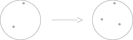
Figure 2.3: The classical moduli space has singularities at $u=0,\infty$;the quantum moduli space at $u=\pm\Lambda^{2},\infty$.

But the $SU(2)$ gauge symmetry is never restored. Instead the effective theory is that of an ${\cal N}=2$ supersymmetric Abelian gauge theory, which must be of the general form

$$S={\rm Im}\int d^{4}x\frac{1}{16\pi}\left[\int d^{2}\theta\frac{\partial^{2}{\cal F}}{\partial\Phi^{2}}W^{\alpha}W_{\alpha}+\int d^{2}\theta d^{2}\bar{\theta}\Phi^{\dagger}\frac{\partial{\cal F}}{\partial\Phi}\right]\ ,$$ (2.63)

where ${\cal F}(\Phi)$ is the holomorphic prepotential, that determines the effective coupling constant $\tau$ as $\tau=\partial^{2}{\cal F}/\partial\Phi^{2}$. What Seiberg and Witten have achieved is to determine ${\cal F}$ exactly in the quantum theory - which includes one-loop corrections and instanton contributions - and thereby determined the complete low energy action of the ${\cal N}=2$ theory.

At $u=\Lambda^{2}$ the effective theory is an ${\cal N}=2$ supersymmetric Abelian gauge theory coupled to a massless monopole (at $u=-\Lambda^{2}$ it is coupled to a massless dyon). And there is a ${\bf Z}_{2}$ symmetry ($u\rightarrow-u$) that relates the theories at these two singularities, originating from the $U(1)_{R}$ symmetry of the classical action. These effective theories are derived by the corresponding prepotential which in turn is determined by the periods of a meromorphic differential on the torus $\Sigma$ given by:

$$y^{2}=(x^{2}-\Lambda^{4})(x-u)\ .$$ (2.64)

If $\alpha$ and $\beta$ are the canonical basis homology cycles of the torus, and

$$\lambda=\frac{1}{\sqrt{2}\pi}\frac{x^{2}dx}{y(x,u)}\$$ (2.65)

is the so-called Seiberg-Witten differential, then the result is as follows: the local coordinate $a(u)$ around $u=\infty$ is:

$$a(u)=\int_{\alpha}\lambda\ ,$$ (2.66)

while the coordinate $a_{D}(u)$ around $u=+\Lambda^{2}$ is determined by:

$$a_{D}(u)=\int_{\beta}\lambda\ .$$ (2.67)

The upshot is that $a(u)$ and $a_{D}(u)$ are given by certain hypergeometric functions (see e.g. [35]), which in turn determine the exact prepotential ${\cal F}(a)$ according to:

$$a_{D}=\frac{\partial}{\partial a}{\cal F}(a)\ .$$ (2.68)

The different low energy effective descriptions are connected by duality transformations. As an example, in going from the description around $u=\infty$ to $u=+\Lambda^{2}$ the effective complex coupling constant $\tau$ is changed by the $SL(2,{\bf Z})$-transformation $\tau\rightarrow-1/\tau$ (the full duality group is actually $SL(2,{\bf Z})$, the same as the modular group of the torus $\Sigma$) .

Why can this analysis be applied to a four-manifold $X$ in the topological theory? The reason is that in the twisted theory one can consider any Riemann metric $g$ on $X$ since correlation functions are independent of the metric. In particular, we can take the family of metrics $g_{t}=t^{2}g$, with $t>0$ and where $g$ is a fixed metric. Note that $t$ large corresponds to large coupling constant.

For $t\rightarrow 0$ we get the Witten approach to Donaldson theory [15]. For $t\rightarrow\infty$, on the other hand, one should expect that only the vacua of ${\bf R}^{4}$ are relevant (because the manifold now looks locally flat). Here, twisting the quantum theory near $u=\pm\Lambda^{2}$ gives a topological quantum field theory which is related to the moduli space of Abelian monopoles. Actually, it is possible to show [33] that for manifolds with $b_{2}^{+}>1$, only contributions coming from $u=\pm\Lambda^{2}$ are important - and that contributions away from these singularities vanish as powers of $t$ for $t\rightarrow\infty$. For $b_{2}^{+}=1$, there is a contribution to the Donaldson invariants from an integral over the $u$-plane, which has been calculated explicitly [33], but we will only consider the case where $b_{2}^{+}>1$, as it is much simpler to analyze.

The Monopole Equations

The theory around the monopole singularity is that of an ${\cal N}=2$ supersymmetric Abelian gauge theory coupled to a massless hypermultiplet and the explicit form of the associated topological Abelian field theory has been found [37] by twisting this theory as described earlier for the case of Donaldson theory.

While in Donaldson theory, one studies solutions to the instanton equations, in the Seiberg-Witten approach one studies what has become known as the Seiberg-Witten monopole equations [5] (see e.g. [38, 32] for a rather mathematical introduction). The main feature is that they involve an Abelian gauge potential $A_{\mu}$ and a set of commuting Weyl spinors $M$ and $\overline{M}$, $\overline{M}$ being the hermitian conjugate of $M$.

Strictly speaking, spinors can only be defined on manifolds which obey certain conditions. (The second Steifel-Whitney class $w_{2}(X)\in H^{2}(X,{\bf Z}_{2})$ should be trivial [27] implying for example that ${\bf C}P^{2}$ does not admit spinors). But here one only needs a so-called Spin^c structure, which can be defined on any oriented four-manifold [38] . But we leave the technical difficulties aside and assume that everything is working fine.

Now, let $X$ be an oriented, closed four-manifold with Riemann metric $g_{\mu\nu}$. We choose Clifford matrices $\Gamma_{\mu}$ on $X$ (that is $\{\Gamma_{\mu},\Gamma_{\nu}\}=2g_{\mu\nu}$) and define $\Gamma_{\mu\nu}=\frac{1}{2}\left[\Gamma_{\mu},\Gamma_{\nu}\right]$. The conventions are such that $\Gamma^{\mu}=e^{\mu}_{\alpha}\gamma^{\alpha}$, with vielbeins $e^{\alpha}_{\mu}$ obeying $g_{\mu\nu}=e^{\alpha}_{\mu}e^{\beta}_{\nu}\delta_{\alpha\beta}$. A hermitian representation of the Dirac matrices in flat ${\bf R^{4}}$ is given by

$$\gamma^{0}=i\left(\begin{array}[]{cc}0&1\\ -1&0\end{array}\right),\;\;\gamma^{k}=\left(\begin{array}[]{cc}0&\sigma^{k}\\ \sigma^{k}&0\end{array}\right)\ ,$$ (2.69)

with $k=1,2,3$. In this representation the chirality matrix takes the diagonal form,

$$\gamma_{5}=i^{2}\gamma^{0}\cdots\gamma^{3}=\left(\begin{array}[]{cc}1&0\\ 0&-1\end{array}\right)\ .$$ (2.70)

The Seiberg-Witten monopole equations are then:

$$F^{+}_{\mu\nu} = -\frac{i}{2}\overline{M}\Gamma_{\mu\nu}M\ ,$$

$$D_{A}M = 0\ ,$$ (2.71)

where $D_{A}$ is the Dirac operator:

$$D_{A}=\Gamma^{\mu}D_{\mu}=\Gamma^{\mu}(\partial_{\mu}+\omega_{\mu}+iA_{\mu})\ ,$$ (2.72)

which is twisted by the spin connection $\omega_{\mu}=\frac{1}{8}\omega_{\mu ij}[\gamma^{i},\gamma^{j}]$ ($i,j=1,\ldots,4$) because we are now working on a general (possibly non-flat) four-manifold. Note that there is a natural action of the gauge group on the space of solutions to the equations in (2.3) by which $M$ is mapped to $e^{i\sigma}M$ and $A_{\mu}$ to $A_{\mu}-\partial_{\mu}\sigma$. This leaves the equations in (2.3) invariant.

As discussed in [37, 39] one can write a completely analogous topological field theory based on these monopole equations (for a number of reviews, see e.g. [40, 41, 42]). Let us use the notation of [39] where the topological action is

$$S_{m}^{(4)}=\delta V_{m}^{(4)}\ ,$$ (2.73)

with ($\alpha,\beta=1,\ldots,4$):

$$V_{m}^{(4)} = \int_{X}d^{4}x\sqrt{g}\left\{\left[\nabla_{\alpha}\psi^{\alpha}+\frac{i}{2}(\overline{N}M-\overline{M}N)\right]\lambda-\chi^{\alpha\beta}(B_{\alpha\beta}-F^{+}_{\alpha\beta}-\frac{i}{2}\overline{M}\Gamma_{\alpha\beta}M)\right.$$ (2.74)

$$\left.-\overline{\mu}(\nu-iD_{A}M)-\overline{(\nu-iD_{A}M)}\mu\right\}\ .$$

The BRST algebra is:

$$\begin{array}[]{ll}\delta A_{\alpha}=\psi_{\alpha}\ ,&\mbox{}\\ \delta\psi_{\alpha}=-\partial_{\alpha}\phi\ ,&\delta M=N\ ,\\ \delta\phi=0\ ,&\delta N=i\phi M\ ,\\ \delta\chi_{\alpha\beta}=B_{\alpha\beta}\ ,&\delta\mu=\nu\ ,\\ \delta B_{\alpha\beta}=0\ ,&\delta\nu=i\phi\mu\ ,\\ \delta\lambda=\eta\ ,&\delta\eta=0\ ,\end{array}$$ (2.75)

and as in the Donaldson theory, $\delta^{2}=0$ only up to a gauge transformation. For instance, $\delta^{2}A_{\alpha}=-\partial_{\alpha}\phi$ which is the variation of $A_{\alpha}$ under an infinitesimal gauge transformation generated by $\phi$. The corresponding ghost number assignments of the fields $(A,\phi,\psi,M,N,\lambda,\eta,\chi,B,\mu,\nu)$ are $U=(0,2,1,0,1,-2,-1,-1,0,-1,0)$ – with $(\lambda,\eta)$ the anti-ghost multiplet and Lagrange multiplier fields $(\chi,B)$ and $(\mu,\nu)$. Using these transformation rules one finds the following expression for the topological action in four dimensions [39]:

$$S_{m}^{(4)} = \int_{X}d^{4}x\sqrt{g}\left\{\left[-\Delta\phi+\overline{M}M\phi-i\overline{N}N\right]\lambda-\left[\nabla_{\alpha}\psi^{\alpha}+\frac{i}{2}(\overline{N}M-\overline{M}N)\right]\eta+2i\phi\overline{\mu}\mu\right.$$ (2.76)

$$-\chi^{\alpha\beta}\left[(\nabla_{\alpha}\psi_{\beta}-\nabla_{\beta}\psi_{\alpha})^{+}+\frac{i}{2}(\overline{M}\Gamma_{\alpha\beta}N+\overline{N}\Gamma_{\alpha\beta}M)\right]$$

$$+\frac{1}{4}(F_{\alpha\beta}^{+}+\frac{i}{2}\overline{M}\Gamma_{\alpha\beta}M)^{2}+\frac{1}{2}\overline{D_{A}M}D_{A}M$$

$$\left.+\overline{(iD_{A}N-\Gamma^{\alpha}\psi_{\alpha}M)}\mu-\overline{\mu}(iD_{A}N-\Gamma^{\alpha}\psi_{\alpha}M)\right\}\ ,$$

where the Lagrange multipliers $B$ and $\nu$ have been eliminated by their equations of motion, that is

$$B_{\alpha\beta} = {1\over 2}(F_{\alpha\beta}^{+}+\frac{i}{2}\overline{M}\Gamma_{\alpha\beta}M)\ ,$$

$$\nu = {1\over 2}iD_{A}M\ ,$$ (2.77)

and the bar indicates hermitian conjugation. In this form, it is clear that the dominant contribution to the functional integral coming from the bosonic part of the action is given by the solutions of the monopole equations (2.3).

While in Donaldson theory we have a moduli space which is characterized by its instanton number, the moduli in question is characterized by a monopole charge.

The Weyl spinor $M$ being charged under $U(1)$, here we must consider a $U(1)$ principle bundle over the four-manifold $X$ with an associated line bundle $L$. Topologically a $U(1)$ bundle is characterized by the first Chern class

$$c_{1}(F)=[F/2\pi]\in H^{2}(X,{\bf Z})\ .$$ (2.78)

Introducing a basis $\Sigma_{i}$ of $H_{2}(X,{\bf Z})$ the monopole charges can then be obtained as the total magnetic flux

$$m_{i}=\int_{\Sigma_{i}}c_{1}\ ,$$ (2.79)

integrated over the surface $\Sigma_{i}$. Often the notation $x=-2c_{1}(L)$ is also used. The moduli space – with fixed monopole number $x$ – of solutions to the monopole equations modulo gauge transformations is denoted by ${\cal M}_{x}$. The dimension of this moduli space can be determined by an index theorem [5] and is

$$d=-\frac{2\chi+3\sigma}{4}+c_{1}(L)^{2}\ ,$$ (2.80)

where again $\chi$ is the Euler characteristic and $\sigma$ is the signature of $X$. It is possible to show that the moduli space is a compact (and oriented) manifold [38]. Indeed, $|M|$ is bounded by the scalar curvature of $X$ – and there are accordingly no square-integrable solutions on flat ${\bf R}^{4}$. The (virtual) dimension of the moduli space vanishes, i.e. $d=0$, exactly when:

$$x^{2}=2\chi+3\sigma\ ,$$ (2.81)

and, because of compactness, the moduli space will then consist of a finite number of points denoted by $P_{i,x}$, $i=1,\ldots t_{x}$.

Seiberg-Witten Invariants

Now, because of orientability, with each such point $P_{i,x}$ one can associate a sign $\epsilon_{i,x}=\pm 1$. For each $x$ for which the virtual dimension is zero, i.e. for which Eq. (2.81) holds, one can define an integer $n_{x}$ as

$$n_{x}=\sum_{i}\epsilon_{i,x}\ .$$ (2.82)

These quantities $n_{x}$ are the celebrated Seiberg-Witten invariants. For $b_{2}^{+}>1$ they constitute a set of diffeomorphism invariants of four-manifolds [38] . Because of a vanishing argument, described later, a given four-manifold will only have a finite number of $x^{\prime}s$ for which $n_{x}\neq 0$. On manifolds for which there are only trivial solutions to the monopole equations, these invariants will of course all vanish.

With these invariants at hand, a number of interesting results can be obtained – some completely new results and some often in a much simpler way than with the Donaldson invariants.

First of all, the partition function of Donaldson-Witten theory can be calculated at strong coupling with the result ( see e.g. [42]):

$$Z=c\sum_{x}\delta(x^{2}-2\chi-3\sigma)\left[n_{x}+i^{\Delta}n_{x}\right]\ ,$$ (2.83)

where $\Delta=(\chi+\sigma)/4$ and the constant $c$ in front can be fixed by requiring agreement with the result at weak coupling [30] and is a topological number:

$$c=2^{1+\frac{1}{4}(7\chi+11\sigma)}\ .$$ (2.84)

The delta function in (2.83) means that only zero-dimensional moduli spaces contribute. The second factor is a contribution coming from two parts: one from the singularity at $u=+\Lambda^{2}$ and one from the one at $u=-\Lambda^{2}$.

If the $u$-plane had more than these two singularities, the result in (2.83) would have been radically different.

Secondly, it is natural to ask how these Seiberg-Witten invariants are related to the Donaldson invariants? In Donaldson theory – at least for simply connected $X$ – there are two important observables, namely an operator $I(\Sigma)$ of ghost number two (where $\Sigma$ is any two-dimensional homology cycle) and an operator of dimension four $W_{0}$.

The generating function for the Donaldson invariants is

$$\langle\exp\left(\sum_{i}\alpha_{i}I(\Sigma_{i})+\lambda W_{0}\right)\rangle\ ,$$ (2.85)

where it is understood that one is summing over instanton numbers. Here $\Sigma_{i}$ is a basis of $H_{2}(X,{\bf Z})$, i.e. $i=1,\ldots,{\rm dim}H_{2}(X,{\bf Z})$, and $\lambda,\alpha_{i}$ are complex numbers.

Using the same notation as in [5], we define $v=\sum_{i}\alpha_{i}[\Sigma_{i}]$; here $[\Sigma_{i}]$ is the element in $H^{2}(X,{\bf Z})$ which is Poincaré dual to $\Sigma_{i}$; $v^{2}=\sum_{i,j}\alpha_{i}\alpha_{j}\Sigma_{i}\cdot\Sigma_{j}$, where $\Sigma_{i}\cdot\Sigma_{j}$ is the intersection number of $\Sigma_{i}$ and $\Sigma_{j}$ . Also we define $v\cdot x=\sum_{i}\alpha_{i}(\Sigma_{i},x)$ for any $x\in H^{2}(X,{\bf Z})$.

For manifolds of simple type, that is one for which the generating function in (2.55) obeys $\partial^{2}\Phi/\partial\lambda^{2}-4\Phi=0$, the following relation has been derived by Witten [5]:

$$\langle\exp\left(\sum_{i}\alpha_{i}I(\Sigma_{i})+\lambda W_{0}\right)\rangle = 2^{1+\frac{1}{4}(7\chi+11\sigma)}\left(\exp\left(\frac{v^{2}}{2}+2\lambda\right)\sum_{x}n_{x}e^{v\cdot x}\right.$$ (2.86)

$$\left.\;\;\;\;\;\;+i^{\Delta}\exp\left(-\frac{v^{2}}{2}-2\lambda\right)\sum_{x}n_{x}e^{-iv\cdot x}\right)\ .$$

For a sketch of the derivation, see [42]. As for the partition function there is one important comment. The first term on the right hand side

$$\exp\left(\frac{v^{2}}{2}+2\lambda\right)\sum_{x}n_{x}e^{v\cdot x}\ ,$$ (2.87)

is the contribution from the $u$-plane singularity at $u=\Lambda^{2}$; the second term on the right hand side

$$\exp\left(-\frac{v^{2}}{2}-2\lambda\right)\sum_{x}n_{x}e^{-iv\cdot x}\ ,$$ (2.88)

comes from the singularity at $u=-\Lambda^{2}$. If the vacuum structure had been different from the one predicted by Seiberg and Witten [2, 3] the resulting relation would have been very different with additional terms from other singularities.

Note that these results depend crucially on the connection to the quantum field theory formulation of Donaldson theory and are not proved rigorously. So there is at least no mathematical proof of the conjectured relation between Donaldson and Seiberg-Witten invariants.

However, the form of (2.86) agrees with a result proved by Kronheimer and Mrowka for manifolds of simple type [43], in which the $n_{x}$ were unknown coefficients.

Witten was able to fix the coefficient $2^{1+\frac{1}{4}(7\chi+11\sigma)}$ by requiring agreement with computations on Kähler manifolds and other manifolds where the Donaldson invariants can be computed explicitly [30]. It has later been shown that the resulting formula agrees with all cases, where the Donaldson invariants are known.

But one does not necessarily need the relation – as conjectured from quantum field theory – between Donaldson and Seiberg-Witten invariants. Indeed, completely independent of this, the task of analyzing the solutions of the monopole equations and the connected Seiberg-Witten invariants is a well-defined mathematical problem, that has been shown to lead to many interesting results in topology. (And this is one reason why they have proven to be so important in the mathematics literature).

As an example, we could mention the celebrated proof of the Thom conjecture for embedded surfaces in ${\bf CP}^{2}$ by Kronheimer and Mrowka [44]. By studying the monopole equations on the four-manifold $X={\bf R}\times{\bf S}^{1}\times\Sigma$, Kronheimer and Mrowka showed that if $\Sigma$ is an oriented two-manifold embedded in ${\bf CP}^{2}$ and representing the same homology class as an algebraic curve of degree $d$, then the genus of $\Sigma$ satisfies: $g\geq(d-1)(d-2)/2$. For further discussion, see [38, 32].

As a further check Witten has been able to compute the invariants exactly on Kähler manifolds, where they are non-vanishing [5].

Vanishing Theorems

Among the most important applications of the Seiberg-Witten equations are the so-called vanishing theorems that follow from (2.3).

From a strictly mathematical point of view, these vanishing theorems can be rigorously derived from (2.3) without the use of physical arguments.

The derivation begins by defining

$$s_{\mu\nu}=F^{+}_{\mu\nu}+\frac{i}{2}\overline{M}\Gamma_{\mu\nu}M\ ,\;\;k^{\alpha}=(D_{A}M)^{\alpha}\ .$$ (2.89)

A solution of the monopole equations obeys of course:

$$\int_{X}d^{4}x\sqrt{g}\left({1\over 2}|s|^{2}+|k|^{2}\right)=0\ .$$ (2.90)

One can rewrite this in an interesting way by using that the square of the Dirac operator is (the Lichnerowicz-Weitzenbock formula):

$$D_{A}^{2} = \Gamma^{\mu}\Gamma^{\nu}D_{\mu}D_{\nu}$$ (2.91)

$$= \left({1\over 2}\left\{\Gamma^{\mu},\Gamma^{\nu}\right\}+{1\over 2}[\Gamma^{\mu},\Gamma^{\nu}]\right)D_{\mu}D_{\nu}$$

$$= D^{\mu}D_{\mu}+\frac{i}{2}\Gamma^{\mu\nu}F_{\mu\nu}-\frac{R}{4}\ ,$$

where $R$ is the scalar curvature, and using one of the Fierz identities (details can be found in [45]):

$$\int_{X}d^{4}x\sqrt{g}\left({1\over 2}|s|^{2}+|k|^{2}\right) = \int_{X}d^{4}x\sqrt{g}\left({1\over 2}|F^{+}|^{2}+g^{\mu\nu}D_{\mu}M\overline{D_{\nu}M}\right.$$ (2.92)

$$\left.+{1\over 2}|M|^{4}+\frac{1}{4}R|M|^{2}\right)\ .$$

An immediate consequence is the following vanishing theorem: if $(A,M)$ is a solution to (2.3) and the scalar curvature of $X$ is positive, $R\geq 0$, then

$$F_{\mu\nu}^{+}=0\ ,\;\;M=0\ ,$$ (2.93)

i.e. the only solutions are from the Abelian instanton equations. This in turn implies [5] that a four-manifold $X$ with $b_{2}^{+}>0$ and non-vanishing Seiberg-Witten invariants, that is $n_{x}\neq 0$ for some $x$, cannot have a metric with positive scalar curvature.

As another application of such vanishing arguments, Witten has shown [5] that the Seiberg-Witten invariants vanish on manifolds which are connected sums $X\#Y$ when $b_{2}^{+}>0$ on both $X$ and $Y$, see fig. 2.2.

The curvature scalar $R$ can be taken positive on such a tube and any solution of the Seiberg-Witten equations can therefore be brought to vanish on it, at least when the tube is taken to be very long. Then one can define a $U(1)$ action on the moduli space of solutions. This is obtained by gauge transforming the solutions on $X$ with a constant gauge transformation that keeps the fields on $Y$ fixed. The fixed points of this action are solutions with $M=0$ on $X$ or $Y$, but for $b_{2}^{+}>0$ one can argue that the only such solutions are the trivial ones. So we have a free action on a set of points and this set must therefore be empty.

In particular it follows that four-dimensional Kähler manifolds cannot be obtained as connected sums, since Witten showed [5] that Kähler manifolds have nontrivial invariants.

As stated previously, for a given four-manifold $X$, there will only be a finite number $x$’s for which the Seiberg-Witten invariants $n_{x}\neq 0$. This is derived from the following vanishing theorem [5]. Throwing away the $|DM|^{2}$-term in (2.92) we have,

$$\int_{X}d^{4}x\sqrt{g}{1\over 2}|F^{+}|^{2}\leq-\int_{X}d^{4}x\sqrt{g}\left({1\over 2}|M|^{4}+\frac{1}{4}R|M|^{2}\right)\ .$$ (2.94)

Combined with the obvious inequality

$$\int_{X}d^{4}x\sqrt{g}\left({1\over 2}|M|^{4}+\frac{1}{4}R|M|^{2}\right)\geq-\frac{1}{32}\int_{X}d^{4}x\sqrt{g}R^{2}\ ,$$ (2.95)

we find

$$\int_{X}d^{4}x\sqrt{g}|F^{+}|^{2}\leq\frac{1}{16}\int_{X}d^{4}x\sqrt{g}R^{2}\ .$$ (2.96)

This shows that $\int_{X}d^{4}x\sqrt{g}|F^{+}|^{2}$ is bounded for a class $x$ with $n_{x}\neq 0$. The same is true for $\int_{X}d^{4}x\sqrt{g}|F^{-}|^{2}$ since we have from (2.80):

$$\frac{1}{4}x^{2}=c_{1}(L)^{2} = \frac{1}{(2\pi)^{2}}\int_{X}d^{4}x\sqrt{g}F^{2}$$ (2.97)

$$= \frac{1}{(2\pi)^{2}}\int_{X}d^{4}x\sqrt{g}\left(|F^{+}|^{2}-|F^{-}|^{2}\right)=\frac{2\chi+3\sigma}{4}\ .$$

One can argue that there are only finitely many line-bundles $L$ for which both $\int_{X}d^{4}x\sqrt{g}|F^{\pm}|^{2}$ are bounded [38] – and hence for every four-manifold $X$, there will only be a finite number of non-trivial invariants $n_{x}$.

A number of similar vanishing theorems can also be derived in the lower-dimensional versions of Seiberg-Witten theory.

2.4 Seiberg-Witten Duality in $D<4$

Having considered the Seiberg-Witten duality applied to topological theories in four dimensions, it becomes natural to ask what happens in lower dimensions? Dimensionally reducing the four-dimensional theory by taking $X=X_{n}\times T^{4-n}$ for $n=2,3$ with the radius of the compact directions going to zero, one obtains dimensionally reduced theories in three and two dimensions which by construction are topological [19].

Such dimensional reductions of Donaldson-Witten theory have been known for a long time [46, 47] (and is briefly reviewed below). As far as topological properties are concerned, the analogous dimensional reductions of the four-dimensional dual theory should provide new Abelian topological theories which are duals of the dimensionally reduced Donaldson-Witten theories.

As in [19] we start by dimensionally reducing the Donaldson-Witten theory in four dimensions with an action given in (2.23). Concretely, we take $X$ to be a product manifold $X=Y\times{\bf S}^{1}$ with signature (++++) and assume that all fields are $x^{0}$-independent. Here $Y$ is a compact and oriented three-manifold. Furthermore, we define $\chi^{i}\equiv\chi^{0i}$ such that $\chi^{ij}=\epsilon^{ijk}\chi_{k}$. This gives the three-dimensional action ($i,j,k=1,2,3$),

$$S^{(3)} = \int_{Y}d^{3}x\sqrt{g}\,{\rm Tr}[\frac{1}{4}F_{ij}F^{ij}+\frac{1}{2}F_{ij}\tilde{F}^{ij}+\frac{1}{2}D_{i}\varphi_{0}D^{i}\varphi_{0}-\frac{1}{2}[\varphi_{0},\phi][\varphi_{0},\lambda]+\frac{1}{2}\phi D_{i}D^{i}\lambda$$ (2.98)

$$-i\eta D_{i}\psi^{i}-i\eta[\varphi_{0},\psi_{0}]+2i\epsilon^{ijk}(D_{i}\psi_{j})\chi_{k}+2i[\varphi_{0},\psi_{i}]\chi^{i}+2i\psi_{0}D_{i}\chi^{i}$$

$$-\frac{i}{2}\lambda[\psi_{0},\psi_{0}]-\frac{i}{2}\lambda[\psi_{i},\psi^{i}]-\frac{i}{2}\phi[\eta,\eta]-\frac{1}{8}[\phi,\lambda]^{2}]\ ,$$

where we defined $A_{0}\equiv\varphi_{0}$ and $\tilde{F}_{ij}=\epsilon_{ijk}F_{0k}=-\epsilon_{ijk}D_{k}\varphi_{0}$.

The reduction to two dimensions is obtained by assuming that the three manifold $X$ is a product manifold of the form $Y=\Sigma\times{\bf S}^{1}$ and $x^{1}$-independence of all fields ($\mu,\nu=2,3$):

$$S^{(2)} = \int_{\Sigma}d^{2}x\sqrt{g}\,{\rm Tr}[\frac{1}{4}F_{\mu\nu}F^{\mu\nu}+\frac{1}{2}D_{\mu}\varphi_{0}D^{\mu}\varphi_{0}+\frac{1}{2}D_{\mu}\varphi_{1}D^{\mu}\varphi_{1}+\frac{1}{2}[\varphi_{1},\varphi_{0}]^{2}$$ (2.99)

$$-\frac{1}{2}[\varphi_{0},\phi][\varphi_{0},\lambda]-\frac{1}{2}[\varphi_{1},\phi][\varphi_{1},\lambda]+\frac{1}{2}\phi D_{\mu}D^{\mu}\lambda-i\eta[\varphi_{0},\psi_{0}]-i\eta[\varphi_{1},\psi_{1}]$$

$$-i\eta D_{\mu}\psi^{\mu}+2i\epsilon^{\mu\nu}(D_{\mu}\psi_{\nu})\chi+2i\epsilon^{\mu\nu}[\varphi_{1},\psi_{\mu}]\chi_{\nu}-2i\epsilon^{\mu\nu}(D_{\mu}\psi_{1})\chi_{\nu}$$

$$+2i[\varphi_{0},\psi_{1}]\chi+2i[\varphi_{0},\psi_{\mu}]\chi^{\mu}+2i\psi_{0}D_{\mu}\chi^{\mu}-2i[\varphi_{1},\psi_{0}]\chi$$

$$-\frac{i}{2}\lambda[\psi_{0},\psi_{0}]-\frac{i}{2}\lambda[\psi_{1},\psi_{1}]$$

$$-\frac{i}{2}\lambda[\psi_{\mu},\psi^{\mu}]-\frac{i}{2}\phi[\eta,\eta]-\frac{1}{8}[\phi,\lambda]^{2}$$

$$+\frac{1}{2}[\varphi_{0},\varphi_{1}]\epsilon^{\mu\nu}F_{\mu\nu}+\epsilon^{\mu\nu}D_{\mu}\varphi_{1}D_{\nu}\varphi_{0}]\ ,$$

where we defined $A_{1}\equiv\varphi_{1}$ and $\chi_{1}\equiv\chi$. Though rather complicated this action can be rewritten in a somewhat simplified form by introducing the complex scalar field $\Phi=\varphi_{0}+i\varphi_{1}$. One can then write the action as:

$$S^{(2)} = \int_{\Sigma}d^{2}x\sqrt{g}\,{\rm Tr}[\frac{1}{4}(F_{\mu\nu}-\frac{1}{2}i\epsilon_{\mu\nu}[\Phi,\Phi^{*}])^{2}+\frac{1}{2}D_{\mu}\Phi D_{\mu}\Phi^{*}$$ (2.100)

$$-\frac{1}{2}[\varphi_{0},\phi][\varphi_{0},\lambda]-\frac{1}{2}[\varphi_{1},\phi][\varphi_{1},\lambda]+\frac{1}{2}\phi D_{\mu}D^{\mu}\lambda-i\eta[\varphi_{0},\psi_{0}]-i\eta[\varphi_{1},\psi_{1}]$$

$$-i\eta D_{\mu}\psi^{\mu}+2i\epsilon^{\mu\nu}(D_{\mu}\psi_{\nu})\chi+2i\epsilon^{\mu\nu}[\varphi_{1},\psi_{\mu}]\chi_{\nu}-2i\epsilon^{\mu\nu}(D_{\mu}\psi_{1})\chi_{\nu}$$

$$+2i[\varphi_{0},\psi_{1}]\chi+2i[\varphi_{0},\psi_{\mu}]\chi_{\mu}-2i\psi_{0}D_{\mu}\chi^{\mu}-2i[\varphi_{1},\psi_{0}]\chi$$

$$-\frac{i}{2}\lambda[\psi_{0},\psi_{0}]-\frac{i}{2}\lambda[\psi_{1},\psi_{1}]$$

$$-\frac{i}{2}\lambda[\psi_{\mu},\psi_{\mu}]-\frac{i}{2}\phi[\eta,\eta]-\frac{1}{8}[\phi,\lambda]^{2}]\ .$$

It is easy to check, that the resulting action is a BRST gauge fixing of the anti–self-duality equation in four dimensions, $F_{\alpha\beta}=-\frac{1}{2}\epsilon_{\alpha\beta\gamma\delta}F^{\gamma\delta}$, reduced to two dimensions:

$$F_{\mu\nu} = \frac{1}{2}i\epsilon_{\mu\nu}\left[\Phi,\Phi^{*}\right]\ ,$$

$$D_{\mu}\Phi = 0\ .$$ (2.101)

These equations have been studied, in the context of Riemann surfaces, by Hitchin [20] (though he mainly concentrated on the case where the gauge group is $SO(3)$, rather than $SU(2)$). The main points following from Hitchin’s analysis are: (1) that the moduli space of solutions modulo gauge transformations is a smooth noncompact manifold ${\cal M}$ of dimension $12(g-1)$, where $g$ is the genus of the Riemann surface; (2) that there is a vanishing theorem related to the solutions of (2.4), similar to the vanishing theorem of Donaldson theory in four dimensions and (3) that it is possible to prove the uniformization theorem: that every compact Riemann surface of genus $g\geq 2$ admits a metric of constant negative curvature. It would be nice if one could give a simple proof of this uniformization theorem by using the two-dimensional version of the Seiberg-Witten equations.

However, it would take us to far astray to go into detail with all this, but the main point is that the moduli space of solutions to (2.4) is an object which has some relevance in the mathematics literature. Also Chapline and Grossman [47] has been considering these equations, thereby indicating a connecting of conformal field theory to Donaldson theory. This seems to indicate a possible physical relevance of these equations, however it is not clear whether their results have any signification relation to the analogous dimensionally reduced monopole equations in two dimensions .

Now we can turn to the analogous dimensional reduction of the dual theory, which is an Abelian gauge theory with action given in (2.76). By taking $X=Y\times{\bf S}^{1}$ as before the dimensionally reduced action becomes:

$$S_{m}^{(3)} = \int_{Y}d^{3}x\sqrt{g}\left\{\left[-\Delta\phi+\overline{M}M\phi-i\overline{N}N\right]\lambda-\left[\nabla_{k}\psi^{k}+\frac{i}{2}(\overline{N}M-\overline{M}N)\right]\eta+2i\phi\overline{\mu}\mu\right.$$

$$-2\chi^{k}\left[-\partial_{k}\psi_{0}+\epsilon_{kij}(\nabla_{i}\psi_{j})-\overline{M}\Gamma_{k}N-\overline{N}\Gamma_{k}M\right]$$

$$+\frac{1}{8}(F_{ij}-\epsilon_{ijk}\partial_{k}\varphi_{0}-\epsilon_{ijk}\overline{M}\Gamma_{k}M)^{2}+\frac{1}{2}\overline{(D_{A}+\varphi_{0})M}(D_{A}+\varphi_{0})M$$

$$+\left.\overline{(i(D_{A}+\varphi_{0})N-(\Gamma^{k}\psi_{k}-i\psi_{0})M)}\mu-\overline{\mu}(i(D_{A}+\varphi_{0})N-(\Gamma^{k}\psi_{k}-i\psi_{0})M)\right\}\ ,$$

where $\chi^{i}\equiv\chi^{0i}$ and $\Gamma^{k}=e^{k}_{\hat{s}}\sigma^{\hat{s}}$, $\hat{s}=1,2,3$, are the Dirac matrices in three dimensions.

Generally, computing Donaldson invariants on $Y\times{\bf S}^{1}$, with the radius of the ${\bf S}^{1}$ going to zero, one would expect to obtain invariants of the three-manifold $Y$.

Using Donaldson-Witten theory, the partition function related to (2.23) on $Y\times{\bf S}^{1}$ computes the so-called Rozansky-Witten invariant of $Y$ [48]. On the Seiberg-Witten side, it has been shown that the partition function of the three-dimensional theory (2.4) gives a Seiberg-Witten version of the so-called Casson invariant [39] (as discussed in [49] this, however, only holds when $b_{1}(Y)>1$). A further discussion of this three-dimensional case, which also discusses a non-Abelian version of the Seiberg-Witten monopoles can be found in [50].

The three-dimensional version of the monopole equations can be obtained from the local minima of the classical part of the action in (2.4). These equations are accordingly:

$$F_{ij}-\epsilon_{ijk}\overline{M}\Gamma_{k}M = 0\ ,$$

$$D_{A}M = 0\ ,$$ (2.103)

$$\varphi_{0} = 0\ ,$$

but of course they could have been derived directly by dimensionally reducing the four-dimensional monopole equations (2.3). In (2.4) the last condition is only necessary if we have a nontrivial solution. Otherwise, it can be replaced by the condition $d\varphi_{0}=0$.

Similarly, making a reduction to two dimensions - with $Y=\Sigma\times{\bf S}^{1}$ - results in the following action:

$$S_{m}^{(2)} = \int_{\Sigma}d^{2}x\sqrt{g}\left\{\left[-\Delta\phi+\overline{M}M\phi-i\overline{N}N\right]\lambda-\left[\nabla_{\mu}\psi^{\mu}+\frac{i}{2}(\overline{N}M-\overline{M}N)\right]\eta+2i\phi\overline{\mu}\mu\right.$$ (2.104)

$$-2\chi^{\mu}\left[-\partial_{\mu}\psi_{0}+\epsilon_{\mu\nu}\partial_{\nu}\psi_{1}-\overline{M}\Gamma_{\mu}N-\overline{N}\Gamma_{\mu}M\right]-2\chi\left[\epsilon_{\mu\nu}(\nabla_{\mu}\psi_{\nu})-\overline{M}\sigma_{1}N-\overline{N}\sigma_{1}M\right]$$

$$+\frac{1}{8}(F_{\mu\nu}-\epsilon_{\mu\nu}\overline{M}\sigma_{1}M)^{2}+\frac{1}{4}\partial_{\mu}\varphi_{0}\partial_{\mu}\varphi_{0}+\frac{1}{4}\partial_{\mu}\varphi_{1}\partial_{\mu}\varphi_{1}+\frac{1}{2}\epsilon_{\mu\nu}\partial_{\mu}\varphi_{1}\partial_{\nu}\varphi_{0}$$

$$+\frac{1}{2}\partial_{\mu}\varphi_{1}\epsilon_{\mu\nu}\overline{M}\Gamma_{\nu}M+\frac{1}{2}\partial_{\mu}\varphi_{0}\overline{M}\Gamma_{\mu}M+\frac{1}{4}(\overline{M}\Gamma_{\mu}M)^{2}$$

$$+\frac{1}{2}\overline{(D_{A}+\varphi_{0}+i\varphi_{1}\sigma_{1})M}(D_{A}+\varphi_{0}+i\varphi_{1}\sigma_{1})M$$

$$+\overline{(i(D_{A}+\varphi_{0}+i\varphi_{1}\sigma_{1})N-(\Gamma^{\mu}\psi_{\mu}-i\psi_{0}+\psi_{1}\sigma_{1})M)}\mu$$

$$\left.-\overline{\mu}(i(D_{A}+\varphi_{0}+i\varphi_{1}\sigma_{1})N-(\Gamma^{\mu}\psi_{\mu}-i\psi_{0}+\psi_{1}\sigma_{1})M)\right\}\ ,$$

here $\Gamma^{\mu}=e^{\mu}_{\hat{\rho}}\sigma^{\hat{\rho}}$, $\hat{\rho}=2,3$, are the corresponding Dirac matrices in two dimensions. This reduction gives rise to a two-dimensional topological theory, as one can check that the resulting two-dimensional action obeys $S_{m}^{(2)}=\delta V_{m}^{(2)}$. Here, $V_{m}^{(2)}$ is the dimensional reduction of $V_{m}^{(4)}$, i.e.

$$V_{m}^{(2)} = \int_{X}d^{2}x\sqrt{g}\left\{\left[\nabla_{\mu}\psi^{\mu}+\frac{i}{2}(\overline{N}M-\overline{M}N)\right]\lambda-2\chi(2H-\frac{1}{2}\epsilon_{\mu\nu}F_{\mu\nu}+\overline{M}\sigma_{1}M)\right.$$ (2.105)

$$-2\chi_{\mu}(2H_{\mu}+\epsilon_{\mu\nu}\partial_{\nu}\varphi_{1}-\partial_{\mu}\varphi_{0}-\overline{M}\Gamma_{\mu}M)$$

$$\left.-\overline{\mu}(\nu-i(D_{A}+\varphi_{0}+i\varphi_{1}\sigma_{1})M)-\overline{(\nu-i(D_{A}+\varphi_{0}+i\varphi_{1}\sigma_{1})M)}\mu\right\}.$$

We have defined $\chi\equiv\chi^{1}$, $H^{\mu}\equiv H^{0\mu}$ and $H\equiv H^{1}$.

Computing Donaldson invariants on $\Sigma\times{\bf S}^{1}$, with the radius of the circle going to zero, one would – as in the three-dimensional case – expect to obtain invariants of the two-manifold $\Sigma$. However, when $\Sigma$ is a compact orientable surface its topology is uniquely characterized by a single integer, the genus $g$, so any non-trivial topological invariant will be a function of $g$ and hence contains at most as much information as the function $f(g)=g$. So (at least a priori) nothing interesting seems to be obtained in this direction.

As for the monopole equations they are either inferred from reducing the three-dimensional monopole equations further to two dimensions, or as the minima of the classical part of the action (2.104), which is:

$$S_{0} = \frac{1}{8}(F_{\mu\nu}-\epsilon_{\mu\nu}\overline{M}\sigma_{1}M)^{2}+\frac{1}{4}(\partial_{\mu}\varphi_{1})^{2}+\frac{1}{2}(\partial_{\mu}\varphi_{0})^{2}+\frac{1}{4}(\overline{M}\Gamma_{\mu}M)^{2}$$ (2.106)

$$+\frac{1}{2}|D_{A}M|^{2}+\frac{1}{2}|\varphi_{0}M|^{2}+\frac{1}{2}|\varphi_{1}\sigma_{1}M|^{2}\ .$$

The two-dimensional variant of the Seiberg-Witten equations are consequently as follows:

$$F_{\mu\nu}-\epsilon_{\mu\nu}\overline{M}\sigma_{1}M = 0\ ,$$

$$D_{A}M = 0\ ,$$

$$\overline{M}\Gamma_{\mu}M = 0\ ,$$

$$\varphi_{0} = 0\ ,$$

$$\varphi_{1} = 0\ .$$ (2.107)

If $(A,M)$ is a trivial solution, then the last two conditions can be replaced by $d\varphi_{0}=d\varphi_{1}=0$.

Though very similar to Hitchin’s self-duality equations these equations of course describe a totally different moduli space: the former is a moduli space of solutions to a $U(1)$-problem while the latter is related to $SU(2)$ ”instantons”. However, as is the case in four dimensions, it should be possible to obtain – in a simple way – result obtained by studying solutions of the Hitchin equations, in terms of the moduli space corresponding to monopole equations as (2.4). To my knowledge, this has not been done in the literature.

However, a number of vanishing theorems, similar to those previously considered in four dimensions can be derived in this context of a two-dimensional surface $\Sigma$ [19, 44]. In fact, it follows from Eq. (2.4), that if $(A,M)$ is a solution of the two-dimensional monopole equations then the pair must obey the following identity [19]

$$\int_{\Sigma}d^{2}x\sqrt{g}(\frac{1}{4}|F|^{2}+\overline{D^{\mu}M}D_{\mu}M+\frac{1}{2}|\overline{M}\sigma_{1}M|^{2}+\frac{1}{4}R|M|^{2})=0\ ,$$ (2.108)

where $R$ is the scalar curvature. If there is a metric so that $R$ is positive on $X$ then this implies that $F_{\mu\nu}=0$ and $M=0$ are the only solutions. On a sphere, for example, we are actually looking at flat Abelian connections. One might therefore naively worry that on a surface of genus $g$ there are only trivial solutions. However, a surface of genus $g\geq 2$ admits a metric of constant negative curvature and the argument does not apply.

Without assuming any positivity of the scalar curvature one can also derive the following inequality:

$$\int_{\Sigma}d^{2}x\sqrt{g}\frac{1}{4}|F|^{2}\leq\frac{1}{32}\int_{\Sigma}d^{2}x\sqrt{g}R^{2}\ .$$ (2.109)

Inserting this in (2.4) on gets an upper bound on $|M|^{4}$ and this implies that the moduli space is compact as in four dimensions.

Another variant of such vanishing arguments shows that if $\Sigma$ is a genus $g$ surface (taken to be of unit area and constant scalar curvature $-4\pi(2g-2)$) then the first Chern number is bounded as [44]:

$$|c_{1}(\Sigma)|=|\frac{1}{2\pi}\int_{\Sigma}F|\leq 2g-2\ .$$ (2.110)

This result (which basically is just (2.109) in another disguise) plays an important role in the proof of the Thom conjecture by Kronheimer and Mrowka [44].

Finally, let us mention that some explicit solutions to the monopole equations on ${\bf R}^{2}$ have been constructed in [51] and the solutions turn out to be vortex configurations. They are singular, as are the analogous solutions, given by Freund [52], in ${\bf R}^{3}$. As noted by Witten in [5], the monopole equations admit no square-integrable solutions on flat ${\bf R}^{n},n\leq 4$.

The Seiberg-Witten equations have been generalized to non-Abelian monopoles, mainly by Labastida and Mariño and is reviewed in [40]. Furthermore, the Donaldson invariants have been computed by, e.g., Moore and Witten on four-manifolds with $b_{2}^{+}=1$ [33] and by Mariño and Moore on non-simply connected manifolds [53]. In the latter case the ”invariants” are not really invariants since they are not constant functions on the space of metrics but only piecewise constant.

The generalization to non-Abelian monopoles is especially interesting since mathematicians are studying these to come up with a mathematical proof of the equivalence of Donaldson-Witten and Seiberg-Witten invariants. The idea being that both the instanton and the Abelian Seiberg-Witten moduli space appear as boundaries of a so-called non-Abelian $PU(2)$-moduli space and that some cobordism argument may then relate the two, see [54].

Chapter 3 T-Duality in String Theory and in Sigma Models

In this chapter we will be focusing on one duality, namely that of $T$-duality (a useful reference is [55]), and we will be analyzing some consequences imposed by this duality in a variety of sigma models (both bosonic, supersymmetric and heterotic models). These consequences can be formulated as a certain relation between $T$-duality and the renormalization group flow (operator $R$) of such models, namely that they commute: $[T,R]=0$.

We will start by describing $T$-duality as a perturbative (order by order) symmetry of string theory. Then we consider the restrictions of scale and Weyl invariance for consistent string propagation. Such invariances are not mandatory for general two-dimensional sigma models which we treat in the rest of the chapter but are related to the renormalization group (RG) flow of such models. Accordingly, in the following sections we study the relation between $T$-duality and RG flow – as defined by the beta functions –in bosonic sigma models, and the extend to which our ”hypothetical” relation, $[T,R]=0$, determines the exact RG flow. Then we treat the case of supersymmetric and heterotic sigma models in a simplified setting. In both cases it turns out that duality implies strong constraints on the RG flow.

3.1 Introduction

$T$-duality is one of the most important dualities in string theory. It was first discovered in the context of toroidal compactifications of closed strings as an invariance under the change of compactification radius from $R$ to $\alpha^{\prime}/R$ [56]. Later it was shown that this symmetry appears not only in toroidal compactifications, but in all target space backgrounds with isometries [57, 58].

The main property of string theory that enables a $T$-duality is that, in a space with compact dimensions, strings can wrap around nontrivial loops. At the same time, the momentum of the string must be quantized along these compact directions. $T$-duality is basically a symmetry under interchange of these wrapping and momentum modes.

To set the scene we start with the free string action describing a closed string moving in flat Minkowski spacetime

$$S_{0}=\frac{1}{4\pi\alpha^{\prime}}\int_{\Sigma}d^{2}\sigma[\partial_{a}X^{\mu}\partial^{a}X_{\mu}+{\rm fermions}]\ ,$$ (3.1)

where $T=\frac{1}{2\pi\alpha^{\prime}}$ is the string tension. The parameter $\alpha^{\prime}$ plays the role of Planck’s constant such that quantum mechanical perturbation theory for strings is an expansion in $\alpha^{\prime}$. The classical limit then corresponds to $\alpha^{\prime}$ small. The integration is over the worldsheet $\Sigma$ which we take to be without boundary and orientable - this is the description relevant for closed strings. The local coordinates on this worldsheet are $(\sigma,\tau)$ with $0\leq\sigma\leq 2\pi$ and periodic and with $-\infty<\tau<\infty$. In (3.1), the spacetime coordinates $X^{\mu}(\tau,\sigma)$ describe the embedding of the string in spacetime. The fermion terms depend on which kind of string theory we are considering. For the bosonic string such model dependent terms are absent.

In the case of the superstring, the action contains fermionic degrees of freedom $\psi^{\mu}$ residing on the worldsheet. As we go around the periodic direction, the fermions can either be periodic or anti-periodic thereby giving rise to a total of four different sectors as the left- and right-moving modes are treated independently. The Ramond (R) fermion is periodic, while the Neveu-Schwarz (NS) fermion is anti-periodic. The NS-NS sector contains massless spacetime bosons, namely a graviton ($g_{\mu\nu}$), an antisymmetric tensor ($b_{\mu\nu}$) and a scalar dilaton ($\phi$). The fundamental string is charged under the two-form $b_{\mu\nu}$. The R-R sector also contains bosons, which are antisymmetric tensor fields $C_{p}$. Such fields will not play any role in this chapter, but are relevant for the understanding of non-perturbative string theory as discussed in Chapter 4. For completeness, we should mention that the R-NS and NS-R sectors gives the spacetime fermions.

Two classical symmetries of the action in (3.1) will be important in the following: the action is invariant under diffeomorphisms of the worldsheet, which is just a change in the coordinates $(\sigma,\tau)\rightarrow(\sigma^{\prime},\tau^{\prime})$ and also invariant under local Weyl symmetry by which is meant a scaling of the worldsheet metric according to $h_{ab}\rightarrow e^{2\omega(\sigma,\tau)}h_{ab}$. On a flat worldsheet this is a conformal symmetry in which case it implies that the classical energy-momentum tensor vanishes:

$$T_{ab}=-\frac{2\pi}{\sqrt{h}}\frac{\delta S_{0}}{\delta h^{ab}}=0\ .$$ (3.2)

We have started with a theory of strings moving in 26-dimensional spacetime (ten-dimensional for the superstrings). To make the connection with the real (observed) world, we should consider compactifications of string theory. This means that we take our spacetime to be a product $M^{26-d}\times K^{d}$ where usually $M^{26-d}$ is flat $(26-d)$-dimensional Minkowski space and $K^{d}$ is some compact manifold. The simplest compactification is compactification on a circle, $K^{d}={\bf S}^{1}$. Choosing $X^{25}$ as the coordinate curcumnavigating the circle, we must identify $X^{25}\sim X^{25}+2\pi R$ since the wave function should be single valued. Hence, the center of mass momentum is quantized in units of $1/R$ along this direction: $P^{25}=n/R$. The string can wind around the circle any number of times so that if we go along the compactified dimension the string coordinate $X^{25}$ does not have to come back to itself, rather

$$X^{25}(\tau,\sigma+2\pi)=X^{25}(\tau,\sigma)+2\pi mR\ ,\;\;m\in{\bf Z}\ .$$ (3.3)

The two integers $(n,m)$ are called momentum and winding modes respectively and are conserved charges.

Let us analyze what the appearance of these modes implies for the mode expansion of the fields $X^{\mu}$. The equation of motion following from the action (3.1) is a wave equation that implies that the fields can be written as a sum of a left and a right-moving part:

$$X^{\mu}=X^{\mu}_{L}(\tau+\sigma)+X^{\mu}_{R}(\tau-\sigma)$$ (3.4)

and the periodicity of the $\sigma$-coordinate implies that the mode expansions are

$$X^{\mu}_{L} = x^{\mu}_{L}+\alpha^{\prime}p^{\mu}_{L}(\tau+\sigma)+i\sqrt{\alpha^{\prime}}\sum_{n\neq 0}\frac{1}{n}\alpha^{\mu}_{n}e^{-in(\tau+\sigma)}\ ,$$

$$X^{\mu}_{R} = x^{\mu}_{R}+\alpha^{\prime}p^{\mu}_{R}(\tau-\sigma)+i\sqrt{\alpha^{\prime}}\sum_{n\neq 0}\frac{1}{n}\tilde{\alpha}^{\mu}_{n}e^{-in(\tau-\sigma)}\ ,$$ (3.5)

where $x^{\mu}_{L}+x^{\mu}_{R}=x^{\mu}_{CM}$ is the center of mass position and $p^{\mu}_{L}+p^{\mu}_{L}=P^{\mu}$ is the total center of mass momentum. With the periodicity conditions (3.3) on the $X^{25}$ coordinate we can then write

$$X^{25}=x^{25}_{CM}+\alpha^{\prime}\frac{n}{R}\tau+mR\sigma+{\rm osc.}$$ (3.6)

It then follows that

$$p_{L}^{25} = \frac{1}{2}\left(\frac{n}{R}+\frac{mR}{\alpha^{\prime}}\right)\ ,$$

$$p_{R}^{25} = \frac{1}{2}\left(\frac{n}{R}-\frac{mR}{\alpha^{\prime}}\right)\ .$$ (3.7)

Now, the spectrum of the string theory is determined by the mass-shell condition [23]:

$$E^{2} = P^{2}+(\frac{n}{R}-\frac{mR}{\alpha^{\prime}})^{2}+\frac{4}{\alpha^{\prime}}N_{L}$$ (3.8)

$$= P^{2}+(\frac{n}{R}+\frac{mR}{\alpha^{\prime}})^{2}+\frac{4}{\alpha^{\prime}}N_{R}\ ,$$

where $P$ is the momentum in the noncompact directions and $N_{L}$ and $N_{R}$ are the oscillator levels of the string.

It follows from (3.8) that the spectrum is invariant under the interchange of momentum and winding modes ($n\leftrightarrow m$), if we change $R$ according to

$$R\rightarrow\alpha^{\prime}/R\ .$$ (3.9)

This symmetry of string theory is called target space duality (or $T$-duality for short). The result in (3.9) means that compactification on a small radius $(R/\sqrt{\alpha^{\prime}}\ll 1)$ is equivalent to compactification on a large radius $(R/\sqrt{\alpha^{\prime}}\gg 1)$. This is of course very interesting and different from the situation in field theory since a particle will have a spectrum which is basically only determined by the momentum in the compact direction - there is no such thing as a winding number!

Also $T$-duality seems to suggest that there is a minimum length scale in string theory: by using one or the other formulation we can restrict to $R\geq\sqrt{\alpha^{\prime}}$.

Another important interpretation of $T$-duality is that it can be seen as a parity transformation on the right-moving coordinates: in terms of the left- and right-moving momentum (3.1), the $T$-duality transformation is simply:

$$p^{25}_{L}\leftrightarrow p^{25}_{L},\;\;\;p^{25}_{R}\leftrightarrow-p^{25}_{R}\ .$$ (3.10)

Without changing the spectrum, one can also change the oscillator modes according to

$$\alpha_{n}^{25}\leftrightarrow\alpha_{n}^{25},\;\;\;\tilde{\alpha}_{n}^{25}\leftrightarrow-\tilde{\alpha}_{n}^{25}\ .$$ (3.11)

This means – because of (3.1) – that $T$-duality can be viewed as the transformation

$$X^{25}=X^{25}_{L}+X^{25}_{R}\;\;\rightarrow X^{\prime 25}=X^{25}_{L}-X^{25}_{R}\ ,$$ (3.12)

which is a spacetime parity transformation that acts only on the right-movers (in the case of superstrings, this would be supplemented with the transformation of the worldsheet fermion $\psi_{R}\rightarrow-\psi_{R}$, in the directions where duality is performed).

So far we have considered free string theory. However, the $T$-duality transformation also acts nontrivially on the string coupling constant, which is determined by the dilaton as $g=\langle e^{\phi}\rangle$. The transformation can be determined by noting that the 25-dimensional coupling constant $g_{25}$ is related to the 26-dimensional coupling by

$$g^{2}=2\pi Rg_{25}^{2}\ ,$$ (3.13)

and must be invariant under duality (since the $T$-duality only acts in the 26’th direction), so

$$g^{2}\rightarrow g^{\prime 2}=\frac{2\pi\alpha^{\prime}}{R}g^{2}_{25}\ .$$ (3.14)

In conclusion $T$-duality must act as

$$R\rightarrow R^{\prime}=\alpha^{\prime}/R\ ,\;\;g\rightarrow g^{\prime}=\frac{g\sqrt{\alpha^{\prime}}}{R}\ .$$ (3.15)

These transformations were first derived by Buscher [57] by requiring duality to be a symmetry of the full string theory with interactions. Moreover, since the coupling constant is basically unchanged, this duality transformation maps the weak coupling limit of one theory to the weak coupling limit of another theory. As an example, it is seen that this procedure yields a duality between Type IIA string theory compactified on a circle of radius $R$ and Type IIB theory compactified on a circle of radius $\alpha^{\prime}/R$ [59, 60].

The description relevant for strings moving in a more general background than a flat Minkowski spacetime can be obtained given a nontrivial vacuum expectation value for the massless NS-NS bosons $g_{\mu\nu},b_{\mu\nu}$ and $\phi$. These can be incorporated by using the vertex operators of the massless fields [23]. This gives the following generalization of (3.1) as the worldsheet action describing a string moving in a curved background:

$$S=\frac{1}{4\pi\alpha^{\prime}}\int_{\Sigma}d^{2}\sigma\sqrt{h}\,\left[h^{ab}g_{\mu\nu}(X)+\frac{i\epsilon^{ab}}{\sqrt{h}}b_{\mu\nu}(X)\right]\partial_{a}X^{\mu}\partial_{b}X^{\nu}+\frac{1}{4\pi}\int_{\Sigma}d^{2}\sigma\sqrt{h}\,R^{(2)}\phi(X)\ .$$ (3.16)

Here $h_{ab}$ is the worldsheet metric, $g_{\mu\nu}(X)$ is the background metric, $b_{\mu\nu}(X)$ is the antisymmetric tensor and $\phi(X)$ is the dilaton field. $R^{(2)}$ is the worldsheet Ricci scalar, so the last term is only relevant on a curved worldsheet. $X^{\mu}(\sigma)$ gives a map $\Sigma\rightarrow M$ from the worldsheet into the target space $M$ and can conveniently be thought of as defining local coordinates on $M$. $M$ is then some Riemann manifold with metric tensor $g_{\mu\nu}$.

Historically, an action of the form (3.16) arise in the context of what is called a non-linear sigma model. In contrast to the Minkowski space action (3.1), this action (3.16) is no longer quadratic in $X^{\mu}$ and accordingly it describes an interacting two-dimensional field theory.

However, not every such background – as defined by $g_{\mu\nu}$, $b_{\mu\nu}$ and $\phi$ – yields a consistent string theory. The values of these background fields are restricted by demanding local scale invariance or conformal invariance.

Scale and Weyl Invariance

Let us start by considering invariance under global scale transformations. Classically (3.1) and (3.16) are invariant under scale transformations. This is not necessarily true in the corresponding quantum theory as is seen by considering the scale transformation of the flat worldsheet metric:

$$\delta_{\epsilon}h_{ab}=\epsilon h_{ab}\ .$$ (3.17)

The resulting change in the partition function is

$$-\frac{\epsilon}{2\pi}\int d^{2}\sigma\langle T^{a}_{\ a}(\sigma)\rangle\ ,$$ (3.18)

where $T^{ab}$ is the energy-momentum tensor. Scale invariance therefore requires $T^{a}_{\ a}=\partial_{a}{\cal O}^{a}$, for ${\cal O}^{a}$ some local operators. In classical field theory scale invariance is insured if the coupling constants are dimensionless (the Lagrangian contains no dimensionfull parameters). However divergences in the quantum theory gives rise to a non-vanishing renormalization group (RG) beta function with the consequence that the effective coupling depends on the length scale. For the sigma models in question, the relevant beta functions (or actually beta functionals) are

$$\beta^{g}_{\mu\nu}\equiv\Lambda\frac{d}{d\Lambda}g_{\mu\nu}\ ,\;\beta^{b}_{\mu\nu}\equiv\Lambda\frac{d}{d\Lambda}b_{\mu\nu}\ ,\;\beta^{\phi}\equiv\Lambda\frac{d}{d\Lambda}\phi\ ,$$ (3.19)

where $\Lambda$ is the appropriate renormalization scale parameter. Note that Eq. (3.19) describe a change in geometry.

The renormalization properties of the non-linear sigma model in (3.16) has been studied extensively in the literature, see e.g. [61, 62].

In string theory, scale invariance alone does not ensure consistency. For this also Weyl invariance is required. Classically, the two first terms in (3.16) are also invariant under Weyl rescalings of the worldsheet metric, while the last term breaks it explicitly. Consider now a Weyl transformation of the worldsheet metric

$$\delta_{\omega}h_{ab}=2\omega(\sigma)h_{ab}\ .$$ (3.20)

The resulting change in the partition function is

$$-\frac{1}{2\pi}\int d^{2}\sigma\sqrt{h(\sigma)}\omega(\sigma)\langle T^{a}_{\ a}(\sigma)\rangle\ .$$ (3.21)

So Weyl invariance requires $T^{a}_{\ a}=0$, which evidently is a stronger condition than scale invariance. In the classical theory, given by (3.1), this trace is identically zero. Indeed, this follows from the fact that the classical energy momentum tensor vanishes (3.2). In the quantum theory $T^{a}_{\ a}$ does not vanish and it implies that there is an anomaly in the local worldsheet symmetry. This is the so-called Weyl anomaly. The propagation of the string is only consistent if this anomaly vanishes (in the light-cone gauge it can for example be shown that the theory is only Lorentz invariant if the anomaly is vanishing [63]).

As a side remark we note that $T^{a}_{\ a}$ ought to vanish on a flat worldsheet where we have conformal invariance. This determines

$$T^{a}_{\ a}=a_{1}R^{(2)}\ ,$$ (3.22)

where $a_{1}$ is a constant and $R^{(2)}$ is the Ricci scalar of the worldsheet. The computation of $a_{1}$ is straightforward and the result is [64]:

$$a_{1}=-\frac{c}{12}\ ,$$ (3.23)

where $c$ is the total central charge of the worldsheet conformal field theory. So Weyl invariance is the same as demanding that the total central charge $c$ is zero. This in turn determines the dimension of flat spacetime: the bosonic string propagates in $D=26$ dimensions and the superstring in $D=10$ dimensions.

The sigma model in (3.16) is - as indicated above - not conformally invariant for all backgrounds. The necessary conditions on the background can be calculated using dimensional regularization in $2+\epsilon$ dimensions and calculating those terms of the action that violate the symmetry at the quantum level in the limit $\epsilon\rightarrow 0$. The possible values of the couplings are then determined by requiring the vanishing of these terms. In terms of the so-called Weyl anomaly coefficients $\bar{\beta}^{g}_{\mu\nu}$, $\bar{\beta}^{b}_{\mu\nu}$ and $\bar{\beta}^{\phi}$ one finds [65]:

$$T^{a}_{\ a}=-\frac{1}{2\alpha^{\prime}}(\bar{\beta}^{g}_{\mu\nu}\partial_{a}X^{\mu}\partial^{a}X^{\nu}+\bar{\beta}^{b}_{\mu\nu}\frac{\epsilon^{ab}}{\sqrt{h}}\partial_{a}X^{\mu}\partial_{b}X^{\nu}+\alpha^{\prime}\bar{\beta}^{\phi}R^{(2)})\ .$$ (3.24)

The Weyl anomaly coefficients can obtained using the weak coupling expansion of the sigma model i.e., as a perturbative expansion in $\alpha^{\prime}$ . To first order in $\alpha^{\prime}$ these equations have the following form [66, 67]:

$$\bar{\beta}^{g}_{\mu\nu} = \alpha^{\prime}R_{\mu\nu}+2\alpha^{\prime}\nabla_{\mu}\partial_{\nu}\phi-\frac{\alpha^{\prime}}{4}H_{\mu\lambda\rho}H_{\nu}^{\ \lambda\rho}\ ,$$ (3.25)

$$\bar{\beta}^{b}_{\mu\nu} = -\frac{\alpha^{\prime}}{2}\nabla^{\rho}H_{\rho\mu\nu}+\alpha^{\prime}\nabla^{\rho}\phi H_{\rho\mu\nu}\ ,$$ (3.26)

$$\bar{\beta}^{\phi} = \frac{D-26}{6}-\frac{\alpha^{\prime}}{2}\nabla^{2}\phi+\alpha^{\prime}\nabla_{\omega}\phi\nabla^{\omega}\phi-\frac{\alpha^{\prime}}{24}H_{\mu\nu\lambda}H^{\mu\nu\lambda}\ ,$$ (3.27)

where $D$ is the spacetime (or target space) dimension and $H$ is the field strength of the $b$-field:

$$H_{\mu\nu\lambda}=3\partial_{[\mu}b_{\nu\lambda]}=\partial_{\mu}b_{\nu\lambda}+\partial_{\nu}b_{\lambda\mu}+\partial_{\lambda}b_{\mu\nu}\ .$$ (3.28)

The Weyl anomaly coefficients differ from the beta functions in (3.19) as follows:

$$\bar{\beta}_{\mu\nu}^{g} = \beta_{\mu\nu}^{g}+2\alpha^{\prime}\nabla_{\mu}\partial_{\nu}\phi\ ,$$ (3.29)

$$\bar{\beta}_{\mu\nu}^{b} = \beta_{\mu\nu}^{b}+\alpha^{\prime}{H_{\mu\nu}}^{\lambda}\partial_{\lambda}\phi\ ,$$ (3.30)

$$\bar{\beta}^{\phi} = \beta^{\phi}+\alpha^{\prime}(\partial_{\mu}\phi)^{2}\ .$$ (3.31)

Comparing the result in (3.23) with (3.24), we see that a background $(g,b,\phi)$ with $\bar{\beta}^{g}_{\mu\nu}=\bar{\beta}^{b}_{\mu\nu}=0$ describes a conformal field theory of central charge $c=6\bar{\beta}^{\phi}$. Hence, from (3.24) we conclude that the requirement of conformal invariance or consistent string propagation is tantamount to the condition that the Weyl anomaly coefficients associated with the background must vanish, i.e.

$$\bar{\beta}_{\mu\nu}^{g}=\bar{\beta}_{\mu\nu}^{b}=\bar{\beta}_{\mu\nu}^{\phi}=0\ .$$ (3.32)

There is, in fact, a simple physical interpretation of this condition. The equation $\bar{\beta}_{\mu\nu}^{g}=0$ looks like an Einstein equation (i.e. $R_{\mu\nu}=0$) with source terms coming from dilaton and antisymmetric tensor fields. Also, the equation $\bar{\beta}_{\mu\nu}^{b}=0$ is similar to the Maxwell equation (i.e. $\nabla F=0$) generalized to the antisymmetric tensor field.

Higher order terms in $\alpha^{\prime}$ gives stringy corrections to these Einstein-like equations. At two-loop there is – as we shall discuss later – a correction term to the metric beta function of the form

$$\frac{\alpha^{\prime}}{2}R_{\mu\alpha\beta\gamma}R_{\nu}^{\ \alpha\beta\gamma}\ ,$$ (3.33)

which gives a correction to the Einstein equations.

In General Relativity, the empty space Einstein equation can be derived as the equation of motion from an action of the form

$$S_{E}\sim\int d^{D}x\sqrt{g}R\ .$$ (3.34)

An obvious question then is whether it is possible to give a physically sensible interpretation of all the equations in (3.32) as equations of motion of an effective low energy action? The answer is affirmative and to lowest order in $\alpha^{\prime}$ that effective action is [23]:

$$S^{\prime}=\frac{1}{2\kappa_{0}^{2}}\int d^{D}x\sqrt{g}e^{-2\phi}\left[\frac{-2(D-26)}{3\alpha^{\prime}}+R-\frac{1}{12}H_{\mu\nu\lambda}H^{\mu\nu\lambda}+4\partial_{\mu}\phi\partial^{\mu}\phi\right]\ ,$$ (3.35)

where $1/\kappa_{0}^{2}$ is the gravitational constant. This is the effective action that is expected to appear after integrating out all the massive modes of the string and as such it is a low energy effective action. The action is written in terms of the so-called string metric $g_{\mu\nu}$ and has a nonstandard normalization of the $R$ term. The action can be written in the standard form (as in Eq. (3.34)) by using instead the Einstein metric $\tilde{g}_{\mu\nu}=e^{-2K\phi}g_{\mu\nu}$, where $K$ is a constant to be determined below. More generally, with two metrics related by a spacetime Weyl transformation as $\tilde{g}_{\mu\nu}=\Omega^{2}(X)g_{\mu\nu}$, the Ricci scalars are related as [69] (p. 446):

$$\tilde{R}=\Omega^{-2}\left(R-2(D-1)\nabla^{2}\ln\Omega-(D-2)(D-1)(\nabla_{\lambda}\ln\Omega)(\nabla^{\lambda}\ln\Omega)\right)\ .$$ (3.36)

For $\Omega=e^{-K\phi}$ this is

$$\tilde{R}=e^{2K\phi}\left(R+2K(D-1)\nabla^{2}\phi-K^{2}(D-2)(D-1)(\nabla\phi)^{2}\right)\ ,$$ (3.37)

so to cancel the unwanted dilaton factor in (3.35) we should take $K=-2/(D-2)$. With this choice one finds the following expression for the effective action in terms of the Einstein metric:

$$S^{\prime}_{E}=\frac{1}{2\kappa_{0}^{2}}\int d^{D}x\sqrt{\tilde{g}}\left[\frac{-2(D-26)}{3\alpha^{\prime}}e^{4\phi/(D-2)}+\tilde{R}-\frac{1}{12}H_{\mu\nu\lambda}H^{\mu\nu\lambda}e^{-8\phi/(D-2)}-\frac{4}{D-2}\partial_{\mu}\phi\partial^{\mu}\phi\right]\ .$$ (3.38)

The vanishing of the Weyl anomaly coefficients (3.32) can then be derived as the equations of motion of the effective action (3.35). Define the Lagrange density ${\cal L}$ as

$$S^{\prime}=\frac{1}{2\kappa_{0}^{2}}\int d^{D}x{\cal L}\ .$$ (3.39)

The Euler-Lagrange equations for the antisymmetric tensor (that is $\frac{\partial{\cal L}}{\partial b_{\mu\nu}}-\nabla^{\omega}\frac{\partial{\cal L}}{\partial(\nabla_{\omega}b_{\mu\nu})}=0$) becomes after using the small calculation,

$$\frac{\partial{\cal L}}{\partial\nabla_{\omega}b_{\mu\nu}}=-\frac{1}{12}\sqrt{g}e^{-2\phi}\frac{\partial H^{2}}{\partial\nabla_{\omega}b_{\mu\nu}}=-\frac{1}{6}\sqrt{g}e^{-2\phi}H^{\lambda\kappa\sigma}\frac{\partial H_{\lambda\kappa\sigma}}{\partial\nabla_{\omega}b_{\mu\nu}}=-\frac{1}{2}\sqrt{g}e^{-2\phi}H_{\omega\mu\nu}\ ,$$ (3.40)

that

$$0=\nabla^{\omega}\left(\sqrt{g}e^{-2\phi}H_{\omega\mu\nu}\right)=\sqrt{g}e^{-2\phi}\left(-2\nabla^{\omega}\phi H_{\omega\mu\nu}+\nabla^{\omega}H_{\omega\mu\nu}\right)\ .$$ (3.41)

This implies the equation $\bar{\beta}^{b}_{\mu\nu}=0$. The variation of the action with respect to $\phi$ is:

$$\delta_{\phi}S^{\prime}=-\frac{1}{2\kappa_{0}^{2}}\int d^{D}x\sqrt{g}e^{-2\phi}\left[\frac{-4(D-26)}{3\alpha^{\prime}}+2R-\frac{1}{6}H_{\mu\nu\lambda}H^{\mu\nu\lambda}+8\partial_{\mu}\phi\partial^{\mu}\phi+8\nabla^{2}\phi\right]\cdot\delta\phi$$ (3.42)

and it implies the following equation of motion for the dilaton:

$$0=\frac{2(D-26)}{3\alpha^{\prime}}-R+\frac{1}{12}H^{2}+4(\nabla\phi)^{2}-4\nabla^{2}\phi\ .$$ (3.43)

The variation with respect to the metric background is more complicated. First we need the following relation:

$$\int d^{D}x\sqrt{g}e^{-2\phi}(\nabla\phi)^{2}=\int d^{D}x\sqrt{g}e^{-2\phi}\left(\nabla^{2}\phi-(\nabla\phi)^{2}\right)\ ,$$ (3.44)

which is obtained by a partial integration and using that the metric is covariantly constant. We then choose to write the action in (3.35) as,

$$S^{\prime} = \frac{1}{2\kappa_{0}^{2}}\int d^{D}xe^{-2\phi}\left[-\sqrt{g}\frac{2(D-26)}{3\alpha^{\prime}}+\sqrt{g}R+4\sqrt{g}g^{\mu\nu}\nabla_{\mu}\nabla_{\nu}\phi-4\sqrt{g}g^{\mu\nu}\nabla_{\mu}\phi\nabla_{\nu}\phi\right.$$ (3.45)

$$\left.-\frac{1}{12}\sqrt{g}g^{\mu\nu}g^{\lambda\kappa}g^{\rho\sigma}H_{\mu\lambda\rho}H_{\nu\kappa\sigma}\right]\ ,$$

in which form the dependence on the metric is explicit. The variation of this expression with respect to the metric is

$$\delta_{g}S^{\prime} = \frac{1}{2\kappa_{0}^{2}}\int d^{D}x\sqrt{g}e^{-2\phi}\left[\left(\frac{2(D-26)}{6\alpha^{\prime}}g_{\mu\nu}+R_{\mu\nu}-{1\over 2}g_{\mu\nu}R-2g_{\mu\nu}\nabla^{2}\phi+4\nabla_{\mu}\nabla_{\nu}\phi\right.\right.$$ (3.46)

$$\left.\left.+2g_{\mu\nu}(\nabla\phi)^{2}-4\nabla_{\mu}\phi\nabla_{\nu}\phi\right)\delta g^{\mu\nu}-\frac{1}{12}\left(-\frac{1}{2}g_{\mu\nu}H^{2}+3H_{\mu}^{\ \kappa\lambda}H_{\nu\kappa\lambda}\right)\delta g^{\mu\nu}\right]\ ,$$

where we have used that

$$\delta(\sqrt{g})=-\frac{1}{2}\sqrt{g}g_{\mu\nu}\delta g^{\mu\nu}\ ,$$ (3.47)

and that

$$\delta(\int d^{D}x\sqrt{g}e^{-2\phi}R)=\int d^{D}x\sqrt{g}e^{-2\phi}(R_{\mu\nu}-\frac{1}{2}g_{\mu\nu}R)\delta g^{\mu\nu}\ .$$ (3.48)

After a partial integration, the equation of motion that follows for the metric is:

$$0 = g_{\mu\nu}\frac{D-26}{3\alpha^{\prime}}+R_{\mu\nu}-\frac{1}{2}g_{\mu\nu}R-2g_{\mu\nu}\nabla^{2}\phi+2\nabla_{\mu}\nabla_{\nu}\phi+2g_{\mu\nu}(\nabla\phi)^{2}$$ (3.49)

$$+\frac{1}{24}g_{\mu\nu}H^{2}-\frac{1}{4}H_{\mu}^{\ \kappa\lambda}H_{\nu\kappa\lambda}\ .$$

This equation together with (3.43) is not immediately related to the vanishing of the Weyl anomaly coefficients. But in fact adding Eq. (3.49) and $-{1\over 2}g_{\mu\nu}$ times Eq. (3.43) gives:

$$0=R_{\mu\nu}-\frac{1}{4}H_{\mu}^{\ \kappa\lambda}H_{\nu\kappa\lambda}+2\nabla_{\mu}\nabla_{\nu}\phi\ ,$$ (3.50)

which is the same as $\bar{\beta}^{g}_{\mu\nu}=0$. Similarly, taking the trace of Eq. (3.49) and adding $(1-D/2)$ times Eq. (3.43) gives

$$0=\frac{2(D-26)}{3\alpha^{\prime}}-2\nabla^{2}\phi-\frac{1}{6}H^{2}+4(\nabla\phi)^{2}\ ,$$ (3.51)

which implies $\bar{\beta}^{\phi}=0$, so that indeed the equations of motion of (3.35) imply that the Weyl anomaly coefficients vanish.

$T$-Duality of Sigma Models

So far we have focused on $T$-duality in string theory and on the sigma model description of string propagation in curved backgrounds. While it is true that consistent string propagation requires conformal invariance on the worldsheet (and hence vanishing of the Weyl anomaly coefficients), this is not a requirement for the existence of a $T$-duality in general. As the set of conformal backgrounds is just a small subset of all possible backgrounds, it seems natural to extend the action of duality to all such backgrounds.

Following this philosophy, we will henceforth be studying the properties of the sigma model (which we first take to be bosonic) away from the conformal point. First we derive the $T$-duality transformations of any bosonic sigma model with a target space isometry and then we study the implications of this duality on the renormalization group flow of the model.

In order to derive the duality transformations – which we will do in a truncated model where $\phi$ is identically zero – relating different sigma model backgrounds, we will assume that the target space has an Abelian isometry which can be represented as a translation in a coordinate $X^{0}$ in the target space. It is then simple to see that we can choose “adapted” coordinates $\{X^{0},X^{i}\}$ such that the background fields are independent of $X^{0}$.

To be more precise, we start by assuming that the action (3.16) is invariant under an isometry in the target space. The corresponding Killing vector is denoted by $k^{\mu}$

$$\delta_{\epsilon}X^{\mu}=\epsilon k^{\mu}\ .$$ (3.52)

A straightforward generalization of this is to have several Killing vectors forming an Abelian or maybe non-Abelian group. We will not discuss that generalization here.

Requiring invariance of the action under the Killing symmetry gives us some conditions on the background fields. The first is that the Lie derivative of the metric with respect to the Killing vector vanishes:

$${\cal L}_{k}g_{\mu\nu}=\nabla_{\mu}k_{\nu}+\nabla_{\nu}k_{\mu}=0\ .$$ (3.53)

Also, there must exist some vector $\omega_{\mu}$ such that

$${\cal L}_{k}b_{\mu\nu}=\partial_{\mu}\omega_{\nu}-\partial_{\nu}\omega_{\mu}\ .$$ (3.54)

In adapted coordinates, the isometry acts in the $X^{0}$-direction as a translation $X^{0}\rightarrow X^{0}+\epsilon$. So $k=k^{\mu}\frac{\partial}{\partial X^{\mu}}=\frac{\partial}{\partial X^{0}}$ and the Lie derivative is then just the derivative with respect to $X^{0}$. It is then obvious that the background metric is independent of $X^{0}$. There would seem to be a problem though since the Lie derivative of the antisymmetric tensor is generally not zero but equal to the exterior derivative of a one-form, but actually there is no problem since the action obviously has a gauge symmetry under which

$$b\rightarrow b+d\lambda$$ (3.55)

with $\lambda$ some one-form. In the gauge where

$${\cal L}_{k}\lambda=-\omega\ ,$$ (3.56)

we find

$${\cal L}_{k}(b+d\lambda)={\cal L}_{k}b+d({\cal L}_{k}\lambda)=d\omega+d(-\omega)=0\ ,$$ (3.57)

so that all background fields are actually independent of $X^{0}$. In the following we will assume that such adapted coordinates have been chosen.

To find the dual model we will gauge the isometry in the target space (3.52) by introducing a gauge field $A_{\mu}$ that transforms as $\delta A_{\mu}=-\partial_{\mu}\epsilon$ [70]. Adding a Lagrange multiplier term forces the gauge field to be a pure gauge. The gauged action is then

$$S_{gauged} = \frac{1}{4\pi\alpha^{\prime}}\int_{\Sigma}(g_{\mu\nu}\delta^{ab}+i\epsilon^{ab}b_{\mu\nu})D_{a}X^{\mu}D_{b}X^{\nu}$$ (3.58)

$$+\frac{i}{4\pi\alpha^{\prime}}\int_{\Sigma}\tilde{X}^{0}(\partial_{a}A_{b}-\partial_{b}A_{a})\epsilon^{ab},$$

where we have defined $D_{a}X^{\mu}=\partial_{a}X^{\mu}+k^{\mu}A_{a}$, and $\tilde{X}^{0}$ acts as a Lagrange multiplier. The dual theory is obtained by integrating the $A$-field

$$A_{a}=-\frac{1}{k^{2}}(k^{\mu}g_{\mu\nu}\partial_{a}X^{\nu}+i{\epsilon_{a}}^{b}\partial_{b}\tilde{X}^{0}+i{\epsilon_{a}}^{b}k^{\mu}b_{\mu\nu}\partial_{b}X^{\nu})\ ,$$ (3.59)

which is inserted back into the action (3.58) and then fixing the gauge with the condition $X^{0}=0$. Subsequently, the following expression for the dual action is obtained:

$$\tilde{S}=\frac{1}{4\pi\alpha^{\prime}}\int_{\Sigma} d^{2}\sigma [\frac{1}{g_{00}}\partial_{a}\tilde{X}^{0}\partial^{a}\tilde{X}^{0}+2\frac{b_{0i}}{g_{00}}\partial_{a}\tilde{X}^{0}\partial^{a}X^{i}+(g_{ij}-\frac{g_{0i}g_{0j}-b_{0i}b_{0j}}{g_{00}})\partial_{a}X^{i}\partial^{a}X^{j}$$ (3.60)

$$+i\epsilon^{ab}(\frac{g_{0i}}{g_{00}}\partial_{a}\tilde{X}^{0}\partial_{b}X^{i}+(b_{ij}-\frac{g_{0i}b_{0j}-b_{0i}g_{0j}}{g_{00}})\partial_{a}X^{i}\partial_{b}X^{j})]\ .$$

So the dual background - which is what we intended to derive - is given by

$$\tilde{g}_{00} = {1\over g_{00}}\ ,\ \tilde{g}_{0i}={b_{0i}\over g_{00}}\ ,\ \tilde{b}_{0i}={g_{0i}\over g_{00}}\ ,$$

$$\tilde{g}_{ij} = g_{ij}-{g_{0i}g_{0j}-b_{0i}b_{0j}\over g_{00}}\ ,$$ (3.61)

$$\tilde{b}_{ij} = b_{ij}-{g_{0i}b_{0j}-b_{0i}g_{0j}\over g_{00}}\ .$$

This expression was first derived by Buscher [57]. There is also a dilaton shift [57]

$$\tilde{\phi}=\phi-\frac{1}{2}\ln g_{00}\ .$$ (3.62)

As is clear from the action (3.16), this is, however, a one-loop effect. Basically, this effect follows from the fact that the $T$-duality acts nontrivially on the coupling constant. Indeed, the string coupling is determined by the expectation value of the dilaton field, since $g=\langle e^{\phi}\rangle$, and it therefore follows from ( 3.15) that

$$\phi^{\prime}=\phi-{1\over 2}\ln(R^{2}/\alpha^{\prime})\ .$$ (3.63)

Duality and Renormalization Group Flow

Having considered the renormalization group flow (as encoded by the beta functions) of bosonic sigma models and the $T$-duality of such models, it remains to connect these two subjects.

More generally, one could enquire as to what restrictions can be imposed by duality in quantum field theory and string theory? An important tool in that direction is that of a moduli space, which typically will parametrize a family of quantum field theories. A point in moduli space is then given by a set of parameters $(\lambda_{1},\lambda_{2},\ldots)$. Consider for example the moduli space of toroidal (${\bf S}^{1}$) compactifications of bosonic string theory. Such a parameter is then the radius $R$ of the compactifying circle. What $T$-duality tells us in this case is that the point $\lambda=R$ in parameter space determines the same (bosonic) string theory as that of $\lambda^{\prime}=1/R$. (or that the moduli space should be modded out by ${\bf Z}_{2}$). So in this respect duality symmetry acts as a transformation in moduli (or parameter) space while leaving the partition function invariant.

Another transformation that also acts naturally on this parameter space, is the one of the renormalization group.

In quantum field theory a central concept is that of regularization and renormalization. After proper renormalization the couplings of the theory will be functions of a renormalization scale $\Lambda$. The flow of the parameters is then determined by the renormalization group (RG). This RG also acts naturally in the parameter space as it determines the change in the renormalized parameters as we change the renormalization scale.

With both the $T$-duality and the RG acting as motions in the parameter space it becomes natural to study the interrelation between the two operators (early related work was done by Lütken [71], in which he studied some constraints on the RG flow from duality in the Ising model and the quantum Hall effect).

The requirement that duality symmetry and the RG be mutually consistent is formulated as follows. In full generality, we will assume that we have a system with a parameter space parametrized by a set of couplings, $g^{i}$. The duality symmetry $T$ (which later actually will mean the usual target space duality) acts on the parameter space according to

$$Tg^{i}\equiv\tilde{g}^{i}=\tilde{g}^{i}(g)\ ,$$ (3.64)

and connects equivalent points in parameter space – as the $R\rightarrow\alpha^{\prime}/R$ symmetry of string theory. The renormalization group flow, on the other hand, is given in terms of a set of beta functions

$$Rg^{i}\equiv\beta^{i}(g)=\Lambda\frac{d}{d\Lambda}g^{i}\ ,$$ (3.65)

where $\Lambda$ is the renormalization scale parameter. More generally, if $F(g)$ is any function on the parameter space then the action of these operations are

$$TF(g) = F(\tilde{g}(g))$$

$$RF(g) = \frac{\delta F(g)}{\delta g^{j}}\cdot\beta^{j}(g)\ .$$ (3.66)

The hypothesis that we will bring forward is that the consistency requirement governing the relation between duality and the RG is expressed by [72]:

$$[T,R]=0\ ,$$ (3.67)

which simply asserts that the duality transformations and the RG flow are mutually commuting operators on the parameter space of the theory. Eq. (3.67) is seen to be equivalent to the following relations between beta functions in the original and the dual theory:

$$\beta^{i}(\tilde{g})=\frac{\delta\tilde{g}^{i}}{\delta g^{j}}\cdot\beta^{j}(g)\ ,$$ (3.68)

or that the beta functions should transform as a contravariant vector under duality. In a quantum field theory with duality, the existence - and the consistency - of the duality symmetry should not depend on the renormalization of the model, so what (3.67) really means is that the duality is a quantum symmetry of the quantum field theory. The relation in (3.67) was first explicitly formulated in [72]. Its consequences, and more generally, the conditions on the RG flow from duality, have been investigated in many different contexts and cases. We will list here a few important contributions: $T$-duality (in the context of a bosonic sigma model at one-loop) was first considered in the seminal paper of Haagensen [73]. This analysis was subsequently extended to two-loop in a bosonic sigma model with purely metric background in [72] and [74]. In the first of these papers, it was shown that $[T,R]=0$ continues to be valid at two-loop; in the second paper it was shown that assuming $[T,R]=0$ determines the form of the two-loop beta function. The heterotic sigma models were considered at one-loop in [75]. After cancellation of anomalies it was found that the consistency conditions are exactly satisfied.

Damgaard and Haagensen [76] studied spin systems with Kramers-Wannier symmetry. In this case the duality group is ${\bf Z}_{2}$ and the restrictions were not strong enough to completely determine the RG flows. However, a similar consistency condition on the beta function $\beta(K)$ implies that there must be a first or higher order phase transition at the self-dual point $K=K^{*}$.

Quantum Hall systems with $SL(2,{\bf Z})$ symmetry were studied by Burgess and Lütken in [77]. Here it was shown that requiring a certain symmetry to be commuting with the RG flow (supplemented with some additional mild assumptions), were enough to completely determine the $c$ function - and in particular the RG beta function.

Ritz [78] considered constraints on the RG flow in ${\cal N}=2$ $SU(2)$ supersymmetric models, which exhibit an $S$-duality. Assuming (supplemented with some additional mild assumptions) that the RG flow commutes with a certain subgroup of $SL(2,{\bf Z})/{\bf Z}_{2}$, the exact non-perturbative beta function could be determined. Happily enough, the result coincides with the Seiberg-Witten solution. Similar work was done by Latorre and Lütken [79], in which they also address the question of RG flow constraints in ${\cal N}=0$ gauge theories.

More recent work by Balog, Forgács, Mohammedi, Palla and Schnittger [80] that gives a proof of $[T,R]=0$ at one-loop (for both Abelian and non-Abelian dualities) from first principles will be described in the last part of this chapter.

3.2 Bosonic Models at One-Loop

In this section we will consider the restrictions on RG flow imposed by duality in bosonic sigma models at one-loop. We will follow [72, 73].

The target space of the sigma model is taken to be $D$-dimensional. After going to adapted coordinates as described in the previous section, the relevant action is

$$S=\frac{1}{4\pi\alpha^{\prime}}\int_{\Sigma} d^{2}\sigma [g_{00}(X)\partial_{a}X^{0}\partial^{a}X^{0}+2g_{0i}(X)\partial_{a}X^{0}\partial^{a}X^{i}+g_{ij}(X)\partial_{a}X^{i}\partial^{a}X^{j}$$ (3.69)

$$+i\epsilon^{ab}(2b_{0i}(X)\partial_{a}X^{0}\partial_{b}X^{i}+b_{ij}\partial_{a}X^{i}\partial_{b}X^{j})]\ ,$$

with all background fields independent of $X^{0}$ and $i,j=1,\ldots,D-1$. The corresponding one-loop duality transformations can be found in (3.1).

For $\Sigma$ a curved worldsheet, we must include another background coupling, namely that of the dilaton $\phi(x)$ [66]. After renormalization this and the other couplings will flow as encoded in the RG beta functions:

$$\beta^{g}_{\mu\nu}\equiv\Lambda\frac{d}{d\Lambda}g_{\mu\nu}\ ,\;\beta^{b}_{\mu\nu}\equiv\Lambda\frac{d}{d\Lambda}b_{\mu\nu}\ ,\;\beta^{\phi}\equiv\Lambda\frac{d}{d\Lambda}\phi\ .$$ (3.70)

In studying the relation between duality and the RG flow we might as well use the Weyl anomaly coefficients which for this model are [67]:

$$\bar{\beta}_{\mu\nu}^{g} = \beta_{\mu\nu}^{g}+2\alpha^{\prime}\nabla_{\mu}\partial_{\nu}\phi\ +\nabla_{(\mu}W_{\nu)}\ ,$$ (3.71)

$$\bar{\beta}_{\mu\nu}^{b} = \beta_{\mu\nu}^{b}+\alpha^{\prime}{H_{\mu\nu}}^{\lambda}\partial_{\lambda}\phi\ +H_{\mu\nu}^{\ \ \lambda}W_{\lambda}+\nabla_{[\mu}L_{\nu]}\ ,$$ (3.72)

$$\bar{\beta}^{\phi} = \beta^{\phi}+\alpha^{\prime}(\partial_{\mu}\phi)^{2}+\nabla^{\mu}\phi W_{\mu}\ .$$ (3.73)

Here $L_{\mu},W_{\mu}$ are target tensors depending on the metric and antisymmetric tensor. Under a target diffeomorphism we have e.g. that the metric beta function change as $\beta^{g}_{\mu\nu}\rightarrow\beta^{g}_{\mu\nu}+\nabla_{(\mu}\xi_{\nu)}$, which reflects the fact that the beta functions are ambiguous. However, quite the opposite is true for the Weyl anomaly coefficients: a target reparametrization is accompanied by $W_{\mu}\rightarrow W_{\mu}-\xi_{\mu}$, and in the end the Weyl anomaly coefficients are invariant [67]. This also implies that for the backgrounds that we consider we can assume that the target tensors $W_{\mu}=L_{\mu}=0$, which we therefore will assume henceforth.

In the notation of the last section, the couplings $g^{i}$ are $g^{i}=\{g_{\mu\nu},b_{\mu\nu},\phi\}$. Since we study the RG flow as generated by the Weyl anomaly coefficients, the action of this flow on any functional $F[g,b,\phi]$ is given by

$$RF[g,b,\phi]=\frac{\delta F}{\delta g_{\mu\nu}}\cdot\bar{\beta}^{g}_{\mu\nu}+\frac{\delta F}{\delta b_{\mu\nu}}\cdot\bar{\beta}^{b}_{\mu\nu}+\frac{\delta F}{\delta\phi}\cdot\bar{\beta}^{\phi}\ ,$$ (3.74)

while the action of the duality operation $T$ is

$$TF[g,b,\phi]=F[\tilde{g},\tilde{b},\tilde{\phi}]\ .$$ (3.75)

In the previous section we postulated that the condition for the mutual consistency of renormalization group flow and duality can be formulated as the requirement that the RG flow and duality operations commute in parameter space:

$$[T,R]=0\ .$$ (3.76)

We will start by assuming that this is true at the one-loop order we are considering and then see to what extend this determines the RG flow. Later we will show – by simplifying the resulting equations – that this condition is in fact satisfied at one-loop.

Now, using the R operation on each side of the ”classical” duality transformations in (3.1), we see that this is equivalent to the following set of consistency conditions:

$$\bar{\beta}^{\tilde{g}}_{00} = -\frac{1}{g_{00}^{2}}\bar{\beta}^{g}_{00}\ ,$$

$$\bar{\beta}^{\tilde{g}}_{0i} = -\frac{1}{g_{00}^{2}}(b_{0i}\bar{\beta}^{g}_{00}-\bar{\beta}^{b}_{0i}g_{00})\ ,$$

$$\bar{\beta}^{\tilde{b}}_{0i} = -\frac{1}{g_{00}^{2}}(g_{0i}\bar{\beta}^{g}_{00}-\bar{\beta}^{b}_{0i}g_{00})\ ,$$ (3.77)

$$\bar{\beta}^{\tilde{g}}_{ij} = \bar{\beta}^{g}_{ij}-\frac{1}{g_{00}}(\bar{\beta}^{g}_{0i}g_{0j}+\bar{\beta}^{g}_{0j}g_{0i}-\bar{\beta}^{b}_{0i}b_{0j}-\bar{\beta}^{b}_{0j}b_{0i})+\frac{1}{g_{00}{{}^{2}}}(g_{0i}g_{0j}-b_{0i}b_{0j})\bar{\beta}^{g}_{00}\ ,$$

$$\bar{\beta}^{\tilde{b}}_{ij} = \bar{\beta}^{b}_{ij}-\frac{1}{g_{00}}(\bar{\beta}^{g}_{0i}b_{0j}+\bar{\beta}^{b}_{0j}g_{0i}-\bar{\beta}^{g}_{0j}b_{0i}-\bar{\beta}^{b}_{0i}g_{0j})+\frac{1}{g_{00}{{}^{2}}}(g_{0i}b_{0j}-b_{0i}g_{0j})\bar{\beta}^{g}_{00}\ ,$$

where on the left hand side we denote by e.g. $\bar{\beta}^{\tilde{g}}_{\mu\nu}$ the Weyl anomaly coefficient computed as a functional of the dual geometry. These relations were first presented in [73]. Here it was shown that the known beta functions satisfy the relations up to a target space diffeomorphism and that they are exactly satisfied for the Weyl anomaly coefficients. If, on the other hand, we start by demanding that the consistency relations should be satisfied, how much can be determined? These conditions are very restrictive and indeed it was shown in [73] that they (essentially) determine the one-loop beta functions – to precisely what extend will be clear later.

A simple argument shows that at loop order $\ell$, the tensor structures $T_{\mu\nu}$ which can appear in the beta functions must scale as $T_{\mu\nu}(\Omega g,\Omega b)=\Omega^{1-\ell}T_{\mu\nu}(g,b)$, with $\Omega$ a constant. This is because the $\ell$ loop counterterm has $\alpha^{\prime\ell}$ as a factor and we can express this as,

$$\beta_{\mu\nu}^{(\ell)}(\frac{1}{\alpha^{\prime}}g)=\alpha^{\prime\ell-1}T_{\mu\nu}(g)\ ,$$ (3.78)

so that a scaling $g\rightarrow\Omega g$ of the metric is the same as scaling $\alpha^{\prime}\rightarrow\Omega^{-1}\alpha^{\prime}$.

This implies that to order ${\cal O}(\alpha^{\prime})$, i.e. $\ell=1$, the only tensors which can possibly appear are

$$\beta_{\mu\nu}^{g} = \alpha^{\prime}\left(A_{1}\,R_{\mu\nu}+A_{2}\,H_{\mu\lambda\rho}H_{\nu}^{\;\lambda\rho}+A_{3}\,g_{\mu\nu}R+A_{4}\,g_{\mu\nu}H_{\alpha\beta\gamma}H^{\alpha\beta\gamma}\right)\ ,$$

$$\beta_{\mu\nu}^{b} = \alpha^{\prime}\left(A_{5}\,\nabla^{\lambda}H_{\mu\nu\lambda}\right)\ ,$$ (3.79)

since these scale as $\Omega^{0}$ under global scalings of the background fields, are generally covariant and have the correct symmetry under $(\mu\leftrightarrow\nu)$. Here, $H$ is the exterior derivative of the $b$-field, $H_{\mu\nu\lambda}=3\partial_{[\mu}b_{\nu\lambda]}$, and the constants $A_{1},\ldots,A_{5}$ can be computed from one-loop Feynman diagrams using dimensional regularization; see for example [65]. It was, however, shown in [73] that requiring $[T,R]=0$ and choosing $A_{1}=1$ uniquely determines $A_{2}=-1/4$, $A_{5}=-1/2$ and $A_{3}=A_{4}=0$. Note that the overall factor of the beta function cannot be determined since the relation $[T,R]=0$ is a linear relation at this order. As was also shown in [73] the transformation of the dilaton under duality, $\tilde{\phi}=\phi-{1\over 2}\ln g_{00}$ can be determined from the consistency conditions (3.2) on $g_{\mu\nu}$ and $b_{\mu\nu}$. This gives the remaining consistency condition for the dilaton beta function,

$$\tilde{\bar{\beta}}^{\phi}=\bar{\beta}^{\phi}-\frac{1}{2g_{00}}\bar{\beta}_{00}\ .$$ (3.80)

From this condition one can determine the dilaton beta function up to a global constant. Hence we see that requiring $[T,R]=0$ at this one-loop order determines all beta functions (but only up to a global factor):

$$\beta^{g}_{\mu\nu} = \alpha^{\prime}R_{\mu\nu}-\frac{\alpha^{\prime}}{4}H_{\mu\lambda\rho}H_{\nu}^{\ \lambda\rho}$$ (3.81)

$$\beta^{b}_{\mu\nu} = -\frac{\alpha^{\prime}}{2}\nabla^{\rho}H_{\rho\mu\nu}$$ (3.82)

$$\beta^{\phi} = C-\frac{\alpha^{\prime}}{2}\nabla^{2}\phi-\frac{\alpha^{\prime}}{24}H_{\mu\nu\lambda}H^{\mu\nu\lambda}\ .$$ (3.83)

A standard procedure for verifying the consistency conditions such as the ones which appear in (3.2) is to decompose the background fields (i.e. the metric and antisymmetric tensor) into a form which singles out the direction ($X^{0}$) in which the duality transformation is performed. This is the Kaluza-Klein reduction where the metric is decomposed as:

$$g_{\mu\nu}=\left(\begin{array}[]{cc}a&av_{i}\\ av_{i}&\bar{g}_{ij}+av_{i}v_{j}\end{array}\right)\ ,$$ (3.84)

such that $g_{00}=a,g_{0i}=av_{i}$ and $g_{ij}=\bar{g}_{ij}+av_{i}v_{j}$. With this procedure the antisymmetric tensor components are $b_{0i}\equiv w_{i}$ and $b_{ij}$. In this representation, the duality transformations take the rather simple form $a\rightarrow 1/a$, $v_{i}\leftrightarrow w_{i}$ and $b_{ij}\rightarrow b_{ij}+w_{i}v_{j}-w_{j}v_{i}$. However, the task of actually verifying the consistency conditions is still very lengthy and the fact that the duality group is just ${\bf Z}_{2}$ is rather obscured by the form of the consistency condition in (3.2).

In [72] it was suggested that one should express these conditions in the tangent frame of the target space where the ${\bf Z}_{2}$ structure is evident. This tangent frame is determined by the local vielbeins, i.e. $e_{\mu}^{\ a}e_{\nu}^{\ b}\delta_{ab}=g_{\mu\nu}$, ($a=\hat{0},\alpha$ with $\alpha=1,\ldots D-1$), and a specific solution corresponding to the decomposition of the metric in (3.84) is:

$$e_{\mu}^{\ a}=\left(\begin{array}[]{cc}e_{0}^{\ \hat{0}}&e_{0}^{\ \alpha}\\ e_{i}^{\ \hat{0}}&e_{i}^{\ \alpha}\end{array}\right)\ =\left(\begin{array}[]{cc}\sqrt{a}&0\\ \sqrt{a}v_{i}&\bar{e}_{i}^{\ \alpha}\end{array}\right)\ ,$$ (3.85)

where the notation is $\bar{e}_{i}^{\ \alpha}\bar{e}_{j}^{\ \beta}\delta_{\alpha\beta}=\bar{g}_{ij}$.

In the tangent frame, the Weyl anomaly coefficients have the components:

$$\bar{\beta}^{g}_{ab}=e_{a}^{\ \mu}e_{b}^{\ \nu}\bar{\beta}^{g}_{\mu\nu},\ \ \bar{\beta}^{b}_{ab}=e_{a}^{\ \mu}e_{b}^{\ \nu}\bar{\beta}^{b}_{\mu\nu}\ ,$$ (3.86)

where $e_{a}^{\ \mu}$ is the inverse vielbein, namely

$$e_{a}^{\ \mu}=\left(\begin{array}[]{cc}e_{\hat{0}}^{\ 0}&e_{\hat{0}}^{\ i}\\ e_{\alpha}^{\ 0}&e_{\alpha}^{\ i}\end{array}\right)\ =\left(\begin{array}[]{cc}1/\sqrt{a}&0\\ -v_{\alpha}&\bar{e}_{\alpha}^{\ i}\end{array}\right)\ .$$ (3.87)

The ${\bf Z}_{2}$ symmetry is now easily seen: one uses (3.2) and express them in the tangent frame through (3.86). We are going to illustrate this with two examples; the $\hat{0}\hat{0}$ and the $\alpha\beta$ components:

$$\bar{\beta}^{\tilde{g}}_{\hat{0}\hat{0}}=\tilde{e}_{\hat{0}}^{\ 0}\ \tilde{e}_{\hat{0}}^{\ 0}\ \bar{\beta}^{\tilde{g}}_{00}=a\ \bar{\beta}^{\tilde{g}}_{00}=-{1\over a}\ \bar{\beta}^{g}_{00}=-e_{\hat{0}}^{\ 0}\ e_{\hat{0}}^{\ 0}\ \bar{\beta}^{g}_{00}=-\bar{\beta}^{g}_{\hat{0}\hat{0}}\ ,$$ (3.88)

and

$$\bar{\beta}^{\tilde{g}}_{\alpha\beta} = \tilde{e}_{\alpha}^{\ 0}\ \tilde{e}_{\beta}^{\ 0}\ \bar{\beta}^{\tilde{g}}_{00}+\tilde{e}_{\alpha}^{\ 0}\ \tilde{e}_{\beta}^{\ i}\ \bar{\beta}^{\tilde{g}}_{0i}+\tilde{e}_{\alpha}^{\ i}\ \tilde{e}_{\beta}^{\ 0}\ \bar{\beta}^{\tilde{g}}_{i0}+\tilde{e}_{\alpha}^{\ i}\ \tilde{e}_{\beta}^{\ j}\ \bar{\beta}^{\tilde{g}}_{ij}$$ (3.89)

$$= \bar{e}_{\alpha}^{\ i}\ \bar{e}_{\beta}^{\ j}\ w_{i}w_{j}\ \bar{\beta}^{\tilde{g}}_{00}-\bar{e}_{\alpha}^{\ j}\ \bar{e}_{\beta}^{\ i}\ w_{j}\ \bar{\beta}^{\tilde{g}}_{0i}-\bar{e}_{\alpha}^{\ i}\ \bar{e}_{\beta}^{\ j}\ w_{j}\ \bar{\beta}^{\tilde{g}}_{i0}+\bar{e}_{\alpha}^{\ i}\ \bar{e}_{\beta}^{\ j}\ \bar{\beta}^{\tilde{g}}_{ij}$$

$$= -\frac{1}{a^{2}}\bar{e}_{\alpha}^{\ i}\ \bar{e}_{\beta}^{\ j}\ w_{i}w_{j}\ \bar{\beta}^{g}_{00}+\frac{1}{a^{2}}\bar{e}_{\alpha}^{\ j}\ \bar{e}_{\beta}^{\ i}\ w_{j}(w_{i}\bar{\beta}^{g}_{00}-\bar{\beta}^{b}_{0i}a)$$

$$+\frac{1}{a^{2}}\bar{e}_{\alpha}^{\ i}\ \bar{e}_{\beta}^{\ j}\ w_{j}(w_{i}\bar{\beta}^{g}_{00}-\bar{\beta}^{b}_{0i}a)+\bar{e}_{\alpha}^{\ i}\ \bar{e}_{\beta}^{\ j}\left(\bar{\beta}^{g}_{ij}\right.$$

$$\left.-\frac{1}{a}(\bar{\beta}^{g}_{0i}av_{j}+\bar{\beta}^{g}_{0j}av_{i}-\bar{\beta}^{b}_{0i}w_{j}-\bar{\beta}^{b}_{0j}w_{i})+\frac{1}{a^{2}}(a^{2}v_{i}v_{j}-w_{i}w_{j})\bar{\beta}^{g}_{00}\right)$$

$$= \bar{e}_{\alpha}^{\ i}\ \bar{e}_{\beta}^{\ j}\ v_{i}v_{j}\ \bar{\beta}^{g}_{00}-\bar{e}_{\alpha}^{\ j}\ \bar{e}_{\beta}^{\ i}\ v_{j}\ \bar{\beta}^{g}_{0i}-\bar{e}_{\alpha}^{\ i}\ \bar{e}_{\beta}^{\ j}\ v_{j}\ \bar{\beta}^{g}_{i0}+\bar{e}_{\alpha}^{\ i}\ \bar{e}_{\beta}^{\ j}\ \bar{\beta}^{g}_{ij}$$

$$= \bar{\beta}^{g}_{\alpha\beta}\ .$$

The complete set of consistency conditions is [72]:

$$\bar{\beta}^{\tilde{g}}_{\hat{0}\hat{0}} = -\bar{\beta}^{g}_{\hat{0}\hat{0}}\ ,$$

$$\bar{\beta}^{\tilde{g}}_{\hat{0}\alpha} = \bar{\beta}^{b}_{\hat{0}\alpha}\ \ ,\ \ \bar{\beta}^{\tilde{b}}_{\hat{0}\alpha}=\bar{\beta}^{g}_{\hat{0}\alpha}\ ,$$

$$\bar{\beta}^{\tilde{g}}_{\alpha\beta} = \bar{\beta}^{g}_{\alpha\beta}\ \ ,\ \ \bar{\beta}^{\tilde{b}}_{\alpha\beta}=\bar{\beta}^{b}_{\alpha\beta}\ .$$ (3.90)

In this form the ${\bf Z}_{2}$ duality covariance is now manifest. An obvious question is why the consistency conditions have such a simple form when formulated in the tangent frame?

The task of verifying the consistency conditions (3.2) in the form (3.2) is now very simple. At this point, one needs to express the geometrical tensors which appear in the beta functions in the tangent frame; this has been done for the Riemann tensor, and contractions thereof, in Appendix A. Let us show by explicit calculations that the consistency condition for the metric: $\bar{\beta}^{\tilde{g}}_{\hat{0}\hat{0}}=-\bar{\beta}^{g}_{\hat{0}\hat{0}}$, is satisfied. Using the expressions in Appendix A we find

$$\bar{\beta}^{g}_{\hat{0}\hat{0}} = e_{\hat{0}}^{\ 0}\ e_{\hat{0}}^{\ 0}\ \bar{\beta}^{g}_{00}$$ (3.91)

$$= \frac{1}{a}\left(\alpha^{\prime}R_{00}-\frac{1}{4}\alpha^{\prime}H_{0\lambda\rho}H_{0}^{\ \lambda\rho}+2\alpha^{\prime}\nabla_{0}\partial_{0}\phi\right)$$

$$= \alpha^{\prime}\left(-\frac{1}{2}\bar{\nabla}_{i}a^{i}-\frac{1}{4}a_{i}a^{i}+\frac{a}{4}F_{ij}F^{ij}-\frac{1}{4a}G_{ij}G^{ij}+a^{i}\partial_{i}\phi\right)\ ,$$

while the dual expression is

$$\bar{\beta}^{\tilde{g}}_{\hat{0}\hat{0}} = \alpha^{\prime}\left(\frac{1}{2}\bar{\nabla}_{i}a^{i}-\frac{1}{4}a_{i}a^{i}+\frac{1}{4a}G_{ij}G^{ij}-\frac{a}{4}F_{ij}F^{ij}-a^{i}\partial_{i}\tilde{\phi}\right)\ ,$$ (3.92)

where we have left the dilaton shift undetermined. It is now clear that this consistency condition is satisfied if and only if the transformation of the dilaton is $\tilde{\phi}=\phi-{1\over 2}\ln a$ as claimed in Eq. (3.62). While we did not gain much here by formulating the consistency condition in the tangent frame, the other condition, $\bar{\beta}^{\tilde{g}}_{\alpha\beta}=\bar{\beta}^{g}_{\alpha\beta}$, proves much easier to verify in the tangent frame; with the help of the expressions in the Appendix A, we find

$$\bar{\beta}^{g}_{\alpha\beta} = \bar{e}_{\alpha}^{\ i}\bar{e}_{\beta}^{\ j}\left[\bar{R}_{ij}-{1\over 2}\bar{\nabla}_{i}a_{j}-\frac{1}{4}a_{i}a_{j}-\frac{a}{2}F_{ik}F_{j}^{\ k}-\frac{1}{4}v_{i}v_{j}G_{kl}G^{kl}-{1\over 2}v_{(i}G_{j)k}G^{kl}v_{l}\right.$$ (3.93)

$$-\frac{1}{4}v_{(i}H_{j)kl}G^{kl}-{1\over 2}(\frac{1}{a}+v_{m}v^{m})G_{i}^{\ k}G_{jk}+{1\over 2}v^{k}v^{m}G_{ik}G_{jm}-{1\over 2}H_{km(i}G_{j)}^{\ k}v^{m}$$

$$\left.-\frac{1}{4}H_{ikm}H_{j}^{\ km}+2\bar{\nabla}_{i}\partial_{j}\phi\right]\ .$$

The dual Weyl coefficient is:

$$\bar{\beta}^{\tilde{g}}_{\alpha\beta} = \bar{e}_{\alpha}^{\ i}\bar{e}_{\beta}^{\ j}\left[\bar{R}_{ij}+{1\over 2}\bar{\nabla}_{i}a_{j}-\frac{1}{4}a_{i}a_{j}-\frac{1}{2a}G_{ik}G_{j}^{\ k}-\frac{1}{4}w_{i}w_{j}F_{kl}F^{kl}-{1\over 2}w_{(i}F_{j)k}F^{kl}w_{l}\right.$$ (3.94)

$$-\frac{1}{4}w_{(i}\tilde{H}_{j)kl}F^{kl}-{1\over 2}(a+w_{m}w^{m})F_{i}^{\ k}F_{jk}+{1\over 2}w^{k}w^{m}F_{ik}F_{jm}-{1\over 2}\tilde{H}_{km(i}F_{j)}^{\ k}w^{m}$$

$$\left.-\frac{1}{4}\tilde{H}_{ikm}\tilde{H}_{j}^{\ km}+2\bar{\nabla}_{i}\partial_{j}\phi-\bar{\nabla}_{i}a_{j}\right]\ ,$$

(note that $a_{i}\rightarrow-a_{i}$ under duality at this order in $\alpha^{\prime}$). Inserting that

$$\tilde{H}_{ijk}=H_{ijk}+G_{ij}v_{k}+w_{j}F_{ik}+G_{jk}v_{i}+w_{k}F_{ji}+G_{ki}v_{j}+w_{i}F_{kj}\ ,$$ (3.95)

and after straightforward but also rather tedious calculations, it is found that the two coefficients match: $\bar{\beta}^{\tilde{g}}_{\alpha\beta}=\bar{\beta}^{g}_{\alpha\beta}$ as promised.

Finally, there is the question whether scale invariant models are mapped to dual models which are also scale invariant. This is however, easily seen since the relation corresponding to (3.2) between the beta functions is [72]:

$$\beta^{\tilde{g}}_{\hat{0}\hat{0}} = -\beta^{g}_{\hat{0}\hat{0}}+\alpha^{\prime}\nabla_{(\hat{0}}\xi_{\hat{0})}\ ,$$

$$\beta^{\tilde{g}}_{\hat{0}\alpha} = \beta^{b}_{\hat{0}\alpha}-\alpha^{\prime}H_{\hat{0}\alpha}^{\ \ \gamma}\xi_{\gamma}\ \ ,\ \ \beta^{\tilde{b}}_{\hat{0}\alpha}=\beta^{g}_{\hat{0}\alpha}-\alpha^{\prime}\nabla_{(\hat{0}}\xi_{\alpha)}\ ,$$

$$\beta^{\tilde{g}}_{\alpha\beta} = \beta^{g}_{\alpha\beta}-\alpha^{\prime}\nabla_{(\alpha}\xi_{\beta)}\ \ ,\ \ \beta^{\tilde{b}}_{\alpha\beta}=\beta^{b}_{\alpha\beta}-\alpha^{\prime}H_{\alpha\beta}^{\ \ \gamma}\xi_{\gamma}\ ,$$ (3.96)

where $\xi_{a}=-{1\over 2}e_{a}^{\ \mu}\partial_{\mu}\ln g_{00}$ generates a target space diffeomorphism, and $(ab)=ab+ba$. So, if the original model has $\beta^{g}_{ab}=\beta^{b}_{ab}=0$ then the same is true in the dual model – after performing a target diffeomorphism generated by $-\xi_{a}$.

So far we have demonstrated that our relation $[T,R]=0$ is satisfied at one-loop order for the bosonic sigma model. However in string theory the natural restriction from duality is that the effective action should be invariant under $T$-duality. It therefore becomes natural to investigate further the relation between these two conditions.

The Effective Action

At any loop order the effective action should be such that the equations of motion are identical to the requirement of vanishing Weyl anomaly coefficients. At one-loop order the effective action is given by

$$S=\alpha^{\prime}\int d^{D}x\sqrt{g}e^{-2\phi}\left[R-\frac{1}{12}H_{\mu\nu\lambda}H^{\mu\nu\lambda}+4\partial_{\mu}\phi\partial^{\mu}\phi\right]\ ,$$ (3.97)

where we have chosen the additive constant in the dilaton beta function to be $C=0$ and we are using string metric with conventions such that $2\kappa_{0}^{2}=1$.

Using the one-loop expressions for the beta functions (3.81) this effective action can be written as

$$S=RV\equiv\frac{\delta V}{\delta g^{i}}\cdot\bar{\beta}^{i}\ ,$$ (3.98)

where $V=2\sqrt{g}\exp(-2\phi)$ – which we will call the measure factor – and where the dot implies a functional integration. Our relation relating the RG flow and duality states that $[T,R]=0$, while the natural requirement from string theory is that the low energy effective action should be invariant under duality (since duality should just be a reformulation of the same theory). However, these two conditions are not equivalent – which is maybe not so strange since in string theory we will not have any RG flow: cancellation of the Weyl anomaly requires that the Weyl anomaly coefficients vanish for a consistent string theory.

First, $[T,R]=0$ obviously does not imply that the low energy action is invariant under duality, since using the above relation we have

$$TS=T(RV)=R(TV)=RV=S\ ,$$ (3.99)

only if the measure factor is duality invariant: $TV=V$. Can we go the other way around, that is, if both the effective action and the measure factor are invariant under duality: $TS=S$ and $TV=V$, can we then conclude that duality and RG commute $[T,R]=0$? Using these two conditions we can only conclude that

$$[T,R]V=T(RV)-R(TV)=TS-RV=0\ ,$$ (3.100)

which of course is not the same as $[T,R]=0$ as an operator equation. This can also be demonstrated by looking at the one-loop Weyl anomaly coefficients. If we use the standard duality transformations at one-loop then it is easy to see that they obey $TV=V$ together with $TS=S$, but if we change the RG flow by multiplying $\bar{\beta}^{b}_{\mu\nu}$ with two, say, then duality and RG flow will no longer commute: $[T,R]\neq 0$.

So, in conclusion, while the natural requirement in string theory is that the low energy effective action is invariant, the natural condition in studying duality of sigma models is that duality and RG flow commute (which must be the same as saying that duality is a quantum symmetry). Furthermore, these conditions are not equivalent: if we are able to find a duality transformation $T$ that keeps the low energy action invariant at some order in $\alpha^{\prime}$, then we cannot be sure that this $T$ will obey $[T,R]=0$. The main reason is that the form of the action in (3.97) does not determine the Weyl anomaly coefficients uniquely: while any term $z^{i}$ obeying $z^{i}\cdot(\delta V/\delta g^{i})=0$ can be added to the beta function without changing the form of the action, but with

$$\bar{\beta}^{i}(\tilde{g})+\tilde{z}^{i}(\tilde{g})=\frac{\delta\tilde{g}^{i}}{\delta g^{j}}\cdot(\bar{\beta}^{j}(g)+z^{j}(g))\ .$$ (3.101)

This is clearly not of the form in Eq. (3.68) and the flow is therefore not covariant under duality.

Scheme (In)dependence

In the discussion we have implicitly been using the assumption that the low energy action is given as $S=(\delta V/\delta g^{i})\cdot\bar{\beta}^{i}$. This form of the action is only valid in a specific scheme and has no invariant meaning (scheme ambiguity is here defined as being equivalent to the possibility of having different field redefinitions). What is invariant, or at least expected to be true in any scheme, is that the variation of the action with respect to a coupling $g^{i}$ is linear in the Weyl anomaly coefficients

$$\frac{\delta S}{\delta g^{i}}=G_{ij}\cdot\bar{\beta}^{j}\ ,$$ (3.102)

with $G_{ij}$ invertible. Then the equations of motion will imply that the Weyl anomaly coefficients vanish (which is one way of defining what the low energy effective action should be). However, even formulated this way, it is clear that $T$-duality invariance of the effective action does not generally imply that the Weyl anomaly coefficients transform covariantly. This is because $G_{ij}$ is by construction such that equations of motion implies vanishing Weyl anomaly coefficients; then one could imagine multiplying one $\bar{\beta}^{i}$ with 2 and $G_{ij}$ with $1/2$ and (3.102) would still be satisfied.

This conclusion, that invariance of the background effective action does not imply $[T,R]=0$ seems to be in conflict with the claims made in [83]. In this paper the bosonic, supersymmetric and heterotic sigma model effective action is studied at two-loop order. A set of ”corrected” duality transformations at this order is then found by requiring $T$-duality invariance of the effective action. We would add that this set of duality transformations is not guaranteed to satisfy $[T,R]=0$, but we have not tried explicitly to verify whether actually $[T,R]$ does vanish or not.

Before turning to the case of purely metric background at two-loop, we would like to make a further comment about scheme independence.

One could enquire as to whether the relation $[T,R]=0$ makes any sense independently of field redefinitions. That is, if we imagine that we have one scheme with duality transformations that keeps the low energy action invariant and satisfying $[T,R]=0$, can we then find the duality transformations in any other scheme such that they preserve the consistency condition and keeps the low energy action invariant?

This is in fact possible. As shown by Haagensen [84] (to order ${\cal O}(\alpha^{\prime 2})$) one can explicitly construct the set of transformations keeping the effective action invariant in any other scheme.

On this background, we turn now to the case of two-loop corrections.

3.3 Bosonic Models at Two-Loop

In this section we show that bosonic sigma models have a two-loop beta function which is of the form $\beta^{(2)}_{\mu\nu}=\lambda R_{\mu\alpha\beta\gamma}{R_{\nu}}^{\alpha\beta\gamma}$ where $\lambda$ is a constant which cannot be determined by the analysis [74]. Furthermore, it turns out that the ”classical” $T$-duality transformations gets modified at this order. This has also been discussed in [85, 86].

It is known [87] that the two-loop beta function is scheme independent using the standard set of subtraction schemes determined by minimal and nonminimal subtractions of the one-loop divergent structure $R_{\mu\nu}$. However, this is only [87] true if we consider purely metric backgrounds, so in order not to complicate the discussion we will concentrate on such backgrounds. That is we take

$$g_{\mu\nu}=\left(\begin{array}[]{cc}a&0\\ 0&\bar{g}_{ij}\end{array}\right)\ ,$$ (3.103)

and $b_{\mu\nu}=0$ which implies that the dual background is torsionless also. Furthermore, we define $a_{i}\equiv\partial_{i}\ln a$ and $q_{ij}\equiv\bar{\nabla}_{i}a_{j}+{1\over 2}a_{i}a_{j}$.

For such a background one-loop $T$-duality transformations amounts to $a\rightarrow 1/a$ while $\bar{g}_{ij}$ is left unchanged. Our relation $[T,R]=0$ is satisfied at one-loop as elaborated upon in the last section – so according to our general philosophy we only need to determine the corrections to $T$ such that this relation is also satisfied at two-loop. The resulting duality transformations have been derived, using geometrical and duality arguments alone (i.e. without using any Feynman diagram calculations), in [74]:

$$\ln\tilde{a} = -\ln a+\lambda\alpha^{\prime}a_{i}a^{i}\ ,$$

$$\tilde{g}_{ij} = g_{ij}=\bar{g}_{ij}\ ,$$

$$\tilde{\phi} = \phi-\frac{1}{2}\ln a+\frac{\lambda}{4}\alpha^{\prime}a_{i}a^{i}\ ,$$ (3.104)

here $\lambda$ is an arbitrary constant which is left undetermined by the consistency conditions. The transformation of the dilaton has been found by requiring that the measure factor is invariant in order to have a duality invariant low energy action also.

This set of corrected duality transformations were first derived by Tseytlin [85], motivated by the fact that the ”classical” (i.e. one-loop) duality transformations did not keep the effective two-loop action invariant (he found $\lambda=1/2$). As a puzzle we should add that in that paper Tseytlin derived another set of duality transformations that keeps the string effective action invariant - with the classical relation $\ln\tilde{a}=-\ln a$ and $g_{ij}$ not invariant - but it turns out that $[T,R]=0$ is not satisfied for these transformations. However, this is of course not in contradiction with our general hypothesis that at any order in $\alpha^{\prime}$ should $T$ be such that it commutes with the RG flow.

Using $[T,R]=0$ on both sides of (3.3) we can as usual derive the consistency conditions which are to be satisfied by the beta functions:

$$\frac{1}{\tilde{a}}\tilde{\bar{\beta}}_{00} = -\frac{1}{a}\bar{\beta}_{00}+2\lambda\alpha^{\prime}\left[a^{i}\partial_{i}\left(\frac{1}{a}\bar{\beta}_{00}\right)-\frac{1}{2}a^{i}a^{j}\bar{\beta}_{ij}\right]\ ,$$

$$\tilde{\bar{\beta}}_{ij} = \bar{\beta}_{ij}\ ,$$

$$\tilde{\bar{\beta}}^{\phi} = \bar{\beta}^{\phi}-\frac{1}{2a}\bar{\beta}_{00}+\frac{\lambda}{2}\alpha^{\prime}\left[a^{i}\partial_{i}\left(\frac{1}{a}\bar{\beta}_{00}\right)-\frac{1}{2}a^{i}a^{j}\bar{\beta}_{ij}\right]\ .$$ (3.105)

Scaling arguments alone determine the maximal set of tensors which can appear as counterterms at this loop order as follows. Using that under $g\rightarrow\Omega g$ (with $\Omega$ a global scaling-constant) the metric beta function must scale as $T_{\mu\nu}(\Omega g)=\Omega^{-1}T_{\mu\nu}(g)$ constrains such possible counterterms to having the form

$$\beta_{\mu\nu}^{(2)} = A_{1}\,\nabla_{\mu}\nabla_{\nu}R+A_{2}\,\nabla^{2}R_{\mu\nu}+A_{3}\,R_{\mu\alpha\nu\beta}R^{\alpha\beta}$$ (3.106)

$$+A_{4}\,R_{\mu\alpha\beta\gamma}{R_{\nu}}^{\alpha\beta\gamma}+A_{5}\,R_{\mu\alpha}{R_{\nu}}^{\alpha}+A_{6}\,R_{\mu\nu}R$$

$$+A_{7}\,g_{\mu\nu}\nabla^{2}R+A_{8}\,g_{\mu\nu}R^{2}+A_{9}\,g_{\mu\nu}R_{\alpha\beta}R^{\alpha\beta}$$

$$+A_{10}\,g_{\mu\nu}R_{\alpha\beta\gamma\delta}R^{\alpha\beta\gamma\delta}\ ,$$

(the total number of possible terms at this order is 18, but only ten of these are linearly independent, which can be shown by using the first and second Bianchi identity – see Appendix B). By using that the one-loop Weyl anomaly coefficient satisfies the one-loop consistency condition, one can prove [74] that the two-loop beta functions in the original and dual backgrounds are related by

$$\tilde{\beta}_{ij}^{(2)}=\beta_{ij}^{(2)}-\frac{1}{4}\lambda a_{(i}\partial_{j)}(a^{k}a_{k})\ .$$ (3.107)

Under the duality transformation – which at this order is just $a\rightarrow 1/a$ – the possible tensor structures can be decomposed into even and odd tensors:

$$\beta_{ij}^{(2)}=E_{ij}+O_{ij}\ ,\;\;\;\tilde{E}_{ij}=E_{ij}\ ,\;\;\;\tilde{O}_{ij}=-O_{ij}\ .$$ (3.108)

Using (3.107) we then arrive at the condition:

$$O_{ij}=\frac{1}{8}\lambda a_{(i}\partial_{j)}(a^{k}a_{k})\ .$$ (3.109)

We have to find the linear combination – if there is any – of the ten tensors in (3.106) which satisfy this relation. First, of course, we need to perform a Kaluza-Klein reduction on these terms, which can be determined by the help of the expressions in Appendix A:

$$(1) :\ \nabla_{i}\nabla_{j}R=\bar{\nabla}_{i}\bar{\nabla}_{j}(\bar{R}-{q_{n}}^{n})\ ,$$

$$(2) :\ \nabla^{2}R_{ij}=(\bar{\nabla}^{2}+\frac{1}{2}a_{k}\bar{\nabla}^{k})(\bar{R}_{ij}-\frac{1}{2}q_{ij})-\frac{1}{4}a_{i}a_{j}{q_{n}}^{n}$$

$$\hskip 51.21495pt-\frac{1}{4}a^{k}a_{(i}\left(\bar{R}_{j)k}-\frac{1}{2}q_{j)k}\right)\ ,$$

$$(3) :\ R_{i\alpha j\beta}R^{\alpha\beta}=\frac{1}{4}q_{ij}{q_{n}}^{n}+\bar{R}_{injm}(\bar{R}^{nm}-\frac{1}{2}q^{nm})\ ,$$

$$(4) :\ R_{i\alpha\beta\gamma}{R_{j}}^{\alpha\beta\gamma}=\frac{1}{2}q_{ik}{q_{j}}^{k}+\bar{R}_{iknm}\bar{R_{j}}^{knm}\ ,$$

$$(5) :\ R_{i\alpha}{R_{j}}^{\alpha}=\bar{R}_{ik}{\bar{R}_{j}}^{\;\,k}-{1\over 2}\bar{R}_{k(i}{q_{j)}}^{k}+{1\over 4}q_{ik}{q_{j}}^{k}\ ,$$

$$(6) :\ R_{ij}R=(\bar{R}_{ij}-{1\over 2}q_{ij})(\bar{R}-{q_{n}}^{n})\ ,$$

$$(7) :\ g_{ij}\nabla^{2}R=\bar{g}_{ij}\left[{1\over 2}a^{k}\partial_{k}(\bar{R}-{q_{m}}^{m})\right.$$

$$\hskip 59.75078pt\left.\phantom{{a\over b}}+\bar{\nabla}^{k}\partial_{k}(\bar{R}-{q_{m}}^{m})\right]\ ,$$

$$(8) :\ g_{ij}R^{2}=\bar{g}_{ij}\left(\bar{R}-{q_{m}}^{m}\right)^{2}\ ,$$

$$(9) :\ g_{ij}R_{\alpha\beta}R^{\alpha\beta}=\bar{g}_{ij}\left[\frac{1}{4}({q_{m}}^{m})^{2}+(\bar{R}_{km}-\frac{1}{2}q_{km})^{2}\right]\ ,$$

$$(10) :\ g_{ij}R_{\alpha\beta\gamma\delta}R^{\alpha\beta\gamma\delta}=\bar{g}_{ij}\left[q_{km}q^{km}+\bar{R}_{k\ell mn}\bar{R}^{k\ell mn}\right]\ .$$

The corresponding odd parts of these tensors are:

$$O_{ij}^{(1)} = -\bar{\nabla}_{i}\bar{\nabla}_{j}\bar{\nabla}_{n}a^{n}\ ,$$

$$O_{ij}^{(2)} = \frac{1}{2}a_{k}\bar{\nabla}^{k}\bar{R}_{ij}-\frac{1}{2}\bar{\nabla}^{2}\bar{\nabla}_{i}a_{j}-\frac{1}{4}a_{i}a_{j}\bar{\nabla}_{k}a^{k}\ ,$$

$$O_{ij}^{(3)} = -\frac{1}{2}\bar{R}_{injm}\bar{\nabla}^{n}a^{m}+\frac{1}{8}a_{n}a^{n}\bar{\nabla}_{i}a_{j}+\frac{1}{8}a_{i}a_{j}\bar{\nabla}_{n}a^{n}\ ,$$

$$O_{ij}^{(4)} = \frac{1}{4}a_{k}a_{(i}\bar{\nabla}_{j)}a^{k}\ ,$$

$$O_{ij}^{(5)} = -{1\over 2}\bar{R}_{k(i}\bar{\nabla}_{j)}a^{k}+\frac{1}{8}a_{k}a_{(i}\bar{\nabla}_{j)}a^{k}\ ,$$ (3.111)

$$O_{ij}^{(6)} = -{1\over 2}\bar{R}\bar{\nabla}_{i}a_{j}-\bar{R}_{ij}\bar{\nabla}_{n}a^{n}+{1\over 4}a_{i}a_{j}\bar{\nabla}_{n}a^{n}$$

$$+{1\over 4}a_{n}a^{n}\bar{\nabla}_{i}a_{j}\ ,$$

$$O_{ij}^{(7)} = \bar{g}_{ij}\left[\frac{1}{2}a^{k}\partial_{k}(\bar{R}-\frac{1}{2}a_{m}a^{m})-\bar{\nabla}^{k}\partial_{k}(\bar{\nabla}_{m}a^{m})\right]\ ,$$

$$O_{ij}^{(8)} = \bar{g}_{ij}\left[-2(\bar{\nabla}^{k}a_{k})\bar{R}+(\bar{\nabla}^{k}a_{k})a^{m}a_{m}\right]\ ,$$

$$O_{ij}^{(9)} = \bar{g}_{ij}\left[\frac{1}{4}(\bar{\nabla}^{k}a_{k})a^{m}a_{m}-(\bar{\nabla}_{k}a_{m})\bar{R}^{km}\right.$$

$$\;\;\;\;\;\left.+\frac{1}{4}(\bar{\nabla}_{k}a_{m})a^{k}a^{m}\right]\ ,$$

$$O_{ij}^{(10)} = \bar{g}_{ij}(\bar{\nabla}_{k}a_{m})a^{k}a^{m}\ .$$

It is seen that the only odd term of the form (3.109) is $O_{ij}^{(4)}$ which originated from $A_{4}R_{\mu\alpha\beta\gamma}R_{\nu}^{\ \alpha\beta\gamma}$. Moreover, it is possible to verify that a term like $O_{ij}^{(4)}$ cannot be obtained as a linear combination of the remaining terms. Hence, in conclusion we have shown that with the requirement of covariance of duality under the RG, the two-loop terms in the beta function must be:

$$\beta^{(2)}_{\mu\nu}=\lambda R_{\mu\alpha\beta\gamma}{R_{\nu}}^{\alpha\beta\gamma}\ .$$ (3.112)

One should, however, keep in mind that the constant in front cannot be determined from this simple background – the correct result is $\lambda=1/2$ [66, 67].

We now know that the $(ij)$ component satisfies its consistency condition. What about the $(00)$ component? As it has been demonstrated in [72] the consistency condition for the $(00)$ component is also exactly satisfied, and we can conclude that $[T,R]=0$ remains true at this two-loop order for the bosonic sigma model.

Furthermore, considering the bosonic sigma model on a flat world sheet it is natural to ask whether scale invariant models at this order are mapped to scale invariant models under duality? By rephrasing the consistency conditions (3.3) for the Weyl anomaly coefficients into conditions for the beta functions, this statement is readily found to hold true also at ${\cal O}(\alpha^{\prime 2})$[72].

3.4 Supersymmetric Sigma Models

Having treated the bosonic sigma models at one- and two-loop it becomes natural to ask to what extend $[T,R]=0$ holds true in the supersymmetric versions, which contrary to the bosonic case describes consistent string theories. We start by describing the relevant sigma models [57, 65].

The ${\cal N}=1,2$ Models

There is a simple procedure to construct supersymmetric sigma models from bosonic ones. Using complex coordinates on the worldsheet, the standard bosonic sigma model (involving only metric and antisymmetric tensor) can be written as

$$S=\frac{1}{2\pi\alpha^{\prime}}\int d^{2}zk_{\mu\nu}(X)\partial_{\bar{z}}X^{\mu}\partial_{z}X^{\nu}\ ,$$ (3.113)

where $k_{\mu\nu}=g_{\mu\nu}+b_{\mu\nu}$. A (1,1) supersymmetric model on the worldsheet is then constructed as follows. To the coordinates $(z,\bar{z})$ we add two anticommuting complex coordinates $\theta$ and $\bar{\theta}$, with

$$\theta^{2}=\bar{\theta}^{2}=\{\theta,\bar{\theta}\}=0\ .$$ (3.114)

Then define the superderivatives according to

$$D_{\theta}=\partial_{\theta}+\theta\partial_{z},\;\;D_{\bar{\theta}}=\partial_{\bar{\theta}}+\bar{\theta}\partial_{\bar{z}}\ .$$ (3.115)

They are seen to satisfy

$$D_{\theta}^{2}=\partial_{z},\;D_{\bar{\theta}}^{2}=\partial_{\bar{z}},\;\{D_{\theta},D_{\bar{\theta}}\}=0\ .$$ (3.116)

It is well-known that a conformal transformation $z\rightarrow z^{\prime}$ is defined by the property that $\partial_{z}=(\partial_{z^{\prime}}/\partial_{z})\partial_{z^{\prime}}$; likewise a superconformal transformation $(z,\theta)\rightarrow(z^{\prime},\theta^{\prime})$ obeys $D_{\theta}=(D_{\theta}\theta^{\prime})D_{\theta^{\prime}}$.

A superconformal invariant action can now be written as a simple generalization of (3.113):

$$S=\frac{1}{2\pi\alpha^{\prime}}\int d^{2}zd^{2}\theta k_{\mu\nu}(X)D_{\bar{\theta}}X^{\mu}D_{\theta}X^{\nu}\ ,$$ (3.117)

where $X^{\mu}$ should be understood as a function of both bosonic and fermionic coordinates: $X^{\mu}=X^{\mu}(z,\bar{z},\theta,\bar{\theta})$. On the worldsheet, $X^{\mu}$ is a scalar superfield (it has no worldsheet indices) and after a Taylor expansion in $\theta$ we can write it as

$$X^{\mu}(z,\bar{z},\theta,\bar{\theta})=X^{\mu}+\theta\psi^{\mu}+\bar{\theta}\tilde{\psi}^{\mu}+\theta\bar{\theta}F^{\mu}\ ,$$ (3.118)

where $X^{\mu}$ is a scalar, $\psi^{\mu}$ and $\tilde{\psi^{\mu}}$ are spinors and $F^{\mu}$ is an auxiliary bosonic field. By using this Taylor expansion and performing the integral over the fermionic coordinates (with $\int d^{2}\theta(\theta\bar{\theta})=1$) one obtains [57]

$$S = \frac{1}{2\pi\alpha^{\prime}}\int d^{2}z\left[k_{\mu\nu}(X)\partial_{\bar{z}}X^{\mu}\partial_{z}X^{\nu}-g_{\mu\nu}(X)(\psi^{\mu}{\cal D}_{\bar{z}}\psi^{\nu}+\tilde{\psi}^{\mu}{\cal D}_{z}\tilde{\psi}^{\nu})\right.$$ (3.119)

$$\hskip 28.45274pt\left.+\frac{1}{2}R_{\mu\nu\lambda\rho}(X)\psi^{\mu}\psi^{\nu}\tilde{\psi}^{\lambda}\tilde{\psi}^{\rho}\right]\ ,$$

where we have defined the expressions,

$${\cal D}_{\bar{z}}\psi^{\nu} = \partial_{\bar{z}}\psi^{\nu}+(\Gamma^{\nu}_{\lambda\rho}(X)+\frac{1}{2}H^{\nu}_{\ \lambda\rho}(X))\partial_{\bar{z}}X^{\lambda}\psi^{\rho}\ ,$$

$${\cal D}_{z}\tilde{\psi}^{\nu} = \partial_{z}\tilde{\psi}^{\nu}+(\Gamma^{\nu}_{\lambda\rho}(X)-\frac{1}{2}H^{\nu}_{\ \lambda\rho}(X))\partial_{z}X^{\lambda}\tilde{\psi}^{\rho}\ .$$ (3.120)

Also, the auxiliary field $F$ has been integrated out.

Clearly, the first term in this action is just that of a standard bosonic sigma model. What about spacetime supersymmetry? For general target manifold $M$ the action (3.117) describes a ${\cal N}=1$ supersymmetric model [65], as it is written in a manifestly supersymmetric notation.

The existence of higher (${\cal N}>1$) supersymmetry in the case of metric and torsion is discussed in [88]. We now turn now to the case of purely metric backgrounds, that is $b_{\mu\nu}=0$.

The condition for ${\cal N}=2$ spacetime supersymmetry has been derived by Zumino [89]: the sigma model has ${\cal N}=2$ spacetime supersymmetry if and only if the target space $M$ is a Kähler manifold (a complex manifold is Kähler if the metric is hermitian, that is $g_{ij}=g_{\bar{i}\bar{j}}=0$, and it is locally of the form $g_{i\bar{j}}=\frac{\partial}{\partial z^{i}}\frac{\partial}{\partial\bar{z}^{\bar{j}}}K(z,\bar{z})$, where $K(z,\bar{z})$ is a function called the Kähler potential). The condition for ${\cal N}=4$ symmetry is that $M$ is hyper-Kähler [90]; however for the rest of this section we will mainly concentrate on the ${\cal N}=1,2$ models.

RG Flow

Restricting to the case of torsionless backgrounds we only have the metric tensor beta function to think about. Let us start with ${\cal N}=2$ models. Such models have a metric beta function which is of the general form

$$\beta^{g}_{i\bar{j}}=a_{1}T^{(1)}_{i\bar{j}}+a_{2}T^{(2)}_{i\bar{j}}+a_{3}T^{(3)}_{i\bar{j}}+\ldots\ ,$$ (3.121)

where $T^{(i)}$ is the $i$-loop counterterm. The form of the possible counterterms is – as in the bosonic case – restricted by scaling arguments, but because of ${\cal N}=2$ supersymmetry there is a further restriction on these terms. By Zumino’s theorem [89] the possible tensor counterterms must be ”Kähler” at any given order (since the unrenormalized metric on target space is $g_{i\bar{j}}+T_{i\bar{j}}$). A Kähler tensor is a second rank tensor $T_{IJ}$ with vanishing unmixed components, $T_{ij}=T_{\bar{i}\bar{j}}$ and mixed components which are locally of the form $T_{i\bar{j}}=\partial_{i}\partial_{\bar{j}}S(z,\bar{z})$.

Using the same scaling arguments as in the last section, at one-loop order the possible counterterms are

$$\beta^{g}_{i\bar{j}}=a_{1}R_{i\bar{j}}+b_{1}g_{i\bar{j}}R\ .$$ (3.122)

However, the term proportional to $b_{1}$ is not a Kähler tensor, as it does not have vanishing torsion, so $b_{1}$ must be identically zero. The Ricci tensor $R_{i\bar{j}}=g^{l\bar{k}}R_{i\bar{j}\bar{k}l}$ is actually a Kähler tensor; it satisfies

$$R_{ij}=R_{\bar{i}\bar{j}}=0,\;\;R_{i\bar{j}}=-\partial_{i}\partial_{\bar{j}}\ln\det g\ ,$$ (3.123)

and qualifies therefore as a one-loop counterterm. It has been shown [61] that the one-loop beta function is unchanged by the inclusion of fermions in the ${\cal N}=2$ model and is therefore the same as for the bosonic sigma model,

$$\beta^{(1)}_{i\bar{j}}=R_{i\bar{j}}\ .$$ (3.124)

At two-loop order the possible counterterms are again restricted by the scaling arguments. This will just give us the same ten counterterms as we had in the bosonic case. We can repeat the analysis of two-loop beta functions that was carried out in the bosonic case. Demanding our basic relation $[T,R]=0$, the only possible counterterm is $R_{\mu\gamma\sigma\lambda}R_{\nu}^{\ \gamma\sigma\lambda}$, or on a complex Kähler manifold

$$\beta^{(2)}_{i\bar{j}}=a_{2}R_{i\bar{k}l\bar{m}}R_{\bar{j}}^{\ \bar{k}l\bar{m}}\ .$$ (3.125)

However, this is not a Kähler tensor and therefore we conclude that $a_{2}\equiv 0$. This result is known from the literature [61]: all ${\cal N}=2$ sigma models have vanishing beta function at two-loop and we therefore have essentially derived this result from the requirement of consistency between RG flow and duality!

What about ${\cal N}=1$ models? At one-loop the ${\cal N}=1$ models have a beta function which is proportional to the Ricci tensor as in the ${\cal N}=0,2$ models [61, 90]. This however follows trivially from the ${\cal N}=2$ result: the only possible counterterms are as in (3.122). Now imagine that $b_{1}\neq 0$. Because of universality this must also be true when restricting the target space to be Kähler. But Kähler geometry implies ${\cal N}=2$ supersymmetry and therefore that $b_{1}=0$, which is a contradiction.

The same argument can be carried out for the two-loop term: at two-loop the only possible counterterm is $R_{\mu\gamma\sigma\lambda}R_{\nu}^{\ \gamma\sigma\lambda}$, but this is not a Kähler tensor when restricting to Kähler target spaces and can consequently not appear as a counterterm in the ${\cal N}=1$ models either.

In conclusion, using scaling arguments together with $[T,R]=0$ we have been able to prove that both ${\cal N}=1,2$ supersymmetric sigma models have a vanishing beta function at two-loop (note that we only considered the torsionless case). It is natural to ask what happens for the ${\cal N}=4$ models. Such models are known to be ultraviolet finite, that is, their beta function is identically zero [91]. Their target spaces are hyper-Kähler manifolds so it readily follows from our analysis that the two-loop term must vanish, as a hyper-Kähler manifold is in particular a Kähler manifold. That also the one-loop term must vanish seems to contradict universality, but of course this is not the case: a hyper-Kähler manifold has vanishing Ricci tensor so there can be no one-loop beta function either.

Therefore, we might ask if we can ”prove” that all higher loop counterterms must vanish for the ${\cal N}=4$ models starting with $[T,R]=0$?

The Heterotic Sigma Models

While the problem here is basically the same as before – namely to see to what extend duality can determine the one-loop beta functions – there is a new ingredient in the appearance of a target gauge field. Everything else being the same, we will concentrate on this related gauge field beta function. The sigma model relevant for the heterotic string theories was described in [92].

The gauge field in question, $A_{\mu}^{\ I}$, is in the adjoint of the gauge group $G$, i.e. $I=1,\ldots,{\rm dim}G$, which for the heterotic string is $G=Spin(32)/{\bf Z}_{2}$ or $E_{8}\times E_{8}$ [93]. The relevant sigma model action is [92, 94]:

$$S = \frac{1}{4\pi\alpha^{\prime}}\int d^{2}\sigma\left[\bigl{(}g_{\mu\nu}+b_{\mu\nu}\bigr{)}\partial_{+}X^{\mu}\partial_{-}X^{\nu}+ig_{\mu\nu}\lambda^{\mu}\bigl{(}\partial_{-}\lambda^{\nu}+\bigl{(}\Gamma^{\nu}_{\rho\sigma}+{1\over 2}{H^{\nu}}_{\rho\sigma}\bigr{)}\partial_{-}X^{\rho}\lambda^{\sigma}\bigr{)}+\right.$$ (3.126)

$$\left.+i\psi^{I}\bigl{(}\partial_{+}\psi^{I}+{{A_{\mu}}^{I}}_{J}\partial_{+}X^{\mu}\psi^{J}\bigr{)}+{1\over 2}{F_{\mu\nu}}_{IJ}\lambda^{\mu}\lambda^{\nu}\psi^{I}\psi^{J}\right]\ ,$$

where

$$H_{\mu\nu\rho}=\partial_{\mu}b_{\nu\rho}+\partial_{\nu}b_{\rho\mu}+\partial_{\rho}b_{\mu\nu}\qquad{\rm and}\qquad F_{\mu\nu}=\partial_{\mu}A_{\nu}-\partial_{\nu}A_{\mu}+[A_{\mu},A_{\nu}]\ .$$ (3.127)

Furthermore, the $\lambda^{\mu}$ are left-handed Majorana-Weyl fermions and the $\psi^{I}$ are right-handed Majorana-Weyl fermions.

We will denote by $\xi$ the Killing vector that generates the Abelian isometry which enables duality transformations. Invariance of the action requires a transformation of the gauge field: $\delta_{\xi}A_{\mu}\equiv{\pounds}_{\xi}A_{\mu}={\cal D}_{\mu}\kappa$, where $\kappa$ is a target gauge parameter [95, 96]. In adapted coordinates (where $\xi^{\mu}\partial_{\mu}\equiv\partial_{0}$) we have [95, 96]

$${\cal D}_{\mu}\kappa\equiv\partial_{\mu}\kappa+[A_{\mu},\kappa]=0\ .$$ (3.128)

The duality transformation of the gauge field is [94, 96],

$$\tilde{A_{0}}_{IJ}=-{1\over g_{00}}\mu_{IJ}\ ,$$ (3.129)

and

$$\tilde{A_{i}}_{IJ}={A_{i}}_{IJ}-{g_{0i}+b_{0i}\over g_{00}}\mu_{IJ}\ ,$$ (3.130)

where we have defined $\mu_{IJ}\equiv(\kappa-\xi^{\alpha}A_{\alpha})_{IJ}=(\kappa-A_{0})_{IJ}$ (the latter in adapted coordinates). The corresponding one-loop duality transformations of the metric, antisymmetric tensor and dilaton fields are as usual (and can in any case be found in (3.1) and (3.62)). To study the relation between the renormalization group flow and the duality we need as usual the beta functions (or better the Weyl anomaly coefficients). For the heterotic sigma model, the Weyl anomaly coefficient is to one-loop order [97, 98]:

$$\bar{\beta}^{A}_{\mu}=\beta^{A}_{\mu}+\alpha^{\prime}{F_{\mu}}^{\lambda}\partial_{\lambda}\phi+{\cal O}(\alpha^{\prime 2})\ .$$ (3.131)

and the beta function is [65, 99]:

$$\beta^{A}_{\mu}={1\over 2}\alpha^{\prime}({\bf D}^{\lambda}F_{\lambda\mu}+{1\over 2}{H_{\mu}}^{\lambda\rho}F_{\lambda\rho})+{\cal O}(\alpha^{\prime 2})\ ,$$ (3.132)

with ${\bf D}^{\lambda}$ the covariant derivative that includes both the gauge and metric connections, that is ${\bf D}^{\lambda}F_{\lambda\mu}=\nabla^{\lambda}F_{\lambda\mu}+[A^{\lambda},F_{\lambda\mu}]$. The Weyl anomaly coefficients for the remaining fields have been presented in (3.25), (3.26) and (3.27). The consistency conditions follows from our basic equation

$$[T,R]=0\ ,$$ (3.133)

or in this case

$${\bar{\beta}}^{\tilde{A}}_{0}={1\over g_{00}}{\bar{\beta}}^{A}_{0}+{1\over g_{00}^{2}}(\kappa-A_{0}){\bar{\beta}}_{00}^{g}\ ,$$ (3.134)

$${\bar{\beta}}^{\tilde{A}}_{i}={\bar{\beta}}^{A}_{i}-{1\over g_{00}}\bigr{(}(\kappa-A_{0})({\bar{\beta}}_{0i}^{g}+{\bar{\beta}}_{0i}^{b})-(g_{0i}+b_{0i}){\bar{\beta}}^{A}_{0}\bigl{)}+{1\over g_{00}^{2}}(g_{0i}+b_{0i})(\kappa-A_{0}){\bar{\beta}}_{00}^{g}\ .$$ (3.135)

Are these equations satisfied by and only by (3.132)? This can of course be checked by brute force. To simplify the discussion we will restrict to a diagonal metric background with no torsion, i.e.

$$g_{\mu\nu}=\pmatrix{a&0\cr 0&\bar{g}_{ij}\cr}\ ,$$ (3.136)

and we take $b_{\mu\nu}=0$. ”Classical” duality transformations will then guarantee that there is no torsion in the dual background either, see Eq. (3.1).

With this background the consistency conditions become simply

$${\bar{\beta}}^{\tilde{A}}_{0}={1\over a}{\bar{\beta}}^{A}_{0}+{1\over a^{2}}(\kappa-A_{0})\,{\bar{\beta}}_{00}^{g}\ ,$$ (3.137)

$${\bar{\beta}}^{\tilde{A}}_{i}={\bar{\beta}}^{A}_{i}\ .$$ (3.138)

Upon inserting the known beta functions, and doing the duality transformations, there is, however, a small surprise since this is actually not the result that one finds. Rather the result is [75]:

$${\bar{\beta}}^{\tilde{A}}_{0}={1\over a}{\bar{\beta}}^{A}_{0}+{1\over a^{2}}(\kappa-A_{0})(-{\bar{\beta}}_{00}^{g})\ ,$$ (3.139)

$${\bar{\beta}}^{\tilde{A}}_{i}={\bar{\beta}}^{A}_{i}\ .$$ (3.140)

For (3.137) to be consistent with (3.139) – or in order for duality to be a quantum symmetry – we need to have:

$$(\kappa-A_{0})\,{\bar{\beta}}_{00}^{g}=0\ .$$ (3.141)

In the case of the most general background what this is saying is that $(\kappa-A_{0})=0.$ What is the origin of such a condition?

The answer to this question is that because of anomalies the theory and its dual will only be equivalent when certain conditions are met. Such anomalies come from chiral fermions which are part of the background fields.

The simplest way to cancel the anomalies is to assume that the spin connection and gauge connection match, i.e. $\omega=A$ [23, 94, 96]. That this is a consistent condition – in the sense of duality – follows from the fact that if $\omega=A$ then also $\tilde{\omega}=\tilde{A}$ in the dual theory [94, 96]. It then follows [94, 96] that $\mu=\Omega$, where we define

$$\Omega_{\mu\nu}\equiv{1\over 2}(\nabla_{\mu}\xi_{\nu}-\nabla_{\nu}\xi_{\mu})\ ,$$ (3.142)

In adapted coordinates $\xi_{\mu}=g_{\mu 0}$ and therefore – since the connection is metric compatible – we have $\Omega=0$. This readily answers our question as to the origin of the condition (3.141):

$$\mu_{IJ}=(\kappa-A_{0})_{IJ}=0\ ,$$ (3.143)

because we demand that anomalies must cancel. What this is telling us is that in order for the consistency condition, as applied to the gauge field, to be satisfied requires the cancellation of anomalies (the logic might seem reversed here since in order to have a well defined renormalization group flow the theory should be free of anomalies; however the attitude we are taking here is that we will see how far the requirement of $[T,R]=0$ can take us).

So far we have shown that the consistency conditions (3.137) are satisfied by the Weyl anomaly coefficients given in (3.131). But what we want is the other way around – do the consistency conditions determine the renormalization group flow?

The gauge beta function is a covariant tensor (a vector) on the space of background fields. Together with the scaling arguments in [100] this determines that to one-loop order it must be of the form

$$\beta^{A}_{\mu}=c_{1}\,\alpha^{\prime}{\bf D}^{\lambda}F_{\lambda\mu}+c_{2}\,\alpha^{\prime}{H_{\mu}}^{\lambda\rho}F_{\lambda\rho}\ ,$$ (3.144)

where $c_{1}$ and $c_{2}$ are constants that can be computed using one-loop Feynman diagrams as in [65, 99]. Here, these constants are determined by the beta function constraint:

$${\beta}^{\tilde{A}}_{i}={\beta}^{A}_{i}+{1\over 2}\alpha^{\prime}{F_{i}}^{k}\partial_{k}\ln a\ ,$$ (3.145)

which follows directly from taking the dual of Eq. (3.131) and using that $\bar{\beta}^{\tilde{A}}_{i}=\bar{\beta}^{A}_{i}$. For torsionless background, however, the last term in (3.144) is absent and we can therefore set $c_{2}=0$. Insertion of (3.144) in (3.145) then gives

$$(c_{1}-{1\over 2}){F_{i}}^{k}\partial_{k}\ln a=0\ ,$$ (3.146)

from which we obtain $c_{1}={1\over 2}$, which agrees with the result in Eq. (3.132). We conclude that we were able to uniquely determine the one-loop gauge field beta function – though in the particular case of vanishing torsion. Considering the case of torsion included [75] shows that also the constant $c_{2}$ can be determined by (3.145). The result is $c_{2}=\frac{1}{4}$, which agrees with (3.132).

Thus, the consistency conditions are verified by, and only by, the correct RG flows of the heterotic sigma model. In other words, classical target space duality symmetry survives as a valid quantum symmetry of the heterotic sigma model.

It is, however, not obvious how one should extend this analysis to higher ($\ell\geq 2$) loop orders, since in this case the beta functions contain Lorentz and gauge variant terms [99].

3.5 Open Questions

In this section we will address a few open questions which arise naturally in connection with the situations analyzed in the preceding part of this chapter. In the last part of this section we will describe how the relation $[T,R]=0$ has been derived at one-loop [80].

Open String

We have been analyzing the relation between renormalization group flow and duality for bosonic, supersymmetric (with ${\cal N}=1,2$) and the heterotic sigma models (which have ${\cal N}=1$). It could be interesting to include the case of open (super)strings. In the open string case, the duality transformations are [101],

$$\tilde{A}_{0}=0\qquad,\qquad\tilde{A}_{i}=A_{i}\ .$$ (3.147)

The consistency conditions associated with these transformations,

$$\bar{\beta}^{\tilde{A}}_{0}=0\qquad{\rm and}\qquad\bar{\beta}^{\tilde{A}}_{i}=\bar{\beta}^{A}_{i}\ ,$$ (3.148)

are the same as for the heterotic string with vanishing anomaly. Naively, scaling arguments would then dictate that the only possible form of the gauge field beta function is that of Eq. (3.144). However, this is not the whole story. The reason is that $T$-duality – as discussed further in the next chapter – interchanges the usual Neumann boundary condition $\partial_{n}X=0$ with the Dirichlet condition $\partial_{\tau}X=0$ in the dualized directions. This implies that the ends of the open string are confined to move on D-branes and the position of this hyperplane $f(X^{\mu})$ becomes a dynamical field which should be included in the RG flow. For further discussion see [101].

It could be interesting to include these boundary fields to study the RG flow of the open string sigma model in the presence of D-branes. In some sense one would then have to require $[T,R]=0$ both in the bulk and on the boundary of the worldsheet surface. Maybe this could be important for finding a non-Abelian version of the Born-Infeld action.

Higher Loop Corrections

Having shown that the two-loop beta functions must vanish for the supersymmetric (${\cal N}=1,2$) models, it is natural to enquire as to what happens for higher loop orders. The three-loop correction to the supersymmetric models is known to vanish [102], while the four-loop correction is non-vanishing and very complicated indeed [102]. To perform such an analysis we need to know how the beta functions differ from the Weyl anomaly coefficients. There is a difference at one-loop but no further terms at two-loop. However, there are new terms appearing at three and higher loops, since in this case one cannot set $L_{\mu}=W_{\mu}=0$ [66].

Another complication is that the number of counterterms restricted by scaling arguments can be large – the maximal number of possible terms presumably grows exponentially with the number of loops. At three-loop the counterterm must scale as $T_{\mu\nu}(\Omega g)=\Omega^{-2}T_{\mu\nu}(g)$ and the tensors can be described – in the case of no torsion – as (i) tensors of the form $\nabla\nabla\nabla\nabla R$ (2 terms), (ii) tensors like $R\nabla\nabla R$ (13 terms), (iii) tensors like $\nabla R\nabla R$ (11 terms), (iv) tensors of the form $RRR$ (16 terms) and finally (v) tensors which are of the form $g_{\mu\nu}\times({\rm contractions}$) (16 terms). These tensors (which have not yet been symmetrized) can be found in a paper by Fulling et al. [103]. So just to verify that the three-loop beta functions must vanish for ${\cal N}=1,2$ models seems very complicated from this point of view!

We will end this chapter by mentioning, that more recently Balog et al. [80] has presented a derivation of (3.67) to one-loop order. Following [80], let us write the worldsheet metric as $h_{ab}=e^{\sigma(z)}\delta_{ab}$. Now let $g$ denote collectively the set of renormalized couplings $(g,b,\phi)$ and $g^{0}$ the bare couplings and let $Z^{R}[g;\sigma]$ denote the renormalized partition function ($Z[g;\sigma]$ is the corresponding bare partition function). The starting point is the Weyl anomaly coefficients being defined through the anomalous Ward identity:

$$\frac{\delta Z^{R}}{\delta\sigma(z)}=\langle T^{a}_{\ a}(z)\rangle=\langle{\cal L}(\bar{\beta})\rangle\ ,$$ (3.149)

(the meaning of the last expression is that the anomalous trace is given by the Lagrangian ${\cal L}$ with the Weyl anomaly coefficients $\bar{\beta}(g)$ inserted instead of the background couplings, see Eq. (3.24)) and the invariance of the bare partition function under $T$-duality:

$$Z[g;\sigma]=Z[\tilde{g};\sigma]\ .$$ (3.150)

Using an infinitesimal Weyl transformation, $\sigma(z)\rightarrow\sigma(z)+\lambda(z)$, one derives

$$Z[g^{0};\sigma+\lambda]=Z[g^{0}+\lambda\bar{B}(g^{0});\sigma]\ ,$$ (3.151)

where $\bar{B}(g^{0})$ are the bare Weyl anomaly coefficients:

$$\bar{B}(g^{0})=\frac{\delta g^{0}}{\delta g}\bar{\beta}(g)\ .$$ (3.152)

Using $T$-duality of the partition function one finds

$$Z[g^{0};\sigma+\lambda]=Z[\tilde{g}^{0}+\lambda\bar{\delta}\Gamma(g^{0});\sigma]\ ,$$ (3.153)

where

$$\lambda\bar{\delta}\Gamma(g^{0})=\Gamma(g^{0}+\lambda\bar{B}(g^{0}))-\Gamma(g^{0})\ .$$ (3.154)

Here we first performed a Weyl transformation, then a duality transformation. Instead performing the duality transformation before the Weyl transformation one derives

$$Z[g^{0};\sigma+\lambda]=Z[\tilde{g}^{0}+\lambda\bar{B}(\tilde{g}^{0});\sigma]\ .$$ (3.155)

Comparing (3.153) with (3.155) then results in

$$\bar{\delta}\Gamma(g^{0})=\bar{B}(\tilde{g}^{0})\ ,$$ (3.156)

as $\lambda(z)$ was arbitrary. Formally this result is valid to all orders in perturbation theory, but only to one-loop order is it true that bare and renormalized Weyl coefficients agree. Then at one-loop one finally derives that

$$\bar{\beta}(g)\frac{\delta\tilde{g}}{\delta g}=\bar{\beta}(\tilde{g})\ .$$ (3.157)

This is the same as having $[T,R]=0$. It would be interesting to generalize this result to two, or even higher loop orders. A necessary condition for this relation to be true has also been derived in the mentioned paper. Here it is shown – at one-loop – that if $[T,R]=0$ then given a renormalization of the original theory, this will translate into a consistent definition of renormalized couplings of the dual theory, meaning that the dual couplings are a finite function of the original couplings. Furthermore it is demonstrated that $[T,R]=0$ at one-loop for the $SU(2)$ WZW model and for certain models related by Poisson-Lie $T$-duality. It would be interesting to study further the models with Poisson-Lie $T$-duality since such models do not require an isometry of the target space for duality to work.

Chapter 4 String Duality

In chapters 2 and 3 we have been considering some important dualities in field theory, and to a lesser extent, in string theory. However, it seems almost impossible to discuss duality without saying something about the astonishing results obtained only recently in string theory; to mention a few: the understanding of the importance of so-called D-brane states and the connections between string theories and an eleven-dimensional ”M-theory”. Another important motivation for discussing string duality is that the $S$-duality in low energy ${\cal N}=2$ supersymmetric Yang-Mills theory can be ”derived” from such results. This chapter will therefore serve as a survey in which we give an intentionally short introduction to some non-perturbative dualities in string theory.

In the first section we review some basic facts about the known perturbative superstring theories in ten dimensions. We then turn to D-branes which are a key element in establishing the non-perturbative connection between the various string theories. In the following section we review how all five of these theories can be connected by considering their strong coupling limits. In the last section we mention some important relations to field theory dualities in four dimensions.

4.1 Perturbative String Theory

We start by describing some standard facts about superstring theory in ten dimensions. Most important for the following discussion is the massless R-R spectrum (which is connected to D-branes) and the massless NS-NS spectrum (which plays a central role in the sigma model formulation of string theory as described in Chapter 3). Useful introductions to perturbative string theory can be found in [64, 63, 104].

It is known that there are five consistent perturbative superstring theories in ten dimensions. Two of these theories, called the Type IIA and Type IIB theories, have ${\cal N}=2$ spacetime supersymmetry. The three remaining theories have ${\cal N}=1$ spacetime supersymmetry, namely the heterotic $SO(32)$ theory, the heterotic $E_{8}\times E_{8}$ theory and the Type I theory. The latter is a theory of open strings, while all the other theories describe closed strings.

The two Type II theories both have 32 supersymmetries in ten dimensions. In the Type IIA case, the supercharges are two Majorana-Weyl spinors of opposite chirality with $Q_{\alpha}^{1}$ transforming under the ${\bf 16}$ of $SO(10)$ and $Q_{\alpha}^{2}$ the ${\bf 16^{\prime}}$. This notation refers to the fact that the 32-dimensional spinor representation in ten dimensions can be decomposed as ${\bf 32}={\bf 16}+{\bf 16^{\prime}}$. The NS-NS sector of this theory consists of a graviton $G_{\mu\nu}$, a dilaton $\Phi$ and an antisymmetric tensor $B_{\mu\nu}$ (in form-language, this is denoted $B_{2}$). The R-R sector consists of a one-form $C_{1}$ and a three-form $C_{3}$. This theory is non-chiral and the supercharges have opposite chirality.

The Type IIB theory has two supercharges, or Majorana-Weyl spinors, of the same chirality, with both $Q_{\alpha}^{1}$ and $Q_{\alpha}^{2}$ transforming under the ${\bf 16}$ of $SO(10)$. The NS-NS sector is the same as that of the Type IIA string: it contains a graviton, a dilaton and an antisymmetric tensor. The R-R sector consists of a zero-form $C_{0}$, a two-form $C_{2}$ and a four-form $C_{4}$. The four-form has self-dual field strength the meaning of which is that $F_{5}=dC_{4}=*F_{5}$. This theory is chiral.

The Type I theory is obtained by gauging the worldsheet parity $\Omega$ (which interchanges left and right movers) of the IIB superstring. That is, from the Type IIB theory one only keeps states with $\Omega=+1$. To obtain a consistent theory one also adds open strings. The massless bosonic spectrum then consists of a dilaton $\Phi$, a metric $G_{\mu\nu}$ and from the R-R sector a two-form $C_{2}$. Also there are 496 gauge fields in the adjoint of $SO(32)$. The resulting theory has ${\cal N}=1$ spacetime supersymmetry.

Finally, the two heterotic theories have 16 supersymmetries in ten dimensions, that is ${\cal N}=1$ spacetime supersymmetry. The massless bosonic fields of both theories are a metric $G_{\mu\nu}$, a scalar dilaton $\Phi$ and a R-R two-form $C_{2}$. In addition one of the theories has 496 gauge fields in the adjoint of $SO(32)$, the other theory in the adjoint of $E_{8}\times E_{8}$.

Perturbatively, all these superstring theories have of course a sigma model formulation as in (3.1) with ten $X^{\mu}$ embedding coordinates and various fermion and gauge field terms.

4.2 D-Branes

A central concept in the recent understanding of the various string dualities is that of a D-brane (an excellent introduction can be found in the paper by Polchinski [105]).

Loosely speaking a D-brane, of spatial dimension $p$, can be described as a $p$-dimensional hypersurface on which open strings can terminate, see fig 4.1. Topologically, the open string worldsheet is that of a ribbon and therefore, we have to include boundary conditions of the worldsheet fields at the end of the string.

These boundary conditions can be determined by the variation of the string action (3.1) with respect to $X^{\mu}$:

$$\delta S_{0}=-\frac{1}{2\pi\alpha^{\prime}}\int_{\Sigma}d^{2}\sigma\delta X^{\mu}\partial^{2}X_{\mu}+\frac{1}{2\pi\alpha^{\prime}}\int_{\partial\Sigma}d^{2}\sigma\delta X^{\mu}\partial_{n}X_{\mu}\ ,$$ (4.1)

with $\partial_{n}$ the derivative normal to the boundary. The first term vanishes by the equations of motion and the second term gives the two possible boundary conditions (for the open string we take $0\leq\sigma\leq\pi$), namely the Neumann condition

$$\partial_{n}X^{\mu}|_{\sigma=0,\pi}=0\ ,$$ (4.2)

or the Dirichlet condition

$$X^{\mu}|_{\sigma=0,\pi}={\rm constant}\ .$$ (4.3)

The latter condition breaks translational invariance. It is possible to disregard one of these conditions, say the Dirichlet boundary condition; this condition then naturally appears after using $T$-duality. Using (3.12) this is easily shown. Introducing worldsheet coordinates $\sigma^{\pm}=\tau\pm\sigma$ and remembering that in the directions in which $T$-duality is performed we have $X^{m}\rightarrow X^{\prime m}=X_{L}(\sigma^{+})-X_{R}(\sigma^{-})$, we find

$$0 = \partial_{n}X^{m}=\partial_{+}X^{m}-\partial_{-}X^{m}$$ (4.4)

$$= \partial_{+}X^{\prime m}+\partial_{-}X^{\prime m}$$

$$= \partial_{\tau}X^{\prime m}\ .$$

This shows that Neumann boundary conditions have become Dirichlet boundary conditions for the dual coordinates $X^{\prime m}$.

Figure 4.1: Open strings attached to a D-brane.

In the case of superstrings the bosonic field $X^{\mu}$ necessarily appear together with fermionic fields $\psi^{\mu}$. Therefore, i.e. because of worldsheet supersymmetry, the boundary conditions for $X^{\mu}$ should in principle be considered together with the boundary conditions for $\psi^{\mu}$. However we will not consider fermions here.

By definition an open string ending on a D-brane obeys the Dirichlet boundary condition in the direction transverse to the D-brane; more precisely, if we have an open string joined to a $p$ brane at $x_{p+1}=\ldots=x_{25}=0$, the boundary condition for this string is (for a bosonic string moving in 26 dimensions):

$$(N) \partial_{n}X^{m}=0,\;\;m=0,\ldots,p$$

$$(D) X^{i}={\rm const},\;\;i=p+1,\ldots,25\ .$$ (4.5)

The Dirichlet condition implies that the ends of the string are confined to move on the brane. This makes it possible to have open strings stretched between two separated D-branes.

A standard way to introduce D-branes is by use of $T$-duality (actually, it was this way that they were originally discovered, see [60]). This is because $T$-duality interchanges Neumann and Dirichlet boundary conditions. For example, in bosonic string theory, if we start with a theory of open strings and $T$-dualize in the $25-p$ directions, we then obtain a D$p$-brane as in Eq. (4.2) (after taking the radius of the compact dimensions to infinity).

This also implies that $T$-duality connects D-branes of different dimensions. If $T$-duality is performed in a direction transverse to a D$p$-brane then this brane is transformed into a D$(p+1)$-brane; if done in a longitudinal direction the brane is turned into a D$(p-1)$-brane.

Where do such extended objects come from in string theory? Here we should remember, that the spectrum of the different string theories contains $p+1$ forms $C_{p+1}$ coming from the R-R sector. The Type IIA theory has forms with $p=0,2,4$ and the Type IIB with $p=-1,1,3$. Consider now the integral

$$\mu_{p}\int_{V_{p+1}}C_{p+1}\ ,$$ (4.6)

where $V_{p+1}$ is some ”surface” with $p$ spatial dimensions. By analogy to electromagnetism, this is a natural coupling of the $p+1$ form where $\mu_{p}$ can be identified with the electric ”charge”. It is therefore tempting to conjecture that string theory contains various higher-dimensional objects which couple electrically to the R-R fields. Actually, in an important paper, Polchinski has identified such D-branes as BPS states which carry the R-R charges [6] (generally, the superstring $p$-brane configurations can be found as solutions of the low energy effective supergravity theories, see [106]).

There is a simple but important consequence of this identification: in ten dimensions a $(p+2)$-form is Poincaré dual to a $(8-p)$-form:

$$*(dC_{p+1})=*F_{p+2}=\tilde{F}_{8-p}=d\tilde{C}_{7-p}\ ,$$ (4.7)

where $F_{p+2}$ is the field strength of $C_{p+1}$. An ”electrically” charged D$p$-brane is therefore dual to a ”magnetically” charged D$(6-p)$-brane in ten dimensions which is charged under $\tilde{C}_{7-p}$. For example, a D0-brane of Type IIA theory is dual to a D6-brane and a D3-brane of Type IIB theory is self-dual. As in the introduction, one can – using topological arguments alone – derive a charge quantization condition relating the electric and the magnetic charges [105]:

$$\mu_{6-p}\mu_{p}=2\pi n\ ,n\in{\bf Z}\ .$$ (4.8)

This relation turns out to be satisfied for $n=1$ [105].

The tension of a D-brane can be calculated by a vacuum loop diagram of an open string with each end on the same kind of D-brane. For a Dp-brane (of spatial dimension $p$) one finds [105]:

$$\tau_{p}=\frac{2\pi}{g(4\pi^{2}\alpha^{\prime})^{(p+1)/2}}\ ,$$ (4.9)

where $g=e^{\Phi}$ is the string coupling; the tension is normalized such that $g=\tau_{F}/\tau_{D1}$, where $\tau_{F}$ and $\tau_{D1}$ are the string and D1-brane tensions respectively. We therefore see that a D-brane has the special property that its mass goes like $1/g$, while a soliton mass would vary like $1/g^{2}$. Anyhow, the result is clearly non-perturbative.

It is interesting to consider what happens when we have many D-branes. If $N$ D-branes coincide, there will be new massless states since the mass of the strings stretching between the branes is proportional to its length. This gives a total of $N^{2}$ states (since the strings are oriented) which exactly agrees with the dimension of the adjoint representation of $U(N)$: in fact the gauge theory on the brane is a $U(N)$ Yang-Mills theory [107]. For $N$ separated branes it would be a $U(1)^{N}$ theory.

The Lagrangian of the worldvolume theory is that of ${\cal N}=1$ ten-dimensional Yang-Mills theory,

$$S=\frac{1}{4g_{YM}^{2}}\int d^{10}x[F_{\mu\nu}F^{\mu\nu}+{\rm fermions}]\ ,$$ (4.10)

reduced to the ($p+1$)-dimensional worldvolume of the $p$-brane. The Yang-Mills coupling on a D$p$-brane is:

$$g_{YM}^{2}=\frac{1}{(2\pi\alpha^{\prime})^{2}\tau_{p}}=2\pi g(4\pi^{2}\alpha^{\prime})^{(p-3)/2}\ ,$$ (4.11)

which can be derived from the fact that the gauge theory (4.10) is obtained by expanding a Born-Infeld action to leading order, see e.g. [108].

Such D-branes are not only important in filling out duality ”multiplets”, but has also played a central role in the problem of calculating the entropy of black holes by counting microstates [109, 110] and has offered a completely new approach to certain field theory problems [111].

4.3 String Dualities in $D=10$

In this section we will consider the five superstring theories and their strong coupling limits. This will demonstrate that they are (or at least seem to be) all related as limits of a single theory. Maybe the most important of these results is that one of the limits of this theory is eleven-dimensional. A number of reviews on non-perturbative string theory and $M$-theory can be found in Refs. [112, 113, 114].

But first we consider the most basic duality in string theory, that is, the perturbative duality relating the Type II theories: $T$-duality interchanges Type IIA and Type IIB theories (so this is not really a duality in ten dimensions, but in nine dimensions).

$T$-Duality of Type II Theories

It is easy to see that the Type IIA and Type IIB theories are related by $T$-duality [59, 60]. For example, start with the Type IIA in ten dimensions and compactify the $X^{9}$ direction on a circle of radius $R$. Taking the $R\rightarrow 0$ limit is the same as taking the $R\rightarrow\infty$ limit in the dual coordinate (remember that $R^{\prime}=\alpha^{\prime}/R$ under duality) with a right-moving coordinate which is reflected as in Eq. (3.12):

$$X^{\prime 9}_{R}(\sigma^{-})=-X^{9}_{R}(\sigma^{-})\ .$$ (4.12)

In addition, the right-moving worldsheet fermion $\psi^{9}_{R}(\sigma^{-})$ must also be reflected as

$$\psi^{\prime 9}_{R}(\sigma^{-})=-\psi^{9}_{R}(\sigma^{-})\ .$$ (4.13)

This follows from the worldsheet supersymmetry of the Type II theories,

$$\delta X^{\mu}=i\bar{\epsilon}\psi^{\mu}\ ,\;\;\delta\psi^{\mu}=\gamma^{a}\partial_{a}X^{\mu}\epsilon\ .$$ (4.14)

with anticommuting parameter $\epsilon$ and $\gamma^{a}$ the Dirac matrices in two dimensions. The transformation (4.13) changes the chirality of the right-moving Ramond state and therefore the Type IIA theory is mapped to the Type IIB theory and vice versa. While this establishes that the Type IIA and Type IIB are perturbatively equivalent in 9 dimensions, one should check that the duality maps the non-perturbative objects of Type IIA and Type IIB into each other, which of course can be done [7].

$SL(2,{\bf Z})$ Duality of Type IIB

It has been conjectured that the Type IIB string theory is self-dual with a duality group which is $SL(2,{\bf Z})$ [7, 115].

The conjectured strong coupling limit of the Type IIB string theory can be motivated by looking at its low energy action. The NS-NS fields of the Type IIB theory are a graviton, a dilaton and an antisymmetric two-form. The R-R fields are a zero-form, a two-form and a four-form with selfdual field strength ($F_{5}=*F_{5}$).

It is not possible to write a covariant action for the selfdual four-form – the standard action $S=-{1\over 2}\int F\wedge*F$ with $F=dC$ for $F$ selfdual is $S=-{1\over 2}\int F^{2}=-{1\over 2}\int d(C\wedge F)$, i.e. the integrand is a total derivative and therefore the action does not imply the equations of motion, which are $d(*F)=0$. The low energy IIB supergravity action does therefore not have a term implying the $F_{5}$ equation of motion, but this equation must be added as a constraint on the solutions, see [116].

Omitting fermions, the IIB supergravity action is a sum of three terms [117] (with R-R fields and $H_{3}$ scaled by a factor of $1/\sqrt{2}\kappa_{0}$):

$$S_{IIB}=S_{RR}+S_{NSNS}+S_{CS}\ ,$$ (4.15)

with

$$S_{NSNS} = \frac{1}{2\kappa^{2}_{10}}\int d^{10}x\sqrt{G}e^{-2\Phi}\left[R+4\partial_{\mu}\Phi\partial^{\mu}\Phi\right]-{1\over 2}\int e^{-2\Phi}H_{3}\wedge*H_{3}\ ,$$

$$S_{RR} = -{1\over 2}\int\left[F_{1}\wedge*F_{1}+F^{\prime}_{3}\wedge*F^{\prime}_{3}+F^{\prime}_{5}\wedge*F^{\prime}_{5}\right]\ ,$$

$$S_{CS} = -\sqrt{2}\kappa_{10}\int C_{4}\wedge H_{3}\wedge F_{3}\ ,$$ (4.16)

where the definitions are such that $F^{\prime}_{3}=F_{3}-C_{0}\wedge H_{3}$ and $F^{\prime}_{5}=F_{5}+C_{2}\wedge H_{3}$ with $H_{p+1}=dB_{p}$ and $F_{p+1}=dC_{p}$. This low-energy supergravity has an $SL(2,{\bf R})$ symmetry [116]. This can be demonstrated by using instead the Einstein metric $\tilde{G}_{\mu\nu}$, in terms of which the IIB supergravity action can be written as:

$$S_{IIB} = \frac{1}{2\kappa^{2}_{10}}\int d^{10}x\sqrt{\tilde{G}}\left[\tilde{R}-{1\over 2}\partial_{\mu}\Phi\partial^{\mu}\Phi\right]-{1\over 2}\int e^{-\Phi}H_{3}\wedge*H_{3}$$ (4.17)

$$-{1\over 2}\int\left[e^{2\Phi}F_{1}\wedge*F_{1}+e^{\Phi}F^{\prime}_{3}\wedge*F^{\prime}_{3}+F^{\prime}_{5}\wedge*F^{\prime}_{5}\right]$$

$$-\sqrt{2}\kappa_{10}\int C_{4}\wedge H_{3}\wedge F_{3}\ .$$

Choosing units where $2\kappa_{10}^{2}=1$ and collecting the axion and the dilaton into a complex coupling constant according to:

$$\tau=C_{0}+ie^{-\Phi}\ ,$$ (4.18)

the action (4.17) can be written as

$$S_{IIB} = \int d^{10}x\sqrt{\tilde{G}}\left[\tilde{R}-\frac{1}{2}\frac{\partial_{\mu}\bar{\tau}\partial^{\mu}\tau}{({\rm Im}\tau)^{2}}\right]$$ (4.19)

$$-{1\over 2}\int\left[M_{ij}H^{i}_{3}\wedge*H^{j}_{3}+F^{\prime}_{5}\wedge*F^{\prime}_{5}+\epsilon_{ij}C_{4}\wedge H_{3}^{i}\wedge H^{j}_{3}\right]\ .$$

Here we have defined the matrix

$$M_{ij}=\frac{1}{{\rm Im}\tau}\left(\begin{array}[]{cc}|\tau|^{2}&-{\rm Re}\tau\\ -{\rm Re}\tau&1\end{array}\right)\ ,$$ (4.20)

and $H^{1}_{3}=dB_{2}\equiv dB_{2}^{1}$ (also $H^{2}_{3}=dC_{2}\equiv dB_{2}^{2}$). Now, the $SL(2,{\bf R})$ symmetry generated by

$$\Lambda=\left(\begin{array}[]{cc}a&b\\ c&d\end{array}\right)\ ,$$ (4.21)

(i.e. $a$, $b$, $c$ and $d$ are real with $ad-bc=1$) is:

$$\tau \rightarrow \frac{a\tau+b}{c\tau+d}\ ,$$

$$B_{2}^{i} \rightarrow \Lambda^{i}_{\ j}B_{2}^{j}\ ,$$ (4.22)

while keeping all other background fields invariant.

Note that the $SL(2,{\bf R})$ mixes $B_{2}$ with $C_{2}$, that is NS-NS with R-R fields. Since this is a low energy symmetry the question is whether this symmetry survives in the full quantum theory. Hull and Townsend conjectured [115] that the full Type IIB theory is only invariant under $SL(2,{\bf Z})$, because of the existence of solitonic objects . Let us see what this symmetry group corresponds to. $SL(2,{\bf Z})$ can be generated by the two transformations

$$\tau^{\prime}=-1/\tau\ ,$$ (4.23)

and

$$\tau^{\prime}=\tau+1\ .$$ (4.24)

Setting $C_{0}$ to zero, the first of these transformations correspond to:

$$\Phi \rightarrow -\Phi\ ,\;\;\;\;G_{\mu\nu}\rightarrow e^{-\Phi}G_{\mu\nu}\ ,$$

$$B_{2} \rightarrow C_{2}\ ,\;\;\;C_{2}\rightarrow-B_{2}\ ,$$

$$C_{4} \rightarrow C_{4}\ .$$ (4.25)

Since $g=\langle e^{\Phi}\rangle$ this is an $S$-duality that interchanges strong and weak coupling. Also, it interchanges the NS-NS two-form that couples to the fundamental string with the R-R two-form that couples to the D1-brane of Type IIB string theory.

Actually, the relative tensions of the D-string and the F-string is $\tau_{F1}/\tau_{D1}=g$. Since this is a consequence of the BPS property of the D1-brane it must be an exact expression and can therefore be extrapolated to strong coupling without any corrections. We then see that at weak coupling the D-string is very heavy compared to the F-string and effectively decouples from the spectrum. What happens at strong coupling? Here the situation is reversed, the D-string is light while the F-string is very heavy. So the natural assumption is that in the theory at strong coupling the D-string changes role with the F-string (and vice versa) and the string coupling is $1/g$.

Likewise, the $\tau\rightarrow\tau+1$ symmetry can be interpreted as a shift of the R-R zero form:

$$C_{0}\rightarrow C_{0}+1\ .$$ (4.26)

This keeps the field strength $F_{1}=dC_{0}$ invariant and is just a symmetry of the perturbative string theory.

While the D-string and F-string are interchanged under the $SL(2,{\bf Z})$ duality it becomes natural to ask what happens with the other extended objects? Under the transformation (4.3) the R-R four-form is invariant so it keeps the D3-brane invariant also. The electrically charged D-string is dual to a magnetically charged D5-brane. The 6-form $\tilde{C}_{6}$ that couples to this object can be obtained by Poincaré duality:

$$*dC_{2}=*F_{3}=\tilde{F}_{7}=d\tilde{C}_{6}\ .$$ (4.27)

Using $SL(2,{\bf Z})$-duality this is transformed into a magnetic source for the NS-NS two-form. This magnetic source is the so-called NS 5-brane. Its tension, which can be derived from the fact that one should have $\tau_{D1}\tau_{D5}=\tau_{F1}\tau_{NS5}$, is

$$\tau_{NS5}=\frac{1}{2\pi^{5}g^{2}\alpha^{\prime 3}}\ ,$$ (4.28)

and therefore it is not a D-brane (which have a tension $\tau_{D}\sim 1/g$), but a soliton which have a tension $\tau_{NS}\sim 1/g^{2}$.

In conclusion, the conjecture is that the strong coupling limit of Type IIB theory is again a Type IIB theory but with the D1 string playing the role of the fundamental string and a string coupling $g^{\prime}=1/g$.

Type IIA and $M$-Theory

The most surprising of the string theory might be the Type IIA/$M$-theory duality: it is conjectured that the strong coupling limit of the Type IIA theory is not a ten-dimensional string theory, but rather an eleven-dimensional theory [7].

It has been known for a long time that eleven-dimensional supergravity can be related to IIA supergravity by dimensional reduction. To see how this works, we will only look at the bosonic parts of the action. The eleven-dimensional supergravity has a three-form potential $B_{3}$; this naturally couples to a 2-brane and is Poincaré dual to a magnetically charged 5-brane. The bosonic part of the eleven-dimensional supergravity is [118] (with $B_{3}$ scaled by a factor of $1/\sqrt{2}\kappa_{11}$):

$$S_{11}=\frac{1}{2\kappa_{11}^{2}}\int d^{11}x\sqrt{G}R-\int\left[{1\over 2}H_{4}\wedge*H_{4}+\frac{\kappa_{11}}{3\sqrt{2}}B_{3}\wedge H_{4}\wedge H_{4}\right]\ .$$ (4.29)

The dimensional reduction is performed by taking the eleventh direction $x^{10}$ periodic,

$$x^{10}\sim x^{10}+2\pi R\ .$$ (4.30)

The eleven-dimensional metric will then separate into $G_{\mu\nu}$, $G_{\mu 10}$ and $G_{1010}$. This is a metric, vector and scalar from the ten-dimensional point of view. In ten-dimensional string theory we only have one scalar, the dilaton $\Phi$, and it is therefore clear that string coupling, which is determined by $\Phi$, and the radius of the eleventh dimension must be related. It is convenient to define $G_{1010}=e^{2\gamma}$. Now, decompose the eleven-dimensional metric as

$$ds^{2}=G_{MN}dx^{M}dx^{N}=G_{\mu\nu}dx^{\mu}dx^{\nu}+e^{2\gamma}(dx^{10}+A_{\mu}dx^{\mu})^{2}\ ,$$ (4.31)

and all background field are taken to be independent of the compact direction $x^{10}$. This means that the momentum $p_{10}$ is zero.

The three-form potential $B_{3}$ will similarly result in a three-form in ten dimensions, which we also call $B_{3}$, and a two-form $B_{2}$ coming from $B_{\mu\nu 10}$. By dimensionally reducing in this way we get for the three terms in the action (4.29) :

$$S_{1} = \frac{1}{2\kappa_{10}^{2}}\int d^{10}x\sqrt{G}e^{\gamma}R-{1\over 2}\int e^{3\gamma}H_{2}\wedge*H_{2}\ ,$$

$$S_{2} = -{1\over 2}\int\left[e^{-\gamma}H_{3}\wedge*H_{3}+e^{\gamma}H^{\prime}_{4}\wedge*H^{\prime}_{4}\right]\ ,$$

$$S_{3} = -\frac{\kappa_{10}}{\sqrt{2}}\int B_{2}\wedge H_{4}\wedge H_{4}\ ,$$ (4.32)

where we have defined $H^{\prime}_{4}=H_{4}+B_{1}\wedge H_{3}$ and $B_{1}=A_{1}/\sqrt{2}\kappa_{10}$; $B_{2,3}$ have been rescaled by a factor $(2\pi R)^{-1/2}$. The ten-dimensional gravitational coupling constant is related to the eleven-dimensional by $\kappa_{10}^{2}=\kappa_{11}^{2}/2\pi R$. The bosonic fields of the ten-dimensional theory are a metric, a scalar, two two-forms and a one-form. This coincides with the bosonic content of the IIA theory. To see how this works in more detail rescale the metric

$$G_{\mu\nu}\rightarrow e^{-\gamma}G_{\mu\nu}\ ,$$ (4.33)

and choose $\gamma=2\Phi/3$. Then the action consisting of the sum of the three terms in (4.3) can be written as (note that we have already identified it with the IIA supergravity):

$$S_{IIA}=S_{NSNS}+S_{RR}+S_{CS}\ ,$$ (4.34)

where

$$S_{NSNS} = \frac{1}{2\kappa^{2}_{10}}\int d^{10}x\sqrt{G}e^{-2\Phi}\left[R+4\partial_{\mu}\Phi\partial^{\mu}\Phi\right]-{1\over 2}\int e^{-2\Phi}H_{3}\wedge*H_{3}\ ,$$

$$S_{RR} = -{1\over 2}\int\left[F_{2}\wedge*F_{2}+F^{\prime}_{4}\wedge*F^{\prime}_{4}\right]\ ,$$

$$S_{CS} = -\frac{\kappa_{10}}{\sqrt{2}}\int B_{2}\wedge F_{4}\wedge F_{4}\ ,$$ (4.35)

in terms of the new metric which we also denote by $G$ (to obtain the first integral in the NS-NS part one can use the formula (3.36) from Chapter 3). It follows that the IIA supergravity can be obtained as a dimensional reduction of the eleven-dimensional supergravity. It seems natural to ask what happens for the full Type IIA string theory? This has been answered by Witten [7] and Townsend [119]. As in the Type IIB theory we can learn important things by looking at the behaviour of the non-perturbative objects. In the Type IIA theory the natural objects to look at are the D0-branes. These are the objects that are electrically charged under $C_{1}$. The tension of such a D0-brane is by (4.9):

$$\tau_{DO}=\frac{1}{g\alpha^{\prime 1/2}}\ .$$ (4.36)

This means that at weak coupling the D0-brane is very heavy and decouples while at strong coupling it becomes very light. Furthermore, it has been shown [120, 121] that for $n=2$ and $n$ prime there is a bound state of $n$ D0-branes at threshold. Assuming this to be true for any positive integer $n$, we get a bound state with mass

$$n\tau_{DO}=\frac{n}{g\alpha^{\prime 1/2}}\ .$$ (4.37)

This is a BPS state so this expression is exact and therefore can be used even at strong coupling. At weak coupling, that is $g\rightarrow 0$, these masses diverge and this is the reason why the states are not seen in the elementary string spectrum. At strong coupling what happens is that these states become very light and form a continuum. Could a (perturbative) string theory have this kind of spectrum? Possibly not, since there is no other known string theory that has Type IIA supersymmetry in ten dimensions, but the spectrum could originate from a Kaluza-Klein theory which has an infinite tower of excitations. Consequently, it is natural to assume that at strong coupling, spacetime is ${\bf R}^{10}\times{\bf S}^{1}$ and not ${\bf R}^{10}$. The radius of the eleventh dimension must then be related to the string coupling according to:

$$R=g\alpha^{\prime 1/2}\ .$$ (4.38)

This is the wanted relation between the radius of the compact dimension and the dilaton. And a massless particle in eleven dimensions with one unit of Kaluza-Klein momentum is interpreted as a D0-brane in the Type IIA theory. Note that for this interpretation to make sense, we must now include states with $p_{10}\neq 0$ and not (as in the standard dimensional reduction) only consider states with $p_{10}=0$. This also makes it clear that – without including the D0-branes in the description of Type IIA theory – this extra dimension is not seen at all in perturbation theory.

It has been shown that the strong coupling limit of ten-dimensional IIA supergravity is eleven-dimensional supergravity. The IIA supergravity is, on the other hand, the low energy limit of Type IIA string theory. It is natural then to ask: what is eleven-dimensional supergravity the low energy limit of? The answer (even though we do not know it yet) has tentatively been called $M$-theory, where $M$ could stand for “mystery”, “mother”, “membrane” or “matrix” if you like. So $M$-theory is a hypothetical eleven-dimensional consistent quantum theory, whose low-energy limit is eleven-dimensional supergravity.

What is $M$-theory? We will not try to answer this question, but at least we can note some basic facts. $M$-theory has a metric and more notably a three-form potential $B_{3}$ which couples to an electrically charged 2-brane; this is called the $M2$-brane. The three-form is Poincaré dual to a 6-form potential $\tilde{B}_{6}$; the corresponding magnetically charged object is a 5-brane and is called the $M5$-brane. Furthermore, the theory is characterized by one length scale, the eleven-dimensional Planck length $\ell_{11}$.

Now we have a Type IIA theory which naturally lives in ten dimensions and $M$-theory which is eleven-dimensional. Compactifying $M$-theory on a circle and taking this circle to be small we should obtain the Type IIA theory. This means that all perturbative and non-perturbative objects in the Type IIA theory should be obtainable from $M$-theory. Let us see how this works out for a few interesting cases (see e.g. [122] for further discussion).

The D2-brane in Type IIA string theory is identified with an $M2$-brane which is transverse to the compact dimension; it couples to $B_{3}$ which originated form the three-form in $M$-theory.

The fundamental IIA string is identified with an $M2$-brane which is wrapped around the compact direction. Such an object is charged under $B_{\mu\nu 10}$ which in the ten-dimensional theory was interpreted as the NS-NS two-form and therefore couples to the fundamental string consistent with the assumption. The tension of a wrapped $M2$-brane is

$$\tau_{F1}=2\pi R_{10}\tau_{M2}=\frac{1}{2\pi\alpha^{\prime}}\ ,$$ (4.39)

because of the above-mentioned identification and using (4.38). This of course gives the correct result.

The Type IIA theory fundamental string gives (like in the Type IIB theory) rise to an NS 5-brane. This is interpreted as an $M5$-brane that is transverse to the compact dimension. Therefore their tensions must be equal,

$$\tau_{NS5}=\tau_{M5}\ ,$$ (4.40)

with

$$\tau_{NS5}=\frac{1}{(2\pi)^{5}g^{2}\alpha^{\prime 3}}\ .$$ (4.41)

Note that its tension goes like $1/g^{2}$ as it should for a soliton.

To conclude, while the Type IIB theory is self-dual, meaning that its strongly coupled theory is again a Type IIB theory but with other couplings, the Type IIA theory has an eleven-dimensional theory as its strong coupling limit. In detail $M$-theory compactified on a ${\bf S}^{1}$ is Type IIA string theory. Is there a similar result for the Type IIB theory? In fact there is [123]. The idea is to compactify $M$-theory on a two-torus ${\bf T}^{2}$ with radii $R_{10}$ and $R_{9}$. Keeping $R_{10}$ fixed and taking the limit $R_{9}\rightarrow\infty$ gives as just stated Type IIA theory. Because of $T$-duality this theory is $T$-dual to Type IIB theory compactified on a circle of radius $\alpha^{\prime}/R_{9}$. Then, in the limit of $R_{10}\rightarrow 0$, $R_{9}\rightarrow 0$ with $R_{10}/R_{9}$ fixed one gets uncompactified Type IIB theory [112]. So the Type IIB theory can be understood as $M$-theory compactified on a ”vanishing” torus. In this picture the $SL(2,{\bf Z})$ duality group of the Type IIB theory comes from the $SL(2,{\bf Z})$-transformations of the ${\bf T}^{2}$ [124].

From the Type II theories we now turn to the heterotic and open string theories.

Type I/ $SO(32)$ Heterotic Duality

The $SO(32)$ Type I open string theory is conjecture to be dual to the heterotic $SO(32)$ theory [7, 125]. This again can be motivated by looking at the respective low energy actions. The low energy supergravity is in both cases ${\cal N}=1$ so it is maybe not that surprising that a certain relation can interchange the two theories.

The bosonic part of the Type I low energy action is [23]:

$$S_{I}=S_{1}+S_{2}\ ,$$ (4.42)

where

$$S_{1} = \frac{1}{2\kappa^{2}_{10}}\int d^{10}x\sqrt{G}e^{-2\Phi}\left[R+4\partial_{\mu}\Phi\partial^{\mu}\Phi\right]-{1\over 2}\int e^{-2\Phi}F^{\prime}_{3}\wedge*F^{\prime}_{3}\ ,$$

$$S_{2} = -\frac{1}{4}\int d^{10}x\sqrt{G}e^{-\Phi}F^{a}_{\mu\nu}F^{a\mu\nu}\ .$$ (4.43)

The first term is readily constructed from the IIB supergravity action by using that only the metric, the dilaton and the two-form $C_{2}$ survives the projection onto states with $\Omega=+1$. The last term is just the Yang-Mills action of the $SO(32)$ gauge field with $F=dA_{1}+gA_{1}^{2}$, where $g$ is the Yang-Mills coupling. The definitions are such that

$$F^{\prime}_{3}=dC_{2}-\frac{\kappa_{10}}{\sqrt{2}}\omega_{3}\ ,$$ (4.44)

and $\omega_{3}$ is the Chern-Simons form

$$\omega_{3}=A_{1}^{a}\wedge dA_{1}^{a}+\frac{2}{3}gf^{abc}A_{1}^{a}\wedge A_{1}^{b}\wedge A_{1}^{c}\ .$$ (4.45)

The heterotic string, on the other hand, has a low energy action which is

$$S_{het}=\int d^{10}x\sqrt{G}e^{-2\Phi}\left[\frac{1}{2\kappa_{10}^{2}}R+\frac{2}{\kappa_{10}^{2}}\partial_{\mu}\Phi\partial^{\mu}\Phi-\frac{1}{4}F^{a}_{\mu\nu}F^{a\mu\nu}\right]-{1\over 2}\int e^{-2\Phi}H^{\prime}_{3}\wedge*H^{\prime}_{3}\ ,$$ (4.46)

where $H^{\prime}_{3}$ is the same as the $F^{\prime}_{3}$ of the Type I string. The two actions (4.42) and (4.46) can be mapped into each other by the transformations

$$G_{I\mu\nu} \rightarrow e^{-\Phi_{h}}G_{h\mu\nu}$$

$$\Phi_{I} \rightarrow -\Phi_{h}$$

$$F^{\prime}_{3I} \rightarrow H^{\prime}_{3h}$$

$$A_{I\mu} \rightarrow A_{h\mu}\ .$$ (4.47)

It seems natural to conjecture that the strong coupling limit of Type I string theory is heterotic $SO(32)$ theory, since the dilaton transforms as $\Phi_{I}=-\Phi_{h}$ and the string couplings are accordingly related as $g_{I}=1/g_{h}$.

The D1-brane of the open string theory is then identified with the fundamental string in the heterotic theory [125]. The tension of this D-string is

$$\tau_{D1}=\frac{1}{2\pi\alpha^{\prime}g_{I}}\ .$$ (4.48)

The D-string must be dual to a magnetically charged D5-brane. In the heterotic theory this D5-brane is identified with a solitonic NS 5-brane [126].

So, the conjecture is that the strong coupling limit of $SO(32)$ heterotic string theory is an open string theory – and we only miss considering the strongly coupled region of the $E_{8}\times E_{8}$ heterotic theory.

$E_{8}\times E_{8}$ Heterotic Theory and $M$-theory on ${\bf S}^{1}/{\bf Z}_{2}$

To determine the strong coupling behaviour of the $E_{8}\times E_{8}$-theory [127] one uses the fact that this theory is connected to the $SO(32)$ heterotic theory by $T$-duality [81].

To use this duality we start by compactifying the $E_{8}\times E_{8}$ theory on a circle of radius $R_{9}$; including a Wilson line in this direction will break this group to $SO(16)\times SO(16)$. What is meant by this is that we assume that the gauge field has a non-vanishing vacuum expectation value in the compact direction. We therefore have that this is $T$-dual to the $SO(32)$ theory broken to $SO(16)\times SO(16)$ [81]. The relation between the couplings and radii are then by (3.15):

$$R^{\prime}_{9}=\frac{\alpha^{\prime}}{R_{9}}\ ,\;\;g^{\prime}=\frac{g\sqrt{\alpha^{\prime}}}{R_{9}}\ .$$ (4.49)

The primed quantities are here referring to the $SO(32)$ theory. However, from previous comments we know that this theory is related to the Type I $SO(32)$ theory by $S$-duality with

$$g_{I}=\frac{1}{g^{\prime}}=\frac{R_{9}}{g\sqrt{\alpha^{\prime}}}\ ,$$ (4.50)

and (because of (4.3)):

$$R_{I}=\frac{R_{9}^{\prime}}{g^{\prime 1/2}}=\frac{\alpha^{\prime 3/4}}{g^{1/2}R_{9}^{1/2}}\ .$$ (4.51)

The limit we are interested in is the decompactifying limit, $R_{9}\rightarrow\infty$, with $g$ large. It is seen that the Type I theory will be strongly coupled in this limit, but we need to relate the original theory to a weakly coupled theory. A $T$-duality in the 9-direction relates the Type I theory to another theory which is usually called the Type I’ theory and can be viewed as Type IIA theory compactified on an interval ${\bf S}^{1}/{\bf Z}_{2}$ [127]. Since $T$-duality interchanges Neumann with Dirichlet boundary conditions, the open strings in this theory must have their ends stuck on D8-branes. It therefore turns out [112] that the compact dimension becomes an interval of length $R_{9}^{\prime\prime}$ with 8 D8-branes at each end. Now, the $M$-theory interpretation of this must be that the Type I’ theory should be identified with $M$-theory compactified on ${\bf S}^{1}\times{\bf S}^{1}/{\bf Z}_{2}$, with ”radii” $R_{10}$ and $R_{9}^{\prime\prime}$. Also, the open strings of the Type I’ theory are $M2$-branes which are wrapped around the ${\bf S}^{1}$ and stretching between the D8-branes.

In the end, this means that the strong coupling behaviour of the $E_{8}\times E_{8}$ is controlled by $M$-theory compactified on an interval. The group structure $E_{8}\times E_{8}$ is here identified with the gauge fields living on the two ends of the interval – that is on the D8-branes.

The upshot is that for every perturbative string theory in ten dimensions there is a candidate for its strong coupling limit. This is usually illustrated as in fig. 4.2, where five of the ”cusps” represent weakly coupled string theories and one is $M$-theory.

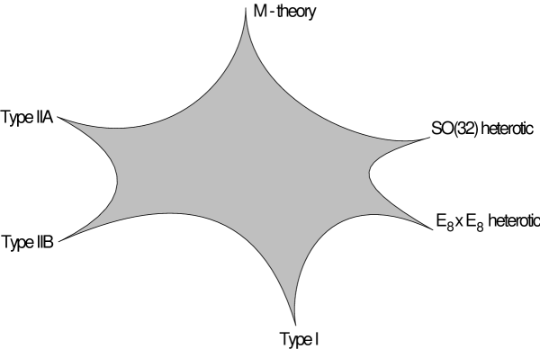
Figure 4.2: The moduli space of superstring theory.

There are two things to say about this picture. First of all the picture – as it comes from duality – is conjectural. There are no ”proofs” of these duality conjectures but only a number of consistency checks. However, so far there seems to be no inconsistencies. Secondly, it is only certain regions of the moduli space which is covered by known theories – so there is no fundamental definition of the theory behind all this (if it is unique).

M as in Matrix?

One attempt in the direction of giving a non-perturbative definition of $M$-theory is the Matrix Theory conjecture by Banks, Fischler, Shenker and Susskind [8] (and is reviewed in [128, 129]). It states that $M$-theory in the so-called infinite momentum frame (IMF) is described by a supersymmetric $U(N)$ Yang-Mills theory in $1+0$ dimensions. In a certain limit $N$ can be identified with the number of D0-branes and should be taken to infinity. The IMF is constructed as follows. Start with a state of energy $E$ in $M$-theory and consider a boost in the eleventh direction such that $p_{10}$ is large compared to any other scale in the theory. The energy is in this limit accordingly:

$$E=\sqrt{p_{10}^{2}+p_{\perp}^{2}+m^{2}}=p_{10}+\frac{p_{\perp}^{2}+m^{2}}{2p_{10}}\ .$$ (4.52)

Compactifying the theory – in the $x_{10}$-direction – on a circle of radius $R$ relates it to the Type IIA theory with

$$E=\frac{N}{R}+\frac{R(p_{\perp}^{2}+m^{2})}{2N}\ ,$$ (4.53)

and the first term on the right hand side is identified with the mass of $N$ D0-brane, as discussed earlier. The action describing the interaction of such $N$ D0-branes is a $U(N)$ supersymmetric Yang-Mills theory (4.10) reduced to the worldvolume of the D0-brane which is one-dimensional. In this way one gets a $U(N)$ quantum mechanics with an action like

$$S=\frac{1}{4g_{YM}^{2}}\int dt\ [2(D_{0}X^{i})^{2}+([X^{i},X^{j}])^{2}+{\rm fermions}]\ .$$ (4.54)

By dimensional reduction $F_{ij}=[X^{i},X^{j}]$ and $F_{0j}=D_{0}X^{j}=\partial_{0}X^{j}+[A_{0},X^{j}]$ with $X^{i}$ nine $N\times N$ matrices in the adjoint of $U(N)$. When the commutator-term in (4.54) vanish, these matrices can be simultaneously diagonalized and the diagonal elements are then identified with the positions of the $N$ D0-branes.

To obtain eleven-dimensional $M$-theory, we must take the limit $R\rightarrow\infty$ and therefore also $N\rightarrow\infty$.

This basically constitutes the definition of Matrix Theory. Subsequently, Matrix Theory has been compared with ”experiment”. As an example, the scattering of two gravitons has been computed to two-loop order (in the gauge coupling) in [130] and is found to agree with calculations from supergravity. The same conclusion have recently been shown to hold also in the case of three-graviton scattering [131].

It would of course be nice if this approach to $M$-theory could elucidate anything interesting about four-dimensional theories. Compactification of Matrix Theory gives gauge theories in higher dimensions (compactifying $d$ dimensions results in a $(d+1)$-dimensional gauge theory), but for $d>3$ they turn out not to be renormalizable. So the connection to four-dimensional field theories seems problematic. As another related problem we could mention that the large $N$ limit of Matrix Theory is not very well understood.

Such problems make the Matrix Theory approach to $M$-theory less appealing. It might, however, be possible that further study of the relation between this approach and the Maldacena approach – to be described below – can lead to a better understanding of certain aspects of Matrix Theory, e.g. of the large $N$ limit.

M as in Maldacena?

An – a priori – very different approach to $M$-theory is the recent Maldacena conjecture [1] (see [132] for an extensive review and references). By studying D-brane scattering Maldacena formulated a series of conjectures that relates Type IIB theory on Anti-de Sitter spaces to conformal field theories. As an example, with the geometry of $N$ D3-branes in Type IIB string theory, it is conjectured that Type IIB string theory on $AdS_{5}\times{\bf S}^{5}$ is equivalent to ${\cal N}=4$ supersymmetric $SU(N)$ Yang-Mills theory in $3+1$ dimensions! It is not obvious how a string theory in ten dimensions can be dual to a field theory in four dimensions. But at least it is easy to see that the bosonic symmetries match: the conformal group in four dimensions is $SO(2,4)$ and this is the same as the symmetry group of $AdS_{5}$ (the global bosonic symmetry groups are $SO(2,4)\times SO(6)$).

Subsequently, this conjecture has been made more precise [133] and in general terms it states that $M$-theory compactified on $AdS_{d+1}$ is dual to a conformal field theory on the boundary $S^{d}$ of this space.

If, for example, $\phi$ is a massless scalar field in $AdS_{d+1}$ with boundary value $\phi_{0}$, then it couples to an operator ${\cal O}$ (of conformal dimension $d$) in the conformal field theory such that,

$$Z_{SUGRA}(\phi|_{\partial AdS}=\phi_{0})=\langle e^{\int d^{d}x\phi_{0}{\cal O}}\rangle_{CFT}\ .$$ (4.55)

On the left hand side the partition function is computed in $AdS$-space and is identified on the right hand side with a correlator in the boundary conformal field theory.

As mentioned in the introduction, it has also been shown that this correspondence satisfies an interesting holographic bound [9]: the bulk spacetime theory is described by a boundary field theory which has at the most one degree of freedom per Planck area.

The $AdS$-space appears because in the so-called near-horizon limit the geometry of for example $N$ D3-branes is [1]:

$$ds^{2}=\alpha^{\prime}\left[\frac{U^{2}}{g_{YM}N^{1/2}}dx_{\parallel}^{2}+\frac{g_{YM}N^{1/2}}{U^{2}}(dU^{2}+U^{2}d\Omega_{5}^{2})\right]\ ,$$ (4.56)

in which the first two terms can be seen as a standard metric on $AdS_{5}$ ($x_{\parallel}$ are coordinates on the worldvolume of the D3-brane, $U=r/\alpha^{\prime}$ a radial coordinate, and $d\Omega_{5}^{2}$ is a metric on the unit five-sphere). Here the Yang-Mills coupling is related to the string coupling through

$$g=g_{YM}^{2}\ ,$$ (4.57)

and is related to the radius of the ${\bf S}^{5}$ according to

$$\frac{R}{\sqrt{\alpha^{\prime}}}=(4\pi g_{YM}^{2}N)^{1/4}\ .$$ (4.58)

For supergravity to be valid the radius $R$ should be large (so that curvatures are small) compared to the string scale; that is, one must have $gN\gg 1$. (In this sense the conjectured correspondence is a form of strong-weak coupling duality). For fixed $g$ one should therefore consider a limit $N\rightarrow\infty$, much as in Matrix Theory. But the interpretation of these limits is of course very different in the two theories.

It should be noted that the Maldacena conjecture not only gives an interesting approach to studying $M$-theory, but also to quantum field theory. For example in certain limits on one side of the correspondence one has supergravity compactified on $AdS$-space and on the other side a quantum field theory. In this manner one can learn about strongly coupled quantum field theory in e.g. four dimensions by studying supergravity. But also theories with even less supersymmetry can be studied. For example, it has been shown [134] that four-dimensional ${\cal N}=0$ $SU(N)$ gauge theory has a dual formulation in terms of $M$-theory on $M_{7}\times{\bf S}^{4}$, where $M_{7}$ is a certain seven-dimensional manifold.

This would mean that the distinction between quantum field theories and string/$M$-theory might not be so fundamental after all.

4.4 Some Consequences of String Duality in $D=4$

We will end this chapter by mentioning two examples where the conjectured duality relations between ten-dimensional string theories, and recent understanding of D-brane physics, have been connected to four-dimensional physics. The main idea here being that if we believe that the dualities relating the different string theories and $M$-theory in ten dimensions are correct, their implications in lower dimensions can be inferred by compactification.

First we look at the field theory Montonen-Olive duality (which was mentioned in the introduction) in four dimensions.

Montonen-Olive Duality in $D=4$

Starting with the conjectured $SL(2,{\bf Z})$ duality of Type IIB theory, one can study its consequences in lower dimensions. The Montonen-Olive duality of $D=4$ ${\cal N}=4$ $U(n)$ gauge theory can for example be derived from the duality in ten dimensions [122, 135].

The basic idea is as follows. The Type IIB theory has D3-branes. The world volume theory of $n$ D3-branes in Type IIB theory is a $D=4$ ${\cal N}=4$ $U(n)$ gauge theory, since reducing the ${\cal N}=1$ super Yang-Mills theory in ten dimensions to four dimensions gives ${\cal N}=4$ supersymmetry [36]. The gauge coupling is related to the string coupling through (4.11), or

$$g_{YM}^{2}=2\pi g\ ,$$ (4.59)

where $g$ is the string coupling and $g_{YM}$ the Yang-Mills gauge coupling. Now, the $SL(2,{\bf Z})$ symmetry of the Type IIB theory keeps the D3-brane invariant but changes the string coupling as $g\rightarrow 1/g$, the last because of $S$-duality corresponding to the transformation $\tau\rightarrow-1/\tau$. Then

$$g_{YM}^{2}\rightarrow 4\pi^{2}/g_{YM}^{2}\ ,$$ (4.60)

which is the transformation of the Yang-Mills coupling under Montonen-Olive duality. Similarly, one can derive the shift of the vacuum angle $\theta\rightarrow\theta+2\pi$ as coming from the shift of the axion (that is the R-R field $C_{0}$) in the Type IIB theory.

Thus, if $SL(2,{\bf Z})$-duality of the IIB string is correct it follows that the ${\cal N}=4$ supersymmetric Yang-Mills theory in four dimensions has a Montonen-Olive duality. Turning the argument around, if we think that Montonen-Olive duality is correct something must be right about the conjectured self-duality of the Type IIB theory.

This argument, however, is not very strong since there could be many different ways to “derive” Montonen-Olive duality in four dimensions from string theory (see e.g. [136] for another realization of Montonen-Olive duality).

Seiberg-Witten Duality in $D=4$

Seiberg-Witten duality has been identified as a consequence of duality of Type II theories in [137]. Introductions to the string theory construction of the ${\cal N}=2$ gauge theories can be found in [138, 139].

In turning to the string theory realization of Seiberg-Witten theory, the first question that comes to mind is the following. In the Seiberg-Witten solution, the prepotential ${\cal F}$ (in Eq. (2.63)) is determined by the period integrals of a certain meromorphic one-form $\lambda$ (2.65) on the basic cycles of the torus, or Seiberg-Witten curve, $\Sigma$ (2.64). Is there a concrete physical meaning of this curve?

In one construction [111] of the ${\cal N}=2$ theory the answer is simply that in Type IIA theory the worldvolume of a certain five-brane is $\Sigma\times{\bf R}^{4}$ and that the ${\cal N}=2$ effective field theory comes from the low energy Lagrangian of this five-brane theory.

In order to construct a four-dimensional theory one can compactify Type IIA theory on a six-dimensional Calabi-Yau manifold $X_{3}$, which should be such that we get a theory with ${\cal N}=2$ supersymmetry in four dimensions. For example, compactifying Type IIA on ${\bf T}^{6}$ would give a theory of ${\cal N}=8$ supersymmetry.

More concretely, $X_{3}$ is taken to be locally of the form ${\bf P}^{1}\times K3$. Here ${\bf P}^{1}$ is complex one-dimensional projective space (topologically ${\bf S}^{2}$) and $K3$ is a compact complex Kähler manifold of real dimension four with vanishing first Chern class and $h^{1,0}=0$ [141]. However, to preserve the Calabi-Yau condition, $X_{3}$ cannot be globally a product manifold. One says that $K3$ is fibered over ${\bf P}^{1}$, where ${\bf P}^{1}$ is the base geometry.

In order to identify the four-dimensional ${\cal N}=2$ theory, one can start with the compactification of Type IIA on a $K3$ manifold $X_{2}$. The R-R three-form $C_{3}$ in the Type IIA theory gives rise to the vector multiplet $A^{a}$ as $C_{3}\rightarrow A^{a}\wedge\omega^{a}$, where $\omega^{a}$ is a basis of $H^{2}(X_{2})$ [136]. Charged fields are obtained by wrapping $D2$-branes on two-cycles $S_{2}^{a}$ dual to the two-forms $\omega_{a}$. These become identified with the $W^{\pm}$ massive gauge multiplets that have masses proportional to the volume of the two-cycles $S_{2}$ (wrapping four-branes on four-cycles gives the corresponding magnetic duals).

To decouple gravity, that is to obtain a quantum field theory, these cycles must be vanishing. This is because in the decoupling limit one should take $\alpha^{\prime}\rightarrow 0$, while keeping the $W^{\pm}$ boson masses $\sim\alpha^{\prime-1/2}$ finite – it therefore turns out [136] that the local geometry becomes singular. Generally (that is for general gauge groups) the local geometry is that of an ALE (Asymptotically Locally Euclidean) space with so-called ADE Type singularities (see e.g. [141] for further discussion).

So the classical $SU(2)$ Yang-Mills theory is constructed by compactifying Type IIA string theory on ${\bf P}^{1}\times K3$ with local singular geometry.

However, in the Seiberg-Witten solution, the prepotential ${\cal F}$ has also an infinite series of instanton corrections [138]. How does one determine these in the string theory construction? One possibility is to use mirror symmetry [140] which will relate Type IIA on $X_{3}$ to Type IIB theory compactified on its mirror $\tilde{X_{3}}$ and with Kähler structure and complex structure interchanged.

The Calabi-Yau three-manifold can be characterized by Kähler structure and complex structure moduli. If $S_{2}^{a}$ is a basis of $H_{2}(X_{3})$ and $J$ is the Kähler form , then $t_{a}=\int_{S_{2}^{a}}J$ parametrizes the Kähler moduli space. The complex structure moduli space is parametrized by complex numbers $z_{i}$; here, if $S_{3}^{i}$ is a basis of $H_{3}(X_{3})$ and $\Omega$ is the unique three-form on $X_{3}$, then $z_{i}=\int_{S_{3}^{i}}\Omega$.

In the Type IIA theory the scalars of the vector multiplets (containing gauge fields and gauginos) are determined by the Kähler structure and those of the hyper multiplets (containing matter fields) by the complex structure. In the Type IIB theory the situation is reversed: the vector multiplet scalars are determined by the complex structure and the hyper multiplets by the Kähler structure.

The instanton corrections are so-called worldsheet instanton corrections – in the IIA theory they can be understood as coming from the wrapping of the string worldsheet on the base manifold ${\bf P}^{1}$. Since there is no neutral coupling between hypermultiplets and vector multiplets in the ${\cal N}=2$ theory only vector multiplets are important for determining these corrections.

So, in the Type IIB theory – where things are reversed – there are no worldsheet instanton corrections to the vector multiplet. This implies [136] that the classical period integrals $\int\Omega$ in $\tilde{X}_{3}$ describe the exact vector multiplet moduli space in the ${\cal N}=2$ theory. The general solution to the ${\cal N}=2$ theory is, therefore, given in terms of period integrals $\int_{S_{3}^{i}}\Omega$ on a local Calabi-Yau geometry in $\tilde{X}_{3}$.

The period integrals of the meromorphic one-form $\lambda$ on the Seiberg-Witten curve $\Sigma$ can then be obtained by ’integrating out’ the two extra dimensions on a certain two-cycle $S_{2}$. In this way, one can get an explicit representation of the Seiberg-Witten curve (2.64) as determined by the local geometry of the Calabi-Yau manifold $\tilde{X}_{3}$ [137].

In this representation, one can also compute the stable BPS spectrum in a rather simple way – something which usually is quite hard from the quantum field theory point of view.

Finally, let us mention, that there is a third representation of the ${\cal N}=2$ theory. This is obtained by using a $T$-duality, which maps Type IIB in the neighbourhood of an $A_{1}$ singularity of ALE space to Type IIA on a symmetric five-brane [139]. The worldvolume of this five-brane is $\Sigma\times{\bf R}^{4}$. Compactifying the resulting theory on $\Sigma$ gives a four-dimensional ${\cal N}=2$ theory which is identified with the low energy effective theory of the Seiberg-Witten solution [111].

Having sketched how the Seiberg-Witten duality (which played an important role in the topological field theories studied in our first chapter) in four dimensions follows naturally from string duality in ten dimensions, we believe this is a natural place to end.

Chapter 5 Discussion

We have studied aspects of duality in various situations: in topological field theory (as the Seiberg-Witten duality), in field theory (as the $T$-duality of sigma models) and in string theory (where duality seems to connect all five known theories in ten dimensions).

In testing dualities the topological field theory approach seems to be an important one. Not only because topological field theories are very simple but also because one might hope that the results that follow from using the Seiberg-Witten invariants can be proven in an exact way.

In this thesis we have shown that by dimensionally reducing the topological field theories corresponding to the two (dual) approaches to Donaldson theory, one obtains theories which by construction are topological, and we have derived the corresponding ”monopole” equations in three and two dimensions [19]. While the three-dimensional versions have been studied quite extensively in the literature, there is still a gap to be filled in the two-dimensional case. Here one studies what are called the Hitchin equations on a Riemann surface. The connection from duality in moduli space could in principle be used to carry out an analysis from the point of view of the Seiberg-Witten theory. To this end, the vanishing theorems we derived in two dimensions should be important.

Even in the original four-dimensional effective ${\cal N}=2$ theory do such two-dimensional topological field theories appear to play a role. In two-dimensional Landau-Ginzburg models, the three-point correlators can be shown to obey the so-called WDVV (Witten-Dijkgraaf-Verlinde-Verlinde) equations. As discussed in [142], the same equations have been shown to hold for certain derivatives of the prepotential, which seem to indicate that the low-energy effective theory contains a certain two-dimensional topological structure.

It is important to establish whether the two-dimensional topological field theory obtained by dimensionally reducing the monopole action is in any way connected to the WDVV equations.

Also, since everything is rather simple in two dimensions, one might speculate that duality can be derived more directly. Here the connection to string theory is also important; it is quite likely that string theory will provide a new understanding of the relations between invariants of various moduli spaces. Hence, it would be interesting to study the moduli problems from the point of view of non-perturbative string theory. This does not seem an impossible task. It is well known that topological quantum field theories (at least those associated with ${\cal N}=4$ supersymmetry) can be obtained from D-branes in string theory [143].

One might also speculate about getting interesting topological field theory dualities from the Maldacena conjecture [1]. According to this conjecture, a conformal field theory in $d$ dimensions is described by Type IIB string theory compactified on ($d+1$)-dimensional Anti-de Sitter space (on the boundary of which the field theory resides). Twisting the conformal field theory, one should obtain a $d$-dimensional topological field theory which is dual to a certain string theory in $d+1$ dimensions! Could this be important for studying the topology of four-manifolds?

We then studied some restrictions imposed by $T$-duality in two-dimensional sigma models. The key result here is the relation, put forward by the author and P. Haagensen, that at any order in sigma model perturbation theory the RG flow (as denoted by the operator $R$) commute with $T$-duality: $[T,R]=0$ [72]. This has been verified to leading order in $\alpha^{\prime}$ – for bosonic, supersymmetric and heterotic sigma models [72, 73, 74]. The validity has also been demonstrated to second order in $\alpha^{\prime}$ for bosonic models with a purely metric background [72]. It seems natural to generalize this latter result to the case of torsionful backgrounds even though there here is the further complication of scheme dependence.

Also, starting with $[T,R]=0$, we have been able to essentially compute the one-loop beta functions in these models, and the two-loop functions in the case of bosonic and supersymmetric models with purely metric backgrounds [74].

Recently Balog et al. [80] have presented a derivation of $[T,R]=0$ at one-loop order, which explains (at least to one-loop order) why we have found the consistency conditions studied in Chapter 3 being exactly satisfied for the Weyl anomaly coefficients. This work naturally calls for a generalization to higher-loop orders. In this way one should be able to address the question of corrections to duality at two-loop order including the antisymmetric tensor background [83].

It has also turned out that a requirement such as $[T,R]=0$, with $T$ some duality symmetry, not only provides constraints on RG flow in sigma models but also in models with $S$-duality and statistical systems [76, 78]. But in these cases it needs to be identified what principles are needed to ask for commutativity between RG flow and dualities in the first place. In this context, we also propose to study further such relations between duality and RG flow for the open string sigma models, here with the ingredient of D-branes added.

Finally, we have tried to give an outline of the present status of string theory duality in ten dimensions. Here it has turned out that all ten-dimensional theories are connected in a manner such that the strong coupling limit of any of these five theories has a corresponding naturally weakly coupled theory (many similar results have been obtained in lower dimensions as is apparent from [7] and its citations). Most surprising is the Type IIA theory where one gets an eleven-dimensional theory, called $M$-theory (note that all other theories can be obtained as certain limits of $M$-theory). While we do not know the correct way to formulate $M$-theory or what the relevant degrees of freedom are, we do know that in superstring theory D-branes play a central role in describing the dynamics at strong coupling. Hence, they seem to be important in finding the right way to formulate string/$M$-theory. As such they have played an important role both in the formulation of the Matrix Theory conjecture and in the more recent Maldacena conjecture. And in the latter case there is even the added bonus that one can make certain predictions about quantum field theories at strong coupling.

Let us conclude by saying that duality still has not fully answered the more fundamental questions such as: ”what is field theory?”, ”what is string theory?” or ”what is $M$-theory?”. But at least we seem to be on the way.

Appendix A Kaluza-Klein Reduction

We write a generic background metric $g_{\mu\nu}$ as in (3.84) , and the components of the antisymmetric background tensor $b_{\mu\nu}$ as $b_{0i}\equiv w_{i}$ and $b_{ij}$. In this notation, barred quantities refer to the metric $\bar{g}_{ij}$.

• Inverse metric: $g^{00}\!=\!1/a+v_{i}v^{i},\ g^{0i}\!=\!-v^{i},\ g^{ij}\!=\!\bar{g}^{ij}$. On decomposed tensors, indices $i,j,\ldots$ are raised and lowered with the metric $\bar{g}_{ij}$ and its inverse. With the metric decomposition (3.84) we also have $\det g=a\det\bar{g}$.

• Connection coefficients:

  $$\Gamma^{0}_{00} = {a\over 2}v^{i}a_{i}\ ,\ \Gamma^{0}_{i0}={a\over 2}\left[{a_{i}\over a}+v^{j}a_{j}v_{i}+v^{j}F_{ji}\right]\ ,$$

  $$\Gamma^{i}_{00} = -{a\over 2}a^{i}\ ,\ \Gamma^{i}_{0j}=-{a\over 2}\left[F^{i}_{\ j}+a^{i}v_{j}\right]\ ,$$

  $$\Gamma^{0}_{ij} = -\bar{\Gamma}^{k}_{ij}v_{k}+{1\over 2}(\partial_{i}v_{j}+\partial_{j}v_{i}+a_{i}v_{j}+a_{j}v_{i})-{a\over 2}v^{k}\left[v_{j}F_{ik}+v_{i}F_{jk}-a_{k}v_{i}v_{j}\right]\ ,$$

  $$\Gamma^{i}_{jk} = \bar{\Gamma}^{i}_{jk}+{a\over 2}\left[v_{j}F_{k}^{\ i}+v_{k}F_{j}^{\ i}-a^{i}v_{j}v_{k}\right]\ ,$$ (A.1)

  where $a_{i}\!=\!\partial_{i}\ln a\ ,\ F_{ij}\!=\!\partial_{i}v_{j}-\partial_{j}v_{i}$.

• Ricci tensor:

  $$R_{00} = -{a\over 2}\left[\bar{\nabla}_{i}a^{i}+{1\over 2}a_{i}a^{i}-{a\over 2}F_{ij}F^{ij}\right]\ ,$$

  $$R_{0i} = v_{i}R_{00}+{3a\over 4}a^{j}F_{ij}+{a\over 2}\bar{\nabla}^{j}F_{ij}\ ,$$

  $$R_{ij} = \bar{R}_{ij}+v_{i}R_{0j}+v_{j}R_{0i}-v_{i}v_{j}R_{00}-{1\over 2}\bar{\nabla}_{i}a_{j}-{1\over 4}a_{i}a_{j}-{a\over 2}F_{ik}F_{j}^{\ k}\ .$$ (A.2)

• Riemann tensor:

  $$R_{i0k0} = -{a\over 2}\left({1\over 2}a_{i}a_{k}+\bar{\nabla}_{i}a_{k}+{a\over 2}F_{i}^{\ l}F_{lk}\right)\ ,$$

  $$R_{ijk0} = v_{j}R_{i0k0}-v_{i}R_{j0k0}-{a\over 2}\bar{\nabla}_{k}F_{ij}-{a\over 2}\left(a_{k}F_{ij}+{1\over 2}a_{j}F_{ik}-{1\over 2}a_{i}F_{jk}\right)\ ,$$

  $$R_{ijkm} = \bar{R}_{ijkm}+R_{ijk0}v_{m}+R_{jim0}v_{k}+R_{mkj0}v_{i}+R_{kmi0}v_{j}\ ,$$ (A.3)

  $$\ -R_{m0j0}v_{i}v_{k}+R_{k0j0}v_{i}v_{m}-R_{k0i0}v_{j}v_{m}+R_{m0i0}v_{j}v_{k}\ ,$$

  $$\ -{a\over 4}\left(F_{im}F_{kj}+F_{ki}F_{mj}+2F_{ji}F_{mk}\right).$$

• Torsion:

  $$H_{0ij} = -\partial_{i}w_{j}+\partial_{j}w_{i}\equiv-G_{ij}\ ,$$

  $$H_{ijk} = \partial_{i}b_{jk}+\partial_{j}b_{ki}+\partial_{k}b_{ij}\ ,$$ (A.4)

  and all other components vanish. For the one-loop beta function the following quantities are needed:

  $$H_{0\mu\nu}H_{0}^{\ \mu\nu} = G_{ij}G^{ij}\ ,$$

  $$H_{0\mu\nu}H_{i}^{\ \mu\nu} = -2G_{ij}G^{jk}v_{k}-H_{ijk}G^{jk}\ ,$$

  $$H_{i\mu\nu}H_{j}^{\ \mu\nu} = 2\left({1\over a}+v_{m}v^{m}\right)G_{i}^{\ k}G_{jk}-2v^{k}v^{m}G_{ik}G_{jm}+2H_{km(i}G_{j)}^{\ k}v^{m}$$ (A.5)

  $$+H_{ikm}H_{j}^{\ km}\ ,$$

  and

  $$\nabla_{\mu}H^{\mu}_{\ 0i} = \bar{\nabla}^{j}G_{ji}-aG_{ij}F^{jk}v_{k}+{1\over 2}G_{ij}a^{j}-{a\over 2}F^{jk}\left(H_{ijk}+v_{i}G_{jk}\right)\ ,$$

  $$\nabla_{\mu}H^{\mu}_{\ ij} = \bar{\nabla}^{k}\left(H_{kij}+v_{k}G_{ij}\right)-{1\over 2}\left[G_{i}^{\ k}\bar{\nabla}_{(k}\ v_{j)}-G_{j}^{\ k}\bar{\nabla}_{(k}\ v_{i)}\right]-{a\over 2}v_{[i}H_{j]km}F^{km}$$ (A.6)

  $$+v_{[i}G_{j]k}\left(a^{k}-aF^{km}v_{m}\right)+{1\over 2}a^{k}H_{kij}+{1\over 2}v_{m}a^{m}G_{ij}-{1\over 2}F_{[i}^{\ k}G_{j]k}\ ,$$

  where $[ij]=ij-ji$ and $(ij)=ij+ji$.

• Dilaton terms:

  $$\nabla_{0}\partial_{0}\phi = {a\over 2}a^{i}\partial_{i}\phi\ ,$$

  $$\nabla_{0}\partial_{i}\phi = {a\over 2}\left(F^{j}_{\ i}+a^{j}v_{i}\right)\partial_{j}\phi\ ,$$

  $$\nabla_{i}\partial_{j}\phi = \bar{\nabla}_{i}\partial_{j}\phi-{a\over 2}\left(v_{i}F_{j}^{\ k}+v_{j}F_{i}^{\ k}-a^{k}v_{i}v_{j}\right)\partial_{k}\phi\ .$$ (A.7)

• Tangent space geometrical tensors:

  When referred to the tangent space, the Ricci tensor becomes

  $$R_{\hat{0}\hat{0}} = -{1\over 2}\left[\bar{\nabla}_{i}a^{i}+{1\over 2}a_{i}a^{i}-{a\over 2}F_{ij}F^{ij}\right]\ ,$$

  $$R_{\hat{0}\alpha} = \bar{e}^{\ i}_{\alpha}\left[{3\sqrt{a}\over 4}a^{j}F_{ij}+{\sqrt{a}\over 2}\bar{\nabla}^{j}F_{ij}\right]\ ,$$

  $$R_{\alpha\beta} = \bar{e}^{\ i}_{\alpha}\bar{e}^{\ j}_{\beta}\left[\bar{R}_{ij}-{1\over 2}\bar{\nabla}_{i}a_{j}-{1\over 4}a_{i}a_{j}-{a\over 2}F_{ik}F_{j}^{\ k}\right]\ ,$$ (A.8)

  where $\bar{e}^{\ i}_{\alpha}$ is the inverse vielbein for the metric $\bar{g}_{ij}$. Likewise, the Riemann tensor is

  $$R_{\alpha\hat{0}\beta\hat{0}} = -{1\over 2}\bar{e}^{\ i}_{\alpha}\bar{e}^{\ j}_{\beta}\left({1\over 2}a_{i}a_{j}+\bar{\nabla}_{i}a_{j}+{a\over 2}F_{i}^{\ s}F_{sj}\right)\ ,$$

  $$R_{\alpha\beta\gamma\hat{0}} = -{\sqrt{a}\over 2}\bar{e}^{\ i}_{\alpha}\bar{e}^{\ j}_{\beta}\bar{e}^{\ k}_{\gamma}\left(a_{k}F_{ij}+{1\over 2}a_{j}F_{ik}-{1\over 2}a_{i}F_{jk}+\bar{\nabla}_{k}F_{ij}\right)\ ,$$

  $$R_{\alpha\beta\gamma\delta} = \bar{e}^{\ i}_{\alpha}\bar{e}^{\ j}_{\beta}\bar{e}^{\ k}_{\gamma}\bar{e}^{\ m}_{\delta}\left(\bar{R}_{ijkm}-{a\over 4}(F_{im}F_{kj}+F_{ki}F_{mj}+2F_{ji}F_{mk})\right).$$ (A.9)

Appendix B Two-Loop Tensor Structures

The possible tensor structures which can appear at two-loop are symmetric tensors and must scale as $\Omega^{-1}$ under global scalings of the background metric. A moment of thought reveals that the structure of the terms can be only of the three following kinds: $\nabla_{\cdot}\nabla_{\cdot}R_{\cdot\cdot\cdot\cdot}$, $R_{\cdot\cdot\cdot\cdot}R_{\cdot\cdot\cdot\cdot}$ or $g_{\mu\nu}\times$(traces of the previous tensors). Here the $\cdot$ indicates a $\mu$, $\nu$ index or a contracted index; $R_{\cdot\cdot\cdot\cdot}$ is the Riemann tensor. The resulting tensors are:

• Tensors of the form $\nabla_{\cdot}\nabla_{\cdot}R_{\cdot\cdot\cdot\cdot}$:

  $$\nabla_{\mu}\nabla_{\mu}R,\nabla^{2}R_{\mu\nu},\ \nabla_{(\mu}\nabla_{\alpha}R^{\alpha\ \ \ \beta}_{\ \beta\nu)},\ \nabla_{\alpha}\nabla_{(\mu}R^{\alpha\ \ \ \beta}_{\ \beta\nu)},\ \nabla_{\alpha}\nabla_{\beta}R^{\alpha\ \ \beta}_{\ (\mu\ \nu)}$$ (B.1)

• Tensors of the form $R_{\cdot\cdot\cdot\cdot}R_{\cdot\cdot\cdot\cdot}$:

  $$R_{\mu\alpha\nu\beta}R^{\alpha\beta},\ R_{\mu\alpha\beta\gamma}R_{\nu}^{\ \alpha\beta\gamma},\ R_{\mu\gamma\alpha\beta}R_{\nu}^{\ \alpha\beta\gamma},\ R_{\mu\alpha\beta\gamma}R_{\nu}^{\ \gamma\alpha\beta},$$

  $$R_{\mu\gamma\alpha\beta}R_{\nu}^{\ \gamma\alpha\beta},\ R_{\mu\alpha}R_{\nu}^{\ \alpha},\ R_{\mu\nu}R$$ (B.2)

• Tensors of the form $g_{\mu\nu}\times$(traces):

  $$g_{\mu\nu}\nabla^{2}R,\ g_{\mu\nu}\nabla_{\alpha}\nabla_{\beta}R^{\alpha\beta},\ g_{\mu\nu}R^{2},\ g_{\mu\nu}R_{\alpha\beta}R^{\alpha\beta},\ g_{\mu\nu}R_{\alpha\beta\gamma\delta}R^{\alpha\beta\gamma\delta}$$

  $$g_{\mu\nu}R_{\alpha\beta\gamma\delta}R^{\alpha\gamma\delta\beta}$$ (B.3)

Here we have reduced from a larger set by using the known symmetries of the Riemann tensor. As described in the main text only 10 of these 18 tensors are linearly independent. To show linear dependence between different tensors one uses the first and second Bianchi identities and the expression for $[\nabla,\nabla]$ acting on tensors. The first Bianchi identity determines for example that

$$R_{\mu\alpha\beta\gamma}R_{\nu}^{\ \alpha\beta\gamma}=-R_{\mu\alpha\beta\gamma}R_{\nu}^{\ \gamma\alpha\beta}-R_{\mu\gamma\alpha\beta}R_{\nu}^{\ \alpha\beta\gamma},$$ (B.4)

while the second Bianchi identity implies that

$$g_{\mu\nu}\nabla_{\alpha}\nabla_{\beta}R^{\alpha\beta}={1\over 2}g_{\mu\nu}\nabla^{2}R\ .$$ (B.5)

Bibliography

- [1] J.M. Maldacena, The Large Limit Of Superconformal Field Theories And Supergravity, Adv. Theor. Math. Phys. 2 (1998) 231, hep-th/9711200.
- [2] N. Seiberg and E. Witten, Electric-Magnetic Duality, Monopole Condensation, And Confinement In Supersymmetric Yang-Mills Theory, Nucl. Phys. B426 (1994) 19, hep-th/9407087.
- [3] N. Seiberg and E. Witten, Monopoles, Duality And Chiral Symmetry Breaking In Supersymmetric QCD, Nucl. Phys. B430 (1994) 485, hep-th/9408099.
- [4] N. Seiberg, Electric-Magnetic Duality In Supersymmetric Non-Abelian Gauge Theories, Nucl. Phys. B435 (1995) 129, hep-th/9411149.
- [5] E. Witten, Monopoles And Four-Manifolds, Math. Res. Lett. 1 (1994) 769, hep-th/9411102.
- [6] J. Polchinski, Dirichlet-Branes And Ramond-Ramond Charges, Phys. Rev. Lett. 75 (1995) 4724, hep-th/951017.
- [7] E. Witten, String Theory Dynamics In Various Dimensions, Nucl. Phys. B433 (1995) 85, hep-th/9503124.
- [8] T. Banks, W. Fischler, S. Schenker and L. Susskind, -Theory As A Matrix Model: A Conjecture, Phys. Rev. D55 (1997) 5112, hep-th/9610043.
- [9] L. Susskind and E. Witten, The Holographic Bound In Anti-de Sitter Space, hep-th/9805114.
- [10] P.A.M. Dirac, Quantized Singularities In The Electromagnetic Field , Proc. Roy. Soc. A33 (1931) 60.
- [11] S. Coleman, Quantum Sine-Gordon Equation As The Massive Thirring Model, Phys. Rev. D11 (1975) 2088.
- [12] S. Mandelstam, Soliton Operators For The Quantized Sine-Gordon Equation, Phys. Rev. D11 (1975) 3026.
- [13] H.A. Kramers and G.H. Wannier, Statistics Of The Two-Dimensional Ferromagnet, Phys. Rev. 60 (1941) 252.
- [14] C. Montonen and D. Olive, Magnetic Monopoles As Gauge Particles, Phys. Lett. 72B (1977) 117.
- [15] E. Witten, Topological Quantum Field Theory, Comm. Math. Phys. 117 (1988) 353.
-
[16]
S. K. Donaldson,
An Application Of Gauge Theory To Four-Dimensional Topology,
J. Diff. Geom. 18 (1983) 279.
S. K. Donaldson, Polynomial Invariants For Smooth Four Manifolds, Topology 29 (1990) 257. - [17] C. Vafa and E. Witten, A Strong Coupling Test Of -Duality, Nucl. Phys. B431 (1994) 3, hep-th/9408074.
- [18] D. Birmingham, M. Blau, M. Rakowski and G. Thompson, Topological Field Theory, Phys. Rep. 209 (1991) 129.
- [19] K. Olsen, Dimensional Reduction Of Dual Topological Field Theories, Mod. Phys. Lett. A11 (1996) 1777, hep-th/9603023.
- [20] N.J. Hitchin, The Self-Duality Equations On A Riemann Surface, Proc. London Math. Soc. 3 (1987) 59.
- [21] E. Witten, Topological Sigma Models, Comm. Math. Phys. 118 (1988) 411.
- [22] E. Witten, Quantum Field Theory And The Jones Polynomial, Comm. Math. Phys. 121 (1989) 351.
- [23] M. Green, J. Schwarz and E. Witten, Superstring Theory, two volumes, Cambridge University Press (1987).
- [24] E. Witten, Introduction To Cohomological Field Theories, Int. J. Mod. Phys. A6 (1991) 2775.
- [25] E. Witten, Mirror Manifolds And Topological Field Theory, hep-th/9112056.
- [26] R. Dijkgraaf, Lectures On Four-Manifolds And Topological Gauge Theories, Nucl. Phys. (Proc. Suppl.) 45B C (1996) 29.
- [27] M. Nakahara, Geometry, Topology and Physics, IOP, (1990).
- [28] M.H. Freedman, The Topology Of 4-Dimensional Manifolds, Jour. Diff. Geom. 17 (1982) 357.
- [29] L. Baulieu and I.M. Singer, Topological Yang-Mills Symmetry, Nucl. Phys. B (Proc. Suppl.) 5B (1988) 12.
- [30] E. Witten, Supersymmetric Yang-Mills Theory On A Four-Manifold, J. Math. Phys. 35 (1994) 5101, hep-th/9403195.
- [31] J. Wess and J. Bagger, Supersymmetry And Supergravity, Princeton University Press (1992).
- [32] S. K. Donaldson, The Seiberg-Witten Equations And 4-Manifold Topology, Bull. Amer. Math. Soc. 33 (1996) 45.
- [33] G. Moore and E. Witten, Integration Over The -Plane In Donaldson Theory, hep-th/9709193.
- [34] C. Nash, Differential Topology And Quantum Field Theory, Academic Press, (1991).
- [35] A. Bilal, Duality In Susy Yang-Mills Theory: A Pedagogical Introduction To The Work Of Seiberg And Witten, hep-th/9601007.
- [36] P. Di Vecchia, Duality In Supersymmetric Gauge Theories, hep-th/9803026.
- [37] J.M.F. Labastida and M. Mariño, A Topological Lagrangian For Monopoles On Four-Manifold, Phys. Lett. B351 (1995) 146.
- [38] M. Marcolli, Notes On Seiberg-Witten Gauge Theory, dg-ga/9509005.
- [39] A.L. Carey, J. McCarthy, B.L. Wang and R.B. Zhang, Topological Quantum Field Theory And Seiberg-Witten Monopoles, hep-th/9504005.
- [40] M. Mariño, The Geometry Of Supersymmetric Gauge Theories In Four Dimensions, Ph.D. Thesis, hep-th/9701128.
- [41] J.M.F. Labastida, Topological Quantum Field theory: A Progress Report, hep-th/9511037.
- [42] J.M.F. Labastida and C. Lozano, Lectures On Topological Quantum Field Theory, hep-th/9709192.
- [43] P.B. Kronheimer and T.S. Mrowka, Recurrence Relations And Asymptotics For Four-Manifold Invariants, Bull. Am. Math. Soc. 30 (1994) 215.
- [44] P.B. Kronheimer and T.S. Mrowka, The Genus Of Embedded Surfaces In The Projective Plane, Math. Res. Lett. 1 (1994) 797.
- [45] G. Thompson, New Results In Topological Field Theory And Abelian Gauge Theory, hep-th/9511038.
- [46] D. Birmingham, M. Rakowski and G. Thompson, BRST Quantization Of Topological Field Theory, Nucl. Phys. B315 (1989) 577.
- [47] G. Chapline and B. Grossman, Conformal Field Theory And A Topological Quantum Theory Of Vortices And Knots, Phys. Lett. B223 (1989) 336.
- [48] L. Rozansky and E. Witten, Hyperkähler Geometry And Invariants Of Three-Manifolds, hep-th/9612216.
- [49] M. Mariño and G. Moore, 3-Manifold Topology And The Donaldson-Witten Partition Function, hep-th/9811214.
- [50] Y. Ohta, Topological Field Theories Associated With Three-Dimensional Seiberg-Witten Monopoles, Int. J. Theor. Phys. 37 (1998) 925, hep-th/9611120.
- [51] S. Nergiz and C. Saçhog̃lu, Liouville Vortex And Kink Solutions Of The Seiberg-Witten Equations, Jour. Math. Phys. 37 (1996) 3753. hep-th/9602088.
- [52] P.G.O. Freund, Dirac Monopoles And Witten’s Monopole Equations, Jour. Math. Phys. 36 (1995) 2673, hep-th/9412208.
- [53] M. Mariño and G. Moore, Donaldson Invariants For Non-Simply Connected Manifolds, hep-th/9804104.
-
[54]
C. Okonek and A. Teleman, Recent Developments In Seiberg-Witten
Theory And Complex Geometry, alg-geom/9612015.
A. Teleman, Moduli Space Of -Monopoles, dg-ga/9702006. - [55] A. Giveon, M. Porrati and E. Rabinovici, Target Space Duality In String Theory, Phys. Rept. 244 (1994) 77, hep-th/9401139.
-
[56]
K. Kikkawa and M. Yamasaki, Casimir Effects In Superstring Theories,
Phys. Lett. B149 (1984) 357.
N. Sakai and I. Senda, Vacuum Energies Of String Compactified On Torus, Prog. Theor. Phys. 75 (1986) 692. -
[57]
T.H. Buscher, A Symmetry Of The String
Background Field Equations, Phys. Lett. B194 (1987) 59.
T.H. Buscher, Path-Integral Derivation Of Quantum Duality In Nonlinear Sigma-Models, Phys. Lett. B201 (1988) 466. - [58] M. Rocek and E. Verlinde, Duality, Quotients, And Currents, Nucl. Phys. B373 (1992) 630.
- [59] M. Dine, P. Huet and N. Seiberg, Large And Small Radius In String Theory, Nucl. Phys. B322 (1989) 301.
- [60] J. Dai, R.G. Leigh and J. Polchinski, New Connections Between String Theories, Mod. Phys. Lett. A4, No. 21 (1989) 2073.
- [61] L. Alvarez-Gaumé, D.Z. Freedman and S. Mukhi, The Background Field Method And The Ultraviolet Structure Of The Supersymmetric Nonlinear -Model, Ann. Phys. 134 (1981) 85.
- [62] D.H. Friedan, Nonlinear Models In Dimensions, Ann. Phys. 163 (1985) 318.
- [63] H. Ooguri and Z. Yin, Lectures On Perturbative String Theories, hep-th/9612254.
- [64] J. Polchinski, What Is String Theory?, hep-th/9411028.
- [65] C.G. Callan, D. Friedan, E.J. Martinec and M.J. Perry, Strings In Background Fields, Nucl. Phys. B262 (1985) 593.
- [66] A.A. Tseytlin, Conformal Anomaly In A Two-Dimensional Sigma Model On A Curved Background And Strings, Phys. Lett. B178 (1986) 34.
- [67] A.A. Tseytlin, Sigma Model Weyl Invariance Conditions And String Equations Of Motion, Nucl. Phys. B294 (1987) 383.
- [68] G. Curci and G. Paffuti, Consistency Between The String Background Field Equation Of Motion And The Vanishing Of The Conformal Anomaly, Nucl. Phys. B286 (1987) 399.
- [69] R.M. Wald, General Relativity, The University of Chicago Press (1984).
- [70] E. Alvarez, L. Alvarez-Gaume and Y. Lozano, An Introduction To -Duality In String Theory, Nucl. Phys. Proc. Suppl. 41 (1995) 1, hep-th/9410237.
- [71] C.A. Lütken, Geometry Of Renormalization Group Flows Constrained By Discrete Global Symmetries, Nucl. Phys. B396 (1993) 670.
- [72] P.E. Haagensen and K. Olsen, -Duality And Two-Loop Renormalization Flows, Nucl. Phys. B504 (1997) 326, hep-th/9704157.
- [73] P.E. Haagensen, Duality Transformations Away From Conformal Points, Phys. Lett. B382 (1996) 356, hep-th/9604136.
- [74] P.E. Haagensen, K. Olsen and R. Schiappa, Two-Loop Beta Functions Without Feynman Diagrams, Phys. Rev. Lett. 79 (1997) 3573, hep-th/9705105.
- [75] K. Olsen and R. Schiappa, Heterotic -Duality And The Renormalization Group, Int. Jour. Mod. Phys. A114 (1999) 2257, hep-th/9805074.
- [76] P.H. Damgaard and P.E. Haagensen, Constraints On Beta Functions From Duality, Jour. Phys. A30 (1997) 4681, cond-mat/9609242.
- [77] C.P. Burgess and C.A. Lütken, One-Dimensional Flows In The Quantum Hall System, Nucl. Phys. B500 (1997) 367, cond-mat/9611118.
- [78] A. Ritz, On The Beta-Function In =2 Supersymmetric Yang-Mills Theory, Phys. Lett. B434 (1998) 54, hep-th/9710112.
- [79] J.I. Latorre and C.A. Lütken, On RG Potentials In Yang-Mills Theories, Phys. Lett. B421 (1998) 217, hep-th/9711150.
- [80] J. Balog, P. Forgács, N. Mohammedi, L. Palla and J. Schnittger, On Quantum -Duality In Models, Nucl. Phys. B535 (1998) 461, hep-th/9806068.
- [81] K.S. Narain, New Heterotic String Theories In Uncompactified Dimensions , Phys. Lett. B169 (1986) 41.
- [82] J. Maharana and J.H. Schwarz, Noncompact Symmetries In String Theory, Nucl. Phys. 390B (1993) 3.
-
[83]
N. Kaloper and K. A. Meissner, Duality
Beyond The First Loop,
Phys. Rev. D56 (1997) 7940, hep-th/9705193.
N. Kaloper and K. A. Meissner, Tailoring -Duality Beyond The First Loop, hep-th/9708169. - [84] P.E. Haagensen, Duality And The Renormalization Group, in the Proceedings of the NATO Workshop New Trends in Quantum Field Theory, Zakopane, Poland, 14-21 June 1997, ed. P.H. Damgaard (Plenum Press, 1997), hep-th/9708110.
- [85] A.A. Tseytlin, Duality And Dilaton, Mod. Phys. Lett. A6 (1991) 1721.
-
[86]
J. Balog, P. Forgács, Z. Horváth and L. Palla, Perturbative
Quantum (In)equivalence Of Dual Models In 2 Dimensions, hep-th/9601091;
J. Balog, P. Forgács, Z. Horváth and L. Palla, Quantum Corrections Of Abelian Duality Transformations, Phys. Lett. B388 (1996) 121, hep-th/9606187. - [87] R.R. Metsaev, A.A. Tseytlin, Order Alpha-Prime (Two Loop) Equivalence Of The String Equations Of Motion And The Sigma Model Weyl Invariance Conditions: Dependence On The Dilaton And The Antisymmetric Tensor, Nucl. Phys. B293 (1987) 385.
- [88] S.J. Gates, C.M. Hull and M. Rocek, Twisted Multiplets And New Supersymmetric Non-Linear -Models, Nucl. Phys. B248 (1984) 157.
- [89] B. Zumino, Supersymmetry And Kähler Manifolds, Phys. Lett. B87 (1979) 203.
-
[90]
L. Alvarez-Gaumé and D.Z. Freedman, Kähler
Geometry And The Renormalization Of Supersymmetric Sigma Models,
Phys. Rev. D22 (1980) 846.
L. Alvarez-Gaumé and D.Z. Freedman, Geometrical Structure And Ultraviolet Finiteness In The Supersymmetric Sigma Model, Comm. Math. Phys. 80 (1981) 443. - [91] M.F. Sohnius and P.C. West, Conformal Invariance In Supersymmetric Yang-Mills, Phys. Lett. B100 (1981) 245.
- [92] C.M. Hull and E. Witten, Supersymmetric Sigma Models And The Heterotic String, Phys. Lett. B160 (1985) 398.
- [93] D.J. Gross, J.A. Harvey, E. Martinec, and R. Rohm, The Heterotic String, Phys. Rev. Lett. 54 (1985) 502.
- [94] E. Alvarez, L. Alvarez-Gaumé and I. Bakas, -Duality And Space-Time Supersymmetry, Nucl. Phys. B457 (1995) 3, hep-th/9507112.
- [95] C.M. Hull, Gauged Heterotic Sigma Models, Mod. Phys. Lett. A9 (1994) 161, hep-th/9310135.
- [96] E. Alvarez, L. Alvarez-Gaumé and I. Bakas, Supersymmetry And Dualities, Nucl. Phys. Proc. Suppl. 46 (1996) 16, hep-th/9510028.
- [97] S. Bellucci and R.N. Oerter, Weyl Invariance Of The Green-Schwarz Heterotic Sigma Model, Nucl. Phys. B363 (1991) 573.
- [98] A. Giveon, E. Rabinovici and A.A. Tseytlin, Heterotic String Solutions And Coset Conformal Field Theories, Nucl. Phys. B409 (1993) 339, hep-th/9304155.
- [99] G. Grignani and M. Mintchev, The Effect Of Gauge And Lorentz Anomalies On The Beta Functions Of The Heterotic Sigma Model, Nucl. Phys. B302 (1988) 330.
- [100] A. Sen, Equations Of Motion For The Heterotic String Theory From The Conformal Invariance Of The Sigma Model, Phys. Rev. Lett. 55 (1985) 1846.
-
[101]
H. Dorn and H.J. Otto, Remarks On -Duality For
Open Strings, Nucl. Phys. Proc. Suppl. 56B (1997) 30-35, hep-th/9702018.
H. Dorn, The Mass Term In Non-Abelian Gauge Field Dynamics On Matrix D-Branes And -Duality In The -Model Approach, J.High Energy Phys. 04 (1998) 013, hep-th/9804065. -
[102]
M.T. Grisaru, A.E.M. Van De Ven and D. Zanon, Four-Loop Divergences For The And
Supersymmetric Non-Linear Sigma-Model In Two Dimensions,
Phys. Lett. B173 (1986) 423.
M.T. Grisaru, A.E.M. Van De Ven and D. Zanon, Four-Loop Divergences For The Supersymmetric Non-Linear Sigma-Model, Nucl. Phys. B277 (1986) 409. - [103] S. A. Fulling, R.C. King, B.G. Wybourne and C. J. Cummins, Normal Forms For Tensor Polynomials: I. The Riemann Tensor, Class. Quantum Grav. 9 (1992) 1151.
- [104] E. Kiritsis, Introduction To Superstring Theory, hep-th/9709062.
- [105] J. Polchinski, TASI Lectures On D-Branes, hep-th/9611050.
- [106] M. Duff, R.R. Khuri and J.X. Lu, String Solitons, Phys. Rep. 259 (1995) 213, hep-th/9412184.
- [107] E. Witten, Bound States Of Strings And p-Branes, Nucl. Phys. B460 (1996) 335, hep-th/9510135.
- [108] R.G. Leigh, Dirac-Born-Infeld Action From Dirichlet -Model, Mod. Phys. Lett. A4 (1989) 2767.
- [109] A. Strominger and C. Vafa, Microscopic Origin Of The Bekenstein-Hawking Entropy, Phys. Lett. B379 (1996) 99, hep-th/9601029.
- [110] C.G. Callan and J.M. Maldacena, D-Brane Approach To Black Hole Quantum Mechanics, Nucl. Phys. 472 (1996) 591, hep-th/9602043.
- [111] E. Witten, Solutions Of Four-Dimensional Field Theories Via Theory, Nucl. Phys. B500 (1997) 3, hep-th/9703166.
- [112] P.K. Townsend, Four Lectures On -Theory, hep-th/9612121.
- [113] E. Kiritsis, Introduction To Non-Perturbative String Theory, hep-th/9708130.
- [114] A. Sen, An Introduction To Non-Perturbative String Theory, hep-th/9802051.
- [115] C.M. Hull and P.K. Townsend, Unity Of Superstring Dualities, Nucl. Phys. B438 (1995) 109, hep-th/9410167.
- [116] J.H. Schwarz, Covariant Field Equations Of Chiral Supergravity, Nucl. Phys. B226 (1983) 269.
- [117] P.S. Howe and P.C. West, The Complete , Supergravity, Nucl. Phys. B238 (1984) 181.
-
[118]
E. Cremmer, B. Julia and J. Scherk, Supergravity In 11 Dimensions,
Phys. Lett. B76 (1978) 409.
I.C.G. Campbell and P.C. West, , Non-Chiral Supergravity And Its Spontaneous Compactification, Nucl. Phys. B243 (1984) 112. - [119] P.K. Townsend, The Eleven-Dimensional Supermembrane Revisited, Phys. Lett. B350 (1995) 184, hep-th/9501068.
- [120] S. Sethi and M. Stern, D-Brane Bound States Redux, Comm. Math. Phys. 194 (1998) 675, hep-th/9705046.
- [121] M. Porrati and A. Rozenberg, Bound States At Threshold In Supersymmetric Quantum Mechanics, Nucl. Phys. B515 (1998) 184, hep-th/9708119.
- [122] P.K. Townsend, D-Branes From -Branes, Phys. Lett. B373 (1996) 68, hep-th/9512062.
- [123] P.S. Aspinwall, Some Relationships Between Dualities In String Theory, Nucl. Phys. Proc. Suppl. 46 (1996) 30, hep-th/9508154.
- [124] J.H. Schwarz, An Multiplet Of Type IIB Superstrings, hep-th/9508143.
- [125] J. Polchinski and E. Witten, Evidence For Heterotic-Type I String Duality, Nucl. Phys. B460 (1996) 525, hep-th/9510169.
- [126] E. Witten, Small Instantons In String Theory Nucl. Phys. B460 (1996) 541, hep-th/9511030.
- [127] P. Horava and E. Witten, Heterotic And Type I String Dynamics From Eleven Dimensions, Nucl. Phys. B460 (1996) 506, hep-th/9510209.
- [128] D. Bigatti and L. Susskind, Review Of Matrix Theory, hep-th/9712072.
- [129] W. Taylor, Lectures On D-Branes, Gauge Theory And M(atrices), hep-th/9801182.
- [130] K. Becker and M. Becker, A Two-Loop Test Of M(atrix) Theory, Nucl. Phys. B506 (1997) 48, hep-th9705091.
- [131] M. Fabbrichesi, G. Ferretti and R. Iengo, Supergravity And Matrix Theory Do Not Disagree On Multi-Graviton Scattering, J. High. Energy. Phys. 06 (1998) 02, hep-th/9806018
- [132] O. Aharony, S.S. Gubser, J. Maldacena, H. Ooguri and Y. Oz, Large Field Theories, String Theory And Gravity, hep-th/9905111.
-
[133]
S.S. Gubser, I.R. Klebanov and A. M. Polyakov,
Gauge Theory Correlators From Non-Critical String Theory,
Phys. Lett. B428 (1998) 105,
hep-th/9802109
E. Witten, Anti-de Sitter Space And Holography, Adv. Theor. Math. Phys. 2 (1998) 253, hep-th/9802150. - [134] E. Witten, Anti-de Sitter Space, Thermal Phase Transition, And Confinement In Gauge Theories, Adv. Theor. Math. Phys. 2 (1998) 505, hep-th/9803131.
- [135] A. Tseytlin, Self-Duality Of Born-Infeld Action And Dirichlet 3-brane Of Type IIB Superstring Theory, Nucl. Phys. B469 (1996) 51, hep-th/9602064.
- [136] C. Vafa, Geometric Origin Of Montonen-Olive Duality, hep-th/9707131, Adv. Theor. Math. Phys. 1 (1998) 156.
-
[137]
A. Klemm, W. Lerche, P. Mayr, C. Vafa and N. Warner, Self-Dual Strings And Supersymmetric Field Theory,
Nucl. Phys. B477 (1996) 746,
hep-th/9604034.
S. Katz, A. Klemm and C. Vafa, Geometric Engineering Of Quantum Field Theories, Nucl. Phys. B497 (1997) 173, hep-th/9609239. - [138] W. Lerche, Introduction To Seiberg-Witten Theory And Its Stringy Origin, Nucl. Phys. Proc. Suppl. 55B (1997) 83, hep-th/9611190.
- [139] P. Mayr, Geometric Construction Of Gauge Theories, hep-th/9807096.
- [140] B. Greene, String Theory On Calabi-Yau Manifolds, hep-th/9702155.
- [141] P. Aspinwall, Surfaces And String Duality, hep-th/9611137.
-
[142]
A. Marshakov, A. Mironov and A. Morozov, WDVV-Like Equations In
SUSY Yang-Mills Theory, Phys. Lett. B389 (1996) 43, hep-th/9607109.
K. Ito and S-K. Yang, The WDVV Equations In Supersymmetric Yang-Mills Theory, Phys. Lett. B433 (1998) 56, hep-th/9803126.
K. Ito and C-S. Xiong, Seiberg-Witten Theory As Topological Strings, hep-th/9807183. - [143] M. Bershadsky, C. Vafa and V. Sadov, D-Branes And Topological Field Theories, Nucl. Phys. B463 (1996) 420, hep-th/9511222.
- [144] R. Gopakumar and C. Vafa, On The Gauge Theory/Geometry Correspondence, hep-th/9811131.