Cosmic String Helicity: Constraints on Loop Configurations, and the
Quantization of Baryon Number

Abstract

We apply the concept of helicity from classical hydrodynamics to elucidate two problematical issues in cosmic string physics. Helicity, the space integral of the scalar product of a velocity-like field with its vorticity field (curl), can be defined for a complex scalar field in analogy with fluids. We dwell on the topological interpretation of helicity as related to the linking of field lines of the vorticity field. Earlier works failed to fully implement this interpretation for cosmic strings by missing a term connected with the linking of these lines inside the strings. As a result paradoxical conclusions were drawn: global cosmic string loops may not take on certain simple shapes, and baryon number is not quantized in integers in the presence of local cosmic strings in gauge theory. We show that both paradoxes are removed when internal contributions to helicity are properly taken into account. In particular, quantization of baryon number can be understood within a special case of the Glashow-Weinberg-Salam model if cosmic strings are the unique mechanism for baryosynthesis. In addition, we find a new constraint on the permitted linkages of cosmic strings in a string tangle.

I Introduction

Cosmic strings are a special case of the vorticity phenomenon, which appears in many forms - in the flow of rivers and streams, in smoke rings, in hurricanes and tornadoes, etc. A special case of vorticity are the quantum vortices [1, 2] which include vortices in superfluids, flux tubes in superconductors and cosmic strings. Global cosmic strings are analogues to Vortices in superfluids while local cosmic strings are analogues to flux tubes in superconductors [3]. All these vortices are described by a complex wave function or scalar field with a multivalued phase function $\theta$, such that

$$\oint\nabla\theta\cdot d{\bf l}=2\pi n\quad\quad n=\pm 1,\pm 2,...$$ (1)

over a closed contour surrounding the string. As a result different physical quantities get quantized: the circulation of a superfluid vortex, the magnetic flux in a superconductor, the magnetic flux in a local cosmic string.

Vorticity was first investigated by Helmholz and Kelvin who set down the foundations for the study of vorticity in hydrodynamics. In this work we try to implement concepts born in the field of classical hydrodynamics to cosmic strings. As we shall see the interaction between these two fields can be very rewarding. Turbulent fluid is regarded as full of vortex filaments [4]. Quantum turbulence in superfluids has likewise been defined as a superfluid state featuring a tangle of quantum vortex filaments [5]. This paper is concerned with helicity of a tangle of cosmic strings.

The concept of fluid helicity was introduced by Moffatt [6] as a useful measure of the degree of linkage of ordinary fluid vortice loops. It is defined as the volume integral of the scalar product of a velocity field $\bf v$ and its curl, the vorticity $\bf\xi$. Following this, Moffatt [4, 6, 7] and others [8, 9, 10] considered helicity integrals in general, i.e. the space integral over the scalar product of a vector field and its curl

$$H=\int{\bf V}\cdot\nabla\times{\bf V}\,d^{3}r,$$ (2)

and found them to have a topological interpretation as the linking of the field lines of the divergence free field $\nabla\times{\bf V}$. Thus the conservation of helicity can be explained for systems in which the field lines may not cross each other, such as vortex lines in an inviscid fluid and the magnetic field lines in a perfectly conducting fluid [6]. For these flows the field lines are said to be frozen into the flow, and the helicity is a topological invariant mathematically related to the Hopf invariant [11] classifying the nontrivial homotopy classes of maps from $S^{3}$ to $S^{2}$.

Superfluids and cosmic strings are both described by field theories of a complex field $\psi=\rho e^{\imath\theta}$ which obeys a nonlinear field equation [13], e.g. the nonlinear Ginzburg-Pitaevskii equation [14] or the Higgs equation. Cosmic strings and superfluid vortices both occur in the presence of spontaneous symmetry breaking [15]. A vortex filament or cosmic string is a configuration of $\psi$ which approaches asymptotically the broken symmetry vacuum, and is characterized by a phase $\theta$ which changes by $2\pi N$ ($N\in{\bf Z}$) when one goes once around the filament or string axis. $N$, is termed the winding number of the string. Single valuedness of the field $\psi$ on the filament axis requires that $\rho=0$ along it. The curves along which $\rho=0$ define the position of the strings. A vortex filament or cosmic string must either be infinite in both directions, close on itself (cosmic string loop, vortex ring), or terminate on a boundary of the system. Otherwise the behavior of the phase just beyond the filament’s free ends would be ambiguous. We assume throughout that all strings are closed un-knotted loops confined to a finite region.

The analogy between vortices in superfluids and global cosmic strings has inspired the construction of a helicity for global cosmic strings. Bekenstein [16] defined a helicity for global strings, and Vachaspati and Field [17], Sato and Yahikozawa [18] and Sato [19] did this for local strings. These works tried to relate helicity for cosmic strings with the topological and geometrical structure of these strings (such as linking, knotting, writhing and twisting). In all these works bizarre physical conclusions were drawn. Bekenstein concluded that an isolated unknotted loop of global string is restricted to a plane [16] i.e., only planar configurations may exist. This is strange since dynamically there seems to be no constraint on a loop accumulating a distortion continuously in an arbitrary direction. Furthermore simulations of the formation and evolution of cosmic strings show the formation of loops which are not planar [20, 21]. Bekenstein also claimed that the contortion of a single knot is quantized in integers. This is also strange because it says a single knot may not wiggle freely about, but is frozen in a configuration of integer contortion.

For local cosmic strings there is a relation between the electroweak magnetic helicity of a tangle of strings and the violation of baryon number conservation via what is known as the chiral anomaly [17, 19]. Vachaspati and Field, Sato and Yahikozawa and Sato found the helicity to change continuously with the shape of the strings, which implies that baryon number changes continuously too. This clashes with the expectation that baryon number is quantized in integers.

We show here that the topological interpretation of helicity as the linking of field lines themselves is not fully incorporated in these works, and hence an important term was left out, which accounts for all the mentioned unacceptable conclusions. Helicity arises from internal structure within a string, determined by the twist and writhe of the string, in addition to the external relations between strings, i.e. linking and knotting. The missing term arises from the internal structure of field lines within the strings which we name internal helicity. It was previously believed [3] that since the strings length is much greater than its width, the internal structure of the string becomes unimportant and physical quantities of interest can be averaged over the string cross-section. However, as we will see this is not always the case.

In order to clarify the contribution of internal helicity, the relation of helicity to the topological structure of field lines will be further developed here. Field lines of vector fields which are divergence-free do not have endpoints. This property allows us to examine such field structures in terms of the topology of closed curves. The link between helicity and topological invariants of curves was first conjectured by Moffatt in 1981 [4] and then developed by Berger and Field in 1984 [8]. In 1992 Moffatt and Ricca [7] managed to derive the extra term, arising from the internal structure of magnetic flux tubes, directly from the field equations of motion for a magnetohydrodynamic fluid. This is not possible when calculating the helicity of cosmic strings since their equations are second order non-linear equations, and therefore the calculation is too complicated. However, using formulas describing curves, developed by mathematical biologists investigating the structure of DNA [22, 23], the internal helicity may be calculated. By adding it to the external helicity we correct the mentioned results.

In section II we review the concept of helicity of a solenoidal (divergence free) vector field, and dwell on the relation of the helicity to the linking of the field lines of the solenoidal field. In section III we review the construction and calculation of the helicity for a tangle of global cosmic string loops, as a function of different geometrical and topological properties of the strings [16]. Next we correct the previously mentioned conclusions of Bekenstein by means of the internal helicity. In section IV we deduce new constraints on the permitted linkages of string loops. We find that the linking possibilities of string loops depends on their winding numbers. In section V we review how the electroweak helicity of local cosmic strings in the Weinberg-Salam model is related to the baryon number, and clarify how baryon number conservation is violated. The baryon number is found to be quantized, in contrast to previous results. Again, we show how internal helicity accounts for the new results.

II Helicity as Topological Invariant

The term helicity is used in particle physics for the scalar product of the momentum and spin of a particle. Moffatt [6] adopted this term to describe the volume integral over the scalar product of a velocity field $\bf v$ and its curl, the vorticity $\bf\xi$

$$H=\int{\bf v}\cdot{\bf\xi}\,dV$$ (3)

which he named the helicity of the flow. This idea stemmed from the essentially kinematical interpretation of the quantity ${\bf v}\cdot{\bf\xi}$. The streamlines of the flow passing near any representative point $0$ in a small volume element $dV$ are (locally) helices about the streamline through $0$, and the contribution

$${\bf v}\cdot{\bf\xi}\,dV\approx{\bf v_{0}}\cdot{\bf\xi_{0}}\,dV$$ (4)

to $H$ from $dV$ is positive or negative according as the screw of these helices is right-handed or left-handed.

More generally, the concept of helicity describes the volume integral over the scalar product of any general vector and its curl. In particular, the magnetic helicity of magnetohydrodynamic flow

$$H=\int{\bf A}\cdot{\bf B}\,dV$$ (5)

had already been shown by Woltjer [24, 25] to be conserved for a perfectly conducting fluid. Later Moffatt [6] showed that the fluid helicity of an ideal barotropic fluid is conserved as well. Both these cases share the property that the divergence free field lines (vortex lines or magnetic field lines) are frozen into the fluid, and that in consequence knots and linkages of the field lines are inevitably conserved. It was through struggling to understand the physical meaning of this result that Moffatt was led to the topological interpretation of helicity in terms of links and knots in convected vector fields generally, and to the characterization of helicity as a topological invariant for these cases. Moreau [26] observed that conservation of fluid helicity can be deduced from Noether’s theorem. Helicity thus appears to have status comparable to Energy, momentum and angular momentum in this sense. As we shall see, unlike these quantities helicity also has a strong topological character. To demonstrate this we review the calculation of helicity for the simple case of two linked flux tubes and show that the helicity counts the Gauss linking number of the tubes [7].

Consider two flux tubes linked once (Fig. 1), carrying fluxes $\phi_{1}$ and $\phi_{2}$ respectively, of the vector field ${\bf B}=\nabla\times{\bf A}$ (the flux is zero everywhere outside the filaments).

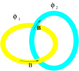
FIG. 1.: Two linked $B$ flux tubes with no twist in the field lines and with linking number ${\cal L}_{12}=+1$.

Within each filament, the ${\bf B}$-lines are unlinked curves which close on themselves after just one passage round the filament. The helicity $H$ of the two flux tubes has the same form as the pseudo-scalar quantity described in (5).

Adopting the coulomb gauge for ${\bf A}$ (i.e. $\nabla\cdot{\bf A}=0$), and imposing the further condition ${\bf A}=O(|r|^{-3})$ as $|r|\rightarrow\infty$, ${\bf A}$ is given by the Biot-Savart law:

$${\bf A}(r)=\frac{1}{4\pi}\int\frac{{\bf B}(r^{\prime})\times({\bf r}-{\bf r}^{\prime})}{|{\bf r}-{\bf r}^{\prime}|^{3}}dV^{\prime},$$ (6)

so that from (5),

$$H=\frac{1}{4\pi}\int\int\frac{{\bf B}(r)\times{\bf B}(r^{\prime})\cdot({\bf r}-{\bf r}^{\prime})}{|{\bf r}-{\bf r}^{\prime}|^{3}}dVdV^{\prime}.$$ (7)

Each tube may be built of many infinitely small flux tubes carrying fluxes $\delta\phi_{1}$ and $\delta\phi_{2}$. Replacing ${\bf B}dV$ by $\delta\phi\,d{\bf l}$: allowing for the fact that each flux filament is integrated over twice once as $r$ and once as $r^{\prime}$, we find that $\delta H=2\,{\cal L}_{12}\,\delta\phi_{1}\delta\phi_{2}$ with

$${\cal L}_{12}=\frac{1}{4\pi}\oint_{C_{1}}\oint_{C_{2}}\frac{(d{\bf l}\times d{\bf l}^{\prime})\cdot({\bf r}-{\bf r}^{\prime})}{|{\bf r}-{\bf r}^{\prime}|^{3}}$$ (8)

which is the Gauss formula for the linking of two curves. The sign of ${\cal L}_{12}$ depends on the relative orientations of the field in the two filaments (according to the right hand rule).

It is simple to obtain the total helicity of the two flux tubes. Each pair of filaments (one from each tube) make a contribution $2{\cal L}_{12}\,\delta\phi_{1}\delta\phi_{2}$ to the total helicity, so that summing over all such pairs, this is now given by

$$H=2\,{\cal L}_{12}\,\phi_{1}\phi_{2}.$$ (9)

Helicity has been shown to be an invariant for flows in which the divergence free field lines are frozen into the flow (Woltjer [24, 25] for a perfectly conducting fluid and Moffatt [6] for ideal barotropic flow). Combining this knowledge with (9), the interpretation of the invariant in terms of conservation of linkage of the (vortex/magnetic) field lines which are frozen in the fluid is immediate.

III Helicity of Global Cosmic Strings

States of a Higgs field containing a tangle of cosmic strings resemble a tangle of quantum vortex filaments which arise in quantum turbulent flow in superfluids. They are both described by a complex wave function $\psi=\rho e^{\imath\theta}$ and a winding number $N$. The phase $\theta$ changes by $2\pi N$ when one goes once around the filament or string axes. The curve $\rho=0$ defines the position of the strings and the passage from $\rho=0$ to the vacuum value of $\rho$ takes place over a certain lengthscale denoted by $r_{0}$. This lengthscale is very small in comparison with the strings lengths and distances between the strings, i.e. the strings are very thin.

Motivated by this resemblance Bekenstein [16] designed a helicity for cosmic strings in analogy with fluid helicity of a superfluid. We first review the original calculation [16] of the helicity of a tangle of strings, and then correct it for the left-out contribution of internal helicity.

A Constructing the helicity of global cosmic strings

In a superfluid the velocity is proportional to the gradient of the phase of the wave function; Bekenstein defines the vector

$${\bf v}=\Theta({\rho}^{2})\nabla\theta,$$ (10)

where $\Theta({\rho}^{2})$ is taken to be a function which rises rapidly from its value at a string axis $\Theta(0)=0$ to near its asymptotic value, $\Theta(\rho^{2}_{0})=1$, over an interval of $\rho^{2}$ which corresponds to a distance of order $r_{0}$. ${\bf v}$ is a kind of regularised velocity in that the singularity of $\nabla\theta$ on the axis is defused by the $\Theta$ function (far from the axis ${\bf v}$ will drop inversely with the distance from it as befits a vortex velocity field). We have

$$\nabla\times{\bf v}=\Delta({\rho}^{2})\nabla{\rho}^{2}\times\nabla\theta,$$ (11)

where $\Delta({\rho}^{2})$ is the derivative of $\Theta({\rho}^{2})$ with respect to ${\rho}^{2}$. $\Delta({\rho}^{2})$ has a rather sharp peak at a distance $\approx r_{0}$ from a string axis and the integral of $\Delta$ over all ${\rho}^{2}$ is unity.

The helicity of the field ${\bf v}$ is defined as

$$h=\int{\bf v}\cdot\nabla\times{\bf v}\,d^{3}r.$$ (12)

Unlike ordinary fluid helicity, this one vanishes. This is clear since the vectors ${\bf v}$ and $\nabla\times{\bf v}$ are perpendicular by construction. Nevertheless, string loops (and vortex rings) can link, and knot, and their linkage is correlated with other topological properties of the strings to be introduced later.

Throughout it is assumed that linked and knotted loops can occur over some periods with no intersections. Situations where there are intersecting strings are viewed as representing singular moments, not generic ones. (Simulations of the development of superfluid vortices [5] and global cosmic strings [21] confirm this assumption). Bekenstein develops from the zero helicity a quantitative relation between the linkage and other properties of the loops.

B Evaluation of global cosmic strings helicity

In order to evaluate the helicity explicitly for a tangle of cosmic string loops, it is convenient to rewrite (12) as a two-point functional of ${\bf v}$  (This is valid if the loops are confined to a finite region [16])

$$h=H[{\bf v}]=\int d^{3}r\int d^{3}r^{\prime}\,\frac{(\nabla\times{\bf v})\times(\nabla\times{\bf v})^{\prime}\cdot({\bf r}-{\bf r}^{\prime})}{4\pi|{\bf r}-{\bf r}^{\prime}|^{3}}.$$ (13)

We follow Bekenstein in the following discussion of the reduction of $H[{\bf v}]$, and the conclusions that may be drawn from it. For field configurations of size large compared to $r_{0}$, and where all the string axis are always well apart on scale $r_{0}$, $H$ receives a contribution only when each of ${\bf r}$ and ${\bf r}^{\prime}$ lies very close to a string axis. This stems from the fact that the $\Delta$ function in (11) confines the integrals to very near the axis. Hence, Bekenstein assumes $H$ is equivalent to a double line integral taken along the string axis. In addition the cross section of each loop is very little distorted by the presence of the other loops and nearby portions of itself and therefore is assumed to possess a line symmetry. Under these assumptions and a few manipulations Bekenstein concludes that

$$\int d^{3}r\,\nabla\times{\bf v}=2\pi|N|d{\bf s}$$ (14)

for the contribution of a little piece of string, where $d{\bf s}$ here is the vectorial line element along the piece of string considered.

Inserting (14) into (13) we obtain a double contribution to helicity from each pair of loops, because $d{\bf s}$ may progress through one loop (call it $\ell_{i}$) while $d{\bf s}^{\prime}$ does so through the other ($\ell_{j}$) and vice-versa. In addition we obtain a contribution from each string loop alone so that

$$H[{\bf v}]=\frac{1}{2}\sum_{i\neq j}2{\cal L}_{ij}(2\pi|N_{i}|)(2\pi|N_{j}|)+\sum_{i}{\cal W}_{i}(2\pi|N_{i}|)^{2}.$$ (15)

where

$${\cal L}_{ij}=\frac{1}{4\pi}\oint_{\ell_{i}}\oint_{\ell_{j}}\frac{d{\bf s}\times d{\bf s}^{\prime}\cdot({\bf r}-{\bf r}^{\prime})}{|{\bf r}-{\bf r}^{\prime}|^{3}}$$ (16)

is the Gauss linking number (8) of the two loops $\ell_{i}$ and $\ell_{j}$ and

$${\cal W}_{i}=\frac{1}{4\pi}\oint_{\ell_{i}}\oint_{\ell_{i}}\frac{d{\bf s}\times d{\bf s}^{\prime}\cdot({\bf r}-{\bf r}^{\prime})}{|{\bf r}-{\bf r}^{\prime}|^{3}}$$ (17)

is the writhing number of loop $i$ (Fuller [23]). While ${\cal L}_{ij}$ is a topological invariant of the linking of the string loops and must be an integer, ${\cal W}_{i}$ is not a topological invariant. It changes with the shape of the loop and can obtain any value. ${\cal W}_{i}$ measures the deviation of a loop from its plane; the writhe of a planar loop is zero.

When all loops are confined to a finite region, $H=h=0$, and (15) gives

$$0=(2\pi)^{2}\sum_{i\neq j}{\cal L}_{ij}|N_{i}||N_{j}|+(2\pi)^{2}\sum_{i}{\cal W}_{i}N_{i}^{2}.$$ (18)

We thus obtain a constraint connecting the linking of a collection of loops with their geometrical shapes. Particularly simple is the case of an isolated loop. Then ${\cal L}_{ij}=0$. For such a loop we must have ${\cal W}_{i}=0$ too. According to this result an isolated un-knotted loop must be a planar loop at any instant [16]. This is hard to accept since dynamically there seems to be no constraint on a loop accumulating a distortion continuously in an arbitrary direction. Furthermore simulations of the formation and evolution of cosmic strings [20, 21] show the formation of loops which are not planar! Similarly, according to (18) two loops linked once may never be planar since the contribution of their writhe to the helicity must cancel out the contribution from their linkage. This restriction is again hard to accept.

To obtain another constraint Bekenstein introduces the relation [22, 23]

$${\cal K}={\cal W}+{\cal C}.$$ (19)

${\cal K}$ measures the knotting of the curve and can jump by increments of $\pm 2$, and ${\cal C}$ is the contortion of the loop defined by ${\cal C}=(2\pi)^{-1}\oint\tau ds$ which integrates the torsion over the whole loop. Inserting ${\cal W}$ from (19) into (18) gives the following constraint connecting the contortion, knotting and linking of a collection of loops:

$$\sum_{i}{\cal C}_{i}N_{i}^{2}=\sum_{i\neq j}{\cal L}_{ij}|N_{i}N_{j}|+\sum_{i}{\cal K}_{i}N_{i}^{2}.$$ (20)

This relation says that the sum of contortions of a collection of unit winding number loops is quantized in integers [16]. This implies that the contortion of any single knot is quantized in integers: the knot cannot wiggle freely about, but is frozen in a configuration of integer contortion. This is a very strong constraint on the dynamics of such a configuration, and together with our previous observations, makes us suspect that the calculation has missed a term.

C Internal helicity

The first clue of the missing term was presented by Moffatt [4], who notes that close inspection of an expression of the form

$$H_{\ell_{i}}=\int_{\ell_{i}}d^{3}r\int_{\ell_{i}}d^{3}r^{\prime}\frac{(\nabla\times{\bf v})\times(\nabla\times{\bf v})^{\prime}\cdot({\bf r}-{\bf r}^{\prime})}{4\pi|{\bf r}-{\bf r}^{\prime}|^{3}},$$ (21)

integrated over a single flux loop $\ell_{i}$ (of an arbitrary divergence-free vector field), shows that the helicity in this limit has an additional contribution from pairs of points ${\bf r}$, ${\bf r}^{\prime}$ separated by a distance comparable to the cross-sectional span of the loop. In addition to the writhe ${\cal W}$ (17), which we introduced earlier as the sole contribution to helicity from a single loop, Moffatt conjectures that the close points contribute an extra term namely

$$H_{\ell_{i}}={\cal C}_{\ell_{i}}\phi^{2}$$ (22)

where ${\cal C}_{\ell_{i}}$ is the contortion of loop $i$ defined earlier, and $\phi$ is the flux of the loop. Actually it is easy to see that Bekenstein’s calculation in Sec. III B ignores the thickness of the string, i.e. the contribution from close pairs of points ${\bf r}$ and ${\bf r}^{\prime}$. Equation (14) reduces a volume integral to a line integral along the core of the string and thus treats the string as though it where infinitely thin. Moffatt speculates that the additional contribution, from close pairs of points ${\bf r}$ and ${\bf r}^{\prime}$, is related to the contortion so that the helicity will be a topological invariant of the loop, i.e., $H_{\ell_{i}}=({\cal W}_{\ell_{i}}+{\cal C}_{\ell_{i}})\phi^{2}={\cal K}_{\ell_{i}}\phi^{2}$ by (19). But, thinking this over we realize that the contortion is also just a property of the flux tube’s (string’s) axis and not of its internal structure hence we should expect a different term to appear.

Later Moffatt [7] explicitly calculated the helicity of a magnetohydrodynamic system of flux tubes to find that his earlier speculation was not exact, and that ${\cal K}$ is not a topological invariant after all since its value jumps discontinuously at inflexion points (points of zero curvature). In this later calculation Moffatt manipulates the magnetohydrodynamic equation of motion of a configuration of field lines moving with the flow. This calculation is much too complicated to carry over to the case of cosmic strings since the field equations for these are non-linear. Hence we will follow in the footsteps of Berger and Field [8] who also calculate the internal helicity due to the internal structure of a flux tube, but we will present a slightly different calculation, and a slightly different result. Berger and Field’s result was that $H=T\phi^{2}$ where $T$ is any real number, while we obtain the same result as Moffatt [7] with $H=n\phi^{2}$ and $n$, an integer, is the linking number of the field lines in the flux tube.

We first calculate exactly the contribution to the helicity of a single vortex loop $\ell$. First we consider the inner structure of the string to consist of nested toroidal vorticity surfaces (a peace of the loop is shown in Fig. 2). Then we may build up the string by increments of vorticity flux $d\phi$ composed of many thin flux tubes $\delta\phi$ that wind around the inner flux tube $\phi$ $n$ times.

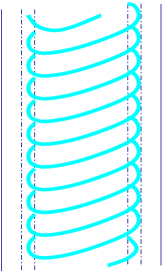
FIG. 2.: The linking of flux tubes inside a string.

The increment in helicity for each such flux tube $\delta\phi$ is $2n\phi\delta\phi$ where $n$ is the Gauss linking number of element $\delta\phi$ with $\phi$ (the inner flux tube). The increment in helicity for the whole of $d\phi$ is simply $2n\phi d\phi$. (The flux $d\phi$ simply counts the number of field lines intersecting the increment in the cross section of the string, and hence the number of field lines wrapped around the flux tube in the center.) We thus have according to (13)

$$H_{\ell} = \int_{\ell}d^{3}r\int_{\ell}d^{3}r^{\prime}\frac{(\nabla\times{\bf v})\times(\nabla\times{\bf v})^{\prime}\cdot({\bf r}-{\bf r}^{\prime})}{4\pi|{\bf r}-{\bf r}^{\prime}|^{3}}$$ (23)

$$= \int_{0}^{\phi}d\phi\,\phi\oint\oint\frac{(d{\bf l}\times d{\bf l}^{\prime})\cdot({\bf r}-{\bf r}^{\prime})}{4\pi|{\bf r}-{\bf r}^{\prime}|^{3}}=\int_{0}^{\phi}d\phi\,\phi\,2n$$ (24)

Where $d{\bf l}$ is along the axis of the string and $d{\bf l}^{\prime}$ is along one of the field lines in $\delta\phi$ wrapping $\phi$, and vice-versa. Finally, integrating over all the nested flux tubes

$$H_{\ell}=\frac{\phi^{2}}{2}2n=n(2\pi N)^{2},$$ (25)

where $N$ is the winding number of the cosmic string (the flux $\phi$ is easily calculated using the definition of ${\bf v}$, Stoke’s theorem and (1)).

Throughout this calculation we have assumed that $\delta\phi$ and $\phi$ have the same linking number as a single field line in $\delta\phi$ with the axis of the string. We have also assumed that all field lines have the same linking number with the axis of the string (and with each other). This is plausible for a continuous field. As we see, the internal helicity is due to the linking of the $\nabla\times{\bf v}$ field lines inside the string. This linking occurs when the field $\nabla\times{\bf v}$ is twisted: if the field lines do not link the internal helicity is zero.

We would now like to express the linking number of the field lines $n$ as a sum of ${\cal W}$ and some other term or terms, so that we may reconcile this calculation with Bekenstein’s result (15). The linking number $n$ of $\delta\phi$ with $\phi$ is equal to the linking number of a single field line in $\delta\phi$ with the axis of the string. Since these are two closed curves at a very short distance apart, the axis of the string can be treated as a curve in differential geometry, forming the edge of a ribbon whose other edge is traced by the field line.

This type of problem appears first to have been addressed by Călugăreanu [27, 28], who considered two neighboring closed curves $C$, $C^{*}$ forming the boundaries of a (possibly knotted) ribbon of small spanwise width $\epsilon$, and showed that for sufficiently small $\epsilon$ the linking number $n$ of $C$ and $C^{*}$ can be expressed in the form

$$n={\cal W}+{\cal C}+{\cal N},$$ (26)

where ${\cal W}$ and ${\cal C}$ are respectively the writhe and the contortion of $C$, and ${\cal N}$ is an integer representing the number of rotations of the unit spanwise vector $U$ on the ribbon relative to the Frenet pair (the unit normal and unit binormal) in one passage round $C$. (the contortion ${\cal C}$ actually measures the rotation round the curve of the Frenet pair itself.)

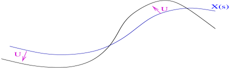
FIG. 3.: Two curves form the edges of a ribbon. $U$ is the unit spanwise vector of the ribbon and $X(s)$ is the curve of one of the edges of the ribbon

The Frenet pair has discontinuous behavior in going through a point of inflexion (zero curvature). As a result ${\cal C}$ and ${\cal N}$ are not well defined if $C$ has inflexion points. If $C$ is continuously deformed through an inflexional configuration, then ${\cal C}$ is discontinuous by $\pm 1$, but ${\cal N}$ is simultaneously discontinuous by an equal and opposite amount $\mp 1$, so that the sum ${\cal C}+{\cal N}$ does vary continuously through inflexion points [7]. This sum is known as the twist of the ribbon [22, 23, 29]

$${\cal T}={\cal C}+{\cal N}.$$ (27)

Thus, as we remarked earlier, ${\cal K}={\cal W}+{\cal C}$ is not a topological invariant while $n$ (26) is.

With the help of (26) and (27) we are now ready to complete the calculation of the helicity for a single (un- knotted) cosmic string loop $\ell$. We take $C$ above to be the string’s axis and $C^{*}$ to be along one of the field lines twisted around the axis. Then for the $i$-th loop

$$H_{\ell_{i}}=n_{i}\phi^{2}={\cal W}_{i}(2\pi N_{i})^{2}+{\cal T}_{i}(2\pi N_{i})^{2}.$$ (28)

Our final expression for the helicity of a tangle of cosmic string loops is therefore

$$H[{\bf v}]=\sum_{i\neq j}{\cal L}_{ij}(2\pi|N_{i}|)(2\pi|N_{j}|)+\sum_{i}{\cal W}_{i}(2\pi N_{i})^{2}+{\cal T}_{i}(2\pi N_{i})^{2}.$$ (29)

Contrast this (correct) result with (15). The twist ${\cal T}$ is the contribution from the close pairs of points ${\bf r}$ and ${\bf r^{\prime}}$ inside the string; it is not a property of the axes of the string alone, but rather of the internal structure of the field lines inside the string core.

IV New Constraints on String Configurations

In the previous sections we learned that helicity measures the linkage of the field lines of $\nabla\times\bf v$, and that the total helicity of global cosmic strings is zero whatever their configuration may be. These properties must put some constraint on the possible configurations of the strings. In this section we show that the knotting and external linkage of a cosmic string determines the internal structure of the field lines inside the string, and thus external and internal helicity cancel each other out so that the total helicity is zero. Since the field lines in a string must close on themselves, and their twist depends on external knotting and linking, we will get constraints on the possible configurations of string loops. These constraints are weaker than those proposed by Bekenstein, and are free from the latter’s paradoxical aspects.

A Determining internal linking from winding numbers of a string loop

Let us start by examining $\nabla\theta$ (the gradient of the phase) of the most simple configuration, a single loop. As we know the phase varies when one goes once around the string by $2\pi N$, where $N$ is the winding number of the string.

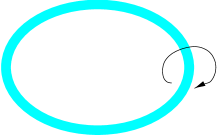
FIG. 4.: Sense of variation of the phase for an isolated cosmic string loop.

What happens if the phase varies along the string too? Because of periodicity this is only possible if

$$\oint\nabla\theta_{s}\cdot d{\bf s}=2\pi N^{\prime}$$ (30)

where $d{\bf s}$ is along the string axis. But in this case there will be another topological requirement. Because the phase varies by $2\pi N^{\prime}$ around the perimeter of the loop, for every surface spanning the loop there must be at least one place where the amplitude $\rho=0$ so that the field $\psi$ will be single-valued. This is actually the requirement that the loop be threaded by another $N^{\prime}$ unit winding-strings or a single string with winding number $N^{\prime}$. Hence an isolated loop must have $N^{\prime}=0$; for a totally symmetric loop $\nabla\theta$ will have only one component, in the direction around the string.

How does this affect the configuration of the field lines of $\nabla\times\bf v$ ? We recall that by definition (10), $\bf v$ is parallel to $\nabla\theta$ and $\nabla\times\bf v$ (11) is perpendicular to $\bf v$. Hence if $\bf v$ has a component only around the string, $\nabla\times\bf v$ will have a component only along the string, and its field lines will not be twisted or linked. Since linkage of the field lines is a topological property, it will not change for continuous deformation of the loop; therefore the field lines of any isolated loop with arbitrary shape will be unlinked. The immediate result is that the total helicity of any isolated loop with arbitrary shape is zero. This corrects Bekenstein’s conclusion (18) that an isolated loop must be a planar loop at any instant so that the helicity will be zero.

We next investigate a configuration of two linked loops $\ell_{1}$ and $\ell_{2}$ with winding numbers $N_{1}$ and $N_{2}$ respectively. We now have a component of $\nabla\theta$ in the direction along the strings too. The phase will vary around the perimeter of loop $\ell_{1}$ by $2\pi N_{2}$ and around the perimeter of $\ell_{2}$ by $2\pi N_{1}$ (Fig. 5). Now that $\nabla\theta$ has components along the string and around it, we must introduce a new concept, the chirality (handedness) of a string loop. A loop is right-handed (and has positive chirality) when the component of $\nabla\theta$ along the string is in the direction of the thumb of the right hand, whose fingers point along the component of $\nabla\theta$ around the string. If the component of $\nabla\theta$ along the string is in an opposite direction to the thumb, the loop is left-handed (and the chirality is negative).

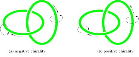
FIG. 5.: Two flat linked cosmic strings. For reasons of continuity the phase along the linked string must change by the same amount as the change in the phase around the other string. Only strings with the same chirality can link.

Along with the definition of chirality comes the definition of the sign of the directions along and around the string. We define the positive direction around the string to coincide with the direction of $\nabla\theta$ around it, and the positive direction along the string to coincide with the direction of the thumb of the right hand whose fingers follow the direction of $\nabla\theta$ around the string axis. In a right-handed (left-handed) string loop whose phase changes around the string by $2\pi N$ and along the string by $2\pi N^{\prime}$, $N$ and $N^{\prime}$ will have equal (opposite) signs. It is easy to see that two strings may link only if they have the same chirality; otherwise there would be a discontinuity in the phase.

What will be the structure of the $\nabla\times\bf v$ field lines in such a configuration? Now that $\nabla\theta$ has components in two directions, $\nabla\times\bf v$ will also have at least two components, one along the string and one around it. The field lines will be twisted and linked (Fig. 6).

In such a case we expect to have two contributions to helicity, a contribution from the external linkage of the string loops, and a contribution from the internal linkage of the field lines inside the strings. These two contributions must cancel each other so that this configuration may exist. The external helicity for such a configuration with ${\cal L}_{12}={\cal L}_{21}=\pm 1$ and winding numbers $N_{1}$ and $N_{2}$ is simply

$$H_{ext}={\cal L}_{12}(2\pi N_{1})(2\pi N_{2})+{\cal L}_{21}(2\pi N_{2})(2\pi N_{1})=\pm 2(2\pi N_{1})(2\pi N_{2}),$$ (31)

where the sign of ${\cal L}_{12}$ is determined by the relative direction of $\nabla\times\bf v$ along the perimeter of both loops. We will show below that ${\cal L}_{12}$ is positive for right-handed configurations and negative for left-handed ones.

But computing the internal helicity

$$H_{int}=n_{1}(2\pi N_{1})^{2}+n_{2}(2\pi N_{2})^{2}$$ (32)

is not straightforward. The internal helicity of magnetic flux tubes in a magnetohydrodynamic fluid or of vortices in an ordinary fluid is arbitrary since there is no restriction on the linking of the field lines inside the flux tube. In those systems the internal structure of the field lines is not determined by the topology of the flux tubes or vortex filaments and, therefore, the total helicity cannot be determined exactly from their configuration. By contrast we shall now show that the internal helicity of cosmic strings is solely determined by the winding numbers of the strings and their topological configuration, so that the total helicity for a configuration of linked vortices can be expressed as a function of their linkage and winding numbers alone.

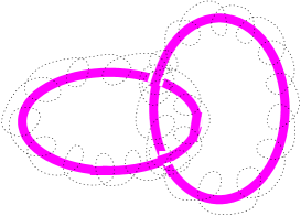
FIG. 6.: The twist in the vorticity field $\nabla\times\bf v$ for two linked strings. When strings are linked the phase must change along the string too. Hence $\nabla\theta$ will have a component along the string in addition to its component around the string. As a result $\nabla\times\bf v$ also has components along and around the string, and its field lines are twisted and link each other.

We now attempt to derive the internal linking number $n$, that measures the linkage of the field lines inside a cosmic string loop. The loop is characterized by winding numbers $N$ and $N^{\prime}$ around and along the perimeter of the loop respectively. Any (un-knotted) cosmic string loop may be deformed continuously into a planar circle loop, and the twist of the field lines inside it uniformly distributed, without changing the linking of the field lines. This is possible since the linking is a topological property of the field lines, and does not change by continuous deformations. It would further simplify our calculation if we could perform it in cylindrical symmetric coordinates, by virtually cutting the loop and standing it upright, such that it acquires cylindrical symmetry (Fig. 7). We may convince ourselves that this is possible since very close to the axis of the string the field lines have cylindrical symmetry around the string, and for reasons of continuity the linkage of the field lines cannot change as we move away from the string.

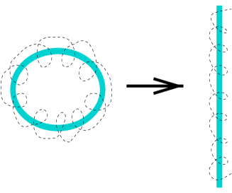
FIG. 7.: A string loop may be virtually cut open and straightened out without changing the linking of the field lines.

The linking number $n$ is simply the number of times $\nabla\times\bf v$ is wrapped around the $z$ axis (which coincides with the axis of the string). This must be an integer for the string to form a loop. The vectors $\bf v$ and $\nabla\times\bf v$ are computed in cylindrical symmetric coordinates $(r,\varphi,z)$ as follows: First

$${\bf v}=f(r)\nabla\theta,$$ (33)

where $\Theta({\rho}^{2})$ in (10) is taken to be $f(r)$, a function of $r$ only. The gradient of $\theta$ must obey

$$\oint\nabla\theta_{\varphi}\cdot rd\varphi=2\pi N\quad\textstyle{and}\quad\int_{0}^{L}\nabla\theta_{z}\cdot dz=2\pi N^{\prime},$$ (34)

where $L$ is the length of the string. Hence for uniformly distributed twist

$$\nabla\theta=\frac{N}{r}\hat{\varphi}+\frac{2\pi N^{\prime}}{L}\hat{z}.$$ (35)

The calculation of $\nabla\times\bf v$ gives

$$\nabla\times{\bf v}=f^{\prime}(r)\left(N\hat{z}-\frac{2\pi r}{L}N^{\prime}\hat{\varphi}\right).$$ (36)

We are interested in the number of times each field line encircles the $z$ axis. Often we associate flow lines with vector fields by imagining how a test particle would move if the vector field were its velocity field. Let us assume the field line traces out the trajectory of a point particle traveling with constant velocity during a period of time $t$. The velocity components of the particle are equal to the components of $\nabla\times\bf v$. The following simple equations must apply so that the field lines may reconnect when the string forms a loop

$$(\nabla\times{\bf v})_{z}\cdot t=L\quad\textstyle{and}\quad(\nabla\times{\bf v})_{\varphi}\cdot t=n\cdot 2\pi r.$$ (37)

By eliminating $t$ between the two equations and using $\nabla\times\bf v$ from (36) we obtain the result

$$n=-{N^{\prime}}/{N}.$$ (38)

Thus the internal linking number $n$ depends exclusively on the winding numbers of the loop.

To evaluate the total helicity for two linked un-knotted cosmic string loops, we first determine the sign of the Gauss linking number ${\cal L}_{12}$ for left-handed and right-handed configurations, which depends on the direction of $\nabla\times\bf v$ along the perimeter of both loops. By our definition above, the winding numbers around the axis of the string are always positive, since we have defined the positive direction around the string to coincide with the direction of $\nabla\theta$ around the axis of the string. Hence from (36) the component of $\nabla\times\bf v$ along the axis is always in the positive direction i.e. along the thumb of the right hand whose fingers follow the positive direction around the axis of the string. Fig. 8 makes it clear that a right-handed configuration will have ${\cal L}_{12}=+1$ and the left-handed configuration will have ${\cal L}_{12}=-1$.

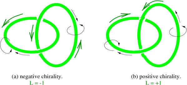
FIG. 8.: Right-handed linked strings have a positive Gauss linking number and left-handed linked strings have a negative Gauss linking number. The thick arrows represent the direction of $\nabla\times\bf v$ along the string while the thin ones represent $\bf v$. $\nabla\times\bf v$ is always in the positive direction along the axis of the string.

The sign of the internal linking number $n$ also depends on whether the configuration is left-handed or right-handed. As we explained earlier, in a right-handed configuration $N$ and $N^{\prime}$ have equal signs while in a left-handed configuration, they have opposite signs. Therefore, by (38) $n$ is negative for a right-handed pair and positive for a left-handed one. The signs of the external and internal linkages are opposite.

We are now able to write down the total helicity for a pair of linked strings. For two right-handed linked strings with winding numbers $N_{1}$ and $N_{2}$, we have $N_{1}^{\prime}=N_{2}$ and $N_{2}^{\prime}=N_{1}$ (since the axis of each loop encircles the other loop) and by (31) and (32) the total helicity is

$$H=2\cdot(2\pi N_{1})\cdot(2\pi N_{2})-\frac{N_{2}}{N_{1}}\cdot(2\pi{N_{1}})^{2}-\frac{N_{1}}{N_{2}}\cdot(2\pi{N_{2}})^{2}=0.$$ (39)

For two left-handed linked loops the total helicity is

$$H=-2\cdot(2\pi N_{1})\cdot(2\pi N_{2})+\frac{N_{2}}{N_{1}}\cdot(2\pi{N_{1}})^{2}+\frac{N_{1}}{N_{2}}\cdot(2\pi{N_{2}})^{2}=0.$$ (40)

The external and internal helicities thus cancel each other out without constraining the shapes of the loops.

We have thus removed the constraint on the geometrical shape of a single loop, a pair of linked loops or any other configuration. The contributions to helicity are purely topological. But (38) introduces a new topological constraint. The internal Gauss linking number $n$ of the field lines in the string must be an integer. Hence the winding number $N^{\prime}$ along the perimeter of the string is not free to take on just any value, i.e., a string loop with winding number $N$ cannot be linked arbitrarily with other loops. For the right handed pair of linked loops $\ell_{1}$ and $\ell_{2}$, for example, the internal linking number of $\ell_{1}$ is $n_{1}=-N_{2}/N_{1}$ and the internal linking number of $\ell_{2}$ is $n_{2}=-N_{1}/N_{2}$. Therefore we must have $N_{1}=N_{2}$ so that both $n_{1}$ and $n_{2}$ be integers. This means that only string loops with the same winding number may link once. In the next section we generalize this result to a generic configuration of linked un-knotted loops.

B Generalized topological constraint on configurations of un-knotted linked loops

Examining a couple more examples will help us formulate a more general result.

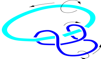
FIG. 9.: Two cosmic strings linked twice.

Fig. 9 depicts a right-handed cosmic string loop $\ell_{1}$ with winding number $N_{1}$ linked twice with a cosmic string loop $\ell_{2}$ with winding number $N_{2}$ such that their Gauss linking number is ${\cal L}_{12}=2$. As explained earlier the change in phase along the perimeter of a loop is determined by the winding numbers of the strings threading it. Since $\ell_{2}$ links $\ell_{1}$ twice the change in phase along $\ell_{1}$ is $2\pi\cdot 2N_{2}$ so that $N^{\prime}_{1}=2N_{2}$; correspondingly the phase along $\ell_{2}$ changes by $2\pi\cdot 2N_{1}$ so that $N^{\prime}_{2}=2N_{1}$. Hence the internal linking number of $\ell_{1}$ is $n_{1}=-2N_{2}/N_{1}$ and that of $\ell_{2}$ is $n_{2}=-2N_{1}/N_{2}$. Thus the values of $N_{2}$ must be restricted to the integers that divide $2N_{1}$ and are greater than or equal to $N1/2$. For a few examples see Table I, only such loops may link twice. The total helicity for this configuration is

$$H=2\cdot 2(2\pi N_{1})(2\pi N_{2})-\frac{2N_{2}}{N_{1}}\cdot(2\pi N_{1})^{2}-\frac{2N_{1}}{N_{2}}\cdot(2\pi N_{2})^{2}=0.$$ (41)

$\displaystyle\begin{array}[]{||l|l||}\hline\cr N_{1}&N_{2}\\ \hline\cr 1&1,2\\ 2&1,2,4\\ 3&3,6\\ 4&2,4,8\\ 5&5,10\\ 6&3,6,12\\ 7&7,14\\ 8&4,8,16\\ 9&9,18\\ 10&5,10,20\\ \hline\cr\end{array}$

TABLE I.: The only permissible values of $N_{2}$ for different values of $N_{1}$ for the configuration in Fig. 9.

Our second example in Fig. 10 depicts a left-handed string loop with winding number $N_{1}$ linked once with two other left-handed string loops, one with winding number $N_{2}$ and the other with winding number $N_{3}$.

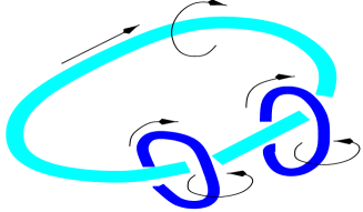
FIG. 10.: A cosmic string linked once with two others.

The external Gauss linking numbers are ${\cal L}_{12}=-1$ and ${\cal L}_{13}=-1$ and ${\cal L}_{23}=0$. The change in phase around the perimeter of the strings, and the internal linking numbers are determined by the same arguments as above, such that $n_{1}=(N_{2}+N_{3})/N_{1}$, $n_{2}=N_{1}/N_{2}$ and $n_{3}=N_{1}/N_{3}$. The total helicity will thus be

$$H = 2\cdot(-1)(2\pi N_{1})(2\pi N_{2})+2\cdot(-1)(2\pi N_{1})(2\pi N_{3})$$ (42)

$$+ \frac{(N_{2}+N_{3})}{N_{1}}\cdot(2\pi N_{1})^{2}+\frac{N_{1}}{N_{2}}\cdot(2\pi N_{2})^{2}+\frac{N_{1}}{N_{3}}\cdot(2\pi N_{3})^{2}=0$$ (43)

as we would expect.

By generalizing from these examples we see that the internal linking number $n_{i}$ for a loop $\ell_{i}$ linked with an arbitrary number of other loops is

$$n_{i}=\frac{-p\cdot\sum_{j\neq i}|{\cal L}_{ij}|N_{j}}{N_{i}},$$ (44)

where $p$ is equal to +1 for right handed loops and -1 for left handed ones. This equation is also a constraint on the winding numbers and the Gauss linking numbers of the loops linking $\ell_{i}$, since $n_{i}$ must come out an integer.

The total helicity of loops linked in an arbitrary manner thus vanishes:

$$H = 4\pi^{2}\left(p\cdot\sum_{i,j\neq i}|{\cal L}_{ij}|N_{i}N_{j}+\sum_{i}n_{i}N_{i}^{2}\right)$$ (45)

$$= 4\pi^{2}\left(p\cdot\sum_{i,j\neq i}|{\cal L}_{ij}|N_{i}N_{j}-\sum_{i}\cdot\frac{p\cdot\sum_{j\neq i}|{\cal L}_{ij}|N_{j}}{N_{i}}\cdot N_{i}^{2}\right)$$ (46)

$$= 4\pi^{2}\left(p\cdot\sum_{i,j\neq i}|{\cal L}_{ij}|N_{i}N_{j}-p\cdot\sum_{i}\sum_{i\neq j}|{\cal L}_{ij}|N_{j}N_{i}\right)=0.$$ (47)

V Electroweak Helicity of Local Cosmic Strings and Baryogenesis

Local cosmic strings are solutions to Lagrangians invariant under local gauge transformations. The simplest model for a local cosmic string is the Abelian Higgs model; it has $U(1)$ local symmetry. Nielsen and Olesen [30] found straight string (cylindrically symmetric) solutions to this model characterized by a magnetic field confined to the string’s core whose flux is quantized in proportion to the winding number $N$ of the string. Another important property of these strings is that they have finite energy per unit length (in contrast to the global strings) since the gauge field $A_{\mu}$ can cancel out the gradient of the phase at spatial infinity.

The Nielsen-Olesen string is actually a two dimensional vortex solution with energy density localized around a point in space, which can trivially be embedded into the extra dimension to produce an infinite string-like object whose energy density is localized along a line. By embedding the vortex along a closed curve, rather than a straight line, the ends of the string can be joined to produce a closed string of finite length. Thus we may have a configuration that is a tangle of such local cosmic strings which are both knotted and linked with each other. Since these strings have quantized magnetic flux tubes in their cores, we actually have a tangle of knotted and linked magnetic flux tubes, and each configuration may be characterized by a magnetic helicity quantifying the linking of the cosmic strings, and the internal linkage of the magnetic field lines inside each string.

In this section we refer to the result [17, 19, 31, 32] that the change in the electroweak magnetic helicity of a tangle of local cosmic strings, in the standard model, is related to baryon number violation. Previous works indicated a continuous change in baryon number. In contradiction to these works, We show here, by using our knowledge of the topological interpretation of helicity as the linking of field lines that, baryon number on local strings is quantized in this model.

A The term $I=\int d^{4}x\,F_{\mu\nu}\tilde{F}^{\mu\nu}$ for Nielsen-Olesen strings

Sato and Yahikozawa [18] scrutinize the geometrical and topological properties of the Abelian Higgs model with vortex strings by calculating the topological term $I$

$$I\equiv\int d^{4}x\,F_{\mu\nu}\tilde{F}^{\mu\nu},$$ (48)

which originates from the chiral anomaly, and is the CP violating $\theta$ term in the action. The definition of the dual is the following: $\tilde{F}^{\mu\nu}=\frac{1}{2}\epsilon^{\mu\nu\rho\sigma}F^{\rho\sigma}$. $I$ is evaluated for cases where all vortex strings are closed, with winding number $N=1$, and the number of the vortex strings is conserved i.e. vortex string reconnection does not occur. Using a topological formulation which they developed, and via a complicated calculation, Sato and Yahikozawa show that

$$I=-\frac{8\pi^{2}}{e^{2}}\Big{[}\sum_{i\neq j=1}^{n}{\cal L}_{ij}+\sum_{i=1}^{n}{\cal W}_{i}\Big{]}_{t=-\infty}^{t=+\infty}.$$ (49)

The first term is the linking number between each pair of strings and comes from the mutual interactions between different vortex strings. The second term is the writhing number; it comes from the self-interactions of each vortex string, and can vary with the shape of the string.

It is plain that the value of $I$ changes continuously with the shape of the strings as time elapses. Equation (49) strongly resembles Bekensteins result (15) for the helicity of global cosmic strings. We shall now show that $I$ is just the total change in time of the magnetic helicity of the Abelian Higgs model with local vortex strings, and hence equal to the change in the external and internal linking numbers of the magnetic field lines each weighed by the square of the quantized flux in the corresponding vortex.

By construction $F_{\mu\nu}\tilde{F}^{\mu\nu}=4{\bf E}\cdot{\bf B}$, so we may write

$$I=4\int d^{4}\,x{\bf E}\cdot{\bf B}.$$ (50)

Using Maxwell’s equations

$\displaystyle{\bf E}=-\frac{\partial{\bf A}}{\partial t}-\nabla\phi,\quad{\bf B}=\nabla\times{\bf A}$and

$\displaystyle\frac{\partial{\bf B}}{\partial t}=-\nabla\times{\bf{\bf E}},$and integration by parts,

$$\int d^{4}x\,{\bf E}\cdot{\bf B} = -\int d^{3}x{\bf A}\cdot{\bf B}\Big{|}_{t=-\infty}^{t=+\infty}+\int d^{4}\,x{\bf A}\cdot\frac{\partial{\bf B}}{\partial t}$$ (51)

$$= -\int d^{3}x{\bf A}\cdot{\bf B}\Big{|}_{t=-\infty}^{t=+\infty}-\int d^{4}x\,{\bf E}\cdot\nabla\times{\bf A}$$ (52)

where we have used the relation $\nabla\cdot({\bf E}\times{\bf A})={\bf A}\cdot(\nabla\times{\bf E})-{\bf E}\cdot(\nabla\times{\bf A})\,$and the assumption that all fields die off at spatial infinity. Our final result is thus

$$I=-2\int d^{3}\,x{\bf A}\cdot{\bf B}\Big{|}_{t=-\infty}^{t=+\infty}=-2\Delta H$$ (53)

where $H$ stands for the magnetic helicity.

As we already know, the magnetic helicity may be written as the sum of the external linkages of the flux tubes and the internal linkage of the field lines in each flux tube, times the square of the flux (29)

$$H=\sum_{i\neq j}{\cal L}_{ij}\cdot(\frac{2\pi}{e})^{2}+\sum_{i}{\cal W}_{i}\cdot(\frac{2\pi}{e})^{2}+\sum_{i}{\cal T}_{i}\cdot(\frac{2\pi}{e})^{2}.$$ (54)

The two terms ${\cal W}_{i}+{\cal T}_{i}$ add to $n_{i}$, the internal linking number (28), and the magnetic flux in a local string of unit winding number in this model is $2\pi/e$. Therefore, according to (53) and (54) the term $I$ is simply equal to

$$I=-\frac{8\pi^{2}}{e^{2}}\Big{[}\sum_{i\neq j}{\cal L}_{ij}+\sum_{i}{\cal W}_{i}+\sum_{i}{\cal T}_{i}\Big{]}_{t=-\infty}^{t=+\infty}.$$ (55)

Comparing this with (49) we see that Sato and Yahikozawa have missed out the twist term. This resulted from neglecting the internal structure of the vortex strings in their calculation. Our result is crucially different from theirs: according to their result the term $I$ may have a continuous range of values, while according to our result $I$ is quantized because $\Delta H$ is quantized by the internal and external linking numbers of the magnetic flux tubes threading the strings cores. This fact has an important physical consequence, as we shall see presently.

B The chiral anomaly and baryogenesis

The origin of the excess of matter over antimatter in our universe remains one of the fundamental problems. A widely discussed model [3, 35, 36, 37] is baryogenesis in the course of the broken symmetry electroweak transition, where the baryonic asymmetry is induced by the quantum chiral Adler-Bell-Jackiw anomaly [38, 39]. In models of fermions coupled to gauge fields, certain current-conservation laws are violated by this anomaly. The term $F_{\mu\nu}\tilde{F}^{\mu\nu}$ calculated on the background of the Nielsen-Olesen strings has been shown to cause violation of baryon number conservation via this anomaly.

The anomaly arises when a classical symmetry of the Lagrangian does not survive the process of quantization and regularization: the symmetry of the Lagrangian is not inherited by the effective action. An axial current that is conserved at the level of the classical equations of motion can thus acquire a nonzero divergence through one-loop diagrams that couple this current to a pair of gauge boson fields. The Feynman diagram that contains this anomalous contribution is a triangle diagram with the axial current and the two gauge currents at its vertices. Left and right handed fermions contribute terms with opposite signs to the anomaly; however, in chiral theories in which the gauge bosons do not couple equally to right- and left-handed species, the sum of these terms can give a non-zero contribution. In theories such as QED or QCD in which the gauge bosons couple equally to right- and left-handed fermions, the anomalies automatically cancel.

Within the standard model of weak interactions (the Glashow-Weinberg-Salam $SU(2)\times U(1)$ invariant theory), the requirement from experiment that weak interaction currents are left-handed forces us to choose a chiral gauge coupling. The coupling of the $W$ boson to quarks and leptons can be derived by assigning the left-handed components of quarks and leptons to doublets of an $SU(2)$ gauge symmetry, and then identifying the $W$ bosons as gauge fields that couple to this $SU(2)$ group, while making the right-handed fermions singlets under this group. The restriction of the symmetry to left-handed fields leads to the helicity structure of the weak interactions effective Lagrangian, and thus causes the chiral anomaly of the baryon current to arise. The baryon number current in this model is $j^{\mu}_{B}=\overline{Q}\gamma^{\mu}Q$ and the anomalous baryonic current conservation equation is

$$\partial_{\mu}j^{\mu}_{B}=\frac{N_{F}}{32\pi^{2}}(-g^{2}W^{a}_{\mu\nu}\tilde{W}^{a\mu\nu}+g^{\prime 2}Y_{\mu\nu}\tilde{Y}^{\mu\nu}),$$ (56)

where $W^{a}_{\mu\nu}$ and $Y_{\mu\nu}$ are the field strengths for the three $SU(2)$ and one $U(1)$ gauge fields $W^{a}_{\mu}$ ($a=1,2,3$) and $Y_{\mu}$ respectively, and $g$ and $g^{\prime}$ are their charges. $N_{F}$ is the number of quark families.

The baryon number current can be integrated to yield the change in the baryon number between two different times, if we assume that the baryonic flux through the surface of the three-volume of interest vanishes:

$$Q_{B} = \int d^{3}x\,j^{0}$$ (57)

$$\Delta Q_{B} = \int dt\,\partial_{0}Q_{B}=\int d^{4}x\,\partial_{0}j^{0}_{B}=\int d^{4}x\,\partial_{\mu}j^{\mu}_{B}.$$ (58)

Equations (56) and (58) relate the change in the baryon number to terms of the form $\int d^{4}x\,F_{\mu\nu}\tilde{F}^{\mu\nu}$ which we calculated in the previous section for an abelian model on the background of Nielsen-Olesen vortices. This term was found to be related to the change in the sum of the linking of the strings from their initial to final configurations (55). This leads us to an exciting idea [17, 31]: if chiral fermions are coupled to electroweak vortices, baryon number may be violated because of the anomaly as vortices link and de-link. For this to happen there must be a stable string solution in this model, and the change in the baryon number must be related to the helicity of an electroweak field whose flux is confined to the string.

It is generally believed that the standard electroweak model is free from topological defects. The reason is that the first homotopy group of

$\displaystyle M=G/H=\big{(}SU(2)_{L}\times U(1)\big{)}/U(1)_{em}$can be shown to be trivial i.e. $\Pi_{1}(M)=0$ [40, 41]. However, this does not mean that the model is free from non-topological defects. It has been shown by Manton [42] that the configuration space of classical bosonic Weinberg-Salam theory has a non-contractible loop. Hence an unstable, static, finite-energy solution of the field equations can exist. Vachaspati [43, 44] showed that exact vortex solutions exist, which are stable to small perturbations for large values of the Weinberg angle $\theta_{W}$ and small values of the Higgs boson mass. This expectation has been confirmed by the numerical results of James, Perivolaropoulos and Vachaspati [46].

Defining

$$Z_{\mu} = \cos\theta_{W}W_{\mu}^{3}-\sin\theta_{W}Y_{\mu}$$ (59)

$$A_{\mu} = \sin\theta_{W}W_{\mu}^{3}+\cos\theta_{W}Y_{\mu},$$ (60)

where $\tan\theta_{W}=g^{\prime}/g$, the static vortex solution that extremizes the energy functional was found to be:

$$\phi=f_{NO}(r)e^{im\theta}\left(\begin{array}[]{c}0\\ 1\end{array}\right),\quad Z_{\mu}={A_{\mu}}_{NO},$$ (61)

and

$$A_{\mu}=0=W_{\mu}^{a}(a=1,2).$$ (62)

The subscript $NO$ on the functions $f$ and $A_{\mu}$ means that they are identical to the corresponding functions found by Nielsen and Olesen for the usual Abelian-Higgs string. In other words, the Weinberg-Salam theory has a vortex solution which is simply the $NO$ vortex of the Abelian Higgs model embedded in the non-Abelian theory. Substituting this solution into (56) we have

$$\partial_{\mu}j^{\mu}_{B}=\frac{N_{F}\alpha^{2}}{32\pi^{2}}\cos 2\theta_{W}Z_{\mu\nu}\tilde{Z}^{\mu\nu}$$ (63)

where $\alpha=g^{\prime}\sin\theta_{W}+g\cos\theta_{W}$ and $\alpha^{2}=g^{2}+g^{\prime 2}$.

The change in the baryon number is now

$$\Delta Q_{B}=\frac{N_{F}\alpha^{2}}{16\pi^{2}}q\Delta\int d^{3}x\,{\bf Z}\cdot\nabla\times{\bf Z}$$ (64)

via equations (58), (63) and (53) and with $q=\cos 2\theta_{W}$ playing the role of baryon number charge. We see that the change in the baryon number is proportional to the change in the ${\bf Z}$ field’s helicity. For a configuration of tangled strings with arbitrary winding numbers $N_{i}$

$$\Delta Q_{B}=\frac{N_{F}\alpha^{2}}{16\pi^{2}}q\Delta\left(\sum_{i\neq j}{\cal L}_{ij}N_{i}N_{j}+\sum_{i}n_{i}N_{i}^{2}\right)\cdot\left(\frac{4\pi}{\alpha}\right)^{2}$$ (65)

where the flux of each vortex is $4\pi N_{i}/\alpha$. The final result for a configuration of strings with unit winding number is

$$\Delta Q_{B}=N_{F}q\Delta\left(\sum_{i\neq j}{\cal L}_{ij}+\sum_{i}n_{i}\right)$$ (66)

and baryon number is quantized.

VI Summary

Earlier works failed to fully implement the topological interpretation of helicity as the measure of the linkage of field lines of the divergence free field. Since field lines may be twisted and linked inside a vortex core, the inner structure of the field inside the core may not be ignored when calculating helicity terms. Neglecting internal helicity had led to peculiar results: unacceptable constraints on string configurations and continuous violation of baryon number. Once we add the contribution from the internal structure of the strings, we find new constraints on the configurations of linked global cosmic strings, which are physically more pleasing, and we also find that, the baryon number is quantized as we would expect.

Our work is another demonstration of the fact that helicity counts the linkage of the divergence free field lines. We explain how there is no contradiction between the fact that helicity counts the linkage of field lines, and that the total helicity of any configuration of knotted linked loops always manages to vanish. The vector $\mathbf{v}$ (10) constructed for the purpose of obtaining a helicity term for global cosmic strings is proportional to $\nabla\theta$. Hence it is perpendicular to $\nabla\times\mathbf{v}$ (11) and the helicity must vanish. On the other hand the helicity counts the linkage of field lines of $\nabla\times\mathbf{v}$, and these lines must have external and internal linkages for linked configurations of cosmic string loops. What we have discovered is that the field lines arrange themselves in such a manner that the external and internal helicities exactly cancel each other. The field lines inside a string may not link in an arbitrary manner, their linkage is constrained by the topological configuration of the string and by its linking relations to other strings. Further, we have discovered a constraint on the permitted configurations of un-knotted linked loops, in the form of (44) which must produce integer values. This constraint results from the combination of the topological character of helicity integrals with the topological nature of cosmic strings as topological defects.

In this work we confined ourselves to the problem of un-knotted linked loops. The problem of knotted configurations is far more complicated since it is hard to separate the external contribution to helicity (depending on the topology of the knot) from the internal contribution depending on the twist of the field lines inside the knot. Moffatt [7] proposed a method for calculating the external helicity, but it turns out that for some knotted configurations this method is ambiguous (it may be that it works only for chiral knots, i.e. knots that are not isotopic to their mirror images). Hence, we leave the treatment of knots to later work.

For local cosmic strings in the Standard Model, the change in the helicity of the electroweak magnetic field confined to the strings core is related to the change in baryon number over a period of time (64). Thus, baryon number conservation is violated as cosmic strings link and de-link. The idea that violation of baryon number may be related to the change in the linking of electroweak strings has been developed by Cohen and Manohar [31], Vachaspati and Field [17] and Garriga and Vachapati [32]. However, they neglected the contribution of the writhe of the strings to helicity. Sato [19] adds the writhe term, but misses out the twist term. This led to his conclusion that baryon number conservation is violated as vortices change their shape, which implies that baryon number may change continuously and, therefore, is not quantized. Only by including both the writhe and the twist terms, which together give the internal linkage of the field lines, do we recover a quantized baryon number!

Charge quantization has previously been related to flux quantization. It was suggested by Dirac in 1931 [47] to explain the quantization of the electric charge. This idea was developed further by Jehle [48]. In general, quantization of charges is not a direct consequence of standard (non-GUT) field theories. Particularly, the quantization of electric charge has no widely accepted explanation within the Standard Model. During the last decade it has been suggested [49] that the electric charges can be heavily constrained within the framework of the Standard Model. This is achieved partly by constraints related to the classical structure of the theory (such as the requirement that the Lagrangian be gauge-invariant), and from the cancelation of anomalies, at the quantum level. The novel idea in this work is that quantization of the baryon number may arise from the topological nature of helicity integrals calculated on the background of local cosmic strings and from the flux quantization in the strings.

REFERENCES

- [1] L. Onsager, Nuovo Cim. 6, Suppl. 2, 246 (1949).
- [2] R.P. Feynman, in: Progress in low temperature physics, Vol. 1, ed. C.J. Gorter (North-Holland, Amsterdam, 1955).
- [3] A. Vilenkin, and E..P.S. Shellard, in: Cosmic strings and other topological defects, (Cambridge U.P., Cambridge, 1994)
- [4] H.K. Moffatt, [1981], J. Fluid Mech. 106, 27 (1955).
- [5] R.J. Donnelly and C.E. Swanson, J. Fluid Mech. 173, 387 (1986); K.W. Schwartz, Phys. Rev. B 38, 2398 (1988).
- [6] H.K. Moffat, J. Fluid Mech. 35, 117 (1969).
- [7] H.K. Moffatt and R.L. Ricca, Proc. R. Soc. Lond. A 439, 411 (1992).
- [8] M.A. Berger and G.B. Field, J. Fluid. Mech. 147, 133 (1984).
- [9] V.I. Arnol’d, (in Russian), Proc. Summer School in Differential Equations, Ereran, Armenian SSR Acad. Sci. (1974). (Trans. in Sel. Math. Sov. 5, 327 (1986).)
- [10] E.A. Kuznetsov and A.V. Mikhailov, Phys. Lett. A 77, 37 (1980).
- [11] H. Hopf, Math. Annalen 104, 637 (1931).
- [12] J.H.C. Whitehead, Proc. N. A. S. 33, 117 (1947).
- [13] R.L. Davis and E.P.S. Shellard, Phys. Rev. Lett. 63, 2021 (1989).
- [14] V.L. Ginzburg, and L.P. Pitaevskii, Zh. Eksp. Teor. Fiz. 24, 1240 (1958). (Sov. Phys. JETP 7, 858 (1958)).
- [15] T.W.B. Kibble, J. Phys. A9, 1387 (1976).
- [16] J.D. Bekenstein, Phys. Lett. B 282, 44 (1992).
- [17] T. Vachaspati and G.B. Field, Phys. Rev. Lett. 73, 373 (1994).
- [18] M. Sato, and S. Yahikozawa, Nucl. Phys. B436, 100 (1995).
- [19] M. Sato, Shapes of cosmic strings and baryon number violation, hep-ph/9508375.
- [20] T. Vachaspati and A. Vilenkin, Phys. Rev. D 30, 2036 (1984).
- [21] E.P.S. Shellard and B. Allen, in: The formation and evolution of cosmic strings, eds. G. Gibbons, S.W. Hawking and T. Vachaspati (Cambridge U.P., Cambridge, 1990).
- [22] J.H. White, Am. J. Maths 91, 693 (1969).
- [23] F.B. Fuller, Proc. Natl. Acad. Sci. USA 68, 815 (1971).
- [24] L. Woltjer, Proc. Nat. Acad. Sci. U.S.A. 44, 489 (1958).
- [25] L. Woltjer, Proc. Nat. Acad. Sci. U.S.A. 44, 833 (1958).
- [26] J.J. Moreau, Séminaire d’Analyse convexe montpellier, Exposé no. 7 (1977).
- [27] G. Călugăreanu, Rev. Math. Pures Appl. 4, 5 (1959).
- [28] G. Călugăreanu, Czechoslovak. Math. J. 11, 588 (1961).
- [29] F.B. Fuller, Proc. Natl. Acad. Sci. USA 75, 3557 (1978).
- [30] H.B. Nielsen and P. Olesen, Nucl. Phys. B61, 45 (1973).
- [31] A.G. Cohen, and A.V. Manohar, Phys. Lett. B265, 406 (1991).
- [32] J. Garriga, and T. Vachaspati, Nucl. Phys. B438, 161 (1995).
- [33] S. Weinberg, The quantum theory of fields, (Cambridge U.P., Cambridge, 1996).
- [34] M.E. Peskin and D.V. Schroeder, An introduction to Quantum Field Theory, (Addison-Wesley, New York, 1995).
- [35] A.D. Dolgov, Rep. Prog. Phys. 222, 309 (1992).
- [36] N. Turok, in: Formation and interaction of topological defects, p.283, eds. A.C. Davis and R. Brandenberger (Plenum Press, New York, 1995).
- [37] M.B. Hindmarsh and T.W.B. Kibble, Rep. Prog. Phys. 58, 477 (1995).
- [38] S.L. Adler, Phys. Rev. 177, 2426 (1969).
- [39] J.S Bell and R. Jackiw, Nuovo Cim. 60A, 47 (1969).
- [40] S. Weinberg, Phys. Rev. Lett. 19, 1264 (1967).
- [41] A. Salam, Elementary Particle Theory, ed. N. Svarthholm, (Almquist and Forlag, Stockholm, 1968).
- [42] N.S. Manton, Phys. Rev. D 28, 2019 (1983).
- [43] T. Vachaspati, Phys. Rev. Lett. 68, 1977 (1992).
- [44] T. Vachaspati, Nucl. Phys. B397, 648 (1993).
- [45] Y. Nambu, Nucl. Phys. B130, 505 (1977).
- [46] M. James, L. Perivolaropoulos and T. Vachaspati, Nucl. Phys. B395, 534 (1993).
- [47] P.A.M. Dirac, Proc. Roy. Soc. (London) A133, 60 (1931).
- [48] H. Jehle, Phys. Rev. D 3, 306 (1971).
- [49] R. Foot, H. Lew and R.R. Volkas, J. Phys. G 19, 361 (1993).