Hawking radiation on a falling lattice

Abstract

Scalar field theory on a lattice falling freely into a 1+1 dimensional black hole is studied using both WKB and numerical approaches. The outgoing modes are shown to arise from incoming modes by a process analogous to a Bloch oscillation, with an admixture of negative frequency modes corresponding to the Hawking radiation. Numerical calculations show that the Hawking effect is reproduced to within 0.5% on a lattice whose proper spacing where the wavepacket turns around at the horizon is $\sim 0.08$ in units where the surface gravity is 1.

I INTRODUCTION

If nothing can emerge from a black hole then where does the Hawking radiation come from? Relativistic field theory tells us that it comes from a trans-Planckian reservoir of outgoing modes at the horizon[1]. The existence of such a trans-Planckian reservoir is doubtful on general physical grounds. It is the cause of the divergences in quantum field theory which are expected to be removed in a quantum theory of gravity, and in particular it would seem to imply an infinite black hole entropy unless canceled by an infinite negative “bare entropy”.

String theory has produced an account of the Hawking radiation and black hole entropy which requires no trans-Planckian reservoir, however in that picture instead of a black hole one has a stringy object in flat spacetime that arises from a black hole as the string coupling constant tends to zero[2]. Thus gravitational redshift plays no role in the string calculations and nothing is learned about the origin of the outgoing modes in a black hole spacetime. If we could follow the theory as the string coupling becomes strong we would presumably learn how it is that string theory produces the outgoing black hole modes.

Absent a quantum gravity description of the Hawking process, Unruh invented a fluid analog of a black hole[3] in which an inhomogeneous flow exceeds the long wavelength speed of sound creating a sonic horizon (see also [4, 5]). Quantizing the sound field Unruh argued that the horizon would radiate thermal phonons, in analogy with the Hawking effect, at a temperature given by $\hbar/2\pi$ times the gradient of the flow velocity at the horizon. Since the sound field has an atomic cutoff, and the physics of the fluid is completely understood in principle, the fluid model may provide a source of insight into the Hawking process.

The atomic cutoff produces dispersion of sound waves leading to subsonic propagation at high frequencies. It turns out that this dispersion is all that is needed to obviate the need for a trans-Bohrian reservoir. In the linearized theory, an outgoing short wavelength mode can be dragged in by the fluid flow and redshifted enough so that its increased group velocity overcomes the flow and it escapes to infinity. Investigations of a number of linear field theory models[6, 7, 8, 9, 10, 11] and lattice models[12] incorporating such high frequency dispersion have demonstrated this mechanism of “mode conversion” and have shown that the Hawking radiation is recovered. The dispersion in these models is not locally Lorentz-invariant since a frame is picked out in which to specify which frequencies are “high”. In the fluid model this is the local rest frame of the fluid. A real black hole also defines a preferred frame but it does so in a non-local way. Perhaps quantum gravity produces a dispersion effect related to this non-local notion of a preferred frame, or perhaps microphysics is just not locally Lorentz invariant. In any case, it seems worthwhile to understand the mechanism of the outgoing modes and Hawking radiation in these models for the hints it may provide about a correct quantum gravity account.

In [12] a falling lattice model was introduced to address the “stationarity puzzle”[17, 8]: how can a low frequency outgoing mode arise from a high frequency ingoing mode when it propagates only in a stationary background spacetime and hence has a conserved Killing frequency? In the continuum based dispersive models there is no satisfactory resolution of this puzzle. As the outgoing modes are traced backwards in time their incoming progenitors are squeezed into the short distance regime of the model which is not physically sensible.

A lattice provides a simple model for imposing a physically sensible short distance cutoff. It might seem at first that the most natural choice would be to preserve the time translation symmetry of the spacetime with a static lattice whose points follow accelerated worldlines. On a static lattice, however, the Killing frequency is conserved, so outgoing modes arise from ingoing modes with the same frequency, and there is no Hawking radiation. The in-vacuum therefore evolves to a singular state at the horizon. If the lattice points are instead freely falling, a discrete remnant of time translation symmetry can still be preserved. On such a lattice there is still a frequency conservation law, and the unsatisfactory resolution of the stationarity puzzle is that the lattice spacing in this case goes to zero at infinity (if the lattice points are asymptotically at rest)[12].

If we insist that the lattice spacing asymptotically approaches a fixed constant and that the lattice points are at rest at infinity, we find a fascinating resolution of the stationarity puzzle[12]: the lattice cannot have even a discrete time translation symmetry, since there is a gradual spreading of the lattice points as they fall toward the horizon. The timescale of this spreading is of order $1/\kappa$ where $\kappa$ is the surface gravity. This time dependence of the lattice is invisible to long wavelength modes which sense only the stationary background metric of the black hole, but it is quite apparent to modes with wavelengths of order the lattice spacing. On such a lattice the long wavelength outgoing modes come from short wavelength ingoing modes which start out with a high (lattice scale) Killing frequency which is exponentially redshifted as the wavepacket propagates to the horizon and turns around.

This behavior of wavepackets in the (time-dependent) falling lattice model was determined in [12] with the help of the WKB approximation in which the frequency is used as a Hamiltonian to solve for the wavepacket trajectory. It was also argued that, since the time dependence of the lattice is adiabatic for those modes with wavelength short enough to know they are on a lattice, these modes will remain unexcited on their way to the horizon and the ground state condition for the Hawking effect will be met. However, since the wavelength is of order the lattice spacing and the wavepacket can vary wildly on the lattice near the horizon, it is not obvious that the WKB approximation is reliable nor that the adiabatic argument really applies.

The primary motivation for the work reported here was to check the WKB and adiabatic assumptions by carrying out the exact calculation numerically using the lattice wave equation. We found that indeed the field behaves this way, and the Hawking radiation is recovered to within half a percent for a lattice spacing $\delta=0.002/\kappa$ which corresponds to a proper spacing $\sim 0.08/\kappa$ where the wavepacket turns around at the horizon. We also studied the deviations from the Hawking effect that arise as $\kappa\delta$ is increased, and our simulations reveal an interesting picture of how the wavepackets turn around at the horizon.

The precise choice of worldlines for the lattice points should not be important to the leading order Hawking effect as long as the ground state evolves adiabatically in the lattice theory. Our numerical results are consistent with this expectation, in that the particular worldlines depend on the lattice spacing yet the results converge to the continuum as the lattice spacing is decreased. Moreover it was shown recently[10], in a continuum model with high frequency dispersion, that when the preferred frame is changed from the free-fall frame of the black hole to that of a conformally related metric there is no leading order change in the Hawking radiation unless the acceleration of the preferred frame is very large. Presumably all that matters is that the preferred world lines flow smoothly across the horizon. From a fundamental point of view, if there really is a cutoff in some preferred frame, it is plausible that this frame would coincide with the cosmic rest frame and would fall across the event horizons of any black holes that form by collapse.

The remainder of this paper is organized as follows. In Section II the falling lattice model is set up, in Section III some results of the WKB method are shown, illustrating the frequency shift and the mode conversion at the horizon, and the role of the negative frequency branch is explained. In Section IV the results of the full numerical evolution are presented, and Section V contains a discussion or the results and directions for further work. The Appendix describes the finite differencing of the time derivates used in the numerical calculations.

We use units with $\hbar=c=\kappa=1$, where $\kappa$ is the surface gravity.

II FALLING LATTICE MODEL

In this section we set up the field theory on a lattice falling into a black hole in two spacetime dimensions.

A Black hole spacetime

We assume the spacetime metric is static, so[18] coordinates can be chosen (at least locally) such that the line element takes the form

$$ds^{2}=dt^{2}-\bigl{(}dx-v(x)dt\bigr{)}^{2}.$$ (1)

In these coordinates the Killing vector is given by

$$\chi=\partial_{t},$$ (2)

with squared norm

$$\chi^{2}=1-v^{2}(x).$$ (3)

For $v(x)$ we choose

$$v(x)=-\frac{v_{\rm max}}{\cosh(\beta x)},$$ (4)

where $v_{\rm max}$ and $\beta$ are positive constants. As $|x|\rightarrow+\infty$, $v(x)$ vanishes, so the line element becomes that of Minkowski spacetime. Provided $v_{\rm max}>1$ there is an ergoregion centered on $x=0$ in which the Killing vector is spacelike, and the boundaries of this region are black and white hole horizons at

$$x_{H}=\pm\beta^{-1}\cosh^{-1}(v_{\rm max}).$$ (5)

The surface gravity of the horizons is given by

$$\kappa=v^{\prime}(x_{H})=\beta\sqrt{1-v_{\rm max}^{-2}}.$$ (6)

The surface gravity sets the length scale for our spacetime, and we will keep it fixed. Hence it will be useful to employ units for which $\kappa=1$.

We now introduce a freely falling “Gaussian” coordinate $z$ which will be discretized to define a falling lattice. The worldlines with $dx=v(x)dt$ are geodesics of the metric (1) with proper time $t$, at rest as $|x|\rightarrow\infty$, and they are orthogonal to the surfaces of constant $t$. On these curves the quantity $t-\int dx/v$ is constant, so if $z$ is constant on these curves we must have $W(z(x,t))=t-\int dx/v$ for some function $W$. We choose this function so that $z=x$ at $t=0$, which implies that $W(z)=-\int^{z}dx/v=\sinh(\beta z)/\beta v_{\rm max}$, hence

$$\sinh(\beta z)=\sinh(\beta x)+\beta v_{\rm max}t.$$ (7)

In terms of $z$, the line element (1) takes the form

$$ds^{2}=dt^{2}-a^{2}(z,t)\,dz^{2},$$ (8)

with

$$a(z,t)=\frac{\cosh(\beta z)}{\sqrt{1+(\sinh(\beta z)-\beta v_{\rm max}t)^{2}}}.$$ (9)

We call $a(z,t)$ the “scale factor”, even though it depends on $z$ as well as $t$. It can also be expressed as

$$a(z,t)=\frac{v(x(z,t))}{v(z)}.$$ (10)

In $(t,z)$ coordinates the Killing vector (2) is given by

$$\chi=\partial_{t}-v(z)\partial_{z}=\partial_{t}-\frac{v(x(z,t))}{a(z,t)}\partial_{z}.$$ (11)

The scale factor is unity at $t=0$, and outside the black hole it grows towards the future. It is important to know how rapidly the scale factor is changing in time, since in the lattice theory that time dependence is not merely a coordinate effect and can therefore excite the quantum field. At the horizon the scale factor takes the value

$$a(z_{H},t)=\sqrt{1+2\kappa t+\kappa^{2}t^{2}/(1-v_{\rm max}^{-2})},$$ (12)

so $a(z_{H},t)\sim\kappa t$ for $\kappa t\;\raisebox{-3.44444pt}{$\stackrel{{\scriptstyle\textstyle>}}{{\sim}}$}\;1$. Thus the fractional rate of change $\partial_{t}a/a$ is of order $\kappa$. In general, we have

$$\partial_{t}a/a=\frac{\beta v_{\rm max}\sinh(\beta x)}{\cosh^{2}(\beta x)}$$ (13)

whose maximum outside the horizon ($\cosh(\beta x)>v_{\rm max}$) is $\kappa$ (at the horizon) if $v_{\rm max}\geq\sqrt{2}$ and $\kappa v_{\rm max}^{2}/2\sqrt{v_{\rm max}^{2}-1}$ if $v_{\rm max}\leq\sqrt{2}$. Thus $|\partial_{t}a/a|\;\raisebox{-3.44444pt}{$\stackrel{{\scriptstyle\textstyle<}}{{\sim}}$}\;O(\kappa)$ everywhere outside the horizon as long as $v_{\rm max}>1$ is not too close to unity.

B Lattice

The lattice is defined by discretizing the $z$ coordinate with spacing $\Delta z=\delta$. That is, we have only the discrete values $z_{m}=m\delta$. We will consider values of $\kappa\delta$ which range from 0.002 to 0.128. To give a feeling for the lattice we plot in Fig. 1 the $(t,x)$ coordinates of lattice point worldlines at intervals of 50 lattice points.

FIG. 1.: Every 50th lattice point, $t$ vs. $x$, for the case $\delta=0.004$ and $v_{\rm max}=\sqrt{2}$. In the black region of the plot the points are too close to resolve. The horizon is at $x\simeq 0.6$.

Since $dx=a(z,t)dz$ at constant $t$, the separation $\Delta x$ of the lattice points in Fig. 1 gives a direct representation of the scale factor. The proper lattice spacing is given by $a(z,t)\delta$ which, according to (12), grows approximately linearly with time at the horizon.

Note that there is a region where the lattice spacing becomes very small. This happens because we chose the spacing to be uniform at $t=0$. If the points did not bunch up outside the black hole before $t=0$, they could not wind up equally spaced at $t=0$, since they are all on unit energy free-fall trajectories. (The line element is symmetric under $(t,x)\rightarrow(-t,-x)$, so the points bunch up also outside the white hole horizon after $t=0$.)

To get a better idea of how sparse the lattice is near the horizon at the turning point of a typical wavepacket, we plot in Fig. 2 the velocity function $v$ (4) for every lattice point near the horizon at time $t=27$, for the case $v_{\rm max}=\sqrt{2}$ and $\kappa\delta=0.004$. In this case there are only 6 points in the region between $v(x)=0.5$ and the horizon, and the proper spacing at the horizon is $\sim\sqrt{2}\kappa\delta t\sim 0.15/\kappa$.

FIG. 2.: $v(x)$ for every lattice point at $t=27$, for the case $v_{\rm max}=\sqrt{2}$ and $\delta=0.004$.

C Scalar field

We consider a massless, minimally coupled scalar field on the lattice. In the continuum the action would be

$$S_{\rm cont} = \frac{1}{2}\int d^{2}x\sqrt{-g}g^{\mu\nu}\partial_{\mu}\varphi\partial_{\nu}\varphi$$ (14)

$$= \int dt\,dz\,\left((a(z,t)(\partial_{t}\varphi)^{2}-\frac{1}{a(z,t)}(\partial_{z}\varphi)^{2}\right).$$ (15)

where we substituted the metric (8) in the second line. On the lattice we adopt the same action except that the partial derivative $\partial_{z}\varphi$ is replaced by the finite difference $D\varphi_{m}:=(\varphi_{m+1}-\varphi_{m})/\delta$ and $a_{m}(t)$ is replaced by its average over the relevant lattice sites:

$$S=\frac{1}{2}\int dt\sum_{m}\,\left(a_{m}(t)(\partial_{t}\varphi_{m}(t))^{2}-\frac{2(D\varphi_{m}(t))^{2}}{a_{m+1}(t)+a_{m}(t)}\right)$$ (16)

Varying the action (16) gives the equation of motion for $\varphi_{m}(t)$,

$$\partial_{t}(a_{m}(t)\partial_{t}\varphi_{m}(t))-D\left(\frac{2D\varphi_{m-1}(t)}{a_{m+1}(t)+a_{m}(t)}\right)=0.$$ (17)

There is a conserved (not positive definite) inner product between complex solutions:

$$(\psi,\varphi)=i\sum_{m}a_{m}(t)(\psi^{*}_{m}(t)\partial_{t}\varphi_{m}(t)-\varphi_{m}(t)\partial_{t}\psi^{*}_{m}(t)).$$ (18)

In two dimensions the continuum action (15) is conformally invariant, and all metrics are conformally flat, hence there is no wave scattering. The discretization breaks this conformal invariance, however there is still essentially no scattering on the lattice providing the lattice spacing is much smaller than the radius of curvature. The reason is that modes with wavelength long compared to the lattice spacing cannot tell they are not in the continuum, while modes with wavelength comparable to the lattice spacing cannot tell that the spacetime is curved. Thus, when we compute the Hawking occupation numbers, there is no “greybody factor”.

D Quantization and the Hawking effect

The field is quantized as a collection of self-adjoint operators $\hat{\varphi}_{m}(t)$ satisfying the equation of motion (17) and canonical commutation relations. For each complex solution to the equations of motion we define the operator $a(f)=(f,\hat{\varphi})$ using the inner product (18). The commutation relations are equivalent to the relations

$$[a(f),a^{\dagger}(g)]=(f,g)$$ (19)

for all $f$ and $g$.

For a positive norm solution $p$, $a(p)$ acts like a lowering operator, while for a negative norm solution $n$, the conjugate $n^{*}$ has positive norm, so $a(n)=-a^{\dagger}(n^{*})$ acts like a raising operator. The Hilbert space of ingoing modes is just the Fock space built from solutions with positive frequency with respect to $t$ (hence positive norm), and similarly for the outgoing Hilbert space. We assume the boundary condition that the ingoing positive frequency field modes are all in their ground state,

$$a(p_{in})|0\rangle=0.$$ (20)

The occupation number $\langle 0|a^{\dagger}(p)a(p)|0\rangle$ of an outgoing normalized positive frequency wavepacket $p$ in the in-vacuum $|0\rangle$ is is just minus the norm of the negative frequency part of the ingoing wavepacket that gives rise to $p$. To see this, suppose the ingoing wavepacket $q_{+}+q_{-}$ evolves to $p$ according to the field equation (17), where $q_{+}$ has positive frequency and $q_{-}$ has negative frequency. Then $a(p)=a(q_{+})+a(q_{-})=a(q_{+})-a^{\dagger}(q_{-}^{*})$, hence

$$\langle 0|a^{\dagger}(p)a(p)|0\rangle=-(q_{-},q_{-}),$$ (21)

where we used the in-vacuum condition (20) and the commutation relations (19). If $p$ is not normalized then to obtain the occupation number we must divide by $(p,p)$. Hawking’s result[19] in standard field theory yields, for a wavepacket $p=\int d\omega\,c_{\omega}\exp(-i\omega(k)t+ikz)$, the thermal occupation number

$$N_{\rm Hawking}=\int d\omega\,\frac{\omega|c_{\omega}|^{2}}{e^{\omega/T_{H}}-1},$$ (22)

where $T_{H}=\kappa/2\pi$ is the Hawking temperature.

III WKB ANALYSIS

The motion of wavepackets in the falling lattice model can be studied using the WKB approximation[12]. This amounts to using Hamilton’s equations for the position $z$ and momentum $k$ with a Hamiltonian determined by the dispersion relation

$$H(z,k,t)=\omega=\pm\frac{2/\delta}{a(z,t)}\sin(k\delta/2)$$ (23)

which is obtained by inserting a mode of the form $\exp(-i\omega t+ikz)$ into the field equation and keeping only the terms with the highest derivatives or finite differences of the field[20]. A plot of this dispersion relation is shown in Fig. 3 for $a(z,t)=1$. Wavevectors differing by $2\pi/\delta$ are equivalent, so only the range $(-\pi/\delta,\pi/\delta)$ (the “Brillouin zone”) is plotted.

FIG. 3.: Dispersion relation $\omega\delta=\pm 2\sin(k\delta/2)$ plotted vs. $k\delta$.

The frequency $\omega$ is not conserved, even when $k\delta\ll 1$, simply because it is not the Killing frequency. Using (11) we see that in the continuum the Killing frequency would be given by

$$\omega_{K}=\omega+\frac{v(x(z,t))}{a(z,t)}k,$$ (24)

with which the dispersion relation can be expressed as

$$a(z,t)\omega_{K}-v(x)k=(2/\delta)\sin(k\delta/2).$$ (25)

Note however that this relation is only valid when $k\delta$ is not too large, otherwise the fact that the Killing frequency involves a partial derivative in a direction that is not along a lattice point worldline renders the relation meaningless.

It was shown in [12] that the WKB trajectory of an ingoing positive frequency wavepacket bounces off the horizon and comes back out provided the ingoing wavevector is greater in magnitude than some critical value $|k_{c}|$. (This critical value depends on the time and place from which the packet is launched.) The wavevector evolves from negative values to positive values by decreasing until it is less than $-\pi/\delta$, at which point the group velocity (in the free fall frame) changes sign and the wavevector is equivalent to $+\pi/\delta$. From there it continues to decrease, winding up small and positive. This reversal of group velocity by a monotonic change of the wavevector on a lattice is analogous to the Bloch oscillation of an electron in a crystal acted on by a uniform electric field.

Thus the interval $(-\pi/\delta,-|k_{c}|)$ is mapped onto the interval $(0,\pi/\delta)$. The map is onto since every outgoing wavevector arises from some ingoing wavevector. This dynamical stretching of the $k$-space interval of length $\pi/\delta-|k_{c}|$ to one of length $\pi/\delta$ is not problematic in a particle phase flow, but if we think about the wavepackets that are being approximated by this WKB analysis it is disturbing since there really are more outgoing modes than ingoing modes which produced them. It seems the wave evolution is somehow not conserving the number of wave degrees of freedom.

The resolution of this puzzle is the essence of the Hawking effect. The wave evolution mixes positive and negative frequency modes, so a purely positive frequency outgoing wavepacket arises from a mixture of positive and negative frequency ingoing wavepackets. WKB evolution breaks down at the turing point, hence it misses this mode mixing.

An example of a positive frequency WKB trajectory is shown in Fig. 4. The graph shows several different quantities as functions of $t$ (in units with $\kappa=1$): the static position coordinate of the wavepacket $x$ and the horizon $x_{H}$ (solid lines), the free-fall frequency $\omega$ (23) (dashed line), the Killing frequency $\omega_{K}$ (24) (dot-dashed line), and $50\sin(k\delta/2)$ (sparsely-dashed line). The positions are scaled up by a factor of 10 so they can be seen on the same graph. In this example the lattice spacing is $\delta=0.004$, $v_{\rm max}=\sqrt{2}$, and the trajectory has $z(34)=6$ and $k(34)=1$.

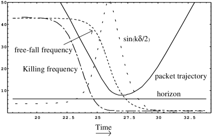
FIG. 4.: WKB evolution.

Notice first the behavior of $\sin(k\delta/2)$. Backwards in time this starts out very small, rises to the maximum, and comes back down but not to zero. The group velocity in the frame falling with the lattice vanishes at the top, when $k\delta/2=\pi/2$, corresponding to a wavelength equal to two lattice units. This rise and fall happens via a monotonic change of $k$, and is the Bloch oscillation mentioned above.

The wavepacket that ends up with $\omega=\omega_{K}=1$ at late times starts out at early times with $\omega=\omega_{K}\sim 43$. The maximum possible lattice frequency is $2/\delta=500$ in this case, so the ingoing frequency is certainly “high”. Whereas the free-fall frequency continues to redshift (forward in time) as the wavepacket climbs away from the horizon, the redshifting of the Killing frequency is essentially complete by the time the wavepacket reaches the turning point. Thus, past the turning point, each Killing frequency component propagates autonomously, more or less as it would in the continuum. As described in the Introduction, this, together with the fact that the evolution of $\omega$ at the lattice scale is adiabatic, is the reason why the usual Hawking effect is reproduced.

IV LATTICE WAVE EQUATION ANALYSIS

In this section we discuss the results of our numerical calculations. The basic method is to take an outgoing positive frequency wavepacket and evolve it backwards in time. After it has “bounced” from the horizon and propagated back into the flat region of the spacetime we decompose it into positive and negative frequency parts. Since it is a purely left moving wavepacket at this stage the negative frequency part is just the part composed of positive wavevectors. The occupation number (21) of the original outgoing packet is then given by minus the norm of this negative frequency part divided by the total norm. We typically computed the total norm in position space using (18). Since the negative frequency part $\varphi^{(-)}$ was projected out in the wavevector space we used an alternate expression for its norm, $(\varphi^{(-)},\varphi^{(-)})=-2\sum_{k>0}|\omega(k)||\widetilde{\varphi}^{(-)}(k)|^{2}$, where the frequency $\omega(k)$ is given by (23).

A Numerical issues

Our system of equations (17) is a coupled set of ordinary differential equations, which is to be solved in the limit that time is continuous but the spatial lattice is fixed. In order to satisfy the Courant stability criterion the time step $\Delta t$ must satisfy $\Delta t<a(z,t)\delta$. (In this 1+1 dimensional setting the Courant condition coincides with the condition that causality be respected by the differencing scheme.) In the asymptotic region $a(z,t)=1$ so the stability condition there is $\Delta t<\delta$. For a fixed $\Delta t/\delta$ the general condition would be violated wherever $a(z,t)<\Delta t/\delta$. Since this only happens deep behind the horizon (for $t>0$) we just modified $a(z,t)$ inside the black hole so that it is never less than $\Delta t/\delta$. We used a time discretization scheme (written out in the Appendix) with errors of order $(\Delta t)^{2}$, and found that $\Delta t=0.4\delta$ was adequately small to obtain very good accuracy.

B Wavepackets and parameters

If the Killing frequency were conserved as it is in the dispersive continuum models the entire Hawking spectrum could be probed just by propagating one wavepacket and decomposing it into is Fourier components, each of which would pick up a negative frequency part appropriate for the corresponding frequency. This is how Unruh checked the spectrum in his model[6]. Since the Killing frequency is not conserved on our lattice we cannot avail ourselves of this option. Thus instead we compute the occupation numbers for a sequence of wavepackets $\widetilde{\varphi}_{s}(k)$ with different profiles:

$$\widetilde{\varphi}_{s}(k)=k\,\exp[-(k-0.05s)^{2}],\qquad s=1,\dots,9$$ (26)

(in units with $\kappa=1$, as usual). The form of these wavepackets was dictated by the need to have them well enough localized to be contained in the flat region of the spacetime (so we could construct the corresponding positive frequency initial data) while at the same time containing enough power at low frequencies of order $\kappa$ to have a measurable Hawking occupation number. To shift the wavepacket to the desired starting position the Fourier transform (26) was multiplied by a phase factor $\exp(-ikz_{\rm initial})$. The positive frequency initial data was constructed by evolving each Fourier component one time step $\Delta t$ by multiplying with the phase factor $\exp(-i\omega(k)\Delta t)$ and Fourier transforming the result back into position space.

The time dependence of the lattice (illustrated in Fig. 1) means that the results will not be independent of the “launch time” of the wavepacket from a given location. If we start our backwards evolution too far in the future then when the wavepacket nears the horizon the lattice points will be pathologically sparse. On the other hand if we launch backwards at too early a time then the wavepacket can become partially trapped in the region where the lattice spacing gets very small. This happens because a sufficiently high frequency wave is turned around when it tries to propagate into a region of larger lattice spacing. We encountered this “channeling” phenomenon in our simulations, and avoided it just by launching later. The runs reported here were all done with wavepackets that reached the horizon around $t=27$, and were launched from far enough away to be contained in the flat region of the spacetime. Typically, the launch time was around $t=56$ when the wavepacket was centered at $x=28$.

All of the calculations reported here were done using the line element (1), with $v_{\rm max}$ (4) ranging from $\sqrt{2}$ to $30$.

C Results

1 Generalities

The behavior of a typical wavepacket throughout the process of bouncing off the horizon is illustrated in Fig. 6. The real part of the wavepacket is plotted vs. the static coordinate $x$ at several different times. Following backwards in time, the wave starts to squeeze up against the horizon and then a trailing dip freezes and develops oscillations that grow until they balloon out, forming into a compact high frequency wavepacket that propagates neatly away from the horizon backwards in time.

This ingoing wavepacket contains both positive and negative frequency components, in just the right combination to produce only an outgoing wave when sent in towards the black hole, with no wave propagating across the horizon. To illustrate this we have taken one of these ingoing wavepackets, decomposed it into its positive and negative frequency parts, and sent them separately back toward the horizon forward in time (Fig. 7). The negative frequency part (which is the smaller of the two since the surface gravity is fairly low compared to the typical frequencies in the outgoing wavepacket), mostly crosses the horizon, with just a bit bouncing back out. The positive frequency part mostly bounces, with just a little bit going into the black hole.

2 Spectrum

The “observed” occupation numbers for the wavepackets (26) all agree well with the integrated thermal predictions (22) of the Hawking effect provided the lattice spacing is not too large.

TABLE I.: Comparison of the black hole radiation on the lattice to the thermal Hawking occupation numbers (22) for the wavepackets (26) for the case $v_{\rm max}=\sqrt{2}$ and $\kappa\delta=0.002$.

s	Thermal	Lattice	Rel. Diff.
1	0.01563	0.01557	0.0038
2	0.01409	0.01404	0.0035
3	0.01266	0.01262	0.0034
4	0.01135	0.01130	0.0041
5	0.01014	0.01009	0.0045
6	0.00903	0.00899	0.0039
7	0.00801	0.00797	0.0051
8	0.00709	0.00705	0.0052
9	0.00625	0.00622	0.0046

A sample of the comparisons for $\kappa\delta=0.002$ is listed in Table I. The typical relative difference in this case is of order half a percent.

3 Lattice dependence

To study the dependence on the lattice we ran the $s=1$ wavepacket backward at several different values of the lattice spacing and for several values of $v_{\rm max}$ (4) from $\sqrt{2}$ to 30. The change of $v_{\rm max}$ produces only a rather small change in the shape of the function $v(x)$ outside the horizon, however it produces a shift of the position of the horizon (5). For large $v_{\rm max}$ the horizon is given approximately by $x_{H}\simeq\ln(2v_{\rm max})$. The horizon position ranges from about 0.6 for $v_{\rm max}=\sqrt{2}$ to about 4 for $v_{\rm max}=30$. Thus a wavepacket launched backward in time from a given position at a given time will reach the horizon later in time for larger $v_{\rm max}$, so that the proper lattice spacing at the horizon will be larger, though not by a very large amount for the wavepackets considered here.

In Fig. 5 we plot the occupation numbers for lattice spacings $\delta$ ranging from 0.002 to 0.128, and for several values of $v_{\rm max}$ (4), $v_{\rm max}=\sqrt{2},2,2.5,3,4,5,10,20,30$. In all cases the late time wavepacket was launched from the same position and time. All wavepackets had the same envelope for their Fourier transform, however for different lattice spacings the wavepacket is necessarily different.

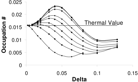
FIG. 5.: Occupation numbers for $s=1$ wavepacket for various values of $\delta$ and $v_{\rm max}$. Higher occupation numbers correspond to larger values of $v_{\rm max}$.

For all values of $v_{\rm max}$, the occupation number converges to the Hawking prediction as the lattice spacing $\delta$ decreases.

The pattern of deviations from the thermal prediction appears to depend quite strongly on the value of $v_{\rm max}$, a result which we do not understand at present. The best we can do is to list various effects which would contribute to the deviations: (i) the WKB turning point is moving away from the horizon as $\delta$ grows, so one might expect that the effective surface gravity $v^{\prime}(x_{\rm t.p.})$ and hence the effective Hawking temperature felt by the wavepacket would decrease; (ii) at larger $v_{\rm max}$ the proper lattice spacing at the horizon is larger at the time this particular wavepacket reaches the horizon; (iii) the lattice points are rather sparse near the horizon for the larger values of $\delta$, and their precise positions will be significantly different for different values of $v_{\rm max}$. Effect (i) would lead to a decrease in the occupation number, while one might expect that effect (ii) would lead to a relative increase due to the extra particle creation associated with time dependence of the lattice. Perhaps what we are seeing is just a delicate balance between these two effects.

V DISCUSSION

We have shown that linear field theory on a falling lattice reproduces the continuum Hawking effect with high fidelity, thus verifying earlier expections[12]. For the smallest lattice spacing we studied, $\delta=0.002/\kappa$, the deviations from the thermal particle creation in wavepackets composed of frequencies $\omega\;\raisebox{-3.44444pt}{$\stackrel{{\scriptstyle\textstyle<}}{{\sim}}$}\;O(\kappa)$ were of order half a percent. This is remarkable, particularly since the proper lattice spacing encountered by the wavepacket at the horizon was $\sim 0.08/\kappa$. When $\kappa\delta$ is pushed to higher values eventually we see significant deviations from the Hawking prediction.

There are several directions in which this work could be developed. One idea is to include self-interactions for the quantum field theory. There are general arguments[21, 22] that the thermal Hawking effect holds also for interacting fields. There are also perturbative calculations[23] and calculations exploiting exact conformal invariance of certain 1+1 dimensional field theories[24]. Also the “hadronization” of Hawking radiation from primordial black holes has been analyzed by matching to high energy collision data[25], but the physics of how the thermal Hawking radiation is “dressed” by interactions as it redshifts away from the horizon has not been studied. In a 1+1 dimensional model it should not be prohibitively difficult to numerically study Hawking radiation of interacting fields, now that we see it can be done on a lattice.

The falling lattice model has provided a satisfactory mechanism—the Bloch oscillation—for how to get an outgoing mode from an ingoing mode in a stationary background, but there is a serious flaw in the picture: the lattice is constantly expanding. In the fluid model by contrast the lattice of atoms maintains a uniform average density. In a fundamental theory we might also expect the scale of graininess of spacetime to remain fixed at, say, the Planck scale or the string scale (since presumably the graininess would define this scale) rather than expand. Can the falling lattice model be improved to share this feature?

A fluid maintains uniform density in an inhomogeneous flow by compressing in some directions and expanding in others, which requires at least two dimensions to be possible. At the atomic level such a volume-preserving flow involves erratic motions of individual atoms. One possible improvement of the lattice model is to make a lattice that mimics this sort of volume preserving flow. It is not clear whether the motions of the lattice points can be slow enough to be adiabatic on the timescale of the high frequency lattice modes. If they cannot, then the time dependence of this erratic lattice background will excite the quantum vacuum.

In a fluid the lattice is a part of the system, not just a fixed background. The average flow could be adiabatic for the fully coupled ground state of the system but not for the field theory of the perturbations on the “background lattice”. Similar comments apply in quantum gravity: surely if in-out mode conversion is at play the incoming high frequency modes are strongly coupled to the quantum gravitational vacuum. Ideally, therefore, we should try to find a model in which the background is not decoupled from the perturbations.

As a first step in this direction one could study a one dimensional model in which the lattice points are non-relativistic point masses, coupled to each other by nearest neighbor interactions, and “falling” or propagating in a background potential (with or without periodic boundary conditions). The perturbations of such a lattice are the phonon field, and the back reaction to the Hawking radiation is included (although the background potential is fixed). In a model like this one could presumably follow in detail the nonlinear origin of the outgoing modes and the transfer of energy from the mean flow to the thermal radiation.

Finite differencing scheme

The equation of motion (17) for $\varphi_{m}(t)$ is

$$\partial_{t}\Bigl{(}a_{m}(t)\partial_{t}\varphi_{m}(t)\Bigr{)}=D\left(\frac{2D\varphi_{m-1}(t)}{a_{m+1}(t)+a_{m}(t)}\right).$$ (27)

We used a time discretization scheme for the left hand side arising from the replacement of $\dot{f}$ by

$$\Bigl{[}f(t+\Delta t/2)-f(t-\Delta t/2)\Bigr{]}/\Delta t=\dot{f}+(1/24){f}^{(3)}(\Delta t)^{2}+O((\Delta t)^{4}),$$ (28)

which yields

$$\partial_{t}(a_{m}(t)\partial_{t}\varphi_{m}(t))\rightarrow\Bigl{[}a(n+1/2)\Bigl{(}\varphi(n+1)-\varphi(n)\Bigr{)}-a(n-1/2)\Bigl{(}\varphi(n)-\varphi(n-1)\Bigr{)}\Bigr{]}/(\Delta t)^{2},$$ (29)

where the spatial index is omitted and the argument $n$ stands for $n\Delta t$. We could have used this replacement, since $a(z,t)$ is a prescribed function that can be calculated at any $t$, but for some reason we substituted $a(n\pm 1/2)$ by the average $\Bigl{(}a(n)+a(n\pm 1)\Bigr{)}/2$. This yields the approximation

$$\Bigl{[}\Bigl{(}a(n)+a(n+1)\Bigr{)}\Bigl{(}\varphi(n+1)-\varphi(n)\Bigr{)}-\Bigl{(}a(n)+a(n-1)\Bigr{)}\Bigl{(}\varphi(n)-\varphi(n-1)\Bigr{)}\Bigr{]}/2(\Delta t)^{2}$$ (30)

$$=\partial_{t}(a\partial_{t}\varphi)(n)+\Bigl{(}\frac{1}{12}{a}{\varphi}^{(4)}+\frac{1}{6}\dot{a}{\varphi}^{(3)}+\frac{1}{4}\ddot{a}\ddot{\varphi}+\frac{1}{4}{a}^{(3)}\dot{\varphi}\Bigr{)}(n)(\Delta t)^{2}+O((\Delta t)^{4}).$$ (31)

With (30) in place of the left hand side of (27) we solve for $\varphi(n-1)$ in terms of $\varphi(n)$ and $\varphi(n+1)$ to obtain an equation for evolving $\varphi$ backwards in time by one time step given the following two steps.

FIG. 6.: A typical wavepacket evolution. Here $v_{\rm max}=\sqrt{2}$, $\kappa\delta=0.004$, and the wavepacket (26) has $s=1$. The ocsillations of the incoming wavepacket are too dense to resolve in the plots.

FIG. 7.: The positive (top row) and negative (bottom row) frequency parts of the ancestor of an outgoing positive frequency wavepacket, sent back towards the black hole. Note the vertical scale is different in the two plots. The wavepackets crossing the horizon in the two cases are negatives of each other since they must cancel to produce only the outgoing wavepacket we started with. The parts that go through the horizon appear on the right due to periodic boundary conditions. The high frequency ocsillations are too dense to resolve in the plots.

REFERENCES

- [1] T. Jacobson, Phys. Rev. D44, 1731 (1991).
- [2] For a review see A.W. Peet, Class. Quant. Grav. 15, 3291 (1998).
- [3] W.G. Unruh, Phys. Rev. Lett. 46, 1351 (1981).
- [4] V. Moncrief, Astrophys. J, 235, 1038 (1980).
- [5] M. Visser, Class. Quantum Grav. 15, 1767 (1998).
- [6] W.G. Unruh, Phys. Rev. D 51, 2827 (1995).
- [7] R. Brout, S. Massar, R. Parentani and Ph. Spindel, Phys. Rev. D 52, 4559 (1995).
- [8] S. Corley and T. Jacobson, Phys. Rev. D 54,1568 (1996).
- [9] S. Corley, Phys. Rev. D 57, 6280 (1998).
- [10] Y. Himemoto and T. Tanaka, “A generalization of the model of Hawking radiation with modified high frequency dispersion relation”, gr-qc/9904076.
- [11] H. Saida and M. Sakagami, “Black hole radiation with high frequency dispersion”, gr-qc/9905034.
- [12] S. Corley and T. Jacobson, Phys. Rev. D 57, 6269 (1998).
- [13] T.A. Jacobson and G.E. Volovik, Phys. Rev. D 58, 064021 (1998); JETP Lett. 68, 874 (1998).
- [14] N.B. Kopnin and G.E. Volovik, Phys. Rev. B 57, 8526 (1998); Phys. Rev. Lett. 79, 1377 (1997).
- [15] G.E. Volovik, Pis’ma Zh. Eksp. Teor. Fiz. 69, 662 (1999) [JETP Lett. 69, 705 (1999).]
- [16] S. Corley, Phys. Rev. D 57, 6280 (1998).
- [17] T. Jacobson, Phys. Rev. D 53 (1996) 7082.
- [18] See e.g. Appendix A of ref. [12].
- [19] S.W. Hawking, Nature (London) 248 (1974) 30; Commun. Math. Phys. 43 (1975) 199.
- [20] The Hamiltonian technique was first applied to dispersive models of the Hawking effect in ref. [7].
- [21] G.W. Gibbons and M.J. Perry, Proc. Roy. Soc. Lond., Series A 358, 467-94 (1977).
- [22] W.G. Unruh and N. Weiss, Phys. Rev. D 29, 1656 (1984).
- [23] D.A. Leahy and W.G. Unruh, Phys. Rev. D 28, 694 (1983).
- [24] N.D. Birrell and P.C.W. Davies, Phys. Rev. D 18, 4408 (1978).
- [25] J.H. MacGibbon and B.R. Webber, Phys. Rev. D 41, 3052 (1990); J.H. MacGibbon, Phys. Rev. D 44, 376 (1991); F. Halzen, E. Zas, J.H. MacGibbon, and T.C. Weekes, Nature 353, 807 (1991).