August 1999 TAUP–2582–99

We show that supersymmetry Ward identities contain an anomalous term which takes the form of a surface term in Hilbert space. In the one-instanton sector the anomalous term is the integral of a total $\rho$-derivative where $\rho$ is the instanton’s size. There are cases where the anomalous term is non-zero, and cannot be modified by subtractions. This constitutes a supersymmetry anomaly. The derivation is based on Feynman rules suitable for any non-perturbative sector of a weakly-coupled, renormalizable gauge theory.

1.  Introduction

Following ’t Hooft’s pioneering work [1], instanton physics has played an important role in understanding the dynamics of asymptotically-free theories. Mostly, explicit instanton calculations were limited to the semi-classical approximation. A two-loop calculation which is particularly relevant for supersymmetry (SUSY) can be found in ref. [2].

There is no consistent regularization method which preserve SUSY [3]. In this sense, SUSY is similar to a chiral symmetry. Whether SUSY is a true symmetry at the quantum level, or not, can be decided only by non-perturbative studies. This question was previously addressed in the semi-classical approximation, where it was found that SUSY is preserved. Important works are based on the assumption that this remains true beyond the semi-classical approximation, and that SUSY is an exact symmetry in the continuum limit [4-10].

We begin with the investigation of Ward identities in the most general path integral setting. A Ward identity reads

$$\left\langle\mbox{\boldmath$\delta$}{\cal O}\right\rangle=\left\langle\mbox{\boldmath$\delta$}S\;{\cal O}\right\rangle+\left\langle\mbox{\boldmath$\delta$}\mu\;{\cal O}\right\rangle+\left\langle\,\mbox{\rm Hilbert-space surface terms}\,\right\rangle\,,$$ (1.1)

where the bold letter $\delta$ denotes any infinitesimal transformation. Besides the familiar terms containing the variations of the action ($\mbox{\boldmath$\delta$}S$) and the measure ($\mbox{\boldmath$\delta$}\mu$), eq. (1.1) contains also (the expectation value of) Hilbert-space surface terms, which arise from integration by parts in the functional integral.

In more detail, in each non-perturbative sector the path integration is over a given set of collective coordinates $\zeta_{n}$ that characterize the classical background, as well as over the amplitudes of the quantum-field modes. The expectation value of a (gauge invariant) operator ${\cal O}$ is

$$\left\langle{\cal O}\right\rangle=\int d^{n}\zeta\;e^{-S_{\rm cl}-W_{1}-W_{2}}\,\left\langle{\cal O}\right\rangle_{\!\zeta}\,.$$ (1.2)

Here $S_{\rm cl}$ is the classical action, and the semi-classical measure, $\exp(-W_{1})$, is the product of functional determinants and a tree-level jacobian [1]. $W_{2}$ is the sum of all connected bubble diagrams, and $\left\langle{\cal O}\right\rangle_{\!\zeta}$ is the sum of all diagrams with external legs defined by the operator ${\cal O}$. All diagrams are obtained here by integrating over the quantum fields, keeping the collective coordinates fixed. Eq. (1.2) applies to both bare and renormalized quantities.

Eq. (1.1) is derived in Sec. 2. Restricting our attention to the SUSY variation, which we denote $\delta$, we write $\delta S$ and $\delta\mu$ as spectral sums, and show that they both vanish mode by mode. Thus, $\big{\langle}\delta{\cal O}\big{\rangle}$ may fail to be zero only due to the Hilbert-space surface term. Explicitly

$$\left\langle\delta{\cal O}\right\rangle=\int d^{n}\zeta\;{\partial\over\partial\zeta_{n}}\left(e^{-S_{\rm cl}-W_{1}-W_{2}}\,\left\langle\delta\zeta_{n}\,{\cal O}\right\rangle_{\!\zeta}\right)\,,$$ (1.3)

where $\delta\zeta_{n}$ is the SUSY variation of the $n$-th collective coordinate.

The tools of functional differentiation and integration used in Sec. 2 are very useful in clarifying the algebraic structure that underlies eq. (1.3). However, manipulations of the (formal) path integral should be supported by a detailed diagrammatic calculation. In Sec. 3 we turn to the instanton sector of four-dimensional SUSY gauge theories. Only the integral of the total $\rho$-derivative is not automatically zero ($\rho$ is the instanton size). The anomalous term may thus be represented as an amplitude involving a zero-size instanton. An anomaly due to a topological singularity was previously found in supersymmetric quantum mechanics in the presence of fluxons with a fractional magnetic flux [11].

We consider the SUSY Ward identity (1.3) at the leading non-trivial order for a specific bi-local operator in super Yang-Mills theory. Our main result is the anomalous Ward identity eq. (3.10), and its local version eq. (3.38). Both equations are valid in any renormalization prescription where perturbation theory is supersymmetric. While the leading contribution to the $\rho\to 0$ surface term on the r.h.s. of eq. (3.10) is a tree diagram, a straightforward calculation of the expectation value of $\delta{\cal O}$ involves loop diagrams. The proof of eq. (3.10) thus requires careful separation of short- and long-distance contributions. We also generalize the result to supersymmetric QCD. An important question is how eq. (3.10) is modified by higher-order corrections. A renormalization-group argument indicates that the anomalous term should remain finite (and non-zero) after the inclusion of next-order logarithmic corrections.

The limit of a vanishing instanton size, $\rho\to 0$, is studied in more detail in Sec. 4. In correlation functions involving operators of sufficiently high dimension, the lower limit of the $\rho$-integral may diverge. Under these circumstances one should perform non-perturbative subtractions. Our main result is that no non-perturbative subtraction can possibly modify eq. (3.10). Therefore eq. (3.10) constitutes a supersymmetry anomaly. We also discuss how the anomaly should arise on the lattice.

There are important non-perturbative sectors where one is not expanding around an exact solution of the classical field equations. This is true in the one-instanton sector of theories with a scalar (Higgs) VEV, as well as in the instanton-antiinstanton sector. Aiming to cover these cases too, we have developed Landau-gauge Feynman rules for any non-perturbative sector of a renormalizable gauge theory (Appendix B). The Feynman rules define a systematic expansion provided the considered correlation function is infra-red convergent, and provided the background field is “almost” a classical solution.

Affirming the validity of the perturbative expansion must be done on a case by case basis. (A more detailed discussion of the one-instanton sector of SUSY-Higgs theories will be given elsewhere.) However, the basic Ward identity (1.3) can be derived in a completely general way using the Feynman rules of Appendix B. This is done in Appendix C. We give a fully detailed diagrammatic derivation in the (physically less interesting) case of a theory without a gauge symmetry. Because of its technical complexity, we outline the generalization to gauge theories but omit the arithmetical details.

Much of the technical material contained in this paper is devoted to various detailed proofs. A first acquaintance with the algebraic structure may be obtained by reading Sec. 2 up to subsection 2.2. In order to understand the content of eq. (3.10) it is enough to read Sec. 3 up to subsection 3.1. The local form of eq. (3.10) is discussed in subsection 3.5, and the renormalization-group argument is given in subsection 3.6. The proof that eq. (3.10) cannot be modified by subtractions is given in subsection 4.1.

The notation used throughout the paper is defined in Appendix A. In Appendix D we explain how the general formalism of Sec. 2 works in the case of translation invariance. Our conclusions are given in Sec. 5.

2.  Path-integral derivation of SUSY Ward identities

In this section we derive the anomalous Ward identity (1.3) using the tools of functional integration and differentiation. While the (unregularized) path integral is a formal construct, the derivation serves to clarify both the underlying algebraic structure, and the role of physical boundary conditions. The results of this section are supported by the detailed diagrammatic calculations of Sec. 3 and Appendix C.

The notation of Appendix A is used below. The general and the SUSY Ward identities (eqs. (1.1) and (1.3) respectively) will be derived using the transverse-field path integral defined in the first four subsections of Appendix B. (The rest of Appendix B, which is devoted to the construction of the tree-level propagators etc., is not needed for this section.)

2.1. The field variation

The independent variables of the path integral include the collective coordinates $\zeta_{n}$, the gauge degrees of freedom $\omega^{a}(x)$, and the amplitudes of the quantum modes $\hat{\beta}_{p}$ and $\hat{\Psi}_{p}$ where

$$\hat{\beta}(x)\equiv\sum_{p}\int\hskip 4.2679pt\chi^{B}_{p}(x)\hat{\beta}_{p}\,,\qquad\hat{\Psi}(x)\equiv\sum_{p}\int\hskip 4.2679pt\chi^{F}_{p}(x)\hat{\Psi}_{p}\,,$$ (2.1)

and $\chi^{B}_{p}(x)$ ($\chi^{F}_{p}(x))$ is the eigenfunction corresponding to $\hat{\beta}_{p}$ ($\hat{\Psi}_{p}$). In this paper the quantum bosonic field, $\hat{\beta}(x)$, is assumed to be transverse. Namely, it obeys the background gauge condition $\Omega^{\dagger a}\hat{\beta}(x)=0$ (eq. (B.5)) in addition to the orthogonality conditions $\mbox{\large\boldmath$($}b_{;m}\mbox{\large\boldmath$|$}\hat{\beta}\mbox{\large\boldmath$)$}=0$ (eq. (B.16)) where $b_{;m}$ is the covariant derivative of the classical field with respect to $\zeta_{m}$. The above constraints may be summarized as $\mbox{\large\boldmath$($}b_{;{\scriptscriptstyle M}}\mbox{\large\boldmath$|$}\hat{\beta}\mbox{\large\boldmath$)$}=0$, where the capital index ${\scriptstyle M}$ runs over the ordinary collective coordinates and over the infinitely-many collective coordinates associated with local gauge transformations, see Appendix B.4.

We begin by expanding an arbitrary variation of an elementary field in terms of variations of the independent path-integral variables. For the variation of a boson field, $\mbox{\boldmath$\delta$}B(x)$, one has

$$\mbox{\boldmath$\delta$}B(x)=\mbox{\boldmath$\delta$}\hat{\beta}(x)+\left(b_{;n}(x)+\hat{\beta}_{;n}(x)\right)\mbox{\boldmath$\delta$}\zeta_{n}+\left(\Omega^{a}(b(x))-igT^{a}\hat{\beta}(x)\right)\mbox{\boldmath$\delta$}\omega^{a}(x)\,.$$ (2.2)

Covariant $\zeta_{n}$-derivatives of the quantum field are obtained by differentiating the eigenfunctions (see also Appendix B.3)

$$\hat{\beta}_{;n}(x)=\sum_{p}\int\hskip 4.2679pt\chi^{B}_{p;n}(x)\,\hat{\beta}_{p}\,,$$ (2.3)

while the quantum-field variation is, by definition

$$\mbox{\boldmath$\delta$}\hat{\beta}(x)\equiv\sum_{p}\int\hskip 4.2679pt\chi^{B}_{p}(x)\,\mbox{\boldmath$\delta$}\hat{\beta}_{p}\,.$$ (2.4)

The field variation acts on the quantum amplitudes $\hat{\beta}_{p}$ and not on the eigenfunctions. The differential operator $\Omega^{a}$ generates infinitesimal gauge transformations of the classical bosonic field (Appendix B.1). The variation of a fermion field, $\mbox{\boldmath$\delta$}\Psi(x)$, is expanded as

$$\mbox{\boldmath$\delta$}\Psi(x)=\mbox{\boldmath$\delta$}\hat{\Psi}(x)+\mbox{\boldmath$\delta$}\zeta_{n}\,\hat{\Psi}_{;n}(x)-ig\,\mbox{\boldmath$\delta$}\omega^{a}(x)\,T^{a}\,\hat{\Psi}(x)\,,$$ (2.5)

where

$$\hat{\Psi}_{;n}(x)=\sum_{p}\int\hskip 4.2679pt\chi^{F}_{p;n}(x)\,\hat{\Psi}_{p}\,,\qquad\mbox{\boldmath$\delta$}\hat{\Psi}(x)\equiv\sum_{p}\int\hskip 4.2679pt\chi^{F}_{p}(x)\,\mbox{\boldmath$\delta$}\hat{\Psi}_{p}\,,$$ (2.6)

in analogy with the bosonic case. (The reader should note that $\mbox{\boldmath$\delta$}\Psi(x)$ and $\mbox{\boldmath$\delta$}\hat{\Psi}(x)$ have different meanings.) For the SUSY variation, ordering matters in eq. (2.5). It follows from eq. (2.4) that $\mbox{\boldmath$\delta$}\hat{\beta}(x)$ obeys the same orthogonality constraints as does $\hat{\beta}(x)$. This allows us to extract the variations $\mbox{\boldmath$\delta$}\zeta_{n}$ and $\mbox{\boldmath$\delta$}\omega^{a}(x)$. Considering eq. (2.2) and taking the inner product (A.5) with $b_{;n}$ leads to

$$\delta\zeta_{m}=C^{-1}_{mn}\left\{\raisebox{0.0pt}{\Large\boldmath$($}b_{;n}\raisebox{0.0pt}{\Large\boldmath$|$}\Gamma\hat{\Psi}\raisebox{0.0pt}{\Large\boldmath$)$}+ig\raisebox{0.0pt}{\Large\boldmath$($}b_{;n}^{\dagger}T^{a}\hat{\beta}\raisebox{0.0pt}{\Large\boldmath$|$}\delta\omega^{a}\raisebox{0.0pt}{\Large\boldmath$)$}\right\}\,,$$ (2.7)

where $C_{mn}$ is defined in eq. (B.14) and we have used eq. (B.7). We have specialized to the SUSY case, where the bosons’ variation is linear in the fermions, see eq. (A.7). (For any other variation, simply replace $\delta\to\mbox{\boldmath$\delta$}$ and $\Gamma\hat{\Psi}\to\mbox{\boldmath$\delta$}B$.) Note that $b_{;n}$ is $O(1/g)$, and $\delta\zeta_{m}$ is $O(g)$. We next apply $\Omega^{\dagger}$ on both sides of eq. (2.2). Using the gauge-fixing constraint (B.5) and eliminating $\delta\zeta_{m}$ we find

$$\delta\omega^{a} = ({\cal F}^{-1})^{ab}\raisebox{0.0pt}{\Large\boldmath$|$}\Omega^{b\dagger}\,\Gamma\hat{\Psi}\raisebox{0.0pt}{\Large\boldmath$)$}$$ (2.8)

$$+ig({\cal F}^{-1})^{ab}\raisebox{0.0pt}{\Large\boldmath$|$}b_{;m}^{\dagger}T^{b}\hat{\beta}\raisebox{0.0pt}{\Large\boldmath$)$}\,C^{-1}_{mn}\,\raisebox{0.0pt}{\Large\boldmath$($}b_{;n}\raisebox{0.0pt}{\Large\boldmath$|$}\Gamma\hat{\Psi}\raisebox{0.0pt}{\Large\boldmath$)$}\,.$$

Here ${\cal F}^{-1}={\cal F}_{0}^{-1}-{\cal F}_{0}^{-1}{\cal F}_{\rm int}{\cal F}_{0}^{-1}+\cdots$, where ${\cal F}_{0}$ and ${\cal F}_{\rm int}$ occur respectively in the tree-level and interaction ghost lagrangians (eq. (B.36)). Eqs. (2.7) and (2.8) are summarized by the compact formula (cf. eq. (B.31))

$$\delta\zeta_{\scriptscriptstyle M}={\cal C}^{-1}_{\scriptscriptstyle MN}\raisebox{0.0pt}{\Large\boldmath$($}b_{;{\scriptscriptstyle N}}\raisebox{0.0pt}{\Large\boldmath$|$}\Gamma\hat{\Psi}\raisebox{0.0pt}{\Large\boldmath$)$}\,.$$ (2.9)

The variation of a given quantum amplitude is obtained by taking the inner product of eq. (2.2) or (2.5) with the corresponding eigenmode. Explicitly,

$$\delta\hat{\beta}_{p}=\raisebox{0.0pt}{\Large\boldmath$($}\chi^{B}_{p}\raisebox{0.0pt}{\Large\boldmath$|$}\Gamma\hat{\Psi}\raisebox{0.0pt}{\Large\boldmath$)$}-\delta\zeta_{\scriptscriptstyle M}\raisebox{0.0pt}{\Large\boldmath$($}\chi^{B}_{p}\raisebox{0.0pt}{\Large\boldmath$|$}\hat{\beta}_{;{\scriptscriptstyle M}}\raisebox{0.0pt}{\Large\boldmath$)$}\,,$$ (2.10)

for bosons, and

$$\delta\hat{\Psi}_{p}=\raisebox{0.0pt}{\Large\boldmath$($}\chi^{F}_{p}\raisebox{0.0pt}{\Large\boldmath$|$}\delta\Psi\raisebox{0.0pt}{\Large\boldmath$)$}-\delta\zeta_{\scriptscriptstyle M}\raisebox{0.0pt}{\Large\boldmath$($}\chi^{F}_{p}\raisebox{0.0pt}{\Large\boldmath$|$}\hat{\Psi}_{;{\scriptscriptstyle M}}\raisebox{0.0pt}{\Large\boldmath$)$}\,.$$ (2.11)

For fermions. The last term is these equations compensates for the $\zeta_{\scriptscriptstyle M}$-dependence of the eigenmodes.

2.2. Ward identities

The variation of any local operator can be expressed in terms of the variations of the independent variables. One has

$$\delta{\cal O}={\cal T}{\cal O}\,,$$ (2.12)

where ${\cal T}$ is the functional differentiation operator

$${\cal T}=\sum_{p}\int\hskip 4.2679pt\delta\hat{q}_{p}{\partial\over\partial\hat{q}_{p}}+\sum_{\scriptscriptstyle N}\int\hskip 4.2679pt\delta\zeta_{\scriptscriptstyle N}\,{\partial\over\partial\zeta_{\scriptscriptstyle N}}\,,$$ (2.13)

and $\hat{q}_{p}$ stands for any quantum-field amplitude, cf. Appendix B.3. In practice we will be interested in gauge invariant operators, which effectively restricts the last sum to ${\scriptstyle N}=n$ only. The expectation value of $\delta{\cal O}$ is given by the functional integral (eq. (B.33))

$$\left\langle\delta{\cal O}\right\rangle=\int d^{n}\zeta\;{\cal D}\hat{q}\,\,{{\rm Det}\,{\cal C}\over{\rm Det}^{1\over 2}\,{\cal C}_{0}}\,\,e^{-S}\,\,{\cal T}{\cal O}\,.$$ (2.14)

Integrating by parts we obtain the generic Ward identity for gauge invariant operators

$$\left\langle\delta{\cal O}\right\rangle=\left\langle\delta S\;{\cal O}\right\rangle+\left\langle\delta\mu\;{\cal O}\right\rangle+\int d^{n}\zeta\;{\partial\over\partial\zeta_{n}}\left\{\int{\cal D}\hat{q}\,\,{{\rm Det}\,{\cal C}\over{\rm Det}^{1\over 2}\,{\cal C}_{0}}\;e^{-S}\;\delta\zeta_{n}\,{\cal O}\right\}\,,$$ (2.15)

where $\delta S$ and $\delta\mu$ are respectively the variations of the action and the measure. Explicitly $\delta S={\cal T}S$ and

$$-\delta\mu\equiv{\cal T}\log\left\{{{\rm Det}\,{\cal C}\over{\rm Det}^{1\over 2}\,{\cal C}_{0}}\right\}+\sum_{p}\int\hskip 4.2679pt{\partial(\delta\hat{q}_{p})\over\partial\hat{q}_{p}}+{\partial(\delta\zeta_{n})\over\partial\zeta_{n}}\,.$$ (2.16)

The last term on the r.h.s. of eq. (2.15) is the Hilbert-space surface term of eq. (1.1). The corresponding surface term for the quantum amplitudes $\hat{q}_{p}$ is zero because of the Gaussian integration.

In the rest of this section we consider SUSY Ward identities. We compute $\delta S$ and $\delta\mu$, and prove that they both vanish mode by mode. This leaves us with the last term in eq. (2.15). When the functional integration over the quantum fields is done, this term is recognized as the r.h.s. of eq. (1.3).

The SUSY transformation is off-diagonal in that it maps bosons into fermions and vice versa. In view of this, the invariance of the measure, $\delta\mu=0$, is an expected result. Nevertheless, the below derivation gives us valuable information on how the cancelation of the various contributions to $\delta\mu$ works in practice. We also find that the physical boundary conditions play a direct role. The same elements reappear in the diagrammatic proof of Appendix C which is more rigorous and, at the same time, technically more involved.

The presence of a Hilbert-space surface term in Ward identities is not an unfamiliar situation. In appendix D we apply the generic Ward identity (2.15) to the case of translation invariance. We show that momentum is conversed because the Hilbert-space surface term coincides in this case with a spacetime surface term.

2.3. Variation of the action

The functional variation of the action consists of a volume integral and a surface integral. The latter may in general depend on the choice of functional variables, and it is our objective to determine it. We start with the action principle

$$\int d^{d}x\,\left(\delta{\cal L}-\partial_{\mu}(\delta Q\,\Pi_{\mu})\right)=\int d^{d}x\,\delta Q\left(-\Pi_{\mu;\mu}+\partial{\cal L}/\partial Q\right)\,.$$ (2.17)

As usual ${\cal L}={\cal L}(Q,Q_{,\mu})$ and $\Pi_{\mu}=\partial{\cal L}/\partial{Q_{,\mu}}$. Substituting eqs. (2.2) and (2.5) into the r.h.s. of eq. (2.17) and integrating by parts leads to

$$\int d^{d}x\,\delta Q\left(-\Pi_{\mu;\mu}+\partial{\cal L}/\partial Q\right) = \int d^{d}x\,\delta\hat{q}\left(-\Pi_{\mu;\mu}+\partial{\cal L}/\partial Q\right)$$ (2.18c)

$$+\delta\zeta_{n}\int d^{d}x\,\Big{(}Q_{;n;\mu}\Pi_{\mu}+Q_{;n}(\partial{\cal L}/\partial Q)\Big{)}$$

$$-\delta\zeta_{n}\oint d\sigma_{\mu}\,J_{\mu}^{n}\,.$$

Gauge invariance of the action was used. (Note that $\partial{\cal L}/\partial Q=\partial{\cal L}/\partial\hat{q}$.) Here

$$J_{\mu}^{n}=Q_{;n}\,\Pi_{\mu}\,.$$ (2.19)

Let us write ${\cal T}={\cal T}_{q}+{\cal T}_{\zeta}$ in correspondence with the two terms on the r.h.s. of eq. (2.13). Since $\zeta_{n}$-derivatives act on the classical field or on the wave-functions (eq. (B.19)), expression (2.18c) is equal to ${\cal T}_{\zeta}\,S$. Now, in terms of the mode amplitudes, the bilinear part of the action reads

$$S^{(2)}={1\over 2}\sum_{p}\int\hskip 4.2679pt\lambda_{p}\,\hat{q}_{p}^{2}\,,$$ (2.20)

where $\lambda_{p}$ is an eigenvalue of the small fluctuations operator, $L\chi_{p}=\lambda_{p}\chi_{p}$. Consequently

$${\cal T}_{q}\,S^{(2)}=\sum_{p}\int\hskip 4.2679pt\lambda_{p}\,\delta\hat{q}_{p}\,\hat{q}_{p}=\raisebox{0.0pt}{\Large\boldmath$($}\delta\hat{q}\raisebox{0.0pt}{\Large\boldmath$|$}L\raisebox{0.0pt}{\Large\boldmath$|$}\hat{q}\raisebox{0.0pt}{\Large\boldmath$)$}\,.$$ (2.21)

In infinite volume $L$ must act on $\hat{q}(x)$, and not on $\delta\hat{q}(x)$. The expression on the r.h.s. of row (2.18c) is therefore equal to ${\cal T}_{q}\,S$. Putting everything together we arrive at the following result

$${\cal T}S=\int d^{d}x\,\delta{\cal L}-\oint d\sigma_{\mu}\,(\delta Q\,\Pi_{\mu})+\delta\zeta_{n}\oint d\sigma_{\mu}\,J_{\mu}^{n}\,.$$ (2.22)

Eq. (2.22) is completely general. In the SUSY case, $\delta{\cal L}$ is a total derivative and

$${\cal T}S=\oint d\sigma_{\mu}\,\hat{S}_{\mu}+\delta\zeta_{n}\oint d\sigma_{\mu}\,J_{\mu}^{n}\,,$$ (2.23)

where $\hat{S}_{\mu}$ is the SUSY current. In order to understand the last surface term we employ a finite volume cutoff. This term is then completely determined by the boundary conditions and, for any boundary conditions which ensure the hermiticity of the small fluctuation operators,

$$\oint d\sigma_{\mu}\,\chi_{p,n}\,\Pi_{\mu}=0\,.$$ (2.24)

We note that eq. (2.24) holds for each eigenmode $\chi_{p}$ separately. This implies the operator statement $\oint d\sigma_{\mu}\,J_{\mu}^{n}=0$.

2.4. Variation of the measure

Computing the variation of the measure is a straightforward algebraic task. The first term on the r.h.s. of eq. (2.16) is

$${\cal T}\log\left\{{{\rm Det}\,{\cal C}\over{\rm Det}^{1\over 2}\,{\cal C}_{0}}\right\}={\cal C}^{-1}_{\scriptscriptstyle LK}\,{\cal T}\,{\cal C}_{\scriptscriptstyle KL}-{1\over 2}({\cal C}_{0})^{-1}_{\scriptscriptstyle LK}\,{\cal T}\,({\cal C}_{0})_{\scriptscriptstyle KL}\,.$$ (2.25)

The classical-valued matrix ${\cal C}_{0}$ depends only on the collective coordinates, and

$${\cal T}\,({\cal C}_{0})_{\scriptscriptstyle KL}=\delta\zeta_{\scriptscriptstyle M}\,({\cal C}_{0})_{{\scriptscriptstyle KL};{\scriptscriptstyle M}}=\delta\zeta_{n}\,({\cal C}_{0})_{{\scriptscriptstyle KL};n}\,.$$ (2.26)

The last equality is true since $({\cal C}_{0})_{{\scriptscriptstyle KL};{\scriptscriptstyle M}}=0$ for any collective coordinate $\zeta_{\scriptscriptstyle M}$ which corresponds to an exact symmetry. The latter always include (local) gauge transformations and (global) translations. Hence the non-zero terms always correspond to a subset of the ordinary collective coordinates $\zeta_{n}$.

In the calculation of the field-dependent part ${\cal T}{\cal C}_{1}$ we use the bosonic closure relation

$$1=\sum_{p}\int\hskip 4.2679pt\mbox{\large\boldmath$|$}\chi_{p}^{B}\mbox{\large\boldmath$)$}\mbox{\large\boldmath$($}\chi_{p}^{B}\mbox{\large\boldmath$|$}+\sum_{\scriptscriptstyle M}\int\hskip 4.2679pt\mbox{\large\boldmath$|$}\tilde{b}_{{\scriptscriptstyle M}}\mbox{\large\boldmath$)$}\mbox{\large\boldmath$($}\tilde{b}_{{\scriptscriptstyle M}}\mbox{\large\boldmath$|$}\,,$$ (2.27)

where $\tilde{b}_{{\scriptscriptstyle M}}=({\cal C}_{0}^{-1/2})_{\scriptscriptstyle MN}\,b_{;{\scriptscriptstyle N}}$ are normalized. Including the contribution from ${\cal C}_{0}$ one has

$${\cal T}\,{\cal C}_{\scriptscriptstyle KL}=\delta\zeta_{n}\,{\cal C}_{{\scriptscriptstyle KL};n}+\delta\zeta_{\scriptscriptstyle M}\,{\cal C}_{{\scriptscriptstyle KM};{\scriptscriptstyle L}}-\raisebox{0.0pt}{\Large\boldmath$($}b_{;{\scriptscriptstyle K};{\scriptscriptstyle L}}\raisebox{0.0pt}{\Large\boldmath$|$}\Gamma\hat{\Psi}\raisebox{0.0pt}{\Large\boldmath$)$}-\delta\zeta_{\scriptscriptstyle M}\,\raisebox{0.0pt}{\Large\boldmath$($}b_{;{\scriptscriptstyle K}}\raisebox{0.0pt}{\Large\boldmath$|$}B_{;{\scriptscriptstyle M};{\scriptscriptstyle L}}\raisebox{0.0pt}{\Large\boldmath$)$}\,.$$ (2.28)

Next, using eq. (2.9) we have

$${\partial(\delta\zeta_{n})\over\partial\zeta_{n}}=-{\cal C}^{-1}_{n{\scriptscriptstyle K}}\,{\cal C}_{{\scriptscriptstyle KL};n}\,\delta\zeta_{\scriptscriptstyle L}+{\cal C}^{-1}_{n{\scriptscriptstyle K}}\raisebox{0.0pt}{\Large\boldmath$($}b_{;{\scriptscriptstyle K}}\raisebox{0.0pt}{\Large\boldmath$|$}\Gamma\hat{\Psi}\raisebox{0.0pt}{\Large\boldmath$)$}_{\!\!,n}\,.$$ (2.29)

What remains is the contribution from the functional trace. For the fermions

$$\sum_{p}\int\hskip 4.2679pt{\partial(\delta\hat{\Psi}_{p})\over\partial\hat{\Psi}_{p}}=\delta\zeta_{n}\,\sum_{p}\int\hskip 4.2679pt\raisebox{0.0pt}{\Large\boldmath$($}\chi_{p}^{F}\raisebox{0.0pt}{\Large\boldmath$|$}\chi_{p;n}^{F}\raisebox{0.0pt}{\Large\boldmath$)$}-{\cal C}^{-1}_{{\scriptscriptstyle LK}}\,\raisebox{0.0pt}{\Large\boldmath$($}b_{;{\scriptscriptstyle K}}\raisebox{0.0pt}{\Large\boldmath$|$}\Gamma\hat{\Psi}_{;{\scriptscriptstyle L}}\raisebox{0.0pt}{\Large\boldmath$)$}\,,$$ (2.30)

where eq. (2.11) and the closure relation for fermions were used. For the bosons, starting from eq. (2.10) one has

$$\sum_{p}\int\hskip 4.2679pt{\partial(\delta\hat{\beta}_{p})\over\partial\hat{\beta}_{p}}=-\delta\zeta_{n}\,\sum_{p}\int\hskip 4.2679pt\raisebox{0.0pt}{\Large\boldmath$($}\chi_{p}^{B}\raisebox{0.0pt}{\Large\boldmath$|$}\chi_{p;n}^{B}\raisebox{0.0pt}{\Large\boldmath$)$}-\delta\zeta_{\scriptscriptstyle M}\,\sum_{p}\int\hskip 4.2679pt\raisebox{0.0pt}{\Large\boldmath$($}\chi_{p}^{B}\raisebox{0.0pt}{\Large\boldmath$|$}\hat{\beta}_{;{\scriptscriptstyle L}}\raisebox{0.0pt}{\Large\boldmath$)$}\,{\cal C}^{-1}_{\scriptscriptstyle LK}\,\raisebox{0.0pt}{\Large\boldmath$($}b_{;{\scriptscriptstyle K};{\scriptscriptstyle M}}\raisebox{0.0pt}{\Large\boldmath$|$}\chi_{p}^{B}\raisebox{0.0pt}{\Large\boldmath$)$}$$ (2.31)

Using the bosonic closure relation (2.27) we find after a few algebraic steps

$$\sum_{p}\int\hskip 4.2679pt{\partial(\delta\hat{\beta}_{p})\over\partial\hat{\beta}_{p}} = -\delta\zeta_{n}\,\sum_{p}\int\hskip 4.2679pt\raisebox{0.0pt}{\Large\boldmath$($}\chi_{p}^{B}\raisebox{0.0pt}{\Large\boldmath$|$}\chi_{p;n}^{B}\raisebox{0.0pt}{\Large\boldmath$)$}-\delta\zeta_{n}\,\sum_{\scriptscriptstyle M}\int\hskip 4.2679pt\raisebox{0.0pt}{\Large\boldmath$($}\tilde{b}_{\scriptscriptstyle M}\raisebox{0.0pt}{\Large\boldmath$|$}\tilde{b}_{{\scriptscriptstyle M};n}\raisebox{0.0pt}{\Large\boldmath$)$}-\delta\zeta_{n}\,{\cal C}^{-1}_{\scriptscriptstyle LK}\,{\cal C}_{{\scriptscriptstyle KL};n}$$ (2.32)

$$+{1\over 2}\delta\zeta_{n}\,({\cal C}_{0}^{-1})_{\scriptscriptstyle LK}({\cal C}_{0})_{{\scriptscriptstyle KL};n}+\delta\zeta_{\scriptscriptstyle M}\,{\cal C}^{-1}_{\scriptscriptstyle LK}\,\raisebox{0.0pt}{\Large\boldmath$($}b_{;{\scriptscriptstyle K}}\raisebox{0.0pt}{\Large\boldmath$|$}B_{;{\scriptscriptstyle L};{\scriptscriptstyle M}}\raisebox{0.0pt}{\Large\boldmath$)$}\,.$$

Collecting all terms we obtain

$$\delta\mu = \delta\zeta_{n}\,\sum_{p}\int\hskip 4.2679pt(-)^{F}\raisebox{0.0pt}{\Large\boldmath$($}\chi_{p}\raisebox{0.0pt}{\Large\boldmath$|$}\chi_{p;n}\raisebox{0.0pt}{\Large\boldmath$)$}+\delta\zeta_{n}\,\sum_{\scriptscriptstyle M}\int\hskip 4.2679pt\raisebox{0.0pt}{\Large\boldmath$($}\tilde{b}_{\scriptscriptstyle M}\raisebox{0.0pt}{\Large\boldmath$|$}\tilde{b}_{{\scriptscriptstyle M};n}\raisebox{0.0pt}{\Large\boldmath$)$}$$ (2.33)

$$+\delta\zeta_{\scriptscriptstyle M}\,{\cal C}^{-1}_{\scriptscriptstyle LK}\,\raisebox{0.0pt}{\Large\boldmath$($}b_{;{\scriptscriptstyle K}}\raisebox{0.0pt}{\Large\boldmath$|$}B_{;{\scriptscriptstyle M};{\scriptscriptstyle L}}-B_{;{\scriptscriptstyle L};{\scriptscriptstyle M}}\raisebox{0.0pt}{\Large\boldmath$)$}\,.$$

The first term on the r.h.s. is a spectral trace over (transverse) bosons and fermions. As with the variation of the action we now employ a finite volume cutoff. The modes are normalized, namely, $\mbox{\large\boldmath$($}\chi_{p}\mbox{\large\boldmath$|$}\chi_{p}\mbox{\large\boldmath$)$}=1$. Hence $\mbox{\large\boldmath$($}\chi_{p}\mbox{\large\boldmath$|$}\chi_{p;n}\mbox{\large\boldmath$)$}=0$. Similarly, $\mbox{\large\boldmath$($}\tilde{b}_{\scriptscriptstyle M}\raisebox{0.0pt}{\Large\boldmath$|$}\tilde{b}_{{\scriptscriptstyle M};n}\mbox{\large\boldmath$)$}=0$. Finally, as we show below, the commutator (the last term in eq. (2.33)) is in fact a spectral trace over the ghosts field, which is zero for the same reason. Thus, $\delta\mu$ vanishes mode by mode.

2.5. Ghosts contribution

We last consider the commutator in eq. (2.33). Using Appendices B.3 and B.4 and inserting a complete set of ghosts eigenstates, the commutator can be rewritten as

$$\raisebox{0.0pt}{\Large\boldmath$($}b_{;{\scriptscriptstyle K}}\raisebox{0.0pt}{\Large\boldmath$|$}B_{;{\scriptscriptstyle M};{\scriptscriptstyle L}}-B_{;{\scriptscriptstyle L};{\scriptscriptstyle M}}\raisebox{0.0pt}{\Large\boldmath$)$}=\raisebox{0.0pt}{\Large\boldmath$($}b_{;{\scriptscriptstyle K}}\raisebox{0.0pt}{\Large\boldmath$|$}(\Omega^{a}-igT^{a}\hat{\beta})F^{a}_{\scriptscriptstyle ML}\raisebox{0.0pt}{\Large\boldmath$)$}=\sum_{p}\int\hskip 4.2679pt{\cal C}_{{\scriptscriptstyle K}p}\,F_{p{\scriptscriptstyle ML}}\,,$$ (2.34)

where $F^{a}_{\scriptscriptstyle ML}$ is a generalized field strength and

$$F_{p{\scriptscriptstyle ML}}=\raisebox{0.0pt}{\Large\boldmath$($}c^{a}_{p}\raisebox{0.0pt}{\Large\boldmath$|$}F^{a}_{\scriptscriptstyle ML}\raisebox{0.0pt}{\Large\boldmath$)$}\,.$$ (2.35)

Hence

$${\cal C}^{-1}_{\scriptscriptstyle LK}\,\raisebox{0.0pt}{\Large\boldmath$($}b_{;{\scriptscriptstyle K}}\raisebox{0.0pt}{\Large\boldmath$|$}B_{;{\scriptscriptstyle M};{\scriptscriptstyle L}}-B_{;{\scriptscriptstyle L};{\scriptscriptstyle M}}\raisebox{0.0pt}{\Large\boldmath$)$}=\sum_{p}\int\hskip 4.2679pt{\cal C}^{-1}_{\scriptscriptstyle LK}\,{\cal C}_{{\scriptscriptstyle K}p}\,F_{p{\scriptscriptstyle ML}}=\sum_{p}\int\hskip 4.2679ptF_{p{\scriptscriptstyle M}p}\,,$$ (2.36)

where explicitly

$$F_{p{\scriptscriptstyle M}p}=-\raisebox{0.0pt}{\Large\boldmath$($}c^{a}_{p}\raisebox{0.0pt}{\Large\boldmath$|$}c^{a}_{p;{\scriptscriptstyle M}}\raisebox{0.0pt}{\Large\boldmath$)$}\,.$$ (2.37)

We see that the commutator in eq. (2.33) is a spectral trace over the ghost field, which vanishes in finite volume too.

In summary, using the (formal) tools of functional differentiation and integration we showed that the only anomalous term in SUSY Ward identities is a surface term in Hilbert space, cf. eq. (1.3). The contributions of $\delta S$ and $\delta\mu$ (cf. eq. (2.15)) vanish mode by mode. We note that the classical equation of motion was nowhere used. Consequently, eq. (1.3) should hold in any non-perturbative sector, regardless of whether or not one is expanding around an exact classical solution. A detailed diagrammatic proof of this statement is given in Appendix C.

3.  Anomalous supersymmetry Ward identities

In this section we turn to the one-instanton sector of super Yang-Mills (SYM) theory. Our main result is a SUSY Ward identity whose anomalous term is non-zero and unambiguous. The same anomalous term is obtained using any renormalization scheme where perturbation theory is supersymmetric. Moreover, as shown in Sec. 4, no non-perturbative subtraction can modify this result. Similar statements apply to supersymmetric QCD (SQCD).

We begin (subsection 3.1) with a leading-order calculation of $\left\langle\delta{\cal O}\right\rangle$ for a specific gauge-invariant bi-local operator in SYM (eq. (3.10)). Eq. (1.3) is used in the calculation. As already mentioned in the introduction, the result arises from (the $\rho$-integral of) a total $\rho$-derivative.

In the next two subsections we confirm eq. (3.10) by a detailed diagrammatic calculation. Working at fixed $\rho$ we show (subsection 3.2) that every diagram which contributes to $\left\langle\delta{\cal O}\right\rangle_{\!\rho}$ is related to a diagram which contributes to the $\rho$-derivative of $\left\langle\delta\rho\,{\cal O}\right\rangle_{\!\rho}$. While $\left\langle\delta\rho\,{\cal O}\right\rangle_{\!\rho}$ is a tree diagram to leading order, one encounters loop diagrams in a direct same-order calculation of $\left\langle\delta{\cal O}\right\rangle$. In subsection 3.3 we prove that the (tree-diagram) r.h.s. is equal to the (one-loop renormalized) l.h.s. of eq. (3.10). A key role is played by the recursion relations of Appendix B.6. (While this discussion is given in terms of a concrete example, it actually proves the validity after renormalization of eq. (1.3), whenever its r.h.s. consists of tree diagrams only.)

In subsection 3.4 we generalize the result to SQCD, and in subsection 3.5 we discuss the local form of the anomaly. In subsection 3.6 we give a renormalization-group argument that the anomalous term should remain finite, and non-zero, after the inclusion of higher-order logarithmic corrections.

We now give a quick review of (super) Yang-Mills instantons taking the gauge group to be SU(2). In SYM one expands around an exact, scale-invariant classical solution, and the Feynman rules are considerably simpler than those of Appendix B. The (regular gauge) instanton field is

$$a^{c}_{\mu}={2\over g}\,{\bar{\eta}_{c\mu\nu}(x-x_{0})_{\nu}\over(x-x_{0})^{2}+\rho^{2}}\,,$$ (3.1)

where $\bar{\eta}_{c\mu\nu}$ is the ’t Hooft symbol [1]. ($\bar{\eta}_{c\mu\nu}$ is antisymmetric in the last two indices; $\bar{\eta}_{c\mu\nu}=\epsilon_{c\mu\nu}$ if $\mu,\nu=1,2,3,$ and $\bar{\eta}_{c4\nu}=\delta_{c\nu}$.) There are eight gauge-field zero modes ($b_{;n}$ in our generic notation). Their explicit (unnormalized) form is $a^{c}_{\mu;n}$. As explained in Appendix B.1, each zero mode constitutes of an ordinary derivative of the classical field with respect to a collective coordinate, plus a compensating (proper) gauge transformation to enforce the background gauge $D_{\mu}\,a_{\mu;n}=0$. We now list the various zero modes. First, for the dilatation zero mode, covariant and ordinary differentiations coincide i.e. $a^{c}_{\mu;\rho}=a^{c}_{\mu,\rho}$. For the zero modes associated with the translation collective coordinates $x_{0}^{\nu}$, the compensating gauge transformation is generated by $\omega^{c}_{\nu}=a^{c}_{\nu}$. Explicitly $a_{\mu;\nu}=a_{\mu,\nu}-D_{\mu}\,a_{\nu}=f_{\mu\nu}$.

Last we consider the three isospin zero modes $a^{c}_{\mu;a^{\prime}}$. In a singular gauge, one has

$$a^{c}_{\mu;a^{\prime}}\equiv D_{\mu}^{ca}\,\tilde{\omega}^{a}_{a^{\prime}}\,,$$ (3.2)

where

$$\tilde{\omega}^{a}_{a^{\prime}}={\delta^{a}_{a^{\prime}}\over g}\,{(x-x_{0})^{2}\over(x-x_{0})^{2}+\rho^{2}}={\delta^{a}_{a^{\prime}}\over g}\left(1-{\rho^{2}\over(x-x_{0})^{2}+\rho^{2}}\right)\,.$$ (3.3)

The last term in parenthesis generates a proper gauge transformation, whereas the first term generates a global SU(2) transformation. During the quantization procedure described in Appendix B.2 one introduces global SU(2) collective coordinates $\zeta_{a^{\prime}}$ alongside with the translation and dilatation ones. As follows from eq. (3.3), the isospin modes obey $a_{\mu;a^{\prime}}=a_{\mu,a^{\prime}}-D_{\mu}\,\omega_{a^{\prime}}$ where $g\,\omega^{a}_{a^{\prime}}=\delta^{a}_{a^{\prime}}\,\rho^{2}/((x-x_{0})^{2}+\rho^{2})$, in agreement with the general formula eq. (B.6). Then, in gauge invariant correlation functions the isospin collective coordinates factor out, yielding a group-volume factor [1].

We next turn to the gaugino. Because of the chiral nature of instanton amplitudes it is often more natural to use a Weyl notation, where the Majorana-field gaugino is split as $\lambda_{\rm majorana}\to\lambda_{\alpha},\bar{\lambda}_{{\buildrel{\raisebox{-1.42262pt}{\large.}}\over{\alpha}}}$. Similarly, we will distinguish between the SUSY variations $\delta_{\alpha}$ and $\bar{\delta}_{{\buildrel{\raisebox{-1.42262pt}{\large.}}\over{\alpha}}}$ (both of which are accounted for in eq. (A.7)). In SU(2) SYM there are two pairs of gaugino zero modes. In normalized form they are given by

$$\lambda^{SS}(\beta)^{c}_{\alpha} = {\sqrt{2}\rho^{2}\over\pi}{\sigma^{c}_{\alpha\beta}\over((x-x_{0})^{2}+\rho^{2})^{2}}\,,\quad\quad\beta=1,2,$$ (3.4)

$$\lambda^{SC}({\buildrel{\raisebox{-1.42262pt}{\large.}}\over{\alpha}})^{c}_{\alpha} = {\rho\over\pi}{i\bar{\eta}_{c\mu\nu}(x-x_{0})_{\mu}(\sigma_{\nu})_{\alpha{\buildrel{\raisebox{-1.42262pt}{\large.}}\over{\alpha}}}\over((x-x_{0})^{2}+\rho^{2})^{2}}\,,\quad\quad{\buildrel{\raisebox{-1.42262pt}{\large.}}\over{\alpha}}=1,2.$$ (3.5)

In terms of Weyl fields, the instanton-sector fermion propagator [12] obeys

$$\left(\begin{array}[]{cc}0&\bar{\sigma}_{\mu}D_{\mu}\\ \sigma_{\mu}D_{\mu}&0\end{array}\right)\left(\begin{array}[]{cc}0&\left\langle\bar{\lambda}(x)\,\lambda(y)\right\rangle_{0}\\ \left\langle\lambda(x)\,\bar{\lambda}(y)\right\rangle_{0}&0\end{array}\right)=\delta^{4}(x-y)-\left(\begin{array}[]{cc}0&0\\ 0&P_{F}(x,y)\end{array}\right)\,,$$ (3.6)

where $P_{F}$ is the projector on the (left-handed) fermionic zero modes, and $\big{\langle}\cdots\big{\rangle}_{0}$ refers to the tree-level instanton propagators. In the more compact Majorana notation the same equation reads

$$L_{F}\,G_{F}(x,y)=\delta^{4}(x,y)-P_{F}(x,y)\,.$$ (3.7)

The transverse vector-field propagator [12] obeys

$$L_{B}\,G_{B}(x,y)=\delta^{4}(x,y)-P_{B}(x,y)-P^{\parallel}(x,y)\,,$$ (3.8)

where $P_{B}$ projects on the eight bosonic zero modes (cf. eq. (B.57)) and $P^{\parallel}$ is the longitudinal projector (B.60). (In SYM $\Omega\to D_{\mu}$; also, $P_{B}\,L_{B}=P^{\parallel}\,L_{B}=0$, cf. eq. (B.61).)

Last we give the semi-classical measure ($d^{n}\zeta\,\exp(-S_{\rm cl}-W_{1})$ of eq. (1.2)), which reads

$$2^{10}\pi^{6}g^{-8}\Lambda_{1}^{6}\,d\rho\,\rho^{3}\,d^{4}x_{0}\,,$$ (3.9)

where $\Lambda_{1}$ is the one-loop renormalization-group invariant scale. In SYM the functional determinants, cf. eq. (B.44), cancel each other exactly. The matrix $C_{0}$ (eq. (B.14a)) is diagonal. The entries related to the translation and the dilatation modes have mass dimension zero, while those related to the three isospin zero modes have dimension minus two. The $\rho^{3}$ factor in eq. (3.9) thus arises from the isospin entries of ${\rm det}^{1\over 2}C_{0}$.

In (potentially) singular cases, the integration over the translation collective coordinates $x_{0}^{\mu}$ should always be done before the $\rho$-integration. This guarantees translation invariance. Also, it implies that the integral of the total $x_{0}$-derivative in eq. (1.3) vanishes. The isospin collective coordinates too do not give rise to any Hilbert-space surface term, because group-integration is compact.

3.1. Super Yang-Mills

In eq. (1.3), a non-zero result may arise in the instanton sector (only) from the $\rho$-integral of the total $\rho$-derivative. In this subsection we compute the anomalous Ward identity

$$\left\langle\delta_{\alpha}\,\,{\cal O}_{\mu}^{\,i\beta}(0)\,\,\lambda\lambda(y)\right\rangle=-{2^{12.5}3\pi^{2}\Lambda_{1}^{6}\over 7g^{7}}\,{\bar{\eta}_{i\mu\tau}[\sigma_{\nu}\,\bar{\sigma}_{\tau}]_{\alpha}^{\,\beta}\,y_{\nu}\over(y^{2})^{3}}\,.$$ (3.10)

Here $\delta_{\alpha}$ acts on everything to its right, $\lambda\lambda=\lambda^{a}_{\alpha}\,\lambda^{a\alpha}$ and

$${\cal O}_{\mu}^{\,i\beta}=\left(\hat{D}_{\mu}^{eb}(\epsilon_{bcd}\,\lambda^{c\alpha}\,\sigma^{i\gamma}_{\alpha}\,\lambda^{d}_{\gamma})\right)\left((\hat{D}^{2})^{ef}\,\lambda^{f\beta}\right)\,,$$ (3.11)

where

$$\hat{D}_{\mu}=\partial_{\mu}-igT^{c}A_{\mu}^{c}=D_{\mu}-igT^{c}\alpha_{\mu}^{c}\,,$$ (3.12)

and $\sigma^{i}={1\over 4}\,\bar{\eta}_{i\mu\nu}\sigma_{\mu\nu}$. Using eq. (1.3), the l.h.s. of eq. (3.10) is expressed as a limit

$$\left\langle\delta_{\alpha}\,\,{\cal O}_{\mu}^{\,i\beta}(0)\,\,\lambda\lambda(y)\right\rangle = 2^{10}\pi^{6}g^{-8}\Lambda_{1}^{6}\,\int d\rho\,{\partial\over\partial\rho}\,\left\{\rho^{3}\,\left\langle(\delta_{\alpha}\,\rho)\,\,{\cal O}_{\mu}^{\,i\beta}(0)\,\,\lambda\lambda(y)\right\rangle_{\!\rho}\right\}$$

$$= -2^{10}\pi^{6}g^{-8}\Lambda_{1}^{6}\,\lim_{\rho\to 0}\,\rho^{3}\,\left\langle(\delta_{\alpha}\,\rho)\,\,{\cal O}_{\mu}^{\,i\beta}(0)\,\,\lambda\lambda(y)\right\rangle_{\!\rho}\,.$$ (3.13)

For $\rho^{2}\gg y^{2}$ the $\rho$-integrand behaves like $y/\rho^{7}$ (see subsection 4.1 below). The integral is infra-red convergent, and the $\rho=\infty$ boundary point drops out from eq. (3.13).

Eq. (3.13) says that the anomalous term can be expressed solely in terms of an amplitude of a zero-size instanton. This mathematical statement has one misleading aspect. Namely, the dominant contribution to the $\rho$-integral which leads to eq. (3.10) comes from finite-size instantons with $\rho^{2}\sim y^{2}$. Eq. (3.10) is insensitive to the contributions of vanishingly-small instantons. If we restrict the integration to $\bar{\rho}\leq\rho<\infty$ for some $0<\bar{\rho}^{2}\ll y^{2}$, the relative change in the result will be $O(\bar{\rho}^{2}/y^{2})$. The limit $\bar{\rho}\to 0$ is smooth. We return to these observations in Sec. 4.

With eq. (3.13) at hand the calculation is straightforward. We begin with $\delta_{\alpha}\rho$ (cf. eq. (2.7)). To leading order one has

$$\delta_{\alpha}\,\rho={g^{2}\over 16\pi^{2}}\int d^{4}x\,(\partial a^{c}_{\mu}/\partial\rho)\,\delta_{\alpha}A^{c}_{\mu}\,,$$ (3.14)

where $\delta_{\alpha}A^{c}_{\mu}=(i/\sqrt{2})(\sigma_{\mu})_{\alpha{\buildrel{\raisebox{-1.42262pt}{\large.}}\over{\alpha}}}\,\bar{\lambda}^{c{\buildrel{\raisebox{-1.42262pt}{\large.}}\over{\alpha}}}$, and

$${16\pi^{2}\over g^{2}}=\int d^{4}x\,(\partial a^{c}_{\mu}/\partial\rho)^{2}\,,$$ (3.15)

is the $\rho\rho$-entry of $C_{0}$. Note that $\delta_{\alpha}\rho=O(g)$ since $\partial a^{c}_{\mu}/\partial\rho=O(1/g)$.

As can be seen from the above equations, $\delta_{\alpha}\rho$ contains a $\bar{\lambda}^{{\buildrel{\raisebox{-1.42262pt}{\large.}}\over{\alpha}}}(x)$ field. To arrive at eq. (3.10), one gaugino field from $\lambda\lambda(y)$ is contracted with $\bar{\lambda}^{{\buildrel{\raisebox{-1.42262pt}{\large.}}\over{\alpha}}}(x)$ to form a propagator $G_{F}(y,x)$ (cf. eq. (3.7)), and the second one is saturated by a $\lambda^{SC}({\buildrel{\raisebox{-1.42262pt}{\large.}}\over{\alpha}})$ mode. (If $\bar{\lambda}^{{\buildrel{\raisebox{-1.42262pt}{\large.}}\over{\alpha}}}$ is contracted with one of the $\lambda$’s in ${\cal O}_{\mu}^{\,i\beta}(0)$, one obtains a contribution that vanishes in the limit $\rho\to 0$ due to an extra damping factor of $\rho^{2}/y^{2}$.) Now, because of the operator ${\cal O}_{\mu}^{\,i\beta}$, the integration over the instanton position is dominated by $x_{0}\sim\rho$. The integral in eq. (3.14), in turn, is dominated by $x\sim y$. In the calculation of the $\rho\to 0$ boundary term, this allows us to replace the (singular gauge) fermion propagator $G_{F}(y,x)$ by a free propagator. We find

$$\left\langle\lambda\lambda(y)\,\delta_{\alpha}\rho\right\rangle_{\!\rho,\,x_{0}\sim\rho;{\buildrel{\raisebox{-1.42262pt}{\large.}}\over{\alpha}}}={3\rho^{2}\,g\over 2^{2.5}i\pi^{3}}\,{(\sigma_{\nu})_{\alpha{\buildrel{\raisebox{-1.42262pt}{\large.}}\over{\alpha}}}\,y_{\nu}\over(y^{2})^{3}}\,,$$ (3.16)

where we have indicated which (superconformal) Grassmann amplitude has been integrated over.

The other three zero modes saturate the operator ${\cal O}_{\mu}^{\,i\beta}$. The $x_{0}$-integration yields

$$\int d^{4}x_{0}\,\left\langle{\cal O}_{\mu}^{\,i\beta}(0)\right\rangle_{\rho,x_{0};{\buildrel{\raisebox{-1.42262pt}{\large.}}\over{\beta}}}={2^{5}i\over 7\pi\rho^{5}}\,\bar{\eta}_{i\mu\tau}\,\epsilon_{{\buildrel{\raisebox{-1.42262pt}{\large.}}\over{\beta}}{\buildrel{\raisebox{-1.42262pt}{\large.}}\over{\gamma}}}\,\bar{\sigma}_{\tau}^{{\buildrel{\raisebox{-1.42262pt}{\large.}}\over{\gamma}}\beta}\,.$$ (3.17)

(At this order, only the background covariant derivative $D_{\mu}$ contributes, cf. eq. (3.11).) We now put together eqs. (3.16) and (3.17), include a symmetry factor $\epsilon^{{\buildrel{\raisebox{-1.42262pt}{\large.}}\over{\alpha}}{\buildrel{\raisebox{-1.42262pt}{\large.}}\over{\beta}}}$, and substitute everything on the r.h.s. of eq. (3.13). The result is eq. (3.10).

3.2. Diagrams

In this subsection we describe in detail how eq. (3.10) works at the level of Feynman diagrams. This provides a concrete leading-order example of the general diagrammatic identities of Appendix C. The renormalization of the loop diagrams encountered in the derivation will be discussed in the next subsection.

Taking a slightly different course from Appendix C, our starting point is the observation that, in SYM,

$$\int d^{4}x\,\partial_{\mu}\left\langle\hat{S}_{\mu}(x)\,{\cal O}\right\rangle_{\rho,x_{0}}=0\,,$$ (3.18)

for any (multi)local operator ${\cal O}$. Here, ${\cal O}$ will be taken to be the bi-local operator in eq. (3.10). In the generic notation of Appendix A, SUSY invariance of the action can be expressed as the off-shell identity

$$\partial_{\mu}S_{\mu}=\Big{(}\hat{\beta}^{\dagger}{\buildrel\leftarrow\over{L}}_{B}+{\cal S}_{B}\Big{)}\Gamma\hat{\Psi}+\overline{\delta\Psi}\,\Big{(}\,{\buildrel\rightarrow\over{\!L}}_{\!F}\hat{\Psi}+{\cal S}_{F}\Big{)}\,,$$ (3.19)

where

$${\cal S}_{F}={\partial{\cal L}_{F}^{\rm int}\over\partial\hat{\Psi}}\,,\qquad{\cal S}_{B}={\partial{\cal L}_{B}^{\rm int}\over\partial\hat{\beta}}+{\partial{\cal L}_{F}^{\rm int}\over\partial\hat{\beta}}\,,$$ (3.20)

and the interaction lagrangians are defined in eqs. (B.42) and (B.43). The expressions inside the parenthesis in eq. (3.19) are recognized as the (bosonic and fermionic) equations of motion. Below we will repeatedly use eqs. (3.18) and (3.19). (We have used the notation $\partial_{\mu}S_{\mu}$ in the above off-shell relation to distinguish it from the operator $\partial_{\mu}\hat{S}_{\mu}$; the latter is discussed in subsection 3.5 below.)

The first diagrams that contribute to $\left\langle\delta_{\alpha}{\cal O}\right\rangle$ are $O(1/g^{2})$ in comparison to the r.h.s. of eq. (3.10). At this order, $\left\langle\delta_{\alpha}{\cal O}\right\rangle$ vanishes for rather trivial reasons, as we now explain. For any SUSY theory, the leading-order terms in eq. (3.19) are

$$\partial_{\mu}S_{\mu}^{(0)}={\cal S}_{B}^{(1)}\Gamma\hat{\Psi}+\overline{\delta\Psi}{}^{(0)}\,{\buildrel\rightarrow\over{\!L}}_{\!F}\hat{\Psi}\,,$$ (3.21)

where eqs. (3.20) and (B.43) were used. We have expanded

$$\delta\Psi=\delta\Psi^{(0)}+\delta\Psi^{(1)}+\delta\Psi^{(2)}\,,$$ (3.22)

and the superscript counts how many quantum fields occur in each term. In SYM, eq. (3.21) reduces to

$$\partial_{\mu}S_{\mu\alpha}^{(0)}=\delta_{\alpha}\lambda_{\beta}^{(0)}\,\hbox to0.0pt{\hbox{$\mskip 3.0mu/$}\hss}D_{\!\beta{\buildrel{\raisebox{-1.42262pt}{\large.}}\over{\beta}}}\,\bar{\lambda}^{{\buildrel{\raisebox{-1.42262pt}{\large.}}\over{\beta}}}=i/(2\sqrt{2})\,\sigma_{\alpha\beta}^{\mu\nu}f_{\mu\nu}\,\hbox to0.0pt{\hbox{$\mskip 3.0mu/$}\hss}D_{\!\beta{\buildrel{\raisebox{-1.42262pt}{\large.}}\over{\beta}}}\,\bar{\lambda}^{{\buildrel{\raisebox{-1.42262pt}{\large.}}\over{\beta}}}\,,$$ (3.23)

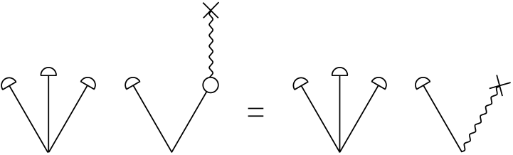
Figure 2: Trivially vanishing leading order. The three fermionic zero modes coming together saturate the operator ${\cal O}_{\mu}^{\,i\beta}$. The other two external legs correspond (on the l.h.s.) to the operator $\lambda\lambda$ or (on the r.h.s.) to its leading-order SUSY variation. In all figures, the indicated equalities hold after antisymmetrization (see fig. 4).

Like eq. (3.19), eq. (3.23) is an off-shell relation in which only the classical equation of motion is used. The fermion propagator emanating from $\partial_{\mu}S_{\mu}^{(0)}$ ends on any one of the five $\lambda$’s in the operator ${\cal O}$. The other four $\lambda$’s are saturated by zero modes. We next eliminate this fermionic propagator using eq. (3.7). Only the delta-function from eq. (3.7) contributes to $\left\langle\delta_{\alpha}{\cal O}\right\rangle$. The terms with the projector $P_{F}$ cancel each other by antisymmetry. These steps are depicted in Fig. 2. (See Fig. 1 for our Feynman rules.) To this order, the diagrams contributing to $\left\langle\delta_{\alpha}{\cal O}\right\rangle$ involve the fermionic zero modes and the classical field, and nothing else. As in eq. (3.18), the vanishing result is obtained before the integration over any of the collective coordinates.

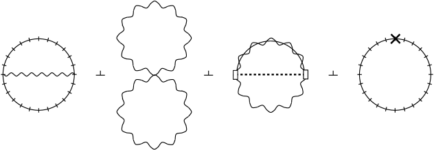
Figure 3: Bubble diagrams. The first and last diagrams contain a sum over boson, fermion and ghost contributions. The third diagram involves the off-diagonal terms of the jacobian eq. (B.13). The last diagram involves (one-loop) self-energy counterterms.

We now turn to the more interesting next order, that corresponding to eq. (3.10). First, there is a set of disconnected diagrams which is trivially zero, since it consists of the same diagrams considered above (Fig. 2) times a sum of bubble diagrams. (The bubble diagrams (Fig. 3) were discussed in detail in ref. [2]. Note that, besides the familiar two-loop diagrams, Fig. 3 contains a one-loop diagram coming from the off-diagonal terms of the jacobian (B.13) or, equivalently, from the interaction term on the last row of eq. (B.38). This is the only place where that term occurs at this order.)

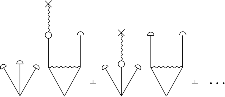
Figure 4: Antisymmetrization. The fermionic projectors (eq. (B.63) or eq. (3.7)) cancel each other after antisymmetrizing with respect to the zero modes and the insertion of $\partial_{\mu}S_{\mu}^{(0)}$.

We next consider Fig. 4. The shown diagrams are related by interchanging the insertion of $\partial_{\mu}S_{\mu}^{(0)}$ with one of the zero modes. Thanks to this antisymmetrization, the fermionic projector terms of eq. (3.7) cancel out. After the application of eq. (3.7), the second diagram gives a contribution to $\delta{\cal O}$.

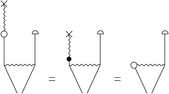
Figure 5: A diagram where $\partial_{\mu}S_{\mu}^{(0)}$ is connected to a fermionic interaction vertex. Here and in the following figures, those external legs which are simply saturated by fermionic zero modes are not shown. As before, the equalities hold after antisymmetrization (including those zero modes which are not shown here, see Fig. 4). The filled circle (here in the middle diagram) indicates that a bosonic field is attached to a fermionic leg of a vertex. The index-matching differential operators (or matrices) can be read off from the appropriate terms in eq. (3.22). On the r.h.s. this is traded with an insertion of eq. (3.25). These diagrams contain a loop (the almost-closed triangle) provided the two external legs are at the same spacetime point.

In the first diagram of Fig. 4, the propagator emanating from $\partial_{\mu}S_{\mu}^{(0)}$ is attached to a fermionic interaction vertex. On the l.h.s. of Fig. 5 we show only the connected part of this diagram containing $\partial_{\mu}S_{\mu}^{(0)}$. Now, the terms in eq. (3.19) which are linear in both the fermion and the boson fields read

$$\partial_{\mu}S_{\mu}^{(1)}=\hat{\beta}^{\dagger}{\buildrel\leftarrow\over{L}}_{B}\,\Gamma\hat{\Psi}+\overline{\delta\Psi}{}^{(1)}{\buildrel\rightarrow\over{\!L}}_{\!F}\,\hat{\Psi}+\overline{\delta\Psi}{}^{(0)}{\cal S}_{F}\,.$$ (3.24)

After the application of eq. (3.7), the l.h.s. of Fig. 5 gives rise to an insertion of (minus the integral of) the last term in eq. (3.24) (middle Fig. 5). Using eq. (3.18), the latter is traded with an insertion of the first two terms on the r.h.s. of eq. (3.24). Explicitly, this insertion is

$$\raisebox{0.0pt}{\Large\boldmath$($}\Gamma\hat{\Psi}\raisebox{0.0pt}{\Large\boldmath$|$}L_{B}\raisebox{0.0pt}{\Large\boldmath$|$}\hat{\beta}\raisebox{0.0pt}{\Large\boldmath$)$}+\raisebox{0.0pt}{\Large\boldmath$($}\delta\Psi^{(1)}\raisebox{0.0pt}{\Large\boldmath$|$}L_{F}\raisebox{0.0pt}{\Large\boldmath$|$}\hat{\Psi}\raisebox{0.0pt}{\Large\boldmath$)$}\,.$$ (3.25)

This step is depicted on the r.h.s. of Fig. 5. (Eq. (3.25) coincides with eq. (C.2) up to the replacement $\delta\Psi\to\delta\Psi^{(1)}$.)

We now apply eqs. (3.8) and (3.7) to the diagram containing insertion (3.25). The terms with the fermionic projector cancel by antisymmetry as before. All other terms are shown in Fig. 6. The last diagram, which involves a longitudinal projector, will be discussed later. The first diagram on the r.h.s. of Fig. 6 is a contribution to $\delta{\cal O}$. (This contribution is a tree or a one-loop diagram, depending on whether the two external legs correspond to different spacetime points or to the same one.) The second diagram vanishes by the same Fiertz rearrangement used in proving the SUSY invariance of the action. (Here we are ignoring the need for regularization, see the next subsection).

The third diagram on the r.h.s. of Fig. 6 is a contribution to the r.h.s. of eq. (3.10). The bosonic zero mode $b_{;n}$ at the upper-left corner of the triangle, the $\bar{\lambda}^{{\buildrel{\raisebox{-1.42262pt}{\large.}}\over{\alpha}}}$ at the same spacetime point and the thick dashed line representing $C_{0}^{-1}$, together form the leading order of $\delta_{\alpha}\zeta_{n}$. The other bosonic zero mode is attached to a fermion line emanating from a fermionic zero mode. Denoting the zero mode by $\chi^{F0}$, this part of the diagram gives the $\zeta_{n}$-derivative $\chi^{F0}_{;n}=-G_{F}\,(L_{F})_{;n}\,\chi^{F0}$.

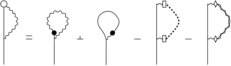
Figure 7: Another diagram with an insertion of eq. (3.25). Again, the second diagram on the r.h.s. vanishes after a Fiertz rearrangement, the third diagram is a contribution to the $\rho$-derivative of $\big{\langle}(\delta_{\alpha}\,\rho)\,\,{\cal O}_{\mu}^{\,i\beta}(0)\,\,\lambda\lambda(y)\big{\rangle}_{\!\rho}$, and the last diagram cancels against other diagrams by gauge invariance.

We now consider two more diagrams with insertion (3.25). The third diagram on the r.h.s. of Fig. 7 gives the $\zeta_{n}$-derivative of the fermionic propagator emanating from $\delta\zeta_{n}$. Fig. 8 contains a one-loop tadpole which is actually zero in SYM. In general, the third diagram on the r.h.s. of Fig. 8 gives the $\zeta_{n}$-derivative of the (logarithm of the) functional determinants.

Let us consider separately the boson, fermion and ghost contributions in the second diagram on the r.h.s. of Fig. 8. The fermion-loop contribution is by itself zero after a Fiertz rearrangement. The ghost-loop diagram will be considered later. For the sum of the remaining one-(bosonic)-loop diagram, plus the first diagram on the r.h.s. of Fig. 7, we use

$$\partial_{\mu}S_{\mu}^{(2)}={\cal S}^{(3,B)}_{\scriptscriptstyle\tilde{I}\tilde{J}\tilde{K}}(b)\;\hat{\beta}_{\scriptscriptstyle\tilde{I}}\hat{\beta}_{\scriptscriptstyle\tilde{J}}\Gamma_{\scriptscriptstyle\tilde{K}\tilde{L}}\hat{\Psi}_{\scriptscriptstyle\tilde{L}}+\overline{\delta\Psi}{}^{(2)}{\buildrel\rightarrow\over{\!L}}_{\!F}\,\hat{\Psi}+\overline{\delta\Psi}{}^{(1)}{\cal S}_{F}\,.$$ (3.26)

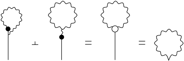
Figure 9: The diagram on the r.h.s. is $\delta\lambda^{(2)}$ (which makes a contribution to $\delta{\cal O}$). The first diagram on the l.h.s. is from Fig. 7, and the second one from Fig. 8.

This allows us to trade the two bosonic-loop diagrams with a single diagram containing an insertion of $\overline{\delta\Psi}{}^{(2)}{\buildrel\rightarrow\over{\!L}}_{\!F}\,\hat{\Psi}$. Using eq. (3.7) once more, we obtain the contribution(s) to $\delta{\cal O}$ coming from $\delta\lambda^{(2)}$ (Fig. 9).

Another type of diagrams with insertion (3.25) is obtained by attaching the bosonic propagator to a quantum gauge field coming from a covariant derivative (cf. eq. (3.12)). One obtains two contributions to $\delta{\cal O}$ and a contribution to the r.h.s. of eq. (3.10), in which the classical field in the background covariant derivative is differentiated with respect to $\zeta_{n}$ (Fig. 10).

We next attach the bosonic propagator from insertion (3.25) to a vertex coming from the expansion of the jacobian (Fig. 11). The second term on the r.h.s. of Fig. 11 gives the $\zeta_{n}$-derivative of the bosonic zero mode contained in $\delta\zeta_{n}$ itself.

The third diagram on the r.h.s. of Fig. 11 gives the $\zeta_{n}$-derivative of $\,\log{\rm det}^{1\over 2}C_{0}$. Particularly relevant for eq. (3.10) are $\rho$-derivatives. As explained earlier, the $\rho$-dependence of ${\rm det}\,C_{0}$ comes from the entries related to the three isospin zero modes. In the matrix $C_{1}$ (eq. (B.14b)), the isospin-isospin entries $(C_{1})_{a^{\prime}c^{\prime}}$ involve the integral of $g\epsilon_{abc}\,\tilde{\omega}^{b}_{c^{\prime}}\,a^{c}_{\mu,a^{\prime}}$ (cf. eq. (3.3)). After taking the product with $\partial a^{a}_{\mu}/\partial\rho$, the result can be written as $ig\,{\rm tr}\,a_{\mu,a^{\prime}}[\tilde{\omega}_{c^{\prime}}\,,\,\partial a_{\mu}/\partial\rho]$. This yields the $\rho$-derivative of ${\rm det}^{1\over 2}C_{0}$, since

$${\partial\over\partial\rho}\,a_{\mu,c^{\prime}}={\partial\over\partial\rho}\,D_{\mu}\,\tilde{\omega}_{c^{\prime}}=-ig\left[{\partial a_{\mu}\over\partial\rho},\tilde{\omega}_{c^{\prime}}\right]+D_{\mu}\,{\partial\tilde{\omega}_{c^{\prime}}\over\partial\rho}\,.$$ (3.27)

The contribution of the last term is zero after integration by parts (which is allowed since $\partial\tilde{\omega}_{c^{\prime}}/\partial\rho$ vanishes rapidly enough at infinity) using $D_{\mu}\,a_{\mu,a^{\prime}}=0$. (The above is an example of the commutator formulae of appendix B.3.)

Last we discuss all diagrams with the longitudinal projector. Compare the last two diagrams in Fig. 6. These diagrams have the same topology, but the meaning of the various elements is different. Recalling the spectral decomposition of the ghost propagator, the analog of the zero mode $b_{;n}$ is now $\Omega^{a}c^{a}_{p}$ where $c^{a}_{p}$ is a ghost eigenstate (see below eq. (3.8), and Appendix B.4). Similarly, the corresponding inverse eigenvalue (associated with the ghost propagator) is the analog of $C_{0}^{-1}$ (the thick dashed line). Thus, those elements which constitute $\delta\zeta_{n}$ in the third diagram, correspond in the last diagram to $\delta\omega_{p}=\mbox{\large\boldmath$($}c^{a}_{p}\mbox{\large\boldmath$|$}\delta\omega^{a}\mbox{\large\boldmath$)$}$ (both to leading order).

Similarly to what we did with the bosonic modes $b_{;n}$, the insertion of $\Omega^{a}c^{a}_{p}$ on a fermion line can be traded with a local gauge transformation with parameter $c^{a}_{p}$, acting on the field(s) at the end(s) of the line. The sum of the resulting diagrams, where the gauge transformation acts on the fields of ${\cal O}$, vanish by gauge invariance of ${\cal O}$. In addition there are diagrams that vanish thanks to gauge invariance of the semi-classical jacobian, or of $\delta\omega_{p}$ itself. One last piece is provided by the ghost-loop diagram that has remained from the second term on the r.h.s. of Fig. 8. It is recognized as a contribution to the gauge transformation of the product $c^{a}_{p}\,{\buildrel\leftarrow\over{\Omega}}{}^{\dagger a}\,\Gamma\hat{\Psi}$ occurring in $\delta\omega_{p}$.

The above completes the diagrammatic analysis of eq. (3.10), except for counterterm diagrams. These will be discussed in the next subsection.

3.3. One-loop renormalization

Several types of loop diagrams occur in the calculation of eq. (3.10), and the corresponding divergences are renormalized by counterterms. In this subsection we complete the proof of eq. (3.10), assuming that renormalized perturbation theory is supersymmetric. (This statement means that the perturbative S-matrix is supersymmetric, and that perturbative matrix elements of composite operators fall into supermultiplets.) We assume that the counterterms were constructed using the background field method [13]. For definiteness we will refer to dimensional regularization, but the discussion generalizes to any other consistent regularization as well. As mentioned earlier, the below arguments are actually sufficient to prove eq. (1.3) after renormalization, whenever its r.h.s. consists of tree diagrams only.

As explained in the previous subsections, the two-loop bubble diagrams that occur on the l.h.s. of eq. (3.10) are multiplied by zero. Thus, we need not concern ourselves here with the corresponding counterterm diagrams. (There are delicate points in the renormalization of the bubble diagrams, see ref. [2]; these will become relevant at higher orders.)

We next consider the ghost-loop diagram contained in the second term on the r.h.s. of Fig. 8, and all the (loop) diagrams with the longitudinal projector $P^{\parallel}$. As discussed in the previous subsection, the sum of these diagrams is zero by gauge invariance. Since (background) gauge invariance is preserved by the regularization, this cancelation continues to hold.

The remaining divergences arise from one-loop diagrams containing boson or fermion propagators, and no ghost propagator. Renormalization of these diagrams requires us to face two obstacles. First, dimensional regularization treats a loop as a single entity. Equations like eq. (B.63),  (3.8) or (3.7) do not hold for $d-4\neq 0$. We must therefore replace these equations by ones that hold for arbitrary $d$. The second (related) complication is that SUSY, as expressed by eq. (3.19), is broken by terms proportional to $d-4$.

We now explain how dimensional regularization is applied to an instanton-sector diagram. First, repeating $n$ times the recursion relation for the generic fermion propagator $G_{F}$, eq. (B.67), we obtain

$$G_{F}=\left(1-P_{F}^{\rm exact}\right)G_{F}^{\rm vac}\sum_{k=0}^{n}\left(-\tilde{V}_{F}G_{F}^{\rm vac}\right)^{k}+G_{F}\left(-\tilde{V}_{F}G_{F}^{\rm vac}\right)^{n+1}\,.$$ (3.28)

(The superscript “vac” denotes free-field quantities, and $\tilde{V}_{F}=L_{F}-L_{F}^{\rm vac}$. Notice the terms with the projector $P_{F}^{\rm exact}$, which “cut open” any loop containing $G_{F}$.) We now take $n$ (finite and) high enough, such that any loop containing $L_{F}$ times the last term in eq. (3.28) will be finite. Eq. (B.63) may be applied to the last term, and the result is

$$L_{F}\,G_{F}=\left(L_{F}^{\rm vac}+\tilde{V}_{F}\right)G_{F}^{\rm vac}\sum_{k=0}^{n-1}\left(-\tilde{V}_{F}G_{F}^{\rm vac}\right)^{k}+L_{F}^{\rm vac}G_{F}^{\rm vac}\left(-\tilde{V}_{F}G_{F}^{\rm vac}\right)^{n}-P_{F}^{\rm exact}\,.$$ (3.29)

We have used (see below eq. (B.67))

$$P_{F}^{\rm exact}\left(-\tilde{V}_{F}G_{F}^{\rm vac}\right)^{n}=P_{F}^{\rm exact}\,.$$ (3.30)

Eqs. (3.28) and (3.29) provide the key for regularization. Comparing eq. (3.29) with eq. (B.63), we see that the term with $P_{F}^{\rm exact}$ has been separated out explicitly. The remaining terms, which replace the delta-function in eq. (B.63), are identical to what one would have found in a standard perturbative expansion. Any (loop) diagram containing (only) these perturbative-expansion terms is amenable to dimensional (or any other) regularization. (If $L_{F}^{\rm vac}\,G_{F}^{\rm vac}(x,y)=\delta^{4}(x-y)$ is true in the regularized theory, then eq. (3.29) reduces to eq. (B.63).)

(In SYM, the bosonic and fermionic propagators in the instanton sector obey eqs. (3.8) and (3.7) respectively, and the above analysis is applicable to both of them. In the bosonic equivalent of eq. (3.29), $P_{F}^{\rm exact}$ is replaced by $P_{B}+P^{\parallel}$. The ghost propagator contained in the longitudinal projector (cf. eq. (B.60)) obeys the standard recursion relation (B.65). In the most general case $G_{B}$ is defined by eq. (B.53). The last term in this equation cuts open any loop since (like projectors) it involves a localized source. As for $\hat{G}_{B}$, it is convenient (cf. Appendix B.6) to consider first $\xi\neq 0$. Then $\hat{G}_{B}$ obeys eq. (B.47) and the standard recursion relation (B.65). Using eq. (B.58), all term involving $1/\xi$ may be replaced by expressions that have a smooth $\xi\to 0$ limit.)

Let us now examine, in comparison, the background-field fermion propagator in the vacuum sector. This propagator obeys the standard recursion relation (B.65) and, therefore, identities analogous to eqs. (3.28) and (3.29) but without projector terms. Similarly, the vacuum-sector identities for the background-field transverse boson propagator contain the longitudinal projector, but no analog of the projector $P_{B}$.

When the manipulations based on eq. (3.19) are carried out in the vacuum sector, all (finite) violations of SUSY that survive the removal of the regularization can be canceled by an appropriate (non-supersymmetric) set of counterterms [14]. The cancelation of SUSY violations arising from the loop regularization continues to hold in the instanton sector. As a result, whenever $L_{B}\,G_{B}$ or $L_{F}\,G_{F}$ arise inside some (amputated) one-loop diagram (from the application of eq. (3.19)) this yields a renormalized diagrammatic identity in the instanton sector which differs from the corresponding one in the vacuum sector precisely by the projector terms $P_{F}^{\rm exact}$ and $P_{B}$. As shown in the previous subsection, all diagrams with an insertion of $P_{F}^{\rm exact}$ cancel by antisymmetry, while those containing $P_{B}$ combine with diagrams that involve the functional jacobian to form the total $\zeta_{n}$- (and in particular $\rho$-) derivatives.

We now explain how the last statement works in practice. Consider first the loop diagram on the l.h.s. of Fig. 7, which originates from the self-energy diagram in Fig. 12(a). There is a corresponding counterterm diagram, shown in Fig. 12(b). (As mentioned earlier, the sum of one-loop tadpoles in Fig. 8 is zero in SYM.) Now, the r.h.s. of Figs. 7 and 8 also contains loop diagrams, to which we have to apply eq. (3.26), cf. Fig. 9. That equation, which is an expression of SUSY of the action, is broken in dimensional regularization by an amount proportional to $d-4$. When multiplied by $(d-4)^{-1}$ coming from the loop divergence, a (finite) explicit breaking of SUSY may result. This explicit breaking is canceled, however, by an appropriate non-supersymmetric set of counterterms. Consequently, the renormalized equalities represented by figs. 7, 8 and 9 hold after adding the counterterm diagram.

A second set of one-loop diagrams can be found in Figs. 4, 5 and 6 (provided both of the external legs go to the same spacetime point). The divergences in these figures correspond to the composite operators $\lambda\lambda$ or ${\cal O}_{\mu}^{\,i\beta}$ (eq. (3.11)), or to their SUSY variations. For example, $\delta(\lambda\lambda)=(i/\sqrt{2})\,\sigma_{\mu\nu}F_{\mu\nu}\,\lambda$. However, in general

$$\delta[\lambda\lambda]^{(1)}\neq(i/\sqrt{2})[\sigma_{\mu\nu}F_{\mu\nu}\,\lambda]^{(1)}\,,$$ (3.31)

where $[\cdots]^{(1)}$ is the corresponding one-loop counterterm. The l.h.s. of inequality (3.31) is shown in Fig. 13(a), while its r.h.s. is Fig. 13(b). (The counterterms are normally $O(g^{2})$, but when they involve a classical field they become $O(g)$.) Again, the counterterms are designed to compensate for any discrepancy that may have arisen from the loop regularization. With the counterterm diagrams added, the equalities of Figs. 4, 5 and 6 hold after renormalization. Finally, the loops of Fig. 10 are treated in a similar manner. We leave it for the reader to work out the corresponding counterterm diagrams. This completes the proof of eq. (3.10).

At higher orders, the renormalization of eq. (3.10) is more complicated, because one must deal with the divergences arising from the coupling between the discrete- and the continuous-index parts of the jacobian. This problem was addressed in ref. [2]. A related problem is that one must deal with the divergences of $\delta\rho$. In subsection 3.6 below we use a renormalization-group argument to determine the next-order logarithmic corrections to eq. (3.10).

3.4. SUSY theories with matter

It is easy to generalize eq. (3.10) to SU(2) SQCD. Let the number of flavors be $N_{f}$. (By convention, for SU(2) each flavor corresponds to two chiral supermultiplets in the fundamental representation. Each (massless) Weyl-fermion field has one zero mode.) One has

$$\left\langle\delta_{\alpha}\,\,{\cal O}_{\mu}^{\,i\beta}(0)\,\,\lambda\lambda(y)\,\,\prod_{k=1}^{N_{f}}\widetilde{\psi_{k}\psi_{k}}(0)\right\rangle=-{2^{12.5}3\pi^{2}\Lambda_{1}^{6-N_{f}}\over 7g^{7}}\,{\bar{\eta}_{i\mu\tau}[\sigma_{\nu}\,\bar{\sigma}_{\tau}]_{\alpha}^{\,\beta}\,y_{\nu}\over(y^{2})^{3}}\,,$$ (3.32)

where

$$\widetilde{\psi_{k}\psi_{k}}(q)=\int d^{4}x\,e^{iqx}\,\psi_{k}\psi_{k}(x)\,.$$ (3.33)

We have assumed $y^{2}m^{2}\ll 1$ where $m$ is a generic matter-field mass. This implies that only the zero modes contribute in eq. (3.33). As shown in subsection 4.1 below, both eq. (3.10) and eq. (3.32) cannot be modified by subtractions and, hence, constitute a supersymmetry anomaly. Eq. (3.32) reflects a general feature, namely, the anomalous term may be a polynomial in some of the external momenta (here the polynomial in $q_{\mu}$ reduces to a constant).

For SU(N), One should replace ${\cal O}_{\mu}^{\,i\beta}$ by an operator whose generic structure is $\lambda(D_{\mu}\,\lambda)(D^{2}\lambda)(\lambda\lambda)^{N-2}$. The generalization of eq. (3.10) will have on its r.h.s. $c_{N}\,g^{1-4N}\,\Lambda_{1}^{3N-N_{f}}$ times similar spacetime dependent factors. We have not worked out the numerical constant $c_{N}$.

3.5. Local form of the anomaly

The local version of eq. (1.3) is obtained by applying the SUSY variation of the fields only at the point $x=z$. To this end, one multiplies the l.h.s. of eqs. (2.2) and (2.5) by $\delta^{4}(x-z)$. One can now repeat the construction of Sec. 2. An easy way to read the local variations from those of Sec. 2.1 is to associate the $\delta^{4}(x-z)$ factor with the matrix $\Gamma$. Whenever $\Gamma\hat{\Psi}$ occurs inside some integral, it is replaced by the corresponding integrand at $x=z$. For the local variations of the collective coordinates one obtains

$$\delta\zeta_{m}(z)=C^{-1}_{mn}\left\{b_{;n}^{\dagger}(z)\,\Gamma\hat{\Psi}(z)+ig\int d^{4}x\,b_{;n}^{\dagger}(x)\,T^{a}\hat{\beta}(x)\,\delta\omega^{a}(x;z)\right\}\,,$$ (3.34)

where

$$\delta\omega^{a}(x;z) = {\cal F}^{-1}_{ab}(x,z)\,\Omega^{b\dagger}(z)\,\Gamma\hat{\Psi}(z)$$ (3.35)

$$+ig\int d^{4}y\,{\cal F}^{-1}_{ab}(x,y)\,b_{;m}^{\dagger}(y)\,T^{b}\hat{\beta}(y)\;C^{-1}_{mn}\;b_{;n}^{\dagger}(z)\,\Gamma\hat{\Psi}(z)\,.$$

The variation of the measure is zero as before, and the local form of eq. (1.3) reads

$$\partial_{\mu}\left\langle\hat{S}_{\mu}(z)\,{\cal O}\right\rangle=\mbox{contact terms}-\int d^{n}\zeta\;{\partial\over\partial\zeta_{n}}\left(e^{-S_{\rm cl}-W_{1}-W_{2}}\,\left\langle\delta\zeta_{n}(z)\,{\cal O}\right\rangle_{\!\zeta}\right)\,,$$ (3.36)

where the contact terms are the expected variations of the (multi)local operator ${\cal O}$. The last term in eq. (3.36) is, by definition, a matrix element of the operator $\partial_{\mu}\hat{S}_{\mu}(z)$. Another way of reaching these results is to keep track of the diagrammatic identities of Sec. 3.2, but now without performing the integral in eq. (3.18). For the local form of eq. (3.10) we find

$$\partial_{\nu}\left\langle\hat{S}_{\nu\alpha}(z)\,\,{\cal O}_{\mu}^{\,i\beta}(0)\,\,\lambda\lambda(y)\right\rangle=\mbox{contact terms}-\left\langle\partial_{\nu}\hat{S}_{\nu\alpha}(z)\,\,{\cal O}_{\mu}^{\,i\beta}(0)\,\,\lambda\lambda(y)\right\rangle\,,$$ (3.37)

where the matrix element of $\partial_{\nu}\hat{S}_{\nu\alpha}(z)$ is

$$\left\langle\partial_{\nu}\hat{S}_{\nu\alpha}(z)\,\,{\cal O}_{\mu}^{\,i\beta}(0)\,\,\lambda\lambda(y)\right\rangle = -2^{10}\pi^{6}g^{-8}\Lambda_{1}^{6}\,\lim_{\rho\to 0}\,\rho^{3}\,\left\langle(\delta_{\alpha}\,\rho(z))\,\,{\cal O}_{\mu}^{\,i\beta}(0)\,\,\lambda\lambda(y)\right\rangle_{\!\rho}$$ (3.38)

$$=\hskip 56.9055pt {2^{11.5}\Lambda_{1}^{6}\over 7g^{7}}\,{\eta_{b\rho\nu}\,z_{\nu}\over(z^{2})^{2}}\,{(y-z)_{\kappa}\over((y-z)^{2})^{2}}\,{\eta_{b\lambda\sigma}\,y_{\sigma}\over(y^{2})^{2}}\,\bar{\eta}_{i\mu\tau}[\sigma_{\rho}\,\bar{\sigma}_{\kappa}\,\sigma_{\lambda}\,\bar{\sigma}_{\tau}]_{\alpha}^{\,\beta}\,.$$

Eq. (3.38) is consistent with locality of $\partial_{\nu}\hat{S}_{\nu\alpha}(z)$. As expected, one recovers the r.h.s. of eq. (3.10) by integrating over $z$ in eq. (3.38).

3.6. Renormalization group considerations

At the next-to-leading order, the Hilbert-space surface term on the last row of eq. (3.13) may pick up logarithmic corrections. Depending on the power of $\log\rho$, the result of the $\rho\to 0$ limit could blow up, remain finite, or vanish.

In fact, the logarithmic corrections may be either $\log\rho$ or $\log y^{2}$. This is because the limit in eq. (3.13) is not uniform: while the effective range of the $x_{0}$-integration scales to zero with $\rho$, the distance scale $y^{2}$ is kept fixed. Taking this delicate point into consideration, we now give a renormalization-group (RG) argument that the $\log\rho$ factors arising from $\delta_{\alpha}\rho$ and ${\cal O}_{\mu}^{\,i\beta}$ should cancel those arising from two-loop bubble diagrams.

Given a renormalization point $\mu$, we rewrite eq. (3.10) to one higher order as

$$g^{5}(\mu)\left\langle\delta_{\alpha}\,\,{\cal O}_{\mu}^{\,i\beta}(0)\,\,\lambda\lambda(y)\right\rangle=-\Lambda_{2}^{6}\,g^{2}(\mu)\,{2^{12.5}3\pi^{2}\bar{\eta}_{i\mu\tau}[\sigma_{\nu}\,\bar{\sigma}_{\tau}]_{\alpha}^{\,\beta}\,y_{\nu}\over 7(y^{2})^{3}}\,(1+{\rm logs})\,.$$ (3.39)

The two-loop RG-invariant scale is

$$\Lambda_{2}^{6}=\mu^{6}\,g^{-4}(\mu)\,\exp(-8\pi^{2}/g^{2}(\mu))\,.$$ (3.40)

The reason for including the $g^{5}(\mu)$ factor in eq. (3.39) is as follows. First, the operator $\delta_{\alpha}\rho$ is RG-invariant because the collective coordinate $\rho$ is independent of the renormalization point $\mu$, and the SUSY variation $\delta_{\alpha}$ respects RG-invariance. More generally, the basic building blocks of RG-invariant operators are $gF_{\mu\nu}$ and $g\lambda$ (or $g\bar{\lambda}$). We have therefore multiplied ${\cal O}_{\mu}^{\,i\beta}(0)$ and $\lambda\lambda(y)$ by appropriate powers of $g(\mu)$.

We now analyze the expected $\log\rho$ corrections, starting with the contribution of the two-loop bubble diagrams [2]. The semi-classical instanton measure (3.9) involves the product $\Lambda_{2}^{6}\,g^{-4}(\mu)$. RG invariance requires that, for size-$\rho$ instantons, the logarithms arising from the bubble diagrams should turn this product into $\Lambda_{2}^{6}\,g^{-4}(\rho^{-1})$. Next consider the operator $\delta_{\alpha}\rho$. As can be seen from eqs. (3.14) and (3.15), the coupling constant explicitly contained in $\delta_{\alpha}\rho$ is associated with the classical field. The logarithmic corrections to $\delta_{\alpha}\rho$ should modify that $g(\mu)$ to $g(\rho^{-1})$.

Finally, RG invariance of $g^{3}{\cal O}_{\mu}^{\,i\beta}$ means that the exponential involving its anomalous dimension, $\exp[\int_{g(\mu)}^{g(\rho^{-1})}dg^{\prime}\,\gamma_{\cal O}(g^{\prime})/\beta(g^{\prime})]$, must be proportional to $g^{3}(\rho^{-1})/g^{3}(\mu)$. In other words, the renormalization of ${\cal O}_{\mu}^{\,i\beta}$ provides $\log\rho$ factors which are just enough to turn $g^{3}(\mu)$ into $g^{3}(\rho^{-1})$. Putting together the expected $\log\rho$ factors arising from all sources we find that they cancel each other. (Of course, it is important to confirm this conclusion by a direct next-order calculation.) Moreover, all higher-order corrections to both $\gamma_{\cal O}(g)$ and $\beta(g)$ cannot give rise to $\log\rho$ terms in the solution of the RG equation.

Finally, if the scale $y^{2}$ is varied, one expects the renormalization of $\lambda\lambda(y)$ to generate $\log y^{2}$ factors that turn $g^{2}(\mu)$ into $g^{2}(|y|^{-1})$. We thus expect the next-order result to be

$$g^{5}(\mu)\left\langle\delta_{\alpha}\,\,{\cal O}_{\mu}^{\,i\beta}(0)\,\,\lambda\lambda(y)\right\rangle=-\Lambda_{2}^{6}\,g^{2}(|y|^{-1})\,{2^{12.5}3\pi^{2}\bar{\eta}_{i\mu\tau}[\sigma_{\nu}\,\bar{\sigma}_{\tau}]_{\alpha}^{\,\beta}\,y_{\nu}\over 7(y^{2})^{3}}\,.$$ (3.41)

Assume now that $y^{6}\Lambda_{1}^{6}\ll 1$. While SYM is confining, the contributions of sectors with additional instanton-antiinstanton pairs should be damped compared to eq. (3.10) (or eq. (3.41)) by extra powers of $y^{6}\Lambda_{1}^{6}$. What we are calculating is thus the leading-order result in an expansion in the physical parameter $y^{6}\Lambda_{1}^{6}=\exp(-8\pi^{2}/g^{2}(y^{-1}))$.

4.  The $\rho\to 0$  limit

The limit of a vanishing-size instanton, $\rho\to 0$, may be singular in correlation functions that involve operators of sufficiently high dimension. In this section we investigate several aspects of this limit. Our main result (subsection 4.1) is that the anomalous Ward identity eq. (3.10) cannot be modified by non-perturbative subtractions and, hence, constitutes a supersymmetry anomaly. In subsection 4.2 we discuss point splitting, and explain why it does not regularize the operator ${\cal O}_{\mu}^{\,i\beta}$ occurring in eq. (3.10). In subsection 4.3 we describe an ambiguity that arises in a case where point splitting can be used and comment on its implications. In subsection 4.4 we explain how the anomaly should arise on the lattice.

4.1. Non-perturbative subtractions

In this subsection we first examine separately the two correlators $\big{\langle}(\delta_{\alpha}\,{\cal O}_{\mu}^{\,i\beta})\,\,\lambda\lambda\big{\rangle}$ and $\big{\langle}{\cal O}_{\mu}^{\,i\beta}\,\,(\delta_{\alpha}\,\lambda\lambda)\big{\rangle}$, whose difference is eq. (3.10). We show that the corresponding $\rho$-integrals are convergent in the limit $\rho\to 0$.

For comparison, we next consider another Ward identity where the corresponding integrals are divergent for $\rho\to 0$. In that case non-perturbative subtractions are needed, and may in fact be used to recover SUSY. Having worked out this explicit example, we list the general properties of non-perturbative subtractions. It then easily follows that eq. (3.10) cannot be modified by any non-perturbative subtraction.

In subsection 3.1 we have computed the correlation function $\big{\langle}(\delta_{\alpha}\,\rho)\,\,{\cal O}_{\mu}^{\,i\beta}(0)\,\,\lambda\lambda(y)\big{\rangle}_{\!\rho}$ (eq. (3.13)) in the limit $\rho\to 0$. Let us now generalize the calculation to any $\rho$. The operator product on the l.h.s. of eq. (3.16) may be written as $2\lambda^{SC}(y;{\buildrel{\raisebox{-1.42262pt}{\large.}}\over{\alpha}})\,\lambda^{{\rm ind}}(y;\alpha)$ where

$$\bar{\sigma}_{\mu}^{{\buildrel{\raisebox{-1.42262pt}{\large.}}\over{\beta}}\beta}D_{\mu}^{ab}\,\lambda^{{\rm ind,}\,b}_{\beta}(\alpha)={g^{2}\,\bar{\sigma}_{\mu}^{{\buildrel{\raisebox{-1.42262pt}{\large.}}\over{\beta}}\alpha}\over 2^{4.5}\pi^{2}}\,{\partial a^{a}_{\mu}\over\partial\rho}\,.$$ (4.1)

In a regular gauge, the solution is

$$\lambda^{{\rm ind,}\,b}_{\beta}(y;\alpha)={\rho\,g\over 2^{3.5}i\pi^{2}}\,{\sigma^{b\alpha}_{\beta}\over(y-x_{0})^{2}+\rho^{2}}\,.$$ (4.2)

Performing the $x_{0}$-integration we find (ignoring irrelevant constants)

$$\rho^{3}\left\langle(\delta_{\alpha}\,\rho)\,\,{\cal O}_{\mu}^{\,i\beta}(0)\,\,\lambda\lambda(y)\right\rangle_{\!\rho}\propto{\Lambda_{1}^{6}\,\bar{\eta}_{i\mu\tau}[\sigma_{\nu}\,\bar{\sigma}_{\tau}]_{\alpha}^{\,\beta}\over g^{7}}\,{y_{\nu}\,h(\rho^{2}/y^{2})\over(y^{2})^{3}}\,,$$ (4.3)

where $h(s)$ can be represented as a Feynman-parameters integral (see Appendix E of ref. [8]) and

$$h(s)=\left\{\begin{array}[]{ll}1+h_{1}\,s+h_{2}\,s^{2}+\cdots,&\quad s\ll 1\,,\\ h_{-3}\,s^{-3}+h_{-4}\,s^{-4}+\cdots,&\quad s\gg 1\,.\end{array}\right.$$ (4.4)

Eq. (3.10) thus involves the integral

$${y_{\nu}\over(y^{2})^{3}}\int d\rho\,{\partial\over\partial\rho}\,h(\rho^{2}/y^{2})\,.$$ (4.5)

This integral is convergent, with the main contribution to it arising from $\rho^{2}\sim y^{2}$. For small $\rho^{2}/y^{2}$, the integrand in (4.5) behaves like $\rho y/(y^{2})^{4}$.

We now turn to the correlators $\big{\langle}(\delta_{\alpha}\,{\cal O}_{\mu}^{\,i\beta}(0))\,\,\lambda\lambda(y)\big{\rangle}$ and $\big{\langle}{\cal O}_{\mu}^{\,i\beta}(0)\,\,(\delta_{\alpha}\,\lambda\lambda(y))\big{\rangle}$. We claim that both the small- and the large-$\rho$ behavior of the corresponding integrals is the same as in eq. (4.5) above. In the limit $\rho\to\infty$ this can be established simply on dimensional grounds. Turning to the $\rho\to 0$ limit we first examine $\big{\langle}(\delta_{\alpha}\,{\cal O}_{\mu}^{\,i\beta}(0))\,\,\lambda\lambda(y)\big{\rangle}$. At tree level, if the product of zero modes at the point $y$ is $\lambda^{SC}(y)\,\lambda^{SS}(y)$ then the presence of $y/(y^{2})^{4}$ is evident and, on dimensional grounds, implies a $\rho y/(y^{2})^{4}$ behavior of the $\rho$-integrand. Alternatively, if one places both superconformal modes at the point $y$ then the factorized $y$-independent piece, $\int d^{4}x_{0}\,\big{\langle}\delta_{\alpha}\,{\cal O}_{\mu}^{\,i\beta}(0)\big{\rangle}_{x_{0},\rho}$, is zero because the $x_{0}$-integral is odd (compare eq. (3.17)). The first non-zero contribution again goes like $\rho y/(y^{2})^{4}$. At the one-loop level one reaches the same conclusion by examining the (small-$\rho$ behavior of the) fermion propagator in the relevant partial wave. Having established this (large- and) small-$\rho$ behavior of $\big{\langle}(\delta_{\alpha}\,{\cal O}_{\mu}^{\,i\beta}(0))\,\,\lambda\lambda(y)\big{\rangle}$, eqs. (4.3) to (4.5) imply the same behavior for the $\rho$-integrand in $\big{\langle}{\cal O}_{\mu}^{\,i\beta}(0)\,\,(\delta_{\alpha}\,\lambda\lambda(y))\big{\rangle}$. (Reaching this conclusion directly is more difficult: the correlator involves a diagram with a vector-boson propagator connecting the points 0 and $y$, and in an instanton background this propagator decreases very slowly [12]; see, however, ref. [15].)

Before turning to the physical implications of eq. (3.10), we wish to explain in what way things could be different. To this end, we consider another anomalous SUSY Ward identity, which is

$$\left\langle\bar{\delta}_{{\buildrel{\raisebox{-1.42262pt}{\large.}}\over{\alpha}}}\,\,\lambda\lambda F^{3}_{ijk}(0)\,\,\sigma F\lambda_{\alpha}(y)\right\rangle=-\epsilon_{ijk}\,{2^{22.5}\pi^{4}\Lambda_{1}^{6}\over g^{11}(y^{2})^{4}}\,(\sigma_{\mu})_{\alpha{\buildrel{\raisebox{-1.42262pt}{\large.}}\over{\alpha}}}\,y_{\mu}\,,$$ (4.6)

where $\sigma F\lambda_{\alpha}\equiv\sigma^{\mu\nu}_{\alpha\beta}F_{\mu\nu}^{c}\lambda^{c\beta}$ and

$$F^{3}_{ijk}\equiv\epsilon_{abc}F^{a}_{\mu\nu}F^{b}_{\lambda\rho}F^{c}_{\sigma\tau}\bar{\eta}_{i\mu\nu}\bar{\eta}_{j\lambda\rho}\bar{\eta}_{k\sigma\tau}\,.$$ (4.7)

The calculation is similar to subsection 3.1, and is in fact simpler. $\bar{\delta}_{{\buildrel{\raisebox{-1.42262pt}{\large.}}\over{\alpha}}}\rho$ involves a $\lambda$ field, which is saturated by one of the $\lambda^{SC}$ modes, while the other $\lambda^{SC}$ goes to the operator $\sigma F\lambda_{\alpha}$. Note that eq. (4.6) exhibits a $y^{-7}$ fall-off which is faster than the $y^{-5}$ fall-off in eq. (3.10). This kinematic difference will turn out to play an important role.

We now show that the operator $\lambda\lambda F^{3}_{ijk}$ requires a non-perturbative subtraction. Consider the following correlator

$$\left\langle\lambda\lambda F^{3}_{ijk}(0)\,\,\lambda\lambda(y)\right\rangle\sim\epsilon_{ijk}\,{\Lambda_{1}^{6}\over g^{11}(y^{2})^{3}}\int{d\rho\over\rho}\,,$$ (4.8)

where on the r.h.s. we have indicated the small-$\rho$ behavior. The non-perturbative logarithmic divergence at small $\rho$ can be handled as follows. We first restrict the integral to $\bar{\rho}\leq\rho<\infty$ where $0<\bar{\rho}$. A subtracted operator is defined via

$$[\lambda\lambda F^{3}_{ijk}]=\lambda\lambda F^{3}_{ijk}-\epsilon_{ijk}\,c_{3}\,\log(\mu\bar{\rho})\,{\Lambda_{1}^{6}\over g^{11}}\,\bar{\lambda}\bar{\lambda}\,,$$ (4.9)

where $c_{3}$ is a suitable numerical constant. The subtracted operator $[\lambda\lambda F^{3}_{ijk}]$ yields a finite $\bar{\rho}\to 0$ result when substituted into the l.h.s. of eq. (4.8).

Like $\lambda\lambda F^{3}_{ijk}$, the operator $\bar{\delta}_{{\buildrel{\raisebox{-1.42262pt}{\large.}}\over{\alpha}}}\,\lambda\lambda F^{3}_{ijk}$ requires a non-perturbative subtraction too. We now define the renormalized operator as follows

$$[\bar{\delta}_{{\buildrel{\raisebox{-1.42262pt}{\large.}}\over{\alpha}}}\,\lambda\lambda F^{3}_{ijk}]\equiv\bar{\delta}_{{\buildrel{\raisebox{-1.42262pt}{\large.}}\over{\alpha}}}\,[\lambda\lambda F^{3}_{ijk}]+\epsilon_{ijk}\,{2^{21}\pi^{8}\Lambda_{1}^{6}\over 9g^{11}}\,\bar{\delta}_{{\buildrel{\raisebox{-1.42262pt}{\large.}}\over{\alpha}}}\,\bar{\lambda}\bar{\lambda}\,.$$ (4.10)

We have chosen a manifestly non-supersymmetric subtraction. The finite, last term in eq. (4.10) was chosen to cancel the r.h.s. of eq. (4.6). Using the vacuum-sector result

$$\left\langle\bar{\sigma}F\bar{\lambda}_{{\buildrel{\raisebox{-1.42262pt}{\large.}}\over{\alpha}}}(0)\,\,\sigma F\lambda_{\alpha}(y)\right\rangle_{\rm vac}=-{36i\over\pi^{4}(y^{2})^{4}}(\sigma_{\mu})_{\alpha{\buildrel{\raisebox{-1.42262pt}{\large.}}\over{\alpha}}}\,y_{\mu}\,,$$ (4.11)

eq. (4.6) becomes

$$\left\langle[\bar{\delta}_{{\buildrel{\raisebox{-1.42262pt}{\large.}}\over{\alpha}}}\,\lambda\lambda F^{3}_{ijk}(0)]\,\,\sigma F\lambda_{\alpha}(y)+[\lambda\lambda F^{3}_{ijk}(0)]\,\,\bar{\delta}_{{\buildrel{\raisebox{-1.42262pt}{\large.}}\over{\alpha}}}\,\sigma F\lambda_{\alpha}(y)\right\rangle=0\,.$$ (4.12)

Eq. (4.12) means that SUSY has been recovered in the limit $\bar{\rho}\to 0$ after performing the above non-perturbative subtractions. Moreover, by considering additional Ward identities, one can verify that the renormalized operators respect the SUSY algebra. (Recovering the supermultiplet structure of composite operators by suitable subtractions is a reminiscent of the so-called Konishi anomaly [9].)

There are two lessons from the above example. First, when non-perturbative subtractions play a role, there is at least a chance that SUSY will be recovered. The other lesson has to do with the general properties of non-perturbative subtractions. A divergence at $\rho\to 0$ always arises from a kinematic situation where the instanton sits on top of an operator ${\cal O}(x)$ of a sufficiently high dimension. Consider the instanton-sector correlation function $\big{\langle}{\cal O}(x)\prod_{k}{\cal O}_{k}(y_{k})\big{\rangle}$ and assume that a $\rho\to 0$ divergence arises only from the operator ${\cal O}(x)$. The zero modes and the propagators which are functions of $y_{1},y_{2},\ldots,$ become $\rho$-independent in the limit $\rho\to 0$. (More generally, they are expandable in powers of $\rho$; this expansion is used when the leading divergence is stronger than $\log\rho$.)

As a result, the dependence on spacetime points of the $\rho\to 0$ divergence must be that of a vacuum-sector correlation function $\big{\langle}{\cal O}^{\prime}(x)\prod_{k}{\cal O}_{k}(y_{k})\big{\rangle}_{\rm vac}$ involving another operator ${\cal O}^{\prime}(x)$. The operators ${\cal O}(x)$ and ${\cal O}^{\prime}(x)$ must have the same quantum numbers except for their chiral charge, where the mismatch is given by the number of fermionic zero modes. Because of the explicit $\Lambda_{1}^{6}$ factor which appears in instanton-sector correlation functions, the dimension of ${\cal O}^{\prime}$ must be smaller than that of ${\cal O}$ at least by 6. (The difference between the dimensions of ${\cal O}(x)$ and ${\cal O}^{\prime}(x)$ is 6 (for SU(2)) if the divergence is logarithmic; if the divergence goes like some inverse power of $\rho$, the difference is 6 plus that power.)

Previously, we showed that there is no small-$\rho$ divergence in the correlation functions $\big{\langle}(\delta_{\alpha}\,{\cal O}_{\mu}^{\,i\beta}(0))\,\,\lambda\lambda(y)\big{\rangle}$ and $\big{\langle}{\cal O}_{\mu}^{\,i\beta}(0)\,\,(\delta_{\alpha}\,\lambda\lambda(y))\big{\rangle}$. It is now easy to generalize this result, and show that no instanton-sector correlation function can have a $\rho\to 0$ divergence associated with the operators ${\cal O}_{\mu}^{\,i\beta}$ or $\delta_{\alpha}{\cal O}_{\mu}^{\,i\beta}$. If such a divergence were to arise in some correlation function, then from the spacetime dependence of the divergence one could read off what is the necessary non-perturbative subtraction. However, there is no operator that qualifies as a non-perturbative subtraction for ${\cal O}_{\mu}^{\,i\beta}$ or for $\delta_{\alpha}{\cal O}_{\mu}^{\,i\beta}$. The mass dimension of ${\cal O}_{\mu}^{\,i\beta}$ is 7.5. Therefore, for the subtraction one would need an operator whose dimension is $7.5-6=1.5$. Evidently, there is no gauge invariant operator with this dimension. A similar conclusion applies to $\delta_{\alpha}{\cal O}_{\mu}^{\,i\beta}$. Since eq. (3.10) cannot be modified by any non-perturbative subtraction, there is no way to recover that SUSY Ward identity. Hence, eq. (3.10) constitutes a supersymmetry anomaly.

One may wonder how the physical implications of eqs. (3.10) and (4.6) can be so different. Apart from the above mentioned kinematic difference ($y^{-7}$ vs. $y^{-5}$ fall-off), there are two more significant differences between the two Ward identities. In eq. (4.6), only the fermionic zero modes and the classical field occur on both sides. As shown in ref. [7], the collective coordinates and the fermionic zero modes constitute a finite supersymmetric system. One does not expect that SUSY will be violated when these are the only relevant degrees of freedom. On the other hand, in eq. (3.10) the l.h.s. involves one-loop diagrams which are outside the scope of the supersymmetric calculus of ref. [7], and the potential for an anomaly exists.

The other qualitative difference between eqs. (3.10) and (4.6) is in the corresponding local Ward identities. In the case of eq. (4.6), the $\rho\to 0$ limit and the integration over the point $z$, where the SUSY variation is performed, do not commute. Ignoring irrelevant constants, the product $\lambda^{SC}(z)\,\partial a_{\mu}/\partial\rho(z)$ which occurs in $\bar{\delta}_{{\buildrel{\raisebox{-1.42262pt}{\large.}}\over{\alpha}}}\rho(z)$, is $\rho^{2}z^{2}/(z^{2}+\rho^{2})^{4}$. This becomes a delta-function, $\delta^{4}(z)$, in the limit $\rho\to 0$. As a result, the corresponding local matrix element is zero except for $z=0$. When the only violation of the naive Ward identity is of this type, it is natural to associate this effect with a modification of the composite-operator transformation rule, and not with a non-zero $\partial_{\mu}\hat{S}_{\mu}(z)$.

In contrast, the local form of eq. (3.10) (namely Eq. (3.38)) is non-zero for any $z$. Moreover, after the $z$-integration one recovers eq. (3.10), hence the $z$-integration and the $\rho\to 0$ limit commute. This result is incompatible with $\partial_{\mu}\hat{S}_{\mu}(z)=0$.

4.2. On point splitting

In this subsection we address the following question: what happens if one attempts to define the operators ${\cal O}_{\mu}^{\,i\beta}$ and $\delta_{\alpha}{\cal O}_{\mu}^{\,i\beta}$ via point splitting? Since ${\cal O}_{\mu}^{\,i\beta}$ involves three gaugino fields, splitting off one of these fields requires the introduction of a parallel transporter to maintain gauge invariance. Our finding are: (a) point splitting does not regularize these operators but, rather, introduces new divergences; (b) in the instanton sector, the $\rho\to 0$ anomalous term of eq. (3.10) is traded with another anomalous term arising from the SUSY variation of the parallel transporter (whose evaluation is technically much more complicated).

For our purpose it is enough to consider the following partial point splitting

$${\cal O}_{\mu}^{\,i\beta}(x,\epsilon)=\left(\hat{D}_{\mu}^{eb}(\epsilon_{bcd}\,\lambda^{c\alpha}(x)\,\sigma^{i\gamma}_{\alpha}\,\lambda^{d}_{\gamma}(x))\right)U^{ef}(x,x+\epsilon)\left((\hat{D}^{2})^{fg}\,\lambda^{g\beta}(x+\epsilon)\right)\,,$$ (4.13)

where

$$U=U(x,x+\epsilon)=\exp\left(ig\int_{x}^{x+\epsilon}ds_{\mu}\,A_{\mu}\right)\,.$$ (4.14)

The SUSY variation of the parallel transporter is

$$\delta_{\alpha}\,U=ig\int_{x}^{x+\epsilon}dt_{\mu}\,\exp\left(ig\int_{x}^{t}ds_{\nu}\,A_{\nu}\right)(\delta_{\alpha}\,A_{\mu}(t))\exp\left(ig\int_{t}^{x+\epsilon}ds_{\nu}\,A_{\nu}\right)\,.$$ (4.15)

Let us now replace $U$ by $\delta_{\alpha}\,U$ in eq. (4.13). The $\bar{\lambda}$ field arising from $\delta_{\alpha}\,A_{\mu}$ of eq. (4.15) may be contracted with any one of the three $\lambda$ fields in eq. (4.13). For at least one of them, the contraction involves same-color fields and, hence, is given in the short-distance limit by a free propagator. This free propagator gives rise to a quadratic divergence in the $t\to x$ (or $t\to x+\epsilon$) limit at finite $\epsilon>0$.

It is well known that point splitting may be used as a (gauge invariant) regularization in cases such as the chiral anomaly and the Konishi anomaly [9]. What is common to these examples is that the gauge (and gaugino) fields are external, and only matter fields are integrated over. When one integrates over the gauge and the gaugino fields too, point splitting ceases to provide a regularization as demonstrated above.

What happens if, nevertheless, one attempts to use the definition (4.13) in the instanton sector with some other method of regularization (e.g. dimensional regularization)? When the three $\lambda$’s are not at the same point the $\rho$-integrand is less singular, and behaves qualitatively as

$$\rho^{3}\left\langle(\delta_{\alpha}\,\rho)\,\,{\cal O}_{\mu}^{\,i\beta}(0,\epsilon)\,\,\lambda\lambda(y)\right\rangle_{\!\rho}\sim{\Lambda_{1}^{6}\,\bar{\eta}_{i\mu\tau}[\sigma_{\nu}\,\bar{\sigma}_{\tau}]_{\alpha}^{\,\beta}\over g^{7}}\,{y_{\nu}\,h(\rho^{2}/y^{2})\over(y^{2})^{3}}\left({\rho^{2}\over\epsilon^{2}+\rho^{2}}\right)^{n}\,,$$ (4.16)

for some $n\geq 2$. The new denominator $(\epsilon^{2}+\rho^{2})^{-n}$ arises from the (possibly differentiated) wave function of the zero mode at $x_{\mu}=\epsilon_{\mu}$. The numerator $\rho^{2n}$ corresponds to the same wave function in the limit $\epsilon^{2}\to 0$ where eq. (4.3) should be recovered. Consequently expression (4.5) is replaced by

$${y_{\nu}\over(y^{2})^{3}}\int d\rho\,{\partial\over\partial\rho}\,\left\{h(\rho^{2}/y^{2})\left({\rho^{2}\over\epsilon^{2}+\rho^{2}}\right)^{\!n}\,\right\}=0\,,\qquad\epsilon^{2}>0\,,$$ (4.17)

The $\rho\to 0$ surface term thus vanishes for $\epsilon^{2}>0$. In its place, there is now a new anomalous term, the one arising from the variation of the parallel transporter (4.15). After factoring out the leading $y/(y^{2})^{3}$ dependence (and handling the new divergences described above!), one is left with an integral over the dimensionless variable $\rho^{2}/\epsilon^{2}$. In this integral, the parallel tranporters of eq. (4.15) (with $A_{\mu}$ taken to be the classical field) are $O(1)$ and may not be approximated by any truncation of their Taylor series. The resulting integrals a very complicated and we did not pursue this calculation any further.

4.3. A non-perturbative ambiguity

If one uses the fermionic equation of motion, the operator ${\cal O}_{\mu}^{\,i\beta}$ may be traded with

$$\tilde{\cal O}_{\mu}^{\,i\beta}=\left(\hat{D}_{\mu}^{eb}(\epsilon_{bcd}\,\lambda^{c\alpha}\,\sigma^{i\gamma}_{\alpha}\,\lambda^{d}_{\gamma})\right)\left(\epsilon_{efg}\,\sigma_{\mu\nu}F_{\mu\nu}^{f}\,\lambda^{g\beta}\right)\,.$$ (4.18)

After contracting the two epsilon-tensors, one can write $\tilde{\cal O}_{\mu}^{\,i\beta}$ as a sum of products

$$\tilde{\cal O}_{\mu}^{\,i\beta}=\sum_{k}{\cal O}^{(1)}_{k}\,{\cal O}^{(2)}_{k}\,,$$ (4.19)

where the (composite) operators ${\cal O}^{(1)}_{k}$ and ${\cal O}^{(2)}_{k}$ are all gauge invariant. We nay now consider the point splitting

$$\tilde{\cal O}_{\mu}^{\,i\beta}(x,x+\epsilon)=\sum_{k}{\cal O}^{(1)}_{k}(x)\,{\cal O}^{(2)}_{k}(x+\epsilon)\,,$$ (4.20)

which does not require the introduction of parallel transporters. In the SUSY Ward identity, the $\rho\to 0$ surface term will vanish again (cf. eq. (4.17)), and moreover there will be no new anomalous terms since there are no parallel transporters. Hence

$$\left\langle\delta_{\alpha}\,\,\tilde{\cal O}_{\mu}^{\,i\beta}(0,\epsilon)\,\,\lambda\lambda(y)\right\rangle=0\,,\qquad\epsilon^{2}>0\,.$$ (4.21)

What is the significance of this result? Let us re-introduce the short-distance cutoff $\bar{\rho}$ on the $\rho$-integral used in subsection 4.1. With both $\bar{\rho}$ and $\epsilon$ non-zero, one has

$$\left\langle\delta_{\alpha}\,\,\tilde{\cal O}_{\mu}^{\,i\beta}(0,\epsilon)\,\,\lambda\lambda(y)\right\rangle\sim{\Lambda_{1}^{6}\,\bar{\eta}_{i\mu\tau}[\sigma_{\nu}\bar{\sigma}_{\tau}]_{\alpha}^{\,\beta}\over g^{7}}\,{y_{\nu}\over(y^{2})^{3}}\,I(\bar{\rho}^{2}/y^{2},\bar{\rho}/\epsilon)\,,$$ (4.22)

where

$$I(\bar{\rho}^{2}/y^{2},\bar{\rho}/\epsilon) = \int_{\bar{\rho}}^{\infty}d\rho\,{\partial\over\partial\rho}\,\left\{h(\rho^{2}/y^{2})\left({\rho^{2}\over\epsilon^{2}+\rho^{2}}\right)^{\!n}\,\right\}$$

$$= -1+\int_{\bar{\rho}}^{\infty}d\rho\,{\partial\over\partial\rho}\,\left({\rho^{2}\over\epsilon^{2}+\rho^{2}}\right)^{n}$$

$$= -\left({\bar{\rho}^{2}\over\epsilon^{2}+\bar{\rho}^{2}}\right)^{n}\,,$$

and the approximation $\bar{\rho}^{2},\epsilon^{2}\ll y^{2}$ was made on the second row. The result in now ambiguous. It depends on the behavior of the ratio $\bar{\rho}/\epsilon$ in the limit. If we send $\epsilon\to 0$ before $\bar{\rho}\to 0$, eq. (3.10) is recovered. On the other hand, if we first send $\bar{\rho}\to 0$ and only later $\epsilon\to 0$, then the integrand on the second row behaves like a delta-function, $\delta(\rho)$, and the result is zero. More generally, if we take the limit with some fixed ratio $\bar{\rho}/\epsilon$, then $\bar{\rho}^{2}/(\epsilon^{2}+\bar{\rho}^{2})$ will interpolate smoothly between 0 and 1.

We have not been able to resolve this ambiguity in a completely satisfactory way, but we have several comments. First, if this problem could not be resolved, this would mean an ambiguity in the physical predictions of the theory. The latter conclusion seems to us highly unlikely.

We thus assume that a resolution of the ambiguity should exist. The obvious next question is what effect does this have on the SUSY anomaly. Our conclusion is that the SUSY anomaly exists regardless of what one does about that ambiguity. We will soon argue that, in fact, the prescription of sending $\epsilon\to 0$ after $\bar{\rho}\to 0$ violates physical principles. Nevertheless, suppose momentarily that that prescription was correct. Eq. (4.21) would then hold, namely the Ward identity involving $\tilde{\cal O}_{\mu}^{\,i\beta}$ would not be anomalous. However, $\tilde{\cal O}_{\mu}^{\,i\beta}$ and ${\cal O}_{\mu}^{\,i\beta}$ are related only though the (ultimately quantum) equation of motion. The latter is evidently broken by the prescription leading to eq. (4.21). Thus, even if one adopted that prescription, the anomalous Ward identity with ${\cal O}_{\mu}^{\,i\beta}$, eq. (3.10), would still stand, with the conclusion that a SUSY anomaly exists.

In a renormalizable quantum field theory, contributions from the cutoff scale are normally associated with some (logarithmic or power-law) divergence. The divergences are canceled by counterterms, and the ambiguity in the finite parts of the counterterms is fixed by renormalization conditions.

In contrast, the ambiguity we encounter here if of a new type. We find a finite contribution of a varying magnitude, coming from an infinitesimal neiborhood of the lower end of the $\rho$-integral. (In other words, from instantons whose size is as small as the short-distance cutoff.) Moreover, these undetermined short-distance contributions cannot be attributed to different subtraction schemes, simply because (subsection 4.1) they cannot be modified by any subtraction! This state of affairs contradicts the principles of renormalization and universality. The only way to avoid this problem is to adopt the (unique) prescription where these (otherwise undetermined) contributions vanish. This prescription amounts to sending $\epsilon\to 0$ before $\bar{\rho}\to 0$ (equivalently $\epsilon/\bar{\rho}\to 0$). As expected, in this case the Ward identities for $\tilde{\cal O}_{\mu}^{\,i\beta}$ and ${\cal O}_{\mu}^{\,i\beta}$ agree when the cutoff is removed.

4.4. SUSY and the lattice

It is well-known that SUSY is broken by the lattice regularization. Arguments that SUSY may be recovered in the continuum limit were put forward in ref. [16]. These arguments are valid in the context of weak-coupling perturbation theory on the lattice. However, as we now explain, they do not cover non-perturbative effects.

In the appropriate momentum (or distance) range, the SUSY anomaly should arise on the lattice exactly as in our continuum treatment. The relevant distance range is defined by $a^{2}/y^{2}\to 0$ where $a$ is the lattice cutoff, and $y^{6}\Lambda_{1}^{6}\ll 1$ but finite. This scaling region, which would be probed in deep-inelastic scattering, is controlled by a small coupling constant. The leading dynamical effect in that region is the logarithmic evolution of the coupling constant. This is covered by weak-coupling perturbation theory (both in the continuum and on the lattice).

In the scaling region, non-perturbative effects can be studied systematically on the lattice just like in the continuum, because they are controlled by the small parameter $\exp(-8\pi^{2}/g^{2}(|y|^{-1}))$. What needs to be done analytically is to repeat the construction of the instanton-sector path integral given in Appendix B, but now on the lattice. While to our knowledge this was never done in any detail, we stress that there is no conceptual difficulty here. In fact, the continuum change-of-variables (Appendix B.2) is a formal manipulation, because so is the original path-integral measure in terms of position eigenstates. In contrast, the corresponding change-of-variables on the lattice should be completely well defined (albeit technically more involved).

We recall that, in any non-perturbative sector, the collective coordinates are determined by listing the (exact or approximate) bosonic zero modes, that must be removed from the fluctuations spectrum to avoid infra-red divergences. The instanton-sector path integral on the lattice will, obviously, feature the same set of collective coordinates as in the continuum treatment. The anomalous SUSY Ward identity, eq. (3.10), will thus arise also within the above-sketched analytic lattice treatment of the instanton sector. (Of course, this applies also to the more general result, eq. (1.3).)

It is interesting to re-examine the ambiguity of the previous subsection in a lattice context. On the lattice the instanton action is

$$S^{\rm inst}_{\rm latt}(\rho)\sim{8\pi^{2}\over g^{2}(\rho^{-1})}+{1\over g_{0}^{2}}\,f(\rho/a)\,,$$ (4.24)

where $g_{0}$ is the bare lattice coupling. The function $f(\rho/a)$ accounts for the lattice-induced change in the instanton action when its size $\rho$ becomes very small. First, identifying $\epsilon$ of the previous subsections with the lattice cutoff $a$, the above advocated $\epsilon/\bar{\rho}\to 0$ prescription means that the lattice action should be chosen such that $f(\rho/a)\,\raisebox{-4.30554pt}{$\stackrel{{\scriptstyle\textstyle>}}{{\sim}}$}\,1$ for $\rho/a\sim 1$ [17]. This condition implies that the minimal instanton size, while being vanishingly small in physical units, is infinitely large in lattice units in the continuum limit. (Typically, $f(\rho/a)$ is a polynomial in $a/\rho$. If $f(\rho/a)\sim(a/\rho)^{2n}$, unsuppressed instantons will be ones with $\rho\geq a\,g_{0}^{-1/n}$.)

The opposite prescription, namely $\epsilon/\bar{\rho}\to\infty$, corresponds on the lattice to choosing $f(\rho/a)$ to be negative for $\rho/a\sim 1$. This means that the probability of finding lattice-size instantons is enhanced. In numerical simulations this enhances lattice artefacts in physical quantities, which is undesirable. More seriously, this may become a problem of principles as we now explain.

As discussed earlier, the matrix elements of the point-split operator $\tilde{\cal O}_{\mu}^{\,i\beta}$ generically contain a piece that behaves like a delta-function $\delta(\rho)$. Suppose now that lattice-size instantons are not suppressed. When their Boltzmann weight is multiplied by the effective $\delta(\rho)$, a non-zero contribution to the Ward identity involving $\tilde{\cal O}_{\mu}^{\,i\beta}$ is obtained even in the (would-be) continuum limit $g_{0}\to 0$. As before, this contribution depends on the precise definition of $\tilde{\cal O}_{\mu}^{\,i\beta}$ but, moreover, it now violates Lorentz invariance. The reason is that it originates from lattice-size instantons which must be sensitive to the orientation of the lattice axes. (As a by-product, the SUSY Ward identity for $\tilde{\cal O}_{\mu}^{\,i\beta}$ will not be recovered on the lattice either.)

In fact, the Boltzmann weight of lattice-size instantons must either diverge or vanish in the limit $g_{0}\to 0$. (It cannot stay finite without “infinite fine-tuning.”) We conclude that, as a matter of principle, when the ambiguity of subsection 4.3 arises, there will exist a consistent continuum limit only if the lattice action is chosen such that lattice-size instantons are suppressed. As in the previous continuum treatment, the Ward identities for ${\cal O}_{\mu}^{\,i\beta}$ and $\tilde{\cal O}_{\mu}^{\,i\beta}$ will then agree in the continuum limit of the lattice theory, and will both be anomalous.

5.  Conclusions

In this paper we have derived a general expression for the anomalous term in SUSY Ward identities (eq. (1.3)). We have analyzed in detail Ward identities in the one-instanton sector of SU(2) SUSY theories. We have found non-zero anomalous terms, which moreover cannot be modified by subtractions, both in SYM (eq. (3.10)) and in SUSY theories with matter (eq. (3.32)).

The SUSY anomaly arises from a Hilbert-space surface term, unlike the chiral anomaly which arises from non-invariance of the path-integral measure. In the SUSY case there seem to be no analog of the familiar anomaly-cancelation mechanism of the chiral anomaly. Similar anomalous Ward identities should exist with an SU(N) gauge group (subsection 3.4), and with any matter content. This would imply that the SUSY anomaly occurs in every asymptotically-free four-dimensional theory.

Within a fully non-perturbative regularization (such as a lattice cutoff) the operator $\partial_{\mu}\hat{S}_{\mu}$ is necessarily non-zero. In the continuum limit, all matrix elements of $\partial_{\mu}\hat{S}_{\mu}$ vanish to all orders in perturbation theory but, according to our results, $\partial_{\mu}\hat{S}_{\mu}$ has non-perturbative matrix elements which are not zero. As a crucial check, this should be confirmed by a calculation which starts directly from the non-zero $\partial_{\mu}\hat{S}_{\mu}$ of the regularized theory.

Locality of $\partial_{\mu}\hat{S}_{\mu}$ in the regularized theory implies its locality in the continuum limit. The local version of the anomalous Ward identity (eq. (3.38)) is consistent with this requirement. In eq. (3.38) the correlation between the points $0$ and $z$ must be mediated by a bosonic state. The $z$-dependence, namely $z_{\nu}/(z^{2})^{2}$, is that of (the derivative of) a massless boson propagator. However, the apparent single-particle propagation could also be due to two colinear particles. Usually the phase space for colinear propagation is zero, but in the triangle diagram the fermion and the anti-fermion do in fact become colinear in a special kinematic limit [22]. Whether a similar phenomenon takes place in the present case is another important question. Finally, the implications of this new anomaly on the physical spectrum of SUSY theories should be studied.

 

A.  Notation

For bosons we write:

$$B_{\scriptscriptstyle\tilde{I}}(x)=b_{\scriptscriptstyle\tilde{I}}(x)+\hat{\beta}_{\scriptscriptstyle\tilde{I}}(x)\,,$$ (A.1)

where $b_{\scriptscriptstyle\tilde{I}}(x)$ and $\hat{\beta}_{\scriptscriptstyle\tilde{I}}$ denote respectively the classical and quantum parts of each Bose field $B_{\scriptscriptstyle\tilde{I}}(x)$. We use a real notation where the generic index ${\scriptstyle\tilde{I}}$ runs over the gauge field $A_{\mu}$ and over both scalar fields $\Phi$ and their complex conjugates $\Phi^{\dagger}$. One has

$$B_{\scriptscriptstyle\tilde{I}} \Leftrightarrow A_{\mu}\,,\,\,\Phi\,,\,\,\Phi^{\dagger}\,,$$

$$b_{\scriptscriptstyle\tilde{I}} \Leftrightarrow a_{\mu}\,,\,\,\varphi\,,\,\,\varphi^{\dagger}\,,$$ (A.2)

$$\hat{\beta}_{\scriptscriptstyle\tilde{I}} \Leftrightarrow \alpha_{\mu}\,,\,\,\phi\,,\,\,\phi^{\dagger}\,,$$

where $\Phi$ stands for all scalar fields in the theory. For the fermions we employ a Majorana-like notation [18] which is valid in vector-like SUSY theories, such as SQCD. For each pair of Weyl fermions in complex conjugate representations $\psi^{L},\psi^{L}_{c}$ we define $\psi=(\psi^{L},\bar{\psi}^{L}_{c})$, $\psi_{c}=(\psi^{L}_{c},\bar{\psi}^{L})$. We then write

$$\Psi_{\scriptscriptstyle\tilde{I}}(x)\Leftrightarrow\lambda\,,\,\,\psi\,,\,\,\psi_{c}\,,$$ (A.3)

where $\lambda$ is the (Majorana field) gaugino. We will also use the notation

$$Q_{\scriptscriptstyle\tilde{I}}(x)=b_{\scriptscriptstyle\tilde{I}}(x)+\hat{q}_{\scriptscriptstyle\tilde{I}}(x)$$ (A.4)

where $\hat{q}_{\scriptscriptstyle\tilde{I}}(x)$ stands for any quantum field, boson or fermion, and with the understanding that $b_{\scriptscriptstyle\tilde{I}}(x)=0$ for fermions (since there is no classical fermion field). The notation $\hat{\Psi}(x)$ will be used as a shorthand for the mode expansion of the fermion fields, cf. eq. (2.1).

We introduce a real inner product, defined for given values $B^{(1)}_{\scriptscriptstyle\tilde{I}}$ and $B^{(2)}_{\scriptscriptstyle\tilde{I}}$ of the bosonic fields as

$$\raisebox{0.0pt}{\Large\boldmath$($}B^{(1)}_{\scriptscriptstyle\tilde{I}}\raisebox{0.0pt}{\Large\boldmath$|$}B^{(2)}_{\scriptscriptstyle\tilde{I}}\raisebox{0.0pt}{\Large\boldmath$)$}\equiv\int d^{4}x\,\left(A^{(1)}_{\mu}A^{(2)}_{\mu}+\sum\left(\Phi^{(1)\dagger}\Phi^{(2)}+\Phi^{(2)\dagger}\Phi^{(1)}\right)\right)\,.$$ (A.5)

The sum is over all scalar fields. For fermions the inner product is

$$\raisebox{0.0pt}{\Large\boldmath$($}\Psi^{(1)}_{\scriptscriptstyle\tilde{I}}\raisebox{0.0pt}{\Large\boldmath$|$}\Psi^{(2)}_{\scriptscriptstyle\tilde{I}}\raisebox{0.0pt}{\Large\boldmath$)$}\equiv\int d^{4}x\,\left(\overline{\lambda}{}^{(1)}\,\lambda^{(2)}+\sum\left(\overline{\psi}{}^{(1)}\,\psi^{(2)}_{c}+\overline{\psi}{}^{(2)}\,\psi^{(1)}_{c}\right)\right)\,.$$ (A.6)

Here $\overline{\lambda}=\lambda^{T}C_{\rm conj}$ etc., where $C_{\rm conj}$ is the charge-conjugation matrix. Finally, the inner product of two adjoint-representation fields (e.g. the last term in eq. (2.7)) is simply the integral of their product.

The SUSY variation of any boson is linear in the fermions. We write this as follows

$$\delta_{\alpha}B_{\scriptscriptstyle\tilde{I}}=\Gamma_{\alpha{\scriptscriptstyle\tilde{I}\tilde{J}}}\Psi_{\scriptscriptstyle\tilde{J}}\,.$$ (A.7)

The index $\alpha$ runs over all supersymmetries (i.e. we do not distinguish here between $\delta$ and $\bar{\delta}$).

B.  Transverse-field Feynman rules

In this appendix we derive Feynman rules for any non-perturbative sector of a weakly-coupled, renormalizable gauge theory. We restrict the discussion to the background Landau gauge. Both gauge and scalar classical fields will be considered. We face two technical problems. First, we are dealing with a coupled quantization problem, involving both (discrete) collective coordinates and (infinitely many) gauge degrees of freedom. This was discussed in the literature before, see e.g. [19, 20]. The second complication arises because we do not assume that the background field is a solution of the classical field equations. Many relations used in the quantization around an exact solution do not apply here.

The below Feynman rules do not involve constraints [21]. As a result there are linear (classical tadpole) terms in the action. The latter can be treated perturbatively provided the background field is an approximate solution of the classical equations. (Verification of the last statement must be done on a case by case basis. We will discuss the one-instanton sector of SUSY-Higgs theories elsewhere.)

This Appendix is organized as follows. In subsection B.1 we define the background gauge. Quantization in a given non-perturbative sector is discussed in subsection B.2. The mode expansion of the quantum fields, and various commutator formulae, are given in subsection B.3. In subsection B.4 we give a compact formula for the path integral, which treats the ordinary collective coordinates and the infinitely-many gauge degrees of freedom on a uniform basis. This formula provides the basis for the discussion in Sec. 2. In subsection B.5 we defined the ghost action, and in subsection B.6 we complete the Feynman rules by giving explicit formulae for the functional determinants and the tree-level propagators. Finally, in subsection B.7 we explain a complication that arises when one attempts to go to a general $\xi$-gauge.

B.1. Background gauge

We work in the background gauge whose explicit form will be repeatedly used. We first record the action of a gauge transformation parametrized by $\omega^{a}(x)$ on the classical field(s)

$$\delta_{\omega}a^{c}_{\mu} = -D_{\mu}^{ab}\omega^{b}\,,$$

$$\delta_{\omega}\varphi_{\scriptscriptstyle A} = -ig\,T^{a}_{\scriptscriptstyle\!\!AB}\,\varphi_{\scriptscriptstyle B}\,\omega^{a}\,,\qquad\delta_{\omega}\varphi_{\scriptscriptstyle A}^{\dagger}=ig\,\varphi_{\scriptscriptstyle B}^{\dagger}\,T^{a}_{\scriptscriptstyle\!\!BA}\,\omega^{a}\,,$$ (B.1)

where

$$D_{\mu}=\partial_{\mu}-iga^{a}_{\mu}T^{a}\,,$$ (B.2)

is the background covariant derivative. In compact notation this reads

$$\delta_{\omega}b_{\scriptscriptstyle\tilde{I}}(x)\equiv\Omega^{a}_{\scriptscriptstyle\tilde{I}}(b(x))\,\omega^{a}(x)\,,$$ (B.3)

where $\Omega^{a}_{\scriptscriptstyle\tilde{I}}$ is a linear differential operator that maps the Lie-algebra valued function $\omega^{a}$ into the space of all (classical) bosonic fields. For each target Bose field, the action of $\Omega^{a}_{\scriptscriptstyle\tilde{I}}$ can be read off from eq. (B.1).

The quantum fields transform homogeneously. In particular, $\alpha^{c}_{\mu}(x)$ transforms in the adjoint representation, with $T^{a}_{bc}=-if_{abc}$. We summarize all the transformation rules by

$$\delta_{\omega}Q=(\Omega^{a}-igT^{a}\hat{q})\omega^{a}\,.$$ (B.4)

The background gauge is defined by

$$\Omega^{\dagger a}_{\scriptscriptstyle\tilde{I}}\hat{\beta}_{\scriptscriptstyle\tilde{I}}=D_{\mu}^{ab}\alpha_{\mu}^{b}+ig\sum(\varphi^{\dagger}T^{a}\phi-\phi^{\dagger}T^{a}\varphi)=0\,.$$ (B.5)

The classical field depends on the collective coordinates. In general, the ordinary $\zeta_{n}$-derivatives of the classical field $b_{,n}=\partial b/\partial\zeta_{n}$ do not obey the background gauge. We introduce covariant $\zeta_{n}$-derivatives by making a compensating gauge transformation

$$b_{;n}=b_{,n}+\Omega^{a}\omega^{a}_{n}\,,$$ (B.6)

where $\omega^{a}_{n}$ is defined by imposing the background gauge condition(s)

$$\Omega^{\dagger a}\,b_{;n}=0\,.$$ (B.7)

A solution $\omega^{a}_{n}$ always exists, since

$$L_{\rm gh}^{ab}\equiv\Omega^{\dagger a}\Omega^{b}=-(D^{2})^{ab}+\sum\varphi^{\dagger}\{T^{a},\,T^{b}\}\varphi\,,$$ (B.8)

is a positive operator. Under a gauge transformation, $b_{;n}$ transforms homogeneously. We define second (or higher) covariant derivatives of the classical field via e.g.

$$b_{;n;m}=b_{;n,m}-igT^{a}b_{;n}\,\omega^{a}_{m}\,.$$ (B.9)

B.2. Quantization

Formally, the path integral is defined in terms of position eigenstates, and has the measure ${\cal D}B(x){\cal D}\Psi(x)$. Quantization in a non-perturbative sector means a change of variables at the price of introducing a jacobian. The new variables include the collective coordinates $\zeta_{n}$, the amplitudes of the quantum modes, and the gauge degrees of freedom $\omega^{a}(x)$ which decouple later. The change of variables is facilitated by introducing the following identity into the path integral

$$1 = \int d^{n}\zeta\int{\cal D}\omega(x)\,J$$

$$\times\prod_{m}\,\delta\left[\raisebox{0.0pt}{\Large\boldmath$($}{}^{{\cal U}}b_{;m}\raisebox{0.0pt}{\Large\boldmath$|$}B^{(\omega)}-{}^{{\cal U}}b\raisebox{0.0pt}{\Large\boldmath$)$}\right]$$

$$\times\prod_{x,a}\,\delta\left[\,\,{}^{{\cal U}}\Omega^{\dagger a}\!\left(B^{(\omega)}(x)-{}^{{\cal U}}b(x)\right)\right]\,.$$

Here $B^{(\omega)}(x)$ denotes a finite gauge transformation of the bosonic fields generated by $\exp(-ig\omega^{a}(x))$. The role of the first delta-function is to remove the infinitesimal variations $b_{;n}$ from the fluctuations spectrum, and to trade them with collective coordinates. The second delta-function fixes the gauge, as in the standard Faddeev-Popov procedure.

A frequently encountered technical problem is that one obtains ordinary $\zeta_{n}$-derivatives in the Jacobian, and their replacement by covariant $\zeta_{n}$-derivatives requires some justification [19]. We overcome this problem by considering $\omega^{a}_{n}=\omega^{a}_{n}(x;\zeta)$ as a connection on the space spanned by the collective coordinates. We introduce a parallel transporter on this space

$${\cal U}(x;\zeta)={\cal P}\exp\left(-ig\int^{\zeta}ds_{n}\,\omega^{a}_{n}\,T^{a}\right)\,,$$ (B.11)

where ${\cal P}$ denotes path ordering and the integration runs along some path from the origin to $\zeta$. In eq. (S0.Ex13) ${}^{{\cal U}}b(x)$ denotes the action of the finite gauge transformation defined by ${\cal U}$ on $b(x)$, and ${}^{{\cal U}}\Omega^{\dagger a}=\Omega^{\dagger a}({}^{{\cal U}}b(x))$.

In the computation of the jacobian $J$, one must remember that $B(x)$ and $\omega^{a}(x)$ are independent of the collective coordinates. The $\zeta$-dependence enters through $b=b(x;\zeta)$ and ${\cal U}={\cal U}(x;\zeta)$. Thanks to the presence of ${\cal U}$ we obtain covariant $\zeta_{n}$-derivatives everywhere. One has

$${\cal U}_{,n}=-ig\,{\cal U}\,T^{a}\omega^{a}_{n}(\zeta)+\mbox{\rm path dependent terms}\,,$$ (B.12)

where the first term on the r.h.s. comes from the variation of the end point. By choosing a sequence of paths judicious, the path dependent terms vanish in the limit [18]. After computing the $\zeta_{n}$-derivatives we set $B^{(\omega)}-{}^{{\cal U}}b={}^{{\cal U}}\hat{\beta}$. All the ${\cal U}$ factors, as well as the explicit $\omega^{a}(x)$-dependence, drop out now. The generalized Faddeev-Popov jacobian is

$$J={\rm Det}\left(\begin{array}[]{cc}-C_{mn}&-igb_{;m}^{\dagger}(y)T^{b}\hat{\beta}(y)\\ igb_{;n}^{\dagger}(x)T^{a}\hat{\beta}(x)&\Omega^{a\dagger}(x)\left(\Omega^{b}(x)-igT^{b}\hat{\beta}(x)\right)\delta^{4}(x-y)\end{array}\right)$$ (B.13)

where $C=C_{0}+C_{1}$ and

$$(C_{0})_{mn} = \mbox{\large\boldmath$($}b_{;m}\mbox{\large\boldmath$|$}b_{;n}\mbox{\large\boldmath$)$}\,,$$ (B.14a)

$$(C_{1})_{mn} = \mbox{\large\boldmath$($}b_{;m}\mbox{\large\boldmath$|$}\hat{\beta}_{;n}\mbox{\large\boldmath$)$}=-\mbox{\large\boldmath$($}b_{;m;n}\mbox{\large\boldmath$|$}\hat{\beta}\mbox{\large\boldmath$)$}\,.$$ (B.14b)

In the derivation of eq. (B.13) we have also used eq. (B.7) and $(\Omega^{a})_{;m}=-igT^{a}b_{;m}$. The matrix $C$ is symmetric. For $C_{0}$ this is obvious. For $C_{1}$ this follows using the commutation relations of the next subsection and eq. (B.5).

We may now evaluate the delta-functions in eq. (S0.Ex13). The first delta-function removes the $b_{;n}$ modes from the bosonic fluctuations, yielding a factor of ${\rm det}^{-{1\over 2}}(C_{0})$. Similarly, the second (functional) delta-function removes the longitudinal modes and yields a factor of ${\rm Det}^{-{1\over 2}}(L_{\rm gh})$. The partition function thus reads

$$Z=\int d^{n}\zeta\;{\cal D}\hat{q}\,\,{J\over{\rm det}^{1\over 2}(C_{0})\,{\rm Det}^{1\over 2}(L_{\rm gh})}\,\,\exp(-S)\,,$$ (B.15)

where ${\cal D}\hat{q}={\cal D}\hat{\beta}\,{\cal D}\hat{\Psi}$. The quantum bosonic field obeys the gauge-fixing condition (B.5) and

$$\mbox{\large\boldmath$($}b_{;m}\mbox{\large\boldmath$|$}\hat{\beta}\mbox{\large\boldmath$)$}=0\,.$$ (B.16)

B.3. Mode expansion and commutators

We now turn to a more detailed discussion of the functional measure. ${\cal D}\hat{\beta}\,{\cal D}\hat{\Psi}$ is defined by expanding each boson and fermion quantum-field in eigenmodes of the corresponding small fluctuations operator in the classical background. Repeating eq. (2.1) one has

$$\hat{q}(x)=\sum_{p}\int\hskip 4.2679pt\chi_{p}(x)\hat{q}_{p}\,,$$ (B.17)

where $\hat{q}_{p}$ denotes the amplitude of any quantum mode, and $\chi_{p}(x)$ is the corresponding eigenfunction. In the case of fermions, the mode expansion includes both the zero modes and the continuum modes. In the case of bosons there are usually only continuum modes. (However, the formalism can accommodate discrete bosonic modes too, should any survive after the removal of the $b_{;n}(x)$ modes.)

Anticipating the need for ghost fields $\eta^{a}(x)$ and $\bar{\eta}^{a}(x)$ (subsection B.5 below) we also give their mode expansion

$$\eta^{a}(x)=\sum_{p}\int\hskip 4.2679ptc^{a}_{p}(x)\eta_{p}\,,\qquad\bar{\eta}^{a}(x)=\sum_{p}\int\hskip 4.2679ptc^{a}_{p}(x)\bar{\eta}_{p}\,,$$ (B.18)

where the $c^{a}_{p}(x)$ are the (real) eigenfunctions of $L_{\rm gh}^{ab}$. The longitudinal bosonic modes which are eliminated by the background gauge are $\hat{\beta}_{p}^{\parallel}(x)\propto\Omega^{a}c^{a}_{p}(x)$.

The small fluctuations operators depend on the collective coordinates through the classical field. Through the eigenfunctions, this implies dependence of the quantum fields too on the collective coordinates. The $\zeta_{n}$-derivative of a quantum field is

$$\hat{q}_{,n}(x)=\sum_{p}\int\hskip 4.2679pt\chi_{p,n}(x)\hat{q}_{p}\,.$$ (B.19)

Covariant $\zeta_{n}$-derivative are defined by

$$\hat{q}_{;n}=\hat{q}_{,n}-igT^{a}\hat{q}\,\omega^{a}_{n}\,,$$ (B.20)

and similarly for the ghost field.

We will also need various commutators. First, the commutator of two covariant derivatives of the classical field is

$$b_{;m;n}-b_{;n;m}=\Omega^{a}F^{a}_{mn}\,,$$ (B.21)

where

$$F^{a}_{mn}=\omega^{c}_{m,n}-\omega^{c}_{n,m}+gf_{abc}\,\omega^{a}_{n}\,\omega^{b}_{m}\,.$$ (B.22)

Including the commutator for any quantum field this reads (compare eq. (B.4))

$$Q_{;m;n}-Q_{;n;m}=(\Omega^{a}-igT^{a}\hat{q})F^{a}_{mn}\,,$$ (B.23)

in agreement with our interpretation of $\omega^{a}_{n}$ as the components of a connection in $\zeta$-space.

Next we consider the commutator of a covariant $\zeta_{n}$-derivative and a gauge transformation. The local parameter of the gauge transformation is identified with a ghost eigenstate, $\omega^{a}(x)=c^{a}_{p}(x)$ (see the next subsection). Since $c^{a}_{p}(x)$ is a function of the collective coordinates, one has

$$(\delta_{\omega}Q)_{;n}-\delta_{\omega}(Q_{;n})=(\Omega^{a}-igT^{a}\hat{q})F^{a}_{\omega n}\,,$$ (B.24)

where

$$F^{c}_{\omega n}=(\omega_{;n})^{c}=\omega^{c}_{,n}-gf_{abc}\,\omega^{a}\omega^{b}_{n}\,.$$ (B.25)

(The above may also be applied to the improper gauge transformation that generates the isospin zero modes, see Sec. 3.) Finally, for the commutator of two gauge transformations we have the familiar result

$$\delta_{\omega_{2}}\delta_{\omega_{1}}Q-\delta_{\omega_{1}}\delta_{\omega_{2}}Q=(\Omega^{a}-igT^{a}\hat{q})F^{a}_{\omega_{1}\omega_{2}}\,,$$ (B.26)

with

$$F^{c}_{\omega_{1}\omega_{2}}=gf_{abc}\,\omega_{2}^{a}\omega_{1}^{b}\,.$$ (B.27)

B.4. Uniform treatment of discrete and gauge collective coordinates

Let us expand the local parameter of the gauge transformations $\omega^{a}(x)$ in terms of (its natural basis of) ghosts eigenstates

$$\omega^{a}(x)=\sum_{p}\int\hskip 4.2679ptc^{a}_{p}(x)\,\omega_{p}\,.$$ (B.28)

Each (unnormalized) longitudinal mode $\Omega^{a}c^{a}_{p}(x)$ is the infinitesimal variation of the classical field with respect to the gauge collective coordinate $\omega_{p}$. This observation provides the basis for a uniform treatment of all parts of the jacobian (B.13). Taking the inner product of the continuous-index terms with ghosts eigenstates (which amounts to a unitary change of basis), the jacobian is rewritten as

$$J={\rm Det}\left(\begin{array}[]{cc}C_{mn}&-ig\mbox{\large\boldmath$($}b_{;m}\mbox{\large\boldmath$|$}T^{b}\hat{\beta}\mbox{\large\boldmath$|$}c^{b}_{q}\mbox{\large\boldmath$)$}\\ -\mbox{\large\boldmath$($}(\Omega^{a}c^{a}_{p})_{;n}\mbox{\large\boldmath$|$}\hat{\beta}\mbox{\large\boldmath$)$}&\mbox{\large\boldmath$($}c^{a}_{p}\mbox{\large\boldmath$|$}\Omega^{a\dagger}(\Omega^{b}-igT^{b}\hat{\beta})\mbox{\large\boldmath$|$}c^{b}_{q}\mbox{\large\boldmath$)$}\end{array}\right)$$ (B.29)

Notice that $(c^{a}_{p})_{;n}\,\Omega^{a\dagger}\hat{\beta}=0$ by eq. (B.5). Hence the lower-left entry in eq. (B.29) agrees with eq. (B.13). (We return to this observation in subsection B.7 below). The jacobian now takes the compact form

$$J={\rm Det}\,{\cal C}\,,$$ (B.30)

$${\cal C}_{\scriptscriptstyle MN}=({\cal C}_{0})_{\scriptscriptstyle MN}+({\cal C}_{1})_{\scriptscriptstyle MN}\,,$$ (B.31)

$$({\cal C}_{0})_{\scriptscriptstyle MN}=\raisebox{0.0pt}{\Large\boldmath$($}b_{;{\scriptscriptstyle M}}\raisebox{0.0pt}{\Large\boldmath$|$}b_{;{\scriptscriptstyle N}}\raisebox{0.0pt}{\Large\boldmath$)$}\,,\qquad({\cal C}_{1})_{\scriptscriptstyle MN}=-\raisebox{0.0pt}{\Large\boldmath$($}b_{;{\scriptscriptstyle M};{\scriptscriptstyle N}}\raisebox{0.0pt}{\Large\boldmath$|$}\hat{\beta}\raisebox{0.0pt}{\Large\boldmath$)$}\,.$$ (B.32)

The capital indices ${\scriptstyle M,N}$ stand for the discrete indices $m,n$ that label the ordinary collective coordinates, as well as for the indices $p,q$ of the ghosts eigenstates, cf. eq. (B.28) above. (E.g., for the classical field one has explicitly $b_{;{\scriptscriptstyle M}}=b_{;m}$ for ${\scriptstyle M}=m$ and $b_{;{\scriptscriptstyle M}}=\Omega^{a}c^{a}_{p}$ for ${\scriptstyle M}=p$.) Substituting eq. (B.29) into eq. (B.15) we obtain

$$Z=\int d^{n}\zeta\;{\cal D}\hat{q}\,\,{{\rm Det}\,{\cal C}\over{\rm Det}^{1\over 2}\,{\cal C}_{0}}\,\,e^{-S}\,.$$ (B.33)

Eq. (B.33) provides the basis for the general discussion of Sec. 2.

B.5. Ghost action

We complete the definition of the Feynman rules by giving expressions for the functional determinants and for the tree-level propagators. In this subsection we discuss the ghost action. In a diagrammatic expansion, the discrete- and the continuous-index parts of the jacobian (B.13) must be treated separately. Given a general square matrix

$$A=\left(\begin{array}[]{cc}B_{11}&B_{12}\\ B_{21}&B_{22}\end{array}\right)\,,$$

one has ${\rm det\,}A={\rm det\,}B_{11}{\rm det\,}D$ where $D=B_{22}-B_{21}B_{11}^{-1}B_{12}$ (if $B_{11}^{-1}$ exists). Applying this formula to eq. (B.13) and introducing the ghost and the anti-ghost fields $\eta(x)$ and $\bar{\eta}(x)$, the jacobian (B.13) can be written as

$$J={\rm det\,}C\,\int{\cal D}\eta{\cal D}\bar{\eta}\,\exp(-S_{\rm fp})\,,$$ (B.34)

where the ghost action is

$$S_{\rm fp}=\int d^{4}xd^{4}y\,\bar{\eta}^{a}(x)\,{\cal F}^{ab}(x,y)\,\eta^{b}(y)\,,$$ (B.35)

$${\cal F}^{ab}(x,y)={\cal F}^{ab}_{0}(x,y)+{\cal F}^{ab}_{\rm int}(x,y)\,.$$ (B.36)

The tree-level and the interaction terms are

$${\cal F}_{0}^{ab}(x,y) = L_{\rm gh}^{ab}(x)\delta^{4}(x-y)\,,$$ (B.37)

$${\cal F}_{\rm int}^{ab}(x,y) = -ig\Omega^{a\dagger}(x)T^{b}\hat{\beta}(x)\delta^{4}(x-y)$$ (B.38)

$$+g^{2}b_{;m}^{\dagger}(x)T^{a}\hat{\beta}(x)\,C^{-1}_{mn}\,b_{;n}^{\dagger}(y)T^{b}\hat{\beta}(y)\,,$$

where $L_{\rm gh}^{ab}$ is defined in eq. (B.8). The ghost propagator $G_{\rm gh}$ is defined by

$$L_{\rm gh}\,G_{\rm gh}(x,y)=\delta^{4}(x-y)\,.$$ (B.39)

Next, the covariant derivatives $b_{;m}$ are $O(1/g)$. Hence, a systematic expansion for $C^{-1}$ (cf. eq. (B.38)) is obtained by writing

$$C^{-1} =C_{0}^{-1}-C_{0}^{-1}\,C_{1}\,C_{0}^{-1}+\cdots\,.$$ (B.40)

This may be represented in terms of discrete-ghost propagator and vertices, see Fig. 1. The Feynman rules depicted in Fig. 1 also generate the expansion of ${\rm det\,}(C/C_{0})$. The partition function is now

$$Z=\int d^{n}\zeta\;{\cal D}\hat{q}{\cal D}\eta{\cal D}\bar{\eta}\,\,{{\rm det\,}C\over{\rm det}^{1\over 2}(C_{0})\,{\rm Det}^{1\over 2}(L_{\rm gh})}\,\,\exp(-S-S_{\rm fp})\,.$$ (B.41)

B.6. Propagators, functional determinants and interactions

The last step is to expand the bosonic fields in the action around the classical background. One obtains terms containing any number of quantum fields between zero (the classical action) and four. The interaction lagrangians are

$${\cal L}^{\rm int}_{F}={1\over 2}\,{\cal S}^{(3,F)}_{\scriptscriptstyle\tilde{I}\tilde{J}\tilde{K}}\,\hat{\Psi}_{\scriptscriptstyle\tilde{I}}\hat{\beta}_{\scriptscriptstyle\tilde{J}}\hat{\Psi}_{\scriptscriptstyle\tilde{K}}\,,$$ (B.42)

and

$${\cal L}^{\rm int}_{B}(b,\hat{\beta})={\cal S}^{(1)}_{\scriptscriptstyle\tilde{I}}(b)\;\hat{\beta}_{\scriptscriptstyle\tilde{I}}+{1\over 6}\,{\cal S}^{(3,B)}_{\scriptscriptstyle\tilde{I}\tilde{J}\tilde{K}}(b)\;\hat{\beta}_{\scriptscriptstyle\tilde{I}}\hat{\beta}_{\scriptscriptstyle\tilde{J}}\hat{\beta}_{\scriptscriptstyle\tilde{K}}+{1\over 24}\,{\cal S}^{(4)}_{\scriptscriptstyle\tilde{I}\tilde{J}\tilde{K}\tilde{L}}\,\hat{\beta}_{\scriptscriptstyle\tilde{I}}\hat{\beta}_{\scriptscriptstyle\tilde{J}}\hat{\beta}_{\scriptscriptstyle\tilde{K}}\hat{\beta}_{\scriptscriptstyle\tilde{L}}\,.$$ (B.43)

As explained earlier, the tadpole (linear) terms involving ${\cal S}^{(1)}_{\scriptscriptstyle\tilde{I}}(b)=\delta{\cal L}_{B}/\delta b_{\scriptscriptstyle\tilde{I}}$ arise because we are not assuming that the background field is an exact solution of the classical equations.

The bilinear terms serve to define the tree-level propagators and the functional determinants for bosons and fermions. The semi-classical measure (including the ghosts contribution) is

$$\exp(-W_{1})={\rm det}^{1\over 2}(C_{0})\;{\rm Det}^{1\over 2}(L_{\rm gh})\;{\rm Det}^{-{1\over 2}}(L_{B}^{\perp})\;{\rm Det}^{{1\over 2}}(L_{\rm F})\,.$$ (B.44)

The one-half power of the fermionic determinant is due to our Majorana-like notation (Appendix A). As usual, exact zero modes are excluded from the fermionic determinant. Notice that, unlike in a general $\xi$-gauge, we have here the ghosts determinant to a one-half power. This is compensated by the absence of longitudinal-mode contributions in the transverse bosonic determinant.

Bosons.    We now turn to a detailed discussion of the propagators and the functional determinants, starting with the bosons. We focus on the propagator for those (gauge and scalar) fields that have a classical value. (For bosonic fields that do not have a classical part, the below derivation reduces to the textbook case, and the propagator is the inverse of the differential operator that occurs in the bilinear action.) Let the quadratic bosonic action be

$$S_{B}^{(2)}(b,\hat{\beta})\equiv{1\over 2}\mbox{\large\boldmath$($}\hat{\beta}\mbox{\large\boldmath$|$}L_{B}\mbox{\large\boldmath$|$}\hat{\beta}\mbox{\large\boldmath$)$}\,.$$ (B.45)

The second-order differential operator $L_{B}=L_{B}(b)$ depends on the classical field. Our task is to construct a bosonic propagator $G_{B}$ which is the inverse of $L_{B}$ on the transverse subspace. The latter is the complement of the subspace spanned by the $b_{;n}$ and by the infinitely-many longitudinal modes. It is convenient to consider first a general $\xi$-gauge, and then take the limit $\xi\to 0$. This means that we first project out the finite-dimensional space spanned by the $b_{;n}$ for any $\xi$, and in the end remove the longitudinal modes by sending $\xi\to 0$.

We begin by considering the differential operator

$$L_{B}^{\xi}=L_{B}+{1\over\xi}\,\Omega^{a}\Omega^{\dagger a}\,,$$ (B.46)

where the last term is the contribution of the gauge-fixing action for $\xi\neq 0$. When the background field is not a classical solution, $L_{B}^{\xi}$ has no (exact) zero modes. Therefore it has an inverse $\hat{G}_{B}$ such that

$$L_{B}^{\xi}\,\hat{G}_{B}(x,y)=\delta^{4}(x-y)\,.$$ (B.47)

We will now express $G_{B}$ in terms of $\hat{G}_{B}$ and $b_{;n}$. (The below construction is similar to that of Levine and Yaffe [20], see also ref. [15].) We consider the bosonic gaussian integration in the presence of an external source $K(x)$ at fixed values of the collective coordinates $\zeta_{n}$. We introduce a bosonic field $\hat{\beta}^{\prime}(x)$ which obeys the orthogonality conditions (B.16) but not the background gauge (B.5), as well as a completely unconstrained field $\hat{\beta}^{\prime\prime}(x)$. We let

$$\tilde{b}_{m}=(C_{0}^{-{1\over 2}})_{mn}\,b_{;n}$$ (B.48)

denote the normalized covariant derivatives of the classical field. Now

$$Z_{\xi}(K) \equiv \int{\cal D}\hat{\beta}^{\prime}\,\exp\left[-{1\over 2}\mbox{\large\boldmath$($}\hat{\beta}^{\prime}\mbox{\large\boldmath$|$}L^{\xi}_{B}\mbox{\large\boldmath$|$}\hat{\beta}^{\prime}\mbox{\large\boldmath$)$}+\mbox{\large\boldmath$($}K\mbox{\large\boldmath$|$}\hat{\beta}^{\prime}\mbox{\large\boldmath$)$}\right]$$

$$= \int{\cal D}\hat{\beta}^{\prime\prime}\,\prod_{n}\delta\left[\mbox{\large\boldmath$($}\tilde{b}_{n}\mbox{\large\boldmath$|$}\hat{\beta}^{\prime\prime}\mbox{\large\boldmath$)$}\right]\,\exp\left[-{1\over 2}\mbox{\large\boldmath$($}\hat{\beta}^{\prime\prime}\mbox{\large\boldmath$|$}L^{\xi}_{B}\mbox{\large\boldmath$|$}\hat{\beta}^{\prime\prime}\mbox{\large\boldmath$)$}+\mbox{\large\boldmath$($}K\mbox{\large\boldmath$|$}\hat{\beta}^{\prime\prime}\mbox{\large\boldmath$)$}\right]$$

$$= \int{\cal D}\hat{\beta}^{\prime\prime}\,\prod_{n}\int d\alpha_{n}\exp\left[-{1\over 2}\mbox{\large\boldmath$($}\hat{\beta}^{\prime\prime}\mbox{\large\boldmath$|$}L^{\xi}_{B}\mbox{\large\boldmath$|$}\hat{\beta}^{\prime\prime}\mbox{\large\boldmath$)$}+\mbox{\large\boldmath$($}K+i\sum_{n}\alpha_{n}\tilde{b}_{n}\mbox{\large\boldmath$|$}\hat{\beta}^{\prime\prime}\mbox{\large\boldmath$)$}\right]\,,$$

where, on the last row, we have introduced an integration over auxiliary variables $\alpha_{n}$ to enforce the constraint. It is straightforward to perform the gaussian integration, first over $\hat{\beta}^{\prime}(x)$, and then over $\alpha_{n}$. The result is

$$Z_{\xi}(K)={\rm Det}^{-{1\over 2}}\,(L_{B}^{\xi\perp})\,\exp\left[{1\over 2}\mbox{\large\boldmath$($}K\mbox{\large\boldmath$|$}G_{B}\mbox{\large\boldmath$|$}K\mbox{\large\boldmath$)$}\right]\,.$$ (B.50)

The bosonic determinant is

$${\rm Det}\,(L_{B}^{\xi\perp})\equiv{\rm Det}^{-1}(G_{B})={\rm Det}\,(L_{B}^{\xi})\;{\rm det\,}(\tilde{\Lambda}^{-1})\,,$$ (B.51)

where

$$\tilde{\Lambda}^{-1}_{mn}=\mbox{\large\boldmath$($}\tilde{b}_{m}\mbox{\large\boldmath$|$}\hat{G}_{B}\mbox{\large\boldmath$|$}\tilde{b}_{n}\mbox{\large\boldmath$)$}\,.$$ (B.52)

The bosonic determinant in eq. (B.44) is the $\xi\to 0$ limit of eq. (B.51). (${\rm Det}(L_{B}^{\xi})$ contains an infinite power of the gauge-fixing parameter $\xi$; this power, which is formally equal to the number of longitudinal modes, cancels against a matching infinite power upon dividing by the free vacuum-sector determinant.)

The normalization factor $C_{0}^{-{1\over 2}}$ in eq. (B.48) cancel out in the expression for the bosonic propagator, which reads

$$G_{B}=\hat{G}_{B}-\hat{G}_{B}\,\Lambda\,\hat{G}_{B}\,,$$ (B.53)

$$\Lambda=\sum_{mn}\mbox{\large\boldmath$|$}b_{;m}\mbox{\large\boldmath$)$}\,\Lambda_{mn}\,\mbox{\large\boldmath$($}b_{;n}\mbox{\large\boldmath$|$}\,,$$ (B.54)

$$(\Lambda^{-1})_{mn}=\mbox{\large\boldmath$($}b_{;m}\mbox{\large\boldmath$|$}\hat{G}_{B}\mbox{\large\boldmath$|$}b_{;n}\mbox{\large\boldmath$)$}\,.$$ (B.55)

At this stage the bosonic propagator obeys the orthogonality relation $G_{B}\mbox{\large\boldmath$|$}b_{;n}\mbox{\large\boldmath$)$}=0$ and the completeness relation

$$L_{B}^{\xi}\,G_{B}(x,y)-\int d^{4}z\,P_{B}(x,z)L_{B}^{\xi}\,G_{B}(z,y)=\delta^{4}(x-y)-P_{B}(x,y)\,,$$ (B.56)

where

$$P_{B}(x,y) = \sum_{n}\tilde{b}_{n}(x)\,\tilde{b}^{\dagger}_{n}(y)$$ (B.57)

$$= \sum_{mn}b_{;n}(x)\,(C_{0}^{-1})_{mn}\,b^{\dagger}_{;n}(y)\,,$$

is the projector on the space spanned by $b_{;n}$.

The last step is to take the Landau-gauge limit $\xi\to 0$. A very useful identity is

$$G_{\rm gh}\Omega^{\dagger}L_{B}\hat{G}_{B}=G_{\rm gh}{\buildrel\leftarrow\over{\Omega}}{}^{\dagger}-{1\over\xi}\,\Omega^{\dagger}\hat{G}_{B}\,,$$ (B.58)

which relates the longitudinal part of $\hat{G}_{B}$ to the ghost propagator. Eq. (B.58) is derived by multiplying eq. (B.47) on the left by $G_{\rm gh}{\buildrel\leftarrow\over{\Omega}}{}^{\dagger}$ and integrating by parts. (If the classical field is an exact solution, the longitudinal modes are zero modes of the bosonic small fluctuations operator and the l.h.s. of eq. (B.58) is zero; eq. (B.58) holds in fact for $G_{B}$ too, as one can check using eq. (B.53) and $\Omega^{\dagger}\Lambda=0$.) Eliminating the gauge-fixing term from eq. (B.47) using eq. (B.58), we rewrite the former as

$$L_{B}\,\hat{G}_{B}(x,y)-\int d^{4}z\,P^{\parallel}(x,z)L_{B}\,\hat{G}_{B}(z,y)=\delta^{4}(x-y)-P^{\parallel}(x,y)\,,$$ (B.59)

where

$$P^{\parallel}(x,y)=\Omega\,G_{\rm gh}(x,y)\,{\buildrel\leftarrow\over{\Omega}}{}^{\dagger}\,,$$ (B.60)

is the longitudinal projector. Eq. (B.59) holds for any $\xi$, and has a smooth $\xi\to 0$ limit. Finally, substituting eq. (B.59) into eq. (B.53) we find

$$L_{B}\,G_{B} = 1-\Lambda\,\hat{G}_{B}-P^{\parallel}(1-L_{B}\,G_{B})$$ (B.61)

$$= 1-(P_{B}+P^{\parallel})(1-L_{B}\,G_{B})\,.$$

The last expression exhibits again that the covariant derivatives $b_{;n}$ and the longitudinal modes have a similar role. This result is used in the diagrammatic identities of Appendix C.2. We comment that eqs. (B.56),  (B.59) and (B.61) all have the generic form $(1-P)L\,G=1-P$, which is the completeness relation for a constrained propagator obeying $P\,G=G\,P=0$.

Fermions.    In Majorana-like notation (cf. eq. (A.6)) the bilinear fermion action is

$$S_{F}^{(2)}(b,\hat{\Psi})\equiv{1\over 2}\mbox{\large\boldmath$($}\hat{\Psi}\mbox{\large\boldmath$|$}L_{F}\mbox{\large\boldmath$|$}\hat{\Psi}\mbox{\large\boldmath$)$}\,.$$ (B.62)

The euclidean Dirac operator $L_{F}$ can be chosen to be hermitian [18].

In a generic SUSY theory that contains both explicit mass terms for matter fields and a scalar VEV, the fermion spectrum contains no exact zero modes, and $L_{F}$ has an inverse $\hat{G}_{F}$ such that $L_{F}\,\hat{G}_{F}(x,y)=\delta^{4}(x-y)$. Alternatively, if there are no explicit mass terms, $L_{F}$ anti-commutes with the generator of some (typically anomalous) $R$-symmetry even in the presence of a Higgs field. In a sector with a single classical object (one unit of topological charge) the classical field is spherically symmetric (or can be chosen to be so, in case it is not an exact solution). This implies the existence of a conserved index for each value of the total angular momentum. In this case the fermion spectrum contains exact zero modes. One has

$$L_{F}\,G_{F}(x,y)=\delta^{4}(x-y)-P_{F}^{\rm\,exact}(x,y)\,,$$ (B.63)

where

$$P_{F}^{\rm\,exact}(x,y)=\sum_{i}\chi_{i}^{F0}(x)\,\chi_{i}^{F0\dagger}(y)\,,$$ (B.64)

is the projector on the exact fermionic zero modes $\chi_{i}^{F0}$.

In general, the fermion propagator $G_{F}$ in the instanton sector contains a contribution from approximate zero modes too. The latter correspond to those zero modes of the exact instanton solution which couple through the explicit mass terms and/or the Higgs field. For practical calculations, it may be convenient to separate out the approximate zero modes. To this end one needs fermionic propagator and determinant which are constrained to the complement of the subspace spanned by both exact and approximate zero modes. These are defined via the same algebraic construction used above for bosons.

For the general diagrammatic proof of SUSY Ward identities (Appendix C) it is convenient to use the propagator $G_{F}$. The projector on the exact fermionic zero modes $P_{F}^{\rm\,exact}$ arises at intermediate steps in the derivation. However, the sum of all terms involving $P_{F}^{\rm\,exact}$ is zero due to anti-symmetry.

Recursion relations.    A key role in the renormalization of (SUSY) Ward identities is played by recursion relations between the non-perturbative and free propagators. Let $H=H_{0}+V$ be a Schrödinger operator. Assume that both $H_{0}$ and $H$ have no zero modes, and let $G_{0}$ and $G$ be the corresponding Green functions. One has the textbook relation

$$G=(1-G\,V)G_{0}\,,$$ (B.65)

which may be iterated a finite number of times. In our case, eq. (B.65) may be applied to the ghost propagator (eq. (B.39)) and to the unconstrained bosonic propagator $\hat{G}_{B}$ (eq. (B.47)) for $\xi\neq 0$.

The Born series is obtained by iterating eq. (B.65) infinitely many times. However, the series do not converge if $H_{0}$ and $H$ have different zero-modes spectra. Thus, a generalization of eq. (B.65) is needed for the fermion propagator $G_{F}$ which obeys eq. (B.63). We first write

$$L_{F}=L_{F}^{\rm vac}+\tilde{V}_{F}\,,$$ (B.66)

where $L_{F}^{\rm vac}$ stands for the free (vacuum-sector) Dirac operator(s) for all fields participating in the exact zero modes. Its inverse, the free fermion propagator, is denoted $G_{F}^{\rm vac}$. We now claim that

$$G_{F}=(1-P_{F}^{\rm exact}-G_{F}\tilde{V}_{F})G_{F}^{\rm vac}\,.$$ (B.67)

Let $\Delta$ denote the difference between the r.h.s. and the l.h.s. of the above equation. One has $\Delta({\buildrel\leftarrow\over{L}}_{F}-\tilde{V}_{F})=\Delta{\buildrel\leftarrow\over{L}}{}_{F}^{\rm vac}=0$. This implies $\Delta=0$ since $L_{F}^{\rm vac}$ has no zero modes. One can also verify directly that the r.h.s. of eq. (B.67) is a right-inverse: $L_{F}\Delta=P_{F}^{\rm exact}(1+\tilde{V}_{F}\,G_{F}^{\rm vac})=P_{F}^{\rm exact}L_{F}\,G_{F}^{\rm vac}=0$. The role of the above recursion relations in the renormalization procedure is discussed in subsection 3.3.

B.7. The case $\xi\neq 0$

As can be seen from the previous discussion, it is natural to work with a transverse bosonic field. Since eq. (1.3) deals with gauge-invariant operators, it should hold for any $\xi$, and one may want to check this explicitly. However, there is a technical difficulty that has prevented us from generalizing the Feynman rules to $\xi\neq 0$.

As explained below eq. (B.29), one must use the gauge condition (B.5) in order to prove that eqs. (B.13) and (B.29) define the same jacobian. For $\xi\neq 0$, however, the constraint $\Omega^{\dagger}\hat{\beta}=0$ is not respected. Therefore, eqs. (B.13) and (B.29) do not define the same jacobian. We did not attempt to resolve the question of what is the correct jacobian for $\xi\neq 0$. (The gauge-fixing constraint is used also in the calculation of $\delta\omega^{a}$, cf. eq. (2.8); therefore it is likely that $\delta\omega^{a}$ too will pick up terms proportional to $\Omega^{\dagger}\hat{\beta}$ for $\xi\neq 0$. In the calculation of eq. (3.10) it is in fact possible to work with any $\xi$-gauge, since the above subtlety is relevant only at the next order.)

C.  General diagrammatic proof of SUSY Ward identities

In this appendix we give a general diagrammatic proof of eq. (1.3). The underlying algebraic structure is similar to Sec. 2. However, the bilinear part of the action plays a special role, being the starting point for any diagrammatic expansion. As a result things are technically more involved.

In more detail, besides algebraic manipulations, what entered the results of Sec. 2 is the physical boundary conditions of the quantum fields. In a path-integral context we had to invoke a finite-volume cutoff in order to impose these boundary conditions. However, the propagators automatically obey correct boundary conditions in infinite volume. Therefore a diagrammatic expansion should be consistent with the vanishing of $\delta S$ and $\delta\mu$ without having to resort to a finite-volume cutoff.

C.1. No gauge fields

In this subsection we prove eq. (1.3) in the physically less interesting case of (a non-perturbative sector of) a SUSY theory with no gauge fields. This simplifies matters in a number of ways. First, there is no need to introduce a ghost field. In addition we now deal with ordinary (in place of covariant) derivatives with respect to the collective coordinates, which commute. Expectation values are given by eq. (1.2), which results after performing the integration over the quantum fields in eq. (B.33) with ${\cal C}\to C$ (cf. eqs. (B.14) and (B.31)). The semi-classical measure (eq. (B.44)) simplifies to

$$\exp(-W_{1})={\rm det}^{1\over 2}\,(C_{0})\;{\rm Det}^{-{1\over 2}}(L_{B}^{\perp})\;{\rm Det}^{{1\over 2}}(L_{\rm F})\,.$$ (C.1)

The interaction terms arising from the action are given by eqs. (B.42) and (B.43). Additional vertices arise from the expansion of ${\rm det\,}(C/C_{0})$, cf. eq. (B.40).

The basic strategy is to construct separately Ward identities for the various terms in the transformation laws (2.10) and (2.11) of the quantum amplitudes. The final Ward identity is obtained by piecing together the individual Ward identities after suitable arithmetical manipulations. We begin by considering all diagrams that define the expectation value of some (multi)local operator ${\cal O}$, times an insertion of

$$\mbox{\large\boldmath$($}\delta Q\mbox{\large\boldmath$|$}L\mbox{\large\boldmath$|$}\hat{q}\mbox{\large\boldmath$)$}=\mbox{\large\boldmath$($}\Gamma\hat{\Psi}\mbox{\large\boldmath$|$}L_{B}\mbox{\large\boldmath$|$}\hat{\beta}\mbox{\large\boldmath$)$}+\mbox{\large\boldmath$($}\delta\Psi\mbox{\large\boldmath$|$}L_{F}\mbox{\large\boldmath$|$}\hat{\Psi}\mbox{\large\boldmath$)$}\,,$$ (C.2)

In each diagram we act with $L_{B}$ ($L_{F}$) on the propagator whose one leg corresponds to $\hat{\beta}$ ($\hat{\Psi}$) of eq. (C.2). Using eqs. (B.53) and (B.63) we obtain the diagrammatic identity

$$\mbox{\large\boldmath$($}\delta Q\mbox{\large\boldmath$|$}L\mbox{\large\boldmath$|$}\hat{q}\mbox{\large\boldmath$)$}{\cal O}\;\raisebox{0.0pt}{$\stackrel{{\scriptstyle\circ}}{{=}}$}\;\raisebox{-2.84526pt}{\huge\boldmath$($}\delta\Psi\raisebox{-2.84526pt}{\huge\boldmath$|$}1-P_{F}^{\rm\,exact}\raisebox{-2.84526pt}{\huge\boldmath$|$}{\partial{\cal O}\over\partial\hat{\Psi}}-{\cal S}_{F}\,{\cal O}\raisebox{-2.84526pt}{\huge\boldmath$)$}+\raisebox{0.0pt}{\Large\boldmath$($}\Gamma\hat{\Psi}\raisebox{0.0pt}{\Large\boldmath$|$}1-\Lambda\hat{G}_{B}\raisebox{0.0pt}{\Large\boldmath$|$}X\raisebox{0.0pt}{\Large\boldmath$)$}\,.$$ (C.3)

Here

$$X={\partial{\cal O}\over\partial\hat{\beta}}+\left({\rm tr}\,\,{\partial C_{1}\over\partial\hat{\beta}}\,C^{-1}-{\cal S}_{B}\right){\cal O}\,,$$ (C.4)

and ${\cal S}_{B}$ and ${\cal S}_{F}$ are defined in eq. (3.20). The $\stackrel{{\scriptstyle\circ}}{{=}}$ sign denotes equality under the expectation value defined by integrating over the quantum fields only. (This is an equality between disconnected diagrams, which correspond to $\exp(-W_{2})\,\left\langle\cdots\right\rangle_{\!\zeta}$ in eq. (1.2).)

As in Sec. 3, all terms with $P_{F}^{\rm\,exact}$ in eq. (C.3) cancel each other by antisymmetry. Using SUSY invariance of the action, as expressed in eq. (3.19), we find

$$\delta{\cal O}\;\raisebox{0.0pt}{$\stackrel{{\scriptstyle\circ}}{{=}}$}\;\raisebox{0.0pt}{\Large\boldmath$($}\Gamma\hat{\Psi}\raisebox{0.0pt}{\Large\boldmath$|$}\Lambda\hat{G}_{B}\raisebox{0.0pt}{\Large\boldmath$|$}X\raisebox{0.0pt}{\Large\boldmath$)$}-\raisebox{-2.84526pt}{\huge\boldmath$($}\Gamma\hat{\Psi}\raisebox{-2.84526pt}{\huge\boldmath$|$}{\cal O}\;{\rm tr}\,\,{\partial C_{1}\over\partial\hat{\beta}}\,C^{-1}\raisebox{-2.84526pt}{\huge\boldmath$)$}\,.$$ (C.5)

Eq. (C.5) says that the fixed-$\zeta$ expectation value of $\delta{\cal O}$ does not vanish because of terms arising from the jacobian in eq. (B.33), or from the constraints obeyed by the bosonic field (eq. (B.16)), or from both. Our task will be to simplify the r.h.s. of eq. (C.5).

The hint comes from eqs. (2.10) and (2.11). These equations show that, besides the expected piece arising from $\delta Q$, the variation of a quantum amplitude contains additional pieces needed to compensate for the $\zeta$-dependence of the field. We thus proceed by writing down a diagrammatic identity for the variation $\delta_{1}\hat{q}(x)\equiv\delta\zeta_{n}\,\hat{q}_{,n}(x)$ (cf. eq. (B.19)). To this end, we consider the new insertion

$${1\over 2}\delta\zeta_{n}\left\{\raisebox{0.0pt}{$\buildrel\hbox{\huge.}\over{\hbox{\huge.}}$}\mbox{\large\boldmath$($}\hat{q}_{,n}\mbox{\large\boldmath$|$}L\mbox{\large\boldmath$|$}\hat{q}\mbox{\large\boldmath$)$}\raisebox{0.0pt}{$\buildrel\hbox{\huge.}\over{\hbox{\huge.}}$}+\raisebox{0.0pt}{$\buildrel\hbox{\huge.}\over{\hbox{\huge.}}$}\mbox{\large\boldmath$($}\hat{q}\mbox{\large\boldmath$|$}L\mbox{\large\boldmath$|$}\hat{q}_{,n}\mbox{\large\boldmath$)$}\raisebox{0.0pt}{$\buildrel\hbox{\huge.}\over{\hbox{\huge.}}$}\right\}\,,$$ (C.6)

where $\delta\zeta_{n}$ is given by eq. (2.9) with ${\cal C}\to C$. The normal ordering prescription means that the $\hat{q}$ and $\hat{q}_{,n}$ must not be contracted with each other. We momentarily introduce a finite volume cutoff, which allows us to drop total derivatives of currents involving $\hat{q}_{,n}$ as in Sec. 2. As before, we let $L$ act on the propagator attached to the $\hat{q}$-leg of the insertion, and the resulting terms with $P_{F}^{\rm\,exact}$ cancel out. We obtain the diagrammatic identity

$$0 \stackrel{{\scriptstyle\circ}}{{=}} \delta\zeta_{n}\left\{{1\over 2}\,\raisebox{0.0pt}{$\buildrel\hbox{\huge.}\over{\hbox{\huge.}}$}\mbox{\large\boldmath$($}\hat{q}\mbox{\large\boldmath$|$}L_{,n}\mbox{\large\boldmath$|$}\hat{q}\mbox{\large\boldmath$)$}\raisebox{0.0pt}{$\buildrel\hbox{\huge.}\over{\hbox{\huge.}}$}-\raisebox{0.0pt}{$\buildrel\hbox{\huge.}\over{\hbox{\huge.}}$}S^{(2)}_{,n}\raisebox{0.0pt}{$\buildrel\hbox{\huge.}\over{\hbox{\huge.}}$}\right\}{\cal O}$$

$$+\,\delta\zeta_{n}\raisebox{-2.84526pt}{\huge\boldmath$($}\hat{\Psi}_{,n}\raisebox{-2.84526pt}{\huge\boldmath$|$}{\partial{\cal O}\over\partial\hat{\Psi}}-{\cal S}_{F}\,{\cal O}\raisebox{-2.84526pt}{\huge\boldmath$)$}+\raisebox{-2.84526pt}{\huge\boldmath$($}\hat{\Psi}_{,n}\raisebox{-2.84526pt}{\huge\boldmath$|$}{\partial(\delta\zeta_{n})\over\partial\hat{\Psi}}\raisebox{-2.84526pt}{\huge\boldmath$)$}{\cal O}$$

$$+\,\delta\zeta_{n}\raisebox{0.0pt}{\Large\boldmath$($}\hat{\beta}_{,n}\raisebox{0.0pt}{\Large\boldmath$|$}1-\Lambda\hat{G}_{B}\raisebox{0.0pt}{\Large\boldmath$|$}X\raisebox{0.0pt}{\Large\boldmath$)$}+\raisebox{-2.84526pt}{\huge\boldmath$($}\hat{\beta}_{,n}\raisebox{-2.84526pt}{\huge\boldmath$|$}1-\Lambda\hat{G}_{B}\raisebox{-2.84526pt}{\huge\boldmath$|$}{\partial(\delta\zeta_{n})\over\partial\hat{\beta}}\raisebox{-2.84526pt}{\huge\boldmath$)$}{\cal O}\,.$$

In a finite volume one has

$$S^{(2)}_{,n}={1\over 2}\raisebox{0.0pt}{\Large\boldmath$($}\hat{q}\raisebox{0.0pt}{\Large\boldmath$|$}L\raisebox{0.0pt}{\Large\boldmath$|$}\hat{q}\raisebox{0.0pt}{\Large\boldmath$)$}_{\!,n}={1\over 2}\sum_{p}\lambda_{p,n}\;\hat{q}_{p}^{2}\,,$$ (C.8)

where the $\zeta$-derivatives act on the (discrete) eigenvalues (compare eq. (2.20)). Also recall that each propagator has the mode expansion

$$G(x,y)=\sum_{p}\chi_{p}(x)\,\lambda_{p}^{-1}\,\chi_{p}^{\dagger}(y)\,.$$ (C.9)

This allows us to rewrite eq. (S0.Ex21) as

$$0 \stackrel{{\scriptstyle\circ}}{{=}} {1\over 2}\;\raisebox{0.0pt}{$\buildrel\hbox{\huge.}\over{\hbox{\huge.}}$}\mbox{\large\boldmath$($}\hat{q}\mbox{\large\boldmath$|$}L_{,n}\mbox{\large\boldmath$|$}\hat{q}\mbox{\large\boldmath$)$}\raisebox{0.0pt}{$\buildrel\hbox{\huge.}\over{\hbox{\huge.}}$}\;\delta\zeta_{n}\;{\cal O}$$

$$-\raisebox{-2.84526pt}{\huge\boldmath$($}\hat{\beta}_{,n}\raisebox{-2.84526pt}{\huge\boldmath$|$}\Lambda\hat{G}_{B}\raisebox{-2.84526pt}{\huge\boldmath$|$}\delta\zeta_{n}\,X+{\partial(\delta\zeta_{n})\over\partial\hat{\beta}}\,{\cal O}\raisebox{-2.84526pt}{\huge\boldmath$)$}$$

$$+\exp(S^{\rm int})\,\raisebox{0.0pt}{$\buildrel\hbox{\huge.}\over{\hbox{\huge.}}$}\raisebox{-2.84526pt}{\huge\boldmath$($}{\partial\over\partial\hat{q}}\raisebox{-2.84526pt}{\huge\boldmath$|$}G_{,n}\raisebox{-2.84526pt}{\huge\boldmath$|$}{\partial\over\partial\hat{q}}\raisebox{-2.84526pt}{\huge\boldmath$)$}\raisebox{0.0pt}{$\buildrel\hbox{\huge.}\over{\hbox{\huge.}}$}\;\exp(-S^{\rm int})\,\delta\zeta_{n}\,{\cal O}$$

$$+\,\delta\zeta_{n}\raisebox{-2.84526pt}{\huge\boldmath$($}\sum_{i}\chi^{F0}_{i,n}\,\hat{q}^{F0}_{i}\raisebox{-2.84526pt}{\huge\boldmath$|$}{\partial{\cal O}\over\partial\hat{\Psi}}-{\cal S}_{F}\,{\cal O}\raisebox{-2.84526pt}{\huge\boldmath$)$}+\raisebox{-2.84526pt}{\huge\boldmath$($}\sum_{i}\chi^{F0}_{i,n}\,\hat{q}^{F0}_{i}\raisebox{-2.84526pt}{\huge\boldmath$|$}{\partial(\delta\zeta_{n})\over\partial\hat{\Psi}}\raisebox{-2.84526pt}{\huge\boldmath$)$}{\cal O}\,.$$

Eq. (S0.Ex24) holds in the infinite-volume limit. On the third row, $S^{\rm int}$ contains all the interaction terms (that arise from the expansion of both the action and the jacobian). The functional operator on that row differentiates (the product of) all propagators in a given diagram with respect to $\zeta_{n}$. On the last row, $\chi^{F0}_{i}$ denote the exact fermionic zero modes (see eq. (B.64)) and $\hat{q}^{F0}_{i}$ are the corresponding Grassmann amplitudes. The role of the last row is to differentiate all (exact) fermionic zero modes with respect to $\zeta_{n}$.

It may be helpful to examine the content of identity (S0.Ex24) in a simpler case, where it is applied to a scalar field that does not have a classical part. The second and forth rows are then missing, and the identity reduces to the familiar relation

$$G_{,n}(x,y)+\int d^{4}z\,G(x,z)\,L_{,n}\,G(z,y)=0\,,$$ (C.11)

which holds in any volume. As for the terms on the second and forth rows of eq. (S0.Ex24), all of them involve localized sources which guarantee a smooth infinite volume limit. (At coinciding points, $x=y$, eq. (C.11) may however be violated by the ultra-violet cutoff (see subsection 3.3). If angular momentum cutoff is employed, the partial-wave propagators obey eq. (C.11) even for $x=y$. In that case the l.h.s. of eq. (C.11) is formally $\delta_{,n}(0)$, and the spectral trace in eq. (2.33) may be regarded as its integral.)

Consider now the sum of eqs. (C.5) and (S0.Ex24). In order to arrive at eq. (1.3) we need, besides $\zeta$-derivatives of the propagators, also $\zeta$-derivatives of all elements of the Feynman rules that depend explicitly (not through the eigenmodes) on the classical field. The latter must come from the r.h.s. of eq. (C.5) plus the first two rows on the r.h.s. of eq. (S0.Ex24). Verifying that this is indeed the case is essentially an arithmetical task. The reader who is not interested in these algebraic details is advised to skip to subsection C.2, where we explain how we deal with the extra complications of a gauge theory.

We start with the terms involving $X$ in eqs. (C.5) and (S0.Ex24). Writing $\Lambda\hat{G}_{B}=(\Lambda\hat{G}_{B}-P_{B})+P_{B}$ (cf. eq. (B.57)) we get

$$\raisebox{0.0pt}{\Large\boldmath$($}\Gamma\hat{\Psi}-\delta\zeta_{n}\,\hat{\beta}_{,n}\raisebox{0.0pt}{\Large\boldmath$|$}\Lambda\hat{G}_{B}\raisebox{0.0pt}{\Large\boldmath$|$}X\raisebox{0.0pt}{\Large\boldmath$)$}=\delta\zeta_{n}\,\raisebox{0.0pt}{\Large\boldmath$($}b_{,n}+d_{n}\raisebox{0.0pt}{\Large\boldmath$|$}X\raisebox{0.0pt}{\Large\boldmath$)$}\,,$$ (C.12)

where

$$d_{m}=\left((C_{0})_{ml}\Lambda_{ln}-\delta_{mn}\right)b_{,n}$$ (C.13)

and $\Lambda_{ln}$ is defined in eq. (B.55). We now consider the r.h.s. of eq. (C.12) term by term using eqs. (B.42),  (B.43),  (3.20) and (C.4). First, $b_{,n}\,\partial{\cal O}/\partial\hat{\beta}=b_{,n}\,\partial{\cal O}/\partial b$ since ${\cal O}={\cal O}(b+\hat{\beta},\hat{\Psi})$. This gives the $\zeta$-derivative of the classical part of ${\cal O}$. Next $\mbox{\large\boldmath$($}b_{{\scriptscriptstyle\tilde{I}},n}\mbox{\large\boldmath$|$}{\cal S}^{(1)}_{\scriptscriptstyle\tilde{I}}(b)\mbox{\large\boldmath$)$}=b_{,n}\,\partial S^{(0)}/\partial b$ gives the $\zeta$-derivative of the classical action, and $\mbox{\large\boldmath$($}b_{{\scriptscriptstyle\tilde{I}},n}\mbox{\large\boldmath$|$}{\cal S}^{(4)}_{\scriptscriptstyle\tilde{I}\tilde{J}\tilde{K}\tilde{L}}\,\hat{\beta}_{\scriptscriptstyle\tilde{J}}\hat{\beta}_{\scriptscriptstyle\tilde{K}}\hat{\beta}_{\scriptscriptstyle\tilde{L}}\mbox{\large\boldmath$)$}$ gives $b_{,n}\,\partial/\partial b$ acting on ${\cal S}^{(3,B)}_{\scriptscriptstyle\tilde{I}\tilde{J}\tilde{K}}(b)\,\hat{\beta}_{\scriptscriptstyle\tilde{I}}\hat{\beta}_{\scriptscriptstyle\tilde{J}}\hat{\beta}_{\scriptscriptstyle\tilde{K}}$.

Next consider those terms in ${\cal S}_{B}$ arising from eq. (B.42) and from the remaining (the middle) term in eq. (B.43). Combined with the first term on the r.h.s. of eq. (S0.Ex24) we find

$$\raisebox{0.0pt}{$\buildrel\hbox{\huge.}\over{\hbox{\huge.}}$}\mbox{\large\boldmath$($}\hat{q}\mbox{\large\boldmath$|$}L_{,n}\mbox{\large\boldmath$|$}\hat{q}\mbox{\large\boldmath$)$}\raisebox{0.0pt}{$\buildrel\hbox{\huge.}\over{\hbox{\huge.}}$}-\mbox{\large\boldmath$($}b_{{\scriptscriptstyle\tilde{J}},n}\mbox{\large\boldmath$|$}{\cal S}^{(3)}_{\scriptscriptstyle\tilde{I}\tilde{J}\tilde{K}}(b)\hat{q}_{\scriptscriptstyle\tilde{I}}\hat{q}_{\scriptscriptstyle\tilde{K}}\mbox{\large\boldmath$)$}\;\raisebox{0.0pt}{$\stackrel{{\scriptstyle\circ}}{{=}}$}\;-{\rm Tr}\,(-)^{F}\,L_{,n}\,G\,.$$ (C.14)

We used $L_{{\scriptscriptstyle\tilde{I}\tilde{K}},n}=b_{{\scriptscriptstyle\tilde{J}},n}\,{\cal S}^{(3)}_{\scriptscriptstyle\tilde{I}\tilde{J}\tilde{K}}(b)$. Including a one-half factor, this gives the logarithmic $\zeta$-derivative of the functional determinants, except for those bosonic fields that have a classical part, see below.

We next turn to the $d_{n}$ term in eq. (C.12). In the limit where the classical field is an exact solution, $d_{n}$ vanishes. (This can be worked out using Appendix B.6.) In our Feynman rules, not having an exact classical solution is reflected in the tadpole terms and in the peculiar formulae for the bosonic propagator and determinant. We will see that the $d_{n}$-dependent terms are indeed related to those elements of the Feynman rules. First, similarly to eq. (C.12) we rewrite the second term on the second row of eq. (S0.Ex24) as ${\cal O}$ times

$$-\raisebox{0.0pt}{\Large\boldmath$($}\hat{\beta}_{,n}\raisebox{0.0pt}{\Large\boldmath$|$}\Lambda\hat{G}_{B}\raisebox{0.0pt}{\Large\boldmath$|$}\partial(\delta\zeta_{n})/\partial\hat{\beta}\raisebox{0.0pt}{\Large\boldmath$)$} = -(C_{0}^{-1})_{ml}(C_{1})_{ln}\raisebox{0.0pt}{\Large\boldmath$($}b_{,m}\raisebox{0.0pt}{\Large\boldmath$|$}\partial(\delta\zeta_{n})/\partial\hat{\beta}\raisebox{0.0pt}{\Large\boldmath$)$}$$ (C.15)

$$+\left(\delta_{mn}-(C_{0}^{-1})_{ml}C_{ln}\right)\raisebox{0.0pt}{\Large\boldmath$($}d_{m}\raisebox{0.0pt}{\Large\boldmath$|$}\partial(\delta\zeta_{n})/\partial\hat{\beta}\raisebox{0.0pt}{\Large\boldmath$)$}\,.$$

The $d_{n}$-dependent term in eq. (C.12) plus the first term on the second row of eq. (C.15) give

$$\raisebox{-2.84526pt}{\huge\boldmath$($}d_{n}\raisebox{-2.84526pt}{\huge\boldmath$|$}\delta\zeta_{n}\,X+{\partial(\delta\zeta_{n})\over\partial\hat{\beta}}\,{\cal O}\raisebox{-2.84526pt}{\huge\boldmath$)$} = -\raisebox{-2.84526pt}{\huge\boldmath$($}b_{,n}\,L_{B}\,G_{B}\raisebox{-2.84526pt}{\huge\boldmath$|$}\delta\zeta_{n}\,X+{\partial(\delta\zeta_{n})\over\partial\hat{\beta}}\,{\cal O}\raisebox{-2.84526pt}{\huge\boldmath$)$}$$ (C.16)

$$\stackrel{{\scriptstyle\circ}}{{=}} -\raisebox{0.0pt}{\Large\boldmath$($}b_{,n}\,\partial{\cal S}^{(1)}_{\scriptscriptstyle\tilde{I}}/\partial b\raisebox{0.0pt}{\Large\boldmath$|$}\hat{\beta}_{\scriptscriptstyle\tilde{I}}\raisebox{0.0pt}{\Large\boldmath$)$}\delta\zeta_{n}\,{\cal O}\,.$$

This is the $\zeta$-derivative of the classical source ${\cal S}^{(1)}_{\scriptscriptstyle\tilde{I}}(b)$. The remaining $d_{n}$-dependent term in eq. (C.15) plus the r.h.s. of eq. (C.14) (for those fields that have a classical part) give

$$-{1\over 2}\,\delta\zeta_{n}\,{\rm Tr}\,L_{,n}\,G-(C_{0}^{-1})_{ml}C_{ln}\raisebox{0.0pt}{\Large\boldmath$($}d_{m}\raisebox{0.0pt}{\Large\boldmath$|$}\partial(\delta\zeta_{n})/\partial\hat{\beta}\raisebox{0.0pt}{\Large\boldmath$)$}=\delta\zeta_{n}\,{\partial\over\partial\zeta_{n}}\,\log{\rm Det}^{-{1\over 2}}(L_{B}^{\perp})\,.$$ (C.17)

(Note that the definition of the bosonic determinant (B.51) involves the normalized modes of eq. (B.48).)

We are now left with three terms: the last term on the r.h.s. of eq. (C.5), ${\cal O}$ times the first term on the r.h.s. of eq. (C.15), and

$$\delta\zeta_{n}\,{\cal O}\,\raisebox{-2.84526pt}{\huge\boldmath$($}b_{,n}\raisebox{-2.84526pt}{\huge\boldmath$|$}{\partial(C_{1})_{kl}\over\partial\hat{\beta}}\raisebox{-2.84526pt}{\huge\boldmath$)$}C^{-1}_{lk}=-\delta\zeta_{n}\,{\cal O}\,\raisebox{0.0pt}{\Large\boldmath$($}b_{,n}\raisebox{0.0pt}{\Large\boldmath$|$}b_{,k,l}\raisebox{0.0pt}{\Large\boldmath$)$}\,C^{-1}_{lk}\,,$$ (C.18)

which is the last term that has remained from the r.h.s. of eq. (C.12). In order to complete the derivation of eq. (1.3) we must show that the sum of these three terms is equal to ${\cal O}$ times

$$\raisebox{0.0pt}{\Large\boldmath$($}b_{,n}\raisebox{0.0pt}{\Large\boldmath$|$}\partial(\delta\zeta_{n})/\partial b\raisebox{0.0pt}{\Large\boldmath$)$}+\delta\zeta_{n}\,C^{-1}_{lk}\raisebox{0.0pt}{\Large\boldmath$($}b_{,n}\raisebox{0.0pt}{\Large\boldmath$|$}\partial C_{kl}/\partial b\raisebox{0.0pt}{\Large\boldmath$)$}-{1\over 2}\,\delta\zeta_{n}\,(C_{0}^{-1})_{lk}\raisebox{0.0pt}{\Large\boldmath$($}b_{,n}\raisebox{0.0pt}{\Large\boldmath$|$}\partial(C_{0})_{kl}/\partial b\raisebox{0.0pt}{\Large\boldmath$)$}\,.$$ (C.19)

This expression amounts to $b_{,n}\,\partial/\partial b$ acting on (the logarithm of) the jacobian and on $\delta\zeta_{n}$ itself. The needed result follows after a few algebraic manipulations using the commutativity of ordinary $\zeta_{n}$-derivatives. This completes the diagrammatic proof of eq. (1.3) for a SUSY theory that contains only scalar and fermion fields, and no gauge fields.

C.2. Gauge theories

Before we turn to the full-fledged diagrammatic proof of eq. (1.3) in a gauge theory, there is one more exercise that we can do. In the discussion of the previous subsection, let us make the (formal) replacement $C\to{\cal C}$, $m,n\to{\scriptstyle M,N}$ etc (cf. Appendix B.4). In other words, we consider both the discrete and the continuous collective coordinates. Accordingly, we relax the assumption that $\zeta_{\scriptscriptstyle N}$-derivatives commute. Repeating the entire derivation we now arrive at eq. (1.3), but with one extra term which is left after the algebraic manipulations. This term is (${\cal O}$ times) the commutator from eq. (2.33).

The careful diagrammatic treatment of the boson and the fermion fields has confirmed the vanishing of the corresponding spectral traces in eq. (2.33). This is simply because no such terms are left in the final diagrammatic answer of subsection C.1. Now, as discussed in Sec. 2, the commutator is really a spectral trace over the ghost field. As long as we treat the continuous-index part of the jacobian formally, we cannot escape the appearance of this commutator. The full gauge-theory Feynman rules are needed in order to confirm the vanishing of the ghost-field spectral trace.

The general strategy will be the same as in Appendix C.1. We begin by establishing a number of key diagrammatic identities which correspond to various pieces in the transformation rules of the quantum amplitudes (2.10) and (2.11). The rest amounts to very lengthy arithmetical manipulations that we omit. The gauge-theory partition function is defined by eq. (B.41). The semi-classical measure is given by eq. (B.44). The interaction lagrangians arising from the action are eqs. (B.42) and (B.43). The ghosts lagrangian as well as the vertices arising from the discrete part of the jacobian are given in Appendix B.5.

The first diagrammatic identity that we need is a generalization of eq. (C.5). Again we consider insertion (C.2). Performing the same steps as in Appendix C.1 and using eq. (B.61) we obtain

$$\delta{\cal O} \stackrel{{\scriptstyle\circ}}{{=}} \raisebox{-2.84526pt}{\huge\boldmath$($}\Gamma\hat{\Psi}\raisebox{-2.84526pt}{\huge\boldmath$|$}(P_{B}+P^{\parallel})(1-L_{B}\,G_{B})\raisebox{-2.84526pt}{\huge\boldmath$|$}X-{\partial S_{\rm fp}^{\rm int}\over\partial\hat{\beta}}\,{\cal O}\raisebox{-2.84526pt}{\huge\boldmath$)$}$$ (C.20)

$$-\raisebox{-2.84526pt}{\huge\boldmath$($}\Gamma\hat{\Psi}\raisebox{-2.84526pt}{\huge\boldmath$|$}\left\{{\rm tr}\,\,{\partial C_{1}\over\partial\hat{\beta}}\,C^{-1}-{\partial S_{\rm fp}^{\rm int}\over\partial\hat{\beta}}\right\}{\cal O}\raisebox{-2.84526pt}{\huge\boldmath$)$}\,,$$

where $X$ is defined in eq. (C.4) and the ghost interaction action $S_{\rm fp}^{\rm int}$ can be read off from eqs. (B.35) and (B.38). On top of the r.h.s. of eq. (C.5), we see here the contributions of the ghost action.

The second diagrammatic identity corresponds to the variation $\delta_{1}^{\rm cov}\hat{q}(x)\equiv\delta\zeta_{n}\,\hat{q}_{;n}(x)$. Following the same steps as in Appendix C.1 we obtain

$$0 \stackrel{{\scriptstyle\circ}}{{=}} {1\over 2}\;\raisebox{0.0pt}{$\buildrel\hbox{\huge.}\over{\hbox{\huge.}}$}\raisebox{0.0pt}{\Large\boldmath$($}\hat{q}\raisebox{0.0pt}{\Large\boldmath$|$}L_{;n}\raisebox{0.0pt}{\Large\boldmath$|$}\hat{q}\raisebox{0.0pt}{\Large\boldmath$)$}\raisebox{0.0pt}{$\buildrel\hbox{\huge.}\over{\hbox{\huge.}}$}\delta\zeta_{n}\;{\cal O}$$

$$-\raisebox{-2.84526pt}{\huge\boldmath$($}\hat{\beta}_{;n}\raisebox{-2.84526pt}{\huge\boldmath$|$}(P_{B}+P^{\parallel})(1-L_{B}\,G_{B})\raisebox{-2.84526pt}{\huge\boldmath$|$}\delta\zeta_{n}\raisebox{-3.1298pt}{\huge$($}X-{\partial S_{\rm fp}^{\rm int}\over\partial\hat{\beta}}\,{\cal O}\raisebox{-3.1298pt}{\huge$)$}+\,{\partial(\delta\zeta_{n})\over\partial\hat{\beta}}\,{\cal O}\raisebox{-2.84526pt}{\huge\boldmath$)$}$$

$$+\exp(S^{\rm int})\,\raisebox{0.0pt}{$\buildrel\hbox{\huge.}\over{\hbox{\huge.}}$}\raisebox{-2.84526pt}{\huge\boldmath$($}{\partial\over\partial\hat{q}}\raisebox{-2.84526pt}{\huge\boldmath$|$}G_{;n}\raisebox{-2.84526pt}{\huge\boldmath$|$}{\partial\over\partial\hat{q}}\raisebox{-2.84526pt}{\huge\boldmath$)$}\raisebox{0.0pt}{$\buildrel\hbox{\huge.}\over{\hbox{\huge.}}$}\;\exp(-S^{\rm int})\,\delta\zeta_{n}\,{\cal O}$$

$$+\,\delta\zeta_{n}\raisebox{-2.84526pt}{\huge\boldmath$($}\sum_{i}\chi^{F0}_{i;n}\,\hat{q}^{F0}_{i}\raisebox{-2.84526pt}{\huge\boldmath$|$}{\partial{\cal O}\over\partial\hat{\Psi}}-{\cal S}_{F}\,{\cal O}\raisebox{-2.84526pt}{\huge\boldmath$)$}+\raisebox{-2.84526pt}{\huge\boldmath$($}\sum_{i}\chi^{F0}_{i;n}\,\hat{q}^{F0}_{i}\raisebox{-2.84526pt}{\huge\boldmath$|$}{\partial(\delta\zeta_{n})\over\partial\hat{\Psi}}\raisebox{-2.84526pt}{\huge\boldmath$)$}{\cal O}\,.$$

As with eq. (S0.Ex24), the functional operator on the third row differentiates all bosonic and fermionic propagators with respect to $\zeta_{n}$, while the last row does this for the exact fermionic zero modes. For the $\zeta$-derivative of the ghost propagator we may use (the covariant version of) the simpler relation eq. (C.11).

The last two identities correspond to the variation $\delta_{2}\,\hat{q}(x)\equiv-ig\,\delta\omega^{a}(x)\,T^{a}\hat{q}(x)$. This variation looks like a gauge transformation of the quantum fields, except that we have replaced the local parameter $\omega^{a}(x)$ by its SUSY variation $\delta\omega^{a}(x)$, see eq. (2.8). For bosons the identity reads

$$0 \stackrel{{\scriptstyle\circ}}{{=}} {ig\over 2}\;\raisebox{0.0pt}{$\buildrel\hbox{\huge.}\over{\hbox{\huge.}}$}\raisebox{0.0pt}{\Large\boldmath$($}\delta\omega^{a}\,T^{a}\hat{\beta}\raisebox{0.0pt}{\Large\boldmath$|$}L_{B}\raisebox{0.0pt}{\Large\boldmath$|$}\hat{\beta}\raisebox{0.0pt}{\Large\boldmath$)$}\raisebox{0.0pt}{$\buildrel\hbox{\huge.}\over{\hbox{\huge.}}$}\;{\cal O}$$

$$-\;ig\,\raisebox{-2.84526pt}{\huge\boldmath$($}\delta\omega^{a}\,T^{a}\hat{\beta}\raisebox{-2.84526pt}{\huge\boldmath$|$}1-(P_{B}+P^{\parallel})(1-L_{B}\,G_{B})\raisebox{-2.84526pt}{\huge\boldmath$|$}X-{\partial S_{\rm fp}^{\rm int}\over\partial\hat{\beta}}\,{\cal O}\raisebox{-2.84526pt}{\huge\boldmath$)$}$$

$$-\;ig\int d^{4}x\,d^{4}y\,{\partial(\delta\omega^{a}(x))\over\partial\hat{\beta}(y)}\,T^{a}\hat{\beta}(x)\left[\delta^{4}(x-y)-P_{B}(x,y)-P^{\parallel}(x,y)\phantom{\int}\right.$$

$$+\left.\int d^{4}z\,\left(P_{B}(x,z)+P^{\parallel}(x,z)\right)L_{B}\,G_{B}(z,y)\right]{\cal O}\,.$$

and for fermions

$$0 \stackrel{{\scriptstyle\circ}}{{=}} {ig\over 2}\;\raisebox{0.0pt}{$\buildrel\hbox{\huge.}\over{\hbox{\huge.}}$}\raisebox{0.0pt}{\Large\boldmath$($}\delta\omega^{a}\,T^{a}\hat{\Psi}\raisebox{0.0pt}{\Large\boldmath$|$}L_{F}\raisebox{0.0pt}{\Large\boldmath$|$}\hat{\Psi}\raisebox{0.0pt}{\Large\boldmath$)$}\raisebox{0.0pt}{$\buildrel\hbox{\huge.}\over{\hbox{\huge.}}$}\;{\cal O}-\;ig\,\raisebox{-2.84526pt}{\huge\boldmath$($}\delta\omega^{a}\,T^{a}\hat{\Psi}\raisebox{-2.84526pt}{\huge\boldmath$|$}{\partial{\cal O}\over\partial\hat{\Psi}}-{\cal S}_{F}\,{\cal O}\raisebox{-2.84526pt}{\huge\boldmath$)$}$$ (C.23)

$$-\;ig\int d^{4}x\;{\partial(\delta\omega^{a}(x))\over\partial\hat{\Psi}(x)}\;T^{a}\hat{\Psi}(x)\;{\cal O}\,.$$

With the above diagrammatic identities at hand, eq. (1.3) follows after lengthy arithmetical manipulations which will not be repeated here. Apart from similar steps to those of Appendix C.1, the commutator formulae (Appendix B.3) play an important role. In addition we use gauge invariance of the theory in general, and of the operator ${\cal O}$ and the functional determinants in particular. (The detailed discussion of Sec. 3.2 provides a leading-order explanation on how eq. (1.3) works in a gauge theory.)

D.  Translation invariance

It is instructive to see how translation invariance is proved using the general formalism of Sec. 2. Let us define $\delta_{\mu}Q=Q_{;\mu}$. Using eq. (2.2) one easily finds that the translation collective coordinates $x_{0}^{\nu}$ transform according to $\delta_{\mu}\,x_{0}^{\nu}=-\delta_{\mu}^{\nu}$. Moreover, all other collective and quantum variables are invariant. The corresponding Ward identity (cf. eq. (2.15)) for a gauge-invariant local operator reads

$$\left\langle{\cal O}_{,\mu}\right\rangle=-\int d^{4}x_{0}\,{\partial\over\partial x_{0}^{\mu}}\left\langle{\cal O}\right\rangle_{x_{0}}=0\,.$$ (D.1)

We see that the Hilbert-space surface term coincides with a spacetime surface term, which vanishes thanks to locality (and gauge invariance) of ${\cal O}$.

Let us now examine the local Ward identity involving the conserved energy-momentum tensor $T_{\mu\nu}$ (compare subsection 3.5). Define $\delta_{z\mu}Q(x)=\delta^{4}(x-z)Q_{;\mu}(x)$. Now other collective coordinates besides $x_{0}^{\mu}$ transform as well. In particular, in the one-instanton sector the scale collective coordinate $\rho$ transforms to leading order as

$$\delta_{\mu}\rho(z)={g^{2}\over 16\pi^{2}}\,{\partial a_{\nu}^{c}(z)\over\partial\rho}\,f_{\nu\mu}^{c}(z)\,.$$ (D.2)

Using the explicit expressions for the instanton field it easily follows that $\delta_{\mu}\rho(z)$ is a total $z$-derivative, whose integral is zero. Suppose now that, for a given operator ${\cal O}$, the $\rho\to 0$ surface term involving $\delta_{\mu}\rho(z)$ is finite. Being a total spacetime derivative, this term can be absorbed into a redefinition of the matrix element of $T_{\mu\nu}(z)$. (An additional total spacetime derivative which is absorbed into the matrix element of $T_{\mu\nu}(z)$ comes from the local variation of the measure.)

 

Figure 1: Feynman rules.

Figure 6: The third diagram on the r.h.s. is a first contribution to the $\rho$-derivative of $\big{\langle}(\delta_{\alpha}\,\rho)\,\,{\cal O}_{\mu}^{\,i\beta}(0)\,\,\lambda\lambda(y)\big{\rangle}_{\!\rho}$. In that diagram, the two rectangles connected by the think dashed line constitute the bosonic projector $P_{B}$, cf. eqs. (3.8) and (B.57). The first diagram on the r.h.s. is a contribution to $\delta{\cal O}$, while the second diagram vanishes by a Fiertz rearrangement (if the need for regularization is ignored). The last diagram involves the longitudinal projector (B.60), and together with other diagrams add up to zero by gauge invariance, see text.

Figure 8: One-loop tadpole diagrams. The loop stands for the sum of boson, fermion and ghost contributions. The first diagram on the r.h.s. is a contribution to $\delta{\cal O}$. In general, the third diagram gives the $\zeta_{n}$-derivative of the logarithm of the functional determinants. In SYM the functional determinants cancel each other exactly, and accordingly the one-loop tadpole is zero. In the second diagram on the r.h.s., it is convenient for our purpose to consider the contribution of each field separately. The fermion loop is by itself zero after a Fiertz rearrangement. The boson loop appears in Fig. 9. The ghost loop cancels against a sum of diagrams with the longitudinal projector, see text.

Figure 10: The third diagram gives the $\rho$-derivative of (the classical field contained in) a covariant derivative $\hat{D}_{\mu}$. The first two diagrams contribute to $\delta{\cal O}$.

Figure 11: Diagrams containing the matrix $C_{1}$ (eq. (B.14b)) from the discrete-index part of the jacobian. The first diagram on the r.h.s. is a contribution to $\delta{\cal O}$. The second diagram gives the $\rho$-derivative of the bosonic zero mode contained in $\delta\rho$ itself. The third diagram gives the $\rho$-derivative of $\log{\rm det}^{1\over 2}C_{0}$ (see text).

Figure 12: (a) A fermion self-energy diagram (cf. Fig. 7). (b) The corresponding counterterm diagram.

Figure 13: (a) A diagram containing a counterterm for the operator $\lambda\lambda$. (b) A counterterm for the operator $\delta(\lambda\lambda)=(i/\sqrt{2})\,\sigma_{\mu\nu}F_{\mu\nu}\,\lambda$. The corresponding one-loop diagrams are in Figs. 4, 5 and 6.

References

• [*] Work supported in part by the Israel Science Foundation.
• [1] G. ’t Hooft, Phys. Rev. D14 (1976) 3432
• [2] T.A. Morris, D.A. Ross, C.T. Sachrajda, Nucl. Phys. B255 (1985) 115; B264 (1986) 111
• [3] L.V. Avdeev, A.A. Vladimirov, Nucl. Phys. B219 (1983) 262; G. Bonneau, Int. J. Mod. Phys. A5 (1990) 3831, and references therein
• [4] E. Witten, Nucl. Phys. B185 (1981) 513; B202 (1982) 253
• [5] G. Veneziano, S. Yankielowicz, Phys. Lett. B113 (1982) 321; T. Taylor, G. Veneziano, S. Yankielowicz, Nucl. Phys. B218 (1983) 493
• [6] I. Affleck, M. Dine, N. Seiberg, Nucl. Phys. B241 (1984) 493
• [7] V. Novikov, M. Shifman, A. Vainshtein, V. Zakharov, Nucl. Phys. B223 (1983) 445; B229 (1983) 381, 407; B260 (1985) 157
• [8] D. Amati, K. Konishi, Y. Meurice, G.C. Rossi, G. Veneziano, Phys. Rep. 162 (1988) 169 and references therein
• [9] K. Konishi, Phys. Lett. B135 (1984) 439
• [10] N. Seiberg, Phys. Rev. D49 (1994) 6857; E. Witten, Jour. Math. Phys. 35 (1994) 5101; N. Seiberg, E. Witten, Nucl. Phys. B426 (1994) 19; B431 (1994) 484
• [11] Y. Aharonov, A. Casher, S. Yankielowicz, Phys. Rev. D30 (1984) 386
• [12] L.S. Brown, R.D. Carlitz, D.B. Creamer, C. Lee, Phys. Lett. B70 (1977) 180; Phys. Rev. D17 (1978) 1583
• [13] L.F. Abbott, Nucl. Phys. B185 (1981) 203
• [14] O. Piguet, M. Schweda, K. Sibold, Nucl. Phys. B174 (1980) 183; V.P. Nair, M.A. Namazie, Nucl. Phys. B249 (1985) 672; H. Itoyama, V.P. Nair, H.-C. Ren, Nucl. Phys. B262 (1985) 317
• [15] P.B. Arnold, M.P. Mattis, Mod. Phys. Lett. A 6 (1991) 2059
• [16] G. Curci, G. Veneziano, Nucl. Phys. B292 (1987) 555
• [17] M. García Pérez, A. Gonzáles-Arroyo, J. Snippe, P. van Baal, Nucl. Phys. B413 (1994) 535; Ph. de Forcrand, M. García Pérez, I.-O. Stamatescu, Nucl. Phys. B499 (1997) 409 and references therein
• [18] A. Casher, Y. Shamir, Phys. Rev. D39 (1989) 514
• [19] D. Amati, A. Rouet, Nouv. Cim. 50A (1979) 265
• [20] H. Levine, L.G. Yaffe, Phys. Rev. D19 (1979) 1225
• [21] Y. Frishman, S. Yankielowicz, Phys. Rev. D19 (1979) 540; I. Affleck, Nucl. Phys. B191 (1981) 429
• [22] Y. Frishman, A. Schwimmer, T. Banks, S. Yankielowicz, Nucl. Phys. B177 (1981) 157
Refer to caption