IIB Matrix Model

Abstract

We review our proposal for a constructive definition of superstring, type IIB matrix model. The IIB matrix model is a manifestly covariant model for space-time and matter which possesses ${\cal N}=2$ supersymmetry in ten dimensions. We refine our arguments to reproduce string perturbation theory based on the loop equations. We emphasize that the space-time is dynamically determined from the eigenvalue distributions of the matrices. We also explain how matter, gauge fields and gravitation appear as fluctuations around dynamically determined space-time.

1 Introduction

Several proposals have been made as constructive definitions of superstring theory. [1, 5, 6, 7, 8, 9, 10, 11, 12, 13] The type-IIB matrix model, [1, 2, 3] a large $N$ reduced model of maximally supersymmetric Yang-Mills theory, is one of those proposals. It is defined by the following action:

$$S=-{1\over g^{2}}{\rm Tr}\left({1\over 4}[A_{\mu},A_{\nu}][A^{\mu},A^{\nu}]+{1\over 2}\bar{\psi}\Gamma^{\mu}[A_{\mu},\psi]\right),$$ (1)

where $A_{\mu}$ and $\psi$ are $N\times N$ Hermitian matrices, the former is a ten-dimensional vector and the latter is a ten-dimensional Majorana-Weyl spinor field respectively. It is formulated in a manifestly covariant way, which is suitable for studying nonperturbative issues of superstring theory. Since it is a simple model of matrices in zero dimension, it does not possess degenerate vacua unlike its higher dimensional cousins. It is possible that the model possesses a unique vacuum, namely our space-time. If so, we can in principle predict the dimensionality of the space-time, low-energy gauge group and matter contents by solving this model. In such an endeavor, this model can be studied by numerical simulations effectively. In this paper, we review the IIB matrix model and explain how the space-time appears dynamically and how the low energy gauge symmetry and diffeomorphism invariance emerge microscopically.

We first list several important properties of the IIB matrix model. This model can be regarded as a large $N$ reduced model of ten-dimensional ${\cal N}=1$ supersymmetric $SU(N)$ Yang-Mills theory. It was shown[14] that a large $N$ gauge theory can be equivalently described by its reduced model, namely a model defined on a single point. In this reduction procedure, a space-time translation is represented in the color $SU(N)$ space, and the eigenvalues of the matrices are interpreted as the momenta of fields. Therefore, the basic assumption in this identification is that the eigenvalues are uniformly distributed. As a constructive definition of a superstring, on the other hand, we will see that we need to interpret the eigenvalues of matrices as the coordinates of space-time points. The interpretation is T-dual to the above.

Since our IIB matrix model is defined on a single point, the commutator of the supersymmetry which we inherit from the ten-dimensional ${\cal N}=1$ supersymmetric $SU(N)$ Yang-Mills theory,

$$\cases{\delta^{(1)}A_{\mu}&$=i\bar{\epsilon_{1}}\Gamma_{\mu}\psi$\cr\delta^{(1)}\psi&$=\frac{i}{2}\Gamma^{\mu\nu}[A^{\mu},A^{\nu}]{\epsilon_{1}}$,}$$ (2)

vanishes up to a field-dependent gauge transformation, and we can no longer interpret this supersymmetry as space-time supersymmetry in the original sense. However, after the reduction, we acquire an extra bosonic symmetry,

$$\delta A_{\mu}=c_{\mu}{\bf 1},$$ (3)

whose transformation is proportional to the unit matrix ${\bf 1}$ and an extra supersymmetry,

$$\cases{\delta^{(2)}A_{\mu}&= 0\cr\delta^{(2)}\psi&$=\epsilon_{2}$.}$$ (4)

The linear combinations of these two supersymmetries (2) and (4),

$$\tilde{Q}^{(1)}=Q^{(1)}+Q^{(2)},\ \tilde{Q}^{(2)}=i(Q^{(1)}-Q^{(2)}),$$ (5)

satisfy the following commutation relations,

$$[\bar{\epsilon_{1}}\tilde{Q^{(i)}},\bar{\epsilon_{2}}\tilde{Q^{(j)}}]=-2\bar{\epsilon_{1}}\gamma_{\mu}\epsilon_{2}p^{\mu}\delta^{(ij)},$$ (6)

where $p^{\mu}$ is the generator of the translation (3) and $i,j=1,2$. Therefore, if we interpret the eigenvalues of the matrices $A_{\mu}$ as our space-time coordinates, the above symmetries can be regarded as ten-dimensional ${\cal N}=2$ space-time supersymmetry. Since the maximal space-time supersymmetry guarantees the existence of gravitons if the theory permits the massles spectrum, it supports our conjecture that the IIB matrix model is a constructive definition of superstring. This is one of the major reasons to interpret the eigenvalues of $A_{\mu}$ as being the coordinates of the space-time which has emerged out of the matrices.

The second important and confusing property is that the model has the same action as the low-energy effective action of D-instantons. [15] We should emphasize here the differences between these two theories, since we are led to different interpretations of space-time. From an effective-theory point of view, the eigenvalues represent the coordinates of D-instantons in ten-dimensional bulk space-time, which we have assumed a priori from the beginning of constructing the effective action. On the other hand, from a constructive point of view, we cannot assume such a bulk space-time, in which matrices live. This is because not only fields, but also the space-time, should be dynamically generated as a result of the dynamics of the matrices. The space-time should be constructed only from the matrices. The most natural interpretation is that space-time consists of $N$ discretized points, and that the eigenvalues represent their space-time coordinates. Here we need to assume that the dynamics of the IIB matrix model is such that the resulting eigenvalue distributions are smooth enough to be interpreted as Riemannian geometry.

A final important property is that the type-IIB matrix model has no free parameters. The coupling constant $g$ can always be absorbed by field redefinitions:

$$\cases{A_{\mu}\rightarrow g^{1/2}A_{\mu}\cr\psi\rightarrow g^{3/4}\psi.}$$ (7)

This is reminiscent of string theory where a shift of the string coupling constant is always absorbed to that of the dilaton vacuum expectation value (vev). In an analysis of the Schwinger-Dyson equation of the IIB matrix model, [2] we introduced an infrared cut-off $\epsilon$, which gives a string coupling constant, $g_{\rm st}=1/N\epsilon^{2}$. However, through a more careful analysis of the dynamics of the eigenvalues, [3] we have shown that there is no such infrared divergences associated with infinitely separated eigenvalues, and that the infrared cutoff $\epsilon$ which we have introduced by hand can be determined dynamically in terms of $N$ and $g$. (The Schwinger-Dyson equation and the double scaling limit are discussed in §2.)

We then explain several reasons we believe that the IIB matrix model is a constructive definition of type-IIB superstring in addition to the symmetry argument. First, this action can be related to the Green-Schwarz action of a superstring[16] by using the semiclassical correspondence in the large $N$ limit:

$$-i[\;,\;] \rightarrow \{\;,\;\},$$

$${\rm Tr} \rightarrow \int{d^{2}\sigma}\sqrt{\hat{g}}.$$ (8)

In fact, Eq. (1) is related to the Green-Schwarz action in the Schild gauge:[17]

$$S_{\rm Schild}=\int d^{2}\sigma\left[\sqrt{\hat{g}}\alpha\left(\frac{1}{4}\{X^{\mu},X^{\nu}\}^{2}-\frac{i}{2}\bar{\psi}\Gamma^{\mu}\{X^{\mu},\psi\}\right)+\beta\sqrt{\hat{g}}\right].$$ (9)

We need to integrate over the scale factor of the metric $\sqrt{g}$ in order to quantize the Schild action

$$Z=\int D\sqrt{g}DXD\psi e^{-S_{\rm Schild}}.$$ (10)

The matrix analog is the following grand canonical ensemble:

$$Z = \sum_{n=0}^{\infty}\int dAd\psi e^{-S(\beta)},$$

$$\ S(\beta) = \alpha\left(-{1\over 4}{\rm Tr}[A_{\mu},A_{\nu}]^{2}-{1\over 2}{\rm Tr}(\bar{\psi}\Gamma^{\mu}[A_{\mu},\psi])\right)+\beta{\rm Tr}1.$$ (11)

If the large $N$ limit is smooth, we expect that the $\beta\rightarrow\beta_{C}$ limit is identical to consider the microcanonical ensemble with fixed $N$ and take $N$ large.

The correspondence can go farther beyond the above identification of the model with a matrix regularization of the first quantized superstring. Namely, we can describe an arbitrary number of interacting D-strings and anti-D-strings as blocks of matrices, each of which corresponds to the matrix regularization of a string. Off-diagonal blocks induce interactions between these strings. [1, 19] Thus, it must be clear that the IIB matrix model is definitely not the first quantized theory of a D-string, but a full second quantized theory.

It has also been shown[2] that Wilson loops satisfy the string field equations of motion for type-IIB superstring in the light-cone gauge, which is a second evidence for the conjecture that the IIB matrix model is a constructive definition of superstring. We consider the following regularized Wilson loop: [2, 20]

$$w(C)={\rm Tr}\left[\prod_{n=1}^{M}{\rm exp}\{i\epsilon(k_{n}^{\mu}A_{\mu}+\bar{\lambda}_{n}\psi)\}\right].$$ (12)

Here, $k_{n}^{\mu}$ are the momentum densities distributed along a loop $C$; we have also introduced fermionic sources, $\lambda_{n}$. The symbol $\epsilon$ is a short-distance cutoff of string world sheet. In the large $N$ limit, $\epsilon$ should go to $0$ so as to satisfy the double scaling limit. In Ref. FKKT it was proved, once we have taken the correct scaling limit, that the ${\cal N}=2$ supersymmetry is enough to reproduce the lightcone field equation of type IIB superstring from the IIB matrix model. In order to resolve the problem of the double scaling limit, we need to evaluate several quantities (i.e., an expectation value of the Wilson loop with almost zero total momentum) and there is still some subtlety as to how to take this double scaling limit in which we obtain an interacting string theory. It is discussed extensively in §2.

Considered as a matrix regularization of the Green-Schwarz IIB superstring, the IIB matrix model describes interacting D-strings. On the other hand, in an analysis of the Wilson loops, the IIB matrix model describes joining and splitting interactions of fundamental IIB superstrings created by the Wilson loops. From these considerations, it is plausible to conclude that if we can take the correct double scaling limit, the IIB matrix model could become a constructive definition of type-IIB superstring. Furthermore, we believe that all string theories are connected by duality transformations, and once we construct a nonperturbative definition of any one of them, we can describe the vacua of any other strings, particularly the true vacuum in which we live.

The dynamics of eigenvalues, that is, dynamical generation of space-time was first discussed in Ref. AIKKT. An effective action of eigenvalues can be obtained by integrating all of the off-diagonal bosonic and fermionic components, and then the diagonal fermionic coordinates (which we call fermion zeromodes). If we quench the bosonic diagonal components, $x_{\mu}^{i}$ ($i=1\cdots N$), and neglect the fermion zeromodes $\xi^{i}$, the effective action for $x_{\mu}^{i}$ coincides with that of supersymmetric Yang-Mills theory with maximal supersymmetry and vanishes respecting the stability of the supersymmetric moduli. The inclusion of fermion zeromodes as well as the non-planar contributions lifts the degeneracy, and we can obtain a nontrivial effective action for the space-time dynamics. In Ref. AIKKT we estimated this effective action by perturbation at one loop, which is valid when all eigenvalues are far from one another, $|{\boldsymbol{x}}_{i}-{\boldsymbol{x}}_{j}|\gg\sqrt{g}$. Of course, this one-loop effective action is not sufficient to determine the full space-time structure, but we expect that it captures some of the essential points concerning the formation of space-time. One of important properties of the effective action is that, as a result of grassmannian integration of the fermion zeromodes, space-time points make a network connected locally by bond interactions. This feature becomes important when we extract diffeomorphism symmetry from our matrix model, which is discussed in §4.

Once we are convinced that IIB matrix model is a constructive definition of superstring, we then have to give natural interpretation of low energy dynamics. That is, we need to show how we can obtain local field theory in a low energy approximation and the origin of local gauge symmetry in our space-time generated dynamically from matrices. We also have to show how the background metric is encoded in a low energy field theory in the space-time, especially the origin of diffeomorphism invariance. In Ref. IK we have shown that, if we suppose that the eigenvalue distribution consists of small clusters of size $n$, the low-energy theory acquires $SU(n)$ local space-time gauge symmetry. This gauge invariance assures the existence of a gauge field propagating in the space-time of distributed eigenvalues. Also, we have obtained a low energy effective action (a gauge-invariant kinetic action) for a fermion in the adjoint representation of $SU(n)$, which becomes massless. The low-energy behavior for these fields is formulated as a lattice gauge theory on a dynamically generated random lattice, and hence supports our interpretation of space-time. We have also shown in Ref. IK that the diffeomorphism invariance of our model originates in invariance under permutations of the eigenvalues. Our model realizes the invariance in an interesting way by summing all possible graphs connecting the space-time points. The diffeomorphism invariance restricts the low-energy behavior of the model, and indicates the existence of a massless graviton in the low energy effective field theory on dynamically generated space-time. The background metric for propagating fields is shown to be encoded in the density correlation of the eigenvalues, while the dilaton vacuum expectation value is encoded in the eigenvalue density. A curved background can be described as a nontrivial distribution of eigenvalues whose density correlation behaves inhomogeneously.

Both of these fundamental symmetries, local gauge symmetry and the diffeomorphism symmetry, originates in the $SU(N)$ invariance of the matrix model. It is quite interesting that these fundamental symmetries can arise from a very simple matrix model defined on a single point. These are discussed in §4.

The organization of this paper is as follows. In §2, we review our analysis of the Schwinger-Dyson equation for the Wilson loops and discuss a problem on the double scaling limit. In §3, we briefly review our analysis on the dynamics of space-time, and show how a network picture of space-time arises. Here is an analogy with the dynamical triangulation approach to quantum gravity. We also discuss a recent result on numerical simulation. In §4, we discuss a possible origin of low energy gauge symmetry on a dynamically generated space-time and that of the diffeomorphism invariance. We also show that we can obtain a low energy effective action for several fields by using these low energy symmetries. Such low-energy effective theories are formulated as a lattice gauge theory on a dynamically generated random lattice. Section 5 is devoted to discussions.

2 Loop equations and scaling limit

In this section, we derive the light-cone string field theory of type IIB super-string[18] from the Schwinger-Dyson equations for the Wilson loops (loop equations). The purpose of this analysis is to verify that the IIB matrix model indeed reproduces the standard perturbation series of type IIB superstring and to fix how to take the scaling limit. Here we review the analysis in Ref. FKKT with refinement.

We regard the Wilson loop

$$w(C) = {\rm Tr}(v(C)),$$

$$v(C) = P\exp\left(i\int_{0}^{2\pi}d\sigma(k^{\mu}(\sigma)A_{\mu}+\bar{\lambda}(\sigma)\psi)\right),$$ (1)

as the creation or annihilation operator for the momentum representation eigenstate of string $|k^{\mu},\lambda(\sigma)\rangle$, where $k^{\mu}(\sigma)$ is a momentum density on the worldsheet and $\lambda(\sigma)$ is its super-partner. We explain in §2.1 the reason why this interpretation is natural.

The basic equations we consider in the following are the loop equations:

$$0=\int dAd\psi{\partial\over\partial A_{\mu}^{\alpha}}\{{\rm Tr}(t^{\alpha}v(C_{1}))w(C_{2})\cdots w(C_{l})e^{-S}\},$$ (2)

$$0=\int dAd\psi{\partial\over\partial\psi^{\alpha}}\{{\rm Tr}(t^{\alpha}v(C_{1}))w(C_{2})\cdots w(C_{l})e^{-S}\},$$ (3)

where $t^{\alpha}$ is a generator of $U(N)$ Lie algebra, and an equation which represents the local reparametrization invariance of the loop:

$$\left(k^{\mu}(\sigma)\left(\frac{\delta}{\delta k^{\mu}(\sigma)}\right)^{\prime}+\bar{\lambda}(\sigma)\left(\frac{\delta}{\delta\bar{\lambda}(\sigma)}\right)^{\prime}\right)w(C)=0.$$ (4)

2.1 Wilson loops and light-cone setting

In this subsection, we briefly sketch our basic idea for deriving the light-cone string field theory from the loop equations. For this purpose, let us consider only the bosonic parts. We emphasize here that we perform this simplification for explanation. In fact, as is explained later, we cannot obtain the light-cone string field theory from the bosonic reduced model.

We first explain a motivation to consider the Wilson loops like Eq. (1) in the following. Let us consider a gauge theory in a box with size $a$. We impose the periodic boundary conditions on the fields. Then a Wilson (Polyakov) loop is given by

$$w(C)={\rm Tr}\left(Pe^{i\int_{0}^{2\pi}d\sigma x^{{}^{\prime}\mu}(\sigma)A_{\mu}(x^{\mu}(\sigma))}\right),$$ (5)

where $x^{\mu}$ is an arbitrary function which satisfies the condition

$$x^{\mu}(2\pi)-x^{\mu}(0)=n^{\mu}a.$$ (6)

Here the $n^{\mu}$ are the winding numbers in the $\mu$-th directions. In the zero volume limit ($a\rightarrow 0$), Eq. (5) reduces to

$$w(C)={\rm Tr}\left(Pe^{i\int_{0}^{2\pi}d\sigma x^{{}^{\prime}\mu}(\sigma)A_{\mu}}\right).$$ (7)

The expectation values of the Wilson loops with nontrivial windings vanish if the translation ($U(1)$) symmetry is not spontaneously broken. This phase transition is known to be the deconfining transition in lattice gauge theory. This symmetry may be broken in the large $N$ limit for bosonic reduced models. In order to obtain string theory in Minkowski space which is translation invariant, we have to keep the translation invariance by supersymmetrizing the theory. We assume that the gauge theory is in the confining phase and hence well described by string theory. We further assume that there is no phase transition while we take $a\rightarrow 0$ limit. Then the Wilson loop (7) must represent strings. Let us consider the Wilson loops with large winding numbers so that $n^{\mu}a$ is finite in $a\rightarrow 0$ limit. They represent the strings with no momentum but with many windings in the zero volume target space. In order to obtain the strings moving in the infinite-volume target space, we adopt the T-dual picture here. That is, we reinterpret $x^{\prime\mu}$ as the momentum density, $k^{\mu}$, and obtain the (bosonic part of) expression (1). As is expected in the ordinary T-dual picture, the windings are converted to the total momenta, which is seen readily in the relation

$$n^{\mu}a=\int^{2\pi}_{0}d\sigma k^{\mu}(\sigma).$$ (8)

Thus we regard the Wilson loop (1) as the creation and annihilation operator for the momentum representation eigenstate of string $|k^{\mu}(\sigma),\lambda(\sigma)\rangle$. Since $A_{\mu}$ is dual to the momentum in the expression (1), it can be interpreted as the space-time coordinate naturally.

To make the connection with the light-cone string field theory, we consider the particular configurations of the Wilson loops, which we call the light-cone setting. The Schwinger-Dyson equations lead to the continuum loop equation as we explain shortly:

$$(k^{(b)\mu}(\sigma)^{2}+x^{\prime(b)\mu}(\sigma)^{2})\langle w(C_{1})\cdots w(C_{b})\cdots w(C_{l})\rangle=0,$$ (9)

where for simplicity we consider only the free part and we denote $i\frac{\delta}{\delta k^{\mu}(\sigma)}$ as $x_{\mu}(\sigma)$. We have also the local reparametrization invariance (the bosonic part of (4)),

$$x^{\prime(b)\mu}(\sigma)k^{(b)}_{\mu}(\sigma)\langle w(C_{1})\cdots w(C_{b})\cdots w(C_{l})\rangle=0.$$ (10)

We put $k^{(b)+}(\sigma)=1$ for all the Wison loops by using the reparametrization invariance so that we set the length of the strings to be equal to the $+$ components of their total momenta. We consider the configurations of the Wilson loops which possess the identical light-cone time $x^{+}$. Namely we perform the functional Fourier transformations of the Wilson loop from $k^{(b)-}(\sigma)$ to $x^{(b)+}(\sigma)$ and consider such configurations that $x^{(b)+}(\sigma)=x^{+}$ for all the Wilson loops. We also locate a group of the Wilson loops at $x^{+}=-\infty$ which represent a particular initial state. After these prescriptions, we denote the Wilson loop by $\tilde{w}(C)$:

$$\tilde{w}(C) = \tilde{w}[x^{+}(\sigma)=x^{+},k^{+}(\sigma)=1,k^{i}(\sigma);\sigma=0\sim p^{+}]$$ (11)

$$= \int Dk^{-}(\sigma)e^{-i\int_{0}^{p^{+}}d\sigma x^{+}(\sigma)k^{-}(\sigma)}w(C)|_{k^{+}(\sigma)=1,x^{+}(\sigma)=x^{+}},$$

where $p^{+}$ is the $+$ component of the total momentum. This is the light-cone setting which is illustrated in Fig. 1.

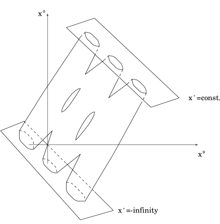
Figure 1: The light-cone setting. We consider the configurations of the Wilson loops which possess the identical light-cone time $x^{+}$. We also locate a group of the Wilson loops at $x^{+}=-\infty$ which represent a particular initial state. We put $k^{+}(\sigma)=1$ for all the Wison loops by using the reparametrization invariance.

In the light-cone setting, the loop equation (9) reduces to

$$k^{(b)-}(\sigma)\langle\tilde{w}(C_{1})\cdots\tilde{w}(C_{b})\cdots\tilde{w}(C_{l})\rangle$$

$$=i\frac{\delta}{\delta x^{(b)+}(\sigma)}\langle\tilde{w}(C_{1})\cdots\tilde{w}(C_{b})\cdots\tilde{w}(C_{l})\rangle$$

$$=\frac{1}{2}(k^{(b)i}(\sigma)^{2}+x^{\prime(b)i}(\sigma)^{2})\langle\tilde{w}(C_{1})\cdots\tilde{w}(C_{b})\cdots\tilde{w}(C_{l})\rangle.$$ (12)

Equation (10) reduces to

$$x^{\prime(b)-}(\sigma)\langle\tilde{w}(C_{1})\cdots\tilde{w}(C_{b})\cdots\tilde{w}(C_{l})\rangle$$

$$=-i\left(\frac{\delta}{\delta k^{(b)+}(\sigma)}\right)^{\prime}\langle\tilde{w}(C_{1})\cdots\tilde{w}(C_{b})\cdots\tilde{w}(C_{l})\rangle$$

$$=x^{\prime(b)i}(\sigma)k_{(b)i}(\sigma)\langle\tilde{w}(C_{1})\cdots\tilde{w}(C_{b})\cdots\tilde{w}(C_{l})\rangle.$$ (13)

Using these equations we can deform the Wilson loop locally from the constant $x^{+}$ surface and shift the value of $k^{(b)+}(\sigma)$ locally. Therefore we can recover general configurations of the Wilson loops. This fact ensures us to consider the light-cone setting. Integrating Eq. (12) over $\sigma$ and summing up over $b$, we obtain an operator which shift the constant value of $x^{+}$, that is, the light-cone Hamiltonian:

$$i\frac{\partial}{\partial x^{+}}\langle\tilde{w}(C_{1})\cdots\tilde{w}(C_{b})\cdots\tilde{w}(C_{l})\rangle$$

$$=\sum_{b}\int d\sigma\frac{1}{2}(k^{(b)i}(\sigma)^{2}+x^{\prime(b)i}(\sigma)^{2})\langle\tilde{w}(C_{1})\cdots\tilde{w}(C_{b})\cdots\tilde{w}(C_{l})\rangle,$$ (14)

which is identical to the free light-cone Hamiltonian of bosonic string. Note that we can obtain a closed system of equations within the light-cone setting even though we consider the particular configurations of the Wilson loops. Our procedure is analogous to obtaining a Hamiltonian in super-many-time theory, where a Hamiltonian density is defined on a general space-like surface. We consider a constant time surface and integrate a Hamiltonian density on it to obtain an ordinary Hamiltonian.

2.2 Loop equations and loop space

In this subsection, we represent our loop equations by the loop space variables and put them in the light-cone setting.

The loop equation (2) is evaluated as

$$0 = \frac{1}{g^{2}}\left\langle({\rm Tr}\left([A_{\nu},[A^{\mu},A^{\nu}]]+\frac{1}{2}\{\bar{\psi}\Gamma^{\mu},\psi\}\right)v(C_{1}))w(C_{2})\cdots w(C_{l})\right\rangle$$ (15)

$$+i\int_{0}^{2\pi}d\sigma k_{\mu}^{(1)}(\sigma)\big{\langle}{\rm Tr}\big{(}Pe^{i\int_{0}^{\sigma}d\sigma^{\prime}(k^{(1)\mu}(\sigma^{\prime})A_{\mu}+\bar{\lambda}^{(1)}(\sigma^{\prime})\psi)}\big{)}$$

$$\times{\rm Tr}\big{(}Pe^{i\int_{\sigma}^{2\pi}d\sigma^{\prime\prime}(k^{(1)\mu}(\sigma^{\prime\prime})A_{\mu}+\bar{\lambda}^{(1)}(\sigma^{\prime\prime})\psi)}\big{)}w(C_{2})\cdots w(C_{l})\big{\rangle}$$

$$+i\sum_{b=2}^{l}\int_{0}^{2\pi}d\sigma k_{\mu}^{(b)}(\sigma)\big{\langle}{\rm Tr}\big{(}Pe^{i\int_{\sigma}^{2\pi}d\sigma^{\prime}(k^{(b)\mu}(\sigma^{\prime})A_{\mu}+\bar{\lambda}^{(b)}(\sigma^{\prime})\psi)}v(C_{1})$$

$$\times Pe^{i\int_{0}^{\sigma}d\sigma^{\prime\prime}(k^{(b)\mu}(\sigma^{\prime\prime})A_{\mu}+\bar{\lambda}^{(b)}(\sigma^{\prime\prime})\psi)}\big{)}w(C_{2})\cdots\check{w}(C_{b})\cdots w(C_{l})\big{\rangle},$$

where $\check{w}(C_{b})$ implies the absence of the Wilson loop $w(C_{b})$. The first term in Eq. (15) represents the infinitesimal deformation of the string coming from the variation of the action $S$ while the second and third terms represent the splitting and joining interaction of strings respectively. Similarly, the loop equation (3) is evaluated as

$$0 = \frac{1}{g^{2}}\langle({\rm Tr}(\Gamma^{\mu}[A_{\mu},\psi]v(C_{1}))w(C_{2})\cdots w(C_{l})\rangle$$ (16)

$$+i\int_{0}^{2\pi}d\sigma\lambda^{(1)}(\sigma)\big{\langle}{\rm Tr}\big{(}Pe^{i\int_{0}^{\sigma}d\sigma^{\prime}(k^{(1)\mu}(\sigma^{\prime})A_{\mu}+\bar{\lambda}^{(1)}(\sigma^{\prime})\psi)}\big{)}$$

$$\times{\rm Tr}\big{(}Pe^{i\int_{\sigma}^{2\pi}d\sigma^{\prime\prime}(k^{(1)\mu}(\sigma^{\prime\prime})A_{\mu}+\bar{\lambda}^{(1)}(\sigma^{\prime\prime})\psi)}\big{)}w(C_{2})\cdots w(C_{l})\big{\rangle}$$

$$+i\sum_{b=2}^{l}\int_{0}^{2\pi}d\sigma\lambda^{(b)}(\sigma)\big{\langle}{\rm Tr}\big{(}Pe^{i\int_{\sigma}^{2\pi}d\sigma^{\prime}(k^{(b)\mu}(\sigma^{\prime})A_{\mu}+\bar{\lambda}^{(b)}(\sigma^{\prime})\psi)}v(C_{1})$$

$$\times Pe^{i\int_{0}^{\sigma}d\sigma^{\prime\prime}(k^{(b)\mu}(\sigma^{\prime\prime})A_{\mu}+\bar{\lambda}^{(b)}(\sigma^{\prime\prime})\psi)}\big{)}w(C_{2})\cdots\check{w}(C_{b})\cdots w(C_{l})\big{\rangle}.$$

We need to represent these equations as differential operators on the loop space. Then we treat field insertions in the loop such as

$${\rm Tr}([A_{\mu},\psi]v(C)).$$ (17)

We have the following identity,

$${\rm Tr}([A_{\mu},\psi]v(C))$$ (18)

$$= -\left(\frac{\delta}{\delta k^{\mu}(\frac{\epsilon}{2})}-\frac{\delta}{\delta k^{\mu}(-\frac{\epsilon}{2})}\right)\frac{\delta}{\delta\bar{\lambda}(0)}w(C)$$

$$-\epsilon\left(\frac{\delta}{\delta k^{\mu}(\frac{\epsilon}{2})}-\frac{\delta}{\delta k^{\mu}(-\frac{\epsilon}{2})}\right)\frac{\delta}{\delta\bar{\lambda}(0)}\left(k^{\nu}(0)\frac{\delta}{\delta k^{\nu}(0)}+\bar{\lambda}(0)\frac{\delta}{\delta\bar{\lambda}(0)}\right)w(C)$$

$$+\mbox{higher order of $\epsilon$}.$$

Though the right-hand side of Eq. (18) vanishes in naive $\epsilon\rightarrow 0$ limit, we expect here that for finite $N$ an ultraviolet cut-off $\epsilon$ appears naturally on the worldsheet. We assume that $\epsilon$ converges to zero in $N\rightarrow\infty$ limit such as $\epsilon\sim N^{-b}\;(b>0)$. We should keep $\epsilon$ and other quantities depending on $N$ in the process of the calculation and take $N\rightarrow\infty\;(\epsilon\rightarrow 0)$ limit as the continuum limit in the final stage.

We expect naively that we may ignore the terms except the first one in the right-hand sides of Eq. (18) since they are the higher order terms with respect to $\epsilon$. However, in general, they contribute to the renormalization of the lower-dimensional terms because in the loop equations they generate the divergences from operator product expansion. The ways we represent the loop equations are not unique since the right-hand sides of Eq. (18) can be expressed in infinitely many ways. However we expect that they are unique in the $\epsilon\rightarrow 0$ limit in the loop equation. This is the universality of the differential operators, which is guaranteed by a power counting and symmetry as seen in §2.4. Here we may draw an analogy with the quantum field theory on the lattice. The lattice action may be expanded formally in terms of the lattice spacing $a$. Although the operators which are suppressed by the powers of $a$ formally vanish in the continuum, we cannot simply neglect them because they may renormalize the relevant operators. In fact we can write down many lattice actions which possess the identical continuum limit.

In the following, we often show only the naive leading terms in the loop equations. Note that we cannot, in fact, neglect infinitely many higher order terms of $\epsilon$ as is discussed above.

By multiplying Eq. (15) by $-ik_{\mu}^{(1)}(0)$, we obtain

$$0 = \frac{1}{g^{2}}\bigg{\langle}\bigg{(}-\frac{1}{\epsilon}\left(\frac{\delta}{\delta k^{(1)\mu}(\frac{\epsilon}{2})}-\frac{\delta}{\delta k^{(1)\mu}(-\frac{\epsilon}{2})}\right)^{2}$$

$$-ik^{(1)}_{\mu}(0)\left(\frac{\delta}{\delta\bar{\lambda}^{(1)}(\frac{\epsilon}{2})}-\frac{\delta}{\delta\bar{\lambda}^{(1)}(-\frac{\epsilon}{2})}\right)\Gamma^{0}\Gamma^{\mu}\frac{\delta}{\delta\bar{\lambda}^{(1)}(-\frac{\epsilon}{2})}\bigg{)}w(C_{1})\cdots w(C_{l})\bigg{\rangle}$$

$$+\int_{0}^{2\pi}d\sigma k^{(1)\mu}(0)k_{\mu}^{(1)}(\sigma)\big{\langle}{\rm Tr}\big{(}Pe^{i\int_{0}^{\sigma}d\sigma^{\prime}(k^{(1)\mu}(\sigma^{\prime})A_{\mu}+\bar{\lambda}^{(1)}(\sigma^{\prime})\psi)}\big{)}$$

$$\times{\rm Tr}\big{(}Pe^{i\int_{\sigma}^{2\pi}d\sigma^{\prime\prime}(k^{(1)\mu}(\sigma^{\prime\prime})A_{\mu}+\bar{\lambda}^{(1)}(\sigma^{\prime\prime})\psi)}\big{)}w(C_{2})\cdots w(C_{l})\big{\rangle}$$

$$+\sum_{b=2}^{l}\int_{0}^{2\pi}d\sigma k^{(1)\mu}(0)k_{\mu}^{(b)}(\sigma)\big{\langle}{\rm Tr}\big{(}Pe^{i\int_{0}^{\sigma}d\sigma^{\prime}(k^{(b)\mu}(\sigma^{\prime})A_{\mu}+\bar{\lambda}^{(b)}(\sigma^{\prime})\psi)}$$

$$\times v(C_{1})Pe^{i\int_{\sigma}^{2\pi}d\sigma^{\prime\prime}(k^{(b)\mu}(\sigma^{\prime\prime})A_{\mu}+\bar{\lambda}^{(b)}(\sigma^{\prime\prime})\psi)}\big{)}w(C_{2})\cdots\check{w}(C_{b})\cdots w(C_{l})\big{\rangle}.$$

Similarly, Eq. (16) is represented as

$$0 = \frac{i}{g^{2}}\left\langle\left(\frac{\delta}{\delta k^{(1)\mu}(\frac{\epsilon}{2})}-\frac{\delta}{\delta k^{(1)\mu}(-\frac{\epsilon}{2})}\right)\Gamma^{\mu}\frac{\delta}{\delta\bar{\lambda}^{(1)}(0)}w(C_{1})\cdots w(C_{l})\right\rangle$$

$$+\int_{0}^{2\pi}d\sigma\lambda^{(1)}(\sigma)\big{\langle}{\rm Tr}\big{(}Pe^{i\int_{0}^{\sigma}d\sigma^{\prime}(k^{(1)\mu}(\sigma^{\prime})A_{\mu}+\bar{\lambda}^{(1)}(\sigma^{\prime})\psi)}\big{)}$$

$$\times{\rm Tr}\big{(}Pe^{i\int_{\sigma}^{2\pi}d\sigma^{\prime\prime}(k^{(1)\mu}(\sigma^{\prime\prime})A_{\mu}+\bar{\lambda}^{(1)}(\sigma^{\prime\prime})\psi)}\big{)}w(C_{2})\cdots w(C_{l})\big{\rangle}$$

$$+\sum_{b=2}^{l}\int_{0}^{2\pi}d\sigma\lambda^{(b)}(\sigma)\big{\langle}{\rm Tr}\big{(}Pe^{i\int_{\sigma}^{2\pi}d\sigma^{\prime}(k^{(b)\mu}(\sigma^{\prime})A_{\mu}+\bar{\lambda}^{(b)}(\sigma^{\prime})\psi)}$$

$$\times v(C_{1})Pe^{i\int_{0}^{\sigma}d\sigma^{\prime\prime}(k^{(b)\mu}(\sigma^{\prime\prime})A_{\mu}+\bar{\lambda}^{(b)}(\sigma^{\prime\prime})\psi)}\big{)}w(C_{2})\cdots\check{w}(C_{b})\cdots w(C_{l})\big{\rangle}.$$

Here let us proceed to the light-cone setting. The $+$ component of total momentum carried by the $\tilde{w}[x^{+}(\sigma^{\prime})=x^{+},k^{+}(\sigma^{\prime})=1,k^{i}(\sigma^{\prime}),\lambda(\sigma^{\prime});\sigma^{\prime}=0\sim\sigma)]$ is equal to $\sigma$. Therefore we expect naively

$$\langle\tilde{w}[x^{+}(\sigma^{\prime})=x^{+},k^{+}(\sigma^{\prime})=1,k^{i}(\sigma^{\prime}),\lambda(\sigma);\sigma^{\prime}=0\sim\sigma)]\rangle=0$$ (21)

because of the momentum conservation if $\sigma\neq 0$. We also expect the same case for $\langle\tilde{w}[x^{+}(\sigma^{\prime})=x^{+},k^{+}(\sigma^{\prime})=1,k^{i}(\sigma^{\prime}),\lambda(\sigma^{\prime});\sigma^{\prime}=p^{+}-\sigma\sim p^{+}]\rangle$. However these are not actually the cases since the eigenvalues of $A_{\mu}$ distribute in a finite range for finite $N$, which violates the momentum conservation slightly. Therefore these two $\tilde{w}$ have support for small $\sigma$ generally. We define a nonvanishing quantity $I$ by

$$I = \int_{0}^{p^{+}}d\sigma\langle\tilde{w}[x^{+}(\sigma^{\prime})=x^{+},k^{+}(\sigma^{\prime})=1,k^{i}(\sigma^{\prime}),\lambda(\sigma);\sigma^{\prime}=0\sim\sigma]$$ (22)

$$+\tilde{w}[x^{+}(\sigma^{\prime})=x^{+},k^{+}(\sigma^{\prime})=1,k^{i}(\sigma^{\prime}),\lambda(\sigma);\sigma^{\prime}=p^{+}-\sigma\sim p^{+}]\rangle.$$

We expect that $I$ diverges as $N\rightarrow\infty$ and assume that its large $N$ behavior is $I\sim N^{a}\;(a>0)$. Then a part of the splitting interaction term in the loop equations contribute to the first term in the loop equations representing the infinitesimal deformation of the string.

Thus in the light-cone setting Eq. (LABEL:eqA3) leads to

$$k^{(1)-}(0)\langle\tilde{w}(C_{1})\cdots\tilde{w}(C_{l})\rangle$$

$$= \frac{1}{Z}\bigg{\{}\bigg{(}k^{(1)i}(0)^{2}+\frac{\epsilon}{g^{2}I}x^{{}^{\prime}(1)}(0)^{2}$$

$$-i\sqrt{2}\frac{\epsilon}{g^{2}I}\theta^{{}^{\prime}(1)}_{a}(0)\theta^{(1)}_{a}(0)-i\frac{\epsilon}{g^{2}I}k^{(1)i}(0)\gamma^{i}_{a\dot{a}}(\theta^{{}^{\prime}(1)}_{a}(0)\theta^{(1)}_{\dot{a}}(0)+\theta^{{}^{\prime}(1)}_{\dot{a}}(0)\theta^{(1)}_{a}(0))\bigg{)}$$

$$\hskip 142.26378pt\times\langle\tilde{w}(C_{1})\cdots\tilde{w}(C_{l})\rangle$$

$$+\frac{1}{I}\int_{0}^{p^{(1)+}}d\sigma k^{(1)}_{\mu}(0)k^{(1)\mu}(\sigma)\big{\langle}\tilde{\rm Tr}\big{(}Pe^{i\int_{0}^{\sigma}d\sigma^{\prime}(k^{(1)\mu}(\sigma^{\prime})A_{\mu}+\bar{\lambda}^{(1)}(\sigma^{\prime})\psi)}\big{)}$$

$$\times\tilde{\rm Tr}\big{(}Pe^{i\int_{\sigma}^{p^{(1)+}}d\sigma^{\prime\prime}(k^{(1)\mu}(\sigma^{\prime\prime})A_{\mu}+\bar{\lambda}^{(1)}(\sigma^{\prime\prime})\psi)}\big{)}\tilde{w}(C_{2})\cdots\tilde{w}(C_{l})\big{\rangle}$$

$$+\frac{1}{I}\sum_{b=2}^{l}\int_{0}^{p^{(b)+}}d\sigma k^{(1)}_{\mu}(0)k^{(b)\mu}(\sigma)\big{\langle}\tilde{\rm Tr}\big{(}Pe^{i\int_{\sigma}^{p^{(b)+}}d\sigma^{\prime}(k^{(b)\mu}(\sigma^{\prime})A_{\mu}+\bar{\lambda}^{(b)}(\sigma^{\prime})\psi)}$$

$$\times v(C_{1})Pe^{i\int_{0}^{\sigma}d\sigma^{\prime\prime}(k^{(b)\mu}(\sigma^{\prime\prime})A_{\mu}+\bar{\lambda}^{(b)}(\sigma^{\prime\prime})\psi)}\big{)}\tilde{w}(C_{2})\cdots\check{\tilde{w}}(C_{b})\cdots\tilde{w}(C_{l})\big{\rangle}\bigg{\}}.$$

where $Z$ is defined by

$$Z=2\left(1+\frac{i\epsilon}{\sqrt{2}g^{2}I}\theta^{\prime}_{\dot{a}}(0)\theta_{\dot{a}}(0)\right)$$ (24)

and $\tilde{\rm Tr}$ means that the corresponding Wilson loop is arranged in the light-cone setting. Here $x_{\mu}$, $\theta_{a}$ and $\theta_{\dot{a}}$ are defined as follows:

$$x_{\mu}(\sigma)=i\frac{\delta}{\delta k^{\mu}(\sigma)},$$

$$\theta_{a}(\sigma)=\frac{\delta}{\delta\lambda_{a}(\sigma)},$$

$$\theta_{\dot{a}}(\sigma)=\frac{\delta}{\delta\lambda_{\dot{a}}(\sigma)}.$$ (25)

Equation (LABEL:eqpsi3) is decomposed into two equations as follows.

$$\lambda^{(1)}_{\dot{a}}(0)\langle\tilde{w}(C_{1})\cdots\tilde{w}(C_{l})\rangle$$ (26)

$$= \frac{\epsilon}{g^{2}I}(\sqrt{2}x^{{}^{\prime}(1)-}(0)\theta_{\dot{a}}(0)+x^{{}^{\prime}i(1)}(0)\gamma^{i}_{\dot{a}a}\theta^{(1)}_{a}(0))\langle\tilde{w}(C_{1})\cdots\tilde{w}(C_{l})\rangle$$

$$-\frac{1}{I}\int_{0}^{p^{(1)+}}d\sigma\lambda^{(1)}_{\dot{a}}(\sigma)\big{\langle}\tilde{\rm Tr}\big{(}Pe^{i\int_{0}^{\sigma}d\sigma^{\prime}(k^{(1)\mu}(\sigma^{\prime})A_{\mu}+\bar{\lambda}^{(1)}(\sigma^{\prime})\psi)}\big{)}$$

$$\times\tilde{\rm Tr}\big{(}Pe^{i\int_{\sigma}^{p^{(1)+}}d\sigma^{\prime\prime}(k^{(1)\mu}(\sigma^{\prime\prime})A_{\mu}+\bar{\lambda}^{(1)}(\sigma^{\prime\prime})\psi)}\big{)}\tilde{w}(C_{2})\cdots\tilde{w}(C_{l})\big{\rangle}$$

$$-\frac{1}{I}\sum_{b=2}^{l}\int_{0}^{p^{(b)+}}d\sigma\lambda^{(b)}_{\dot{a}}(\sigma)\big{\langle}\tilde{\rm Tr}\big{(}Pe^{i\int_{\sigma}^{p^{(b)+}}d\sigma^{\prime}(k^{(b)\mu}(\sigma^{\prime})A_{\mu}+\bar{\lambda}^{(b)}(\sigma^{\prime})\psi)}v(C_{1})$$

$$\times Pe^{i\int_{0}^{\sigma}d\sigma^{\prime\prime}(k^{(b)\mu}(\sigma^{\prime\prime})A_{\mu}+\bar{\lambda}^{(b)}(\sigma^{\prime\prime})\psi)}\big{)}\tilde{w}(C_{2})\cdots\check{\tilde{w}}(C_{b})\cdots\tilde{w}(C_{l})\big{\rangle},$$

$$\theta^{(1)}_{\dot{a}}(0)\langle\tilde{w}(C_{1})\cdots\tilde{w}(C_{l})\rangle$$ (27)

$$= \frac{g^{2}I}{\epsilon}(x^{{}^{\prime}(1)i}(0)\gamma^{i}_{a\dot{a}})^{-1}\bigg{\{}\lambda^{(1)}_{a}(0)\langle\tilde{w}(C_{1})\cdots\tilde{w}(C_{l})\rangle$$

$$+\frac{1}{I}\int_{0}^{p^{(1)+}}d\sigma\lambda^{(1)}_{a}(\sigma)\big{\langle}\tilde{\rm Tr}\big{(}Pe^{i\int_{0}^{\sigma}d\sigma^{\prime}(k^{(1)\mu}(\sigma^{\prime})A_{\mu}+\bar{\lambda}^{(1)}(\sigma^{\prime})\psi)}\big{)}$$

$$\times\tilde{\rm Tr}\big{(}Pe^{i\int_{\sigma}^{p^{(1)+}}d\sigma^{\prime\prime}(k^{(1)\mu}(\sigma^{\prime\prime})A_{\mu}+\bar{\lambda}^{(1)}(\sigma^{\prime\prime})\psi)}\big{)}\tilde{w}(C_{2})\cdots\tilde{w}(C_{l})\big{\rangle}$$

$$+\frac{1}{I}\sum_{b=2}^{l}\int_{0}^{p^{(b)+}}d\sigma\lambda^{(b)}_{a}(\sigma)\big{\langle}\tilde{\rm Tr}\big{(}Pe^{i\int_{\sigma}^{p^{(b)+}}d\sigma^{\prime}(k^{(b)\mu}(\sigma^{\prime})A_{\mu}+\bar{\lambda}^{(b)}(\sigma^{\prime})\psi)}v(C_{1})$$

$$\times Pe^{i\int_{0}^{\sigma}d\sigma^{\prime\prime}(k^{(b)\mu}(\sigma^{\prime\prime})A_{\mu}+\bar{\lambda}^{(b)}(\sigma^{\prime\prime})\psi)}\big{)}\tilde{w}(C_{2})\cdots\check{\tilde{w}}(C_{b})\cdots\tilde{w}(C_{l})\big{\rangle}\bigg{\}}.$$

We eliminate a half of fermionic degrees of freedom by using the above two equations just like eliminating the half of the fermionic degrees of freedom in the light-cone field theory by using the equation of motion. We can also rewrite Eq. (4) as

$$x^{{}^{\prime}(1)-}(\sigma)\langle\tilde{w}(C_{1})\cdots\tilde{w}(C_{l})\rangle$$

$$=(k^{(1)i}(\sigma)x^{{}^{\prime}(1)i}(\sigma)+i\lambda^{(1)}_{a}(\sigma)\theta^{(1)}_{a}(\sigma)+i\lambda^{(1)}_{\dot{a}}(\sigma)\theta^{(1)}_{\dot{a}}(\sigma))\langle\tilde{w}(C_{1})\cdots\tilde{w}(C_{l})\rangle.$$

(28)

Our task is summarized as follows. By using Eqs. (LABEL:eqk-), (26), (27) and (28) iteratively and repeatedly, we eliminate $\lambda_{n\dot{a}}$, $\theta_{n\dot{a}}$ and $x^{{}^{\prime}-}$, and evaluate the light-cone Hamiltonian,

$$H=\sum_{b}\int d\sigma k^{(b)-}(\sigma).$$ (29)

In this process, various interaction terms of order $1/I^{k}\sim O(1/N^{ka})$ are generated, which represent processes where the $k+2$ strings interact at one point, i.e., $(k+2)$-Reggeon vertices. In this procedure, we should take the continuum limit by keeping the higher order terms of $\epsilon$ vanishing in the naive $\epsilon\rightarrow 0$ limit. This task is in general very hard to perform because we should treat infinite series. However we will discuss in §2.4 that the continuum limit is completely controllable by an analysis based on a power counting of $\epsilon$ and the symmetries. We should consider the supercharges first rather than the Hamiltonian in this more rigorous treatment. In the next subsection, we first sketch how we can derive light-cone Hamiltonian for type IIB superstring from the loop equations.

2.3 Light-cone Hamiltonian

Here we neglect the interaction terms in Eq. (LABEL:eqk-) and concentrate on the free part of light-cone Hamiltonian. We can see that if we ignore the non-quadratic terms and set $\frac{g^{2}I}{\epsilon}\sim\alpha^{{}^{\prime}2}\sim$ const, the free part of Eq. (LABEL:eqk-) has the same form as the free light-cone Hamiltonian of type IIB superstring in the naive continuum limit except lacking the $\lambda^{\prime}_{a}\lambda_{a}$ term. In the following, we verify that we indeed obtain this term when we eliminate $\theta_{\dot{a}}$ in the free part of Eq. (LABEL:eqk-) using Eq. (27). Let us consider the naive leading contribution in the free part of Eq. (27):

$$\theta^{(1)}_{\dot{a}}(\sigma)\langle w(C_{1})\cdots w(C_{l})\rangle={x^{{}^{\prime}(1)}_{i}(\sigma)\gamma^{i}_{\dot{a}a}\over x^{{}^{\prime}(1)}_{i}(\sigma)^{2}}{g^{2}I\over\epsilon}\lambda^{(1)}_{a}(\sigma)\langle w(C^{1})w(C^{2})\cdots w(C^{l})\rangle.$$ (30)

We assume first that the free part of Eq. (LABEL:eqk-) correctly describes the free part of light-cone Hamiltonian. This assumption can be justified by showing that the non-quadratic terms are indeed negligible in the continuum limit except for finite renormalization of the quadratic terms. Since we are dealing with free two-dimensional field theories, we can use standard techniques of conformal field theory to estimate the effects of the non-quadratic terms. We note that the $x^{{}^{\prime}(1)}_{i}(\sigma)^{2}$ is of order $1/\epsilon^{2}$ since we have a cutoff length $\epsilon$. So we may expand $x^{{}^{\prime}(1)}_{i}(\sigma)^{2}=1/\alpha\epsilon^{2}+:x^{{}^{\prime}(1)}_{i}(\sigma)^{2}:$, where $:y:$ denotes the normal ordered operator constructed out of $y$. The symbol $\alpha$ in the denominator is a quantity proportional to $\sqrt{\epsilon/g^{2}I}$ on dimensional grounds. In this way, the left-hand side of Eq. (30) becomes

$$\epsilon^{2}{\alpha g^{2}I\over{\epsilon}}x^{{}^{\prime}(1)}_{i}(\sigma)\gamma^{i}_{\dot{a}a}(1-\epsilon^{2}\alpha:x^{{}^{\prime}(1)}_{i}(\sigma)^{2}:+\cdots)\lambda^{(1)}_{a}(\sigma)\langle w(C_{1})\cdots w(C_{l})\rangle.$$ (31)

For example, a typical non-quadratic term in the free part of Eq. (LABEL:eqk-),

$$\epsilon^{4}k^{(1)i}(\sigma)^{2}x^{{}^{\prime}(1)j}(\sigma)\gamma^{j}_{\dot{a}a}\lambda^{{}^{\prime}(1)}_{a}(\sigma)x^{{}^{\prime}(1)k}(\sigma)\gamma^{k}_{\dot{a}b}\lambda^{{}^{\prime}(1)}_{b}(\sigma),$$ (32)

generates the $\lambda^{{}^{\prime}(1)}_{a}(\sigma)\lambda^{(1)}_{a}(\sigma)$ term due to the order $1/\epsilon^{4}$ divergence from the operator product expansion of $k^{(1)i}(\sigma)^{2}x^{{}^{\prime}j(1)}(\sigma)x^{{}^{\prime}(1)k}(\sigma)$.

In this way, we see that non-quadratic higher-dimensional operators do not appear in the continuum limit due to the suppression of the powers of $\epsilon$ and only renormalize finitely the quadratic operators. Therefore we expect to obtain the following free Hamiltonian in the continuum limit:

$$H_{\rm free} = \sum_{b}\int_{0}^{p^{(b)+}}d\sigma{1\over 2}\bigg{(}ck^{(b)i}(\sigma)^{2}+c^{\prime}\frac{\epsilon}{g^{2}I}x^{{}^{\prime}(1)i}(\sigma)^{2}-ic^{\prime\prime}\lambda^{{}^{\prime}(b)}_{a}(\sigma)\lambda^{(b)}_{a}(\sigma)$$ (33)

$$\hskip 85.35826pt-ic^{\prime\prime\prime}\frac{1}{g^{2}N}\theta^{{}^{\prime}(b)}_{a}(\sigma)\theta^{(b)}_{a}(\sigma)\bigg{)}.$$

Here we assume that terms with the negative powers of $\epsilon$ and other finite terms such as $k^{i}x^{\prime i}$ do not remain, which is guaranteed by an argument based on a power counting and symmetries as is seen in the next subsection. In the bosonic model, this is not guaranteed and the $1/\epsilon^{2}$ divergence remains in general. This is the reason why we cannot obtain the light-cone string field theory from the bosonic reduced model. The Hamiltonian (33) is identical to that of type IIB superstring theory[18] if $\lambda_{a}(\sigma)$ and $\theta_{a}(\sigma)$ are rescaled appropriately and rotated by a complex phase factor $\eta=\exp({i\pi\over 4})$ as follows:

$$\lambda_{a}(\sigma)\rightarrow\eta\lambda_{a}(\sigma),~{}\theta_{a}(\sigma)\rightarrow\eta^{*}\theta_{a}(\sigma).$$ (34)

We elaborate more on this point in connection with the supercharges in the next subsection. Here we cannot determine the coefficients $c$, $c^{\prime}$, $c^{\prime\prime}$ and $c^{\prime\prime\prime}$, which include the effects of renormalizations, and in the next subsection we can fix them by using $\mathcal{N}$=2 supersymmetry. From Eq. (33) we find $\alpha^{\prime 2}\sim g^{2}I/\epsilon$ and hence we should obtain the prescription of the scaling limit, $g^{2}N^{a+b}\sim\alpha^{\prime 2}\sim$ const.

2.4 General proof

In this subsection, we give a general proof of our assertion that the light-cone string field theory for type IIB superstring can be derived from the loop equations of the IIB matrix model. We use a power counting and a symmetry analysis based on $\mathcal{N}$=2 supersymmetry, $SO(8)$ invariance and the parity symmetry on the string worldsheet.

2.4.1 Power counting and parity symmetry

In order to perform a power counting for $\epsilon$, we first introduce a mass dimension on the worldsheet through the relation $[\epsilon]=-1$ and determine the dimension of each field. The IIB matrix model action (1) is decomposed into

$$S = -{1\over g^{2}}{\rm Tr}\bigg{(}-\frac{1}{2}[A^{+},A^{-}]^{2}-[A^{+},A^{i}][A^{-},A^{i}]+{1\over 4}[A^{i},A^{j}]^{2}$$

$$+{1\over 2}(\sqrt{2}\psi_{{a}}[A^{+},\psi_{{a}}]-\psi_{a}\gamma^{i}_{{a}\dot{a}}[A^{i},\psi_{\dot{a}}]-\psi_{\dot{a}}\gamma^{i}_{\dot{a}{a}}[A^{i},\psi_{{a}}]+\sqrt{2}\psi_{\dot{a}}[A^{-},\psi_{\dot{a}}])\bigg{)}.$$

By demanding the IIB matrix model action (LABEL:SO(8)decomposition) to be dimensionless, we obtain

$$[A^{i}]=0,\>[A^{+}]=-[A^{-}],\>[A^{+}]=-2[\psi_{a}]\quad\mbox{and}\quad[A^{-}]=-2[\psi_{\dot{a}}].$$ (36)

On the other hand, the Wilson loop (1) is decomposed into

$$w(C) = {\rm Tr}\big{(}P\exp\big{(}i\int_{0}^{p^{+}}d\sigma(-k^{+}(\sigma)A^{-}$$ (37)

$$-k^{-}(\sigma)A^{+}+k^{i}(\sigma)A^{i}-i\lambda_{a}(\sigma)\psi_{a}-i\lambda_{\dot{a}}(\sigma)\psi_{\dot{a}}\big{)}\big{)}.$$

From this, we also read off the relations

$$[k^{+}]+[A^{-}]=1,$$

$$[k^{-}]+[A^{+}]=1,$$

$$[k^{i}]+[A^{i}]=1,$$

$$[\lambda_{a}]+[\psi_{a}]=1,$$

$$[\lambda_{\dot{a}}]+[\psi_{\dot{a}}]=1.$$ (38)

Noting that we should set $[k^{+}]$ to be zero since $k^{+}(\sigma)=1$ in our light-cone setting, we can determine the dimensions of all quantities as follows:

$$[k^{+}]=0,\>[k^{-}]=2,\>[k^{i}]=1,\>[\lambda_{a}]=\frac{1}{2},\>[\lambda_{\dot{a}}]=\frac{3}{2},$$

$$[x^{+}]=-1,\>[x^{-}]=1,\>[x^{i}]=0,\>[\theta_{a}]=\frac{1}{2},\>[\theta_{\dot{a}}]=-\frac{1}{2},$$

$$[A^{+}]=-1,\>[A^{-}]=1,\>[A^{i}]=0,\>[\psi_{a}]=\frac{1}{2},\>[\psi_{\dot{a}}]=-\frac{1}{2}.$$ (39)

Next we define a symmetry which corresponds to the parity on the string worldsheet. It is seen easily that the IIB matrix model action (1) is formally invariant under the following transformation:

$$A_{\mu}\rightarrow A_{\mu}^{t},$$

$$\psi\rightarrow-i\psi^{t}.$$ (40)

This transformation flips the direction of the Wilson loop in the following way:

$$w(C) = {\rm Tr}\left(Pe^{i\int_{0}^{p^{+}}d\sigma(k^{\mu}(\sigma)A_{\mu}+\bar{\lambda}(\sigma)\psi)}\right)$$ (41)

$$\hskip 56.9055pt\rightarrow{\rm Tr}\left(P\prod^{M}_{n=1}e^{i\int_{0}^{p^{+}}d\sigma(k^{\mu}(p^{+}-\sigma)A_{\mu}-i\bar{\lambda}(p^{+}-\sigma)\psi)}\right).$$

Therefore our theory has a symmetry under the transformation

$$k^{\mu}(\sigma)\rightarrow k^{\mu}(p^{+}-\sigma),$$

$$\lambda(\sigma)\rightarrow i\lambda(p^{+}-\sigma),$$ (42)

which we identify with the worldsheet parity. We also obtain the parity transformation for the dual variables $x^{\mu}_{n}$ and $\theta_{n}$:

$$x^{\mu}(\sigma)\rightarrow x^{\mu}(p^{+}-\sigma),$$

$$\theta(\sigma)\rightarrow-i\theta(p^{+}-\sigma).$$ (43)

2.4.2 $\mathcal{N}$=2 supersymmetry

We denote the supercharges generating the transformations

$$\cases{\delta^{(1)}A_{\mu}&$=i\bar{\varepsilon}\Gamma_{\mu}\psi$\cr\delta^{(1)}\psi&$=\frac{i}{2}\Gamma^{\mu\nu}[A^{\mu},A^{\nu}]{\varepsilon}$}$$ (44)

and

$$\cases{\delta^{(2)}A_{\mu}&= 0\cr\delta^{(2)}\psi&$=\xi$,}$$ (45)

by $Q^{(1)}$ and $Q^{(2)}$ respectively. We can determine the dimensions and parities of the parameters $\varepsilon$ and $\xi$ in Eqs. (44) and (45) by comparing their both sides,

$$[\varepsilon_{a}]=[\xi_{a}]=\frac{1}{2},\>[\varepsilon_{\dot{a}}]=[\xi_{\dot{a}}]=-\frac{1}{2},$$

$$\varepsilon_{a}\rightarrow i\varepsilon_{a},\>\varepsilon_{\dot{a}}\rightarrow i\varepsilon_{\dot{a}},$$

$$\xi_{a}\rightarrow-i\xi_{a},\>\xi_{\dot{a}}\rightarrow-i\xi_{\dot{a}}.$$ (46)

This fixes the dimensions and parities of the supercharges $Q^{(1)}$ and $Q^{(2)}$ since $\varepsilon_{a}Q^{(1)}_{a}+\varepsilon_{\dot{a}}Q^{(1)}_{\dot{a}}+\xi_{a}Q^{(2)}_{a}+\xi_{\dot{a}}Q^{(2)}_{\dot{a}}$ generates the transformations (44) and (45):

$$[Q^{(1)}_{a}]=[Q^{(2)}_{a}]=-\frac{1}{2},\>[Q^{(1)}_{\dot{a}}]=[Q^{(2)}_{\dot{a}}]=\frac{1}{2},$$ (47)

$$Q^{(1)}_{a}\rightarrow-iQ^{(1)}_{a},\>Q^{(1)}_{\dot{a}}\rightarrow-iQ^{(1)}_{\dot{a}},$$

$$Q^{(2)}_{a}\rightarrow iQ^{(2)}_{a},\>Q^{(2)}_{\dot{a}}\rightarrow iQ^{(2)}_{\dot{a}}.$$ (48)

Here we note that Eqs. (47) and (48) are consistent with the anti-commutation relations

$$\{Q^{(1)},Q^{(1)}\}=0,\>\{Q^{(2)},Q^{(2)}\}=0,$$

$$\{Q^{(1)}_{a},Q^{(2)}_{b}\}=\sqrt{2}P^{+}\delta_{ab},$$

$$\{Q^{(1)}_{a},Q^{(2)}_{\dot{a}}\}=P^{i}\gamma^{i}_{a\dot{a}},\>\{Q^{(1)}_{\dot{a}},Q^{(2)}_{a}\}=P^{i}\gamma^{i}_{\dot{a}a},$$

$$\{Q^{(1)}_{\dot{a}},Q^{(2)}_{\dot{b}}\}=\sqrt{2}H\delta_{\dot{a}\dot{b}}.$$ (49)

2.4.3 Free parts of supercharges and Hamiltonian

The supercharges $Q^{(1)}$ and $Q^{(2)}$ can be expressed as differential operators on the loop space using the Ward identities. In principle we can eliminate the operators $k^{-}$, $x^{{}^{\prime}-}$, $\lambda_{\dot{a}}$ and $\theta_{\dot{a}}$ by repeatedly using the loop equations and the reparametrization invariance as is discussed for $k^{-}$ in the previous section. Note that we obtain interaction terms through this procedure. However as we will see just below, the forms of their continuum limit are completely determined by the dimension, parity and $SO(8)$ invariance. First we concentrate on free parts of the supercharges $Q^{(1)}$ and $Q^{(2)}$, i.e., ignore the interaction terms. By using the power counting, Eqs. (39) and (47), $SO(8)$ invariance and the parity symmetry, Eqs. (42), (43) and (48), we can deduce the following forms of free supercharges in the $\epsilon\rightarrow 0$ limit:

$$Q^{(1)}_{{\rm free}\,a}=\int d\sigma a_{1}\theta_{a}(\sigma),$$

$$Q^{(2)}_{{\rm free}\,a}=\int d\sigma a_{2}\lambda_{a}(\sigma),$$

$$Q^{(1)}_{{\rm free}\,\dot{a}}=\int d\sigma(b_{1}x^{\prime i}(\sigma)\gamma^{i}_{\dot{a}a}\lambda_{a}(\sigma)+c_{1}k^{i}(\sigma)\gamma^{i}_{\dot{a}a}\theta_{a}(\sigma)),$$

$$Q^{(2)}_{{\rm free}\,\dot{a}}=\int d\sigma(b_{2}k^{i}(\sigma)\gamma^{i}_{\dot{a}a}\lambda_{a}(\sigma)+c_{2}x^{\prime i}(\sigma)\gamma^{i}_{\dot{a}a}\theta_{a}(\sigma)).$$ (50)

In Eq. (50) we have excluded terms such as $\frac{1}{\epsilon}x^{i}\gamma^{i}\lambda$ by translation invariance. It is easy to see that all possible terms which appear with negative powers of $\epsilon$ are forbidden by the symmetries. In this sense the existence of the continuum limit is guaranteed by the symmetries. We can also fix undetermined coefficients in Eq. (50) by the $\mathcal{N}$=2 supersymmetry (49) as follows. From $\{Q^{(1)}_{a},Q^{(2)}_{b}\}=\sqrt{2}P^{+}\delta_{ab}$, $\{Q^{(1)}_{a},Q^{(2)}_{\dot{a}}\}=P^{i}\gamma^{i}_{a\dot{a}}$ and $\{Q^{(1)}_{\dot{a}},Q^{(2)}_{a}\}=P^{i}\gamma^{i}_{\dot{a}a}$, we obtain

$$a_{1}a_{2}=\sqrt{2},\>a_{1}b_{2}=1\quad\mbox{and}\quad a_{2}c_{1}=1.$$ (51)

Therefore Eq. (50) is reduced to

$$Q^{(1)}_{{\rm free}\,a}=a_{1}\int d\sigma\theta_{a}(\sigma),$$

$$Q^{(2)}_{{\rm free}\,a}=\frac{\sqrt{2}}{a_{1}}\int d\sigma\lambda_{a}(\sigma),$$

$$Q^{(1)}_{{\rm free}\,\dot{a}}=\int d\sigma\left(\frac{a_{1}}{\sqrt{2}}k^{i}(\sigma)\gamma^{i}_{\dot{a}a}\theta_{a}(\sigma)+b_{1}x^{\prime i}(\sigma)\gamma^{i}_{\dot{a}a}\lambda_{a}(\sigma)\right),$$

$$Q^{(2)}_{{\rm free}\,\dot{a}}=\int d\sigma\left(\frac{1}{a_{1}}k^{i}(\sigma)\gamma^{i}_{\dot{a}a}\lambda_{a}(\sigma)+c_{2}x^{\prime i}(\sigma)\gamma^{i}_{\dot{a}a}\theta_{a}(\sigma)\right).$$ (52)

The free part of the Hamiltonian $\int d\sigma k^{-}(\sigma)$ is obtained by $\{Q^{(1)}_{\dot{a}},Q^{(2)}_{\dot{b}}\}=\sqrt{2}H\delta_{\dot{a}\dot{b}}$ as

$$H_{\rm free}=\int d\sigma\left(\frac{1}{2}k^{i}(\sigma)^{2}+\frac{1}{\sqrt{2}}b_{1}c_{2}x^{\prime i}(\sigma)^{2}-i\frac{b_{1}}{\sqrt{2}a_{1}}\lambda^{\prime}_{a}(\sigma)\lambda_{a}(\sigma)-i\frac{a_{1}c_{2}}{2}c_{2}\theta^{\prime}_{a}(\sigma)\theta_{a}(\sigma)\right).\\$$

In order to compare these results with the Green-Schwarz light-cone formalism, we redefine the fermionic variables as

$$\lambda_{a}=\sqrt{\frac{a_{1}}{b_{1}}}\eta\check{\lambda}_{a}\quad\mbox{and}\quad\theta_{a}=\sqrt{\frac{b_{1}}{a_{1}}}\eta^{*}\check{\theta}_{a},$$ (53)

where $\eta=e^{\frac{\pi i}{4}}$. We also introduce rescaled supercharges $\check{Q}^{1}$ and $\check{Q}^{2}$ by

$$Q^{(1)}=\sqrt{a_{1}b_{1}}\eta^{*}\check{Q}^{1}\quad\mbox{and}\quad Q^{(2)}=\frac{\eta}{\sqrt{a_{1}b_{1}}}\check{Q}^{(2)}.$$ (54)

In terms of these new quantities, Eqs. (52) and (2.4.3) become

$$\check{Q}^{1}_{{\rm free}\,a}=\int d\sigma\check{\theta}_{a}(\sigma),$$

$$\check{Q}^{(2)}_{{\rm free}\,a}=\sqrt{2}\int d\sigma\check{\lambda}_{a}(\sigma),$$

$$\check{Q}^{1}_{{\rm free}\,\dot{a}}=\int d\sigma\left(\frac{1}{\sqrt{2}}k^{i}(\sigma)\gamma^{i}_{\dot{a}a}\check{\theta}_{a}(\sigma)+ix^{\prime i}(\sigma)\gamma^{i}_{\dot{a}a}\check{\lambda}_{a}(\sigma)\right),$$

$$\check{Q}^{(2)}_{{\rm free}\,\dot{a}}=\int d\sigma(k^{i}(\sigma)\gamma^{i}_{\dot{a}a}\check{\lambda}_{a}(\sigma)-ib_{1}c_{2}x^{\prime i}(\sigma)\gamma^{i}_{\dot{a}a}\check{\theta}_{a}(\sigma)),$$

$$H_{\rm free}=\int d\sigma\left(\frac{1}{2}k^{i}(\sigma)^{2}+\frac{1}{\sqrt{2}}b_{1}c_{2}x^{\prime i}(\sigma)^{2}+\frac{1}{\sqrt{2}}\check{\lambda}^{\prime}_{a}(\sigma)\check{\lambda}_{a}(\sigma)-\frac{1}{2}b_{1}c_{2}\check{\theta}^{\prime}_{a}(\sigma)\check{\theta}_{a}(\sigma)\right),$$

which completely agree with the light-cone Green-Schwarz free Hamiltonian and supercharges for type IIB superstring. This fact also justifies the analytic continuation introduced for fermionic fields in Ref. IKKT. We also note that we have obtained the relation $b_{1}c_{2}\sim 1/\alpha^{\prime 2}$, and $b_{1}c_{2}$ should be equal to $\epsilon/g^{2}I$ multiplied by some numerical constant as is illustrated in the previous subsection.

2.4.4 Interaction parts of supercharges and Hamiltonian

In this subsection, we examine the structure of the interaction parts of the supercharges and the Hamiltonian. First we consider the contributions of order $1/I$, which correspond to 3-Reggeon vertices in string field theory. Since our free Hamiltonian is equal to that of the Green-Schwarz light-cone formalism and the interactions of loops are local in our loop equations, we can use the same arguments as in light-cone string field theory. In general, the operators inserted near the interaction points in 3-Reggeon vertices generate divergences coming from the Mandelstam mapping. Since our Wilson loops are written by the variables $k^{i}$ and $\lambda$, the corresponding 3-Reggeon vertices should consist of delta functions representing the matching of three strings in the $k-\lambda$ space, which is the same as in Ref. GSB. Therefore the $k^{i}$, $x^{\prime i}$ and $\lambda_{a}$ diverge as $1/\sqrt{\epsilon}$ near the interaction points while $\theta_{a}$ is of order $\epsilon^{0}$ there. We also note that every derivative of $\sigma$ acting on the fields introduces an extra factor of $1/\sqrt{\epsilon}$. Therefore the interaction part at order $1/I$ of the supercharges possesses the following general structure:

$$\frac{1}{I}\int d\sigma\int d\sigma_{1}\epsilon^{\eta}(k^{i})^{\alpha}(x^{\prime i})^{\beta}(\lambda_{a})^{\gamma}(\theta_{a})^{\delta}$$

$$\hskip 28.45274pt\times(\mbox{derivative})^{\kappa}(\mbox{products of delta functions for }k^{i}\mbox{ and }\lambda_{a}),$$ (56)

where $k^{i}$, $x^{\prime i}$, $\lambda_{a}$ and $\theta_{a}$ represent the operators inserted near the interaction points, and $\kappa$ is the total number of derivatives acting on these operators.

For example, let us consider the interaction part of $Q^{(1)}_{\dot{a}}$. In this case, the dimensional analysis $[Q^{(1)}_{{\rm int}\,\dot{a}}]=[Q^{(1)}_{{\rm free}\,\dot{a}}]$ leads to $-\eta+\alpha+\beta+\frac{1}{2}\gamma+\frac{1}{2}\delta+\kappa-1=\frac{1}{2}$, where we used the relation $[I]=-1$ and the fact that the dimensions of the delta functions are canceled due to supersymmetry. Therefore the total powers of $\epsilon$ which appear in the interaction part of $Q^{(1)}_{\dot{a}}$ is evaluated as

$$\zeta = \eta-\frac{1}{2}\alpha-\frac{1}{2}\beta-\frac{1}{2}\gamma-\frac{1}{2}\kappa$$ (57)

$$= \frac{1}{2}\alpha+\frac{1}{2}\beta+\frac{1}{2}\delta+\frac{1}{2}\kappa-\frac{3}{2}.$$

The case in which $\alpha=\beta=\delta=\kappa=0$ is excluded by $SO(8)$ invariance. We can consider four cases in which $\zeta=-1$: (1)$\alpha=1$ and $\beta=\delta=\kappa=0$, (2)$\beta=1$ and $\alpha=\delta=\kappa=0$, (3)$\delta=1$ and $\alpha=\beta=\kappa=0$ and (4)$\kappa=1$ and $\alpha=\beta=\delta=0$. Cases (3) and (4) are not permitted by $SO(8)$ invariance. If we take the large-$N$ limit with $I\epsilon$ kept fixed, Cases (1) and (2) survive in the $\epsilon\rightarrow 0$ limit. This limit corresponds to taking $g_{\rm st}\sim 1/I\epsilon$. Note that in this limit all of the other cases vanish because $\zeta$ is larger than $-1$ for them. Furthermore we can restrict the values of $\gamma$ by the parity symmetry and deduce the structure of $Q^{(1)}_{{\rm int}\,\dot{a}}$ as follows:

$$Q^{(1)}_{{\rm int}\,\dot{a}}=\frac{1}{I\epsilon}\int d\sigma\int d\sigma_{1}(\sqrt{\epsilon}k^{i}((\sqrt{\epsilon}\lambda_{a})^{3}+(\sqrt{\epsilon}\lambda_{a})^{7})+\sqrt{\epsilon}x^{\prime i}(\sqrt{\epsilon}\lambda_{a}+(\sqrt{\epsilon}\lambda_{a})^{5}))$$

$$\hskip 85.35826pt\times(\mbox{products of delta functions for }k^{i}\mbox{ and }\lambda_{a}).$$ (58)

This structure agrees with that of the light-cone string field theory.[18] Applying a similar analysis to $Q^{(2)}_{{\rm int}\,\dot{a}}$, we obtain

$$Q^{(2)}_{{\rm int}\,\dot{a}}=\frac{1}{I\epsilon}\int d\sigma\int d\sigma(\sqrt{\epsilon}k^{i}(\sqrt{\epsilon}\lambda_{a}+(\sqrt{\epsilon}\lambda_{a})^{5})+\sqrt{\epsilon}x^{\prime i}((\sqrt{\epsilon}\lambda_{a})^{3}+(\sqrt{\epsilon}\lambda_{a})^{7}))$$

$$\hskip 85.35826pt\times(\mbox{products of delta functions for }k^{i}\mbox{ and }\lambda_{a}),$$ (59)

which also agrees with the light-cone string field theory. As for $Q^{(1)}_{a}$ and $Q^{(2)}_{a}$, no $1/I$ contribution remains non-zero in this limit since the minimum value of $\zeta$ is $-\frac{1}{2}$ in these cases. Therefore we conclude that $Q^{(1)}_{{\rm int}\,a}$ and $Q^{(2)}_{{\rm int}\,a}$ are equal to zero at order $1/I$, which is again consistent with the light-cone string field theory. Note that the right-hand sides of Eqs. (58) and (59) are uniquely determined by $\mathcal{N}$=2 supersymmetry, as is shown in Ref. GSB. Finally the anti-commutation relation $\{Q^{(1)}_{\dot{a}},Q^{(2)}_{\dot{b}}\}=2H\delta_{\dot{a}\dot{b}}$ fixes the interaction part of $H$, which is certainly consistent with the light-cone string field theory.

Next we consider the contributions of order $1/I^{k}\>(k\geq 2)$, which correspond to $(k+2)$-Reggeon vertices. The general structure of the interaction part is represented as

$$\frac{1}{I^{k}}\int d\sigma\int d\sigma_{1}\cdot\cdot\cdot d\sigma_{k}\epsilon^{\eta}(k^{i})^{\alpha}(x^{\prime i})^{\beta}(\lambda_{a})^{\gamma}(\theta_{a})^{\delta}(\mbox{derivative})^{\kappa}$$

$$\hskip 85.35826pt\times(\mbox{products of delta functions for }k^{i}\mbox{ and }\lambda_{a}).$$ (60)

From the Mandelstam mapping in these cases, it is natural to consider that the $k^{i}$, $x^{\prime i}$ and $\lambda_{a}$ diverge as $\epsilon^{-\frac{k}{k+1}}$ near the interaction points. Therefore the total power $\zeta$ of $\epsilon$ is evaluated as

$$\zeta=\frac{1}{k+1}(\alpha+\beta+\kappa)+\frac{1-k}{2(k+1)}\gamma+\frac{1}{2}\delta-\rho,$$ (61)

where $\rho$ is $\frac{1}{2}$ for $Q^{(1)}_{{\rm int}\,a}$ and $Q^{(2)}_{{\rm int}\,a}$, and $\frac{3}{2}$ for $Q^{(1)}_{{\rm int}\,\dot{a}}$ and $Q^{(2)}_{{\rm int}\,\dot{a}}$ and the terms in which $\zeta\leq-k$ survive in the $\epsilon\rightarrow 0$ limit if $I\epsilon$ is fixed. It is verified easily that there are no surviving terms for any values of $k$ in $Q^{(1)}_{{\rm int}\,a}$ and $Q^{(2)}_{{\rm int}\,a}$ in the $\epsilon\rightarrow 0$ limit, which is consistent with the light-cone string field theory. Using $SO(8)$ invariance, we can show that in $Q^{(1)}_{{\rm int}\,\dot{a}}$ and $Q^{(2)}_{{\rm int}\,\dot{a}}$ some terms with $\gamma$ equal to five might survive for $k=2$ and ones with $\gamma$ equal to seven for $k=2$ and $k=3$. Presumably it is not possible to satisfy $\mathcal{N}$=2 supersymmetry only by these restricted terms. Therefore we may conclude that there are no contributions of order $1/I^{k}\>(k\geq 2)$ in $Q^{(1)}_{{\rm int}\,\dot{a}}$, $Q^{(2)}_{{\rm int}\,\dot{a}}$ and the Hamiltonian, which is also consistent with the light-cone string field theory.

In this way, we almost confirm that our IIB matrix model reproduces the light-cone string field theory for type IIB superstring.

We have the following two relations about the scaling limit.

$$\alpha^{{}^{\prime}2}\sim\frac{g^{2}I}{\epsilon},$$ (62)

$$g_{\rm st}\sim\frac{1}{I\epsilon}.$$ (63)

Since we assume that $I\sim N^{a}$ and $\epsilon\sim N^{-b}$, we obtain from Eq. (62) the prescription of the scaling limit:

$$g^{2}N^{a+b}\sim{\rm const}.$$ (64)

From Eq. (63), in order to obtain a finite string coupling, we also have a relation

$$a=b.$$ (65)

We need to estimate large $N$ behavior of $I$ and $\epsilon$, which should be consistent with Eq. (65), in order to fix the prescription of the scaling limit completely. Assuming, for example, that $\epsilon\sim\sqrt{\alpha^{\prime}}/R$ and $R\sim\sqrt{g}N^{\frac{1}{4}}$, we obtain as a candidate

$$g^{2}N^{\frac{1}{3}}\sim{\rm const}.$$ (66)

3 Dynamics of eigenvalues and space-time generation

In this section we analyze the structure of space-time, and in particular, try to explain why our space-time is four-dimensional. [3] As we mentioned in the introduction, the diagonal elements of the bosonic matrices $A_{\mu}$ can be interpreted as space-time itself. For example, if the diagonal elements distribute within a manifold which extends in four dimensions but shrinks in six dimensions, then a natural interpretation is that the space-time is four-dimensional. We thus derive an effective theory for the diagonal elements, and analyze their distribution.

We decompose $A_{\mu}$ into diagonal part $X_{\mu}$ and off-diagonal part $\tilde{A}_{\mu}$. We also decompose $\psi$ into diagonal part $\xi$ and off-diagonal part $\tilde{\psi}$:

$$A_{\mu} = X_{\mu}+\tilde{A}_{\mu};\;\;X_{\mu}=\left(\begin{array}[]{llll}x_{\mu}^{1}&&&\\ &x_{\mu}^{2}&&\\ &&\ddots&\\ &&&x_{\mu}^{N}\end{array}\right),$$ (5)

$$\psi = \xi+\tilde{\psi};\;\;\xi=\left(\begin{array}[]{llll}\xi^{1}&&&\\ &\xi^{2}&&\\ &&\ddots&\\ &&&\xi^{N}\end{array}\right),$$ (10)

where $x^{i}_{\mu}$ and $\xi^{i}_{\alpha}$ satisfy the constraints $\sum_{i=1}^{N}x^{i}_{\mu}=0$ and $\sum_{i=1}^{N}\xi^{i}_{\alpha}=0$, respectively, since we may fix the $U(1)$ part by translation invariance. We then integrate out the off-diagonal parts $\tilde{A_{\mu}}$ and $\tilde{\psi}$ and obtain the effective action for supercoordinates of space-time $S_{\rm eff}[X,\xi]$. The effective action for the space-time coordinates $S_{\rm eff}[X]$ can be obtained by further integrating out $\xi$:

$$\int dAd\psi e^{-S[A,\psi]} = \int dXd\xi e^{-S_{\rm eff}[X,\xi]}$$ (11)

$$= \int dXe^{-S_{\rm eff}[X]},$$

where $dX$ and $d\xi$ stand for $\prod_{i=1}^{N-1}\prod_{\mu=0}^{9}dx^{i}_{\mu}$ and $\prod_{i=1}^{N-1}\prod_{\alpha=1}^{16}d\xi^{i}_{\alpha}$, respectively.

We perform integrations over off-diagonal parts $\tilde{A_{\mu}}$ and $\tilde{\psi}$ by the perturbative expansion in $g^{2}$, which is valid when all of the diagonal elements are widely separated from one another: $|x^{i}-x^{j}|\gg g^{1/2}$. After adding a gauge fixing and the Faddeev-Popov ghost term

$$S_{\rm g.f.}+S_{\rm F.P.}=-\frac{1}{2g^{2}}{\rm Tr}([X_{\mu},A^{\mu}]^{2})-\frac{1}{g^{2}}{\rm Tr}([X_{\mu},b][A^{\mu},c]),$$ (12)

the action can be expanded up to the second order of the off-diagonal elements $\tilde{A_{\mu}},\tilde{\psi}$ as

$$S_{2}+S_{\rm g.f.} = \frac{1}{2g^{2}}\sum_{i\neq j}\bigl{(}(x_{\nu}^{i}-x_{\nu}^{j})^{2}{{\tilde{A}}^{ij}_{\mu}}{}^{*}{{\tilde{A}}^{ij}}{}^{\mu}-\bar{\tilde{\psi}}^{ji}\Gamma^{\mu}(x^{i}_{\mu}-x^{j}_{\mu})\tilde{\psi}^{ij}$$ (13)

$$+(\bar{\xi}^{i}-\bar{\xi}^{j})\Gamma^{\mu}\tilde{\psi}^{ij}{\tilde{A_{\mu}^{ij}}}^{*}+\bar{\tilde{\psi}}^{ji}\Gamma^{\mu}({\xi}^{i}-{\xi}^{j}){\tilde{A_{\mu}^{ij}}}\bigr{)}.$$

The first and the second terms are the kinetic terms for $\tilde{A}$ and $\tilde{\psi}$ respectively, while the last two terms are $\tilde{A}\tilde{\psi}\xi$ vertices. A bosonic off-diagonal element $\tilde{A}_{\mu}^{ij}$ is transmuted to a fermionic off-diagonal element $\tilde{\psi}^{ij}$ emitting a fermion zeromode $\xi^{i}$ or $\xi^{j}$. This vertex conserves indices for space-time points, $i$, $j$. Note that the propagators for $\tilde{A}_{\mu}$ and $\tilde{\psi}$ behave as $\eta_{\mu\nu}/(x^{i}-x^{j})^{2}$ and $(x^{i}_{\mu}-x^{j}_{\mu})\Gamma^{\mu}/(x^{i}-x^{j})^{2}$ respectively, thus they decrease in the long distances.

We obtain the effective action for the zeromodes, $x_{\mu}^{i}$ and $\xi^{i}$, at one-loop level:

$$\int d\tilde{A}d\tilde{\psi}dbdc\;e^{-(S_{2}+S_{\rm g.f.}+S_{\rm F.P.})} = \prod_{i<j}{\rm det}_{\mu\nu}\bigl{(}\eta^{\mu\nu}+S^{\mu\nu}_{(ij)}\bigr{)}^{-1}$$ (14)

$$\equiv e^{-S_{\rm eff}^{\rm 1\mbox{-}loop}[X,\xi]},$$

where

$$S^{\mu\nu}_{(ij)}=\bar{\xi^{ij}}\Gamma^{\mu\alpha\nu}\xi^{ij}\frac{x^{ij}_{\alpha}}{(x^{ij})^{4}}.$$ (15)

Here $\xi^{ij}$ and $x_{\mu}^{ij}$ are abbreviations for $\xi^{i}-\xi^{j}$ and $x_{\mu}^{i}-x_{\mu}^{j}$. The effective action can be expanded as

$$S_{\rm eff}^{\rm 1\mbox{-}loop}[X,\xi] = \sum_{i<j}{\rm tr}\ln(\eta^{\mu\nu}+S^{\mu\nu}_{(ij)})$$ (16)

$$= -\sum_{i<j}{\rm tr}\left(\frac{S^{4}_{(ij)}}{4}+\frac{S^{8}_{(ij)}}{8}\right),$$

which is a sum of all pairs $(ij)$ of space-time points. Here the symbol tr in the lower case stands for the trace over Lorentz indices, $\mu$, $\nu$. Other terms in the expansion vanish due to the properties of Majorana-Weyl fermions in ten dimensions.

Note that the one-loop effective action $S_{\rm eff}^{\rm 1\mbox{-}loop}[X,\xi]$ has ${\cal N}=2$ supersymmetry,

$$\cases{\delta^{(1)}x^{i}_{\mu}&$=i\bar{\epsilon_{1}}\Gamma_{\mu}\xi^{i}$\cr\delta^{(1)}\xi^{i}&$=0$},\,\,\,\cases{\delta^{(2)}x^{i}_{\mu}&$=0$\cr\delta^{(2)}\xi^{i}&$=\epsilon_{2}$},$$ (17)

which is a remnant of the one in the original theory,

$$\cases{\delta^{(1)}A_{\mu}&$=i\bar{\epsilon_{1}}\Gamma_{\mu}\psi$\cr\delta^{(1)}\psi&$=\frac{i}{2}\Gamma^{\mu\nu}[A_{\mu},A_{\nu}]\epsilon_{1}$},\,\,\,\cases{\delta^{(2)}A_{\mu}&$=0$\cr\delta^{(2)}\psi&$=\epsilon_{2}$}.$$ (18)

Transformations for $\epsilon_{1}=\epsilon_{2}$ and $\epsilon_{1}=-\epsilon_{2}$ correspond to those generated by ${\cal N}=1$ supersymmetry generator $Q$ and its covariant derivative $D$. In this sense zeromodes of $x_{i}$ and $\xi_{i}$ may be viewed as supercoordinates of ${\cal N}=1$ superspace.

The effective action for the space-time coordinates $x^{i}_{\mu}$ is given by further integrating out the fermion zeromodes $\xi_{i}$:

$$\int dXe^{-S_{\rm eff}^{\rm 1\mbox{-}loop}[X]} = \int dXd\xi e^{-S^{\rm 1\mbox{-}loop}_{\rm eff}[X,\xi]}$$

$$= \int dXd\xi\prod_{i<j}\left[1+\frac{{\rm tr}(S_{(ij)}^{4})}{4}+\left(\frac{1}{2}\left(\frac{{\rm tr}(S_{(ij)}^{4})}{4}\right)^{2}+\frac{{\rm tr}(S_{(ij)}^{8})}{8}\right)\right].$$

Here the products are taken over all possible different pairs $(ij)$ of the space-time points. When we expand the multi-products, we select one of the three different factors, $1$, tr$(S^{4}_{(ij)})/4$ or $({\rm tr}(S^{8}_{(ij)})/8+({\rm tr}(S^{4}_{(ij)}))^{2}/32)$ for each pair of $(ij)$. Since the last two factors are functions of $(x^{i}_{\mu}-x^{j}_{\mu})$, they can be visualized by bonds that connect the space-time points $x^{i}_{\mu}$ and $x^{j}_{\mu}$. Since the factors tr$(S^{4}_{(ij)})/4$ and (tr$(S^{8}_{(ij)})/8+({\rm tr}(S^{4}_{(ij)}))^{2}/32)$ contain 8 and 16 spinor components of $\xi^{ij}$, we call them an 8-fold bond and a 16-fold bond, respectively. We do not assign any bond to the factor 1. In this way we can associate each term in the expansion of multi-products in Eq. (LABEL:eq:mulprod) with a graph connecting the space-time points by 8-fold bonds and 16-fold bonds. Therefore the multi-products in Eq. (LABEL:eq:mulprod) can be replaced by a summation over all possible graphs:

$$\int dXe^{-S^{\rm 1\mbox{-}loop}_{\rm eff}[X]} = \int dXd\xi\sum_{G:{\rm graph}}\;\;\prod_{(ij):{\rm bond\;of\;}G}$$

$$\left[\left(\frac{{\rm tr}(S_{(ij)}^{4})}{4}\right)\;\;{\rm or}\;\;\left(\frac{1}{2}\left(\frac{{\rm tr}(S_{(ij)}^{4})}{4}\right)^{2}+\frac{{\rm tr}(S_{(ij)}^{8})}{8}\right)\right].$$

Here we sum over all possible graphs consisting of 8-fold and 16-fold bonds. For each bond $(ij)$ of $G$, we assign the first or the second factor depending on whether it is an 8-fold or a 16-fold bond.

In order to saturate the grassmann integration $d\xi$, we need $16(N-1)$ fermion zeromodes. Since an 8-fold bond and a 16-fold bond contain 8 and 16 fermion zeromodes respectively, graphs remaining after the $\xi$ integrations are those where the sum of the number of 8-fold bonds and twice the number of 16-fold bonds is equal to $2(N-1)$. Thus, the number of bonds is of order $N$, which is much smaller than possible number of pairs $N(N-1)/2$. In this sense $N$ space-time points are weakly bound.

Since 8-fold bond and 16-fold bond terms behave as $(x^{ij})^{-12}$ and $(x^{ij})^{-24}$, both are strong attractive interactions. Hence, only the closer points can be connected by the bonds, and these interactions become local. On the other hand, since all possible graphs must be summed up, this system has a permutation invariance among the points. This reminds us of summation over all triangulations in the dynamical triangulation approach to quantum gravity. We come back to this analogy in §4.

In order to see some important features of the system (LABEL:eq:graph), let us take an approximation. If there were only 16-fold bonds, considerable simplifications take place and the $\xi$ integrations can be performed exactly. Since a 16-fold bond term contains 16 fermion zeromodes, it is proportional to delta function of the grassmann variables as

$${\rm tr}(S_{(ij)}^{8})\sim\delta^{(16)}(\xi^{i}-\xi^{j})\;\frac{1}{(x^{i}-x^{j})^{24}}.$$ (21)

If there is a loop in the graph, the contribution vanishes, since the product of delta functions of grassmann variables on the loop vanishes:

$$\delta^{(16)}(\xi^{i_{1}i_{2}})\delta^{(16)}(\xi^{i_{2}i_{3}})\cdots\delta^{(16)}(\xi^{i_{k}i_{1}})=0.$$ (22)

Also, as we mentioned above, the remaining graphs have $(N-1)$ number of 16-fold bonds. Hence, the remaining graphs are tree graphs which connect all $N$ points. Such type of graphs are called “maximal trees”. We also note that all maximal trees contribute equally as we can see by performing $\xi$ integrations from the end points of each maximal tree. Therefore, only with 16-fold bonds, the distribution of $x^{i}_{\mu}$ becomes “branched polymer” type:

$$\int dXe^{-S^{\rm 16\mbox{-}fold\;bond}_{\rm eff}[X]}=\int dX\sum_{G:{\rm maximal\;graph}}\;\;\prod_{(ij):{\rm bond\;of\;}G}\frac{1}{(x^{i}-x^{j})^{24}}.$$ (23)

Note that all points are connected by the bonds, and each $x^{ij}$ integration can be performed independently and converges for large $x^{ij}$ on each bond. Thus this system is infrared convergent. As we proved rigorously in Ref. AIKKT, this feature of IR convergence holds even with 8-fold bonds, and also, to all orders in perturbation expansion. This is consistent with the explicit calculations of the partition function.[23]This shows that all points are gathered as a single bunch and hence space-time is inseparable. Thus, the size and the dimensionality of the space-time can be determined dynamically. Note also that the dynamics of branched polymer is well known and its Hausdorff dimension is four. It is conceivable that the smooth four-dimensional space-time emerges by taking account of the effects from 8-fold bonds as we argue in what follows. Therefore, the model (LABEL:eq:graph) constitutes a candidate of models for dynamical generation of four-dimensional space-time.

Before going into the analysis of the space-time structures by using the effective action (LABEL:eq:graph), which is valid in the long distance, we consider the short distance behavior of the system. Let us suppose that a pair of the bosonic coordinates are degenerate but the rest of the coordinates are well separated from one another and from the center of mass coordinates of the pair. We can determine the dynamics of the relative coordinates of the pair of the points, from the exact solution for the $SU(2)$ case. The distribution for the relative coordinates $r_{\mu}$ is

$$\int d^{10}rf(r),$$

$$f(r)\sim\left\{\begin{array}[]{ll}1/r^{24}&r^{2}\gg g\\ r^{8}&r^{2}\ll g\end{array}\right..$$ (26)

We conclude that there is a pairwise repulsive potential of $-8\>\ln r$ type when two coordinates are close to each other. It is clear that these considerations are valid for arbitrary numbers of degenerate pairs although the center of mass coordinates should be well separated. Although it is possible to repeat these considerations to the cases with higher degeneracy, the analysis becomes more complicated. Therefore we choose to adopt a phenomenological approach and assume the existence of the hardcore repulsive potential of the following form:

$$S_{\rm core}[X]=\sum_{i<j}g(x^{i}-x^{j}),$$ (27)

where

$$g(x^{i}-x^{j})=\left\{\begin{array}[]{ll}-4\ln((x^{i}-x^{j})^{2}/g)&{\rm for}\;(x^{i}-x^{j})^{2}\ll g\\ 0&{\rm for}\;(x^{i}-x^{j})^{2}\gg g\end{array}\right..$$ (28)

Hereafter, we investigate the structure of space-time by using the one loop effective action (LABEL:eq:graph) plus the phenomenological hardcore potential (27).

If the number of 16-fold bonds is much larger than that of 8-fold bonds, the system behaves as a branched polymer. A small number of 8-fold bonds may fold the branched polymer into a lower-dimensional manifold. This can happen as in protein, a chain of amino acids is folded into a lower-dimensional object like $\beta$-sheet, by perturbative interactions. Since the Hausdorff dimension of the branched polymer is four, the core interactions exclude the manifolds in less than four dimensions. Thus, four-dimensional space-time can be realized by this mechanism. We are checking this conjecture by numerical simulations, which we mention later in this section.

On the other hand, if the 8-fold bonds dominate, the number of bonds are of order $2N$, twice as much as in the above case. Thus, the entropy of graph rearrangement becomes more important, and the system might behave as a mean field phase, where all the $N$ points condensate into a finite volume. However, the core interactions prohibit an infinite density state, and the system behaves as a droplet. The 8-fold bond interaction can be written as

$${\rm tr}(S_{(ij)})^{4}\propto C^{\mu\nu\lambda\rho\alpha_{1}...\alpha_{8}}\xi^{ij}_{\alpha_{1}}\cdots\xi^{ij}_{\alpha_{8}}V^{ij}_{\mu\nu\lambda\rho}/(x^{ij})^{16},$$ (29)

where $C^{\mu\nu\lambda\rho\alpha_{1}...\alpha_{8}}$ is an invariant tensor, and $V^{ij}_{\mu\nu\lambda\rho}$ is a fourth rank symmetric traceless tensor constructed from $x^{ij}_{\mu}$. Since $V^{ij}_{\mu\nu\lambda\rho}$ is traceless, the average over orientations of $x^{ij}_{\mu}$ gives a suppression factor for each 8-fold bond. This suppression factor becomes weak if the system becomes lower-dimensional. Also, the $\xi$ integrations give contractions of $V^{ij}_{\mu\nu\lambda\rho}$ among different bonds, which consist of inner products $x^{ij}_{\mu}x^{kl\;\mu}$ between different bonds. These angle-dependent interactions may favor lower-dimensional space-time.

We can study self-consistently which phase is realized; 16-fold bond dominant branched polymer phase or 8-fold bond dominant droplet phase. The phase with the lowest free energy is realized. However, in any phase, four-dimensional space-time can be realized by one of the above mentioned mechanisms or by some combinations of them.

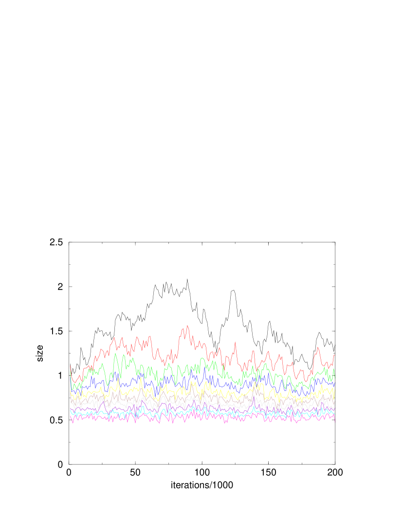
Figure 2: Result of the numerical simulation, where $N=800$ and the number of 8-fold bond is fixed to be 140. The horizontal axis represents the number of iterations, the vertical axis the length of the ten principal axes in ten dimensions. Two of them are relatively large, suggesting the existence of anisotropy in space-time.

In the remainder of this section, we show how we perform numerical simulations. Our conjecture is that a small number of 8-fold bonds fold the branched polymer into four-dimensional space-time. Thus we take the following model:

$$Z=\int\prod_{i=1}^{N-1}d^{10}x^{i}\sum_{G:{\rm maximal\;tree}}\;\;\sum_{B:{\rm sets\;of\;8\mbox{-}fold\;bonds}}e^{-S},$$ (30)

where

$$S = \sum_{(ij)\in G}12\ln[(x^{i}-x^{j})^{2}+1]+\sum_{(ij)\in B}6\ln[(x^{i}-x^{j})^{2}+1]$$ (31)

$$+\sum_{i<j}\theta(1-(x^{ij})^{2})(-4)\ln[(x^{ij})^{2}(2-(x^{ij})^{2}))].$$

Here we fix the number of 8-fold bonds by hand. It is enough to check the above mentioned conjecture, although the number of 8-fold bonds is actually fixed by dynamics.

We generate distribution of $\{x^{i}_{\mu}\}$ by the Monte Carlo method. We then measure moment of inertia,

$$M_{\mu\nu}=\sum_{i=1}^{N}(x^{i}_{\mu}-x^{\rm cm}_{\mu})(x^{i}_{\nu}-x^{\rm cm}_{\nu}),$$

and diagonalize it. The ten eigenvalues are the length squared in the principal axes in ten dimensions. In this way, we analyze anisotropy of ten-dimensional space-time. For example, if four of the eigenvalues are much larger than the others, and grow as we take $N$ large, it means space-time is four-dimensional.

Figure 2 is our preliminary result. In $N=800$, two of the ten eigenvalues are relatively large, suggesting the existence of anisotropy. We hope to see four eigenvalues become larger as we increase $N$. However, in order to see this, we need at least $4^{4}\cdot 2^{6}\sim 16,000$ points, which is quite a large number in the current computer power. Thus, we are trying to make some modifications to the model (31) to study the system with larger $N$. The results will be reported soon. [24]

4 Symmetries in the low energy theory

4.1 Local gauge invariance

Once we describe the space-time as a dynamically generated distribution of the eigenvalues, low-energy effective theory in the space-time can be obtained by solving the dynamics of the fluctuations around the background $X_{\mu}$. Both of the space-time $X_{\mu}$ and matter $\tilde{A}_{\mu}$ are unified in the same matrices $A_{\mu}$ and should be determined dynamically. Low-energy fluctuations are generally composites of $A_{\mu}$ and $\psi$, and it is natural from the analysis of the Schwinger-Dyson equation for the Wilson loops that a local operator in space-time is given by a microscopic limit of the Wilson loop operators, such as

$$w(k;O)={\rm Tr}[O(A,\psi)\exp(ik^{\mu}A_{\mu})].$$ (1)

Here, $O(A,\psi)$ is some operator made of $A_{\mu}$ and $\psi$. In order to identify the total momentum of this operator with $k$, the operator $O(A,\psi)$ should be invariant under a constant shift of $A_{\mu}$, that is, a translation in the space-time coordinates.

In the first approximation around the diagonal background $X_{\mu}$, the coordinate representation of this operator is given by

$$\hat{w}(x;O) = \int{d^{10}k\over(2\pi)^{10}}\exp(-ik^{\mu}x_{\mu})\ w(k;O)$$ (2)

$$\sim \sum_{i=1}^{N}O_{ii}\delta^{(10)}({\boldsymbol{x}}-{\boldsymbol{x_{i}}}).$$

Here, we have replaced $A_{\mu}$ by $X_{\mu}+\tilde{A}_{\mu}$ and taken the leading term. $O_{ii}$ is the $(ii)$ component of the operator $O$. Due to the delta function, the operator has support only in the domain where the eigenvalues distribute. Vanishing of the operator $\hat{w}(x;O)$ outside of the domain of the distributed eigenvalues implies that space-time simply does not exist outside the domain. This fact supports our interpretation of the space-time in IIB matrix model.

We can apply a similar analysis to strings which propagate in the space-time. In the $1/N$ expansion, the correlation between Wilson loop operators can be evaluated by summing over all surfaces made of Feynman diagrams connecting the Wilson loops at the boundary. This surface is interpreted as a string world sheet connecting strings at the boundaries. Each eigenvalue ($x_{\mu}^{i}$) associated to a loop in the diagrams represents a coordinate on the world sheet, and it takes a value in the eigenvalue distribution in the leading approximation around the diagonal background $X_{\mu}$. Hence, a string world sheet evolves only in the space-time of the eigenvalue distribution, which again supports our interpretation of space-time.

It is generally difficult to obtain how fluctuations propagate in the eigenvalue distribution, which is reminiscent of the QCD effective theory: In QCD excitations are expressed as composite operators of microscopic variables, and their low-energy dynamics can be discussed only through a symmetry argument, namely an argument based on chiral symmetry. Also, in our case, we will show that there are eigenvalue distributions around which symmetry arguments allow us to discuss the low-energy dynamics for some excitations. Suppose that the eigenvalue distribution forms clusters consisting of $n$ eigenvalues. At a length scale much larger than the size of each cluster, the $SU(N)$ symmetry is broken down to $SU(n)^{m}$, where $m=N/n$.

We can expand $A_{\mu}$ and $\psi$ around such a background $X_{\mu}$ similarly to the analysis in the previous section. First, write $A_{\mu}$ and $\psi$ in block forms:

$$A_{\mu} = \left(\begin{array}[]{llll}A_{\mu}^{11}&A_{\mu}^{12}&...&\\ A_{\mu}^{21}&A_{\mu}^{22}&&\\ \vdots&&\ddots&\\ &&&A_{\mu}^{mm}\end{array}\right),$$ (7)

$$\psi = \left(\begin{array}[]{llll}\psi^{11}&\psi^{12}&...&\\ \psi^{21}&\psi^{22}&&\\ \vdots&&\ddots&\\ &&&\psi^{mm}\end{array}\right).$$ (12)

Each block, $A_{\mu}^{ij}$ or $\psi^{ij}$, is an $n\times n$ matrix, and the diagonal blocks can be further decomposed:

$$A_{\mu}^{ii} = x_{\mu}^{i}{\bf 1}+\tilde{A}_{\mu}^{ii},$$

$$\psi^{ii} = \xi^{i}{\bf 1}+\tilde{\psi}^{ii},$$ (13)

where ${\bf 1}$ is an $n\times n$ unit matrix and tr $\tilde{A}_{\mu}^{ii}=0$. Here, tr means the trace for a submatrix of $n\times n$. We interpret each cluster of the eigenvalues as being a space-time point with an internal structure $SU(n)$. Since each $SU(n)$ symmetry acts on the variables at position $i$ independently, the unbroken $SU(n)^{m}$ symmetry can be regarded as being local gauge symmetry. Indeed, under a gauge transformation of the unbroken $SU(n)^{m}$ symmetry,

$$g=\left(\begin{array}[]{llll}g_{1}&&&\\ &g_{2}&&\\ &&\ddots&\\ &&&g_{m}\\ \end{array}\right)\in SU(n)^{m}\subset SU(N),$$ (18)

the diagonal block fields, $\tilde{A}_{\mu}^{ii}$ and $\tilde{\psi}^{ii}$, transform as adjoint matters, (i.e., site variables in the lattice gauge theory), while the off-diagonal block fields, $A_{\mu}^{ij}$ and $\psi^{ij}$, transform as gauge connections (i.e., link variables):

$$\tilde{A}_{\mu}^{ii}\rightarrow g_{i}\tilde{A}_{\mu}^{ii}g_{i}^{\dagger},$$

$$\tilde{\psi}^{ii}\rightarrow g_{i}\tilde{\psi}^{ii}g_{i}^{\dagger},$$

$$A_{\mu}^{ij}\rightarrow g_{i}A_{\mu}^{ij}g_{j}^{\dagger},$$

$$\psi^{ij}\rightarrow g_{i}\psi^{ij}g_{j}^{\dagger}.$$ (19)

Some of the dynamics for low-energy excitations is governed by this local gauge invariance. Gauge fields live on the links and transform as the link variables in lattice gauge theory. In our case, we have too many such fields (at least 10 boson fields $A_{\mu}^{ij}$ for a link $(ij)$ ), but only one unitary link variable is assured to be massless by the gauge symmetry, and the others acquire mass dynamically. Therefore, in deriving low-energy effective theory, we first apply a polar decomposition to $A_{\mu}^{ij}$ into unitary and hermitian degrees of freedom, and identify all of the unitary components of $A_{\mu}^{ij}$ by setting them to be one common field $U^{ij}$ on each link. We have to integrate those massive off-diagonal block fields $A_{\mu}^{ij}$ while keeping the unitary components $U^{ij}$ and this procedure is performed by the following replacements:

$$\overline{A_{\mu}^{ij}} = 0,$$

$$\overline{A_{\mu}^{ij}\otimes A_{\nu}^{ji}} = g^{2}{\delta_{\mu\nu}\over(x^{ij})^{2}}U^{ij}\otimes U^{ji}.$$ (20)

In the second equation, the factor, $1/(x^{ij})^{2}$, corresponds to the propagation of the hermitian degrees of freedom while the appearance of the link variable $U^{ij}$ corresponds to keeping the unitary degrees of freedom. Higher order correlations can be obtained by using Wick theorem in general except ten-body correlation function for $A_{\mu}^{ij}$. Due to the chiralness of the ten-dimensional fermion, we obtain an extra term proportional to $\epsilon_{\mu_{1}...\mu_{10}}$, coming from fermion one-loop integral.

In order to derive the effective theory for fluctuations around the assumed background, we integrate massive fields first and obtain effective action for other fields as we have obtained the effective action for the diagonal components (i.e., space-time coordinates) in the previous section. Generally speaking, we can expect any terms which are not forbidden by symmetries; supersymmetry and local $SU(n)$ gauge symmetry.

A plaquette action for gauge fields $U^{ij}$ can be generated as follows. The relevant terms in the action are

$$S_{4}={1\over g^{2}}\sum_{i\neq j\neq k\neq l}{\rm tr}(A_{\mu}^{ij}A_{\nu}^{jk}-A_{\nu}^{ij}A_{\mu}^{jk})A_{\mu}^{kl}A_{\nu}^{li}.$$ (21)

By integrating out the hermitian degrees of freedom of the off-diagonal blocks with the procedure (20), this action vanishes; $\bar{S_{4}}=0$. However, interactions generated by $(S_{4})^{2}$ induce a kinetic term for the gauge field:

$$\overline{(S_{4})^{2}}\sim\sum_{i\neq j\neq k\neq l}{g^{4}\over(x^{ij})^{2}(x^{jk})^{2}(x^{kl})^{2}(x^{li})^{2}}{\rm tr}(U^{ij}U^{jk}U^{kl}U^{li}){\rm tr}(U^{il}U^{lk}U^{kj}U^{ji}).$$ (22)

This is the plaquette action generated by a Wilson loop for the adjoint representation, and hence the gauge field $U^{ij}$ indeed propagates in the space-time of the eigenvalue distribution. The gauge field can hop between any pair of space-time points, but the hopping is suppressed by $1/x^{8}$ for distant points and we will recover locality in the continuum limit. Similarly we can obtain a gauge invariant hopping term for adjoint fermion $\psi^{ii}$.

To summarize this subsection, supposing that the distribution of the eigenvalues consists of small clusters of size $n$, we have shown that the low-energy effective theory contains several massless fields, such as the gauge field associated with the local $SU(n)$ gauge symmetry and fermion field in the adjoint representation of $SU(n)$ gauge symmetry. Gauge-invariant kinetic terms were also derived. Our findings are reminiscent of those which are obtained by considering $n$ coincident D9-branes. Presumably our argument here is related to the standard argument of coincident D-branes.

Our system is a lattice gauge theory on a dynamically generated random lattice. It is invariant under a permutation for the set of the $m$ discrete space-time points, since the permutation group $S_{m}$ is a subgroup of the original $SU(N)$ symmetry. The existence of the permutation symmetry is the crucial difference from the ordinary lattice gauge theory on a fixed lattice, which becomes important in deriving the diffeomorphism invariance of our model. We will come back to this point in the next subsection. Although the permutation invariance requires that all space-time points are equivalent, locality in the space-time will be assured due to suppression of the hopping term between distant points. In general, however, we need a sufficient power for the damping of the hopping terms in order to assure locality in the continuum limit. Though we do not yet know the real condition for locality, we expect that terms with lower powers are canceled due to supersymmetry or by averaging over gauge fields.

4.2 Diffeomorphism invariance

As shown in §2, the one-loop effective action for the space-time points is described as a statistical system of $N$ points whose coordinates are $x_{\mu}^{i}$. Integration over the fermion zeromodes $\xi$ gives the Boltzmann weight, which depends on a graph (or network) connecting the space-time points locally by the bond interactions:

$$Z=\sum_{G:{\rm graph}}\int dX\ W[X;G].$$ (23)

$W[X;G]$ is a complicated function of a configuration $X$ and a graph $G$. An important property is that the weight is suppressed at least by a damping factor of $1/(x^{i}-x^{j})^{12}$, when two points, $i$ and $j$, are connected. This system is, of course, invariant under permutations $S_{N}$ of $N$ space-time points, which is a subgroup of the original symmetry $SU(N)$, while the Boltzmann weight for each graph $G$ is not. The invariance is realized by summing over all possible graphs. In other words, the system becomes permutation invariant by rearrangements of the bonds in the network of the space-time points. This reminds us of the dynamical triangulation approach to quantum gravity, [25] where diffeomorphism invariance is believed to arise from summing all possible triangulations. Our system satisfies both the locality and permutation invariance simultaneously by summing over all possible graphs whose points are connected through the local interactions.

Now we see that the permutation invariance of our system actually leads to diffeomorphism invariance. To see how the background metric is encoded in the effective action for low-energy excitations, let us consider, as an example, a scalar field $\phi^{i}$ propagating in distributed eigenvalues. The effective action will be given by

$$S=\sum_{i,j}{(\phi^{i}-\phi^{j})^{2}\over 2}f(x^{i}-x^{j})+\sum_{i}m(\phi^{i})^{2},$$ (24)

where $f(x)$ is a function decreasing sufficiently fast at infinity to assure locality in the space-time. Introducing the density function of the eigenvalues,

$$\rho(x)=\sum_{i}\delta^{(10)}(x-x^{i}),$$ (25)

and a field $\phi(x)$ which satisfies $\phi(x^{i})=\phi^{i}$, the action can be rewritten as

$$S=\int dxdy\langle\rho(x)\rho(y)\rangle{(\phi(x)-\phi(y))^{2}\over 2}f(x-y)+m\int dx\langle\rho(x)\rangle\phi(x)^{2}.$$ (26)

Here, the expectation, $\langle\cdots\rangle$, for the density and the density correlation means that we have taken average over configurations $X$ and networks $G$ of the space-time points.

Normalizing the density correlation in terms of the density,

$$\langle\rho(x)\rho(y)\rangle=\langle\rho(x)\rangle\langle\rho(y)\rangle r(x,y),$$ (27)

and expanding $\phi(x)-\phi(y)=(x-y)_{\mu}\partial^{\mu}\phi(x)+\cdot\cdot\cdot$, the action becomes

$$S = {1\over 2}\int dx\langle\rho(x)\rangle\left[\int dy\langle\rho(y)\rangle(x-y)_{\mu}(x-y)_{\nu}f(x-y)r(x,y)\right]\partial^{\mu}\phi(x)\partial^{\nu}\phi(x)$$ (28)

$$+m\int dx\langle\rho(x)\rangle\phi(x)^{2}\cdots.$$

This expansion shows that the field $\phi(x)$ propagating in the eigenvalue distribution feels the density correlation as the background metric, while the density itself as vacuum expectation value of the dilaton field. Namely, we can identify

$$g_{\mu\nu}(x) \sim \int dy\langle\rho(y)\rangle(x-y)_{\mu}(x-y)_{\nu}f(x-y)r(x,y),$$ (29)

$$\sqrt{g}e^{-\Phi(x)} \sim \langle\rho(x)\rangle.$$ (30)

If the density correlation respects the original translational and rotational symmetry, that is, if they are not spontaneously broken, the metric becomes flat, $g_{\mu\nu}\sim\eta_{\mu\nu}$. (Normalization can be absorbed by the dilaton vev.) The fact that the background metric is encoded in the density correlations indicates that our system is general covariant, even though the IIB matrix model action (1) defined in flat ten dimensions does not have a manifest general covariance.

Then, let us see how the diffeomorphism invariance is realized in our model. The action (1) is invariant under the permutation $S_{N}$ of the eigenvalues, which is a subgroup of $SU(N)$. Under a permutation,

$$x^{i}\rightarrow x^{\sigma(i)}\ \ \mbox{for}\ \ \sigma\in S_{N},$$ (31)

the field $\phi^{i}$ transforms into $\phi^{\sigma(i)}$. Then, from the definition of the field $\phi(x)$, we should extend the transformation (31) into $x$,

$$x\rightarrow\xi(x),$$ (32)

such that $\xi(x^{i})=x^{\sigma(i)}$. Under this transformation, the eigenvalue density transforms as a scalar density and the field $\phi(x)$ as a scalar field. On the other hand, the metric transforms as a second-rank tensor, if the function $f(x-y)$ decreases rapidly around $x=y$ and the $y$ integral in Eq. (29) has support only near $y=x$. The tensor property of the metric is also required from the invariance of the action under transformation (32). In this way, the invariance under a permutation of the eigenvalues leads to the invariance of the low-energy effective action under general coordinate transformations.

The background metric is encoded in the density correlation of the eigenvalues. Since we have started from the IIB matrix model action (1) which is Poincaré-invariant, the density correlation is expected to be translational and rotational invariant, and we may obtain a low-energy effective action in a flat background. A nontrivial background can be induced dynamically if the Lorentz symmetry is spontaneously broken and the eigenvalues are nontrivially distributed.

A nontrivial background can also be described by condensing a graviton opera-tor. [26] Bosonic parts of graviton and dilaton operators are given by

$$S_{\mu\nu}(k) \sim {\rm Tr}(F_{\mu\lambda}{F^{\lambda}}_{\nu}e^{ik\cdot A})+(\mu\leftrightarrow\nu),$$ (33)

$$D(k) \sim {\rm Tr}(F^{2}e^{ik\cdot A}).$$ (34)

Their condensation induces extra terms in the IIB matrix model action,

$$S_{\rm{cond}}=\int dk\left(\sum h^{\mu\nu}(k)S_{\mu\nu}(k)+h(k)D(k)\right).$$ (35)

We can similarly obtain an effective action for fluctuations around a diagonal background from this modified matrix model action. Condensation of dilaton changes the Yang-Mills coupling constant $g$ locally in space-time. Since $g$ is the only dimensionful constant in our model, and thus determines the fundamental length scale, a local change in $g$ leads to a local change in the eigenvalue density. This is consistent with our earlier discussion that the dilaton expectation value is encoded in the eigenvalue density. On the other hand, the condensation of graviton induces an asymmetry of space-time. For a condensation of the $k=0$ graviton mode, it is obvious that the condensation can be compensated by a field redefinition of matrices $A_{\mu}$,

$$A_{\mu}\rightarrow(\delta_{\mu}^{\nu}+h_{\mu}^{\nu})A_{\nu},$$ (36)

and the two models, the original IIB matrix model and the modified one with the $k=0$ graviton condensation, are directly related through the above field redefinition. The density of the eigenvalues is mapped accordingly, and the density correlation is expected to become asymmetric in the modified matrix model. For a more general condensation, if the graviton operator $\hat{S}_{\mu\nu}(x)$ (coordinate representation of Eq. (33)) changes only the local property of the dynamics of the eigenvalues, the density correlation will become asymmetric locally in space-time around $x$, and therefore induces a local change in the background metric.

Our low-energy effective action is formulated as a lattice gauge theory on a dynamically generated random lattice. Since the lattice itself is generated dynamically from matrices, we must sum over all possible graphs. In this way, our system is permutation $S_{N}$ invariant, which is responsible for the diffeomorphism invariance. The background metric is encoded in the density correlation of the eigenvalues, and the low-energy effective action becomes manifestly general covariant. The graviton operator is represented as fluctuation around the background space-time, and is constructed from the off-diagonal components of the matrices. A microscopic derivation of the propagation of the graviton is difficult to obtain, but once we have clarified the underlying diffeomorphism symmetry, it is natural that the low-energy effective action for the graviton is described by the Einstein Hilbert action. By employing this diffeomorphism invariance and the supersymmetry, we will be able to derive the low-energy behavior of the graviton multiplets, which will be reported in a separate paper.

5 Discussion

We have reviewed the current status of the type IIB matrix model, which is proposed as a constructive definition of superstring.

There are still several conceptual issues. We have obtained a nonabelian gauge symmetry from the IIB matrix model by assuming a particular eigenvalue distribution. This indicates that this vacuum is not a perturbative vacuum of the type IIB superstring. Instead, we may wonder if this is a perturbative vacuum of a heterotic string or a type I string realized in a nonperturbative way within the IIB matrix model. As we discussed in the introduction, our matrix model contains both of the world sheets of the fundamental IIB string and those of the D-strings. By a semiclassical correspondence (8), we have identified a IIB superstring in the Schild gauge where tr is interpreted as integration over a D-string world sheet. We can also construct an F-string world sheet in terms of surfaces made of Feynman diagrams, whose $SU(N)$ index represents the space-time coordinate of a world sheet point. In both cases, if we assume an eigenvalue distribution consisting of small clusters, an internal structure appears on the world sheet, and hence current algebra may arise and there is a possibility to describe heterotic string within the type IIB matrix model.

Another issue is how to describe global topology in the IIB matrix model. A simple example is a torus compactification. A possible procedure of torus compactification [28] is to identify $A_{\mu}$ with $A_{\mu}+R_{\mu}$ by embedding a derivative operator into our matrix configuration. Therefore, $N$ is taken as infinity from the beginning. Since this procedure has a subtlety in the large $N$ limit, we require a careful examination of the double scaling limit.

We also do not yet know how we can describe chiral fermions in lower dimensions after compactification. If we naively consider a low energy effective theory on a four-dimensional space-time generated by distributed eigenvalues, we will obtain fermions with both chiralities. A possible mechanism to produce a chiral fermion is to consider a compactified six-dimensional space-time with a nontrivial index, or a parity violating background. We should replace the $n\times n$ block matrices considered in §4 by $(n+\infty)\times(n+\infty)$ matrices. Size $n$ part of a block represents the low energy gauge symmetry as before. The rest of the infinite size represents an internal space with six dimensions, which should have a non-trivial index. For simplicity, let us consider a two-dimensional internal space. Then the following background

$$A_{a}^{ii} = x_{a}^{i}{\bf 1},$$

$$A_{5}^{ii} = \left(\begin{array}[]{ll}0&\\ &P\end{array}\right),$$ (38)

$$A_{6}^{ii} = \left(\begin{array}[]{ll}0&\\ &Q\end{array}\right)$$ (40)

gives the $(ii)$ block components of a desired background. Here $a=1\sim 4$ and $P,Q$ are infinite dimensional matrices satisfying $[P,Q]=-i$. This background is invariant under $U(n)\times U(1)$ in each block and this becomes the local gauge symmetry in four-dimensional space-time. The effective theory for low energy fluctuations around the background are similarly obtained as in §4. All the off-diagonal fields become massive and we integrate them over except a gauge field. In diagonal blocks, there are several fields that can be massless. Writing fluctuations in a diagonal block, $O=\tilde{A}_{\mu}^{ii}$ or $\tilde{\psi}^{ii}$ as

$$O=\left(\begin{array}[]{ll}O_{A}&O_{F}^{\dagger}\\ O_{F}&O_{S}\end{array}\right),$$ (43)

$O_{A}$ transforms as an adjoint representation, $O_{F}^{\dagger}$ as a fundamental representation and $O_{S}$ is a singlet for $SU(n)$ transformation. $P$ or $Q$ acts like $PO_{F}^{\dagger}$ on $O_{F}^{\dagger}$, and $[P,O_{S}]$ on $S$-components. Then we can show that we obtain a massless chiral fermion with fundamental representation for gauge symmetry $SU(n)$, whose wavefunction in $(P,Q)$ space is given by the groundstate wavefunction of a harmonic oscillator. Other possibly massless fermions are vector-like and will acquire mass unless they are protected by supersymmetry. This is the simplest way to obtain a chiral fermion in four-dimensional space-time. In this construction, all non-singlet fields transforming as adjoint or fundamental representations live in four dimensions and localized at $x_{5}=x_{6}=0$. However, singlet fields including graviton propagate in the bulk (here, six dimensions). In order to have a four-dimensional theory, we need to compactify the internal six-dimensional space. This is discussed in a separate paper.

It is also desirable to construct $AdS$ type backgrounds in our approach.[29] Let us recall the metric of $AdS_{5}\times S^{5}$:

$$ds^{2}={R^{2}\over z^{2}}(d\vec{x}^{2}+dz^{2})+R^{2}d\Omega^{2}_{5}.$$ (44)

The volume factor $\sqrt{g}\sim{1\over z^{5}}$ is sharply peaked at $z=0$ in $AdS_{5}$. Since we have argued that $\sqrt{g}$ is proportional to the density distribution in IIB matrix model, such a background may be represented by the eigenvalue distribution which is also sharply peaked at $z=0$ namely at the four-dimensional boundary. The gauge theory is obtained by assuming that the full $SU(N)$ matrices are decomposed into the clusters of submatrices of $SU(n)$ as we have argued. Since the eigenvalue distribution is essentially four-dimensional, the resulting low energy effective theory must be a four-dimensional field theory. If we further assume ${\cal N}=4$ supersymmetry in four dimensions which must be present due to the conformal symmetry of $AdS_{5}\times S^{5}$, we may conclude that the low energy effective theory for such a background of IIB matrix model is ${\cal N}=4$ super Yang-Mills theory.

References

- [1] N. Ishibashi, H. Kawai, Y. Kitazawa and A. Tsuchiya, Nucl. Phys. B498 (1997), 467; hep-th/9612115.
- [2] M. Fukuma, H. Kawai. Y. Kitazawa and A. Tsuchiya, Nucl. Phys. B510 (1998), 158; hep-th/9705128.
- [3] H. Aoki, S. Iso, H. Kawai, Y. Kitazawa and T. Tada, Prog. Theor. Phys. 99 (1998), 713; hep-th/9802085.
- [4] S. Iso and H. Kawai, hep-th/9903217
- [5] T. Banks, W. Fischler, S. H. Shenker and L. Susskind, Phys. Rev. D55 (1997), 5112; hep-th/9610043.
- [6] R. Dijkgraaf, E. Verlinde and H. Verlinde, Nucl. Phys. B500 (1997), 43.
- [7] V. Periwal, Phys. Rev. D55 (1997), 1711; hep-th/9611103.
- [8] T. Yoneya, Prog. Theor. Phys. 97 (1997), 949; hep-th/9703078.
- [9] J. Polchinski, Prog. Theor. Phys. Suppl. No. 134 (1999), 158; hep-th/9903165.
- [10] H. Sugawara, hep-th/9708029.
-
[11]
H. Itoyama and A. Tokura, Prog. Theor. Phys. 99 (1998), 129; hep-th/9708123;
Phys. Rev. D58 (1998), 026002; hep-th/9801084.
B. Chen, H. Itoyama and H. Kihara, hep-th/9810237.
H. Itoyama and A. Tsuchiya, hep-th/9812177.
K. Ezawa, Y. Matsuo and K. Murakami, Phys. Lett. B439 (1998), 29; hep-th/9802164. -
[12]
N. Kim and S. J. Rey, Nucl. Phys. B504 (1997), 189; hep-th/9701139.
T. Banks and L. Motl, hep-th/9703218.
D. A. Lowe, Phys. Lett. B403 (1997), 243; hep-th/9704041.
S. J. Rey, Nucl. Phys. B502 (1997), 170; hep-th/9704158.
P. Horava, Nucl. Phys. B505 (1997), 84; hep-th/9705055.
M. Krogh, Nucl. Phys. B541 (1999), 87, 98; hep-th/9801034, hep-th/9803088. -
[13]
Several variants of type IIB matrix model have
also been proposed:
A. Fayyazuddin, Y. Makeenko, P. Olesen, D. J. Smith and K. Zarembo, Nucl. Phys. B499 (1997), 159, hep-th/9703038.
C. F. Kristjansen and P. Olesen, Phys. Lett. B405 (1997), 45; hep-th/9704017.
J. Ambjorn and L. Chekhov, JHEP 12(1998)007; hep-th/9805212.
S. Hirano and M. Kato, Prog. Theor. Phys. 98 (1997), 1371; hep-th/9708039.
I. Oda, hep-th/9806096, hep-th/9801085; Phys. Lett. B427 (1998), 267; hep-th/9801051.
N. Kitsunezaki and J. Nishimura, Nucl. Phys. B526 (1998), 351.
T. Tada and A. Tsuchiya, hep-th/9903037. -
[14]
T. Eguchi and H. Kawai, Phys. Rev. Lett. 48 (1982), 1063.
G. Parisi, Phys. Lett. 112B (1982), 463.
D. Gross and Y. Kitazawa, Nucl. Phys. B206 (1982), 440.
G. Bhanot, U. Heller and H. Neuberger, Phys. Lett. 113B (1982), 47.
S. Das and S. Wadia, Phys. Lett. 117B (1982), 228.
J. Alfaro and B. Sakita, Phys. Lett. 121B (1983), 339. -
[15]
J. Polchinski, Phys. Rev. Lett. 75 (1995), 4724.
E. Witten, Nucl. Phys. B443 (1995), 85. - [16] M. Green and J. Schwarz, Phys. Lett. 136B (1984), 367.
- [17] A. Schild, Phys. Rev. D16 (1977), 1722.
- [18] M. Green, J. Schwarz and L. Brink, Nucl. Phys. B219 (1983), 437.
-
[19]
I. Chepelev, Y. Makeenko and K. Zarembo, Phys. Lett. B400 (1997), 43;
hep-th/9701151.
A. Fayyazuddin and D.J. Smith, Mod. Phys. Lett. A12 (1997), 1447; hep-th/9701168.
I. Chepelev and A. A. Tseytlin, Nucl. Phys. B511 (1998), 629; hep-th/9705120.
B. P. Mandal and S. Mukhopadhyay, Phys. Lett. B419 (1998), 62; hep-th/9709098.
N. D. Hari Dass and B. Sathiapalan, Mod. Phys. Lett. A13 (1998), 921; hep-th/9712179.
Y. Kitazawa and H. Takata, hep-th/9810004.
N. Hambli, hep-th/9812008. - [20] K. Hamada, Phys. Rev. D56 (1997), 7503; hep-th/9706187.
-
[21]
See Ref. \citenAIKKT and
T. Hotta, J. Nishimura and A. Tsuchiya,
hep-th/9811220.
T. Nakajima and J. Nishimura, Nucl. Phys. B528 (1998), 355; hep-th/9802082.
W. Krauth and M. Staudacher, hep-th/9902113 for numerical analysis of eigenvalue distribution.
For an evaluation of the partition function:
W. Krauth, H. Nicoli and M. Staudache, Phys. Lett. B431 (1998), 31; hep-th/9803117.
W. Krauth and M. Staudacher, Phys. Lett. B435 (1998), 350; hep-th/9804199.
S. Bal and B. Sathiapalan, hep-th/9902087. -
[22]
A. Connes,
Commun. Math. Phys. 182 (1996), 155; hep-th/9603053.
A. Connes, M. Douglas and A. Schwarz, JHEP 02(1998)003; hep-th/9711162. -
[23]
M. Green and M. Gutperle, JHEP 01(1998)005; hep-th/9711107;
Phys. Rev. D58 (1998), 046007; hep-th/9804123.
G. Moore, N. Nekrasov and S. Shatashvilli, hep-th/9803265.
V. A. Kazakov, I. K. Kostov and N. A. Nekrasov, hep-th/9810035.
P. Vanhove, hep-th/9903050.
F. Sugino, hep-th/9904122.
Also see papers in Ref. \citennumerical. - [24] H. Aoki, H. Kawai and T. Nakajima, in preparation.
- [25] J. Ambjorn, B Durhuus and T. Jonsson, Quantum Geometry (Cambridge, 1997).
-
[26]
Condensation of graviton is discussed in the paper by Yoneya
from a slightly different point of view:
T. Yoneya, Prog. Theor. Phys. Suppl. No. 134 (1999), 182; hep-th/9902200. -
[27]
T. L. Kaluza, Sitz. Bal. Akad. (1921), 966.
O. Klein, Z. Phys. 37 (1926), 895.
Also see recent discussions, F. Wilczek, Phys. Rev. Lett. 80 (1998), 4851; hep-th/9801184. - [28] W. Taylor, Phys. Lett. B394 (1997), 283; hep-th/9611042.
-
[29]
J. Maldacena, Adv. Theor. Math. Phys. 2 (1998), 231.
S. S. Gubser, I. R. Klebanov and A. M. Polyakov, Phys. Lett. B428 (1998), 105.
E. Witten, Adv. Theor. Math. Phys. 2 (1998), 253.