CERN-TH/99-211 hep-th/9908024

BACK-REACTION TO DILATON-DRIVEN INFLATION

A. Ghosh, R. Madden, G. Veneziano

CERN, Theory Division

CH-1211, Geneva 23

We compute the leading-order back-reaction to dilaton-driven inflation, due to graviton, dilaton and gauge-boson production. The one-loop effect turns out to be non-vanishing (unlike the case for pure de-Sitter and for power-law inflation), to be of relative order $\ell_{P}^{2}H^{2}(t)$, and to have the correct sign for favouring the exit to a FRW phase.

CERN-TH/99-211

1 Introduction

In recent years, pre-big bang (PBB) cosmology [1] has established itself as a logically consistent alternative to standard slow-roll inflation [2]. While the ultimate verdict on which, if either, of these two versions of cosmology will survive is left to future experiments, at the theoretical level each one has its own advantages and shortcomings.

The trade-off follows from the fundamental physical difference between the two scenarios: in slow-roll inflation the evolution is from larger to smaller curvatures, while in dilaton-driven PBB inflation the opposite is true. Thus, while in the former case Planckian/string-scale curvatures are naturally reached at the very beginning, pushing the problem of initial conditions into the full quantum-gravity domain (see e.g. [3]), in the latter that problem can be tackled within a perfectly known (albeit non-linear) set of equations (see e.g. [4]). On the other hand, since large curvatures naturally occur at the end of dilaton-driven inflation, the exit problem becomes harder to analyse than in the conventional scenario.

It is generally believed that the exit problem of string cosmology [5], i.e. achieving a smooth, non-singular transition from inflationary to FRW-type string cosmology solutions, should be solved by a combination of two kinds of effects, corresponding to two different classes of corrections to the low-energy, tree-level effective action. While higher-derivative corrections should be able to bound the growth of curvature [6] (or to allow a reinterpretation of the lowest-order curvature singularity), loop corrections [7], accounting for the back-reaction on the geometry from particle production, should stop the growth of the coupling (of the dilaton) when a certain critical-energy condition [8] is reached. Recent proposals of cosmological entropy bounds [9] appear to support [10] these ideas.

Unfortunately, present techniques are still inadequate for giving a convincing answer to the question of whether any one of these desired effects does actually take place. The question of fully non-perturbative higher-derivative corrections amounts to finding an exact (2D) conformal field theory. However, since supersymmetry is spontaneously broken in the case of cosmology, chances to get such a CFT in closed form are slim.

Similarly, understanding the full effect of back-reaction would require knowledge of the full one-loop effective action up to four derivatives. In spite of brilliant work by Vilkovisky and collaborators [11] on this problem, these are still early times for applying the results so far obtained to our problem. Thus our aim here will be more modest: we will try to understand in which direction does the back-reaction from particle production work in PBB cosmology while it is still a small effect. No attempt will be therefore be made to achieve (a fortiori to describe) a complete exit.

We thus took an easier road, recently opened by Iliopoulos et al. [12] and by Abramo and Woodard [13], [14]. Their method was already checked, whenever possible, against the more intuitive approach of Abramo, Brandenberger and Mukhanov [15]. Apart from our use of a different gauge, known to be more appropriate in string cosmology, our work can be seen as a straightforward application of that method in the context of string cosmology. As a check of gauge invariance, we will also reproduce some results of [13], [14].

Another (apparently strong) limitation of our work is that we consider loop corrections to solutions of the low-energy effective action, i.e. we do not include higher-derivative terms in the latter. Since the back-reaction effect turns out to be of the same order as a four-derivative term, it may look suspicious to neglect such terms in the tree-level action while keeping them in the correction. There is, however, a limit in which such an approximation is justified: it is a large-$N$ limit, where $N$ is the number of species of the produced particles. The one-loop back-reaction is of relative order $g^{2}N\ell_{s}^{2}R$ and thus dominates over a tree-level higher-derivative correction ${\cal O}(\ell_{s}^{2}R)$ at sufficiently large $g^{2}N$. Finally, it can also be shown that higher-loop effects on the metric, the dilaton and the antisymmetric tensor (axion) are parametrically smaller at large $g^{2}N$ and small $g^{2}$, justifying the one-loop approximation. This observation makes it all the more urgent to devote further effort to a non-perturbative understanding of one-loop back-reaction in cosmology.

The paper is organized as follows: after recalling (Sections 2 and 3) the form of the lowest-order PBB background whose modification we wish to compute, and the general idea of the method, we will introduce (Section 4) our gauge choice and then go, in Section 5, to the heart of the calculation of the back-reaction, first from gravi-dilaton production, and then from gauge-bosons production. In Section 6, after expressing the final result in a convenient form, we will argue that the back-reaction is of the expected order of magnitude and that, at leading order at least, it modifies the original background in the right direction to help with the exit problem. Finally, an explicit check of the gauge independence of our results is presented in an Appendix.

2 PBB Backgrounds and Fluctuations

In units in which $16\pi G=\hbar=c=1$ the normalized four-dimensional gravi-dilaton effective action in the Einstein frame reads:

$$S=\int d^{4}x\sqrt{-g}\left[R-{1\over 2}(\nabla\varphi)^{2}\right]\;.$$ (2.1)

Even within this minimal set of moduli (corresponding to having frozen the axion as well as internal dimensions), the gravi-dilaton system offers several interesting cosmological solutions, including, of course, the simplest ones, which describe spatially flat, homogeneous and isotropic Universes. In the comoving (cosmic)-time frame the line element takes the form

$$ds^{2}=-dt^{2}_{0}+a_{0}^{2}(t_{0})\,d{\boldmath\vec{x}}\cdot d{\boldmath\vec{x}}\;,$$ (2.2)

where $t_{0}$ represents comoving time (we shall often use the suffix $0$ to denote tree-level quantities). In the discussion of quantum fluctuations it is often convenient to go over to the so-called conformal frame, in which the metric (2.2) becomes

$$ds^{2}=\Omega^{2}(\eta)\left(-d\eta^{2}+d{\boldmath\vec{x}}\cdot d{\boldmath\vec{x}}\right)\;.$$ (2.3)

We recall that comoving and conformal times are related by $dt_{0}=\Omega d\eta$ . In the conformal frame a typical PBB-type solution appears as follows:

$$\Omega=\left({\eta\over\eta_{\,i}}\right)^{1/2},\qquad\varphi_{0}=-\sqrt{3}\ln\left(-\eta\right)\,,\qquad\eta_{\,i}<\eta<0\;,$$ (2.4)

where, by identifying the (arbitrary) constant $\eta_{\,i}$ with the beginning of dilaton-driven inflation (DDI), we have normalized $\Omega$ to $1$ at that moment. It is convenient to define, as usual, ${\cal H}(\eta)=\Omega^{\prime}/\Omega=1/2\eta$ , which is related to the physical Hubble parameter $H$ by

$$H_{0}={\dot{a}_{0}\over a_{0}}={\Omega^{\prime}\over\Omega^{2}}=H_{i}\Omega^{-3}={1\over 3t_{0}}\,,\qquad t_{0}<0\;,$$ (2.5)

where $H_{i}=1/2\eta_{\,i}$ refers to the initial value of the physical Hubble parameter. Note that, at initial time $\eta=\eta_{i}$, the physical Hubble parameter is given by $\Omega^{\prime}$ since $\Omega_{i}=1$.

We remind the reader that the above background corresponds to DDI in the string frame, with a string-frame scale factor blowing up like $(-t_{s})^{-1/\sqrt{3}}$ when the comoving string time $t_{s}$ approaches $0$ from negative values $(t_{s}\to 0^{-})$. In the Einstein frame, this is seen as a contraction (gravitational collapse, see [4]). What remains frame-independent is the fact that curvature grows in time, rather than decreases as in power-law inflation. This is why the results of [14] cannot be directly used in our context.

Let us now define the fluctuations around the classical backgrounds by:

$$g_{\mu\nu}=\Omega^{2}\left(\eta_{\mu\nu}+\psi_{\mu\nu}\right)\,,\qquad\varphi=\varphi_{0}+\phi\;.$$ (2.6)

Our goal here is to compute the back-reaction on the above homogeneous backgrounds (2.4) (i.e. $\psi_{\mu\nu}$ and $\phi$) due to quantum fluctuations at leading order. Following [13], [14], we will thus parametrize the correction to the solution (2.4) by

$$\langle\psi_{\mu\nu}\rangle = A(\eta)\bar{\eta}_{\mu\nu}+C(\eta)t_{\mu}t_{\nu}$$

$$\langle\phi\rangle = D(\eta)~{}~{},$$ (2.7)

where $t_{\mu}\equiv(-1,0,0,0)$ is a time-like vector and $\bar{\eta}_{\mu\nu}=\eta_{\mu\nu}+t_{\mu}t_{\nu}\equiv{\rm diag}\,(0,1,1,1)$ . In the next section we shall recall the method of Refs. [12], [13], [14] for computing $A,C$ and $D$. Here we just conclude by recalling that $A,C$ and $D$ have no physical meaning separately. For instance, if $A$ and $D$ are given in terms of $C$ by

$$A = {{\cal H}_{0}\over\Omega}(\eta)\int^{\eta}d\eta^{\prime}(\Omega C)(\eta^{\prime})$$

$$D = {1\over 2}{\varphi_{0}^{\prime}\over\Omega}(\eta)\int^{\eta}d\eta^{\prime}(\Omega C)(\eta^{\prime})~{}~{},$$ (2.8)

then all three can be gauged away by the redefinition of time, $\eta\to\eta+{1\over 2}\Omega^{-1}\int^{\eta}\Omega C$.

3 The Procedure

Since our background is of the power-law (though not of the power-inflation) type, we shall closely follow here the procedure described in [14] for computing $A,C,D$. We will then stress at which point the two procedures start to diverge. In [14] the authors first compute some amputated one-point functions denoted by $\alpha,\gamma$ and $\delta$ (see below), and then attach external leg propagators in order to reconstruct the desired functions $A,C,D$. Let us describe the procedure in a different, perhaps simpler, way.

If, generically, we wish to compute a fluctuation $\Psi_{i}$ over a generic background $\Psi_{0i}$, then the relevant one-point function is given by the obvious functional integral

$$\langle\Psi_{i}(x)\rangle={\int D\Psi_{\ell}e^{iS[\Psi_{0\ell}+\Psi_{\ell}]}\Psi_{i}(x)\over\int D\Psi_{\ell}e^{iS[\Psi_{0\ell}+\Psi_{\ell}]}}\;.$$ (3.1)

If the action is expanded only up to the quadratic order in $\Psi_{\ell}$, the one-point functions are trivially zero. If, however, the action is expanded up to cubic order, $S[\Psi_{0\ell}+\Psi_{\ell}]=S[\Psi_{0\ell}]+S_{2}^{ij}[\Psi_{0\ell}]\Psi_{i}\Psi_{j}+S_{3}^{ijk}[\Psi_{0\ell}]\Psi_{i}\Psi_{j}\Psi_{k}$ (the summation convention is adopted everywhere), and $S_{3}^{ijk}[\Psi_{0\ell}]$ is treated perturbatively, then there is a non-trivial one-loop correction to the one-point functions (see Fig. 1). This is the familiar story of vacuum-shifting tadpoles in quantum field theory. Analytically the result can be expressed as follows:

$$\langle\Psi_{i}(x)\rangle={\int D\Psi_{\ell}e^{iS[\Psi_{0\ell}]+iS_{2}^{ij}[\Psi_{0\ell}]\Psi_{i}\Psi_{j}}iS_{3}^{jkn}[\Psi_{0\ell}]\Psi_{i}(x)\Psi_{j}\Psi_{k}\Psi_{n}+...\over\int D\Psi_{\ell}e^{iS[\Psi_{0\ell}]+iS_{2}^{ij}[\Psi_{0\ell}]\Psi_{i}\Psi_{j}}}\;.$$ (3.2)

The calculation of the diagrams in Fig. 1

Figure 1: The one-point functions from tadpoles

can be performed in two steps. First, we compute the amputated one-point function for all possible three-point vertices, $iS_{3}^{jkn}$. Then the full one-point functions are obtained by attaching the appropriate external lines. Formula (3.2) gives

$$\langle\Psi_{i}(x)\rangle=\int d^{4}z\langle\Psi_{i}(x)\Psi_{j}(z)\rangle\langle\Psi_{k}(z)\Psi_{n}(z)\rangle[iS_{3}^{jkn}]\;,$$ (3.3)

where (dropping indices hereafter), $\langle\Psi(x)\Psi(z)\rangle$ is the standard Feynman propagator for the quadratic action $S_{2}[\Psi_{0}]\Psi^{2}\equiv\Psi\Delta\Psi$, i.e.

$$\Delta(x)\langle\Psi(x)\Psi(z)\rangle=i\delta^{4}(x-z)\;.$$ (3.4)

Finally, one can express the one-point function as:

$$\langle\Psi(x)\rangle=-\Delta^{-1}(x)\langle\Psi(x)\Psi(x)\rangle[S_{3}]\;.$$ (3.5)

It turns out that the coincident limit propagator $\langle\Psi(x)\Psi(x)\rangle$ is a function of time, $x^{0}$, only. Therefore, if one can invert the kinetic operator in the zero-momentum limit, then (3.5) provides our final expression for the one-point function. For the purpose of the first step it is convenient to distinguish three kinds of amputated one-point functions, $\alpha$, $\gamma$ and $\delta$, defined respectively in Figs. 2, 3 and 4.

As an illustration of the use of (3.5), we present here the calculation of the one-point function $A$ in the covariant gauge introduced in [12]. Note, from (2.7), that $A$ is nothing but the amplitude $\langle\psi_{11}\rangle$, which can be expanded from the general definition (3.3) and Fig. 1, in terms of the amputated one-point functions $\alpha,\gamma$ and $\delta$ as:

$$A\to\langle\psi_{11}\phi\rangle\cdot\delta+\langle\psi_{11}\psi_{\mu\nu}\rangle t^{\mu}t^{\nu}\cdot\gamma+\langle\psi_{11}\psi_{\mu\nu}\rangle\bar{\eta}^{\mu\nu}\cdot\alpha\;.$$ (3.6)

As in (3.5), the external line propagators can be replaced by the inverse of the kinetic operators in the zero-momentum limit. In the covariant gauge of Iliopoulos et al. the Lagrangian can be diagonalized by transforming the variables into suitable linear combinations. The propagators of the original variables can be read off from those of the diagonalized variables by applying the inverse transformation. For a standard power-law-inflation background, $\Omega\sim t^{s}$ with $s>1$, one easily finds

$$\langle\psi_{11}\phi\rangle = -{\sqrt{s}\over s+1}i\Delta_{A}+{\sqrt{s}\over s+1}i\Delta_{C}$$

$$\langle\psi_{11}\psi_{\mu\nu}\rangle t^{\mu}t^{\nu} = {1\over s+1}i\Delta_{A}+{s\over s+1}i\Delta_{C}$$

$$\langle\psi_{11}\psi_{\mu\nu}\rangle\bar{\eta}^{\mu\nu} = \left(-4+{3\over s+1}\right)i\Delta_{A}+{3s\over s+1}i\Delta_{C}$$ (3.7)

where $i\Delta_{A}$ and $i\Delta_{C}$ are particular propagators of the diagonalizing variables. They can be replaced by the inverses of the corresponding kinetic operators in the zero-momentum limit, $1/D_{A}$ and $1/D_{C}$. With this replacement, when (3.7) is plugged back into the expression for the one-point function $A$ in (3.6), we immediately reach the desired expression for $A$:

$$A={1\over D_{A}}\left[-4\alpha+{1\over s+1}(3\alpha+\gamma)-{\sqrt{s}\over s+1}\delta\right]+{1\over D_{C}}\left[{s\over s+1}(3\alpha+\gamma)+{\sqrt{s}\over s+1}\delta\right]\;.$$ (3.8)

This equation is the same as was given in [14]. The above outline shows how simply the relevant formulae can be obtained once the general result (3.5) has been derived. In the Iliopoulos et al. gauge, which does need ghosts, there are three different types of loops, shown in Figs. 2, 3, and 4, where the dotted line describes the graviton, the dashed line the ghost, and the solid line the dilaton.

Figure 2: The $\alpha$-type amputated one-point function

Figure 3: The $\gamma$-type amputated one-point function

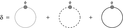
Figure 4: The $\delta$-type amputated one-point function

Let us now briefly compare this approach to the one of Ref. [15], whose authors have used a more intuitive method by computing the energy-momentum tensor of the quantum fluctuations and their back-reaction over the original backgrounds directly. The quantum fluctuations are obtained by solving the linear order perturbation equations and the constraints. In our approach, as in [13], one uses instead the constraints and the gauge-fixing conditions to obtain the Feynman propagators entering the loops. In [15] the back-reaction was computed through systematic corrections of Einstein’s equations, the first non-vanishing correction being quadratic in the Planck length $\ell_{P}$, the small expansion parameter characterizing quantum fluctuations to leading order. The counterpart to this in our approach is that the same parameter, $\ell_{P}^{2}$, controls the loop expansion in quantum gravity. Incidentally, this last observation neatly solves an apparent paradox: classical gravitational waves always carry positive energy while, as we shall see, the back-reaction from the quantum production of gravitational waves from the vacuum turns out to have, at least in some cases, negative energy. The point is that, in the case of the amplification of vacuum fluctuations, there is no parameter allowing a separation of real-graviton production from other virtual one-loop effects whose sign is undetermined. This a-priori non-determination of the sign of the back-reaction is self-evident in the effective action approach [11].

We will follow the same procedure as outlined above in a different gauge where physical variables are more explicit. The usefulness of this gauge was first pointed out in [16] and its significance has been explored in detail in [17], in the context of linear order perturbations to PBB backgrounds. In the next section we summarize results in the off-diagonal gauge relevant for the background (2.4). In the Appendix we will comment on the gauge dependence of the results by comparing them to those obtained in other gauges, e.g. in the covariant gauge of [12].

4 Propagators in the off-diagonal gauge

As explained in the previous section, in order to analyse the perturbations we need to expand (2.1) to quadratic and cubic orders in the fluctuations. We find:

$$\!\!\!\!\!\!\!\!\!S=\int d^{4}x\sqrt{-g}\bigg{[}{g}^{\alpha\beta}{g}^{\rho\sigma}{g}^{\mu\nu}\bigg{\{}\frac{1}{2}\psi_{\alpha\rho,\mu}\psi_{\nu\sigma,\beta}-\frac{1}{2}\psi_{\alpha\beta,\rho}\psi_{\sigma\mu,\nu}+\frac{1}{4}\psi_{\alpha\beta,\rho}\psi_{\mu\nu,\sigma}$$

$$\!\!\!\!\!\!-\frac{1}{4}\psi_{\alpha\rho,\mu}\psi_{\beta\sigma,\nu}\bigg{\}}\Omega^{4}-\frac{1}{2}{g}^{\rho\sigma}{g}^{\mu\nu}\psi_{\rho\sigma,\mu}\psi_{\nu}^{~{}\alpha}(\Omega^{2})_{,\alpha}-{\varphi^{\prime}_{0}}\partial_{\nu}\phi\,g^{0\nu}-\frac{1}{2}\partial_{\mu}\phi\,\partial_{\nu}\phi\,g^{\mu\nu}\bigg{]}$$ (4.1)

Here the ‘pseudo-graviton’ ($\psi_{\mu\nu}$) indices are raised and lowered by $\eta_{\mu\nu}$. To complete the expansion of the $g_{\mu\nu}$ fields in terms of the background and the pseudo-graviton, we recall the expansions

$$g^{\mu\nu} = \Omega^{-2}(\eta^{\mu\nu}-\psi^{\mu\nu}+\psi^{\mu\sigma}\psi_{\sigma}^{\nu}+...)$$

$$\sqrt{-g} = \Omega^{4}\left[1+\frac{1}{2}\psi+(\frac{1}{8}\psi^{2}-\frac{1}{4}\psi^{\alpha\beta}\psi_{\alpha\beta})+...\right]~{},$$ (4.2)

where $\psi=\psi^{\mu}_{\mu}$.

Following [18] we split the fluctuations into tensor and scalar parts by

$$\psi_{\mu\nu}=\left(\matrix{0&0\cr 0&h_{ij}\cr}\right)+\left(\matrix{2\Phi&-\partial_{i}B\cr-\partial_{i}B&2(\Psi\delta_{ij}-\partial_{i}\partial_{j}E)}\right)~{},$$ (4.3)

where $h_{ij}$ represents the (transverse and traceless) tensor part with $h_{ii}=0$ and $\partial_{i}h_{ij}=0$. The trace $\psi$ is given by $\psi=-2\Phi+6\Psi-2\nabla^{2}E$, where $\nabla^{2}\equiv\partial_{i}\partial_{i}$. The action (2.1), when expanded up to quadratic order in the variables (4.3), shows that $B$ and $\Phi$ behave like Lagrange multipliers, giving rise to the following constraints (a prime refers to $\partial/\partial\eta$):

$$B : \quad\Psi^{\prime}+{\cal H}\Phi+{1\over 4}\varphi^{\prime}_{0}\phi=0$$

$$\Phi : \quad 4\nabla^{2}\Psi-12{\cal H}\Psi^{\prime}+\varphi^{\prime}_{0}\phi^{\prime}-4{\cal H}\nabla^{2}(B-E^{\prime})=0\;.$$ (4.4)

Making use of the first constraint in (4.4), it is possible to diagonalize the quadratic part of the action in our background as

$$S_{2}={1\over 2}\int d^{4}x\left[\Big{(}v^{\prime}v^{\prime}-\partial_{i}v\partial_{i}v+{\Omega^{\prime\prime}\over\Omega}v^{2}\Big{)}+{1\over 2}\Big{(}\zeta^{\prime}_{ij}\zeta^{\prime}_{ij}-\partial_{k}\zeta_{ij}\partial_{k}\zeta_{ij}+{\Omega^{\prime\prime}\over\Omega}\zeta_{ij}\zeta_{ij}\Big{)}\right]\;,$$ (4.5)

where $v$ and $\zeta_{ij}$ are the canonical variables, given in terms of the original fields as

$$v=\Omega(\phi-{\varphi^{\prime}_{0}\over{\cal H}}\Psi)=\Omega(\phi+2\sqrt{3}\Psi)\,,\qquad\zeta_{ij}=\Omega h_{ij}\;.$$ (4.6)

Owing to two local gauge symmetries that preserve the form (4.3), two out of the four functions can be fixed through two independent gauge choices. The off-diagonal gauge corresponds to choosing $\Psi=E=0$, which simplifies the first canonical variable to $v=\Omega\phi$. The rest of the variables become related to this canonical variable in simple ways because of other relations following from the constraints (4.4), $\Phi=\sqrt{3}\phi/2$ and $\nabla^{2}B=-\sqrt{3}\phi^{\prime}/2$.

The process of obtaining the propagator for the canonical variables is simplified by dragging the scale factor, $\Omega$, from the canonical variables to the quadratic differential operator. In the off-diagonal gauge this amounts to

$$S_{2}={1\over 2}\int d^{4}x\left[\phi\Delta\phi+{1\over 2}h_{ij}\Delta h_{ij}\right]\,,\qquad\Delta=\Omega\left[-\partial_{\eta}^{2}+\nabla^{2}+{\Omega^{\prime\prime}\over\Omega}\right]\Omega.$$ (4.7)

The differential operator $\Delta$, in the zero-momentum limit, is easily inverted:

$$\Delta^{-1}_{0}f(\eta)\equiv-\int_{\eta_{i}}^{\eta}d\eta_{1}\Omega^{-2}(\eta_{1})\int_{\eta_{i}}^{\eta_{1}}d\eta_{2}f(\eta_{2})\,,\quad\Delta_{0}=\Omega\left[-\partial_{\eta}^{2}+{\Omega^{\prime\prime}\over\Omega}\right]\Omega,$$ (4.8)

as has been advertised in [14]. This choice of the inverse operator also enforces the boundary conditions

$$\Delta^{-1}_{0}f(\eta_{i})=(\Delta^{-1}_{0}f)^{\prime}(\eta_{i})=0,$$ (4.9)

a property we require for the corrections $A$, $C$ and $D$.

From the quadratic action (4.7) it is easy to read out the Feynman propagators for the physical modes

$$\langle\phi(x)\phi(y)\rangle = i\Delta^{-1}(x,y)$$

$$\langle h_{ij}(x)h_{kl}(y)\rangle = 2T_{ijkl}\left[i\Delta^{-1}(x,y)\right]\;,$$ (4.10)

where $T_{ijkl}$ is an appropriately normalized tensor enforcing the transverse and traceless conditions on gravitons, i.e. $\partial_{i}T_{ijkl}=\partial_{j}T_{ijkl}=\partial_{k}T_{ijkl}=\partial_{l}T_{ijkl}=0$ and $T_{iikl}=T_{ijkk}=0$. For our purpose we are interested in computing the propagator $\Delta^{-1}(x,y)$ in the coincident limit $x\to y$. To do this we go to the Fourier-transformed variables

$$\phi(x)=\int{d^{3}k\over(2\pi)^{3}}\phi_{\bf k}(\eta)e^{i{\bf k\cdot x}}\,,\qquad h_{ij}(x)=\int{d^{3}k\over(2\pi)^{3}}h_{{\bf k}ij}(\eta)e^{i{\bf k\cdot x}}~{}~{},$$ (4.11)

where both the mode functions $\phi_{\bf k}$ and $h_{{\bf k}ij}$ can be obtained by solving the differential equations $\Delta f_{\bf k}(\eta)=0$. The solutions can be expressed in terms of Hankel functions of the second kind. Notice that,  $v=\Omega\phi$  being the canonical variable, one should normalize its modes in the far past, $\eta\to-\infty$, as $1/\sqrt{|}{\bf k}|$. By the large-argument limit of the Hankel function, this completely fixes the modes:

$$f_{\bf k}(\eta)={1\over 2\Omega}\sqrt{\pi\eta}H^{(1)}_{0}(|{\bf k}\eta|)\;.$$ (4.12)

Consequently the propagator in the coincident-point limit takes the form

$$\lim_{x\to y}\langle\phi(x)\phi(y)\rangle = {|\eta|\over 8\pi\Omega^{2}}\int dkk^{2}H^{(1)*}_{0}(k|\eta|)H^{(1)}_{0}(k|\eta|)$$

$$\lim_{x\to y}\langle h_{ij}(x)h_{kl}(y)\rangle = {|\eta|\over 4\pi\Omega^{2}}\int dkk^{2}(\delta_{ik}\delta_{jl}+\delta_{il}\delta_{jk}-\delta_{ij}\delta_{kl}-\delta_{ik}{k_{j}k_{l}\over k^{2}}-\delta_{jl}{k_{i}k_{k}\over k^{2}}$$ (4.13)

$$-\delta_{il}{k_{j}k_{k}\over k^{2}}-\delta_{jk}{k_{i}k_{l}\over k^{2}}+\delta_{kl}{k_{i}k_{j}\over k^{2}}+\delta_{ij}{k_{k}k_{l}\over k^{2}}+{k_{i}k_{j}k_{k}k_{l}\over k^{4}})$$

$$\times H^{(1)*}_{0}(k|\eta|)H^{(1)}_{0}(k|\eta|)\;.$$

Here we have replaced the transverse, traceless $T_{ijkl}$ tensor by its Fourier transform. The integral in (4.13) is in general divergent in the ultraviolet. It should be kept in mind, however, that the present approach should be complemented by a momentum cutoff as a result of the ultraviolet sickness of gravity. We set the cutoff, at any given time, at $k_{max}\sim\Omega|H|$, which corresponds to a wavelength of the order of the Hubble radius. This is also the scale at which the mode functions switch from free plane waves to ‘frozen out’ modes. For modes larger than this wavelength the bosonic contribution dominates its fermionic counterpart (we assume some underlying supersymmetry) as a result of Bose-condensation. This is the effect we are after. For shorter-wavelength modes new degrees of freedom should appear, which would ultimately provide better ultraviolet behaviour, as in superstring theory. We also impose an infrared cutoff coming from a finite duration of dilaton-driven inflation, $k_{min}\sim|H_{i}|$, corresponding to the maximal Hubble radius. In conclusion we restrict momenta in all loops to be in the range: $|H_{i}|\leq k\leq\Omega|H|=|H_{i}|/\Omega^{2}$. At this upper-momentum/short-wavelength cutoff, $\Omega|H|\sim 1/|\eta|$, i.e. our cutoff corresponds to $|k\eta|\sim 1$. Note that, in the off-diagonal gauge, as a result of the constraints, all fields can be expressed in terms of $\phi$. Thus only one type of amputated loops, the $\delta$-type, effectively arises on the right-hand side of (3.5).

5 Computation of the one-point functions

In the first two subsections we shall compute the amputated one-point functions due to graviton, dilaton, and gauge-boson loops. In the last subsection the external zero-momentum propagators will be glued in to reconstruct the full one-point functions.

5.1 Graviton and dilaton loops

To get the three-point vertices we use our expansion of the action (4.1) to cubic order in the fluctuations, $S_{3}$. The results are summarized in tables 1 and 2, showing all the relevant three-point vertices. In table 3 we list all the coincident loops appearing in $\delta$ and their respective contributions to the loop integrals ($x=|k\eta|$). There is another way of doing the same computation, which involves, in general, four types of amputated loops in the off-diagonal gauge (Fig. 5).

Figure 5: All possible types of amputated one-point functions in the off-diagonal gauge. Here the line represents all possible coincident propagators.

The first type of loops, having $h_{ij}$ in the external leg, turn out to be zero, since the loop (see both tables 1 and 2), in the coincident limit, always picks up a factor of $\delta_{ij}$, which gives vanishing contributions because of the tracelessness of $h_{ij}$. The second type of loops, having $\Psi_{0i}$ in the external leg, also gives vanishing contributions, but for a different reason. Note that $\Psi_{0i}=\partial_{i}B$ can be integrated by parts to act on the loop. The loops, however, being functions only of time in the coincident limit (4.13) give zero when hit by a space derivative. Thus only the third and fourth types of loops survive in the off-diagonal gauge, the $\delta$-type and $\gamma$-type loops as defined in Figs. 3 and 4.

1	${1\over 2}H_{i}\partial_{2}^{\alpha_{3}}\eta^{\alpha_{1}\beta_{1}}\eta^{\alpha_{2}\beta_{2}}\psi_{\alpha_{1}\beta_{1}}(1)\psi_{\alpha_{2}\beta_{2}}(2)\psi_{\alpha_{3}\beta_{3}}(3)t^{\beta_{3}}$
2	$-H_{i}\partial_{2}^{\alpha_{3}}\eta^{\alpha_{1}\alpha_{2}}\eta^{\beta_{2}\beta_{1}}\psi_{\alpha_{1}\beta_{1}}(1)\psi_{\alpha_{2}\beta_{2}}(2)\psi_{\alpha_{3}\beta_{3}}(3)t^{\beta_{3}}$
3	$-H_{i}\partial_{2}^{\beta_{1}}\eta^{\alpha_{2}\beta_{2}}\eta^{\beta_{3}\alpha_{1}}\psi_{\alpha_{1}\beta_{1}}(1)\psi_{\alpha_{2}\beta_{2}}(2)\psi_{\alpha_{3}\beta_{3}}(3)t^{\alpha_{3}}$
4	${1\over 4}\Omega^{2}\partial_{2}^{\beta_{3}}\partial_{3}^{\alpha_{2}}\eta^{\alpha_{1}\beta_{1}}\eta^{\beta_{2}\alpha_{3}}\psi_{\alpha_{1}\beta_{1}}(1)\psi_{\alpha_{2}\beta_{2}}(2)\psi_{\alpha_{3}\beta_{3}}(3)$
5	$-\Omega^{2}\partial_{2}^{\beta_{3}}\partial_{3}^{\alpha_{1}}\eta^{\beta_{1}\alpha_{2}}\eta^{\beta_{2}\alpha_{3}}\psi_{\alpha_{1}\beta_{1}}(1)\psi_{\alpha_{2}\beta_{2}}(2)\psi_{\alpha_{3}\beta_{3}}(3)$
6	${1\over 2}\Omega^{2}\partial_{2}^{\beta_{3}}\partial_{3}^{\alpha_{2}}\eta^{\beta_{1}\alpha_{3}}\eta^{\beta_{2}\alpha_{1}}\psi_{\alpha_{1}\beta_{1}}(1)\psi_{\alpha_{2}\beta_{2}}(2)\psi_{\alpha_{3}\beta_{3}}(3)$
7	${1\over 4}\Omega^{2}\partial_{2}^{\alpha_{3}}\partial_{3}^{\beta_{3}}\eta^{\alpha_{1}\beta_{1}}\eta^{\alpha_{2}\beta_{2}}\psi_{\alpha_{1}\beta_{1}}(1)\psi_{\alpha_{2}\beta_{2}}(2)\psi_{\alpha_{3}\beta_{3}}(3)$
8	${1\over 2}\Omega^{2}\partial_{2}^{\alpha_{3}}\partial_{3}^{\beta_{3}}\eta^{\alpha_{1}\alpha_{2}}\eta^{\beta_{2}\beta_{1}}\psi_{\alpha_{1}\beta_{1}}(1)\psi_{\alpha_{2}\beta_{2}}(2)\psi_{\alpha_{3}\beta_{3}}(3)$
9	${1\over 2}\Omega^{2}\partial_{2}^{\alpha_{1}}\partial_{3}^{\beta_{3}}\eta^{\alpha_{2}\beta_{2}}\eta^{\beta_{1}\alpha_{3}}\psi_{\alpha_{1}\beta_{1}}(1)\psi_{\alpha_{2}\beta_{2}}(2)\psi_{\alpha_{3}\beta_{3}}(3)$
10	${1\over 2}\Omega^{2}\partial_{2}^{\alpha_{1}}\partial_{3}^{\beta_{2}}\eta^{\alpha_{3}\beta_{3}}\eta^{\beta_{1}\alpha_{2}}\psi_{\alpha_{1}\beta_{1}}(1)\psi_{\alpha_{2}\beta_{2}}(2)\psi_{\alpha_{3}\beta_{3}}(3)$
11	${1\over 8}\Omega^{2}\partial_{2}^{\alpha_{4}}\partial_{3}^{\alpha_{5}}\eta_{\alpha_{4}\alpha_{5}}\eta^{\alpha_{1}\beta_{1}}\eta^{\alpha_{2}\beta_{2}}\eta^{\alpha_{3}\beta_{3}}\psi_{\alpha_{1}\beta_{1}}(1)\psi_{\alpha_{2}\beta_{2}}(2)\psi_{\alpha_{3}\beta_{3}}(3)$
12	${1\over 2}\Omega^{2}\partial_{2}^{\alpha_{4}}\partial_{3}^{\alpha_{5}}\eta_{\alpha_{4}\alpha_{5}}\eta^{\alpha_{1}\alpha_{2}}\eta^{\alpha_{3}\beta_{3}}\eta^{\beta_{2}\beta_{1}}\psi_{\alpha_{1}\beta_{1}}(1)\psi_{\alpha_{2}\beta_{2}}(2)\psi_{\alpha_{3}\beta_{3}}(3)$
13	${1\over 4}\Omega^{2}\partial_{2}^{\alpha_{1}}\partial_{3}^{\beta_{1}}\eta^{\alpha_{2}\beta_{2}}\eta^{\alpha_{3}\beta_{3}}\psi_{\alpha_{1}\beta_{1}}(1)\psi_{\alpha_{2}\beta_{2}}(2)\psi_{\alpha_{3}\beta_{3}}(3)$
14	${1\over 8}\Omega^{2}\partial_{2}^{\alpha_{4}}\partial_{3}^{\alpha_{5}}\eta_{\alpha_{4}\alpha_{5}}\eta^{\alpha_{1}\beta_{1}}\eta^{\alpha_{2}\alpha_{3}}\eta^{\beta_{3}\beta_{2}}\psi_{\alpha_{1}\beta_{1}}(1)\psi_{\alpha_{2}\beta_{2}}(2)\psi_{\alpha_{3}\beta_{3}}(3)$
15	${1\over 2}\Omega^{2}\partial_{2}^{\alpha_{4}}\partial_{3}^{\alpha_{5}}\eta_{\alpha_{4}\alpha_{5}}\eta^{\alpha_{1}\alpha_{2}}\eta^{\beta_{2}\alpha_{3}}\eta^{\beta_{3}\beta_{1}}\psi_{\alpha_{1}\beta_{1}}(1)\psi_{\alpha_{2}\beta_{2}}(2)\psi_{\alpha_{3}\beta_{3}}(3)$
16	${1\over 4}\Omega^{2}\partial_{2}^{\alpha_{1}}\partial_{3}^{\beta_{1}}\eta^{\alpha_{2}\alpha_{3}}\eta^{\beta_{3}\beta_{2}}\psi_{\alpha_{1}\beta_{1}}(1)\psi_{\alpha_{2}\beta_{2}}(2)\psi_{\alpha_{3}\beta_{3}}(3)$

Table 1: List of all $\psi_{\alpha_{1}\beta_{1}}\psi_{\alpha_{2}\beta_{2}}\psi_{\alpha_{3}\beta_{3}}$ vertices. While choosing an external leg one should permute $1,2,3$ in each vertex.

1	$-{\sqrt{3}\over 4}H_{i}\partial_{1}^{\alpha_{6}}\eta^{\alpha_{4}\alpha_{5}}\eta^{\beta_{4}\beta_{5}}\phi(1)\psi_{\alpha_{4}\alpha_{5}}(2)\psi_{\beta_{4}\beta_{5}}(3)t_{\alpha_{6}}$
2	${\sqrt{3}\over 2}H_{i}\partial_{1}^{\alpha_{4}}\eta^{\alpha_{5}\beta_{5}}\eta^{\alpha_{6}\beta_{6}}\phi(1)\psi_{\alpha_{5}\alpha_{6}}(2)\psi_{\beta_{5}\beta_{6}}(3)t_{\alpha_{4}}$
3	$\sqrt{3}H_{i}\partial_{1}^{\alpha_{5}}\eta^{\alpha_{7}\alpha_{8}}\phi(1)\psi_{\alpha_{4}\alpha_{5}}(2)\psi_{\alpha_{7}\alpha_{8}}(3)t^{\alpha_{4}}$
4	$-2\sqrt{3}H_{i}\partial_{1}^{\alpha_{5}}\eta^{\alpha_{6}\alpha_{7}}\phi(1)\psi_{\alpha_{4}\alpha_{6}}(2)\psi_{\alpha_{5}\alpha_{7}}(3)t^{\alpha_{4}}$
5	$-{1\over 4}\Omega^{2}\partial_{1}^{\alpha_{4}}\partial_{2}^{\alpha_{5}}\eta_{\alpha_{4}\alpha_{5}}\eta^{\alpha_{6}\alpha_{7}}\phi(1)\phi(2)\psi_{\alpha_{6}\alpha_{7}}(3)$
6	${1\over 2}\Omega^{2}\partial_{1}^{\alpha_{4}}\partial_{2}^{\alpha_{5}}\phi(1)\phi(2)\psi_{\alpha_{4}\alpha_{5}}(3)$

Table 2: All possible $\phi\psi_{\alpha_{1}\beta_{1}}\psi_{\alpha_{2}\beta_{2}}$ and $\phi\phi\psi_{\alpha_{1}\beta_{1}}$ vertices. Again one should permute appropriate indices when considering each vertex.

$\langle\phi,\phi^{\prime}\rangle$	$\int dxx^{3}H^{(1)*}_{0}(x)H^{\prime(1)}_{0}(x)/16H_{i}\pi|\eta|^{4}$
$\langle\phi,\phi^{\prime\prime}\rangle$	$-\int dxx^{4}H^{(1)*}_{0}(x)H^{\prime\prime(1)}_{0}(x)/16H_{i}\pi|\eta|^{5}$
$\langle\partial_{i}\phi,\partial_{i}\phi\rangle$	$-\int dxx^{4}H^{(1)*}_{0}(x)H^{(1)}_{0}(x)/16H_{i}\pi|\eta|^{5}$
$\langle\partial_{i}\phi,\psi_{0i}\rangle$	$-\sqrt{3}\int dxx^{3}H^{(1)*}_{0}(x)H^{\prime(1)}_{0}(x)/32H_{i}\pi|\eta|^{4}$
$\langle\partial_{i}\phi,\psi^{\prime}_{0i}\rangle$	$\sqrt{3}\int dxx^{4}H^{(1)*}_{0}(x)H^{\prime\prime(1)}_{0}(x)/32H_{i}\pi|\eta|^{5}$
$\langle\partial_{i}\phi^{\prime},\psi_{0i}\rangle$	$\sqrt{3}\int dxx^{4}H^{\prime(1)*}_{0}(x)H^{\prime(1)}_{0}(x)/32H_{i}\pi|\eta|^{5}$
$\langle\psi_{0i},\psi^{\prime}_{0i}\rangle$	$-3\int dxx^{3}H^{\prime(1)*}_{0}(x)H^{\prime\prime(1)}_{0}(x)/64H_{i}\pi|\eta|^{4}$
$\langle\partial_{i}\psi_{0j},\partial_{j}\psi_{0i}\rangle$	$-3\int dxx^{4}H^{\prime(1)*}_{0}(x)H^{\prime(1)}_{0}(x)/64H_{i}\pi|\eta|^{5}$
$\langle\partial_{i}\psi_{0j},\partial_{i}\psi_{0j}\rangle$	$-3\int dxx^{4}H^{\prime(1)*}_{0}(x)H^{\prime(1)}_{0}(x)/64H_{i}\pi|\eta|^{5}$
$\langle\psi_{ij},\psi^{\prime}_{ij}\rangle$	$3\int dxx^{3}H^{(1)*}_{0}(x)H^{\prime(1)}_{0}(x)/8H_{i}\pi|\eta|^{4}$
$\langle\partial_{i}\psi_{jk},\partial_{j}\psi_{ik}\rangle$	$0$
$\langle\partial_{i}\psi_{jk},\partial_{i}\psi_{jk}\rangle$	$-3\int dxx^{4}H^{(1)*}_{0}(x)H^{(1)}_{0}(x)/8H_{i}\pi|\eta|^{5}$
$\langle\phi^{\prime},\phi^{\prime}\rangle$	$-\int dxx^{4}H^{\prime(1)*}_{0}(x)H^{\prime(1)}_{0}(x)/16H_{i}\pi|\eta|^{5}$
$\langle\psi^{\prime}_{ij},\psi^{\prime}_{ij}\rangle$	$-3\int dxx^{4}H^{\prime(1)*}_{0}(x)H^{\prime(1)}_{0}(x)/8H_{i}\pi|\eta|^{5}$

Table 3: All possible coincident loop propagators appearing for the off-diagonal gauge. The prime in $H^{\prime(2)}_{0}$ refers to $\partial/\partial x$, otherwise to $\partial/\partial\eta$.

Another important feature of the off-diagonal gauge is the absence of the Faddeev–Popov ghosts. This can be readily seen from the gauge transformations of the gauge-fixing functions $\Psi$ and $E$. Their gauge transformations have been given in [18]:

$$\Psi\to\Psi+{\cal H}\xi(x)\,,\qquad E\to E-\overline{\xi}(x)\;,$$ (5.1)

where $\xi$ and $\overline{\xi}$ are the two gauge parameters associated with the coordinate transformations: $\eta\to\eta-\xi$ and $x^{i}\to x^{i}-\partial_{i}\overline{\xi}$. Clearly, the Faddeev–Popov determinant is field-independent and hence the ghosts are decoupled, unlike what happens in the covariant gauge of [12].

As an example, we present a sample calculation, say the three-point vertex $\#$5 of table 2. For illustrative purposes, it is easier to make use of the constraints at the beginning (in contrast, in the computer code its more convenient to impose the constraints later). As we have argued, this does not make a difference, which is at the same time an important consistency check for our method. Making use of the constraints in the off-diagonal gauge presented in the previous section, the ${\rm tr}(\psi_{\mu\nu})$, present in the vertex $\#$5, can be replaced by the scalar fluctuation $\phi$. As we said, in this case there is only one type of amputated loop $\delta_{\rm eff}$, that can be read off from the vertex $\#$5:

$$\delta_{\rm eff}={\sqrt{3}\over 4}[-\Omega^{2}\langle\phi^{\prime}\phi^{\prime}\rangle+4H_{i}\langle\phi\phi^{\prime}\rangle+\Omega^{2}\langle\phi\phi\rangle^{\prime\prime}+\Omega^{2}\langle\partial_{i}\phi\partial_{i}\phi\rangle]\;.$$ (5.2)

Now, one should look at table 3, where various propagators have been listed in this gauge and pick up the leading-order terms from (5.2) as we approach the limit, $\eta\to 0^{-}$. Recall that $\Omega^{2}\sim|\eta|$, and hence all the terms in (5.2) are of the same order, $1/\eta^{4}$.

5.2 Gauge-boson loops

Let us now study the back-reaction produced by gauge fields to the background (2.4). There are two distinct types of gauge fields appearing in the low-energy string effective action — the NS-type and the R-type. The NS-type couple to all the fundamental moduli while the R-type couple only to the metric. Let us first concentrate on the NS-type gauge bosons. In the canonical frame the action is:

$$S^{\rm em}={1\over 4}\int d^{4}xe^{-\varphi}\sqrt{-g}g^{\mu\rho}g^{\nu\sigma}F_{\mu\nu}F_{\rho\sigma}\;,$$ (5.3)

which supplements the graviton–dilaton action (2.1) in the presence of the NS-type fields. Since the gauge-boson action (5.3) is already quadratic in the gauge fields, these decouple, to linear order, from other fluctuations. Also, interactions stemming from a possible non-Abelian gauge structure can be ignored. We shall work in the Coulomb gauge where the temporal component of the gauge field is zero and the spatial components satisfy $\partial_{i}A_{i}=0$. Going over to a canonical gauge-field variable, the action can be written in the form

$$S^{\rm em}_{2}={1\over 2}\int d^{4}x\zeta_{i}\overline{\Delta}\zeta_{i}\,,\qquad\overline{\Delta}=-\partial_{\eta}^{2}+\nabla^{2}-e^{\varphi_{0}/2}(e^{-\varphi_{0}/2})^{\prime\prime}\;,$$ (5.4)

where the canonical field is given by $\zeta_{i}=e^{-\varphi_{0}/2}A_{i}$. Fourier expanding as before, the mode functions satisfy the homogeneous equation

$$\zeta_{i}=\int{d^{3}k\over(2\pi)^{3}}\zeta_{{\bf k}i}(\eta)e^{\bf ik\cdot x}\,,\quad\overline{\Delta}\zeta_{i}=0\,,\quad{\bf k}^{i}\zeta_{{\bf k}i}=0\;,$$ (5.5)

the solution of which can be written down [19] in terms of the Hankel functions of the second kind. Following the same normalization arguments as presented before, the Coulomb-gauge Feynman propagator for the canonical fields can be expressed in the form

$$\!\!\!\!\langle\zeta_{i}(x)\zeta_{j}(y)\rangle=\int{d^{3}k\over(2\pi)^{3}}{1\over 4}\Big{(}\delta_{ij}-{k^{i}k^{j}\over k^{2}}\Big{)}\left[\sqrt{\pi\eta}H^{(1)}_{\lambda}(kx^{0})\right]\left[\sqrt{\pi\eta}H^{(1)*}_{\lambda}(ky^{0})\right]e^{i{\bf k\cdot(x-y)}}$$ (5.6)

where the index $\lambda=(\sqrt{3}-1)/2$. The cubic vertices have been listed in table 4 and the coincident loops are presented in table 5.

For the R-type gauge bosons, the coupling to the dilaton being absent in the effective action (5.3), the mode functions satisfy the free wave equations: $\zeta_{{\bf k}i}^{\prime\prime}+k^{2}\zeta_{{\bf k}i}=0$. Clearly, these modes are not parametrically amplified; and hence their contributions to the back-reaction are negligible.

The relevant diagrams for gauge bosons are the same as in Fig. 5 except that here the solid line represents the gauge loop. Notice, from table 4, that all the three-point vertices are quadratic in the gauge fields and at the linear order there is no coupling between the gauge fields and the gravitational perturbations. Among the loops, see again Fig. 5, the ones that have $h_{ij}$ and $\psi_{0i}$ as external legs are zero for the same reason as presented before. The rest of the diagrams are of the $\gamma$ or $\delta$ type. As an example, let us take the vertex $\#$6 of table 4. It contributes to $\delta_{\rm eff}$ as

$$\delta_{\rm eff}={1\over 2}\exp(-\varphi_{0})[-\langle A^{\prime}_{i}A^{\prime}_{i}\rangle+\langle\partial_{k}A_{i}\partial_{k}A_{i}\rangle]\;.$$ (5.7)

The exponential factor is common to all the vertices and is $\sim|\eta|^{\sqrt{3}}$, which cancels the inverse factor in the second coincident-limit propagator, as can be seen from table 5. It requires some more effort to see that this is also happening for the first entry of table 5, but again, even for gauge bosons, the leading effect in the amputated one-point functions is $\sim 1/\eta^{4}$.

1	$-{1\over 4}\exp(-\varphi_{0})\partial_{2}^{\alpha_{5}}\partial_{3}^{\beta_{6}}\eta_{\alpha_{5}\beta_{6}}\eta^{\alpha_{4}\beta_{4}}\eta^{\beta_{5}\alpha_{6}}A_{\beta_{5}}(2)A_{\alpha_{6}}(3)\psi_{\alpha_{4}\beta_{4}}(1)$
2	${1\over 4}\exp(-\varphi_{0})\partial_{2}^{\alpha_{5}}\partial_{3}^{\beta_{5}}\eta^{\alpha_{4}\beta_{4}}A_{\beta_{5}}(2)A_{\alpha_{5}}(3)\psi_{\alpha_{4}\beta_{4}}(1)$
3	${1\over 2}\exp(-\varphi_{0})\partial_{2}^{\alpha_{5}}\partial_{3}^{\beta_{5}}\eta^{\alpha_{6}\beta_{6}}A_{\alpha_{6}}(2)A_{\beta_{6}}(3)\psi_{\alpha_{5}\beta_{5}}(1)$
4	${1\over 2}\exp(-\varphi_{0})\partial_{2}^{\beta_{5}}\partial_{3}^{\alpha_{5}}\eta_{\alpha_{5}\beta_{5}}\eta^{\alpha_{4}\alpha_{6}}\eta^{\beta_{4}\beta_{6}}A_{\alpha_{6}}(2)A_{\beta_{6}}(3)\psi_{\alpha_{4}\beta_{4}}(1)$
5	$-\exp(-\varphi_{0})\partial_{2}^{\alpha_{5}}\partial_{3}^{\beta_{4}}\eta^{\alpha_{4}\beta_{5}}A_{\beta_{5}}(2)A_{\alpha_{5}}(3)\psi_{\alpha_{4}\beta_{4}}(1)$
6	${1\over 2}\exp(-\varphi_{0})\partial_{2}^{\alpha_{5}}\partial_{3}^{\beta_{6}}\eta_{\alpha_{5}\beta_{6}}\eta^{\beta_{5}\alpha_{6}}\phi(1)A_{\beta_{5}}(2)A_{\alpha_{6}}(3)$
7	$-{1\over 2}\exp(-\varphi_{0})\partial_{2}^{\alpha_{5}}\partial_{3}^{\beta_{5}}\phi(1)A_{\beta_{5}}(2)A_{\alpha_{5}}(3)$

Table 4: All possible $\phi A_{\alpha_{1}}A_{\beta_{1}}$ and $\psi_{\alpha_{1}\beta_{1}}A_{\alpha_{2}}A_{\beta_{2}}$ vertices. Again one should permute indices when considering each vertex.

$\langle A^{\prime}_{i_{1}},A^{\prime}_{i_{1}}\rangle$	$\int dxx^{2}[\sqrt{-\eta}(\eta/\eta_{i})^{-\sqrt{3}/2}H^{(1)*}_{\lambda}(|k\eta|)]^{\prime}\;\cdot$
	$[\sqrt{-\eta}(\eta/\eta_{i})^{-\sqrt{3}/2}H^{(1)}_{\lambda}(|k\eta|)]^{\prime}/8\pi|\eta|^{3}$
$\langle\partial_{i_{1}}A_{i_{2}},\partial_{i_{1}}A_{i_{2}}\rangle$	$\int dxx^{4}(\eta/\eta_{i})^{-\sqrt{3}}H^{(1)*}_{\lambda}(x)H^{(1)}_{\lambda}(x)/8\pi|\eta^{4}|$

Table 5: All coincident photon loops. All primes refer to $\partial/\partial\eta$.

5.3 Adding external propagators

Following (3.5) we have first computed the amputated one-point functions in the off-diagonal gauge. As it turned out, after summing over all the vertices in tables 1 and 2, the leading-order terms, as $\eta\to 0$, have the time dependence $1/\eta^{4}$. We now attach the external line, i.e. the inverse of the zero-momentum kinetic operator, $\Delta_{0}$. From (4.8) we note that our amputated quantities have to go through a double $\eta$-integral and multiplication by $\Omega^{-2}$. Thus the leading-order time dependence of the one-point functions is simply $1/\eta^{3}$. Going through the procedure more carefully, we see that, apart for some numerical factors (which are different for different one-point functions), the leading-order contribution to all one-point functions is of order $1/H_{i}\eta^{3}$. This result suggests that, in the context of PBB cosmology, the dominant modes are those near the upper momentum cut-off $k\sim\eta^{-1}$. As we have already argued, contributions from modes beyond this cut-off, $|k\eta|\sim 1$, have to be combined with those from other fields, e.g. from fermions. The resulting combined effect will be typical of a short-distance renormalization of the bare parameters of the Lagrangian, which should be mild in a supersymmetric theory. Apart from this, the physical effect from short distances should be parametrically smaller than the effect we have computed. Considering (2.4), (2.5), and the formula $H_{i}=1/2\eta_{i}$, the contribution we have found can be simply expressed, in our units, as:

$$\left(A,\,C,\,D\right)\sim{1\over H_{i}\eta^{3}}\sim{H_{i}^{2}\over\Omega^{6}}\equiv H_{0}^{2}\;.$$ (5.8)

What about the ratio between the three one-point functions in the off-diagonal gauge? Our answer turns out to be simply:

$$A=0\,,\qquad C=\sqrt{3}D\,,\qquad D=-\Delta^{-1}_{0}\delta_{\rm eff}\;.$$ (5.9)

We should point out that, while (5.9) appears to parametrize only certain forms of metric fluctuations, other contributions, such as $\langle\psi_{0i}\rangle$ or $\langle\psi_{ij}\rangle,\;i\neq j$, have been shown to be exactly zero. Also, the vanishing of $\alpha$ easily follows from the property $h_{ii}=0$ and from the coincident-point limit of the loop (4.13).

To reach (5.9) one could follow another path, which parallels more closely [13] and [14]. One can take into account all types of loops –corresponding to all the variables appearing in the fluctuations (2.6)– and use the constraints at the end. As a matter of fact, this also provides a good consistency check of the method. Here again, from very general considerations (cf. the three-point vertices in tables 1, 2 and 4), loops with $\psi_{0i}$ and $h_{ij}$ as external legs vanish, and only $\delta$-type and the $\gamma$-type amputated functions survive. Thus the results (5.9) follow in a different way:

$$A=0\,,\qquad C=\sqrt{3}D\,,\qquad D=-\Delta^{-1}_{0}\left(\delta+\sqrt{3}\gamma\right)~{}~{},$$ (5.10)

where (5.10) is identical to (5.9) since the constraints provide the relation $\delta_{\rm eff}=\delta+\sqrt{3}\gamma$.

We are now ready to discuss the physical implications of our results for the PBB scenario.

6 Discussion

The physical effects due to back-reaction are best analysed, in a PBB context, by going over to the string frame. In order to prepare for that, let us write down the final outcome of our calculation in the off-diagonal gauge as

$$\langle ds^{2}\rangle = \Omega^{2}[-(1-C)d\eta^{2}+d\vec{x}\cdot d\vec{x}\,]=-dt^{2}+a^{2}(t)d\vec{x}\cdot d\vec{x}$$

$$\langle\varphi\rangle = \varphi_{0}+D\;,$$ (6.1)

where $C$ and $D$ are as given explicitly in (5.10). Since we limit ourselves to times for which $C\ll 1$, the new comoving time $t$ is related to the background comoving time by

$$dt\simeq\Omega\left(1-{1\over 2}C\right)d\eta=\left(1-{1\over 2}C\right)dt_{0}\;.$$ (6.2)

Expressing the dilaton and the Hubble parameter $H$ associated with the scale factor $a$ in the new comoving time, and after using the relation (5.9) between $C$ and $D$ we find

$$\langle\varphi\rangle \simeq -{2\over\sqrt{3}}\left[\ln(-t)-\sqrt{3}D\right]$$

$$H = {d\over dt}\langle\ln a\rangle\simeq{1\over 3t}\left[1+\sqrt{3}D\right]\;.$$ (6.3)

In order to go over to the string frame, we introduce the corresponding comoving time $dt_{s}=\exp(\langle\varphi\rangle/2)dt$ and the scale factor $a_{s}=\exp(\langle\varphi\rangle/2)a$. After a straightforward calculation the resulting string-frame Hubble parameter and dilaton can be written as

$$H_{s} = {d\over dt_{s}}\langle\ln a_{s}\rangle\simeq-{1\over\sqrt{3}t_{s}}\left[1+{{7\sqrt{3}}-3\over 2}D\right]\;,$$

$$\langle\varphi\rangle \simeq -(\sqrt{3}+1)\left[\ln(-t_{s})-(2\sqrt{3}-3)D\right]\;.$$ (6.4)

It turns out that, in the Einstein frame, $D(t)$ is a positive number times the square of the Hubble parameter. For the minimal gravi-dilaton system, we find:

$$D(t)=0.0047H_{0}^{2}(t)\;.$$ (6.5)

Although the coefficient of $H_{0}^{2}$ looks small, we have to recall that, in our units ($16\pi G=\hbar=c=1$), Planck’s time is given by $t_{P}^{2}=1/16\pi$. In other words, the (relative, dimensionless) correction to the tree-level background is:

$$D=0.24\,t_{P}^{2}H_{0}^{2}\;,$$ (6.6)

i.e. does not contain any particularly small number.

When one goes to the string frame, in which the string length $\ell_{s}$ is a constant, the same result as (6.6) for $D$ follows, provided one interprets $t_{P}$ as the effective, time-dependent, Planck time $t_{P}=\ell_{s}e^{\phi/2}$ and $H_{0}$ is expressed in terms of the string-frame Hubble parameter and of $\dot{\phi}$ (now the dot refers to derivative w.r.t. cosmic string time) by the standard relation $H_{0}=H_{s}-\dot{\phi}/2$.

When the NS-gauge-boson loops are included the numbers in (6.5) change but the conclusions do not. The contribution of a single gauge boson to $D$ turns out to be

$$D=0.00016H_{0}^{2}=0.008~{}t_{P}^{2}H_{0}^{2}\;,$$ (6.7)

i.e. of the same sign but about $30$ times smaller than that of the gravi-dilaton system (6.5). The result (6.7) should be multiplied by the number of NS gauge bosons, which, in typical superstring theories, could be in the range of hundreds.

In both cases the one-loop correction adds to the rate of inflation and to the rate of growth of the dilaton. At first sight, this seems to go against an eventual exit from inflation. However, what is crucial for the exit is not so much the absolute rates of growth but rather the relative rate of dilaton and scale-factor growth.

To be more precise, let us compute directly the effect of back-reaction on the string-frame quantity $\dot{\overline{\varphi}}$, where $\overline{\varphi}=\varphi-3\ln a_{s}$ is the duality-invariant shifted dilaton and, as before, the dot refers to the time derivative in the string frame. From Eq. (6.4) we easily compute:

$$\dot{\overline{\varphi}}=-{1\over t_{s}}\left[1-{9-3\sqrt{3}\over 2}D\right]\;.$$ (6.8)

The positive sign of $D$ is forcing $\dot{\overline{\varphi}}$ to decrease (relative to the tree-level value) as the result of a competition between a growing dilaton and a growing Hubble parameter in the string frame. It is thus obvious that the ratio $\dot{\overline{\varphi}}/H_{s}$ will change from its tree-level value of $\sqrt{3}$ towards smaller values. As shown in Fig. 6, this is precisely as required by a graceful exit [5], i.e. the phase-space trajectory in the $\dot{\overline{\varphi}}$-$H$ plane should turn anticlockwise. Incidentally, this is also what the Hubble entropy bound of [9] requires [10].

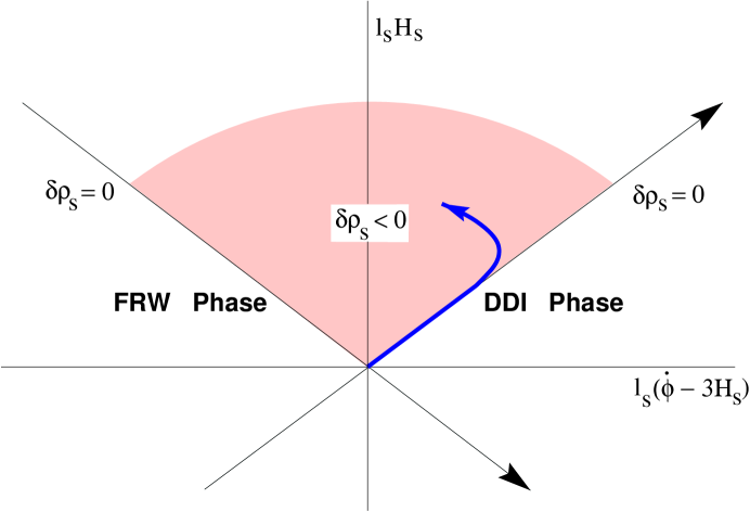
Figure 6: The phase diagram of PBB cosmology. The curve shows the direction in which the back-reaction we computed is modifying the lowest order solution (straight line) helping an eventual flow from DDI to a FRW-phase.

Another way the effect (6.8) can be understood is by computing the effective energy and pressure densities produced by the quantum fluctuations and by checking whether the condition $\delta\rho_{s}+\delta p_{s}<0$ is obeyed, where $\delta\rho_{s}$ and $\delta p_{s}$ are the energy and pressure densities in the quantum fluctuations. Let us study this first in the Einstein frame. For an additional ideal fluid of energy-momentum tensor $T^{\mu}_{\nu}={\rm diag}(-\delta\rho,\delta p,\delta p,\delta p)$ added to the dilaton the energy density and pressure density appear in the Einstein–Friedmann equations as

$$\delta\rho=6H^{2}-{1\over 2}\dot{\varphi}^{2}\,,\quad-\delta p=4\dot{H}+6H^{2}+{1\over 2}\dot{\varphi}^{2}\;.$$ (6.9)

When both $\delta\rho$ and $\delta p$ vanish, we recover, of course, the tree-level solutions. Inserting instead the corrected metric and dilaton backgrounds, we easily obtain:

$$\delta\rho=-{4\over\sqrt{3}}{D\over t^{2}}\,,\quad\delta p=0\;.$$ (6.10)

Since $D$ is positive, see (6.5) and (6.6), the energy density is negative in the Einstein frame. The value $\delta p=0$ is special to the background (2.4). We have checked that, for other power-law backgrounds (e.g. for radiation-like solutions) $\delta p$ does not vanish.

To translate these results to the string frame, we note that the corresponding energy and pressure densities are given by

$$e^{\varphi}\delta\rho_{s} = e^{-\varphi}\delta\rho=-3H_{s}^{2}+\dot{\overline{\varphi}}^{2}$$

$$e^{\varphi}\delta p_{s} = e^{-\varphi}\delta p=2\dot{H}_{s}-3H_{s}^{2}-2H_{s}\dot{\overline{\varphi}}-\dot{\overline{\varphi}}^{2}+2\ddot{\overline{\varphi}}\;,$$ (6.11)

so that, again, $\delta\rho_{s}<0$ and $\delta p_{s}=0$. Hence, the condition $\delta\rho_{s}+\delta p_{s}<0$ is clearly met, see Fig. 6.

We conclude that, from all points of view, the computed back-reaction goes in the right direction to favour a change to the FRW branch and to avoid violation of the entropy bounds.

Appendix

Here we compare our results with similar calculations done in other gauges, such as the Iliopoulos et al. gauge, which has been extensively used in the recent literature to compute back-reaction to chaotic [13] and power-law inflation [14]. Specifically, in the latter case, the authors found no strong effect (i.e. growing with time) at one loop. It might not be so clear to the reader why the one-loop effect is so dominant in PBB inflation, which is also essentially power law. To clarify the situation it is important to recall the basic distinction between PBB and standard power-law inflation. In the PBB case the Hubble parameter grows with time, as $t\to 0^{-}$, and as a result higher frequency modes leave the horizon at higher values of the Hubble parameter, see Fig. 7.

Figure 7: Horizon crossings of various scales in PBB cosmology.

The loop integrals are thus dominated by the latest value of the Hubble parameter, in contrast with the case of standard power law, where they are dominated by its initial value. It is also important to keep in mind the two different time limits: in the case of standard power law, the limit is $t\to\infty$, whereas, in PBB it is, $t\to 0^{-}$. This makes a crucial difference when deciding which are the dominant or subdominant effects.

As a check of gauge invariance, we feel it is worthwhile to redo the standard power-law calculation in the off-diagonal gauge. It will provide a direct check of the results obtained in the gauge used in [14], as well as help to better understand the differences between the two cases in the same gauge. Let us recall some of the basic formulas for standard power-law inflation. The scale factor, Hubble radius, etc., are given by ($s>1$):

$$\ln a_{0}=s\ln t_{0}=-{s\over s-1}\ln\eta\,,\quad H_{0}=H_{i}a_{0}^{-1/s}={s\over t_{0}}\,,\quad H_{i}=-{s\over s-1}{1\over\eta_{i}}$$ (6.12)

and the dilaton is given by $\varphi_{0}=2\sqrt{s}\ln t_{0}$. For an arbitrary value of $s$, (6.12) describes a background solution only in the presence of a potential

$$V(\varphi)=2H_{i}^{2}\left(3-{1\over s}\right)\exp\,[-\varphi/\sqrt{s}]\;.$$ (6.13)

Note that for the special value $s=1/3$, corresponding to the PBB case, the potential vanishes. To proceed as before, in the off-diagonal gauge, we have to first find the quadratic constraints through which the metric perturbations become related to the canonical variable $\phi$. One finds

$$\Phi=-{1\over 2\sqrt{s}}\,\phi\,,\qquad\nabla^{2}B={1\over 2\sqrt{s}}\,\phi^{\prime}\;.$$ (6.14)

The rest of the analysis is almost the same as before, except one should take into account the extra three-point vertices coming from the potential (6.13). Using the constraints and the gauge choice, the one-point functions turn out to have the following forms

$$A=0\,,\quad C=-{1\over\sqrt{s}}D\,,\quad D=-\Delta_{0}^{-1}\left(\delta-{1\over\sqrt{s}}\gamma\right)$$ (6.15)

where $\delta$ and $\gamma$ represent the same amputated diagrams as before. After summing over the vertices, it turns out that the leading effect in the one-point functions is of the form $D\sim\ln t_{0}$. If we proceed, as in the case of PBB, to study the contribution of $C$ and $D$ to $\varphi$ and $H_{\rm one-loop}$, we find that the leading logarithms disappear, irrespective of the numerical factor in front of $\ln t_{0}$. The reason for the cancellation is twofold: firstly, the relation (6.15) between $C$ and $D$ insures that the changes in $\varphi$ and $H$ are proportional. Secondly, it is easy to show that for $C\sim\ln t_{0}$ the change in $H$ is subleading since $\dot{C}t/C\sim(1/\ln t)\to 0$.

Finally let us briefly point out another technical difference between the PBB and the standard power-law cases. In the PBB case the constraints relating $\Phi$ and $B$ to $\phi$ have signs opposite to those in (6.14) implying that $C$ and $D$ have the same sign, see (5.9). This is why their effects on $\varphi$ and $H_{\rm one-loop}$ add up, in contrast to the case of standard power law, where they compete with each other. Furthermore, the leading behaviour is no longer logarithmic, explaining why a large effect survives only in the PBB case.

Acknowledgements

We acknowledge useful discussions and correspondence with M. Gasperini and R.P. Woodard. The work of A.G. was supported in part by the World Laboratory.

References

- [1] G. Veneziano, Phys. Lett. B265, 287 (1991); M. Gasperini and G. Veneziano, Astropart. Phys. 1, 317 (1993); Phys. Rev. D 50, 2519 (1994); G. Veneziano, hep-th/9802057 Proc. of the 35th Course of the Erice School of Subnuclear Physics, “Highlights: 50 Years Later” (Erice, August 1997), ed. A. Zichichi; G. Veneziano, hep-th/9902097 Proc. of the 1998 Erice School on Subnuclear Physics, “From the Planck length to the Hubble Radius” (Erice, September 1998), ed. A. Zichichi; For an updated list of references visit the web page http://www.to.infn.it/gasperin/.
- [2] A. Guth, Phys. Rev. Lett. 49, 1110 (1982); A. Linde, Phys. Lett. 129B, 177 (1983); A. Linde, Phys. Lett. B175, 395 (1986); K.A. Olive, Phys. Rep. 190, 307 (1990).
- [3] S.W. Hawking and N. Turok, Phys. Lett. B425, 25 (1998); gr-qc/9802062; Phys. Lett. B432, 271 (1998); A. Linde, Phys. Rev. D58, 083514 (1998); A. Vilenkin, Phys. Rev. D57, 7069 (1998); Phys. Rev. D58, 067301 (1998).
- [4] G. Veneziano, Phys. Lett. B406, 297 (1997); M.S. Turner and E.J. Weinberg, Phys. Rev. D56, 4604 (1997); A. Buonanno, K. Meissner, C. Ungarelli and G. Veneziano, Phys. Rev. D57, 2543 (1998); J. Maharana, E. Onofri and G. Veneziano, JHEP 04, 004 (1998); D. Clancy, J.E. Lidsey and R. Tavakol, Phys. Rev. D58, 44017 (1998); N. Kaloper, A. Linde and R. Bousso, Phys. Rev. D59, 043508 (1999); A. Buonanno, T. Damour and G. Veneziano, Nucl. Phys. B543, 275 (1999).
- [5] R. Brustein and G. Veneziano, Phys. Lett. B329, 429 (1994); N. Kaloper, R. Madden and K.A. Olive, Nucl. Phys. B452, 677 (1995); M. Gasperini, M. Maggiore and G. Veneziano, Nucl. Phys. B494, 315 (1997); R. Brustein and R. Madden, Phys. Rev. D57, 712 (1998).
- [6] M. Gasperini and G. Veneziano, Gen. Rel. Grav. 28, 1301 (1996); M. Maggiore, Nucl. Phys. B525, 413 (1998); R. Brustein and R. Madden, JHEP 9907, 006 (1999).
- [7] R. Easther and K. Maeda, Phys. Rev. D54, 7252 (1996); S. Foffa, M. Maggiore and R. Sturani, Nucl. Phys. B552, 395 (1999).
- [8] G. Veneziano, hep-th/9802057, see [1]; A. Buonanno, K. Meissner, C. Ungarelli and G. Veneziano, JHEP 9801, 004 (1998).
- [9] R. Easther and D.A. Lowe, Phys. Rev. Lett. 82, 4967 (1999); G. Veneziano, Phys. Lett. B454, 22 (1999); hep-th/9907012; D. Bak and S.J. Rey, hep-th/9902173; R. Brustein, gr-qc/9904061; N. Kaloper and A. Linde, hep-th/9904120.
- [10] G. Veneziano in [9]; R. Brustein in [9]; R. Brustein, S. Foffa and R. Sturani, hep-th/9907032.
- [11] See e.g. A.O. Barvinsky and G.A. Vilkovisky, Phys. Lett. B131, 313 (1983); Nucl. Phys. B333, 471 (1990); Nucl. Phys. B439, 561 (1995).
- [12] J. Iliopoulos, T.N. Tomaras, N.C. Tsamis and R.P. Woodard, Nucl. Phys. B534, 419 (1998).
- [13] L.R.W. Abramo and R.P. Woodard, Phys. Rev. D60, 044010 (1999).
- [14] L.R.W. Abramo and R.P. Woodard, Phys. Rev. D60, 044011 (1999).
- [15] L.R.W. Abramo, R.H. Brandenberger and V.F. Mukhanov, Phys. Rev. Lett. 78, 1624 (1997); Phys. Rev. D56, 3248 (1997).
- [16] J. Hwang, Astrophys. J. 375, 443 (1991).
- [17] R. Brustein, M. Gasperini, M. Giovannini, V.F. Mukhanov and G. Veneziano, Phys. Rev. D51, 6744 (1995).
- [18] V.F. Mukhanov, H.A. Feldman and R.H. Brandenberger, Phys. Rep. 215, 203 (1992).
- [19] M. Gasperini, M. Giovannini and G. Veneziano, Phys. Rev. Lett. 75, 3796 (1995); D. Lemoine and M. Lemoine, Phys. Rev. D52, 1955 (1995); A. Buonanno, K. Meissner, C. Ungarelli and G. Veneziano, JHEP 9801, 004 (1998); R. Brustein and M. Hadad, Phys. Rev. D57, 725 (1998).