UT-Komaba/99-11

OU-HET 323

hep-th/9908006

Spectrum of Maxwell-Chern-Simons Theory Realized on Type IIB Brane Configurations

Takuhiro Kitao
Institute of Physics, University of Tokyo, Komaba, Meguro-ku, Tokyo 153-8902, Japan

Nobuyoshi Ohta

Department of Physics, Osaka University, Toyonaka, Osaka 560-0043, Japan
Abstract

We study the $3D$ field theory on one D3-brane stretched between $(r,s)$ and $(p,q)$5-branes. The boundary conditions are determined from the analysis of NS5 and D5 charges of the two 5-branes. We carry out the mode expansions for all the fields and identify the field theory as Maxwell-Chern-Simons theory. We examine the mass spectrum to determine the conditions for unbroken supersymmetry (SUSY) in this field theory and compare the results with those from the brane configurations. The spectrum is found to be invariant under the Type IIB $SL(2,{\bf Z})$-transformation. We also discuss the theory with matters and its S-dual configuration. The result suggests that the equivalence under S-duality may be valid if we include all the higher modes in the theories with matters. We also find an interesting phenomenon that SUSY enhancement happens in the field theory after dimensional reduction from $3D$ to $2D$.

1 Introduction

It is believed that $4D$ $N=4$ supersymmetric Yang-Mills (SYM) theory is self-dual under the $SL(2,{\bf Z})$ transformation. This is consistent with the well-known fact that $4D$ $N=4$ SYM is realized as the field theory on the D3-branes and that D3-branes are self-dual under the Type IIB $SL(2,{\bf Z})$ transformation.

In the same way, it is suggested that $3D$ $N=4$ Abelian gauge theory with $N_{f}$ flavors are equivalent in the low energy with $U(1)^{N_{f}-1}$ gauge theory with bi-fundamental matters [1]. This duality is also realized as the Type IIB S-duality for the brane configuration which consists of D3-branes suspended between NS5- or D5-branes [2]. Such a realization of the duality in the $3D$ field theory by the brane configuration is also discussed in other cases [3, 4]. These are all reminiscent of $SL(2,{\bf Z})$ invariance that $4D$ $N=4$ SYM theory has.

In theories with less supersymmetry (SUSY), it has been suggested that the field theory realized on some brane configuration is equivalent in the low energy to that realized on its S-dual brane configuration [5]-[7]. Except the case of $3D$ $N=4$, there would be quantum corrections, so it is difficult to prove from the field theoretic point of view that this kind of duality is exactly true. It does seem to be likely, and it is quite interesting to understand the dualities of the field theories from the string theoretic point of view. There are some studies on the $3D$ low-energy effective theories in the strong coupling region [8]-[12], in which such dualities are mentioned in the field theory approach.

In this paper, we discuss the field theory realized on one D3-brane stretched between $(r,s)$ and $(p,q)$5-branes which are rotated each other. We can treat this as the theory which has the same matter contents as the $4D$ $N=4$ Abelian gauge theory. The boundary conditions are known for NS5-brane and D5-brane with vanishing expectation value (VEV) of RR 0-form gauge field [2]. By mixing these conditions with the weight of the two kinds of charges, we determine the boundary condition for the $4D$ vector field. By considering the rotated directions, we can also get boundary condition for the $4D$ scalars and fermions. From these boundary conditions and equations of motion in the bulk, we determine the modes on the D3-brane. In this way, we can identify this field theory as $3D$ Maxwell-Chern-Simons (MCS) theory. We also discuss the possibility to get the boundary conditions using the near horizon limit of the supergravity solutions for the 5-branes. But it seems difficult to obtain the correct results because the interactions at the end points of the D3-brane with the gravity background are ambiguous.

We determine the masses in terms of $(p,q),(r,s)$, the Type IIB string coupling constant $g_{s}$, the vacuum expectation value (VEV) $C_{0}$ of RR 0-form gauge field and the three angles corresponding to the relative angles of the two 5-branes. We then find the relations among these parameters according to the various SUSYs of this MCS theory. We can compare these results with those in refs. [15, 6], in which the fraction of remaining SUSY of the configuration is discussed from the analysis of the killing spinor in SUGRA. We find that our results are the same as those of [15, 6].

We also study $SL(2,{\bf Z})$ invariance of the mass spectrum. It turns out that the CS mass is invariant under $SL(2,{\bf Z})$ transformation, which is reminiscent of $4D$ $N=4$ $SL(2,{\bf Z})$ invariance.

We also discuss the theories with matters by adding D5-branes to the above configuration. This theory is MCS gauge theory with flavors. It is interesting to examine if this MCS theory with matters and its S-dual theory are equivalent in the low energy, as the examples discussed in ref. [2]. The S-dual theory can be read off from the brane configuration transformed from the original one. We find that there are some ambiguous points in the S-dual theory; the theory is almost $N=4$ Abelian gauge theory with flavors if we ignore the interactions between fundamental matters and heavy modes. The point is that we have to be careful because a naive field theory limit changes the structure of the moduli space when we keep fields with non-zero masses. This means that we have to include the effects of all the higher modes in order for these massive theories related with each other by S-transformation to be equivalent in the low energy.

This paper is organized as follows. In section 2, we discuss the derivation of the boundary conditions and the identification of the field theory using the method of mode expansion. In section 3, we study the conditions for SUSYs from the masses which are determined by the parameters $(p,q),(r,s),g_{s}$ and $C_{0}$ in the previous section and compare those relations with the conditions for SUSYs of this theory from SUGRA. In section 4, we discuss how the spectrum changes under Type IIB $SL(2,{\bf Z})$ transformation. In section 5, we study theories with matter and their S-dual configuration. In section 6, we add comments on interesting phenomena that SUSY enhancement happens in the field theory after dimensional reduction from $3D$ to $2D$. In section 7, we summarize our conclusions and discuss related issues and some unsolved problems.

2 Boundary condition and Mode expansions

2.1 Brane configurations in Type IIB and M-theory

Our brane configuration consists of two 5-branes and one D3-brane. This D3-brane is suspended between the two 5-branes and one of its world-volume is finite. We define the directions of the D3 world-volume as $(x^{0},x^{1},x^{2},x^{6})$, in which the $x^{6}$ direction has finite length $L$. One of the two 5-branes is $(r,s)$5-brane which has $r$ R-R charges and $s$ NS-NS charges. Its world-volume is $(x^{0},x^{1},x^{2},x^{3},x^{4},x^{5})$ and is located at $x^{6}=0$. The other 5-brane is $(p,q)$5-brane whose world-volume is in the rotated directions in $x^{3}$-$x^{7}$, $x^{4}$-$x^{8}$ and $x^{5}$-$x^{9}$ planes by three angles $\theta_{1},\theta_{2}$ and $\theta_{3}$ relatively with the $(r,s)$5-brane. This $(p,q)$5-brane is located at $x^{6}=L$ (see Fig. 1).

In summary, the branes we discuss below are

• D3-brane $(x^{0},x^{1},x^{2},x^{6}),\hskip 71.13188pt$ at $x^{3,4,5}=x^{7,8,9}=0$,

• $(r,s)$5-brane $(x^{0},x^{1},x^{2},x^{3},x^{4},x^{5}),\hskip 28.45274pt$ at $x^{6}=x^{7,8,9}=0$,

• $(p,q)$5-brane $(x^{0},x^{1},x^{2},x^{3}\cos\theta_{1}+x^{7}\sin\theta_{1},x^{4}\cos\theta_{2}+x^{8}\sin\theta_{2},x^{5}\cos\theta_{3}+x^{9}\sin\theta_{3})$
                                 at $x^{6}=L$ and $x^{k+4}\cos\theta_{k-2}-x^{k}\sin\theta_{k-2}=0,\ \ \ (k=3,4,5)$.

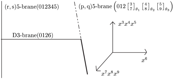
Figure 1: The brane configuration that we study below.

In the following, we will study how our $(r,s)$5-brane can be represented as a 5-brane in M-theory. For $(p,q)$5-brane, we can understand from the case of $(r,s)$5-brane by replacing $(r,s)$ with $(p,q)$ and $\{x^{k},x^{k+4}\}$ with $\{x^{k}\cos\theta_{k-2}+x^{k+4}\sin\theta_{k-2},x^{k+4}\cos\theta_{k-2}-x^{k}\sin\theta_{k-2}\}$ for $k=3,4,5$.

Let us consider an M5-brane whose world-volume is $(x^{0},x^{1},x^{2}\cos\phi_{\rm A}+x^{10}\sin\phi_{\rm A},x^{3},x^{4},x^{5})$. We can get the Type IIB 5-brane from this M5-brane by compactifying the two directions $x^{10}$-$x^{2}$ on a torus and taking T-duality [16]. We define the complex structure of this torus as

$$\tau=\frac{R_{2}\tan\alpha}{R_{10}}+i\frac{R_{2}}{R_{10}},$$ (1)

where ${R_{2}}$ and ${R_{10}}$ are the radii of the compactified $x_{2}$ and $x_{10}$, respectively, and $\alpha$ is the angle which represents the rotation between the direction of $x_{2}$ and the direction which has periodicity due to the compactification (see Fig. 2), denoted as ${x_{2}}^{\prime}$. If we shrink ${R_{10}}$ and take T-duality in the direction of ${x_{2}}^{\prime}$, we get Type IIB theory. In terms of the Type IIB string coupling constant $g_{s}\equiv\frac{R_{10}}{R_{2}}$ and the VEV $C_{0}\equiv\tan\alpha/g_{s}$ of RR 0-form, we can also write this complex structure as $\tau=C_{0}+\frac{i}{g_{s}}$.

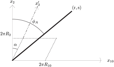
Figure 2: An M5-brane wrapping a torus $T^{2}$ $r$ times over $x_{10}$ and $s$ times over $x_{2}^{\prime}$.

On this torus, we can depict the Type IIB $(r,s)$5-brane as the M5-brane wrapping $x_{2}^{\prime}$ $s$ times and $x_{10}$ $r$ times. We thus set $\phi_{\rm A}$ as

$$\tan\phi_{\rm A}=\frac{rR_{10}+sR_{2}{\tan\alpha}}{sR_{2}}=\frac{r}{s}g_{s}+C_{0}g_{s}.$$ (2)

The corresponding angle $\phi_{B}$ for $(p,q)$5-brane is defined by replacing $(r,s)$ with $(p,q)$. As a result, our brane configuration can be expressed in M-theory as

$${\rm M5}\Big{[}01\left({2}\atop{10}\right)_{\phi_{A}}345\Big{]}-{\rm M2}\left(016\right)-{\rm M5}\Big{[}01\left({2}\atop{10}\right)_{\phi_{B}}\left({3}\atop{7}\right)_{\theta_{1}}\left({4}\atop{8}\right)_{\theta_{2}}\left({5}\atop{9}\right)_{\theta_{3}}\Big{]}$$

By analyzing the Killing spinors for the above three kinds of M-branes, the conditions for the unbroken SUSY have been obtained in [6] (see also [15], in which the authors study the unbroken SUSY of the two rotated M5-branes). The results are summarized as follows:

• $\frac{1}{16}$ ${\rm SUSY}$ ($3D$ $N=1$): $|\phi_{A}-\phi_{B}|=|\theta_{1}\pm\theta_{2}\pm\theta_{3}|$,

• $\frac{1}{8}$ ${\rm SUSY}$ ($3D$ $N=2$): $|\phi_{A}-\phi_{B}|=|\theta_{i}|$, $|\theta_{j}|=|\theta_{k}|$, $(i,j,k)=(1,2,3)$,

• $\frac{3}{16}$ ${\rm SUSY}$ ($3D$ $N=3$): $|\phi_{A}-\phi_{B}|=|\theta_{1}|=|\theta_{2}|=|\theta_{3}|$.

2.2 Mode expansions for vector fields

In this section, we will derive the mode expansions for the vector fields on the D3-brane from the boundary conditions which we derive now. Let us first consider the $4D$ field theory on the D3-brane whose world-volume is separated by NS5-brane or D5-brane. This is the case discussed in [2]. The action for the $4D$ gauge field with zero VEV of RR 0-form is given as

$$\int d^{3}xdx^{6}\left[-\frac{1}{4g_{YM_{4}}^{2}}F_{mn}F^{mn}\right],$$ (3)

where $d^{3}x\equiv dx^{0}dx^{1}dx^{2}$, $m$ and $n$ run over $0,1,2,6$, and $g_{YM_{4}}$ is the $4D$ gauge coupling constant in $4D$ $N=4$ SYM and is related to the string coupling constant by $g_{YM_{4}}^{2}=2\pi g_{s}$ [17].

Actually the theories are confined to the region $0\leq x^{6}\leq L$ by the two 5-branes. We are then left with surface terms from the boundaries of $x^{6}$ coordinate in making the variation of the action with respect to $A_{\mu}$. From the variation in the above action, we find the surface term

$$\int d^{3}x\delta A^{\mu}\frac{1}{g_{YM_{4}}^{2}}F_{\mu 6},$$ (4)

at the boundaries in the $x^{6}$ direction. These must vanish by themselves. Hanany and Witten suggest that the boundary condition is $F_{\mu\nu}=0$ ($\mu,\nu=0,1,2$) for D5-brane from the gauge invariant representation of $\delta A^{\mu}=0$ and $F_{\mu 6}=0$ for NS5-brane [2].

Now the question is what happens if there is non-zero VEV of RR 0-form in the above configuration. The action for the $4D$ gauge field with non-zero VEV of RR 0-form is given by

$$\int d^{3}xdx^{6}\Big{[}-\frac{1}{4g_{YM_{4}}^{2}}F_{mn}F^{mn}+\frac{C_{0}}{4\pi}\epsilon^{6\mu\nu\lambda}F_{6\mu}F_{\nu\lambda}\Big{]},$$ (5)

where $\mu,\nu$, and $\lambda$ run over $0,1,2$. From the variation of this action, by the same procedure as above, we are led to the boundary conditions

$$\frac{1}{g_{s}}F_{\mu 6}+C_{0}\frac{1}{2}\epsilon_{\mu\nu\lambda}F^{\nu\lambda} = 0\ \ \ {\rm for}\ \ {\rm NS5},$$ (6)

$$\frac{1}{2}\epsilon_{\mu\nu\lambda}F^{\nu\lambda} = 0\ \ \ {\rm for}\ \ {\rm D5}.$$ (7)

Note that the boundary condition on NS5-brane is changed and mixed with that of D5-brane, but the boundary condition on D5-brane is unchanged. In fact, for non-zero value of $C_{0}$, NS5-brane comes to have D5 charge by $C_{0}$ in addition to unit NS5 charge. This is expressed as $[C_{0},1]$ in the charge lattice, which can be seen Fig. 2 by counting the winding numbers in the directions of $x_{10}$ and $x_{2}$, and by using the relation, $C_{0}=\frac{R_{2}\tan\alpha}{R_{10}}$. This is a phenomenon similar to Witten effect in $4D$ field theory [18]. On the other hand, D5-brane has only one D5 charge, expressed as $[1,0]$, and its charge is not affected by non-zero $C_{0}$. So we expect that boundary condition for the 5-brane is given by mixing these two kinds of boundary conditions at the rate of the charges that the 5-brane has. For $(r,s)$5-brane with non zero $C_{0}$, the charge can be expressed as $[sC_{0}+r,s]$. We thus expect that the boundary condition can be obtained by replacing $C_{0}$ in (6) by $C_{0}+\frac{r}{s}$:

$$\frac{1}{g_{s}}F_{\mu 6}+(C_{0}+\frac{r}{s})\frac{1}{2}\epsilon_{\mu\nu\lambda}F^{\nu\lambda}=0.$$ (8)

This also includes the boundary condition for D5-brane, as can be seen by putting $(r,s)=(1,0)$. The term with the coefficient $\frac{r}{s}$ may be understood as coming from the condensation on the $(r,s)$5-brane just as the case of the fundamental string boundary condition on the bound state of D-branes. For $(p,q)$5-brane, we obtain the condition by replacing $(r,s)$ by $(p,q)$. Therefore in our model, we get the boundary conditions for the vector field as

$$F_{\mu 6}+(C_{0}+\frac{r}{s})g_{s}\frac{1}{2}\epsilon_{\mu\nu\lambda}F^{\nu\lambda}=0,\ \ \ {\rm at}\ \ \ x^{6}=0,$$

$$F_{\mu 6}+(C_{0}+\frac{p}{q})g_{s}\frac{1}{2}\epsilon_{\mu\nu\lambda}F^{\nu\lambda}=0,\ \ \ {\rm at}\ \ \ x^{6}=L.$$ (9)

Let us discuss the spectrum under these boundary conditions. Using (2) and

$$\tan\phi_{A}=(\frac{r}{s}+C_{0})g_{s},\hskip 14.22636pt\tan\phi_{B}=(\frac{p}{q}+C_{0})g_{s},$$ (10)

we can expand the $4D$ gauge fields as

$$A_{\mu} = \sum_{n=-\infty}^{\infty}a_{\mu}^{(n)}\cos[(\phi_{A}-\phi_{B}+n\pi)\frac{x_{6}}{L}-\phi_{A}],$$

$$A_{6} = \sum_{n=-\infty}^{\infty}a_{6}^{(n)}\sin[(\phi_{A}-\phi_{B}+n\pi)\frac{x_{6}}{L}-\phi_{A}],$$ (11)

up to gauge transformation. Here we denote by $a_{\mu}^{(n)}$ and $a_{6}^{(n)}$ the fields which depend on only $3D$ coordinates $x^{0},x^{1},x^{2}$. These expansions lead to the following representations for the $4D$ field strengths:

$$F_{\mu\nu} = \sum_{n=-\infty}^{\infty}f_{\mu\nu}^{(n)}\cos[(\phi_{A}-\phi_{B}+n\pi)\frac{x_{6}}{L}-\phi_{A}],$$

$$F_{\mu 6} = \sum_{n=-\infty}^{\infty}f_{\mu 6}^{(n)}\sin[(\phi_{A}-\phi_{B}+n\pi)\frac{x_{6}}{L}-\phi_{A}],$$ (12)

where $f_{\mu\nu}^{(n)}\equiv\partial_{\mu}a_{\nu}^{(n)}-\partial_{\nu}a_{\mu}^{(n)}$ and $f_{\mu 6}^{(n)}\equiv\partial_{\mu}a_{6}^{(n)}+\frac{(\phi_{A}-\phi_{B}+n\pi)}{L}a_{\mu}^{(n)}$. These mode expansions satisfy the boundary conditions (9) if we set

$$f_{\mu 6}^{(n)}=\frac{1}{2}\epsilon_{\mu\nu\lambda}f^{\nu\lambda(n)}.$$ (13)

In addition to the boundary conditions, these modes have to satisfy the equations of motion in $4D$ on the D3-brane. These equations can be expressed in terms of the corresponding modes as

$$\partial_{\mu}F^{\mu\nu}+\partial_{6}F^{6\nu} = 0\ \ \ \ \rightarrow\ \ \ \partial_{\mu}f^{\mu\nu(n)}-\frac{(\phi_{A}-\phi_{B}+n\pi)}{L}f^{\nu 6(n)}=0,$$ (14)

$$\partial_{\mu}F^{\mu 6} = 0\ \ \ \ \rightarrow\ \ \ \partial_{\mu}f^{\mu 6(n)}=0.$$ (15)

Obviously eq. (15) is satisfied due to eq. (13). For (14), we find

$$\partial_{\mu}f^{\mu\nu(n)} = \partial_{\mu}(-\epsilon^{\mu\nu\lambda}f_{\lambda 6}^{(n)})=-\epsilon^{\mu\nu\lambda}\partial_{\mu}\left[\partial_{\lambda}a_{6}^{(n)}+\frac{(\phi_{A}-\phi_{B}+n\pi)}{L}a_{\lambda}^{(n)}\right]$$ (16)

$$= -\frac{1}{2}\epsilon^{\mu\nu\lambda}\frac{(\phi_{A}-\phi_{B}+n\pi)}{L}f_{\mu\lambda}^{(n)}=\frac{(\phi_{A}-\phi_{B}+n\pi)}{L}\left(\frac{1}{2}\epsilon^{\nu\mu\lambda}f_{\mu\lambda}^{(n)}\right).$$

Thus eq. (14) is also satisfied by our modes. In fact the boundary conditions (9) and the field equations (14) and (15) are obeyed if and only if we impose the condition (13).

By eliminating $a_{6}^{(n)}$ from the condition (13) as in eq. (16), we get an equation for the $3D$ vector field $a_{\mu}^{(n)}$:

$$\partial_{\nu}f^{\nu\lambda(n)}-\frac{(\phi_{A}-\phi_{B}+n\pi)}{L}\frac{1}{2}\epsilon^{\mu\nu\lambda}f_{\mu\nu}^{(n)}=0.$$ (17)

The action in $3D$ which gives us eq. (17) as the field equation for $a_{\mu}^{(n)}$ is

$$\frac{L}{2\pi g_{s}}\int d^{3}x\Big{[}-\frac{1}{4}f_{\mu\nu}^{(n)}f^{\mu\nu(n)}-\frac{1}{4}\frac{(\phi_{A}-\phi_{B}+n\pi)}{L}\epsilon^{\mu\nu\lambda}a_{\lambda}^{(n)}f_{\mu\nu}^{(n)}\Big{]}.$$ (18)

This is the desired MCS action with the mass $\left|\frac{\phi_{A}-\phi_{B}+n\pi}{L}\right|$. To keep mass dimension one for the $3D$ gauge field, we have added the overall coefficient $\frac{L}{2\pi g_{s}}$, but in general, the overall factor can be absorbed in the definition of $a_{\mu}$.

From the condition (13), we can write the action in a form different from (18). Define

$$\frac{(\phi_{A}-\phi_{B}+n\pi)}{L}{\tilde{a}_{\mu}}^{(n)}\equiv\frac{(\phi_{A}-\phi_{B}+n\pi)}{L}a_{\mu}^{(n)}+\partial_{\mu}a_{6}^{(n)},$$ (19)

and we can rewrite (13) as

$$\frac{(\phi_{A}-\phi_{B}+n\pi)}{L}{\tilde{a}_{\mu}}^{(n)}=\frac{1}{2}\epsilon_{\mu\nu\lambda}{\tilde{f}^{\nu\lambda(n)}},$$ (20)

where ${\tilde{f}_{\mu\nu}^{(n)}}$ is the field strength for ${\tilde{a}_{\mu}}^{(n)}$. The action which gives us (20) as the equation of motion for ${\tilde{a}_{\mu}}^{(n)}$ is

$$\frac{L}{2\pi g_{s}}\int d^{3}x\Big{[}\frac{1}{4}\frac{(\phi_{A}-\phi_{B}+n\pi)}{L}\epsilon_{\mu\nu\lambda}{\tilde{a}^{\mu(n)}}{\tilde{f}^{\nu\lambda(n)}}-\frac{1}{2}\left(\frac{\phi_{A}-\phi_{B}+n\pi}{L}\right)^{2}{\tilde{a}_{\mu}}^{(n)}{\tilde{a}^{\mu(n)}}\Big{]}.$$ (21)

This is the action for self-dual model (SDM) with the mass $\left|\frac{\phi_{A}-\phi_{B}+n\pi}{L}\right|$. This shows that MCS theory and SDM are classically equivalent [19].

2.3 Comments on boundary conditions from supergravity solution

Let us examine the possibility to obtain the boundary condition for the vector field from the supergravity solution of the 5-brane. The classical solution for Type IIB $(r,s)$5-brane can be obtained from the solution of M5-brane following the procedure of [20]. The Type IIB $(r,s)$5-brane solution is

$${ds_{\rm IIB}}^{2} = H^{1/2}(\sin^{2}\phi_{\rm A}+H\cos^{2}\phi_{\rm A})^{1/2}\left[H^{-1}\left\{-(dx^{0})^{2}+(dx^{1})^{2}+(dx^{2})^{2}\right.\right.$$

$$\left.\left.+(dx^{3})^{2}+(dx^{4})^{2}+(dx^{5})^{2}\right\}+(dx^{6})^{2}+(dx^{7})^{2}+(dx^{8})^{2}+(dx^{9})^{2}\right],$$

$$\chi = \frac{R_{2}}{R_{10}\cos\alpha}\frac{\sin\phi_{\rm A}\cos(\phi_{\rm A}-\alpha)-H\sin(\phi_{\rm A}-\alpha)\cos\phi_{\rm A}}{\sin^{2}\phi_{\rm A}+H\cos^{2}\phi_{\rm A}},$$

$$e^{\phi} = \frac{R_{10}}{R_{2}}H^{-\frac{1}{2}}(\sin^{2}\phi_{\rm A}+H\cos^{2}\phi_{\rm A}),$$ (22)

$$H=1+\frac{Q(r,s)l_{s}^{2}}{R^{2}},\ \ \ \ Q(r,s)=g_{s}\sqrt{(r+C_{0}s)^{2}+\frac{s^{2}}{g_{s}^{2}}},$$

where $R$ is defined by $R^{2}=x_{6}^{2}+x_{7}^{2}+x_{8}^{2}+x_{9}^{2}$ and $l_{s}$ is the string length. Here we denote RR 0-form gauge field and dilaton by $\chi$ and $\phi$, respectively. Note that the asymptotic value of the axion $\chi$ is $C_{0}$, as it should be. Of course, there are backgrounds also for NSNS 2-form, RR 2-form and RR 4-form, but we will not need their explicit forms below. For $(p,q)$5-brane, we can get the solution from that of $(r,s)$5-brane by replacing $(r,s)$ with $(p,q)$ and $\{x^{k},x^{k+4}\}$ with $\{x^{k}\cos\theta_{k-2}+x^{k+4}\sin\theta_{k-2},x^{k+4}\cos\theta_{k-2}-x^{k}\sin\theta_{k-2}\}$ for $k=3,4,5$.

We can consider that the gravitational fields (graviton, dilaton, RR-gauge fields) are weakly coupled to the fields of $4D$ $N=4$ SYM theory. These gravity fields come from the $(p,q)$ and $(r,s)$5-branes on the ends of the D3-brane and we treat these as the external fields and approximate them by the classical SUGRA solution. We consider this system in the parameter region $g_{s}\ll 1$, $E\ll\frac{1}{l_{s}}$, where $E$ is the energy scale of the theory we are studying now, such as $3D$ SYM gauge coupling. This is the field theory limit, in which we can neglect the gravitational interactions and the corrections containing the powers of ${\alpha}^{\prime}$ and space-time is almost flat. Near 5-branes on both the ends of the D3-brane, where the distance from the 5-brane $R$ is much less than $l_{s}\sqrt{Q(r,s)}$, we have to take account of the gravitational effects as we can see from the form of the SUGRA solution. So when we make the variation of the $4D$ $N=4$ action weakly coupled to the gravity, it seems a good approximation to treat the equations of motion in the bulk as those in the flat background and derive the boundary conditions near each 5-brane in the limit $R\ll l_{s}\sqrt{Q(r,s)}$ of the SUGRA solution.

Let us consider the action for the gauge field coupled with gravity:

$$\int d^{3}xdx^{6}\Big{[}-\frac{\sqrt{-G}}{8\pi}{\rm e}^{-\phi}F_{mn}F^{mn}+\frac{\chi(x^{6})}{4\pi}\epsilon^{6\mu\nu\lambda}F_{6\mu}F_{\nu\lambda}\Big{]},$$ (23)

where $G=\prod_{i=0,1,2,6}G_{ii}$. Using the above supergravity solution, we see the coefficient of $F_{mn}F^{mn}$ reduces to the constant $-\frac{1}{8\pi g_{s}}$.

Since the theory is confined to the region $0\leq x^{6}\leq L$ by the two 5-branes, from the variation of the above action, we find the surface terms

$$\int d^{3}x\delta A^{\mu}\Big{[}\frac{1}{2\pi g_{s}}F_{\mu 6}+\frac{\chi(x^{6})}{2\pi}\frac{1}{2}\epsilon_{\mu\nu\lambda}F^{\nu\lambda}\Big{]},$$ (24)

at $x^{6}=0$ and $x^{6}=L$. These must vanish by themselves. We find that our boundary conditions are obtained by requiring that the square bracket in eq. (24) vanish at $x^{6}=0$ and $x^{6}=L$. Thus we get

$$\frac{1}{2\pi g_{s}}F_{\mu 6}+\frac{\chi(x^{6}=0)}{2\pi}\frac{1}{2}\epsilon_{\mu\nu\lambda}F^{\nu\lambda}=0,\ \ \ {\rm at}\ \ \ x^{6}=0,$$

$$\frac{1}{2\pi g_{s}}F_{\mu 6}+\frac{\chi(x^{6}=L)}{2\pi}\frac{1}{2}\epsilon_{\mu\nu\lambda}F^{\nu\lambda}=0,\ \ \ {\rm at}\ \ \ x^{6}=L.$$ (25)

By using the Type IIB solution for $\chi(x^{6})$, we can determine $\chi(x^{6})$ on the boundary as

$$\chi(x^{6}=0)\sim-\frac{R_{2}}{R_{10}\cos\alpha}\frac{\sin(\phi_{\rm A}-\alpha)\cos\phi_{\rm A}}{\cos^{2}\phi_{\rm A}}=C_{0}-\frac{{\rm tan}\phi_{\rm A}}{g_{s}}=-\frac{r}{s},$$ (26)

where use has been made of eq. (2).

Similarly we can get the condition at $x^{6}=L$ near $(p,q)$5-brane by replacing $(r,s)$ and $\phi_{\rm A}$ with $(p,q)$ and $\phi_{\rm B}$, respectively. Thus the boundary conditions in this approximation are

$$F_{\mu 6}-\frac{r}{s}g_{s}\frac{1}{2}\epsilon_{\mu\nu\lambda}F^{\nu\lambda}=0,\ \ \ {\rm at}\ \ \ x^{6}=0,$$

$$F_{\mu 6}-\frac{p}{q}g_{s}\frac{1}{2}\epsilon_{\mu\nu\lambda}F^{\nu\lambda}=0,\ \ \ {\rm at}\ \ \ x^{6}=L.$$ (27)

These conditions are different from those in (9). What is the reason for the difference and which are correct? In the present method using supergravity solutions, we have simply taken the $(r,s)$5-brane solution (22) and used its values at the boundaries. This is the so-called probe method. However, this neglects the contribution from the interaction between each 5-brane and the D3-brane at the end point of the D3-brane. Also there may be additional contributions from the difference between the equations of motion near the boundaries and in the bulk flat background. For these reasons, we believe that the derivation of the boundary conditions based on the 5-brane charges are more reliable. The boundary conditions in (9) also give $SL(2,{\bf Z})$-invariant spectrum, as we will discuss in section 4, and this gives another evidence that they are the correct ones.

2.4 Mode expansions for other fields

Next let us consider the scalar fields. The boundary conditions for those are the generalization of those in ref. [2]. It is argued that the scalar $\phi$ corresponding to the fluctuations in the direction along the 5-brane world-volume should have Neumann boundary condition $\partial_{6}\phi=0$ and those in the orthogonal directions Dirichlet condition $\partial_{\mu}\phi=0$. The conditions in our model at $x^{6}=0$ are thus

$$\partial_{6}X^{l}=0,$$

$$\partial_{\mu}X^{l+4}=0,\ \ {\rm at}\ \ x^{6}=0,$$ (28)

and those at $x^{6}=L$ are

$$\partial_{6}[X^{l}\cos\theta_{l-2}+X^{l+4}\sin\theta_{l-2}]=0,$$ (29)

$$\partial_{\mu}[-X^{l}\sin\theta_{l-2}+X^{l+4}\cos\theta_{l-2}]=0, {\rm at}\ \ x^{6}=L,$$

where $l=3,4,5$. For the above boundary conditions, we can make the mode expansions

$$X_{k+2}=\sum_{n=-\infty}^{\infty}\Phi_{k}^{(n)}\cos[(\theta_{k}+n\pi)\frac{x^{6}}{L}],$$

$$X_{k+6}=\sum_{n=-\infty}^{\infty}\Phi_{k}^{(n)}\sin[(\theta_{k}+n\pi)\frac{x^{6}}{L}],$$ (30)

where $k=1,2,3$, and $\{\Phi_{k}^{(n)}\}$ are the real scalar fields in $3D$ and depend only on $x^{0},x^{1},x^{2}$. Substituting these expressions into $X^{3},X^{4},X^{5},X^{7},X^{8},X^{9}$ in the original $4D$ action (see the appendix for the kinetic term of a complex scalar (two real scalars) in $4D$), we get

$$\frac{L}{2\pi g_{s}}\int d^{3}x\sum_{k=1}^{3}\sum_{n=-\infty}^{\infty}\left[-\frac{1}{2}\partial_{\mu}\Phi_{k}^{(n)}\partial^{\mu}\Phi_{k}^{(n)}-\frac{1}{2}\left(\frac{\theta_{k}+n\pi}{L}\right)^{2}{\Phi_{k}^{(n)}}^{2}\right].$$ (31)

This is the $3D$ massive scalar field theory with mass $\left|\frac{\theta_{k}+n\pi}{L}\right|$.

Finally let us discuss the fermions. There are four $4D$ Weyl fermions which have the origin in the $4D$ $N=4$ Abelian field theory on the D3-brane. These four fermions transform as spinor representation under $SO(6)$ R-transformation. Because of the relation $SO(6)\simeq SU(4)$, they transform as fundamental representation of $SU(4)$. The $4D$ four fermions in our model have the rotated boundary conditions which can be obtained by transforming those for the unrotated case.

For the unrotated case, we make the variation of the fermion kinetic terms with respect to each fermion and get

$${\bar{\lambda}}{\bar{\sigma}^{2}}\delta{\lambda}-\delta{\bar{\lambda}}{\bar{\sigma}^{2}}{\lambda}=0,$$ (32)

on the boundary, where ${\bar{\sigma}^{2}}=-\sigma^{2}$. Here $\sigma^{2}$ stands for the Pauli matrix in the $x^{6}$ direction. These conditions mean that ${\bar{\lambda}}=\pm\lambda$. If we decompose $\lambda$ as $\lambda=\sigma^{3}\frac{\lambda_{R}+i\lambda_{Im}}{\sqrt{2}}$, where $\lambda_{R}$ and $\lambda_{Im}$ are real spinors, we obtain the boundary condition $\lambda_{Im}=0$ for $+$ or $\lambda_{R}=0$ for $-$. We choose the boundary condition $\lambda_{Im}=0$ below.

In our model, we decompose the four $4D$ Weyl spinors $\lambda_{i}$ ($i=1,2,3,4$) into four pairs of real spinors as

$$\lambda_{l-2}=\frac{\sigma^{3}\left(\psi_{l}+i\psi_{l+4}\right)}{\sqrt{2}},\hskip 28.45274pt\lambda_{4}=\frac{\sigma^{3}\left(\psi_{2}+i\psi_{10}\right)}{\sqrt{2}},$$ (33)

where $l=3,4,5$. These combinations and indices are defined so as to correspond to the rotations of the 5-brane in the planes $x^{3}$-$x^{7}$, $x^{4}$-$x^{8}$ and $x^{5}$-$x^{9}$ by $\theta_{1}$, $\theta_{2}$ and $\theta_{3}$. Each $\lambda_{i}$ ($i=1,2,3,4$) transforms like $\lambda_{i}\to e^{-i\theta_{i}}\lambda_{i}$, where $\sum_{i=1}^{4}\theta_{i}=0$ from the traceless condition for $SU(4)$. Our above choice of the boundary conditions leads to ${\rm Im}\lambda_{i}=0$ at $x^{6}=0$ and ${\rm Im}{\left(e^{-i\theta_{i}}\lambda_{i}\right)}=0$ at $x^{6}=L$. We obtain

$$\psi_{7}=\psi_{8}=\psi_{9}=\psi_{10}=0,\ \ {\rm at}\ \ x^{6}=0,$$ (34)

and

$$-\psi_{l}\sin\theta_{l-2}+\psi_{l+4}\cos\theta_{l-2}=0,\ \ (l=3,4,5),$$

$$-\psi_{2}\sin\theta_{4}+\psi_{10}\cos\theta_{4}=0,\ \ {\rm at}\ \ x^{6}=L.$$ (35)

To satisfy these boundary conditions, we expand $4D$ real fermions in terms of $3D$ Majorana fermions as

$$\psi_{k+2}=\sum_{n=-\infty}^{\infty}\Psi_{k}^{(n)}\cos[(\theta_{k}+n\pi)\frac{x^{6}}{L}],\ \ \ \ \ \psi_{k+6}=\sum_{n=-\infty}^{\infty}\Psi_{k}^{(n)}\sin[(\theta_{k}+n\pi)\frac{x^{6}}{L}],$$

$$\psi_{2}=\sum_{n=-\infty}^{\infty}\Psi_{4}^{(n)}\cos[(\theta_{4}+n\pi)\frac{x^{6}}{L}],\ \ \ \ \ \psi_{10}=\sum_{n=-\infty}^{\infty}\Psi_{4}^{(n)}\sin[(\theta_{4}+n\pi)\frac{x^{6}}{L}],$$ (36)

where $\Psi_{k}^{(n)}$ ($k=1,\ldots,3$) and $\Psi_{4}^{(n)}$ are $3D$ Majorana spinors. Substituting these expressions into the original $4D$ SYM on the D3-brane, we get the $3D$ action

$$-\frac{1}{2\pi g_{s}}\int d^{3}xdx_{6}\sum_{i=1}^{4}\frac{i}{2}\Big{[}{\bar{\lambda}_{i}}{\bar{\sigma}^{\mu}}\partial_{\mu}{\lambda_{i}}-\partial_{\mu}{\bar{\lambda}_{i}}{\bar{\sigma}^{\mu}}{\lambda_{i}}+{\bar{\lambda}_{i}}{\bar{\sigma}^{2}}\partial_{6}{\lambda_{i}}-\partial_{6}{\bar{\lambda}_{i}}{\bar{\sigma}^{2}}{\lambda_{i}}\Big{]}$$

$$=\frac{L}{2\pi g_{s}}\int d^{3}x\sum_{k=1}^{4}\sum_{n=-\infty}^{\infty}\frac{i}{2}\Big{[}{\bar{\Psi}_{k}^{(n)}}\gamma^{\mu}\partial_{\mu}{\Psi_{k}^{(n)}}+\frac{\theta_{k}+n\pi}{L}{\bar{\Psi}_{k}^{(n)}}\Psi_{k}^{(n)}\Big{]},$$ (37)

where $\gamma^{\mu}$ is the $3D$ gamma matrices (see the appendix for their explicit forms and relation to Pauli matrices). This is the $3D$ action for massive Majorana fermions with the mass $\left|\frac{\theta_{k}+n\pi}{L}\right|$, ($k=1,\ldots,4$).

In summary, we have derived the $3D$ action containing vector fields, real scalar fields and Majorana fermions. They are all massive and have infinite sequences of higher modes.

Let us consider the theory in the limit that the higher modes decouple, in addition to taking the field theory limit, $g_{s}\ll 1$, $E\ll\frac{1}{l_{s}}$, where $E$ is the energy scale of the field theory we are studying now, such as the $3D$ SYM gauge coupling constant $g_{YM_{3}}^{2}=\frac{2\pi g_{s}}{L}$. Namely we consider our theory in the following parameter region:

$$E\ll\frac{1}{L}\ll\frac{1}{l_{s}}, g_{s}\ll 1,\ \ \ \ |\phi_{A}-\phi_{B}|\ll 1,\ \ \ \ |\theta_{k}|\ll 1;$$ (38)

$$\frac{g_{s}}{L},\ \ \frac{|\phi_{A}-\phi_{B}|}{L}\ \ {\rm and}\ \ \frac{|\theta_{k}|}{L}\ \ \ {\rm fixed},$$

where $k=1,\ldots,4$. Suppose that we integrate out all the higher modes with masses much larger than $E$ which is the energy scale of the field theory in our consideration. We are then left with a theory which consists of only $n=0$ modes:

$$\frac{L}{2\pi g_{s}}\int d^{3}x \Big{[}-\frac{1}{4}f_{\mu\nu}f^{\mu\nu}-\frac{1}{4}\frac{(\phi_{A}-\phi_{B})}{L}\epsilon^{\mu\nu\lambda}a_{\lambda}f_{\mu\nu}-\frac{1}{2}\sum_{k=1}^{3}\Big{(}\partial_{\mu}\Phi_{k}\partial^{\mu}\Phi_{k}+(\frac{\theta_{k}}{L})^{2}\Phi_{k}^{2}\Big{)}$$ (39)

$$+\frac{i}{2}\sum_{k=1}^{4}\Big{(}{\bar{\Psi}_{k}}\gamma^{\mu}\partial_{\mu}{\Psi_{k}}+\frac{\theta_{k}}{L}{\bar{\Psi}_{k}}\Psi_{k}\Big{)}\Big{]},$$

where the index $(n=0)$ on each field are suppressed. We call this limit the lowest mode limit in what follows.

3 Condition for supersymmetry

In this section, we discuss the number of unbroken SUSY in our theories described by the action (39). The conditions of the unbroken SUSY change according to the various relations among the masses. On the other hand, it is known from the analysis of the branes in M-theory which appear in our configuration that the four relative angles in the two M5-branes determine the unbroken SUSY in this configuration [15, 6]. We can compare these conditions for SUSY with those obtained from the analysis of the field theory on the D3-brane.

Let us study the theory (39) in the point of the SUSY. The combinations ($\Phi_{k}$,$\Psi_{k}$), ($k=1,2,3$) become $3D$ $N=1$ SUSY multiplets as we can see from the fact that they have the same mass $\left|\frac{\theta_{k}}{L}\right|$. But the gauge field has mass $\left|\frac{\phi_{A}-\phi_{B}}{L}\right|$ while the fourth fermion $\Psi_{4}$ has the mass $\left|\frac{\theta_{4}}{L}\right|$. These two masses are different in general, which means that there is no unbroken SUSY. If these two masses are the same, they constitute a $3D$ $N=1$ gauge multiplet and we have at least $3D$ $N=1$ SUSY. Thus the condition for $3D$ $N=1$ SUSY is

$$|\theta_{4}|=|\theta_{1}+\theta_{2}+\theta_{3}|=|\phi_{A}-\phi_{B}|.$$ (40)

Note that we can express $|\phi_{A}-\phi_{B}|$ in terms of $(r,s)$, $(p,q)$, $g_{s}$ and $C_{0}$ as

$$|{\tan}(\phi_{\rm A}-\phi_{\rm B})|=\left|\frac{qr-ps}{g_{s}(pr+sq|\tau|^{2})+C_{0}g_{s}(ps+qr)}\right|.$$ (41)

The condition for SUSY (40) is in agreement with the result in the M-theory summarized in subsection 2.1 for $3D$ $N=1$, that is, 1/16 SUSY in terms of the original $10D$ $N=2$ theory.

The discussions in refs. [15, 6] are based on the analysis of the system of two relatively rotated M5-branes and an M2-brane, in which they are treated as M-branes with infinite world-volumes. As a result, the contribution of the boundary of the M2-brane and of the intersections between M5-branes and M2-brane could be neglected. If we do not have such intersections in our configuration, the same SUSY is expected when we reduce the system with the two M5-branes and one M2-brane to that in IIA theory and convert it into the system in IIB theory by T-duality. The VEV of RR 0-form $C_{0}$ has no effects on the field theory on the D3-brane with infinite world-volume because the anomaly term $F\wedge F$ is a total derivative and topologically trivial in $4D$ Abelian theory. But if one direction of the D3-brane is finite by the existence of the intersections, this anomaly term does not vanish and might cause some discrepancy between the field theory and M-theory analyses. The above result shows that such discrepancy does not actually appear.

We can also derive the conditions for more SUSY from the relations among the masses of the four $3D$ $N=1$ multiplets. For example, if two of them and the rest are the same

$$|\theta_{1}|=\left|\phi_{A}-\phi_{B}\right|,\ \ \ \ \ |\theta_{2}|=|\theta_{3}|,$$ (42)

then we have $3D$ $N=2$ SUSY. In this case, we have one $N=2$ massive vector multiplet with mass $\frac{|\theta_{1}|}{L}$ and one $N=2$ massive hypermultiplet with mass $\frac{|\theta_{2}|}{L}$. This condition for 1/8 SUSY is again the same as the M-theory analysis in refs. [15, 6].

Moreover if all the four masses are the same

$$|\phi_{A}-\phi_{B}|=|\theta_{1}|=|\theta_{2}|=|\theta_{3}|,$$ (43)

we have $3D$ $N=3$ SUSY. $3D$ $N=3$ fields consist of one $N=2$ massive vector multiplet and one $N=2$ massive hypermultiplet with the same mass. Here also we reproduce the same result as that of [15, 6].

4 $SL(2,{\bf Z})$ transformation and spectrum

Let us discuss the invariance under the $SL(2,{\bf Z})$ transformation of the type IIB brane configuration. The boundary condition (9) for the gauge field has the T-invariance under

$$\left(\matrix{r\cr s\cr}\right)\to\left(\matrix{r-s\cr s\cr}\right),\ \ \ \ \left(\matrix{p\cr q\cr}\right)\to\left(\matrix{p-q\cr q\cr}\right),\ \ \ \ C_{0}\to C_{0}+1,$$ (44)

but the S-invariance under

$$\left(\matrix{r\cr s\cr}\right)\to\left(\matrix{s\cr-r\cr}\right),\ \ \ \ \left(\matrix{p\cr q\cr}\right)\to\left(\matrix{q\cr-p\cr}\right),\ \ \ \ \tau\to-\frac{1}{\tau},$$ (45)

is not so apparent. If there is any invariance of the spectrum under the $SL(2,{\bf Z})$ transformation, it would be the reflection of the $SL(2,{\bf Z})$ invariance in the $4D$ $N=4$ Abelian gauge theory realized on one D3-brane.

Let us consider the mass spectrum in our theory. The masses of the scalars and the fermions are invariant under the $SL(2,{\bf Z})$ transformation. It is the mass of the gauge field that may change under this transformation. We see that this mass is determined by the relative angle of the two M5-brane in the $x^{2}$-$x^{10}$ plane. The relative angle is $SL(2,{\bf Z})$ invariant, so we can conclude our spectrum are invariant under $SL(2,{\bf Z})$ transformation. In fact this can also be confirmed by direct calculation using the transformation

$$\left(\matrix{r\cr s\cr}\right)\rightarrow\left(\matrix{a&-b\cr-c&d\cr}\right)\left(\matrix{r\cr s\cr}\right),\ \ \ \ \left(\matrix{p\cr q\cr}\right)\rightarrow\left(\matrix{a&-b\cr-c&d\cr}\right)\left(\matrix{p\cr q\cr}\right),\ \ \ \ \tau\rightarrow\frac{a\tau+b}{c\tau+d},$$ (46)

where $a,b,c$ and $d$ are integers and satisfy $ad-bc=1$.

5 Comments on the theories with fundamental matters

We have considered the theories without matter until now. Here we study briefly how the theories with matters are changed, compared with those without matters. For simplicity, we set $C_{0}$ to zero below.

The matters in the (anti-)fundamental representation can be expressed by the open strings stretched between the D3-brane and D5-branes which have the world-volume ($x^{0},x^{1},x^{2},x^{7},x^{8},x^{9}$). So we need to add some D5-branes in addition to the configuration we have discussed. We consider the case with two D5-branes as a simple example. Moreover we will discuss below theories without mass terms for the (anti-)fundamentals and Fayet-Iliopoulos terms. We also put $(r,s)=(0,1)$, in which the condition for SUSY is the same as that without matter; D5-branes give no additional condition for the SUSY in the configuration we have discussed. The corresponding field theory is massive (MCS) Abelian gauge theory with two fundamental matters. The bosonic part of the action for the flavors [24, 25] is

$$S_{Q}=-\int d^{3}x\left[\sum_{\mu=0}^{2}\sum_{l=1}^{2}\left|(\partial_{\mu}+ia_{\mu})Q_{l}\right|^{2}+\sum_{l=1}^{2}Q^{{\dagger}}_{l}Q_{l}\sum_{k=1}^{3}\Phi_{k}^{2}\right.$$

$$\hskip 85.35826pt\left.+\frac{1}{2}\sum_{k=1}^{3}\left(g_{YM_{3}}\sum_{l=1}^{2}Q^{{\dagger}}_{l}\sigma^{k}Q_{l}+\frac{1}{g_{YM_{3}}}\frac{\theta_{k}}{L}\Phi_{k}\right)^{2}\right],\hskip 17.07164ptQ_{l}\equiv\left({q_{l}}\atop{{\tilde{q}_{l}}^{{\dagger}}}\right),$$ (47)

where $l$ is the index for the two flavors, and $q_{l}$ and $\tilde{q}_{l}$ are the fundamental and anti-fundamental matters, respectively. Here $g_{YM_{3}}$ is the 3D gauge coupling constant given by $g_{YM_{3}}^{2}=\frac{2\pi g_{s}}{L}$. The above action is the same as that for $3D$ $N=4$ charged hypermultiplets except the terms containing the angles.

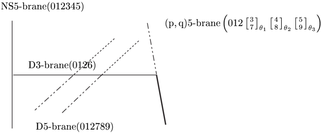
Figure 3: The brane configuration corresponding to the massive (CS) Abelian gauge theory with two fundamental matters.

Compared with ref. [2], there is no Coulomb branch (moduli) parameterized by the VEV of the adjoint fields, because they are all massive fields and cannot get VEV. In the brane configuration, this corresponds to the fact that the D3-brane cannot move in the directions of $x^{3,4,5}$. If the VEVs of the fundamental matters are zero, the gauge coupling goes to the strong coupling region in the low energy and this CS theory may become confining.

Another phase in this theory is the Higgs, in which the VEVs of the (anti-)fundamentals are non-zero and the gauge symmetry is broken. This vacuum is described by $\Phi_{k}=0$ and $\sum_{l=1}^{2}Q^{{\dagger}}_{l}\sigma^{k}Q_{l}=0$, where $k=1,2,3$. This phase can be expressed by the brane configuration in which the D3-brane is broken into three pieces separated by the two D5-branes and the second (middle) piece between the two D5-branes is away from the other two pieces along the directions $x^{7},x^{8}$ and $x^{9}$ of the world-volume of the D5-branes (see Figs. 3 and 4). This analysis is classical, so there may be quantum corrections.

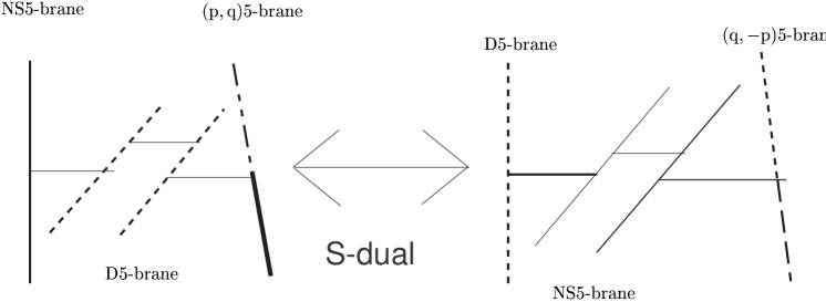
Figure 4: The classical brane configuration corresponding to the Higgs phase of the original theory and the Coulomb phase of the S-dual theory.

Let us discuss the S-transformation of this theory. By S-transformation, the above configuration changes into that in which NS5-brane, $(p,q)$5-brane and two D5-branes are replaced by D5-brane, $(q,-p)$5-brane and two NS5-branes, respectively. The field theory on this S-dual configuration is the Abelian gauge theory coming from the second (middle) D3-brane between the two NS5-branes. There are also two charged flavors with respect to this Abelian gauge symmetry. They originate from the open strings stretched between the second D3-brane and the first (left), and between the second D3-brane and the third (right). Their interaction terms take the same form as those in (47) with $\frac{\theta_{k}}{L}=0$, the same as the N=4 interaction terms. In addition, the matter field corresponding to the string stretched between the second D3-brane and the third is also charged with respect to the massive (MCS) Abelian gauge symmetry on the third (right) D3-brane. The massive Abelian fields are very heavy and their masses are ${\cal O}(\frac{1}{L})$ because we are considering the limit in which the rotation angles are close to $\frac{\pi}{2}$ (not $\phi_{A}-\phi_{B}$ and $\{\theta_{k}\}$) in this S-dual configuration. These large masses reduce $N=4$ to less SUSY and the heavy MCS fields couple to the charged matter in the same way as the interaction terms in (47) with large masses. The bosonic part of the action for the flavors in the S-dual theory is then

$$S_{B}=-\int d^{3}x\Bigg{[}\sum_{\mu=0}^{2}\sum_{l=1}^{2}\left|(\partial_{\mu}+i{\tilde{a}_{\mu}}-i\delta_{l2}c_{\mu})B_{l}\right|^{2}+\sum_{l=1}^{2}B^{{\dagger}}_{l}B_{l}\sum_{k=1}^{3}\left({\tilde{\Phi}_{k}}-\delta_{l2}\Theta_{k}\right)^{2}$$

$$+\frac{1}{2}\sum_{k=1}^{3}\left({\tilde{g}_{YM_{3}}^{(1)}}\sum_{l=1}^{2}B^{{\dagger}}_{l}\sigma^{k}B_{l}\right)^{2}+\frac{1}{2}\sum_{k=1}^{3}\left({\tilde{g}_{YM_{3}}^{(2)}}B^{{\dagger}}_{2}\sigma^{k}B_{2}+\frac{\kappa_{k}}{{\tilde{g}_{YM_{3}}^{(2)}}}\Theta_{k}\right)^{2}\Bigg{]},\;B_{l}\equiv\left({b_{l}}\atop{{\tilde{b}_{l}}^{{\dagger}}}\right),$$ (48)

where ${\tilde{g}_{YM_{3}}^{(1)}}$ and ${\tilde{g}_{YM_{3}}^{(2)}}$ are the $3D$ gauge coupling constants for the gauge theories on the second and third D3-branes. $B_{1}$ and $B_{2}$ are the matters corresponding to the open string stretching between the second D3-brane and the first, and the second D3-brane and the third. Their components $b_{l}$ and $\tilde{b}_{l}$ are the fundamental and anti-fundamental matters, respectively. Both the $B_{1}$ and $B_{2}$ couple to the $3D$ $N=4$ Abelian multiplet $({\tilde{a}_{\mu}},{\tilde{\Phi}_{k}})$. In addition to those, $B_{2}$ couples to the heavy MCS fields $(c_{\mu},\Theta_{k})$ on the third D3 with large masses.

In the lowest mode limit (38), these heavy CS fields should be integrated out. This yields

$$S_{B}=-\int d^{3}x\Bigg{[}\sum_{\mu=0}^{2}\sum_{l=1}^{2}\left|(\partial_{\mu}+i{\tilde{a}_{\mu}})B_{l}\right|^{2}+\sum_{l=1}^{2}B^{{\dagger}}_{l}B_{l}\sum_{k=1}^{3}{\tilde{\Phi}_{k}}^{2}$$

$$\hskip 128.0374pt+\frac{1}{2}\sum_{k=1}^{3}\left({\tilde{g}_{YM_{3}}^{(1)}}\sum_{l=1}^{2}B^{{\dagger}}_{l}\sigma^{k}B_{l}\right)^{2}+\sum_{k=1}^{3}{\cal O}\left(\frac{1}{\kappa_{k}}\right)\Bigg{]}.$$ (49)

The lowest mode limit (38) is nothing but the limit $\kappa_{k}\rightarrow\infty$ in the above. If we simply take the limit and ignore the interaction terms of ${\cal O}\left(\frac{1}{\kappa_{k}}\right)$, we get the same action as that for $3D$ $N=4$ SUSY. This appears to be inconsistent with the SUSY in the field theory realized on the original brane configuration. On the other hand, if we keep the terms of ${\tilde{a}_{\mu}}$, $B_{2}$ and ${\tilde{\Phi}_{k}}$ suppressed by the inverse of the large masses $\kappa_{k}$ after the integration, the SUSY would be the same as before the integration. Due to these two possibilities in the treatment of heavy modes, the Higgs branch is ambiguous as follows. If we keep the higher order terms, we can easily check that there is no Higgs branch because there is no vacuum with non-zero VEVs for the fundamentals and $\Theta_{k}={\tilde{\Phi}}=0$ in the action (48). This is consistent with the fact that the original field theory does not have the (would-be corresponding) Coulomb branch. If we simply ignore the higher order terms, the Higgs branch exists just as in ref. [2]. All of this suggests that we have to consider all the MCS higher modes without taking the lowest mode limit for the equivalence of the two theories related by the S-transformation. This is a complication that arises when we keep fields with non-zero masses.

Whatever the Higgs branch is, we can easily see that in this S-dual field theory, there is a Coulomb branch parameterized by non-zero ${\tilde{\Phi}_{k}}$ with $B_{l}=0$ and $\Theta_{k}=0$. This phase is expressed by the brane configuration in which the second D3-brane between the two NS5-branes is away from the other two pieces along the directions $x^{7},x^{8}$ and $x^{9}$ of the world-volume of the NS5-branes (see Fig.4).

We have classically studied the theory with fundamental matters and their S-dual theory. It is difficult to calculate the quantum corrections exactly, so we cannot say definitely whether these two theories are exactly equivalent in the low energy where the distances between the 5-branes do not appear. However, at least at the classical level, the Higgs branch of the original field theory seems to correspond to the Coulomb branch of its S-dual theory, as is seen from the brane configuration. If the two theories related by S-duality are the same theory in the low energy, probably all the MCS higher modes must be included.

6 Reduction to $2D$ and SUSY enhancement

In this section, we turn to the $2D$ theory which is obtained from (39) by dimensional reduction in the $x^{2}$ direction. This theory is realized on the D2-brane between two NS5-D4 bound states. This Type IIA configuration is related by T-duality to our Type IIB brane configuration that we have discussed.

Let us focus on the case $3D$ $N=3$ SUSY. We start with the action (39) under the condition (43). After adjusting the sign of the mass terms by changing the sign of the $3D$ Majorana fermion in the definition (33), we can write $3D$ $N=3$ action in the well-known form [21] (see the appendix for details)

$$\frac{L}{2\pi g_{s}}\int d^{3}x \Big{[}-\frac{1}{4}f_{\mu\nu}f^{\mu\nu}-\frac{\kappa}{4}\epsilon^{\mu\nu\lambda}a_{\lambda}f_{\mu\nu}-\frac{1}{2}\sum_{k=1}^{3}\Big{(}\partial_{\mu}\Phi_{k}\partial^{\mu}\Phi_{k}+\kappa^{2}\Phi_{k}^{2}\Big{)}$$ (50)

$$+\frac{i}{2}\sum_{k=2}^{4}\Big{(}{\bar{\Psi}_{k}}\gamma^{\mu}\partial_{\mu}{\Psi_{k}}-\kappa{\bar{\Psi}_{k}}\Psi_{k}\Big{)}+\frac{i}{2}\left({\bar{\Psi}_{1}}\gamma^{\mu}\partial_{\mu}{\Psi_{1}}+\kappa{\bar{\Psi}_{1}}\Psi_{1}\right)\Big{]},$$

where $\kappa$ is the CS mass. By the dimensional reduction in the $x^{2}$ direction, we obtain from (50)

$$\frac{L{\rm R}_{2}^{\prime}}{g_{s}}\int d^{2}x \Big{[}\ \frac{1}{2}f_{01}^{2}-\frac{1}{2}\partial_{\mu}\Phi_{4}\partial^{\mu}\Phi_{4}+\kappa f_{01}\Phi_{4}-\frac{1}{2}\sum_{k=1}^{3}\Big{(}\partial_{\mu}\Phi_{k}\partial^{\mu}\Phi_{k}+\kappa^{2}\Phi_{k}^{2}\Big{)}$$ (51)

$$+\frac{i}{2}\sum_{k=2}^{4}\Big{(}{\bar{\Psi}_{k}}\gamma^{\mu}\partial_{\mu}{\Psi_{k}}-\kappa{\bar{\Psi}_{k}}\Psi_{k}\Big{)}+\frac{i}{2}\left({\bar{\Psi}_{1}}\gamma^{\mu}\partial_{\mu}{\Psi_{1}}+\kappa{\bar{\Psi}_{1}}\Psi_{1}\right)\Big{]},$$

where $\Phi_{4}$ is the dimensionally reduced $3D$ gauge field $a_{2}$, and we denote the radius for the compactified direction by ${\rm R}_{2}^{\prime}\equiv\frac{R_{2}}{\cos\alpha}$ (see Fig. 2).

In the above action, the fermion masses break the $SO(4)$ invariance. However, we can eliminate $f_{01}$ since it is an auxiliary field and also make a chiral transformation ${\Psi_{1}}^{\prime}\equiv\gamma^{2}{\Psi_{1}}$ to obtain

$$\frac{L{\rm R}_{2}^{\prime}}{g_{s}}\int d^{2}x \Big{[}-\frac{1}{2}\sum_{k=1}^{4}\Big{(}\partial_{\mu}\Phi_{k}\partial^{\mu}\Phi_{k}+\kappa^{2}\Phi_{k}^{2}\Big{)}$$ (52)

$$+\frac{i}{2}\sum_{k=2}^{4}\Big{(}{\bar{\Psi}_{k}}\gamma^{\mu}\partial_{\mu}{\Psi_{k}}-\kappa{\bar{\Psi}_{k}}\Psi_{k}\Big{)}+\frac{i}{2}\left({\bar{\Psi}_{1}}^{\prime}\gamma^{\mu}\partial_{\mu}{\Psi_{1}}^{\prime}-\kappa{\bar{\Psi}_{1}}^{\prime}{{\Psi_{1}}^{\prime}}\right)\Big{]}.$$

This is the sigma model action with $2D$ (4,4) SUSY, that is, 1/4 SUSY compared with $10D$ $N=2$ theory. The SUSY is enhanced from 3/16 to 1/4 after dimensional reduction. It is crucial that as far as the degrees of freedom are concerned, there is no difference between $2D$ $N=(4,4)$ vector multiplet and $2D$ $N=(4,4)$ neutral hypermultiplet except that the vector multiplet has the gauge field without physical propagating modes; both of them consist of four real scalars and four fermions. The difference appears when the gauge interaction term exists. To keep these gauge interaction terms invariant under $2D$ $N=(4,4)$ transformation, the vector multiplet must be massless. So we cannot construct massive gauge theory with unbroken gauge symmetry in $2D$ $N=(4,4)$ theory. But in our case, the $3D$ $N=3$ massive vector multiplet reduces to $2D$ $N=(4,4)$ massive hypermultiplet. This happens only in Abelian gauge theory without charged matters. There is no gauge interaction in this theory. For non-Abelian gauge theory, $3D$ $N=3$ field theory reduces to $2D$ (3,3) non-Abelian gauge theory with some complicated interactions as well as the mass term for the gauge field. In the same way, the $3D$ $N=3$ MCS theory with fundamental matters reduces to $2D$ (3,3) field theory with fundamental matters. These two $N=3$ theories have gauge interactions, so the SUSY enhancement never occurs.

From the above calculations of the reduction from $3D$ to $2D$, we can say that this SUSY enhancement is accidental in $2D$ Abelian field theory due to the existence of the chiral transformation. This is the symmetry in $2D$ $N=(4,4)$ Abelian gauge theory, but not in $2D$ $N=(4,4)$ non-Abelian or $3D$ $N=4$ (massless) gauge theory (both for Abelian and non-Abelian). On the other hand, the $3D$ CS term breaks one of the four SUSY and is also not invariant under this kind of chiral transformation. When we reduce this term from $3D$ to $2D$, the broken SUSY transformation combined with the chiral transformation keeps the reduced CS term as well as $2D$ (4,4) Abelian action invariant. What we have found is that this transformation becomes the new SUSY transformation and SUSY is enhanced.

On the other hand, the SUSY of the brane configuration which realizes this $2D$ (4,4) massive theory is expected to be 3/16 [15, 6]. If we consider the gravity fields as well, we expect this kind of enhancement does not occur in this sector and the SUSY remains 3/16.

7 Conclusions and Discussions

We have discussed the spectrum of the theory on the D3-brane separated between $(r,s)$ and $(p,q)$5-branes. One of these 5-branes have rotated world-volumes with the three relative angles compared with the other. We regard this theory as the partially broken $4D$ $N=4$ theory by the boundary conditions. Assuming that the boundary conditions for the gauge field are determined by mixing the boundary conditions for the NS5-brane with vanishing VEV of RR 0-form gauge field and that for D5-brane at the rate of NS5 and D5 charges, we obtain the boundary conditions on the intersections of the D3-brane and $(r,s)$ or $(p,q)$5-branes. We also get the boundary conditions for the scalars and fermions by considering the direction of the rotated 5-brane world volume. We then find the modes which obey the boundary conditions as well as the equations of motion for the $4D$ Abelian fields on the D3-brane. From these modes we read off the $3D$ mass terms, which enable us to study the conditions for SUSY and the invariance under the Type IIB $SL(2,{\bf Z})$ transformation. We have found that the results for SUSY are the same as those in ref. [15, 6] in which the SUSY conditions are determined by the four relative angles of the rotated two M5-branes. We have also found that this theory has the $SL(2,{\bf Z})$ invariance. The masses we have obtained are determined by the $SL(2,{\bf Z})$-invariant relative angles of the two 5-branes, so the $SL(2,{\bf Z})$ invariance manifests itself even though the boundary conditions themselves are not manifestly invariant.

We have also discussed the case with matters by adding D5-branes. We can easily get its S-dual configuration, but identification of this S-dual field theory involves some ambiguity. The naive lowest mode limit in this theory is the $3D$ $N=4$ field theory, which appears to be in conflict with the the field theory with less SUSY of the original brane configuration. One possibility is that we have to include the contribution of the MCS higher modes without taking the lowest mode limit in order that these two theories are equivalent in the low energy where the distances between the 5-branes do not appear. That is, it is only in special cases such as $3D$ $N=4$ [2] that these two theories after taking the lowest mode limit are equivalent, and in general we need all the higher modes when we also include massive adjoint fields.

We have discussed only the case of one D3-brane, that is, Abelian theory. How about the non-Abelian theory? The boundary conditions are then non-linear, and it is difficult, if not impossible, to carry out the mode expansions as we have done for Abelian. As a result, it is premature to draw any definite conclusion about the non-Abelian theories. Intuitively, it seems that the field theory on the multiple D3-branes is $3D$ non-Abelian CS theory by the analogy with the Abelian theories. But there are the problems to be solved such as the quantization of the CS coefficient or the constraint of s-rule.

In ref. [6], it has been argued that for $C_{0}=0$ and $(r,s)=(0,1)$ in our model, there are Wilson lines whose VEVs are limited to the $p$ different values. This observation is based on the fact that in $T^{2}$ ($x^{2}$-$x^{10}$) compactified M-theory point of view, there are $p$ different positions on the M5-brane (corresponding to the $(p,q)$5-brane) to connect the other M5-brane (corresponding to (0,1)5-brane (NS5-brane)) by the M2-brane. These $p$ different positions in the compactified direction of $x^{2}$ correspond to the VEVs of the adjoint field $X_{2}$ in the IIA theory. This would require some potential terms for $X_{2}$ in the type IIA picture. After T-dual transformation, the VEVs of $X_{2}$ would turn into the Wilson lines in the type IIB theory. In ref. [6], it is suggested that the CS coefficient may explain the existence of these $p$ vacua. On the other hand, the field theoretic analysis in this paper is based on the boundary conditions derived by mixing those for D5- and NS5-branes at the rate of the charges and we believe that these conditions are the most natural ones from the field theory viewpoint. However, this analysis does not seem to indicate the existence of such Wilson lines and there is no indication of the potential in T-dualized theory within our IIB boundary conditions. It shows that there are many $3D$ CS gauge fields with heavy CS mass terms (large CS coefficient). It seems difficult to connect the CS coefficient to the $p$ vacua without taking this into account. There is a single vacuum in our 3D MCS theory, but this fact seems to be in contradiction to the above $p$ vacua originated from M-theory. It is possible that the information about $p$ different vacua might be dropped in the process from M-theory to Type IIB theory. If we can find boundary conditions which reflect such information coming from M-theory, we might construct 3D field theory that has these $p$ different vacua. That will be a complicated theory. How to determine this theory is an interesting subject left for future study.

Appendix

In this appendix, we will explain our notations in this paper and the method of the dimensional reduction. We show how to obtain $3D$ $N=4$ action by dimensional reduction from $4D$ $N=2$ SYM as an example. We also exhibit the $4D$ $N=2$ and $3D$ $N=4$ SUSY transformation, some of which remain unbroken in our model. Our notations in $4D$ SYM are those of [27] in which $4D$ $N=1$ is discussed in detail in the superspace formalism. We discuss $SU(N_{c})$ gauge theory, the Abelian case being straightforward.

The action of the $4D$ $N=2$ SYM is

$$\int d^{4}x{\cal L}_{4D}=\int d^{4}x\left[\frac{1}{2}{\rm Tr}(W^{\alpha}W_{\alpha}|_{\theta\theta}+\bar{W}_{\dot{\alpha}}\bar{W}^{\dot{\alpha}}|_{{\bar{\theta}}{\bar{\theta}}})+2{\rm Tr}\Phi^{\dagger}e^{2V}\Phi|_{\theta\theta{\bar{\theta}}{\bar{\theta}}}\right]$$

$$=\int d^{4}x\Big{[}-\frac{1}{4}F_{mn}^{(a)}F^{mn(a)}-\frac{i}{2}\sum_{k=1,2}\Big{(}\bar{\lambda}_{k}^{(a)}\bar{\sigma}^{m}D_{m}\lambda_{k}^{(a)}-D_{m}{\bar{\lambda}_{k}^{(a)}}\bar{\sigma}^{m}\lambda_{k}^{(a)}\Big{)}-D_{m}\phi^{a}D^{m}\phi^{a{\dagger}}$$

$$\hskip 56.9055pt+\frac{1}{2}D_{a}^{2}+|F^{a}|^{2}+\sqrt{2}(\phi^{{\dagger}}_{b}\lambda_{2c}\lambda_{1a}t_{acb}-\phi_{b}\bar{\lambda}_{1a}\bar{\lambda}_{2c}t_{abc})+it_{acb}D^{a}\phi_{c}\phi^{{\dagger}}_{b}\Big{]},$$ (53)

where $W^{\alpha}$ ($V$) and $\Phi$ are the $N=1$ superfields for the vector multiplet $(A_{m}^{a},\lambda_{1\alpha}^{a},D^{a})$, and the adjoint chiral multiplet, $(\phi^{a},\lambda_{2}^{a},F^{a})$. We take the Wess-Zumino gauge and drop the unphysical fields. The signature is $(-1,+1,+1,+1)$. The index for $4D$ Weyl spinor is $\alpha$ ($\alpha=1,2$), while $a$ ($a=1,\ldots,N_{c}^{2}-1$) is that for the non-Abelian gauge group generators $T^{a}$ in the fundamental representation. These generators satisfy $[T^{a},T^{b}]=it_{abc}T^{c}$ and ${\rm Tr}T^{a}T^{b}=\frac{\delta^{ab}}{2}$. The covariant derivatives and the field strengths are

$$D_{m}\phi^{a}\equiv\partial_{m}\phi^{a}-t_{abc}A^{b}_{m}\phi^{c},$$

$$F_{mn}^{(a)}\equiv\partial_{m}A_{n}^{a}-\partial_{n}A_{m}^{a}-t_{abc}A^{b}_{m}A^{c}_{n}.$$ (54)

The SUSY transformations for the above theory are

$$\delta A_{m}^{a}=-i{\bar{\lambda}_{1}}^{a}{\bar{\sigma}_{m}}\xi_{2}+i{\bar{\xi}_{2}}{\bar{\sigma}_{m}}\lambda_{1}^{a}+i{\bar{\lambda}_{2}}^{a}{\bar{\sigma}_{m}}\xi_{1}-i{\bar{\xi}_{1}}{\bar{\sigma}_{m}}\lambda_{2}^{a},$$

$$\delta\phi^{a}=\sqrt{2}(\xi_{1}\lambda_{1}^{a}+\xi_{2}\lambda_{2}^{a}),$$

$$\delta\lambda_{1}^{a}=\sigma^{mn}\xi_{2}F_{mn}^{a}+i\xi_{2}D^{a}+i\sqrt{2}\sigma^{m}\bar{\xi}_{1}D_{m}\phi^{a}+\sqrt{2}\xi_{1}F^{a*},$$

$$\delta\lambda_{2}^{a}=-\sigma^{mn}\xi_{1}F_{mn}^{a}+i\xi_{1}D^{a}+i\sqrt{2}\sigma^{m}\bar{\xi}_{2}D_{m}\phi^{a}+\sqrt{2}\xi_{2}F^{a},$$

$$\delta F^{a}=i\sqrt{2}\bar{\xi}_{2}\bar{\sigma}^{m}D_{m}\lambda_{2}^{a}-2t_{abc}\phi^{c}\bar{\xi}_{2}\bar{\lambda}_{1}^{b}+\left(i\sqrt{2}\bar{\xi}_{1}\bar{\sigma}^{m}D_{m}\lambda_{1}^{a}+2t_{abc}\phi^{c}\bar{\xi}_{1}\bar{\lambda}_{2}^{b}\right)^{\ast},$$

$$\delta D^{a}=-\xi_{2}\sigma^{m}D_{m}\bar{\lambda}_{1}^{a}-D_{m}\lambda_{1}^{a}\sigma^{m}\bar{\xi}_{2}+\xi_{1}\sigma^{m}D_{m}\bar{\lambda}_{2}^{a}+D_{m}\lambda_{2}^{a}\sigma^{m}\bar{\xi}_{1}$$

$$\hskip 56.9055pt+2it_{abc}\sqrt{2}(\xi_{1}\lambda_{1}^{c}\phi^{b*}-\phi^{b}\bar{\lambda}_{1}^{c}\bar{\xi}_{1}).$$ (55)

Let us consider the theory dimensionally reduced to $3D$ $N=4$ from the above $4D$ $N=2$ Lagrangian. The signature of our metric is $(-1,+1,+1)$ in $3D$ as in $4D$ and $\epsilon_{012}=-\epsilon^{012}=+1$. We take $x^{2}$ as the direction of dimensional reduction. After reduction, we rename the $x^{3}$ direction the new $x^{2}$. The fields of $4D$ $N=2$ SYM reduce to $3D$ $N=4$ as

$$A_{2}^{a}=C_{1}^{a},\ \ \ \ \ \ \phi^{a}=\frac{-C_{2}^{a}+iC_{3}^{a}}{\sqrt{2}},$$

$$F^{a}=\frac{-D_{3}^{a}+iD_{2}^{a}}{\sqrt{2}},\ \ \ \ D^{a}=-D_{1}^{a}+t_{abc}C_{2}^{b}C_{3}^{c},$$

$$\lambda_{k\alpha}^{a}=\frac{\sigma^{3}(\psi_{2k\alpha}^{a}+i\psi_{2k-1\alpha}^{a})}{\sqrt{2}},\ \ \ \ \ \bar{\lambda}_{k\dot{\alpha}}^{a}=\frac{\sigma^{3}(\psi_{2k\alpha}^{a}-i\psi_{2k-1\alpha}^{a})}{\sqrt{2}},\ \ \ (k=1,2).$$ (56)

We define $\{\lambda_{2},\lambda_{3},\lambda_{1},-\chi\}\equiv\{\psi_{1},\psi_{2},\psi_{3},\psi_{4}\}$, and the $3D$ gamma matrices by $\{\gamma^{\mu}\equiv\sigma^{3}(i\sigma^{2})\bar{\sigma}^{m}\sigma^{3}\}=(i\sigma^{2},-\sigma^{3},-\sigma^{1})$, where $\mu=0,1,2$ and $m=0,1,3$. We also define $\bar{\psi}_{\alpha}$ by $\bar{\psi}_{\alpha}\equiv\psi_{\beta}(-i\sigma^{2})_{\beta\alpha}$ and we always keep down the indices of spinor.

The $3D$ $N=4$ Lagrangian in these notations is

$${\cal L}_{3D} = -\frac{1}{4}F_{\mu\nu}^{(a)}F^{\mu\nu(a)}+\frac{i}{2}\sum_{k=1}^{3}\bar{\lambda}_{k}^{(a)}\gamma^{\mu}D_{\mu}\lambda_{k}^{(a)}+\frac{i}{2}\bar{\chi}^{(a)}\gamma^{\mu}D_{\mu}\chi^{(a)}$$ (57)

$$+ \frac{1}{2}\sum_{k=1}^{3}\left(-D_{\mu}C^{a}_{k}D^{\mu}C^{a}_{k}+D_{k}^{a2}\right)+\frac{it_{abc}}{2}\left(-\epsilon^{ijk}{\bar{\lambda}_{i}^{a}}\lambda_{j}^{b}C_{k}^{c}+2\sum_{k=1}^{3}{\bar{\lambda}_{k}^{a}}\chi^{b}C_{k}^{c}\right)$$

$$\hskip 56.9055pt-\frac{1}{4}\sum_{i,j=1}^{3}(C_{i}^{a}C_{j}^{b}t_{abc})^{2},$$

where $\epsilon^{ijk}$ is anti-symmetric tensor and $\epsilon^{123}=1$. The SUSY transformation follows from that of $4D$:

$$\delta A_{\mu}^{a} = i\sum_{k=1}^{3}\bar{\eta}_{k}\gamma_{\mu}\lambda_{k}^{a}+i\bar{\eta_{0}}\gamma_{\mu}\chi^{a},$$

$$\delta\lambda_{k}^{a} = \frac{i}{2}\gamma^{\mu}F^{\nu\rho(a)}\epsilon_{\mu\nu\rho}\eta_{k}-\epsilon_{kij}(D_{i}^{a}\eta_{j}-\gamma^{\mu}D_{\mu}C_{i}^{a}\eta_{j})-t_{abc}C_{k}^{b}\sum_{i\neq k}C_{i}^{c}\eta_{i}$$

$$+\frac{1}{2}t_{abc}\epsilon_{kij}C_{i}^{b}C_{j}^{c}\eta_{0}+\gamma^{\mu}D_{\mu}C_{k}^{a}\eta_{0}+\eta_{0}D_{k}^{a},$$

$$\delta\chi^{a} = -\gamma^{\mu}D_{\mu}\sum_{k=1}^{3}C_{k}^{a}\eta_{k}-\frac{1}{2}t_{abc}\epsilon_{kij}C_{j}^{b}C_{k}^{c}\eta_{i}-\sum_{k=1}^{3}\eta_{k}D_{k}^{a}+\frac{1}{2}\gamma^{\mu}F^{\nu\rho(a)}\epsilon_{\mu\nu\rho}\eta_{0},$$

$$\delta C_{k}^{a} = -i\epsilon_{ijk}\bar{\eta_{i}}\lambda_{j}^{a}+i\bar{\eta}_{k}\chi^{a}-i\bar{\eta}_{0}\lambda_{k}^{a},$$

$$\delta D_{k}^{a} = i\epsilon_{ijk}\bar{\eta}_{i}\gamma^{\mu}D_{\mu}\lambda_{j}^{a}+i\bar{\eta}_{k}\gamma^{\mu}D_{\mu}\chi^{a}+it_{abc}\left(\epsilon_{ijk}\bar{\eta}_{i}\chi^{b}C_{j}^{c}-\sum_{i=1}^{3}\bar{\eta}_{i}\lambda_{k}^{b}C_{i}^{c}\right)$$ (58)

$$+it_{abc}\left(\sum_{i=1}^{3}\bar{\eta}_{i}\lambda_{i}^{b}C_{k}^{c}-\sum_{i=1}^{3}\bar{\eta}_{k}\lambda_{i}^{b}C_{i}^{c}\right)-i\bar{\eta}_{0}\gamma^{\mu}D_{\mu}\lambda_{k}^{a}+it_{abc}\bar{\eta}_{0}(\epsilon_{ijk}\lambda_{i}^{b}C_{j}^{c}-\chi^{b}C_{k}^{c}),$$

If we add CS term

$${\cal L}_{CS}= \kappa\Big{[}-\frac{1}{2}\epsilon^{\mu\nu\rho}(A_{\mu}^{a}\partial_{\nu}A_{\rho}^{a}-{t_{abc}\over 3}A_{\mu}^{a}A_{\nu}^{b}A_{\rho}^{c})-\frac{i}{2}\left(\sum_{k=1}^{3}\bar{\lambda}_{k}^{a}\lambda_{k}^{a}-\bar{\chi^{a}}\chi^{a}\right)$$ (59)

$$\hskip 28.45274pt+\sum_{k=1}^{3}C_{k}^{a}D_{k}^{a}-{1\over 6}t_{abc}\epsilon_{ijk}C_{i}^{a}C_{j}^{b}C_{k}^{c}\Big{]},$$

we have $3D$ $N=3$ SUSY [21]. Only three of the above $3D$ $N=4$ SUSYs survive if we add this CS term. The transformation by $\eta_{0}$ is broken by this CS term. In the Abelian case, we can get the theory with less SUSY if we change the masses for $3D$ $N=1$ multiplets, $(A_{\mu},\lambda_{1})$, $(C_{1},\chi)$, $(C_{2},\lambda_{3})$ and $(C_{3},\lambda_{2})$.

Finally let us make the dimensional reduction of the $3D$ $N=3$ MCS theory to the $2D$ massive one in the $x^{2}$ direction. We obtain for this $2D$ theory

$${\cal L}_{2D+CS}= \frac{1}{2}\sum_{k=1}^{4}\left(i\bar{\lambda}_{k}^{(a)}\gamma^{\mu}\partial_{\mu}\lambda_{k}^{(a)}-\partial_{\mu}C^{a}_{k}\partial^{\mu}C^{a}_{k}+D_{k}^{a2}\right)$$ (60)

$$\hskip 56.9055pt+\kappa\left(\sum_{k=1}^{4}C_{k}^{a}D_{k}^{a}-\sum_{i=1}^{3}\frac{i}{2}\bar{\lambda}_{i}^{a}\lambda_{i}^{a}+\frac{i}{2}\bar{\lambda_{4}^{a}}\lambda_{4}^{a}\right),$$

where $D_{4}\equiv F_{01}$, $C_{4}\equiv A_{2}$ and $\lambda_{4}\equiv\chi$ and $\mu$ runs over $0$ and $1$. Of course, this is invariant under the original $2D$ (3,3) SUSY transformations. After we replace $\lambda_{k}$ $(k=1,\ldots,4)$ by $\gamma^{2}\lambda_{k}$ in the $\eta_{0}$ transformation reduced from $3D$ to $2D$, we get

$$\delta C_{i}^{a}=i\left(\overline{\gamma^{2}\eta_{0}}\right)\lambda_{i}^{a},\ \ \ \delta\lambda_{i}^{a}=\left[D_{i}^{a}-\gamma^{\mu}\partial_{\mu}C_{i}\right]\left(\gamma^{2}\eta_{0}\right),\ \ \ \delta D_{i}^{a}=-i\left(\overline{\gamma^{2}\eta_{0}}\right)\gamma^{\mu}\partial_{\mu}\lambda_{i}^{a},$$

$$\delta C_{4}^{a}=i\bar{\eta_{0}}\lambda_{i}^{a},\ \ \ \delta\lambda_{4}^{a}=-\left[D_{4}^{a}+\gamma^{\mu}\partial_{\mu}C_{4}\right]\eta_{0},\ \ \ \delta D_{4}^{a}=i\bar{\eta_{0}}\gamma^{\mu}\partial_{\mu}\lambda_{4}^{a},$$ (61)

where $i=1,2,3$. Under this transformation, we find that the $2D$ massive Lagrangian (60) is invariant. This is the new SUSY transformation besides the original $2D$ (3,3) SUSY and the $2D$ massive theory described by (60) has $2D$ (4,4) SUSY.

References

• [1] K. Intriligator and N. Seiberg, Phys.ย Lett.ย B387 (1996) 513, hep-th/9607207.
• [2] A. Hanany and E. Witten, Nucl.ย Phys.ย B492 (1997) 152, hep-th/9611230.
• [3] M. Porrati and A. Zaffaroni, Nucl.ย Phys.ย B490 (1997) 107, hep-th/9611201.
• [4] J. de Boer, K. Hori, H. Ooguri, Y. Oz and Z. Yin, Nucl.ย Phys.ย B493 (1997) 148, hep-th/9612131.
• [5] J. de Boer, K. Hori, Y. Oz and Z. Yin, Nucl.ย Phys.ย B502 (1997) 107, hep-th/9702154.
• [6] T. Kitao, K. Ohta and N. Ohta, Nucl.ย Phys.ย B539 (1999) 79, hep-th/9808111.
• [7] M.Gremm and E. Katz, hep-th/9906020.
• [8] J. de Boer, K. Hori, Y. Oz and Z. Yin, Nucl.ย Phys.ย B500 (1997) 163, hep-th/9703100.
• [9] O. Aharony, A. Hanany, K. Intriligator, N. Seiberg and M. J. Strassler, Nucl.ย Phys.ย B499 (1997) 67, hep-th/9703110.
• [10] A. Karch, Phys.ย Lett.ย B405 (1997) 79, hep-th/9703172.
• [11] O. Aharony, Phys.ย Lett.ย B404 (1997) 71, hep-th/9703215.
• [12] A. Kapustin and M. J. Strassler, JHEPย 9904 (1999) 021, hep-th/9902033.
• [13] J.P. Gauntlett, G.W. Gibbons, G. Papadopoulos and P.K. Townsend, Nucl.ย Phys.ย B500 (1997) 133, hep-th/9702202.
• [14] N. Ohta and J.-G. Zhou, Phys.ย Lett.ย B418 (1998) 70, hep-th/9709065.
• [15] N. Ohta and P.K. Townsend, Phys.ย Lett.ย B418 (1998) 77, hep-th/9710129.
• [16] J.H. Schwarz, Phys.ย Lett.ย B360 (1995) 13, hep-th/9508143.
• [17] N. Itzhaki, J.M. Maldacena, J. Sonnenschein and S. Yankielowicz, Phys.ย Rev.ย D58 (1998) 046004, hep-th/9802042.
• [18] E. Witten, Phys.ย Lett.ย B86 (1979) 283.
• [19] S. Deser and R. Jackiw, Phys.ย Lett.ย 139B (1984) 371.
• [20] E. Bergshoeff, C.M. Hull and T. Ortรญn, Nucl.ย Phys.ย B451 (1995) 547, hep-th/9504081.
• [21] H.-C. Kao, K. Lee and T. Lee, Phys.ย Lett.ย B373 (1996) 94, hep-th/9506170.
• [22] K. Ohta, JHEPย 9906 (1999) 025, hep-th/9904118.
• [23] B.-H. Lee, H.-j. Lee, N. Ohta, and H.-S. Yang, Phys.ย Rev.ย D60 (1999) 106003, hep-th/9904181.
• [24] J. Polchinski, โ€™TASI lectures on D-branesโ€™, hep-th/9611050.
• [25] H.-C. Kao, Phys.ย Rev.ย D50 (1994) 2881.
• [26] I. Ichinose and M. Onoda, Nucl.ย Phys.ย B435 (1995) 637.
• [27] J. Wess and J. Bagger, โ€˜Supersymmetry and Supergravityโ€™, Princeton University Press.