hep-th/9907219

July 1999

SISSA/113/99/FM, CERN-TH/99-231

3D superconformal theories
from Sasakian seven-manifolds:

new nontrivial evidences for $AdS_{4}/CFT_{3}$ ^∗
Davide Fabbri¹, Pietro Fré¹, Leonardo Gualtieri¹, Cesare Reina²,

Alessandro Tomasiello², Alberto Zaffaroni³ and Alessandro Zampa²

¹ Dipartimento di Fisica Teorica, Universitá di Torino, via P. Giuria 1, I-10125 Torino,
Istituto Nazionale di Fisica Nucleare (INFN) - Sezione di Torino, Italy
² International School for Advanced Studies (ISAS), via Beirut 2-4, I-34100 Trieste
³ CERN, Theoretical Division, CH 1211 Geneva, Switzerland,

In this paper we discuss candidate superconformal ${\cal N}=2$ gauge theories that realize the AdS/CFT correspondence with M–theory compactified on the homogeneous Sasakian $7$-manifolds $M^{7}$ that were classified long ago. In particular we focus on the two cases $M^{7}=Q^{1,1,1}$ and $M^{7}=M^{1,1,1}$, for the latter the Kaluza Klein spectrum being completely known. We show how the toric description of $M^{7}$ suggests the gauge group and the supersingleton fields. The conformal dimensions of the latter can be independently calculated by comparison with the mass of baryonic operators that correspond to $5$–branes wrapped on supersymmetric $5$–cycles and are charged with respect to the Betti multiplets. The entire Kaluza Klein spectrum of short multiplets agrees with these dimensions. Furthermore, the metric cone over the Sasakian manifold is a conifold algebraically embedded in some ${\mathbb{C}}^{p}$. The ring of chiral primary fields is defined as the coordinate ring of ${\mathbb{C}}^{p}$ modded by the ideal generated by the embedding equations; this ideal has a nice characterization by means of representation theory. The entire Kaluza Klein spectrum is explained in terms of these vanishing relations. We give the superfield interpretation of all short multiplets and we point out the existence of many long multiplets with rational protected dimensions, whose presence and pattern were already noticed in other compactifications and seem to be universal.

 ^∗ Supported in part by EEC under TMR contract ERBFMRX-CT96-0045 and by GNFM.

1 Synopsis

In this paper we consider M–theory compactified on anti de Sitter four dimensional space $AdS_{4}$ times a homogeneous Sasakian $7$–manifold $M^{7}$ and we study the correspondence with the infrared conformal point of suitable $D=3,{\cal N}=2$ gauge theories describing the appropriate M2–brane dynamics. For the reader’s convenience we have divided our paper into three parts.

• Part I contains a general discussion of the problem we have addressed and a summary of all our results.

• Part II presents the superconformal gauge–theory interpretation of the Kaluza Klein multiplet spectra previously obtained from harmonic analysis and illustrates the non–trivial predictions one obtains from such a comparison.

• Part III provides a detailed analysis of the algebraic geometry, topology and metric structures of homogeneous Sasakian $7$–manifolds. This part contains all the geometrical background and the explicit derivations on which our results and conclusions are based.

Part I General Discussion

2 Introduction

The basic principle of the AdS/CFT correspondence [1, 2, 3] states that every consistent M-theory or type II background with metric $AdS_{p+2}\times M^{d-p-2}$ in d-dimensions, where $M^{d-p-2}$ is an Einstein manifold, is associated with a conformal quantum field theory living on the boundary of $AdS_{p+2}$. The background is typically generated by the near horizon geometry of a set of p-branes and the boundary conformal field theory is identified with the IR limit of the gauge theory living on the world-volume of the p-branes. One remarkable example with ${\cal N}=1$ supersymmetry on the boundary and with a non-trivial smooth manifold $M^{5}=T^{1,1}$ was found in [4] and the associated superconformal theory was identified. Some general properties and the complete spectrum of the $T^{1,1}$ compactification have been discussed in [5, 6, 7], finding complete agreement between gauge theory expectations and supergravity predictions. In this paper we will focus on the case $p=2$ when $M$ is a coset manifold $G/H$ with ${\cal N}=2$ supersymmetry.

Backgrounds of the form $AdS_{4}\times M^{7}$ arise as the near horizon geometry of a collection of M2-branes in M-theory. The ${\cal N}=8$ supersymmetric case corresponds to $M^{7}=S^{7}$. Examples of superconformal theories with less supersymmetry can be obtained by orbifolding the M2-brane solution [8, 9]. Orbifold models have the advantage that the gauge theory can be directly obtained as a quotient of the ${\cal N}=8$ theory using standard techniques [10]. On the other hand, the internal manifold $M^{7}$ is $S^{7}$ divided by some discrete group and it is generically singular. Smooth manifolds $M^{7}$ can be obtained by considering M2-branes sitting at the singular point of the cone over $M^{7}$, ${\cal C}(M^{7})$ [4, 11, 12]. Many examples where $M^{7}$ is a coset manifold $G/H$ were studied in the old days of KK theories [13] (see [14, 15, 16, 17, 18, 19, 20, 21, 22] for the cases $S^{7}$ and squashed $S^{7}$, see [23, 24, 25, 26, 27, 28] for the case $M^{p,q,r}$, see [29, 30] for the case $Q^{1,1,1}$, see [25, 31, 32, 33, 22] for general methods of harmonic analysis in compactification and the structure of $Osp(N|4)$ supermultiplets, and finally see [34] for a complete classification of $G/H$ compactifications.)

For obvious reason, $AdS_{4}$ was much more investigated in those days than his simpler cousin $AdS_{5}$. As a consequence, we have a plethora of $AdS_{4}\times G/H$ compactifications for which the dual superconformal theory is still to be found. If we require supersymmetric solutions, which are guaranteed to be stable and are simpler to study, and furthermore we require $2\leq{\cal N}\leq 8$, we find four examples: $N^{0,1,0}$ with ${\cal N}=3$ and $Q^{1,1,1},M^{1,1,1},V_{5,2}$ with ${\cal N}=2$ supersymmetry. These are the natural $AdS_{4}$ counterparts of the $T^{1,1}$ conifold theory studied in [4].

In this paper we shall consider in some detail the two cases $Q^{1,1,1}$ and $M^{1,1,1}$. They have isometry $SU(2)^{3}\times U(1)$ and $SU(3)\times SU(2)\times U(1)$, respectively. The isometry of these manifolds corresponds to the global symmetry of the dual superconformal theories, including the $U(1)$ R-symmetry of ${\cal N}=2$ supersymmetry. The complete spectrum of 11-dimensional supergravity compactified on $M^{1,1,1}$ has been recently computed [35, 36]. The analogous spectrum for $Q^{1,1,1}$ has not been computed yet , but several partial results exist in the literature [37], which will be enough for our purpose. The KK spectrum should match the spectrum of the gauge theory operators of finite dimension in the large $N$ limit. As a difference with the maximally supersymmetric case, the KK spectrum contains both short and long operators; this is a characteristic feature of ${\cal N}=2$ supersymmetry and was already found in $AdS_{5}\times T^{1,1}$ [5, 7].

We will show that the spectra on $Q^{1,1,1}$ and $M^{1,1,1}$ share several common features with their cousin $T^{1,1}$. First of all, the KK spectrum is in perfect agreement with the spectrum of operators of a superconformal theory with a set of fundamental supersingleton fields inherited from the geometry of the manifold. In the abelian case this is by no means a surprise because of the well known relations among harmonic analysis, representation theory and holomorphic line bundles over algebraic homogeneous spaces. The non-abelian case is more involved. There is no straightforward method to identify the gauge theory living on M2-branes placed at the singularity of ${\cal C}(M^{7})$ when the space is not an orbifold. Hence we shall use intuition from toric geometry to write candidate gauge theories that have the right global symmetries and a spectrum of short operators which matches the KK spectrum. Some points that still need to be clarified are pointed out.

A second remarkable property of these spaces is the existence of non-trivial cycles and non-perturbative states, obtained by wrapping branes, which are identified with baryons in the gauge theory [39]. The corresponding baryonic $U(1)$ symmetry is associated with the so-called Betti multiplets [31, 26]. The conformal dimension of a baryon can be computed in supergravity, following [6], and unambiguously predicts the dimension of the fundamental conformal fields of the theory in the IR. The result from the baryon analysis is remarkably in agreement with the expectations from the KK spectrum. This can be considered as a highly non-trivial check of the AdS/CFT correspondence. Moreover we will also notice that, as it happens on $T^{1,1}$ [5, 7], there exists a class of long multiplets which, against expectations, have a protected dimension which is rational and agrees with a naive computation. There seems to be a common pattern for the appearance of these operators in all the various models.

3 Conifolds and three-dimensional theories

3.1 The geometry of the conifolds

Our purpose is to study a collection of M2-branes sitting at the singular point of the conifold ${\cal C}(M^{7})$, where $M^{7}=Q^{1,1,1}$ or $M^{7}=M^{1,1,1}$. While for branes sitting at orbifold singularities there is a straightforward method for identifying the gauge theory living on the world-volume [10], for conifold singularities much less is known [40, 12]. The strategy of describing the conifold as a deformation of an orbifold singularity used in [4, 12] and identifying the superconformal theory as the IR limit of the deformed orbifold theory, seems more difficult to be applied in three dimensions . We will then use the intuition from geometry in order to identify the fundamental degrees of freedom of the superconformal theory and to compare them with the results of the KK expansion.

We expect to find the superconformal fixed points dual to $AdS$-compactifications as the IR limits of three-dimensional gauge theories. In the maximally supersymmetric case $AdS_{4}\times S^{7}$, for example, the superconformal theory is the IR limit of the ${\cal N}=8$ supersymmetric gauge theory [1]. In three dimensions, the gauge coupling constant is dimensionful and a gauge theory is certainly not conformal. However, the theory becomes conformal in the IR, where the coupling constant blows up. In this simple case, the identification of the superconformal theory living on the world-volume of the M2-branes follows from considering M-theory on a circle. The M2-branes become D2-branes in type IIA, whose world-volume supports the ${\cal N}=8$ gauge theory with a dimensionful coupling constant related to the radius of the circle. The near horizon geometry of D2-branes is not anymore AdS [44], since the theory is not conformal. The AdS background and conformal invariance is recovered by sending the radius to infinity; this corresponds to sending the gauge theory coupling to infinity and probing the IR of the gauge theory.

We expect a similar behaviour for other three dimensional gauge theories. As a difference with four–dimensional CFT’s corresponding to $AdS_{5}$ backgrounds, which always have exact marginal directions labeled by the coupling constants (the type IIB dilaton is a free parameter of the supergravity solution), these three dimensional fixed points may also be isolated. The only universal parameter in M-theory compactifications is $\ell_{P}$, which is related to the number of colors $N$, that is also the number of M2-branes. The $1/N$ expansion in the gauge theory corresponds to the $R_{AdS}/\ell_{P}$ expansion of M-theory through the relation $R_{AdS}/\ell_{P}\sim N^{1/6}$ [1]. For large $N$, the M-theory solution is weakly coupled and supergravity can be used for studying the gauge theory.

The relevant degrees of freedom at the superconformal fixed points are in general different from the elementary fields of the supersymmetric gauge theory. For example, vector multiplets are not conformal in three dimensions and they should be replaced by some other multiplets of the superconformal group by dualizing the vector field to a scalar. Let us again consider the simple example of ${\cal N}=8$. The degrees of freedom at the superconformal point (the singletons, in the language of representation theory of the superconformal group) are contained in a supermultiplet with eight real scalars and eight fermions, transforming in representations of the global R-symmetry $SO(8)$. This is the same content of the ${\cal N}=8$ vector multiplet, when the vector field is dualized into a scalar. The change of variable from a vector to a scalar, which is well-defined in an abelian theory, is obviously a non-trivial and not even well-defined operation in a non-abelian theory. The scalars in the supersingleton parametrize the flat space transverse to the M2-branes. In this case, the moduli space of vacua of the abelian ${\cal N}=8$ gauge theory, corresponding to a single M2-brane, is isomorphic to the transverse space. The case with $N$ M2-branes is obtained by promoting the theory to a non-abelian one. We want to follow a similar procedure for the conifold cases.

For branes at the conifold singularity of ${\cal C}(M^{7})$ there is no obvious way of reducing the system to a simple configuration of D2-branes in type IIA and read the field content by using standard brane techniques . We can nevertheless use the intuition from geometry for identifying the relevant degrees of freedom at the superconformal point. We need an abelian gauge theory whose moduli space of vacua is isomorphic to ${\cal C}(M^{7})$. The moduli space of vacua of ${\cal N}=2$ theories have two different branches touching at a point, the Coulomb branch parametrized by the vev of the scalars in the vector multiplet and the Higgs branch parametrized by the vev of the scalars in the chiral multiplets. The Higgs branch is the one we are interested in. Each of the two branches excludes the other, so we can consistently set the scalars in the vector multiplets to zero (see Appendix A for a discussion of the scalar potential in general ${\cal N}=2$, $D=3$ theories). We can find what we need in toric geometry. Indeed, this latter describes certain complex manifolds as Kähler quotients associated to symplectic actions of a product of $U(1)$’s on some ${\mathbb{C}}^{p}$. This is completely equivalent to imposing the D-term equations for an abelian ${\cal N}=2,D=3$ gauge theory and dividing by the gauge group or, in other words, to finding the moduli space of vacua of the theory. Fortunately, both the cone over $Q^{1,1,1}$ and that over $M^{1,1,1}$ have a toric geometry description. This description was already used for studying these spaces in [42, 43]. In this paper, we will consider a different point of view. We can then easily find abelian gauge theories whose moduli space of vacua (the Higgs branch component) is isomorphic to these two particular conifolds. In the following subsections, we briefly discuss the geometry of the two manifolds and the abelian gauge theory associated with the toric description. More complete information about the geometry and the homology of the manifolds are contained in Part III. Here we briefly recall the basic information needed to discuss the matching of the KK spectrum with the expectations from the conformal theory.

3.1.1 The case of $Q^{1,1,1}$

$Q^{1,1,1}$, originally introduced as a $D=11$ compactifying solution with ${\cal N}=2$ susy in [29], is a specific instance in the family of the $Q^{p,q,r}$ manifolds, that are all of the form:

$${SU(2)\times SU(2)\times SU(2)\over U(1)\times U(1)}.$$ (3.1)

The cone over $Q^{1,1,1}$ is a toric manifold obtained as the Kähler quotient of ${\mathbb{C}}^{6}$ by the symplectic action of two $U(1)$’s. Explicitly, it is described as the solution of the following two D–term equations (momentum map equations in mathematical language)

$$\begin{array}[]{l}|A_{1}|^{2}+|A_{2}|^{2}=|B_{1}|^{2}+|B_{2}|^{2}\\ |B_{1}|^{2}+|B_{2}|^{2}=|C_{1}|^{2}+|C_{2}|^{2}\end{array}$$ (3.2)

modded by the action of the corresponding two $U(1)$’s, the first acting only on $A_{i}$ with charge $+1$ and on $B_{i}$ with charge $-1$, the second acting only on $B_{i}$ with charge $+1$ and on $C_{i}$ with charge $-1$.

The manifold $Q^{1,1,1}$ can be obtained by setting each term in  (3.2) equal to 1, i.e. as $S^{3}\times S^{3}\times S^{3}/U(1)\times U(1)$. This corresponds to taking a section of the cone at a fixed value of the radial coordinate (an horizon in Morrison and Plesser’s language [12]). Indeed, in full generality, this radial coordinate is identified with the fourth coordinate of $AdS_{4}$, while the section is identified with the internal manifold $M^{7}$ [47, 4].

Given the toric description, the identification of an abelian ${\cal N}=2$ gauge theory whose Higgs branch reproduces the conifold is straightforward. Equations  (3.2) are the D-terms for the abelian theory $U(1)^{3}$ with doublets of chiral fields $A_{i}$ with charges $(1,-1,0)$, $B_{i}$ with charge $(0,1,-1)$ and $C_{i}$ with charges $(-1,0,1)$ and without superpotential. The theory has an obvious global symmetry $SU(2)^{3}$ matching the isometry of $Q^{1,1,1}$. We introduced three $U(1)$ factors (one more than those appearing in the toric data, as the attentive reader certainly noticed) for symmetry reasons. One of the three $U(1)$’s is decoupled and has no role in our discussion. Since we do not expect a decoupled $U(1)$ in the world-volume theory of M2-branes living at the conifold singularity, we should better consider the theory $U(1)^{3}/U(1)_{{\rm DIAGONAL}}$.

The fields appearing in the toric description should represent the fundamental degrees of freedom of the superconformal theory, since they appear as chiral fields in the gauge theory. They have definite transformation properties under the gauge group. Out of them we can also build some gauge invariant combinations, which should represent the composite operators of the conformal theory and which should be matched with the KK spectrum. Geometrically, this corresponds to describing the cone as an affine subvariety of some ${\mathbb{C}}^{p}$. This is a standard procedure, which converts the definition of a toric manifold in terms of D-terms to an equivalent one in terms of binomial equations in ${\mathbb{C}}^{p}$. In this case, we have an embedding in ${\mathbb{C}}^{8}$. We first construct all the $U(1)$ invariants (in this case there are $8=2\times 2\times 2$ of them)

$$X^{ijk}=A^{i}B^{j}C^{k},\qquad\qquad i,j,k=1,2.$$ (3.3)

They satisfy a set of binomial equations which cut out the image of our conifold ${\cal C}(Q^{1,1,1})$ in ${\mathbb{C}}^{8}$. These equations are actually the $9$ quadrics explicitely written in eq.s (7.153) of Part III. Indeed, there is a general method to obtain the embedding equations of the cones over algebraic homogeneous varieties based on representation theory. If we want to summarize this general method in few words, we can say the following. Through eq. (3.3) we see that the coordinates $X^{ijk}$ of ${\mathbb{C}}^{8}$ are assigned to a certain representation $\cal R$ of the isometry group $SU(2)^{3}$. In our case such a representation is ${\cal R}=(J_{1}={\textstyle\frac{1}{2}},J_{2}={\textstyle\frac{1}{2}},J_{3}={\textstyle\frac{1}{2}})$. The products $X^{i_{1}j_{1}k_{1}}X^{i_{2}j_{2}k_{2}}$ belong to the symmetric product $Sym^{2}({\cal R})$, which in general branches into various representations, one of highest weight plus several subleading ones. On the cone, however, only the highest weight representation survives while all the subleading ones vanish. Imposing that such subleading representations are zero corresponds to writing the embedding equations. This has far reaching consequences in the conformal field theory, since provides the definition of the chiral ring. In principle all the representations appearing in the $k$-th symmetric tensor power of ${\cal R}$ could correspond to primary conformal operators. Yet the attention should be restricted to those that do not vanish modulo the equations of the cone, namely modulo the ideal generated by the representations of subleading weights. In other words, only the highest weight representation contained in the $Sym^{k}({\cal R})$ gives a true chiral operator. This is what matches the Kaluza Klein spectra found through harmonic analysis. Two points should be stressed. In general the number of embedding equations is larger than the codimension of the algebraic locus. For instance $8-4<9$, i.e. the cone is not a complete intersection. The $9$ equations (7.153) define the ideal $I$ of ${\mathbb{C}}[X]:={\mathbb{C}}[X^{111},\ldots,X^{222}]$ cutting the cone ${\cal C}(Q^{1,1,1})$. The second point to stress is the double interpretation of the embedding equations. The fact that $Q^{1,1,1}$ leads to ${\cal N}=2$ supersymmetry means that it is Sasakian, i.e. it is a circle bundle over a suitable complex three–fold. If considered in ${\mathbb{C}}^{8}$ the ideal $I$ cuts out the conifold ${\cal C}(Q^{1,1,1})$. Being homogeneous, it can also be regarded as cutting out an algebraic variety in ${\mathbb{P}}^{7}$. This is ${\mathbb{P}}^{1}\times{\mathbb{P}}^{1}\times{\mathbb{P}}^{1}$, namely the base of the $U(1)$ fibre-bundle $Q^{1,1,1}$.

It follows from this discussion that the invariant operators $X^{ijk}$ of eq. (3.3) can be naturally associated with the building blocks of the gauge invariant composite operators of our CFT. Holomorphic combinations of the $X^{ijk}$ should span the set of chiral operators of the theory. As we stated above, the set of embedding equations (7.153) imposes restrictions on the allowed representations of $SU(2)^{3}$ and hence on the existing operators. If we put the definition of $X^{ijk}$ in terms of the fundamental fields $A,B,C$ into the equations (7.153), we see that they are automatically satisfied when the theory is abelian. Since we want eventually to promote $A,B,C$ to non-abelian fields, these equations become non-trivial because the fields do not commute anymore. They essentially assert that the chiral operators we may construct out of the $X^{ijk}$ are totally symmetric in the exchange of the various $A,B,C$, that is they belong to the highest weight representations we mentioned above.

It is clear that the two different geometric descriptions of the conifold, the first in terms of the variables $A,B,C$ and the second in terms of the $X$, correspond to the two possible parametrization of the moduli space of vacua of an ${\cal N}=2$ theory, one in terms of vevs of the fundamental fields and the second in terms of gauge invariant chiral operators.

We notice that this discussion closely parallels the analogous one in [4, 50]. $Q^{1,1,1}$ is indeed a close relative of $T^{1,1}$.

3.1.2 The case of $M^{1,1,1}$

$M^{1,1,1}$ is a specific instance in the family of the $M^{p,q,r}$ manifolds, that are all of the form (see [24]):

$${SU(3)\times SU(2)\times U(1)\over SU(2)\times U(1)\times U(1)}.$$ (3.4)

The details of the embedding are given in Section 7.1.2.

The cone over $M^{1,1,1}$ is a toric manifold obtained as a Kähler quotient of ${\mathbb{C}}^{5}$, described as the solution of the D-term equation

$$2\left(|U_{1}|^{2}+|U_{2}|^{2}+|U_{3}|^{2}\right)=3\left(|V_{1}|^{2}+|V_{2}|^{2}\right)$$ (3.5)

modded by the action of a $U(1)$, acting on $U_{i}$ with charge $+2$ and on $V_{i}$ with charge $-3$. The manifold $M^{1,1,1}$ can be obtained by setting both terms of equation  (3.5) equal to 1.

Given the toric description, we can identify the corresponding abelian ${\cal N}=2$ gauge theory. Equation  (3.5) is the D-term for the abelian theory $U(1)^{2}$ with a triplet of chiral fields $U_{i}$ with charges $(2,-2)$, a doublet $V_{i}$ with charge $(-3,3)$ and without superpotential. The theory has an obvious global symmetry $SU(3)\times SU(2)\times U(1)$ matching the isometry of $M^{1,1,1}$. Again, we introduced two $U(1)$ factors for symmetry reasons. One of them is decoupled and we should better consider the theory $U(1)^{2}/U(1)_{{\rm DIAGONAL}}$.

The fields $U,V$ should represent the fundamental degrees of freedom of the superconformal theory, since they appear as chiral fields in the gauge theory. As before, we can find a second representation of our manifold in terms of an embedding in some ${\mathbb{C}}^{p}$ with coordinates representing the chiral composite operators of our CFT. In this case, we have an embedding in ${\mathbb{C}}^{30}$. We again construct all the $U(1)$ invariants (in this case there are 30 of them) and we find that they are assigned to the $({\bf 10},{\bf 3})$ of $SU(3)\times SU(2)$. The embedding equations of the conifold into ${\mathbb{C}}^{30}$ correspond to the statement that in the Clebsch–Gordon expansion of the symmetric product $({\bf 10},{\bf 3})\otimes_{s}({\bf 10},{\bf 3})$ all representations different from the highest weight one should vanish. This yields $325$ equations grouped into $5$ irreducible representations (see Section 7.1.2 for details).

As in the $Q^{1,1,1}$ case, the $X^{ij\ell|AB}$ can be associated with the building blocks of the gauge invariant composite operators of our CFT and the ideal generated by the embedding equations (7.9) (see Section 7.1.2) imposes many restrictions on the existing conformal operators. Actually, as we try to make clear in the explicit comparison with Kaluza Klein data (see Section II), the entire spectrum is fully determined by the structure of the ideal above. Indeed, as it should be clear from the previous group theoretical description of the embedding equations, the result of the constraints is to select chiral operators which are totally symmetrized in the $SU(3)$ and $SU(2)$ indices.

4 The non-abelian theory and the comparison with KK spectrum

In the previous Section, we explicitly constructed an abelian theory whose moduli space of vacua reproduces the cone over the two manifolds $Q^{1,1,1}$ and $M^{1,1,1}$. These can be easily promoted to non-abelian ones. Once this is done, we can compare the expected spectrum of short operators in the CFT with the KK spectrum. In this Section we compare only the chiral operators. The comparison of the full spectrum, which is known only for $M^{1,1,1}$, will be done in Part II.

4.1 The case of $Q^{1,1,1}$

The theory for $Q^{1,1,1}$ becomes $SU(N)\times SU(N)\times SU(N)$ with three series of chiral fields in the following representations of the gauge group

$$A_{i}:\qquad({\bf N},\bar{\bf N},{\bf 1}),\qquad\qquad B_{l}:\qquad({\bf 1,N},\bar{\bf N}),\qquad\qquad C_{p}:\qquad(\bar{\bf N},{\bf 1,N})\,.$$ (4.1)

The field content can be conveniently encoded in a quiver diagram, where nodes represent the gauge groups and links matter fields in the bi-fundamental representation of the groups they are connecting. The quiver diagram for $Q^{1,1,1}$ is pictured in figure 1.

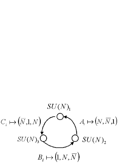
Figure 1: Gauge group $SU(N)_{1}\times SU(N)_{2}\times SU(N)_{3}$ and color representation assignments of the supersingleton fields $A_{i},\,B_{j},\,C_{\ell}$ in the $Q^{1,1,1}$ world volume gauge theory.

The global symmetry of the gauge theory is $SU(2)^{3}$, where each of the doublets of chiral fields transforms in the fundamental representation of one of the $SU(2)$’s.

Notice that we are considering $SU(N)$ gauge group and not the naively expected $U(N)$. The reason is that there is compelling evidence [3, 53, 39] that the $U(1)$ factors are washed out in the near horizon limit. Since in three dimensions $U(1)$ theories may give rise to CFT’s in the IR, it is an important point to check whether $U(1)$ factors are described by the $AdS$-solution or not. A first piece of evidence that the supergravity solutions are dual to $SU(N)$ theories, and not $U(N)$, comes from the absence in the KK spectrum (even in the maximal supersymmetric case) of KK modes corresponding to color trace of single fundamental fields of the CFT, which are non zero only for $U(N)$ gauge groups. A second evidence is the existence of states dual to baryonic operators in the non-perturbative spectrum of these Type II or M-theory compactifications; baryons exist only for $SU(N)$ groups. We will find baryons in the spectrum of both $Q^{1,1,1}$ and $M^{1,1,1}$: this implies that, for the compactifications discussed in this paper, the gauge group of the CFT is $SU(N)$.

In the non-abelian case, we expect that the generic point of the moduli space corresponds to N separated branes. Therefore, the space of vacua of the theory should reduce to the symmetrization of N copies of $Q^{1,1,1}$. To get rid of unwanted light non-abelian degrees of freedom, we would like to introduce, following [4], a superpotential for our theory. Unfortunately, the obvious candidate for this job

$$\epsilon^{ij}\epsilon^{mn}\epsilon^{pq}{\rm Tr}(A_{i}B_{m}C_{p}A_{j}B_{n}C_{q})$$ (4.2)

is identically zero. Here the close analogy with $T^{1,1}$ and reference [4] ends.

We consider now the spectrum of KK excitations of $Q^{1,1,1}$. The full spectrum of $Q^{1,1,1}$ is not known; however, the eigenvalues of the laplacian were computed in [37]. As shown in [35], the knowledge of the laplacian eigenvalues allows to compute the entire spectrum of hypermultiplets of the theory, corresponding to the chiral operators of the CFT. The result is that there is a chiral multiplet in the $(k/2,k/2,k/2)$ representation of $SU(2)^{3}$ for each integer value of k, with dimension $E_{0}=k$. We naturally associate these multiplets with the series of composite operators

$${\rm Tr}(ABC)^{k},$$ (4.3)

where the $SU(2)$’s indices are totally symmetrized. A first important result, following from the existence of these hypermultiplets in the KK spectrum, is that the dimension of the combination $ABC$ at the superconformal point must be 1.

We see that the prediction from the KK spectrum are in perfect agreement with the geometric discussion in the previous Section. Operators which are not totally symmetric in the flavor indices do not appear in the spectrum. The agreement with the proposed CFT, however, is only partial. The chiral operators predicted by supergravity certainly exist in the gauge theory. However, we can construct many more chiral operators which are not symmetric in flavor indices. They do not have any counterpart in the KK spectrum. The superpotential in the case of $T^{1,1}$ [4] had the double purpose of getting rid of the unwanted non-abelian degrees of freedom and of imposing, via the equations of motion, the total symmetrization for chiral and short operators which is predicted both by geometry and by supergravity. Here, we are not so lucky, since there is no superpotential. We can not consider superpotentials of dimension bigger than that considered before (for example, cubic or quartic in $ABC$) because the superpotential  (4.2) is the only one which has dimension compatible with the supergravity predictions. We need to suppose that all the non symmetric operators are not conformal primary. Since the relation between R-charge and dimension is only valid for conformal chiral operators, such operators are not protected and therefore may have enormous anomalous dimension, disappearing from the spectrum. Simple examples of chiral but not conformal operators are those obtained by derivatives of the superpotential. Since we do not have a superpotential here, we have to suppose that both the elimination of the unwanted colored massless states as well as the disappearing of the non-symmetric chiral operators emerges as a non-perturbative IR effect.

4.2 The case of $M^{1,1,1}$

Let us now consider $M^{1,1,1}$. The non-abelian theory is now $SU(N)\times SU(N)$ with chiral matter in the following representations of the gauge group

$$U^{i}\in Sym^{2}({\mathbb{C}}^{N})\otimes Sym^{2}({\mathbb{C}}^{N*}),\qquad\qquad V^{A}\in Sym^{3}({\mathbb{C}}^{N*})\otimes Sym^{3}({\mathbb{C}}^{N}).$$ (4.4)

The representations of the fundamental fields have been chosen in such a way that they reduce to the abelian theory discussed in the previous Section, match with the KK spectrum and imply the existence of baryons predicted by supergravity. Comparison with supergravity, which will be made soon, justifies, in particular, the choice of color symmetric representations.

The field content can be conveniently encoded in the quiver diagram in figure 2.

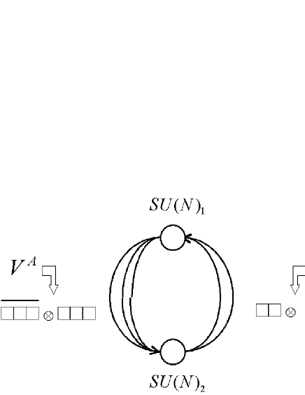
Figure 2: Gauge group $U(N)_{1}\times U(N)_{2}$ and color representation assignments of the supersingleton fields $V^{A}$ and $U^{i}$ in the $M^{1,1,1}$ world volume gauge theory.

The global symmetry of the gauge theory is $SU(3)\times SU(2)$, with the chiral fields $U$ and $V$ transforming in the fundamental representation of $SU(3)$ and $SU(2)$, respectively.

We next compare the expectations from gauge theory with the KK spectrum [35]. Let us start with the hypermultiplet spectrum (the full spectrum of KK modes will be discussed in Part II). There is exactly one hypermultiplet in the symmetric representation of $SU(3)$ with $3k$ indices and the symmetric representation of $SU(2)$ with $2k$ indices, for each integer $k\geq 1$. The dimension of the operator is $E_{0}=2k$. We naturally identify these states with the totally symmetrized chiral operators

$${\rm Tr}(U^{3}V^{2})^{k}.$$ (4.5)

One immediate consequence of the supergravity analysis is that the combination $U^{3}V^{2}$ has dimension 2 at the superconformal fixed point.

Once again, we are not able to write any superpotential of dimension 2. The natural candidate is the dimension two flavor singlet

$$\epsilon_{ijk}\epsilon_{AB}\left(U^{i}U^{j}U^{k}V^{A}V^{B}\right)_{\mbox{ color singlet}}$$ (4.6)

which however vanishes identically. There is no superpotential that might help in the elimination of unwanted light colored degrees of freedom and that might eliminate all the non symmetric chiral operators that we can construct out of the fundamental fields. Once again, we have to suppose that, at the superconformal fixed point in the IR, all the non totally symmetric operators are not conformal primaries.

4.3 The baryonic symmetries and the Betti multiplets

There is one important property that $M^{1,1,1}$, $Q^{1,1,1}$ and $T^{1,1}$ share. These manifolds have non-zero Betti numbers ($b_{2}=b_{5}=2$ for $Q^{1,1,1}$, $b_{2}=b_{5}=1$ for $M^{1,1,1}$ and $b_{2}=b_{3}=1$ for $T^{1,1}$). This implies the existence of non-perturbative states in the supergravity spectrum associated with branes wrapped on non-trivial cycles. They can be interpreted as baryons in the CFT [39, 6].

The existence of non-zero Betti numbers implies the existence of new global $U(1)$ symmetries which do not come from the geometrical symmetries of the coset manifold, as was pointed out long time ago. The massless vector multiplets associated with these symmetries were discovered and named Betti multiplets in [31, 26]. They have the property that the entire KK spectrum is neutral and only non-perturbative states can be charged. The massless vectors, dual to the conserved currents, arise from the reduction of the 11-dimensional 3-form along the non-trivial 2-cycles. This definition implies that non-perturbative objects made with M2 and M5 branes are charged under these $U(1)$ symmetries.

We can identify the Betti multiplets with baryonic symmetries. This was first pointed out in [59, 7] for the case of $T^{1,1}$ and discussed for orbifold models in [12]. The existence of baryons in the proposed CFT’s is due to the choice of $SU(N)$ (as opposed to $U(N)$) as gauge group. In the $SU(N)$ case, we can form the gauge invariant operators $\mbox{det}\,(A)$, $\mbox{det}\,(B)$ and $\mbox{det}\,(C)$ for $Q^{1,1,1}$ and $\mbox{det}\,(U)$ and $\mbox{det}\,(V)$ for $M^{1,1,1}$. The baryon symmetries act on fields in the same way as the $U(1)$ factors that we used for defining our abelian theories in Sections 3.1.1 and 3.1.2. They disappeared in the non-abelian theory associated to the conifolds, but the very same fact that they can be consistently incorporated in the theory means that they must exist as global symmetries. It is easy to check that no operator corresponding to KK states is charged under these $U(1)$’s. The reason is that the KK spectrum is made out with the combinations $X=ABC$ or $X=U^{3}V^{2}$ defined in Sections 3.1.1 and 3.1.2 which, by definition, are $U(1)$ invariant variables. The only objects that are charged under the $U(1)$ symmetries are the baryons.

Baryons have dimensions which diverge with $N$ and can not appear in the KK spectrum. They are indeed non-perturbative objects associated with wrapped branes [39, 6]. We see that the baryonic symmetries have the right properties to be associated with the Betti multiplets: the only charged objects are non-perturbative states. This identification can be strengthened by noticing that the only non-perturbative branes in M-theory have an electric or magnetic coupling to the eleven dimensional three-form. Since for our manifolds, both $b_{2}$ and $b_{5}$ are greater than 0, we have the choice of wrapping both M2 and M5-branes. M2 branes wrapped around a non-trivial two-cycle are certainly charged under the massless vector in the Betti multiplet which is obtained by reducing the three-form on the same cycle. Since a non-trivial 5-cycle is dual to a 2-cycle, a similar remark applies also for M5-branes. We identify M5-branes as baryons because they have a mass (and therefore a conformal dimension) which goes like $N$, as discussed in Section 5.2.

What follows from the previous discussion and is probably quite general, is that there is a close relation between the $U(1)$’s entering the brane construction of the gauge theory, the baryonic symmetries and the Betti multiplets. The previous remarks apply as well to CFT associated with orbifolds of $AdS_{4}\times S^{7}$. In the case of $T^{1,1}$,$Q^{1,1,1}$ and $M^{1,1,1}$, the baryonic symmetries are also directly related to the $U(1)$’s entering the toric description of the manifold.

4.4 Non trivial results from supergravity: a discussion

In the previous Sections, we proposed non-abelian theories as dual candidates for the M theory compactification on $Q^{1,1,1}$ and $M^{1,1,1}$. We also pointed out the difficulties related to the existence of more candidate conformal chiral operators than those expected from the KK spectrum analysis. We have no good arguments for claiming that these non flavor symmetric operators disappear in the IR limit. If they survive, this certainly signals the need for modifying our guess for the dual CFT’s. In the latter case, new fields may be needed. The theories we wrote down are based on the minimal assumption that there is no superpotential in the abelian case; if we relax this assumption, more complicated candidate dual gauge theories may exist. In the case of $T^{1,1}$, the CFT was identified in two different ways, by using the previous section arguments and also by describing the conifold as a deformation of an orbifold singularity. Since orbifold CFT can be often identified using standard techniques [10], this approach has the advantage of unambiguously identifying the conifold CFT. It would be interesting to find an analogous procedure for the case of $AdS_{4}$. It would provide a CFT which flows in the IR to the conifold theory after a deformation [4, 12] and it would help in checking whether new fields are necessary or not for a correct description of the CFT’s. Attempts to find associated orbifold models in the case of $Q^{1,1,1}$ have been made in [42, 43]; the precise relation with our approach is still to be clarified .

In any event, whatever is the microscopic description of the gauge theory flowing to the superconformal points in the IR, it is reasonable to think all the relevant degrees of freedom at the superconformal fixed point corresponding to the M theory on $Q^{1,1,1}$ and $M^{1,1,1}$ has been identified in the previous geometrical analysis. We will make, from now on, the assumption that the fundamental singletons of the CFT for $Q^{1,1,1}$ are the fields $A,B,C$ and for $M^{1,1,1}$ the fields $U,V$ with the previously discussed assignment of color and flavor indices and that they always appear in totally symmetrized flavor combinations. Given this simple assumption, inherited from the geometry of the conifolds, we can make several non-trivial comparisons between the expectation of a CFT (in which the singletons are totally symmetrized in flavor) and the supergravity prediction. We leave for future work the clarification of the dynamical mechanism (or possible modification of the three-dimensional gauge theories) for suppressing the non-symmetric operators as well as the search for a RG flow from an orbifold model.

We already discussed the chiral operators of the two CFT’s. We obtained two main results from this analysis. The first one states that all chiral operators are symmetrized in flavor indices. The second one, more quantitative, predicts the conformal dimension of some composite objects. When appearing in gauge invariant chiral operators, the symmetrized combinations $ABC$ and $U^{3}V^{2}$ have dimensions 1 and 2, respectively.

Having this information, there are two types of important and non-trivial checks that we can make:

• The full spectrum of KK excitations should match with composite operators in the CFT. Specifically, besides the hypermultiplets, there are many other short multiplets in the spectrum. All these multiplets should match with CFT operators with protected dimension. This will be verified in Sections 6.3, 6.4.

• We can determine the dimension of a baryon operator by computing the volume of the cycle the M5-brane is wrapping, following [6]. From this, we can determine the dimension of the fundamental fields of the CFT. This can be compared with the expectations from the KK spectrum. The agreement of the two methods can be considered as a non-trivial check of the AdS/CFT correspondence. This will be discussed in Section 5.

Leaving the actual computation and detailed comparison of spectra for the second Part of this paper, here we summarize the results of our analysis.

The spectrum of $M^{1,1,1}$ is completely known [35]. This allows a detailed comparison of all the states in supergravity with CFT operators. Besides the hypermultiplets, which fit the quantum field theory expectations in a straightforward manner, there are various series of multiplets which are short and therefore protected. An highly non-trivial result is that we will be able to identify all the KK short multiplets with candidate CFT operators of requested quantum numbers and conformal dimension. Most of them can be obtained by tensoring conserved currents with chiral operators. The same analysis was done for $T^{1,1}$ in [7]. In ${\cal N}=2$ supersymmetric compactifications, the KK spectrum contains both short and long multiplets. We will notice that there is a common pattern in $Q^{1,1,1}$, $M^{1,1,1}$ as well as in $T^{1,1}$, of long multiplets which have rational and protected dimension. In particular, following [7], we can identify in all these models rational long gravitons with products of the stress energy tensor, conserved currents and chiral operators. We suspect the existence of some field theoretical reason for the unexpected protected dimension of these operators.

The dimension of the fundamental fields $A,B,C$ and $U,V$ at the superconformal point can be computed and compared with the KK spectrum prediction. In the KK spectrum, these fields always appear in particular combinations. For example, we already know that $ABC$ has dimension 1 and $U^{3}V^{2}$ has dimension 2. $A,B,C$ have clearly the same dimension $1/3$ since there is a permutation symmetry. But, what’s about $U$ or $V$? From the CFT point of view, we expect the existence of several baryon operators: $\mbox{det}\,A$, $\mbox{det}\,B$, $\mbox{det}\,C$ for $Q^{1,1,1}$ and $\mbox{det}\,U$, $\mbox{det}\,V$ for $M^{1,1,1}$. All of them should correspond to M5-branes wrapped on supersymmetric five-cycles of $M^{7}$. We can determine the dimension of the single fields $A$ or $U$ by computing the mass of a wrapped M5-brane [6]. This amounts to identifying a supersymmetric 5-cycle and computing its volume. The details of the identification of the cycles, the actual computation of normalizations and volumes will be discussed in Sections 7.1.5, 7.1.6, 7.1.7, 7.2.4. Here we give the results.

In the case of $Q^{1,1,1}$, since the manifold is a $U(1)$ fibration over $S^{2}\times S^{2}\times S^{2}$, we can identify three distinct supersymmetric 5-cycles by considering the 5-manifolds obtained by selecting a particular point in one of the three $S^{2}$. The computation of volumes predicts a common dimension $N/3$ for the three candidate baryons $\mbox{det}\,A$, $\mbox{det}\,B$ and $\mbox{det}\,C$. We conclude that the three fundamental fields $A,B,C$ have dimension $1/3$. Both the dimension and the flavor representation of these baryons, which will be determined in Section 5, are in agreement with the KK expectations.

In the case of $M^{1,1,1}$, there are two supersymmetric cycles. $M^{1,1,1}$ is a $U(1)$ fibration over ${\mathbb{P}}^{1}\times{\mathbb{P}}^{2*}$. A first non-trivial supersymmetric 5-cycle is obtained by selecting a point in ${\mathbb{P}}^{1}$; the associated baryon carries flavor indices of $SU(2)$. A second 5-cycle is obtained by selecting a ${\mathbb{P}}^{1}$ inside ${\mathbb{P}}^{2*}$ (see Section 7.1.6); the associated baryon only carries indices of $SU(3)$. We can determine the dimensions of the baryons $\mbox{det}\,U$ and $\mbox{det}\,V$, by computing the volume of these 5-cycles, and we find $4N/9$ and $N/3$, predicting dimension $4/9$ and $1/3$ for $U$ and $V$. This strange numbers are nevertheless in perfect agreement with the KK expectation: the dimension of $U^{3}V^{2}$ is

$$3\times{4\over 9}+2\times{1\over 3}=2,$$ (4.7)

as expected from the KK analysis. We find that this is quite a non-trivial and remarkable check of the AdS/CFT correspondence.

Let us finish this brief discussion, by considering the issue of possible marginal deformations of our CFT’s. A natural question is whether the proposed CFT’s belong to a line of fixed points or not. We already noticed that in three dimensions there is no analogous of the $AdS_{5}$ dilaton and therefore we may expect that, in general, the CFT’s related to $AdS_{4}$ are isolated fixed points, if we pretend to maintain the global symmetry and the number of supersymmetries of our CFT’s. If there is some marginal deformation we should be able to see it in the KK spectrum as an operator of dimension 3. We can certainly exclude the existence of marginal deformations that preserves the global symmetries of the fixed point, at least for $M^{1,1,1}$ where the KK spectrum is completely known: there is no flavor singlet scalar of dimension 3 in the supergravity spectrum. Other possible sources for exact marginal deformations preserving the global symmetries come from non-trivial cycles. In $T^{1,1}$, for example, the second complex marginal deformation arises from the zero-mode value of the B field on the non-trivial two-cycles of the manifold. In our case, however, an analogous phenomenon requires reducing the three form on a non-trivial 3-cycle, which does not exist. It is likely that marginal deformations which break the flavor symmetry but maintain the same number of supersymmetries exist in all these models, since non flavor singlet multiplets with highest component of dimension three can be found in the KK spectrum; whether these deformation are truly marginal or not needs to be investigated in more details.

The rest of this paper will be devoted to an exhaustive comparison between quantum field theory and supergravity and to a detailed description of the geometry involved in such a comparison.

Part II Comparison between KK spectra and the gauge theory

5 Dimension of the supersingletons and the baryon operators

As we have anticipated in the introduction, the first basic check on our conjectured conformal gauge theories comes from a direct computation of the conformal weight of the singleton superfields

$$\mbox{singleton superfields}=\cases{\begin{array}[]{cccl}U^{i}&V^{A}&\hbox{}\hfil&\mbox{in the $M^{1,1,1}$ theory}\\ \hbox{}\hfil&\hbox{}\hfil&\hbox{}\hfil\\ A_{i}&B_{j}&C_{\ell}&\mbox{in the $Q^{1,1,1}$ theory}\end{array}}$$ (5.1)

whose color index structure and $\theta$-expansion are explicitly given in the later formulae (6.1), (6.3). If the non–abelian gauge theory has the $SU(N)\times\dots\times SU(N)$ gauge groups illustrated by the quiver diagrams of fig.s 1 and 2, then we can consider the following chiral operators:

$$\mbox{det}U \equiv U_{i_{1}|\Lambda^{1}_{1}\Sigma^{1}_{1}}^{\Lambda^{2}_{1}\Sigma^{2}_{1}}\,\dots\,U_{i_{N}|\Lambda^{1}_{N}\Sigma^{1}_{N}}^{\Lambda^{2}_{N}\Sigma^{2}_{N}}\,\epsilon^{\Lambda^{1}_{1}\dots\Lambda^{1}_{N}}\,\epsilon^{\Sigma^{1}_{1}\dots\Sigma^{1}_{N}}\epsilon_{\Lambda^{2}_{1}\dots\Lambda^{2}_{N}}\,\epsilon_{\Sigma^{2}_{1}\dots\Sigma^{2}_{N}}$$ (5.2)

$$\mbox{det}V \equiv V_{A_{1}|\Lambda^{1}_{1}\Sigma^{1}_{1}\Gamma^{1}_{1}}^{\Lambda^{2}_{1}\Sigma^{2}_{1}\Gamma^{2}_{1}}\,\dots\,V_{A_{N}|\Lambda^{1}_{N}\Sigma^{1}_{N}\Gamma^{1}_{N}}^{\Lambda^{2}_{N}\Sigma^{2}_{N}\Gamma^{2}_{N}}\,\epsilon^{\Lambda^{1}_{1}\dots\Lambda^{1}_{N}}\,\epsilon^{\Sigma^{1}_{1}\dots\Sigma^{1}_{N}}\epsilon^{\Gamma^{1}_{1}\dots\Gamma^{1}_{N}}\epsilon_{\Lambda^{2}_{1}\dots\Lambda^{2}_{N}}\,\epsilon_{\Sigma^{2}_{1}\dots\Sigma^{2}_{N}}\epsilon_{\Gamma^{2}_{1}\dots\Gamma^{2}_{N}}$$ (5.3)

$$\mbox{det}A \equiv A_{i_{1}|\Lambda^{1}_{1}}^{\Lambda^{2}_{1}}\,\dots\,A_{i_{N}|\Lambda^{1}_{N}}^{\Lambda^{2}_{N}}\,\epsilon^{\Lambda^{1}_{1}\dots\Lambda^{1}_{N}}\,\epsilon_{\Lambda^{2}_{1}\dots\Lambda^{2}_{N}}$$ (5.4)

$$\mbox{det}B \equiv B_{i_{1}|\Lambda^{2}_{1}}^{\Lambda^{3}_{1}}\,\dots\,B_{i_{N}|\Lambda^{2}_{N}}^{\Lambda^{3}_{N}}\,\epsilon^{\Lambda^{2}_{1}\dots\Lambda^{2}_{N}}\,\epsilon_{\Lambda^{3}_{1}\dots\Lambda^{3}_{N}}$$ (5.5)

$$\mbox{det}C \equiv C_{i_{1}|\Lambda^{3}_{1}}^{\Lambda^{1}_{1}}\,\dots\,C_{i_{N}|\Lambda^{3}_{N}}^{\Lambda^{1}_{N}}\,\epsilon^{\Lambda^{3}_{1}\dots\Lambda^{3}_{N}}\,\epsilon_{\Lambda^{1}_{1}\dots\Lambda^{1}_{N}}.$$ (5.6)

If these operators are truly chiral primary fields, then their conformal dimensions are obviously given by

$$\begin{array}[]{ccccccccccc}h[\mbox{det}\,U]&=&h[U]\,\times\,N&;&h[\mbox{det}\,V]&=&h[V]\,\times\,N&\hbox{}\hfil&\hbox{}\hfil&\hbox{}\hfil&\hbox{}\hfil\\ h[\mbox{det}\,A]&=&h[A]\,\times\,N&;&h[\mbox{det}\,B]&=&h[B]\,\times\,N&;&h[\mbox{det}\,C]&=&h[C]\,\times\,N\\ \end{array}$$ (5.7)

and their flavor representations are:

$$\mbox{det}\,U \Rightarrow (M_{1}=N,M_{2}=0,J=0),$$ (5.8)

$$\mbox{det}\,V \Rightarrow (M_{1}=0,M_{2}=0,J=N/2),$$ (5.9)

$$\mbox{det}\,A \Rightarrow (J_{1}=N/2,J_{2}=0,J_{3}=0),$$ (5.10)

$$\mbox{det}\,B \Rightarrow (J_{1}=0,J_{2}=N/2,J_{3}=0),$$ (5.11)

$$\mbox{det}\,C \Rightarrow (J_{1}=0,J_{2}=0,J_{3}=N/2),$$ (5.12)

where the conventions for the flavor representation labeling are those explained later in eq.s (6.15), (6.18).

The interesting fact is that the conformal operators (5.2,…,5.6) can be reinterpreted as solitonic supergravity states obtained by wrapping a $5$–brane on a non–trivial supersymmetric $5$–cycle. This gives the possibility of calculating directly the mass of such states and, as a byproduct, the conformal dimension of the individual supersingletons. All what is involved is a geometrical information, namely the ratio of the volume of the $5$–cycles to the volume of the entire compact $7$–manifold. In addition, studying the stability subgroup of the supersymmetric $5$–cycles, we can also verify that the gauge–theory predictions (5.8,…,5.12) for the flavor representations are the same one obtains in supergravity looking at the state as a wrapped solitonic $5$–brane.

To establish these results we need to derive a general mass–formula for baryonic states corresponding to wrapped $5$–branes. This formula is obtained by considering various relative normalizations.

5.1 The M2 brane solution and normalizations of the seven manifold metric and volume

Using the conventions and normalizations of [52, 55] for $D=11$ supergravity and for its Kaluza Klein expansions, a Freund Rubin solution on $AdS_{4}\times M^{7}$ is described by the following three equations:

$$\begin{array}[]{ccccccc}R^{ab}&=&-16e^{2}\,E^{a}\wedge E^{b}&\Rightarrow&R^{ab}_{cb}&=&-24\,e^{2}\,\delta^{a}_{c}\\ R^{\hat{a}\hat{b}}&=&R^{\hat{a}\hat{b}}_{\hat{c}\hat{d}}\,B^{\hat{c}}\,B^{\hat{d}}&\mbox{with}&R^{\hat{a}\hat{b}}_{\hat{c}\hat{b}}&=&12\,e^{2}\,\delta^{\hat{a}}_{\hat{c}}\\ F^{[4]}&=&e\,\varepsilon_{abcd}\,E^{a}\,\wedge\,E^{b}\,\wedge\,E^{c}\,\wedge\,E^{d}\,,&\hbox{}\hfil&\hbox{}\hfil&\hbox{}\hfil&\hbox{}\hfil\end{array}$$ (5.13)

where $E^{a}$ ($a=0,1,2,3$) is the vielbein of anti de Sitter space $AdS_{4}$, $R^{ab}$ is the corresponding curvature $2$–form, $B^{\hat{a}}$ ($\hat{a}=4,\dots,10$) is the vielbein of $M^{7}$ and $R^{\hat{a}\hat{b}}$ is the corresponding curvature. The parameter $e$, expressing the vev of the $4$–form field strength, is called the Freund Rubin parameter. In these normalizations, both the internal and space–time vielbeins do not have their physical dimension of a length $[E^{a}]_{phys}=[B^{\hat{a}}]_{phys}=\ell$, since one has reabsorbed the Planck length $\ell_{P}$ into their definition by working in natural units where the $D=11$ gravitational constant $G_{11}$ has been set equal to $1\over 8\pi$. Physical units are reinstalled through the following rescaling:

$$E^{a} = \frac{1}{\kappa^{2/9}}\,\hat{E}^{a},$$

$$B^{a} = \frac{1}{\kappa^{2/9}}\,\hat{B}^{a},$$

$$F^{[4]}_{abcd} = \kappa^{11/9}\,\hat{F}^{[4]}_{abcd},$$

$$\kappa^{2} = 8\pi G_{11}=\frac{(2\pi)^{8}}{2}\,\ell_{P}^{9}.$$ (5.14)

After such a rescaling, the relations between the Freund Rubin parameter and the curvature scales for both $AdS_{4}$ and $M^{7}$ become

$$\mbox{Ricci}_{\mu\nu}^{AdS} = -2\,\Lambda\,g_{\mu\nu}$$ (5.15)

$$\mbox{Ricci}_{\hat{\mu}\hat{\nu}}\ = \Lambda g_{\hat{\mu}\hat{\nu}}$$ (5.16)

$$\Lambda \stackrel{{\scriptstyle\mbox{\scriptsize def}}}{{=}} 24\,\frac{e^{2}}{\kappa^{4/9}}.$$ (5.17)

Note that in eq. (5.17) we have used the normalization of the Ricci tensor which is standard in the general relativity literature and is twice the normalization of the Ricci tensor $R^{ab}_{cb}$ appearing in eq. (5.13). Furthermore eq.s (5.13) were written in flat indices while eq.s (5.15, 5.16) are written in curved indices.

For our further reasoning, it is convenient to write the anti de Sitter metric in the solvable coordinates [21, 1]:

$$ds^{2}_{AdS_{4}} = R_{AdS}^{2}\left[\rho^{2}\left(-dt^{2}+dx_{1}^{2}+dx_{2}^{2}\right)+\frac{d\rho^{2}}{\rho^{2}}\right],$$

$$\mbox{Ricci}_{\mu\nu}^{AdS} = -\frac{3}{R^{2}_{AdS}}\,g_{\mu\nu},$$

which yields the relation

$$R_{AdS}=\frac{\kappa^{2/9}}{4\,e}=\frac{1}{2}\,\sqrt{\frac{6}{\Lambda}}.$$ (5.19)

Next, following [48] we can consider the exact M2–brane solution of $D=11$ supergravity that has the cone ${\cal C}(M^{7})$ over $M^{7}$ as transverse space. The $D=11$ bosonic action can be written as

$$I_{11}=\int d^{11}x\sqrt{-g}~{}({R\over\kappa^{2}}-3\,\hat{F}^{2}_{[4]})+{288}\sigma\int\hat{F}_{[4]}\wedge\hat{F}_{[4]}\wedge\hat{A}_{[3]}$$ (5.20)

(where the coupling constant for the last term is $\sigma=\kappa$) and the exact $M2$–brane solution is as follows:

$$ds^{2}_{M2} = \left(1+\frac{k}{r^{6}}\right)^{-2/3}(-dt^{2}+dx_{1}^{2}+dx_{2}^{2})+\left(1+\frac{k}{r^{6}}\right)^{1/3}\,ds^{2}_{cone},$$

$$ds^{2}_{cone} = dr^{2}+r^{2}\frac{\Lambda}{6}ds^{2}_{M^{7}},$$

$$A^{[3]} = dt\wedge dx_{1}\wedge dx_{2}\,\left(1+\frac{k}{r^{6}}\right)^{-1},$$ (5.21)

where $ds^{2}_{M^{7}}$ is the Einstein metric on $M^{7}$, with Ricci tensor as in eq. (5.17), and $ds^{2}_{cone}$ is the corresponding Ricci flat metric on the associated cone. When we go near the horizon, $r\to 0$, the metric (5.21) is approximated by

$$ds^{2}_{M2}\approx r^{4}(-dt^{2}+dx_{1}^{2}+dx_{2}^{2})\,k^{-2/3}+k^{1/3}\,\frac{dr^{2}}{r^{2}}+k^{1/3}\,\frac{\Lambda}{6}\,ds_{M^{7}}^{2}.$$ (5.22)

The Freund Rubin solution $AdS_{4}\times M^{7}$ is obtained by setting

$$\rho={2\over\sqrt{k}}\,r^{2}$$ (5.23)

and by identifying

$$R_{AdS}=\frac{k^{1/6}}{2}\quad\Leftrightarrow\quad\Lambda=6k^{-1/3}.$$ (5.24)

5.2 The dimension of the baryon operators

Having fixed the normalizations, we can now compute the mass of a M5-brane wrapped around a non-trivial supersymmetric cycle of $M^{7}$ and the conformal dimension of the associated baryon operator.

The parameter $k$ appearing in the M2-solution is obviously proportional to the number $N$ of membranes generating the $AdS$-background and, by dimensional analysis, to $l_{P}^{6}$. The exact relation for the maximally supersymmetric case $AdS_{4}\times S^{7}$ can be found in [1] and reads

$$R_{AdS}={l_{P}\over 2}\left(2^{5}\pi^{2}N\right)^{1/6}\quad\Leftrightarrow\quad k=2^{5}\pi^{2}Nl_{P}^{6}.$$ (5.25)

We can easily adapt this formula to the case of $AdS_{4}\times M^{7}$ by noticing that, by definition, the number of M2-branes $N$ is determined by the flux of the RR three-form through $M^{7}$, $\int_{M^{7}}*F^{[4]}$. As a consequence, $N$ and the volume of $M^{7}$ will appear in all the relevant formulae in the combination $N/{\rm Vol}(M^{7})$. We therefore obtain the general formula

$$\sqrt{{\Lambda\over 6}}=\left({{\rm Vol}(M^{7})\over{\rm Vol}(S^{7})}\right)^{1/6}{1\over l_{P}(2^{5}\pi^{2}N)^{1/6}}.$$ (5.26)

We can now consider the solitonic particles in $AdS_{4}$ obtained by wrapping M2- and M5-branes on the non-trivial 2- and 5-cycles of $M^{7}$, respectively. They are associated with boundary operators with conformal dimensions that diverge in the large $N$ limit. The exact dependence on $N$ can be easily estimated. Without loss of generality, we can put $\Lambda=1$ using a conformal transformation; its only role in the game is to fix a reference scale and it will eventually cancel in the final formulae. The mass of a p-brane wrapped on a p-cycle is given by $T_{p}\times{\rm Vol(p-cycle)}\sim l_{P}^{-\left(p+1\right)}\Lambda^{-{p\over 2}}\sim l_{P}^{-\left(p+1\right)}$. Once the mass of the non-perturbative states is known, the dimension $E_{0}$ of the associated boundary operator is given by the relation $m^{2}=(2\Lambda/3)(E_{0}-1)(E_{0}-2)\sim 2E_{0}^{2}/3$. From equation  (5.26) we learn that $l_{P}\sim N^{-1/6}$. We see that M2-branes correspond to operators with dimension $\sqrt{N}$ while M5-branes to operators with dimension of order $N$. The natural candidates for the baryonic operators we are looking for are therefore the wrapped five-branes.

We can easily write a more precise formula for the dimension of the baryonic operator associated with a wrapped M5-brane, following the analogous computation in [6]. For this, we need the exact expression for the M5 tension which can be found, for example, in [56]. We find

$$m={1\over(2\pi)^{5}l_{P}^{6}}{\rm Vol(5-cycle)}.$$ (5.27)

Using equation (5.26) and the above discussed relation between mass of the bulk particle and conformal dimension of the associated boundary operators, we obtain the formula for the dimension of a baryon,

$$E_{0}={\pi N\over\Lambda}{{\rm Vol(5-cycle)}\over{\rm Vol}(M^{7})},$$ (5.28)

where the volume is evaluated with the internal metric normalized so that (5.16) is true.

As a check, we can compute the dimension of a Pfaffian operator in the ${\cal N}=8$ theory with gauge group $SO(2N)$. The theory contains adjoint scalars which can be represented as antisymmetric matrices $\phi_{ij}$ and we can form the gauge invariant baryonic operator $\epsilon_{i_{1},...,i_{2N}}\phi_{i_{1}i_{2}}....\phi_{i_{2N-1}i_{2N}}$ with dimension $N/2$. The internal manifold is ${\mathbb{RP}}^{7}$ [39, 57], a supersymmetric preserving ${\mathbb{Z}}_{2}$ projection of original $AdS_{4}\times S^{7}$ case, corresponding to the $SU(N)$ gauge group. We obtain the Pfaffian by wrapping an M5-brane on a ${\mathbb{RP}}^{5}$ submanifold. Equation  (5.28) gives

$$E_{0}={\pi N\over\Lambda}{{\rm Vol}{\mathbb{RP}}^{5}\over{\rm Vol}{\mathbb{RP}}^{7}}={\pi N\over\Lambda}{{\rm Vol}S^{5}\over{\rm Vol}S^{7}}=N/2,$$ (5.29)

as expected.

Let us now apply the above formula to the case of the theories $M^{1,1,1}$ and $Q^{1,1,1}$. In Section 7.1.5 we show that the Sasakian manifold $M^{1,1,1}$ has two homology $5$ cycles ${\cal C}^{1}$ and ${\cal C}^{2}$ (see their definition in eq.s (7.102, 7.105)) belonging to the unique homology class, but distinguished by their stability subgroups $H({\cal C}^{1,2})\subset SU(3)\times SU(2)\times U(1)$, respectively given in eq.s (7.112) and (7.113). Furthermore in Section 7.1.7 we show that, after being pulled back to these cycles, the $\kappa$–supersymmetry projector of the $5$–brane is non vanishing on the killing spinors of the supersymmetries preserved by $M^{1,1,1}$. This proves that the $5$–brane wrapped on these cycles is a $BPS$–state with mass equal to its own $6$–form charge or, briefly stated, that the $5$–cycles are supersymmetric. Wrapping the $5$–brane on these cycles, we obtain good candidates for the supergravity representation of the baryonic operators (5.2) and (5.3). To understand which is which, we have to decide the flavor representation. This is selected by the stability subgroup $H({\cal C}^{i})$. Following an argument introduced by Witten [39], the collective degrees of freedom $c$ of the wrapped $5$–brane soliton live on the coset manifold $G/H({\cal C}^{i})$, where $G$ is the isometry group of $M^{7}$. The wave–function $\Psi(c)$ of the soliton must be expanded in harmonics on $G/H({\cal C}^{i})$ characterized by having charge $N$ under the baryon number $U(1)_{B}\subset H({\cal C}^{i})$. Minimizing the energy operator (the laplacian) on such harmonics one obtains the corresponding $G$ representation and hence the flavor assignment of the baryon. In Section 7.1.6, applying such a discussion to the pair of $5$–cycles under consideration, we find that they are respectively associated with the flavor representations

$${\cal C}^{1} \Leftrightarrow (M_{1}=0,M_{2}=0,J=N/2)$$ (5.30)

$${\cal C}^{2} \Leftrightarrow (M_{1}=N,M_{2}=0,J=0)$$ (5.31)

(see eq.s (7.119), and (7.120)). Comparing eq.s (5.30, 5.31) with eq.s (5.8, 5.9), we see that the first cycle is a candidate to represent the operator $\mbox{det}\,U$, while the second cycle is a candidate to represent the operator $\mbox{det}\,V$. The final check comes from the evaluation of the cycle volumes. This is done in eq.s (7.106) and (7.107). Inserting these results and the formula (7.108) for the $M^{1,1,1}$ volume into the general formula (5.28), we obtain

$$E_{0}\left(\mbox{det}\,U\right) = {\textstyle\frac{4}{9}}\,\times\,N\quad\Rightarrow h[U]={\textstyle\frac{4}{9}},$$ (5.32)

$$E_{0}\left(\mbox{det}\,U\right) = {\textstyle\frac{1}{3}}\,\times\,N\quad\Rightarrow h[V]={\textstyle\frac{1}{3}}.$$ (5.33)

As we have already stressed, it is absolutely remarkable that these non–perturbatively determined conformal weights are in perfect agreement with the Kaluza Klein spectra as we show in Section 6.

In Section 7.2.4 we show that the manifold $Q^{1,1,1}$ has three homology cycles ${\cal C}^{A,B,C}$ permuted by the $\Sigma_{3}$ symmetry that characterizes this manifold. Their volume is calculated in eq. (7.164) and their stability subgroups in eq. (7.167). Applying the same argument as above, we show in Section 7.2.4 that the flavor representations associated with these three cycles are indeed those of eq.s (5.10,…,5.12), so that these three cycles are candidates as supergravity representations of the conformal operators ${\rm det}\,A$, ${\rm det}\,B$, and ${\rm det}\,C$. Inserting the volume (7.164) of the cycles and the volume (7.165) of $Q^{1,1,1}$ into the baryon formula (5.28), we find that the conformal dimension of the $A,B,C$ supersingletons is

$$h[A_{i}]=h[B_{j}]=h[C_{\ell}]=\frac{1}{3}$$ (5.34)

as stated in eq. (7.169).

6 Conformal superfields of the $M^{1,1,1}$ and $Q^{1,1,1}$ theories

Starting from the choice of the supersingleton fields and of the chiral ring (inherited from the geometry of the compact Sasakian manifold), we can build all sort of candidate conformal superfields for both theories $M^{1,1,1}$ and $Q^{1,1,1}$. In the first case, where the full spectrum of $Osp(2|4)\times SU(3)\times SU(2)$ supermultiplets has already been determined through harmonic analysis [35], relying on the conversion vocabulary between $AdS_{4}$ bulk supermultiplets and boundary superfields established in [36], we can make a detailed comparison of the Kaluza Klein predictions with the candidate conformal superfields available in the gauge theory. In particular we find the gauge theory interpretation of the entire spectrum of short multiplets. The corresponding short superfields are in the right $SU(3)\times SU(2)$ representations and have the right conformal dimensions. Applying the same scheme to the case of $Q^{1,1,1}$, we can use the gauge theory to make predictions about the spectrum of short multiplets one should find in Kaluza Klein harmonic expansions. The partial results already known from harmonic analysis on $Q^{1,1,1}$ are in agreement with these predictions.

In addition, looking at the results of [35], one finds that there is a rich collection of long multiplets whose conformal dimensions are rational and seem to be protected from acquiring quantum corrections. This is in full analogy with results obtained in the four–dimensional theory associated with the $T^{1,1}$ manifold [5, 7]. Actually, we find an even larger class of such rational long multiplets. For a subclass of them the gauge theory interpretation is clear while for others it is not immediate. Their presence, which seems universal in all coset models, indicates some general protection mechanism that has still to be clarified.

Using the notations of [36], the singleton superfields of the $M^{1,1,1}$ theory are the following ones:

$$U^{i|\Lambda\Sigma}_{\phantom{i|\Lambda\Sigma}\underline{\Gamma\Delta}}(x,\theta) = u^{i|\Lambda\Sigma}_{\phantom{i|\Lambda\Sigma}\underline{\Gamma\Delta}}(x)+\left(\lambda_{u}^{\alpha}\right)^{i|\Lambda\Sigma}_{\phantom{i|\Lambda\Sigma}\underline{\Gamma\Delta}}(x)~{}\theta^{+}_{\alpha},$$

$$V^{A|\underline{\Gamma\Delta\Theta}}_{\phantom{A|\underline{\Gamma\Delta\Theta}}\Lambda\Sigma\Pi}(x,\theta) = v^{A|\underline{\Gamma\Delta\Theta}}_{\phantom{A|\underline{\Gamma\Delta\Theta}}\Lambda\Sigma\Pi}(x)+\left(\lambda_{v}^{\alpha}\right)^{A|\underline{\Gamma\Delta\Theta}}_{\phantom{A|\underline{\Gamma\Delta\Theta}}\Lambda\Sigma\Pi}(x)~{}\theta^{+}_{\alpha},$$ (6.1)

where $(i,A)$ are $SU(3)\times SU(2)$ flavor indices, $(\Lambda,\underline{\Lambda})$ are $SU(N)\times SU(N)$ color indices while $\alpha$ is a world volume spinorial index of $SO(1,2)$. The supersingletons are chiral superfields, so they satisfy $E_{0}=|y_{0}|$.

$U^{i}$ is in the fundamental representation ${\bf 3}$ of $SU(3)_{\rm flavor}$ and in the $\left(\Box\!\Box,{\Box\!\Box}^{\star}\right)$ of $(SU(N)\times SU(N))_{\rm color}$. $V^{A}$ is in the fundamental representation ${\bf 2}$ of $SU(2)_{\rm flavor}$ and in the $\left({\Box\!\Box\!\Box}^{\star},\Box\!\Box\!\Box\right)$ of $\left(SU(N)\times SU(N)\right)_{\rm color}$. In eq.s (6.1) we have followed the conventions that lower $SU(N)$ indices transform in the fundamental representation, while upper $SU(N)$ indices transform in the complex conjugate of the fundamental representation.

Studying the non perturbative baryon state, obtained by wrapping the $5$–brane on the supersymmetric cycles of $M^{1,1,1}$, we have unambiguously established the conformal weights of the supersingletons (or, more precisely, the conformal weights of the Clifford vacua $u,v$) that are:

$$E_{0}(u)=y_{0}(u)={4\over 9},~{}~{}~{}E_{0}(v)=y_{0}(v)={1\over 3}.$$ (6.2)

For the $Q^{1,1,1}$ theory the singleton superfields are instead the following ones:

$$A^{\phantom{\Lambda_{1}}\Gamma_{2}}_{i_{1}|\Lambda_{1}}(x,\theta) = a^{\phantom{\Lambda_{1}}\Gamma_{2}}_{i_{1}|\Lambda_{1}}(x)+\left(\lambda_{a}^{\alpha}\right)^{\phantom{\Lambda_{1}}\Gamma_{2}}_{i_{1}|\Lambda_{1}}(x)~{}\theta^{+}_{\alpha},$$

$$B^{\phantom{\Lambda_{2}}\Gamma_{3}}_{i_{2}|\Lambda_{2}}(x,\theta) = b^{\phantom{\Lambda_{2}}\Gamma_{3}}_{i_{2}|\Lambda_{2}}(x)+\left(\lambda_{b}^{\alpha}\right)^{\phantom{\Lambda_{2}}\Gamma_{3}}_{i_{2}|\Lambda_{2}}(x)~{}\theta^{+}_{\alpha},$$

$$C^{\phantom{\Lambda_{3}}\Gamma_{1}}_{i_{3}|\Lambda_{3}}(x,\theta) = c^{\phantom{\Lambda_{3}}\Gamma_{1}}_{i_{3}|\Lambda_{3}}(x)+\left(\lambda_{c}^{\alpha}\right)^{\phantom{\Lambda_{3}}\Gamma_{1}}_{i_{3}|\Lambda_{3}}(x)~{}\theta^{+}_{\alpha},$$ (6.3)

where $i_{\ell}$ $(\ell=1,2,3)$ are flavor indices of $SU(2)_{1}\times SU(2)_{2}\times SU(2)_{3}$, while $\Lambda_{\ell}$ $(\ell=1,2,3)$ are color indices of $SU(N)_{1}\times SU(N)_{2}\times SU(N)_{3}$. Also in this case we know the conformal dimension of the supersingleton fields through the calculation of the conformal dimension of the baryon operators. We have:

$$E_{0}(a)=E_{0}(b)=E_{0}(c)=y_{0}(a)=y_{0}(b)=y_{0}(c)={1\over 3}.$$ (6.4)

We now discuss short and long multiplets and the corresponding operators. Our analysis closely parallels the one in [7].

6.1 Chiral operators

When the gauge group is $U(1)^{N}$, there is a simple interpretation for the ring of the chiral superfields: they describe the oscillations of the $M2-$branes in the $7$ compact transverse directions, so they should have the form of a parametric description of the manifold. As we explain in Section 7.1.2, $M^{1,1,1}$ embedded in ${\mathbb{P}}^{29}$, can be parametrized by

$$X^{ijl|AB}=U^{i}U^{j}U^{k}V^{A}V^{B}.$$ (6.5)

Furthermore, the embedding equations can be reformulated in the following way. In a product

$$X^{i_{1}j_{1}l_{1}|A_{1}B_{1}}\,X^{i_{2}j_{2}l_{2}|A_{2}B_{2}}\dots X^{i_{k}j_{k}l_{k}|A_{k}B_{k}}$$ (6.6)

only the highest weight representation of $SU(3)\times SU(2)$, that is the completely symmetric in the $SU(3)$ indices and completely symmetric in the $SU(2)$ indices, survives. So, as advocated in eq. (7.84), the ring of the chiral superfields should be composed by superfields of the form

$$\Phi^{\left(i_{1}j_{1}l_{1}\dots i_{k}j_{k}l_{k}\right)\left(A_{1}B_{1}\dots A_{k}B_{k}\right)}=\underbrace{U^{i_{1}}U^{j_{1}}U^{l_{1}}V^{A_{1}}V^{B_{1}}\dots U^{i_{k}}U^{j_{k}}U^{l_{k}}V^{A_{k}}V^{B_{k}}}_{k}.$$ (6.7)

First of all, we note that a product of supersingletons is always a chiral superfield, that is, a field satisfying the equation (see [36])

$${\cal D}^{+}_{\alpha}\Phi=0,$$ (6.8)

whose general solution has the form

$$\Phi(x,\theta)=S(x)+\lambda^{\alpha}(x)\theta^{+}_{\alpha}+\pi(x)\theta^{+\alpha}\theta^{+}_{\alpha}.$$ (6.9)

Following the notations of [35], we identify the flavor representations with three nonnegative integers $M_{1},~{}M_{2},~{}2J$, where $M_{1}$, $M_{2}$ count the boxes of an $SU(3)$ Young diagram according to

$$\begin{array}[]{l}\begin{array}[]{|c|c|c|c|c|c|}\hline\cr\hskip 8.5359pt&\cdots&\hskip 8.5359pt&\hskip 8.5359pt&\cdots&\hskip 8.5359pt\\ \hline\cr\end{array}\\ \begin{array}[]{|c|c|c|}\hskip 8.5359pt&\cdots&\hskip 8.5359pt\\ \hline\cr\end{array}\end{array}\$$ (6.14)

$$\underbrace{\hskip 62.59596pt}_{M_{2}}\underbrace{\hskip 62.59596pt}_{M_{1}}\,,$$ (6.15)

while $J$ is the usual isospin quantum number and counts the boxes of an $SU(2)$ Young diagram as follows

$$\begin{array}[]{|c|c|c|}\hline\cr\hskip 8.5359pt&\cdots&\hskip 8.5359pt\\ \hline\cr\end{array}\ \$$ (6.17)

$$\underbrace{\hskip 62.59596pt}_{2J}.$$ (6.18)

The superfields (6.7) are in the same $Osp(2|4)\times SU(3)\times SU(2)$ representations as the bulk hypermultiplets that were determined in [35] through harmonic analysis:

$$\cases{M_{1}=3k\cr M_{2}=0\cr J=k\cr E_{0}=y_{0}=2k\cr}~{}~{}~{}k>0\,.$$ (6.19)

In particular, it is worth noticing that every block $UUUVV$ is in the $(\Box\!\Box\!\Box,\Box\!\Box)_{\rm flavor}$ and has conformal weight

$$3\cdot\left(4\over 9\right)+2\cdot\left(1\over 3\right)=2,$$ (6.20)

as in the Kaluza Klein spectrum. As a matter of fact, the conformal weight of a product of chiral fields equals the sum of the weights of the single components, as in a free field theory. This is due to the relation $E_{0}=|y_{0}|$ satisfied by the chiral superfields and to the additivity of the hypercharge.

When the gauge group is promoted to $SU(N)\times SU(N)$, the coordinates become tensors (see (6.1)). Our conclusion about the composite operators is that the only primary chiral superfields are those which preserve the structure (6.7). So, for example, the lowest lying operator is:

$$U^{\Lambda\Sigma}_{\phantom{\Lambda\Sigma}i|(\underline{\Lambda\Sigma}}U^{\Gamma\Delta}_{\phantom{\Gamma\Delta}j|\underline{\Gamma\Delta}}U^{\Theta\Xi}_{\phantom{\Theta\Xi}\ell|\underline{\Theta\Xi})}V^{\underline{\Lambda\Sigma\Gamma}}_{\phantom{\underline{\Lambda\Sigma\Gamma}}A|(\Lambda\Sigma\Gamma}V^{\underline{\Delta\Theta\Xi}}_{\phantom{\underline{\Delta\Theta\Xi}}B|\Delta\Theta\Xi)},$$ (6.21)

where the color indices of every $SU(N)$ are symmetrized. The generic primary chiral superfield has the form (6.7), with all the color indices symmetrized before being contracted. The choice of symmetrizing the color indices is not arbitrary: if we impose symmetrization on the flavor indices, it necessarily follows that also the color indices are symmetrized (see Appendix C for a proof of this fact). Clearly, the $Osp(2|4)\times SU(3)\times SU(2)$ representations (6.19) of these fields are the same as in the abelian case, namely those predicted by the $AdS/CFT$ correspondence.

It should be noted that in the $4$–dimensional analogue of these theories, namely in the $T^{1,1}$ case [4, 7], the restriction of the primary conformal fields to the geometrical chiral ring occurs through the derivatives of the quartic superpotential. As we already noted, in the $D=3$ theories there is no superpotential of dimension $2$ which can be introduced and, accordingly, the embedding equations defining the vanishing ideal cannot be given as derivatives of a single holomorphic ”function”. It follows that there is some other non perturbative and so far unclarified mechanism that suppresses the chiral superfields not belonging to the highest weight representations.

Let us know consider the case of the $Q^{1,1,1}$ theory. Here, as already pointed out, the complete Kaluza Klein spectrum is still under construction [38]. Yet the information available in the literature is sufficient to make a comparison between the Kaluza Klein predictions and the gauge theory at the level of the chiral multiplets (and also of the graviton multiplets as we show below). Looking at table 7 of [35], we learn that, in a generic $AdS_{4}\times M^{7}$ compactification, each hypermultiplet contains a scalar state $S$ of energy label $E_{0}=|y_{0}|$, which is actually the Clifford vacuum of the representation and corresponds to the world volume field $S$ of eq.(6.9). From the general bosonic mass–formulae of [32, 31], we know that $S$ is related to traceless deformations of the internal metric and its mass is determined by the spectrum of the scalar laplacian on $M^{7}$. In the notations of [31], we normalize the scalar harmonics as

$$\begin{array}[]{|c|}\hline\cr\hskip 5.69046pt\\ \hline\cr\end{array}_{\,(0)^{3}}\,Y\,=\,H_{0}\,Y$$ (6.22)

and we have the mass–formula (see [31] or eq.(B.3) of [35])

$$m^{2}_{S}=H_{0}+176-24\,\sqrt{H_{0}+36}$$ (6.23)

which, combined with the general $AdS_{4}$ relation between scalar masses and energy labels $16(E_{0}-2)(E_{0}-1)=m^{2}$, yields the formula

$$E_{0}={\textstyle\frac{3}{2}}+{\textstyle\frac{1}{4}}\sqrt{180+H_{0}-24\sqrt{36+H_{0}}}$$ (6.24)

for the conformal weight of candidate hypermultiplets in terms of the scalar laplacian eigenvalues. These are already known for $Q^{1,1,1}$ since they were calculated by Pope in [37]. In our normalizations, Pope’s result reads as follows:

$$H_{0}=32\,\left(J_{1}(J_{1}+1)+J_{2}(J_{2}+1)+J_{3}(J_{3}+1)-{\textstyle\frac{1}{4}}y^{2}\right),$$ (6.25)

where $(J_{1},J_{2},J_{3})$ denotes the $SU(2)^{3}$ flavor representation and $y$ the $R$–symmetry $U(1)$ charge. From our knowledge of the geometrical chiral ring of $Q^{1,1,1}$ (see Section 7.2.1) and from our calculation of the conformal weights of the supersingletons, on the gauge theory side we expect the following chiral operators:

$$\Phi_{i_{1}j_{1}\ell_{1},\dots\,i_{k}j_{k}\ell_{k}}=\mbox{Tr}\,\left(A_{i_{1}}B_{j_{1}}C_{\ell_{1}}\,\dots\,A_{i_{k}}B_{j_{k}}C_{\ell_{k}}\right)$$ (6.26)

in the following $Osp(2|4)\times SU(2)\times SU(2)\times SU(2)$ representation:

$$Osp(2|4) : \mbox{hypermultiplet with}\cases{\matrix{E_{0}&=&k\cr y_{0}&=&k\cr}}$$ (6.27)

$$SU(2)\times SU(2)\times SU(2) : J_{1}=J_{2}=J_{3}={\textstyle\frac{1}{2}}\,k$$

$$k\geq 1.$$

Inserting the representation (6.1) into eq. (6.25) we obtain $H_{0}=16k^{2}+48k$ and, using this value in eq. (6.24), we retrieve the conformal field theory prediction $E_{0}=k$. This shows that the hypermultiplet spectrum found in Kaluza Klein harmonic expansions on $Q^{1,1,1}$ agrees with the chiral superfields predicted by the conformal gauge theory.

6.2 Conserved currents of the world volume gauge theory

The supergravity mass–spectrum on $AdS_{4}\times M^{7}$, where $M^{7}$ is Sasakian, contains a number of ultrashort or massless $Osp(2|N)$ multiplets that correspond to the unbroken local gauge symmetries of the vacuum. These are:

1. The massless ${\cal N}=2$ graviton multiplet $\left(2,2({\textstyle\frac{3}{2}}),1\right)$

2. The massless ${\cal N}=2$ vector multiplets of the flavor group $G_{\rm flavor}$

3. The massless ${\cal N}=2$ vector multiplets associated with the non–trivial harmonic 2–forms of $M^{7}$ (the Betti multiplets).

Each of these massless multiplets must have a suitable gauge theory interpretation. Indeed, also on the gauge theory side, the ultra–short multiplets are associated with the symmetries of the theory (global in this case) and are given by the corresponding conserved Noether currents.

We begin with the stress–energy superfield $T_{\alpha\beta}$ which has a pair of symmetric $SO(1,2)$ spinor indices and satisfies the conservation equation

$${\cal D}^{+}_{\alpha}T^{\alpha\beta}={\cal D}^{-}_{\alpha}T^{\alpha\beta}=0.$$ (6.29)

In components, the $\theta$–expansion of this superfield yields the stress energy tensor $T_{\mu\nu}(x)$, the ${\cal N}=2$ supercurrents $j_{\mu}^{A\alpha}(x)$ ($A=1,2$) and the $U(1)$ R–symmetry current $J_{\mu}^{R}(x)$. Obviously $T^{\alpha\beta}$ is a singlet with respect to the flavor group $G_{\rm flavor}$ and it has

$$E_{0}=2,~{}~{}y_{0}=0,~{}~{}s_{0}=1.$$ (6.30)

This corresponds to the massless graviton multiplet of the bulk and explains the first entry in the above enumeration.

To each generator of the flavor symmetry group there corresponds, via Noether theorem, a conserved vector supercurrent. This is a scalar superfield $J^{I}(x,\theta)$ transforming in the adjoint representation of $G_{\rm flavor}$ and satisfying the conservation equations

$${\cal D}^{+\alpha}{\cal D}^{+}_{\alpha}J^{I}={\cal D}^{-\alpha}{\cal D}^{-}_{\alpha}J^{I}=0.$$ (6.31)

These superfields have

$$E_{0}=1,~{}~{}y_{0}=0,~{}~{}s_{0}=0$$ (6.32)

and correspond to the ${\cal N}=2$ massless vector multiplets of $G_{\rm flavor}$ that propagate in the bulk. This explains the second item of the above enumeration.

In the specific theories under consideration, we can easily construct the flavor currents in terms of the supersingletons:

$$\begin{array}[]{rl}M^{1,1,1}&\cases{\begin{array}[]{ccc}J^{\phantom{SU(3)|j}i}_{SU(3)|j}&=&U^{i|\Lambda\Sigma}_{\phantom{i|\Lambda\Sigma}\underline{\Lambda\Sigma}}\,\bar{U}_{j|\Lambda\Sigma}^{\phantom{i|\Lambda\Sigma}\underline{\Lambda\Sigma}}\,-\,{1\over 3}\delta^{i}_{j}\,U^{\ell|\Lambda\Sigma}_{\phantom{\ell|\Lambda\Sigma}\underline{\Lambda\Sigma}}\,\bar{U}_{\ell|\Lambda\Sigma}^{\phantom{\ell|\Lambda\Sigma}\underline{\Lambda\Sigma}}\\ \hbox{}\hfil&\hbox{}\hfil&\\ J^{\phantom{SU(2)|B}A}_{SU(2)|B}&=&V^{A|\underline{\Lambda\Sigma\Gamma}}_{\phantom{A|\underline{\Lambda\Sigma\Gamma}}\Lambda\Sigma\Gamma}\,\bar{V}_{B|\underline{\Lambda\Sigma\Gamma}}^{\phantom{B|\underline{\Lambda\Sigma\Gamma}}\Lambda\Sigma\Gamma}\,-\,{1\over 2}\delta^{A}_{B}\,V^{C|\underline{\Lambda\Sigma\Gamma}}_{\phantom{A|\underline{\Lambda\Sigma\Gamma}}\Lambda\Sigma\Gamma}\,\bar{V}_{C|\underline{\Lambda\Sigma\Gamma}}^{\phantom{C|\underline{\Lambda\Sigma\Gamma}}\Lambda\Sigma\Gamma}\\ \end{array}}\\ \hbox{}\hfil&\hbox{}\\ Q^{1,1,1}&\cases{\begin{array}[]{ccc}J^{\phantom{SU(2)_{1}|j_{1}}i_{1}}_{SU(2)_{1}|j}&=&A^{i_{1}|\Gamma_{1}}_{\phantom{i_{1}|\Gamma_{1}}\Lambda_{2}}\,\bar{A}_{j_{1}|\Gamma_{1}}^{\phantom{j_{1}|\Gamma_{1}}\Lambda_{2}}\,-\,{\textstyle\frac{1}{2}}\,\delta^{i_{1}}_{j_{1}}\,A^{\ell_{1}|\Gamma_{1}}_{\phantom{i_{1}|\Gamma_{1}}\Lambda_{2}}\,\bar{A}_{\ell_{1}|\Gamma_{1}}^{\phantom{j_{1}|\Gamma_{1}}\Lambda_{2}}\\ \hbox{}\hfil&\hbox{}\hfil&\hbox{}\hfil\\ J^{\phantom{SU(2)_{2}|j_{2}}i_{2}}_{SU(2)_{1}|j_{2}}&=&B^{i_{2}|\Gamma_{2}}_{\phantom{i_{2}|\Gamma_{2}}\Lambda_{3}}\,\bar{B}_{j_{1}|\Gamma_{2}}^{\phantom{j_{1}|\Gamma_{2}}\Lambda_{3}}\,-\,{\textstyle\frac{1}{2}}\,\delta^{i_{2}}_{j_{2}}\,B^{\ell_{2}|\Gamma_{2}}_{\phantom{i_{1}|\Gamma_{2}}\Lambda_{3}}\,\bar{B}_{\ell_{2}|\Gamma_{2}}^{\phantom{j_{1}|\Gamma_{2}}\Lambda_{3}}\\ \hbox{}\hfil&\hbox{}\hfil&\hbox{}\hfil\\ J^{\phantom{SU(2)_{3}|j_{3}}i_{3}}_{SU(2)_{3}|j_{3}}&=&C^{i_{1}|\Gamma_{3}}_{\phantom{i_{3}|\Gamma_{2}}\Lambda_{1}}\,\bar{C}_{j_{3}|\Gamma_{3}}^{\phantom{j_{1}|\Gamma_{3}}\Lambda_{1}}\,-\,{\textstyle\frac{1}{2}}\,\delta^{i_{3}}_{j_{3}}\,C^{\ell_{3}|\Gamma_{3}}_{\phantom{i_{1}|\Gamma_{3}}\Lambda_{1}}\,\bar{C}_{\ell_{3}|\Gamma_{3}}^{\phantom{j_{1}|\Gamma_{3}}\Lambda_{1}}~{}.\\ \end{array}}\end{array}$$ (6.33)

These currents satisfy eq.(6.31) and are in the right representations of $SU(3)\times SU(2)$. Their hypercharge is $y_{0}=0$. The conformal weight is not the one obtained by a naive sum, being the theory interacting. As shown in [36], the conserved currents satisfy $E_{0}=|y_{0}|+1$, hence $E_{0}=1$.

Let us finally identify the gauge theory superfields associated with the Betti multiplets. As we stressed in the introduction, the non abelian gauge theory has $SU(N)^{p}$ rather than $U(N)^{p}$ as gauge group. The abelian gauge symmetries that were used to obtain the toric description of the manifold $M^{1,1,1}$ and $Q^{1,1,1}$ in the one–brane case $N=1$ are not promoted to gauge symmetries in the many brane regime $N\to\infty$. Yet, they survive as exact global symmetries of the gauge theory. The associated conserved currents provide the superfields corresponding to the massless Betti multiplets found in the Kaluza Klein spectrum of the bulk. As the reader can notice, the $b_{2}$ Betti number of each manifold always agrees with the number of independent $U(1)$ groups needed to give a toric description of the same manifold. It is therefore fairly easy to identify the Betti currents of our gauge theories. For instance for the $M^{1,1,1}$ case the Betti current is

$$J_{\rm Betti}\,=\,2\,U^{\ell|\Lambda\Sigma}_{\phantom{\ell|\Lambda\Sigma}\underline{\Lambda\Sigma}}\,\bar{U}_{\ell|\Lambda\Sigma}^{\phantom{\ell|\Lambda\Sigma}\underline{\Lambda\Sigma}}\,-\,3\,V^{C|\underline{\Lambda\Sigma\Gamma}}_{\phantom{A|\underline{\Lambda\Sigma\Gamma}}\Lambda\Sigma\Gamma}\,\bar{V}_{C|\underline{\Lambda\Sigma\Gamma}}^{\phantom{C|\underline{\Lambda\Sigma\Gamma}}\Lambda\Sigma\Gamma}\,.$$ (6.34)

The two Betti currents of $Q^{1,1,1}$ are similarly written down from the toric description. Since the Betti currents are conserved, according to what shown in [36], they satisfy $E_{0}=|y_{0}|+1$. Since the hypercharge is zero, we have $E_{0}=1$ and the Betti currents provide the gauge theory interpretation of the massless Betti multiplets.

6.3 Gauge theory interpretation of the short multiplets

Using the massless currents reviewed in the previous Section and the chiral superfields, one has all the building blocks necessary to construct the constrained superfields that correspond to all the short multiplets found in the Kaluza Klein spectrum.

As originally discussed in [27] and applied to the explicitly worked out spectra in [35, 36], short $Osp(2|4)$ multiplets correspond to the saturation of the unitarity bound that relates the energy (or conformal dimension) $E_{0}$ and hypercharge $y_{0}$ of the Clifford vacuum to the highest spin $s_{max}$ contained in the multiplet. Hence short multiplets occur when:

$$E_{0}=|y_{0}|+s_{max},~{}~{}~{}\cases{s_{max}=2\quad\mbox{short graviton}\cr s_{max}={\textstyle\frac{3}{2}}\quad\mbox{short gravitino}\cr s_{max}=1\quad\mbox{short vector}\cr}\,.$$ (6.35)

In abstract representation theory condition (6.35) implies that a subset of states of the Hilbert space have zero norm and decouple from the others. Hence the representation is shortened. In superfield language, the $\theta$–expansion of the superfield is shortened by imposing a suitable differential constraint, invariant with respect to Poincaré supersymmetry [36]. Then eq. (6.35) is the necessary condition for such a constraint to be invariant also under superconformal transformations. Using chiral superfields and conserved currents as building blocks, we can construct candidate short superfields that satisfy the appropriate differential constraint and eq. (6.35). Then we can compare their flavor representations with those of the short multiplets obtained in Kaluza Klein expansions. In the case of the $M^{1,1,1}$ theory, where the Kaluza Klein spectrum is known, we find complete agreement and hence we explicitly verify the $AdS/CFT$ correspondence. For the $Q^{1,1,1}$ manifold we make instead a prediction in the reverse direction: the gauge theory realization predicts the outcome of harmonic analysis. While we wait for the construction of the complete spectrum [38], we can partially verify the correspondence using the information available at the moment, namely the spectrum of the scalar laplacian [37].

6.3.1 Superfields corresponding to the short graviton multiplets

The gauge theory interpretation of these multiplets is quite simple. Consider the superfield

$$\Phi_{\alpha\beta}(x,\theta)=T_{\alpha\beta}(x,\theta)\,\Phi_{\rm chiral}(x,\theta),$$ (6.36)

where $T_{\alpha\beta}$ is the stress energy tensor (6.29) and $\Phi_{\rm chiral}(x,\theta)$ is a chiral superfield. By construction, the superfield (6.36), at least in the abelian case, satisfies the equation

$${\cal D}^{+}_{\alpha}\Phi^{\alpha\beta}=0$$ (6.37)

and then, as shown in [36], it corresponds to a short graviton multiplet of the bulk. It is natural to extend this identification to the non-abelian case.

Given the chiral multiplet spectrum (6.19) and the dimension of the stress energy current (6.19), we immediately get the spectrum of superfields (6.36) for the case $M^{1,1,1}$:

$$\cases{M_{1}=3k\cr M_{2}=0\cr J=k\cr E_{0}=2k+2,~{}~{}y_{0}=2k\cr}~{}~{}~{}k>0\,.$$ (6.38)

This exactly coincides with the spectrum of short graviton multiplets found in Kaluza Klein theory through harmonic analysis [35].

For the $Q^{1,1,1}$ case the same analysis gives the following prediction for the short graviton multiplets:

$$\cases{J_{1}=J_{2}=J_{3}={\textstyle\frac{1}{2}}k\cr E_{0}=k+2,~{}~{}y_{0}=k\cr}~{}~{}~{}k>0\,.$$ (6.39)

We can make a consistency check on this prediction just relying on the spectrum of the laplacian (6.25). Indeed, looking at table 4 of [35], we see that in a short graviton multiplet the mass of the spin two particle is

$$m_{h}^{2}=16y_{0}(y_{0}+3).$$ (6.40)

Looking instead at eq. (B.3) of the same paper, we see that such a mass is equal to the eigenvalue of the scalar laplacian $m^{2}_{h}=H_{0}$. Therefore, for consistency of the prediction (6.39), we should have $H_{0}=16k(k+3)$ for the representation $J_{1}=J_{2}=J_{3}=k/2;Y=k$. This is indeed the value provided by eq. (6.25).

It should be noted that when we write the operator (6.36), it is understood that all color indices are symmetrized before taking the contraction.

6.3.2 Superfields corresponding to the short vector multiplets

Consider next the superfields of the following type:

$$\Phi(x,\theta)=J(x,\theta)\,\Phi_{\rm chiral}(x,\theta),$$ (6.41)

where $J$ is a conserved vector current of the type analyzed in eq. (6.33) and $\Phi_{\rm chiral}$ is a chiral superfield. By construction, the superfield (6.41), at least in the abelian case, satisfies the constraint

$${\cal D}^{+\alpha}{\cal D}^{+}_{\alpha}\Phi=0$$ (6.42)

and then, according to the analysis of [36], it can describe a short vector multiplet propagating into the bulk.

In principle, the flavor irreducible representations occurring in the superfield (6.41) are those originating from the tensor product decomposition

$$ad\otimes{\cal R}_{\rho_{k}}={\cal R}_{\chi_{max}}\oplus\sum_{\chi<\chi_{max}}{\cal R}_{\chi},$$ (6.43)

where $ad$ is the adjoint representation, $\rho_{k}$ is the flavor weight of the chiral field at level $k$, $\chi_{max}$ is the highest weight occurring in the product $ad\otimes{\cal R}_{\rho_{k}}$ and $\chi<\chi_{max}$ are the lower weights occurring in the same decomposition.

Let us assume that the quantum mechanism that suppresses all the candidate chiral superfields of subleading weight does the same suppression also on the short vector superfields (6.41). Then in the sum appearing on the l.h.s of eq. (6.43) we keep only the first term and, as we show in a moment, we reproduce the Kaluza Klein spectrum of short vector multiplets. As we see, there is just a universal rule that presides at the selection of the flavor representations in all sectors of the spectrum. It is the restriction to the maximal weight. This is the group theoretical implementation of the ideal that defines the conifold as an algebraic locus in ${\mathbb{C}}^{p}$. We already pointed out that, differently from the $D=4$ analogue of these conformal gauge theories, the ideal cannot be implemented through a superpotential. An equivalent way of imposing the result is to assume that the color indices have to be completely symmetrized: such a symmetrization automatically selects the highest weight flavor representations.

Let us now explicitly verify the matching with Kaluza Klein spectra. We begin with the $M^{1,1,1}$ case. Here the highest weight representations occurring in the tensor product of the adjoint $(M_{1}=M_{2}=1,J=0)\oplus(M_{1}=M_{2}=0,J=1)$ with the chiral spectrum (6.19) are $M_{1}=3k+1,M_{2}=1,J=k$ and $M_{1}=k,M_{2}=0,J=k+1$. Hence the spectrum of vector fields (6.41) limited to highest weights is given by the following list of $Osp(2|4)\times SU(2)\times SU(3)$ irreps:

$$\cases{M_{1}=3k+1\cr M_{2}=1\cr J=k\cr E_{0}=2k+1,~{}~{}y_{0}=2k\,\parallel\,\mbox{short vector multiplet}\cr}~{}~{}~{}k>0$$ (6.44)

and

$$\cases{M_{1}=3k\cr M_{2}=0\cr J=k+1\cr E_{0}=2k+1,~{}~{}y_{0}=2k\,\parallel\,\mbox{short vector multiplet}\cr}~{}~{}~{}k>0\,.$$ (6.45)

This is precisely the result found in [35].

For the $Q^{1,1,1}$ case our gauge theory realization predicts the following short vector multiplets:

$$\cases{J_{1}={\textstyle\frac{1}{2}}k+1\cr J_{2}={\textstyle\frac{1}{2}}k\cr J_{3}={\textstyle\frac{1}{2}}k\cr E_{0}=k+1,~{}~{}y_{0}=k\,\cr}~{}~{}~{}k>0$$ (6.46)

and all the other are obtained from (6.46) by permuting the role of the three $SU(2)$ groups. Looking at table 6 of [35], we see that in every ${\cal N}=2$ short multiplet emerging from M–theory compactification on $AdS_{4}\times M^{7}$ the lowest energy state is a scalar $S$ with squared mass

$$m_{S}^{2}=16y_{0}(y_{0}-1).$$ (6.47)

Hence, recalling eq. (6.23) and combining it with (6.47), we see that for consistency of our predictions we must have

$$H_{0}+176-24\sqrt{H_{0}+36}=16k(k-1)$$ (6.48)

for the representations (6.46). The quadratic equation (6.48) implies $H_{0}=16k^{2}+80k+64$ which is precisely the result obtained by inserting the values (6.39) into Pope’s formula (6.25) for the laplacian eigenvalues. Hence, also the short vector multiplets follow a general pattern identical in all Sasakian compactifications.

We can finally wonder why there are no short vector multiplets obtained by multiplying the Betti currents with chiral superfields. The answer might be the following. From the flavor view point these would not be highest weight representations occurring in the tensor product of the constituent supersingletons. Hence they are suppressed from the spectrum.

6.3.3 Superfields corresponding to the short gravitino multiplets

The spectrum of $M^{1,1,1}$ derived in [35] contains various series of short gravitino multiplets. We can provide their gauge theory interpretation through the following superfields. Consider:

$${\Phi^{\prime}}_{jB}^{\left(ii_{1}j_{1}\ell_{1}\dots i_{k}j_{k}\ell_{k}\right)\left(AC_{1}D_{1}\dots C_{k}D_{k}\right)}=$$

$$=\left(U\bar{U}\left({\cal D}^{+}_{\alpha}V\bar{V}\right)+V\bar{V}\left({\cal D}^{+}_{\alpha}U\bar{U}\right)\right)^{i~{}A}_{~{}j~{}~{}B}\underbrace{U^{i_{1}}U^{j_{1}}U^{\ell_{1}}V^{C_{1}}V^{D_{1}}\dots U^{i_{k}}U^{j_{k}}U^{\ell_{k}}V^{C_{k}}V^{D_{k}}}_{k}$$

and

$${\Phi^{\prime\prime}}^{\left(ij\ell i_{1}j_{1}\ell_{1}\dots i_{k}j_{k}\ell_{k}\right)\left(C_{1}D_{1}\dots C_{k}D_{k}\right)}=$$

$$=\left(U^{i}U^{j}U^{\ell}V^{A}{\cal D}^{-}_{\alpha}V^{B}\epsilon_{AB}\right)\underbrace{U^{i_{1}}U^{j_{1}}U^{\ell_{1}}V^{C_{1}}V^{D_{1}}\dots U^{i_{k}}U^{j_{k}}U^{\ell_{k}}V^{C_{k}}V^{D_{k}}}_{k}\,,$$

where all the color indices are symmetrized before being contracted. By construction the superfields (6.3.3,6.3.3), at least in the abelian case, satisfy the equation

$${\cal D}^{+}_{\alpha}\Phi^{\alpha}=0$$ (6.51)

and then, as explained in [36], they correspond to short gravitino multiplets propagating in the bulk. We can immediately check that their highest weight flavor representations yield the spectrum of $Osp(2|4)\times SU(2)\times SU(3)$ short gravitino multiplets found by means of harmonic analysis in [35]. Indeed for (6.3.3),(6.3.3) we respectively have:

$$\cases{M_{1}=3k+1\cr M_{2}=1\cr J=k+1\cr E_{0}=2k+{5\over 2},~{}~{}y_{0}=2k+1\cr}~{}~{}~{}k\geq 0\,,$$ (6.52)

and

$$\cases{M_{1}=3k+3\cr M_{2}=0\cr J=k\cr E_{0}=2k+{5\over 2},~{}~{}y_{0}=2k+1\cr}~{}~{}~{}k\geq 0\,.$$ (6.53)

We postpone the analysis of short gravitino multiplets on $Q^{1,1,1}$ to [38] since this requires a more extended knowledge of the spectrum.

6.4 Long multiplets with rational protected dimensions

Let us now observe that, in complete analogy to what happens for the $T^{1,1}$ conformal spectrum one dimension above [5, 7], also in the case of $M^{1,1,1}$ there is a large class of long multiplets with rational conformal dimensions. Actually this seems to be a general phenomenon in all Kaluza Klein compactifications on homogeneous spaces $G/H$. Indeed, although the $Q^{1,1,1}$ spectrum is not yet completed [38], we can already see from its laplacian spectrum (6.25) that a similar phenomenon occurs also there. More precisely, while the short multiplets saturate the unitarity bound and have a conformal weight related to the hypercharge and maximal spin by eq. (6.35), the rational long multiplets satisfy a quantization condition of the conformal dimension of the following form

$$E_{0}=|y_{0}|+s_{max}+\lambda,~{}~{}~{}\lambda\,\in\,{\mathbb{N}}.$$ (6.54)

Inspecting the $M^{1,1,1}$ spectrum determined in [35], we find the following long rational multiplets:

• Long rational graviton multiplets

  In the series

  $$\cases{M_{1}=0,~{}M_{2}=3k,~{}J=k+1\cr M_{1}=1,~{}M_{2}=3k+1,~{}J=k\cr}$$ (6.55)

  and conjugate ones we have

  $$y_{0}=2k,~{}~{}E_{0}=2k+3=|y_{0}|+3$$ (6.56)

  corresponding to

  $$\lambda=1.$$ (6.57)

• Long rational gravitino multiplets

  In the series of representations

  $$M_{1}=1,~{}M_{2}=3k+1,~{}J=k+1$$ (6.58)

  (and conjugate ones) for the gravitino multiplets of type $\chi^{-}$ we have

  $$y_{0}=2k+1,~{}~{}E_{0}=2k+{9\over 2}=|y_{0}|+{7\over 2},$$ (6.59)

  while in the series

  $$M_{1}=0,~{}M_{2}=3k,~{}J=k-1$$ (6.60)

  (and conjugate ones) for the same type of gravitinos we get

  $$y_{0}=2k-1,~{}~{}E_{0}=2k+{5\over 2}=|y_{0}|+{7\over 2}.$$ (6.61)

  Both series fit into the quantization rule (6.54) with:

  $$\lambda=2.$$ (6.62)

• Long rational vector multiplets

  In the series

  $$M_{1}=0,~{}M_{2}=3k,~{}J=k$$ (6.63)

  (and conjugate ones) for the vector multiplets of type $W$ we have

  $$y_{0}=2k,~{}~{}E_{0}=2k+4=|y_{0}|+4,$$ (6.64)

  that fulfills the quantization condition (6.54) with

  $$\lambda=3.$$ (6.65)

  For the same vector multiplets of type $W$, in the series

  $$\cases{M_{1}=0,~{}M_{2}=3k,~{}J=k+1\cr M_{1}=1,~{}M_{2}=3k+1,~{}J=k\cr}$$ (6.66)

  (and conjugate ones) we have

  $$y_{0}=2k,~{}~{}E_{0}=2k+10=|y_{0}|+10,$$ (6.67)

  that satisfies the quantization condition (6.54) with

  $$\lambda=9.$$ (6.68)

The generalized presence of these rational long multiplets hints at various still unexplored quantum mechanisms that, in the conformal field theory, protect certain operators from acquiring anomalous dimensions. At least for the long graviton multiplets, characterized by $\lambda=1$, the corresponding protected superfields can be guessed, in analogy with [7]. If we take the superfield of a short vector multiplet $J(x,\theta)\,\Phi_{\rm chiral}(x,\theta)$ and we multiply it by a stress–energy superfield $T_{\alpha\beta}(x,\theta)$, namely if we consider a superfield of the form

$$\Phi\sim\mbox{conserved vector current}\,\times\,\mbox{stress energy tensor}\,\times\,\mbox{chiral operator},$$ (6.69)

we reproduce the right $Osp(2|4)\times SU(3)\times SU(2)$ representations of the long rational graviton multiplets of $M^{1,1,1}$. The soundness of such an interpretation can be checked by looking at the graviton multiplet spectrum on $Q^{1,1,1}$. This is already available since it is once again determined by the laplacian spectrum. Applying formula eq. (6.69) to the $Q^{1,1,1}$ gauge theory leads to predict the following spectrum of long rational multiplets:

$$\cases{J_{1}={\textstyle\frac{1}{2}}k+1\cr J_{2}={\textstyle\frac{1}{2}}k\cr J_{3}={\textstyle\frac{1}{2}}k\cr E_{0}=k+1,~{}~{}y_{0}=k\,\cr}~{}~{}~{}k>0$$ (6.70)

and all the other are obtained from (6.70) by permuting the role of the three $SU(2)$ groups. Looking at table 1 of [35], we see that in a graviton multiplet the spin two particle has mass

$$m_{h}^{2}=16(E_{0}+1)(E_{0}-2),$$ (6.71)

which for the candidate multiplets (6.71) yields

$$m_{h}^{2}=16(k+4)(k+1).$$ (6.72)

On the other hand, looking at eq. (B.3) of [35] we see that the squared mass of the graviton is just the eigenvalue of the scalar laplacian $m_{h}^{2}=H_{0}$. Applying Pope’s formula (6.25) to the representations of (6.70) we indeed find

$$H_{0}=16k^{2}+80k+64=16(k+4)(k+1).$$ (6.73)

It appears, therefore, that the generation of rational long multiplets is based on the universal mechanism codified by the ansatz (6.69), proposed in [7] and applicable to all compactifications. Why these superfields have protected conformal dimensions is still to be clarified within the framework of the superconformal gauge theory. The superfields leading to rational long multiplets with much higher values of $\lambda$, like the cases $\lambda=3$ and $\lambda=9$ that we have found, are more difficult to guess. Yet their appearance seems to be a general phenomenon and this, as we have already stressed, hints at general protection mechanisms that have still to be investigated.

Part III Detailed Geometrical Analysis

In the third Part of this paper we give a more careful discussion of the geometry of the homogeneous Sasakian manifolds on which we compactify M–theory in order to obtain the conformal gauge theories we have been discussing. In the general classification [34] of seven dimensional coset manifolds that can be used as internal manifolds for Freund Rubin solutions $AdS_{4}\times M^{7}$, all the supersymmetric cases have been determined and found to be in finite number. There is one ${\cal N}=8$ case corresponding to the seven sphere $S^{7}$, three ${\cal N}=1$ cases and three ${\cal N}=2$ cases. The reason why these $G/H$ manifolds admit ${\cal N}=2$ is that they are Sasakian, namely the metric cone constructed over them is a Calabi–Yau conifold. We give a unified geometric description of these manifolds emphasizing all the features of their algebraic, topological and differential structure which are relevant in deriving the properties of the associated superconformal field theories. The cases, less relevant for the present paper, of $N^{0,1,0}$, $V_{5,2}$ and $S^{7}$ are discussed in Appendix B.

7 Algebraic geometry, topology and metric structure of the homogeneous Sasakian $7$-manifolds

We want to describe all the Sasakian $7$-manifolds entering the game as fibrations $\pi:M^{7}=G/H\to G/\widetilde{H}=M_{a}$ with fibre $\widetilde{H}/H=U(1)$, where $G$ is a semisimple compact Lie group and $\widetilde{H}\subset G$ is a compact subgroup containing a maximal torus $T$ of $G$. As such, the base $M_{a}$ is a compact real $6$-dimensional manifold.

Since $\widetilde{H}/H\simeq U(1)$, $H$ is the kernel of the non-trivial homomorphism $\chi:\widetilde{H}\rightarrow U(1)$ given by the natural projection. The bundle $G\times_{\chi}U(1)\to G/\widetilde{H}$ associated to this character is the space of orbits of $\widetilde{H}$ acting on $G\times U(1)$ as $(g,u)\widetilde{h}=(g\widetilde{h},\chi(\widetilde{h})^{-1}u)$. Since the character is non-trivial, the total space of this bundle is homogeneous for $G$ and the stabilizer of the base point is precisely the kernel of $\chi$. Accordingly, we have an isomorphism

$$G/H\simeq G\times_{\chi}U(1)\to G/\widetilde{H}.$$ (7.1)

The rationale for this description is that there is a holomorphic version; one first complexifies $G$ to $G_{\mathbb{C}}$ in the standard way, next one chooses an orientation of the roots of $LieG_{\mathbb{C}}$ in such a way that the character $\chi$ is the exponential of an antidominant weight and finally one completes the complexification $\widetilde{H}_{\mathbb{C}}$ by exponentiating the missing positive roots. This gives a parabolic subgroup $P\subset G_{\mathbb{C}}$ and $G_{\mathbb{C}}/P\simeq G/\widetilde{H}$. Giving to $M_{a}$ the complex structure of $G_{\mathbb{C}}/P$ we get a compact complex $3$-fold.

The character of $\widetilde{H}$ determined above extends to a (holomorphic) character of the parabolic subgroup $P$ and this induces a holomorphic line bundle $L$ over $M_{a}$, which is homogeneous for $G_{\mathbb{C}}$ and has plenty holomorphic sections spanning the irrep with highest weight $-\log(\chi)$. Restricting to the compact form $G$, $L$ acquires a fibre metric and $M^{7}$ is simply the unit circle bundle inside $L$. It turns out that $L$ produces a Kodaira embedding of $M_{a}$ in ${\mathbb{P}}(V^{*})$, the linear space $V=H^{0}(M_{a},L)$ being precisely the space of holomorphic sections of $L$.

Embedding Quadrics and Representation Theory

One can also write down the equations for the image of $M_{a}$ in ${\mathbb{P}}(V^{*})$ by means of representation theory. Being $M_{a}$ a homogeneous variety, it is cut out by homogeneous equations of degree at most two. To find them one proceeds as follows. The space of quadrics in ${\mathbb{P}}(V^{*})$ is the symmetric tensor product $Sym^{2}(V)$. As a representation of $G_{\mathbb{C}}$ this is actually reducible (for a generic dominant character $\chi^{-1}$) and decomposes as

$$Sym^{2}(V)=W_{\chi^{-2}}\oplus_{\rho}W_{\rho},$$ (7.2)

$W_{\rho}$ being the irrep induced by the character $\rho$ of $P$. It turns out that the weight vectors spanning the addenda $W_{\rho},\;\rho\neq\chi^{-2}$, considered as quadratic relations among the homogeneous coordinates of ${\mathbb{P}}(V^{*})$, generate the ideal $I$ of $M_{a}$. Generically the image of the embedding is not a complete intersection.

Coordinate Ring versus Chiral Ring

Finally, the homogeneous coordinate ring of $M_{a}\subset{\mathbb{P}}(V^{*})$ is

$${\mathbb{C}}[W_{\chi^{-1}}]/I\simeq\oplus_{k\geq 0}W_{\chi^{-k}}.$$ (7.3)

The physical interpretation of this coordinate ring in the context of $3D$ conformal field theories emerging from an M2 brane compactification on a Sasakian $M^{7}_{S}$ is completely analogous to the interpretation of the coordinate ring in the context of $2D$ conformal field theories emerging from string compactification on an algebraic Calabi Yau threefold $M^{6}_{CY}$. In the second case let $X$ be the projective coordinates of ambient ${\mathbb{P}}^{4}$ space and $W(X)=0$ the algebraic equation cutting out the Calabi–Yau locus. Then the ring

$$\frac{{\mathbb{C}}[X]}{\partial W_{CY}(X)}$$ (7.4)

is isomorphic to the ring of primary conformal chiral operators of the $(2,2)$ CFT with $c=9$ realized on the world sheet. These latter are characterized by being invariant under one of the two world–sheet supercurrents (say $G^{-}(z)$) and by having their conformal weight $h=|y|/2$ fixed in terms of their $U(1)$ charge. Geometrically, this is also the ring of Hodge structure deformations. In a completely analogous way the coordinate ring (7.3) is isomorphic to the ring of conformal hypermultiplets of the ${\cal N}=2$, $D=3$ superconformal theory. The hypermultiplets are short representations [35, 36] of the conformal group $Osp(2|4)$ and are characterized by $E_{0}=|y_{0}|$, where $E_{0}$ is the conformal weight while $y_{0}$ is the R–symmetry charge.

Homology

For applications to brane geometry, it is also important to know the homology (equivalently, cohomology) of $M^{7}$. Being $M^{7}$ a circle bundle, we can use the Gysin sequence in cohomology [58]. Since the base $M_{a}$ is acyclic in odd dimensions, the Gysin sequence splits into subsequences of the form

$$0\to H^{2k-1}(M^{7},\mathbb{Z})\to H^{2k-2}(M_{a},\mathbb{Z})\buildrel c_{1}\over{\longrightarrow}H^{2k}(M_{a},\mathbb{Z})\to H^{2k}(M^{7},\mathbb{Z})\to 0,$$ (7.5)

where the map $c_{1}$ is the product by the Euler class of the fibration $M^{7}$, which equals the first Chern class of $L$.

We now apply these standard results [62, 64, 63, 58] to the various manifolds which enter our physical problem.

7.1 The manifold $M^{1,1,1}$

The first case is given by

$$M^{1,1,1}=SU(3)\times SU(2)\times U(1)/SU(2)\times U(1)\times U(1)=G^{\prime}/H^{\prime}.$$ (7.6)

7.1.1 Generalities

Let us call $h_{i},\,i=1,2$, $h$ and $Y$ the generators of the Lie algebras of the standard maximal tori of $SU(3)$, $SU(2)$ and $U(1)$ respectively, all normalized with periods $2\pi$. Then $SU(2)$ is embedded in $SU(3)$ as the stabilizer of the last basis vector of ${\mathbb{C}}^{3}$, and the $U(1)$’s are generated by $Z^{\prime}=(h_{1}+2h_{2})-h-4Y$, and $Z^{\prime\prime}=(h_{1}+2h_{2})+3h$.

To reconstruct the general structure described at the beginning of this Section, notice that the image of $H^{\prime}$ under the projection of $G^{\prime}$ onto $SU(3)$ is isomorphic to $S(U(2)\times U(1))$. This projection gives an exact sequence $0\to K\to H^{\prime}\to H\to 0$ and, since $K$ is normal in $H^{\prime}$, we have an isomorphism $G/H=(G^{\prime}/K)/(H^{\prime}/K)\simeq G^{\prime}/H^{\prime}$. The elements of $H^{\prime}$ have the form

$$\left(\left(\begin{array}[]{cc}g&0\\ 0&1\end{array}\right)\exp(i(\theta+\phi)(h_{1}+2h_{2})),\exp(i(3\phi-\theta)h),\exp(-i4\theta Y)\right),$$ (7.7)

where $g\in SU(2)$ and $\theta,\;\phi\in[0,2\pi]$. So $K$ is given by $g=(-1)^{l}$, $\theta+\phi=\pi l$ and its generic element is $(1,\pm\exp(-4i\theta h),\exp(-4i\theta Y))$. Taking the quotient by K, the third factor of $G^{\prime}$ is factored out and there is an extra ${\mathbb{Z}}_{2}$ acting on the maximal torus of $SU(2)$. Consequently, we find that $G/K=SU(3)\times SO(3)$ and the image of $H$ in $G/K$ has a component on the maximal torus of $SO(3)$ (generated by $\exp{2\pi it}$) corresponding to the infinitesimal character $\lambda(h_{1})=0$, $\lambda(h_{2})=-3t$.

Summing up, we have $G=SU(3)\times SO(3)$, $H=S(U(2)\times U(1))$ and $\widetilde{H}=S(U(2)\times U(1))\times U(1)$. Accordingly

$$M_{a}=Gr(2,3)\times{\mathbb{P}}^{1}\simeq{\mathbb{P}}^{2*}\times{\mathbb{P}}^{1},$$ (7.8)

${\mathbb{P}}^{n}$ being the complex $n-$dimensional space and $Gr(2,3)$ being the Grassmannian of $2-$planes in ${\mathbb{C}}^{3}$.

Now we have to recognize the character. This comes by projecting $\widetilde{H}$ onto $\widetilde{H}/H$. We get

$$\exp(i\theta h_{1})\cdot eH=eH,$$

$$\exp(i\theta h_{2})\cdot eH=\exp(-3i\theta t)H,$$

$$\exp(i\theta t)\cdot eH=\exp(i\theta t)H,$$

where $t$ has been identified with the generator of $\widetilde{H}/H$. The character restricted to $SO(3)$ is the fundamental one, which corresponds to the adjoint representation of $SU(2)$ and therefore is the square of the fundamental character of $SU(2)$. We see then that $M^{1,1,1}$ is the circle bundle inside $L={\cal O}(3)\boxtimes{\cal O}(2)$ over ${\mathbb{P}}^{2*}\times{\mathbb{P}}^{1}$.

The fundamental group of the circle bundle associated to the infinitesimal character $\chi_{*}(h_{1})=0$, $\chi_{*}(h_{2})=m$, $\chi_{*}(h)=n$ is ${\mathbb{Z}}_{\gcd(m,n)}$ Applying the same analysis to $M^{p,q,r}$, the character corresponds to

$$m=-{{3p}\over{2r}}{\rm lcm}\left({{r}\over{\gcd(r,q)}}{{2r}\over{\gcd(2r,3p)}}\right)$$

$$n=-{{q}\over{r}}{\rm lcm}\left({{r}\over{\gcd(r,q)}},{{2r}\over{\gcd(2r,3p)}}\right)$$

for $r\neq 0$ and

$$m=-{{3p}\over{\gcd(3p,2q)}}$$

$$n=-{{2q}\over{\gcd(3p,2q)}}$$

for $r=0$. Notice that $M^{1,1,1}=M^{1,1,r}$ is simply connected. Although in [34] it is stated that $M^{1,1,1}=M^{1,1,0}/{\mathbb{Z}}_{4}$, a closer analysis shows that the ${\mathbb{Z}}_{4}$ action is trivial. In particular $H_{1}(M^{1,1,1},{\mathbb{Z}})$ is torsionless.

7.1.2 The algebraic embedding equations and the chiral ring of $M^{1,1,1}$

As for the algebraic embedding of $M^{1,1,1}$, since ${\rm dim}W_{\chi{-1}}=30$, $L$ embeds

$$M_{a}\simeq{\mathbb{P}}^{2*}\times{\mathbb{P}}^{1}\,\hookrightarrow\,{\mathbb{P}}^{29}$$ (7.9)

by

$$X^{ijk|AB}=U^{i}\,U^{j}\,U^{k}\,V^{A}\,V^{B}\qquad\left(\quad i,j,k=0,2,3\quad;\quad A,B=1,2\quad\right)\,,$$ (7.10)

namely by writing the $30$ homogeneous coordinates $X^{ijk|AB}$ of ${\mathbb{P}}^{29}$ as polynomials in the homogeneous coordinates $U^{i}$, $i=0,1,2$ of ${\mathbb{P}}^{2*}$ and $V^{A}$ ($A=0,1$) of ${\mathbb{P}}^{1}$. The image of $M_{a}$ is cut out by ${\rm dim}Sym^{2}(W_{\chi{-1}})-{\rm dim}W_{\chi{-2}}=465-140=325$ equations. Alternatively the same $325$ equations can be seen as the embedding of the cone ${\cal C}(M^{1,1,1})$ over the Sasakian $U(1)$ bundle into ${\mathbb{C}}^{30}$.

For further clarification we describe the explicit form of these embedding equations in the language of Young tableaux. From eq. (7.9) it follows that the $30$ homogeneous coordinates of ${\mathbb{P}}^{29}$ are assigned to the representation $({\bf 10},{\bf 3})$ of $SU(3)\times SU(2)$:

$$X^{ijk|AB}\,\mapsto\,({\bf 10},{\bf 3})\,\equiv\,\begin{array}[]{|c|c|c|}\hline\cr\hskip 8.5359pt&\hskip 8.5359pt&\hskip 8.5359pt\\ \hline\cr\end{array}\,\otimes\,\begin{array}[]{|c|c|}\hline\cr\times&\times\\ \hline\cr\end{array}\,.$$ (7.11)

This means that the quadric monomials $X^{2}$ span the following symmetric tensor product:

$$X^{2} = \Bigl{(}\quad\left[\quad\begin{array}[]{|c|c|c|}\hline\cr\hskip 8.5359pt&\hskip 8.5359pt&\hskip 8.5359pt\\ \hline\cr\end{array}\,\otimes\,\begin{array}[]{|c|c|}\hline\cr\times&\times\\ \hline\cr\end{array}\quad\right]\,\otimes\,\left[\quad\begin{array}[]{|c|c|c|}\hline\cr\hskip 8.5359pt&\hskip 8.5359pt&\hskip 8.5359pt\\ \hline\cr\end{array}\,\otimes\,\begin{array}[]{|c|c|}\hline\cr\times&\times\\ \hline\cr\end{array}\quad\right]\quad\Bigl{)}_{sym}$$ (7.16)

In general the number of independent components of $X^{2}$ is just

$$\mbox{dim}\,X^{2}=\frac{30\times 31}{2}=465,$$ (7.17)

which corresponds to the sum of dimensions of all the irreducible representations of $SU(3)\times SU(2)$ contained in the symmetric product (7.16), but on the locus defined by the explicit embedding (7.9) only $28\times 5=140$ of these components are independent. These components fill the representation of highest weight

$$({\bf 28},{\bf 5})\,\equiv\,\begin{array}[]{|c|c|c|c|c|c|}\hline\cr\hskip 8.5359pt&\hskip 8.5359pt&\hskip 8.5359pt&\hskip 8.5359pt&\hskip 8.5359pt&\hskip 8.5359pt\\ \hline\cr\end{array}\,\times\,\begin{array}[]{|c|c|c|c|}\hline\cr\times&\times&\times&\times\\ \hline\cr\end{array}\,.$$ (7.18)

The remaining $325$ components are the quadric equations of the locus. They are nothing else but the statement that all the representations of $SU(3)\times SU(2)$ contained in the symmetric product (7.16) should vanish with the exception of the representation (7.18).

Let us work out the representations that should vanish. To this effect we begin by writing the complete decomposition into irreducible representations of $SU(3)$ of the tensor product ${\bf 10}\times{\bf 10}$:

$$\underbrace{\begin{array}[]{|c|c|c|}\hline\cr\hskip 8.5359pt&\hskip 8.5359pt&\hskip 8.5359pt\\ \hline\cr\end{array}}_{10}\,\otimes\,\underbrace{\begin{array}[]{|c|c|c|}\hline\cr\hskip 8.5359pt&\hskip 8.5359pt&\hskip 8.5359pt\\ \hline\cr\end{array}}_{10}\, = \underbrace{\begin{array}[]{|c|c|c|c|c|c|}\hline\cr\hskip 8.5359pt&\hskip 8.5359pt&\hskip 8.5359pt&\hskip 8.5359pt&\hskip 8.5359pt&\hskip 8.5359pt\\ \hline\cr\end{array}}_{28}\,\oplus\,\underbrace{\begin{array}[]{l}\begin{array}[]{|c|c|c|c|c|}\hline\cr\hskip 8.5359pt&\hskip 8.5359pt&\hskip 8.5359pt&\hskip 8.5359pt&\hskip 8.5359pt\\ \hline\cr\end{array}\\ \begin{array}[]{|c|}\hskip 8.5359pt\\ \hline\cr\end{array}\end{array}}_{35}$$ (7.35)

$$\oplus\underbrace{\begin{array}[]{l}\begin{array}[]{|c|c|c|c|}\hline\cr\hskip 8.5359pt&\hskip 8.5359pt&\hskip 8.5359pt&\hskip 8.5359pt\\ \hline\cr\end{array}\\ \begin{array}[]{|c|c|}\hskip 8.5359pt&\hskip 8.5359pt\\ \hline\cr\end{array}\end{array}}_{27}\,\oplus\,\underbrace{\begin{array}[]{l}\begin{array}[]{|c|c|c|}\hline\cr\hskip 8.5359pt&\hskip 8.5359pt&\hskip 8.5359pt\\ \hline\cr\end{array}\\ \begin{array}[]{|c|c|c|}\hskip 8.5359pt&\hskip 8.5359pt&\hskip 8.5359pt\\ \hline\cr\end{array}\end{array}}_{\overline{10}}$$

Next in eq. (7.35) we separate the symmetric and antisymmetric parts of the decomposition, obtaining

$$\left(\underbrace{\begin{array}[]{|c|c|c|}\hline\cr\hskip 8.5359pt&\hskip 8.5359pt&\hskip 8.5359pt\\ \hline\cr\end{array}}_{10}\,\otimes\,\underbrace{\begin{array}[]{|c|c|c|}\hline\cr\hskip 8.5359pt&\hskip 8.5359pt&\hskip 8.5359pt\\ \hline\cr\end{array}}_{10}\,\right)_{sym} = \underbrace{\begin{array}[]{|c|c|c|c|c|c|}\hline\cr\hskip 8.5359pt&\hskip 8.5359pt&\hskip 8.5359pt&\hskip 8.5359pt&\hskip 8.5359pt&\hskip 8.5359pt\\ \hline\cr\end{array}}_{28}\,\oplus\underbrace{\begin{array}[]{l}\begin{array}[]{|c|c|c|c|}\hline\cr\hskip 8.5359pt&\hskip 8.5359pt&\hskip 8.5359pt&\hskip 8.5359pt\\ \hline\cr\end{array}\\ \begin{array}[]{|c|c|}\hskip 8.5359pt&\hskip 8.5359pt\\ \hline\cr\end{array}\end{array}}_{27}$$ (7.43)

and

$$\left(\underbrace{\begin{array}[]{|c|c|c|}\hline\cr\hskip 8.5359pt&\hskip 8.5359pt&\hskip 8.5359pt\\ \hline\cr\end{array}}_{10}\,\otimes\,\underbrace{\begin{array}[]{|c|c|c|}\hline\cr\hskip 8.5359pt&\hskip 8.5359pt&\hskip 8.5359pt\\ \hline\cr\end{array}}_{10}\,\right)_{antisym} = \underbrace{\begin{array}[]{l}\begin{array}[]{|c|c|c|c|c|}\hline\cr\hskip 8.5359pt&\hskip 8.5359pt&\hskip 8.5359pt&\hskip 8.5359pt&\hskip 8.5359pt\\ \hline\cr\end{array}\\ \begin{array}[]{|c|}\hskip 8.5359pt\\ \hline\cr\end{array}\end{array}}_{35}\oplus\underbrace{\begin{array}[]{l}\begin{array}[]{|c|c|c|}\hline\cr\hskip 8.5359pt&\hskip 8.5359pt&\hskip 8.5359pt\\ \hline\cr\end{array}\\ \begin{array}[]{|c|c|c|}\hskip 8.5359pt&\hskip 8.5359pt&\hskip 8.5359pt\\ \hline\cr\end{array}\end{array}}_{\overline{10}}\,$$ (7.54)

As a next step we do the same decomposition for the tensor product ${\bf 3}\times{\bf 3}$ of $SU(2)$ representations. We have

$$\underbrace{\begin{array}[]{|c|c|}\hline\cr\times&\times\\ \hline\cr\end{array}}_{3}\,\otimes\,\underbrace{\begin{array}[]{|c|c|}\hline\cr\times&\times\\ \hline\cr\end{array}}_{3} = \underbrace{\begin{array}[]{|c|c|c|c|}\hline\cr\times&\times&\times&\times\\ \hline\cr\end{array}}_{5}\,\oplus\,\underbrace{\begin{array}[]{l}\begin{array}[]{|c|c|c|}\hline\cr\times&\times&\times\\ \hline\cr\end{array}\\ \begin{array}[]{|c|}\times\\ \hline\cr\end{array}\end{array}}_{3}\,\oplus\,\underbrace{\begin{array}[]{l}\begin{array}[]{|c|c|}\hline\cr\times&\times\\ \hline\cr\end{array}\\ \begin{array}[]{|c|c|}\hline\cr\times&\times\\ \hline\cr\end{array}\\ \end{array}}_{1}$$ (7.66)

and separating the symmetric and antisymmetric parts we respectively obtain

$$\left(\underbrace{\begin{array}[]{|c|c|}\hline\cr\times&\times\\ \hline\cr\end{array}}_{3}\,\otimes\,\underbrace{\begin{array}[]{|c|c|}\hline\cr\times&\times\\ \hline\cr\end{array}}_{3}\right)_{sym} = \underbrace{\begin{array}[]{|c|c|c|c|}\hline\cr\times&\times&\times&\times\\ \hline\cr\end{array}}_{5}\,\oplus\,\underbrace{\begin{array}[]{l}\begin{array}[]{|c|c|}\hline\cr\times&\times\\ \hline\cr\end{array}\\ \begin{array}[]{|c|c|}\hline\cr\times&\times\\ \hline\cr\end{array}\\ \end{array}}_{1}$$ (7.74)

and

$$\left(\underbrace{\begin{array}[]{|c|c|}\hline\cr\times&\times\\ \hline\cr\end{array}}_{3}\,\otimes\,\underbrace{\begin{array}[]{|c|c|}\hline\cr\times&\times\\ \hline\cr\end{array}}_{3}\right)_{antisym} = \underbrace{\begin{array}[]{l}\begin{array}[]{|c|c|c|}\hline\cr\times&\times&\times\\ \hline\cr\end{array}\\ \begin{array}[]{|c|}\times\\ \hline\cr\end{array}\end{array}}_{3}$$ (7.81)

The symmetric product we are interested in is given by the sum

$$\left(sym_{SU(3)}\,\times\,sym_{SU(2)}\right)\oplus\left(antisym_{SU(3)}\,\times\,antisym_{SU(2)}\right)$$ (7.82)

so that we can write

$$465 = \underbrace{({\bf 28},{\bf 5})}_{140}\oplus$$

$$\underbrace{({\bf 28},{\bf 1})\oplus({\bf 27},{\bf 5})\oplus({\bf 27},{\bf 1})\oplus({\bf 35},{\bf 3})\oplus({\overline{\bf 10}},{\bf 3})}_{325}.$$

Hence the equations can be arranged into $5$ representations corresponding to the list appearing in the second row of eq. (LABEL:somma). Indeed, eq. (LABEL:somma) is the explicit form, in the case $M^{1,1,1}$, of the general equation (7.2) and the addenda in its second line are what we named $W_{\rho},\;\rho\neq\chi^{-2}$, in the general discussion.

Coming now to the coordinate ring (7.3) it is obvious from the present discussion that, in the $M^{1,1,1}$ case, it takes the following form:

$${\mathbb{C}}[W_{\chi^{-1}}]/I\simeq\oplus_{k\geq 0}W_{\chi^{-k}}=\sum_{k\geq 0}\,\left(\underbrace{\begin{array}[]{|c|c|c|c|c|}\hline\cr\phantom{\times}&\phantom{\times}&\phantom{\times}&\dots&\phantom{\times}\\ \hline\cr\end{array}}_{3k}\,\otimes\,\underbrace{\begin{array}[]{|c|c|c|c|}\hline\cr\times&\times&\dots&\times\\ \hline\cr\end{array}}_{2k}\right)\,.$$ (7.84)

In eq. (7.84) we recognize the spectrum of $SU(3)\times SU(2)$ representations of the $Osp(2|4)$ hypermultiplets as determined by harmonic analysis on $M^{1,1,1}$. Indeed, recalling the results of [35, 36], the hypermultiplet of conformal weight (energy label) $E_{0}=2k$ and hypercharge $y_{0}=2k$ is in the representation

$$M_{1}=3k\quad;\quad M_{2}=0\quad;\quad J=k.$$ (7.85)

7.1.3 Cohomology of $M^{1,1,1}$

Let us now compute the cohomology of $M^{1,1,1}$. The first Chern class of $L$ is $c_{1}=2\omega_{1}+3\omega_{2}$, where $\omega_{1}$ (resp. $\omega_{2}$) is the generator of the second cohomology group of ${\mathbb{P}}^{1}$ (resp. ${\mathbb{P}}^{2*}$). In this case the Gysin sequence gives:

$$H^{0}(M^{1,1,1})=H^{7}(M^{1,1,1})=\mathbb{Z},$$

$$0\to H^{1}(M^{1,1,1})\to\mathbb{Z}\buildrel c_{1}\over{\longrightarrow}\mathbb{Z}\oplus\mathbb{Z}\to H^{2}(M^{1,1,1})\to 0,$$

$$0\to H^{3}(M^{1,1,1})\to\mathbb{Z}\oplus\mathbb{Z}\buildrel c_{1}\over{\longrightarrow}\mathbb{Z}\oplus\mathbb{Z}\to H^{4}(M^{1,1,1})\to 0,$$

$$0\to H^{5}(M^{1,1,1})\to\mathbb{Z}\oplus\mathbb{Z}\buildrel c_{1}\over{\longrightarrow}\mathbb{Z}\to H^{6}(M^{1,1,1})\to 0.$$ (7.86)

The first $c_{1}$ sends $1\in H^{0}(M_{a})$ to $c_{1}\in H^{2}(M_{a})$. Its kernel is zero, and its image is $\mathbb{Z}$. Accordingly, $H^{2}(M^{1,1,1})=\mathbb{Z}\cdot\pi^{*}(\omega_{1}+\omega_{2})$. The second $c_{1}$ sends $(\omega_{1},\omega_{2})\in\mathbb{Z}\oplus\mathbb{Z}=H^{2}(M_{a})$ to $(3\omega_{1}\omega_{2},2\omega_{1}\omega_{2}+3\omega_{2}^{2})\in\mathbb{Z}\oplus\mathbb{Z}=H^{4}(M_{a})$. Its kernel vanishes and therefore $H^{3}(M^{1,1,1})=0$. Its cokernel is $\mathbb{Z}_{9}=H^{4}(M^{1,1,1})$ generated by $\pi^{*}(\omega_{1}\omega_{2}+\omega_{2}^{2})$. Finally, the last $c_{1}$ sends $\omega_{1}\omega_{2}$ and $\omega_{2}^{2}\in H^{4}(M_{a})=\mathbb{Z}\oplus\mathbb{Z}$ respectively to $3\omega_{1}\omega_{2}^{2}$ and $2\omega_{1}\omega_{2}^{2}\in H^{6}(M_{a})$. This map is surjective, so $H^{6}(M^{1,1,1})=0$ and its kernel is generated by $\beta=-2\omega_{1}\omega_{2}+3\omega_{2}^{2}$. Hence $H^{5}(M^{1,1,1})=\mathbb{Z}\cdot\alpha$, with $\pi_{*}\alpha=\beta$.

7.1.4 Explicit description of the Sasakian fibration for $M^{1,1,1}$

We proceed next to an explicit description of the fibration structure of $M^{1,1,1}$ as a $U(1)$-bundle over ${\mathbb{P}}^{2*}\times{\mathbb{P}}^{1}$. We construct an atlas of local trivializations and we give the appropriate transition functions. This is important for our discussion of the supersymmetric cycles leading to the baryon states.

We take $\tau\in[0,4\pi)$ as a local coordinate on the fibre and $(\widetilde{\theta},\widetilde{\phi})$ as local coordinates on ${\mathbb{P}}^{1}\simeq S^{2}$. To describe ${\mathbb{P}}^{2*}$ we have to be a little bit careful. ${\mathbb{P}}^{2*}$ can be covered by the three patches $W_{\alpha}\simeq{\mathbb{C}}^{2}$ in which one of the three homogeneous coordinates, $U_{\alpha}$, does not vanish. The set not covered by one of these $W_{\alpha}$ is homeomorphic to $S^{2}$. We choose to parametrize $W_{3}$ as in [51]:

$$\left\{\begin{array}[]{c}\zeta^{1}=U_{1}/U_{3}=\tan\mu\,\cos(\theta/2)\,e^{i(\psi+\phi)/2}\\ \zeta^{2}=U_{2}/U_{3}=\tan\mu\,\sin(\theta/2)\,e^{i(\psi-\phi)/2}\end{array}\right.,$$ (7.87)

where

$$\left\{\begin{array}[]{l}\mu\in(0,\pi/2)\\ \theta\in(0,\pi)\\ 0\leq(\psi+\phi)\leq 4\pi\\ 0\leq(\psi-\phi)\leq 4\pi\end{array}\right.\,.$$ (7.88)

These coordinates cover the whole $W_{3}\simeq{\mathbb{C}}^{2}$ except for the trivial coordinate singularities $\mu=0$ and $\theta=0,\pi$. Furthermore $\theta$ and $\phi$ can be extended to the complement of $W_{3}$. Indeed, the ratio

$$z=\zeta^{1}/\zeta^{2}=\tan^{-1}(\theta/2)\,e^{i\phi}$$ (7.89)

is well defined in the limit $\mu\to\pi/2$ and it constitutes the usual stereographic map of $S^{2}$ onto the complex plane (see the next discussion of $Q^{1,1,1}$ and in particular figure 4).

Just as for the sphere, we must be careful in treating some one-forms near the coordinate singularities. In particular, $d\psi$ and $d\phi$ are not well defined on the three $S^{2}$ which are not covered by one of the patches $W_{\alpha}$: $\{\mu=\pi/2\}$, $\{\theta=0\}$ and $\{\theta=\pi/2\}$ (see figure 3.)

Figure 3: Schematic representation of the atlas on ${\mathbb{P}}^{2*}$. The three patches $W_{\alpha}$ cover the open ball and part of the boundary circle, which constitutes the set of coordinate singularities. This latter is made of three $S^{2}$’s: $\{\theta=0\}$, $\{\theta=\pi\}$ and $\{\mu=\pi/2\}$, which touch each other at the three points marked with a dot. Each $W_{\alpha}$ covers the whole ${\mathbb{P}}^{2*}$ except for one of the spheres (for example, $W_{3}$ does not cover $\{\mu=\pi/2\}$). The three most singular points are covered by only one patch (for example, $\{\mu=0\}$ is covered by the only $W_{3}$).

Actually, except for the three points of these spheres that are covered by only one patch ($\{\mu=0\}\in W_{3}$, $\{\mu=\pi/2,\theta=0\}\in W_{1}$, $\{\mu=\pi/2,\theta=\pi\}\in W_{2}$), one particular combination of $d\psi$ and $d\phi$ survives, as it is illustrated in table (7.90).

$$\begin{array}[]{|c|c|c|}\hline\cr{\rm coordinate}&{\rm regular}&{\rm singular}\\ {\rm singularity}&{\rm one-form}&{\rm one-forms}\\ \hline\cr\hline\cr\theta=0&d\psi+d\phi&\alpha d\psi+\beta d\phi~{}(\alpha\neq\beta)\\ \theta=\pi&d\psi-d\phi&\alpha d\psi-\beta d\phi~{}(\alpha\neq\beta)\\ \mu=\pi/2&d\phi&\alpha d\psi\\ \hline\cr\end{array}$$ (7.90)

The singular one-forms become well defined if we multiply them by a function having a double zero at the coordinate singularities.

We come now to the description of the fibre bundle $M^{1,1,1}$. We cover the base ${\mathbb{P}}^{2*}\times{\mathbb{P}}^{1}$ with six open charts ${\cal U}_{\alpha\pm}=W_{\alpha}\times H_{\pm}$ ($\alpha=1,2,3$) on which we can define a local fibre coordinate $\tau_{\alpha\pm}\in[0,4\pi)$. The transition functions are given by:

$$\left\{\begin{array}[]{l}\tau_{1\beta}=\tau_{3\gamma}-3(\psi+\phi)+2(\beta-\gamma)\widetilde{\phi}\,,\qquad(\beta,\gamma=\pm 1)\\ \tau_{1\beta}=\tau_{2\gamma}-6\phi+2(\beta-\gamma)\widetilde{\phi}\,.\end{array}\right.$$ (7.91)

On this principal fibre bundle we can easily introduce a $U(1)$ Lie algebra valued connection which, on the various patches of the base space, is described by the following one–forms:

$$\left\{\begin{array}[]{l}{\cal A}_{1\pm}=-\frac{3}{2}(\cos 2\mu+1)(d\psi+d\phi)-\frac{3}{2}(\cos 2\mu-1)(\cos\theta-1)d\phi+2(\pm 1-\cos\widetilde{\theta})d\widetilde{\phi}\,,\\ {\cal A}_{2\pm}=-\frac{3}{2}(\cos 2\mu+1)(d\psi-d\phi)-\frac{3}{2}(\cos 2\mu-1)(\cos\theta+1)d\phi+2(\pm 1-\cos\widetilde{\theta})d\widetilde{\phi}\,,\\ {\cal A}_{3\pm}=-\frac{3}{2}(\cos 2\mu-1)(d\psi+\cos\theta d\phi)+2(\pm 1-\cos\widetilde{\theta})d\widetilde{\phi}\,.\\ \end{array}\right.$$ (7.95)

Due to (7.91), the one-form $(d\tau\!-\!{\cal A})$ is a global angular form [58]. It can then be taken as the $7$-th vielbein of the following $SU(3)\times SU(2)\times U(1)$ invariant metric on $M^{1,1,1}$:

$$ds^{2}_{M^{1,1,1}}=c^{2}(d\tau\!-\!{\cal A})^{2}+ds^{2}_{\,{\mathbb{P}}^{2*}}+ds^{2}_{\,{\mathbb{P}}^{1}}.$$ (7.96)

The one-form ${\cal A}$ is the connection of the Hodge-Kähler bundle on ${\mathbb{P}}^{2*}\times{\mathbb{P}}^{1}$.

Einstein Metric

The Einstein metric on the homogeneous space $M^{1,1,1}$ was originally constructed by Castellani et al in [24] using the intrinsic geometry of coset manifolds. In such a language, which is that employed in [35] to develop harmonic analysis and construct the Kaluza Klein spectrum we have

$$ds^{2}_{M^{1,1,1}} = \frac{3}{8\Lambda}\,(\sqrt{3}\Omega^{8}+\Omega^{3}+\Omega^{\bullet})\otimes(\sqrt{3}\Omega^{8}+\Omega^{3}+\Omega^{\bullet})$$ (7.97)

$$+\frac{1}{8\Lambda}\,\sum_{A=4}^{7}\,\Omega^{A}\otimes\Omega^{A}\frac{3}{4\Lambda}+\sum_{m=1}^{2}\,\Omega^{m}\otimes\Omega^{m},$$

where $\Omega^{A}$ ($A=1,\dots,8$) are the left–invariant 1–forms in the adjoint of $SU(3)$, $\Omega^{m}$ ($m=1,\dots,3$) are the left–invariant 1–forms in the adjoint of $SU(2)$ and $\Omega^{\bullet}$ is the left-invariant 1–form on $U(1)$. The $\Lambda$ dependent rescalings appearing in (7.97) were obtained by imposing that the Ricci tensor is proportional to the metric which yields a cubic equation with just one real root [24]. Such a cubic equation was retrieved a little later also by Page and Pope [28]. These authors wrote the Einstein metric in the coordinate frame we have just utilized to describe the fibration structure and which is convenient for our discussion of the supersymmetric $5$–cycles. In this frame eq. (7.97) becomes

$$ds^{2}_{M^{1,1,1}} = \frac{3}{32\Lambda}\Bigl{[}d\tau-3\sin^{2}\mu\,\left(d\psi+\cos{\theta}d\phi\right)+2\cos{\widetilde{\theta}}d\widetilde{\phi}\Bigr{]}^{2}$$ (7.98)

$$+ \frac{9}{2\,\Lambda}\left[d\mu^{2}+{1\over 4}\sin^{2}{\mu}\cos^{2}{\mu}^{2}\left(d\psi+\cos{\theta}d\phi\right)^{2}\right.$$

$$+ \left.{1\over 4}\sin^{2}{\mu}\left(d\theta^{2}+\sin^{2}{\theta}d\phi^{2}\right)\right]+\frac{3}{4\Lambda}\left(d\widetilde{\theta}^{2}+\sin^{2}{\widetilde{\theta}}d\widetilde{\phi}^{2}\right),$$

where the three addenda of (7.98) are one by one identified with the three addenda of (7.97). The second and the third addenda are the ${\mathbb{P}}^{2*}$ and $S^{2}$ metric on the base manifold of the $U(1)$ fibration, while the first term is the fibre metric. In other words, one recognizes the structure of the metric anticipated in (7.96). The parameter $\Lambda$ appearing in the metric (7.98) is the internal cosmological constant defined by eq. (5.16).

7.1.5 The baryonic $5$–cycles of $M^{1,1,1}$ and their volume

As we saw above, the relevant homology group of $M^{1,1,1}$ for the calculation of the baryonic masses is

$$H_{5}(M^{1,1,1},{\mathbb{R}})={\mathbb{R}}\,.$$ (7.99)

Let us consider the following two five-cycles, belonging to the same homology class:

$${\cal C}^{1}:\left\{\begin{array}[]{c}\widetilde{\theta}={\widetilde{\theta}}_{0}=const\\ \widetilde{\phi}={\widetilde{\phi}}_{0}=const\end{array}\right.\,,$$ (7.102)

$${\cal C}^{2}:\left\{\begin{array}[]{c}\theta=\theta_{0}=const\\ \phi=\phi_{0}=const\end{array}\right.\,.$$ (7.105)

The two representatives (7.102, 7.105) are distinguished by their different stability subgroups which we calculate in the next subsection.

Volume of the $5$–cycles

The volume of the cycles (7.102, 7.105) is easily computed by pulling back the metric (7.98) on ${\cal C}^{1}$ and ${\cal C}^{2}$, that have the topology of a $U(1)$-bundle over ${\mathbb{P}}^{2*}$ and ${\mathbb{P}}^{1}\times{\mathbb{P}}^{1}$ respectively:

$${\rm Vol}({\cal C}^{1})=\oint_{{\cal C}^{1}}\sqrt{g_{1}}=9\left(8\Lambda/3\right)^{-5/2}\int\sin^{3}\mu\cos\mu\sin\theta\,d\tau d\mu d\psi d\theta d\phi=\frac{9\pi^{3}}{2}\left(\frac{3}{2\Lambda}\right)^{5/2}$$ (7.106)

$${\rm Vol}({\cal C}^{2})=\oint_{{\cal C}^{2}}\sqrt{g_{2}}=6\left(8\Lambda/3\right)^{-5/2}\int\sin\mu\cos\mu\sin\widetilde{\theta}\,d\tau d\mu d\psi d\widetilde{\theta}d\widetilde{\phi}=6\pi^{3}\left(\frac{3}{2\Lambda}\right)^{5/2}.$$ (7.107)

The volume of $M^{1,1,1}$ is instead given by

$${\rm Vol}(M^{1,1,1})=\oint_{M^{1,1,1}}\sqrt{g}=18\left(8\Lambda/3\right)^{-7/2}\int\sin^{3}\mu\cos\mu\sin\theta\sin\widetilde{\theta}\,d\tau d\mu d\psi d\theta d\phi d\widetilde{\theta}d\widetilde{\phi}$$

$$=\frac{27\pi^{4}}{2\Lambda}\left(\frac{3}{2\Lambda}\right)^{5/2}.$$ (7.108)

The results (7.106, 7.107, 7.108) can be inserted into the general formula (5.28) to calculate the conformal weights (or energy labels) of five-branes wrapped on the cycles ${\cal C}^{1}$ and ${\cal C}^{2}$. We obtain:

$$\left\{\begin{array}[]{c}E_{0}({\cal C}^{1})=N/3\\ \\ E_{0}({\cal C}^{2})=4N/9\end{array}\right.\,.$$ (7.109)

As stated above, the result (7.109) is essential in proving that the conformal weight of the elementary world–volume fields $V^{A}$, $U^{i}$ are

$$h\left[V^{4}\right]=1/3\quad,\quad h\left[U^{i}\right]=4/9$$ (7.110)

respectively. To reach such a conclusion we need to identify the states obtained by wrapping the five–brane on ${\cal C}^{1},{\cal C}^{2}$ with operators in the flavor representations $M_{1}=0,M_{2}=0,J=N/2$ and $M_{1}=N,M_{2},J=0$, respectively. This conclusion, as anticipated in the introductory Sections is reached by studying the stability subgroups of the supersymmetric $5$–cycles.

7.1.6 Stability subgroups of the baryonic $5$-cycles of $M^{1,1,1}$ and the flavor representations of the baryons

Let us now consider the stability subgroups

$$H({\cal C}_{i})\subset G=SU(3)\times SU(2)\times U(1)$$ (7.111)

of the two cycles (7.102, 7.105). Let us begin with the first cycle defined by (7.102). As we have previously said, this is the restriction of the $U(1)$-fibration to ${\mathbb{P}}^{2*}\times\{p\}$, $p$ being a point of ${\mathbb{P}}^{1}$. Hence, the stability subgroup of the cycle ${\cal C}^{1}$ is:

$$H\left({\cal C}^{1}\right)=SU(3)\times U(1)_{R}\times U(1)_{B,1}$$ (7.112)

where $U(1)_{R}$ is the R–symmetry $U(1)$ appearing as a factor in $SU(3)\times SU(2)\times U(1)_{R}$ while $U(1)_{B,1}\subset SU(2)$ is a maximal torus.

Turning to the case of the second cycle (7.105), which is the restriction of the $U(1)$-bundle to the product of a hyperplane of ${\mathbb{P}}^{2*}$ and ${\mathbb{P}}^{1}$, its stabilizer is

$$H\left({\cal C}^{2}\right)=S(U(1)_{B,2}\times U(2))\times SU(2)\times U(1)_{R},$$ (7.113)

where $SU(2)\times U(1)_{R}$ is the group appearing as a factor in $SU(3)\times SU(2)\times U(1)_{R}$, $U(1)_{B,2}\subset SU(3)$ is the subgroup generated by $h_{1}={\rm diag}(1,-1,0)$ and $S(U(1)_{B,2}\times U(2))\subset SU(3)$ is the stabilizer of the first basis vector of ${\mathbb{C}}^{3}$.

Following the procedure introduced by Witten in [39] we should now quantize the collective coordinates of the non–perturbative baryon state obtained by wrapping the five–brane on the $5$–cycles we have been discussing. As explained in Witten’s paper this leads to quantum mechanics on the homogeneous manifold $G/H(\cal C)$. In our case the collective coordinates of the baryon live on the following spaces:

$$\mbox{space of collective coordinates}\,\quad\rightarrow\quad\frac{G}{H(\cal C)}=\cases{\begin{array}[]{cc}\frac{SU(2)}{U(1)_{B,1}}\simeq{\mathbb{P}}^{1}&\mbox{for ${\cal C}^{1}$}\\ \hbox{}\hfil&\hbox{}\hfil\\ \frac{SU(3)}{S(U(1)_{B,2}\times U(2))}\simeq{\mathbb{P}}^{2}&\mbox{for ${\cal C}^{2}$}\\ \end{array}\cr}.$$ (7.114)

The wave function $\Psi\left(\mbox{collec. coord.}\right)$ is in Witten’s phrasing a section of a line bundle of degree $N$. This happens because the baryon has baryon number $N$, namely it has charge $N$ under the additional massless vector multiplet that is associated with a harmonic $2$–form and appears in the Kaluza Klein spectrum since $\mbox{dim}H_{2}(M^{1,1,1})=1\neq 0$. These are the Betti multiplets mentioned in Section 4.3. Following Witten’s reasoning there is a morphism

$$\mu^{i}:\quad U(1)_{Baryon}\hookrightarrow H({\cal C}^{i})\quad i=1,2$$ (7.115)

of the non perturbative baryon number group into the stability subgroup of the $5$–cycle. Clearly the image of such a morphism must be a $U(1)$–factor in $H({\cal C})$ that has a non trivial action on the collective coordinates of the baryons. Clearly in the case of our two baryons we have:

$$\mbox{Im}\,\mu^{i}=\,U(1)_{B,i}\quad i=1,2\,.$$ (7.116)

The name given to these groups anticipated the conclusions of such an argument.

Translated into the language of harmonic analysis, Witten’s statement that the baryon wave function should be a section of a line bundle with degree $N$ means that we are supposed to consider harmonics on $G/H({\cal C})$ which, rather than being scalars of $H({\cal C})$, are in the $1$–dimensional representation of $U(1)_{B}$ with charge $N$. According to the general rules of harmonic analysis (see [25, 31, 35]) we are supposed to collect all the representations of $G$ whose reduction with respect to $H({\cal C})$ contains the prescribed representation of $H({\cal C})$. In the case of the first cycle, in view of eq. (7.112) we want all representations of $SU(2)$ that contain the state $2J_{3}=N$. Indeed the generator of $U(1)_{B,1}$ can always be regarded as the third component of angular momentum by means of a change of basis. The representations with this property are those characterized by:

$$2J=N+2k,\qquad k\geq 0.$$ (7.117)

Since the laplacian on $G/H({\cal C})$ has eigenvalues proportional to the Casimir

$$\Box_{SU(2)/U(1)}=\mbox{const}\,\times\,J(J+1),$$ (7.118)

the harmonic satisfying the constraint (7.117) and with minimal energy is just that with

$$2J=N.$$ (7.119)

This shows that under the flavor group the baryon associated with the first cycle is neutral with respect to $SU(3)$ and transforms in the $N$–times symmetric representation of $SU(2)$. This perfectly matches, on the superconformal field theory side, with our candidate operator (5.3).

Equivalently the choice of the representation $2J=N$ corresponds with the identification of the baryon wave–function with a holomorphic section (=zero mode) of the $U(1)$–bundle under consideration, i.e. with a section of the corresponding line bundle. Indeed such a line bundle is, by definition, constructed over ${\mathbb{P}}^{1}$ and declared to be of degree $N$, hence it is ${\cal O}_{{\mathbb{P}}^{1}}(N)$. Representation-wise a section of ${\cal O}_{{\mathbb{P}}^{1}}(N)$ is just an element of the $J=N/2$ representation, namely it is the $N$ times symmetric of $SU(2)$.

Let us now consider the case of the second cycle. Here the same reasoning instructs us to consider all representations of $SU(3)$ which, reduced with respect to $U(1)_{B,2}$, contain a state of charge $N$. Moreover, directly aiming at zero mode, we can assign the baryon wave–function to a holomorphic sections of a line bundle on ${\mathbb{P}}^{2}$, which must correspond to characters of the parabolic subgroup $S(U(1)_{B,2}\times U(2))$. As before the degree $N$ of this line bundle uniquely characterizes it as ${\cal O}(N)$. In the language of Young tableaux, the corresponding $SU(3)$ representation is

$$M_{1}=0\,;\,M_{2}=N,$$ (7.120)

i.e. the representation of this baryon state is the $N$–time symmetric of the dual of $SU(3)$ and this perfectly matches with the complex conjugate of the candidate conformal operator 5.2. In other words we have constructed the antichiral baryon state. The chiral one obviously has the same conformal dimension.

7.1.7 These $5$–cycles are supersymmetric

The $5$–cycles we have been considering in the above subsections have to be supersymmetric in order for the conclusions we have been drawing to be correct. Indeed all our arguments have been based on the assumption that the $5$–brane wrapped on such cycles is a $BPS$–state. This is true if the $5$–brane action localized on the cycle is $\kappa$–supersymmetric.

The $\kappa$-symmetry projection operator for a five-brane is

$$P_{\pm}=\frac{1}{2}\left(\mathord{\!\leavevmode\hbox{ \begin{picture}(0.6,0.7)\put(0.0,0.0){\line(1,0){0.5}} \put(0.15,0.0){\line(0,1){0.7}} \put(0.35,0.0){\line(0,1){0.8}} \put(0.3,0.8){\rule{0.5pt}{0.5pt}}\put(0.26,0.78){\rule{0.5pt}{0.5pt}}\put(0.22,0.76){\rule{0.5pt}{0.5pt}}\put(0.18,0.74){\rule{0.5pt}{0.5pt}}\put(0.14,0.72){\rule{0.5pt}{0.5pt}}\put(0.1,0.7){\rule{0.5pt}{0.5pt}}\put(0.06,0.68){\rule{0.5pt}{0.5pt}}\put(0.02,0.66){\rule{0.5pt}{0.5pt}}\put(-0.02,0.64){\rule{0.5pt}{0.5pt}}\put(-0.06,0.62){\rule{0.5pt}{0.5pt}} \end{picture}}}\pm{\rm i}\,\frac{\rm 1}{5!\,\sqrt{g}}\epsilon^{\alpha\beta\gamma\delta\varepsilon}\partial_{\alpha}X^{M}\partial_{\beta}X^{N}\partial_{\gamma}X^{P}\partial_{\delta}X^{Q}\partial_{\varepsilon}X^{R}\,\Gamma_{MNPQR}\right)\,,$$ (7.121)

where the functions $X^{M}(\sigma^{\alpha})$ define the embedding of the five-brane into the eleven dimensional spacetime, and $\sqrt{g}$ is the square root of the determinant of the induced metric on the brane. The gamma matrices $\Gamma_{MNPQR}$, defining the spacetime spinorial structure, are the pullback through the vielbeins of the constant gamma matrices $\Gamma_{ABCDE}$ satisfying the standard Clifford algebra:

$$\Gamma_{MNPQR}=e^{A}_{\,M}e^{B}_{\,N}e^{C}_{\,P}e^{D}_{\,Q}e^{E}_{\,R}\Gamma_{ABCDE}\,.$$ (7.122)

A possible choice of vielbeins for ${\cal C}(M^{1,1,1})\times{\tenmsbm M}^{3}$, namely the product of the metric cone over $M^{1,1,1}$ times three dimensional Minkowski space is the following one:

$$\left\{\begin{array}[]{ccl}e^{1}&=&\frac{1}{2\sqrt{2}}\,r\,d\widetilde{\theta}\\ e^{2}&=&\frac{1}{2\sqrt{2}}\,r\sin\widetilde{\theta}d\widetilde{\phi}\\ e^{3}&=&\frac{1}{8}\,r\left(d\tau+3\sin^{2}\mu(d\psi+\cos\theta d\phi)+2\cos\widetilde{\theta}d\widetilde{\phi}\right)\\ e^{4}&=&\frac{\sqrt{3}}{2}\,r\,d\mu\\ e^{5}&=&\frac{\sqrt{3}}{4}\,r\sin\mu\cos\mu\left(d\psi+\cos\theta d\phi\right)\\ e^{6}&=&\frac{\sqrt{3}}{4}\,r\sin\mu\left(\sin\psi d\theta-\cos\psi\sin\theta d\phi\right)\\ e^{7}&=&\frac{\sqrt{3}}{4}\,r\sin\mu\left(\cos\psi d\theta+\sin\psi\sin\theta d\phi\right)\\ e^{8}&=&dr\\ e^{9}&=&dx^{1}\\ e^{10}&=&dx^{2}\\ e^{0}&=&dt\\ \end{array}\right.\,.$$ (7.123)

In these coordinates the embedding equations of the two cycles (7.102), (7.105) are very simple, so we have

$$\frac{1}{5!}\epsilon^{\alpha\beta\gamma\delta\varepsilon}\partial_{\alpha}X^{M}\partial_{\beta}X^{N}\partial_{\gamma}X^{P}\partial_{\delta}X^{Q}\partial_{\varepsilon}X^{R}\,\Gamma_{MNPQR}=\left\{\begin{array}[]{c}\Gamma_{\tau\mu\theta\psi\phi}\\ \Gamma_{\tau\mu\widetilde{\theta}\psi\widetilde{\phi}}\end{array}\right.\,,$$ (7.124)

for ${\cal C}^{1}$ and ${\cal C}^{2}$ respectively. By means of the vielbeins (7.123) these gamma matrices are immediately computed:

$$\left\{\begin{array}[]{c}\Gamma_{\tau\mu\theta\psi\phi}=\left(\frac{3}{32}\right)^{2}r^{5}\sin^{3}\mu\cos\mu\sin\theta\,\Gamma_{34567}\\ \Gamma_{\tau\mu\widetilde{\theta}\psi\widetilde{\phi}}=\frac{3}{512}r^{5}\sin\mu\cos\mu\sin\widetilde{\theta}\,\Gamma_{31245}\end{array}\right.\,,$$ (7.125)

while the square root of the determinant of the metric on the two cycles is easily seen to be

$$\left\{\begin{array}[]{c}\sqrt{g_{1}}=\left(\frac{3}{32}\right)^{2}r^{5}\sin^{3}\mu\cos\mu\sin\theta\\ \sqrt{g_{1}}=\frac{3}{512}r^{5}\sin\mu\cos\mu\sin\widetilde{\theta}\end{array}\right.\,.$$ (7.126)

So, for both cycles, the $\kappa$-symmetry projector (7.121) reduces to the projector of a five dimensional hyperplane embedded in flat spacetime:

$$P_{\pm}=\left\{\begin{array}[]{c}\frac{1}{2}\left(\mathord{\!\leavevmode\hbox{ \begin{picture}(0.6,0.7)\put(0.0,0.0){\line(1,0){0.5}} \put(0.15,0.0){\line(0,1){0.7}} \put(0.35,0.0){\line(0,1){0.8}} \put(0.3,0.8){\rule{0.5pt}{0.5pt}}\put(0.26,0.78){\rule{0.5pt}{0.5pt}}\put(0.22,0.76){\rule{0.5pt}{0.5pt}}\put(0.18,0.74){\rule{0.5pt}{0.5pt}}\put(0.14,0.72){\rule{0.5pt}{0.5pt}}\put(0.1,0.7){\rule{0.5pt}{0.5pt}}\put(0.06,0.68){\rule{0.5pt}{0.5pt}}\put(0.02,0.66){\rule{0.5pt}{0.5pt}}\put(-0.02,0.64){\rule{0.5pt}{0.5pt}}\put(-0.06,0.62){\rule{0.5pt}{0.5pt}} \end{picture}}}\pm{\rm i}\,\Gamma_{34567}\right)\\ \frac{1}{2}\left(\mathord{\!\leavevmode\hbox{ \begin{picture}(0.6,0.7)\put(0.0,0.0){\line(1,0){0.5}} \put(0.15,0.0){\line(0,1){0.7}} \put(0.35,0.0){\line(0,1){0.8}} \put(0.3,0.8){\rule{0.5pt}{0.5pt}}\put(0.26,0.78){\rule{0.5pt}{0.5pt}}\put(0.22,0.76){\rule{0.5pt}{0.5pt}}\put(0.18,0.74){\rule{0.5pt}{0.5pt}}\put(0.14,0.72){\rule{0.5pt}{0.5pt}}\put(0.1,0.7){\rule{0.5pt}{0.5pt}}\put(0.06,0.68){\rule{0.5pt}{0.5pt}}\put(0.02,0.66){\rule{0.5pt}{0.5pt}}\put(-0.02,0.64){\rule{0.5pt}{0.5pt}}\put(-0.06,0.62){\rule{0.5pt}{0.5pt}} \end{picture}}}\pm{\rm i}\,\Gamma_{31245}\right)\end{array}\right.\,.$$ (7.127)

The important thing to check is that the projectors (7.127) are non–zero on the two Killing spinors of the space ${\cal C}(M^{1,1,1})\times{\tenmsbm M}^{3}$. Indeed, this latter has not $32$ preserved supersymmetries, rather it has only $8$ of them. In order to avoid long and useless calculations we just argue as follows. Using the gamma–matrix basis of [24], the Killing spinors are already known. We have:

$$\begin{array}[]{rclcrcl}\Gamma_{0}&=&\gamma_{0}\,\otimes\,{\bf 1}_{8\times 8}&;&\Gamma_{8}&=&\gamma_{1}\,\otimes\,{\bf 1}_{8\times 8}\\ \Gamma_{9}&=&\gamma_{2}\,\otimes\,{\bf 1}_{8\times 8}&;&\Gamma_{10}&=&\gamma_{3}\,\otimes\,{\bf 1}_{8\times 8}\\ \Gamma_{i}&=&\gamma_{5}\,\otimes\,\tau_{i}&(i=1,\dots,7)&\hbox{}\hfil&\hbox{}\hfil&\hbox{}\\ \end{array}$$ (7.128)

where $\gamma_{0,1,2,3}$ are the usual $4\times 4$ gamma matrices in four–dimensional space–time, while $\tau_{i}$ are the $8\times 8$ gamma–matrices satisfying the $SO(7)$ Clifford algebra in the form: $\{\tau_{i}\,,\,\tau_{j}\}=-\delta_{ij}$. For these matrices we take the representation given in the Appendix of [24], which is well adapted to the intrinsic description of the $M^{1,1,1}$ metric through Maurer–Cartan forms as in eq. (7.97). In this basis the Killing spinors were calculated in [24] and have the following form:

Killing spinors $$= \epsilon(x)\,\otimes\,\eta\quad;\quad\eta=\left(\begin{array}[]{c}{\bf 0}\\ \hline\cr{\bf u}\\ \hline\cr{\bf 0}\\ \hline\cr\epsilon{\bf u}^{\star}\\ \end{array}\right)\,,$$ (7.133)

where

$${\bf u} = \left(\begin{array}[]{c}a+{\rm i}b\\ 0\end{array}\right)\,\quad;\quad\,\epsilon{\bf u}^{\star}=\left(\begin{array}[]{cc}0&1\\ -1&0\end{array}\right)\,{\bf u}^{\star}=\left(\begin{array}[]{c}0\\ -a+{\rm i}b\end{array}\right)$$ (7.140)

and where the $8$–component spinor was written in $2$–component blocks.

In the same basis, using notations of [24], we have:

$$\begin{array}[]{rcccl}\Gamma_{34567}&=&\gamma_{5}\,\otimes\,U_{8}\,U_{4}\,U_{5}\,U_{6}\,U_{7}\otimes\sigma_{3}&=&{\rm i}\,\gamma_{5}\,\otimes\,\left(\begin{array}[]{c|c|c|c}-{\bf 1}_{2\times 2}&0&0&0\\ \hline\cr 0&{\bf 1}_{2\times 2}&0&0\\ \hline\cr 0&0&{\bf 1}_{2\times 2}&0\\ \hline\cr 0&0&0&-{\bf 1}_{2\times 2}\end{array}\right)\,,\\ \hbox{}\hfil&\hbox{}\hfil&\hbox{}\hfil&\hbox{}\hfil&\hbox{}\\ \Gamma_{31245}&=&\gamma_{5}\,\otimes\,{\rm i}U_{8}\,U_{4}\,U_{5}\,\otimes\,{\bf 1}&=&{\rm i}\,\gamma_{5}\,\otimes\,\left(\begin{array}[]{c|c|c|c}\sigma_{3}&0&0&0\\ \hline\cr 0&\sigma_{3}&0&0\\ \hline\cr 0&0&\sigma_{3}&0\\ \hline\cr 0&0&0&\sigma_{3}\end{array}\right)\,.\\ \end{array}$$ (7.141)

As we see, by comparing eq. (7.127) with eq. (7.133) and (7.141), the $\kappa$–supersymmetry projector reduces for both cycles to a chirality projector on the $4$–component space–time part $\epsilon(x)$. As such, the $\kappa$–supersymmetry projector always admits non vanishing eigenstates implying that the cycle is supersymmetric. The only flaw in the above argument is that the Killing spinor (7.133) was determined in [24] using as vielbein basis the suitably rescaled Maurer–Cartan forms $\Omega^{3}$, $\Omega^{m}$, $(m=1,2)$ and $\Omega^{A}$, $(A=4,5,6,7)$. Our choice (7.123) does not correspond to the same vielbein basis. However, a little inspection shows that it differs only by some $SO(4)$ rotation in the space of ${\mathbb{P}}^{2*}$ vielbein $4,5,6,7$. Hence we can turn matters around and ask what happens to the Killing spinor (7.133) if we apply an $SO(4)$ rotation in the directions $4,5,6,7$. It suffices to check the form of the gamma–matrices $[\tau_{A}\,,\,\tau_{B}]$ which are the generators of such rotations. Using again the Appendix of [24] we see that such $SO(4)$ generators are of the form

$${\rm i}\,\left(\begin{array}[]{c|c|c|c}\sigma_{i}&0&0&0\\ \hline\cr 0&\sigma_{i}&0&0\\ \hline\cr 0&0&\sigma_{i}&0\\ \hline\cr 0&0&0&\sigma_{i}\end{array}\right)\quad\mbox{or}\quad{\rm i}\,\left(\begin{array}[]{c|c|c|c}\sigma_{i}&0&0&0\\ \hline\cr 0&-\sigma_{i}&0&0\\ \hline\cr 0&0&\sigma_{i}&0\\ \hline\cr 0&0&0&-\sigma_{i}\end{array}\right),$$ (7.142)

so that the $SO(4)$ rotated Killing spinor is of the same form as in eq.(7.133) with, however, ${\bf u}$ replaced by ${\bf u}^{\prime}=A{\bf u}$ where $A\in SU(2)$. It is obvious that such an $SU(2)$ transformation does not alter our conclusions. We can always decompose ${\bf u}^{\prime}$ into $\sigma_{3}$ eigenstates and associate the $\sigma_{3}$–eigenvalue with the chirality eigenvalue, so as to satisfy the $\kappa$–supersymmetry projection. Hence, our $5$–cycles are indeed supersymmetric.

7.2 The manifold $Q^{1,1,1}$

This is defined by $G=SU(2)\times SU(2)\times SU(2),H=U(1)\times U(1)$. If we call $h_{i}$ the generators of the maximal tori of the $SU(2)$’s, normalized with periods $2\pi$, $H$ is generated by $h_{1}-h_{2}$ and $h_{1}-h_{3}$, i.e. the complement of $Z=h_{1}+h_{2}+h_{3}$, while $\widetilde{H}=U(1)\times U(1)\times U(1)$ is the product of the three maximal tori. So the base is

$$M_{a}={\mathbb{P}}^{1}\times{\mathbb{P}}^{1}\times{\mathbb{P}}^{1}.$$ (7.143)

The generator of $\widetilde{H}/H$ can be taken to be $h_{1}$. Now

$$\exp(i\theta h_{k})\cdot eH=\exp(i\theta h_{1})H,$$ (7.144)

showing that $Q^{1,1,1}$ is the circle bundle inside ${\cal O}(1)\boxtimes{\cal O}(1)\boxtimes{\cal O}(1)$ over ${\mathbb{P}}^{1}\times{\mathbb{P}}^{1}\times{\mathbb{P}}^{1}$.

7.2.1 The algebraic embedding equations and the chiral ring

Since ${\rm dim}H^{0}(M_{a},L)=8$, $L$ embeds

$$M_{a}\simeq{\mathbb{P}}^{1}\times{\mathbb{P}}^{1}\times{\mathbb{P}}^{1}\hookrightarrow{\mathbb{P}}^{7}$$ (7.145)

by setting the $8$ homogeneous coordinates of ${\mathbb{P}}^{7}$ equal to three–linear expressions in the homogeneous coordinates of the three ${\mathbb{P}}^{1}$, namely $A_{i}$, $B_{j}$, $C_{k}$:

$$X^{ijk} = A^{i}\,B^{j}\,C^{k}\quad\left(i,j,k=1,2\right)\,.$$ (7.146)

By the same argument as in the $M^{1,1,1}$ case, we find that the image is cut out by $36-27=9$ equations. Indeed, eq. (7.146) states that the ${\mathbb{P}}^{7}$ homogeneous coordinates are assigned to the following irrep of $SU(2)\times SU(2)\times SU(2)$:

$$X^{ijk}\,\mapsto\,({\bf 2},{\bf 2},{\bf 2})\,\equiv\,\begin{array}[]{|c|}\hline\cr\hskip 8.5359pt\\ \hline\cr\end{array}\,\otimes\,\begin{array}[]{|c|}\hline\cr\times\\ \hline\cr\end{array}\otimes\,\begin{array}[]{|c|}\hline\cr\,\cdot\\ \hline\cr\end{array}\,.$$ (7.150)

In angular momentum notation we have

$$X^{ijk}=\left(j_{1}={\textstyle\frac{1}{2}},j_{2}={\textstyle\frac{1}{2}},j_{3}={\textstyle\frac{1}{2}}\right)$$ (7.151)

and it is easy to find the structure of the embedding equations. Here we have

$$\left[\left({\textstyle\frac{1}{2}},{\textstyle\frac{1}{2}},{\textstyle\frac{1}{2}}\right)\times\left({\textstyle\frac{1}{2}},{\textstyle\frac{1}{2}},{\textstyle\frac{1}{2}}\right)\right]_{sym}=\underbrace{\left(1,1,1\right)}_{27}\oplus\underbrace{\left(1,0,0\right)+\left(0,1,0\right)+\left(0,0,1\right)}_{9}\,.$$ (7.152)

The $9$ embedding equations $\Lambda_{i}$ are given by the vanishing of the irreducible representations not of highest weight, namely:

$$0 = \left(\epsilon\sigma^{A}\right)_{ij}\,X^{i\ell p}\,X^{jmq}\,\epsilon_{\ell m}\,\epsilon_{pq}\,,$$

$$0 = \left(\epsilon\sigma^{A}\right)_{\ell m}\,X^{i\ell p}\,X^{jmq}\,\epsilon_{ij}\,\epsilon_{pq}\,,$$

$$0 = \left(\epsilon\sigma^{A}\right)_{pq}\,X^{i\ell p}\,X^{jmq}\,\epsilon_{ij}\,\epsilon_{\ell m}\,.$$ (7.153)

Coming now to the coordinate ring (7.3), it follows that in the $Q^{1,1,1}$ case it takes the following form:

$${\mathbb{C}}[W_{\chi^{-1}}]/I\simeq\oplus_{k\geq 0}W_{\chi^{-k}}=\sum_{k\geq 0}\,\left(\underbrace{\begin{array}[]{|c|c|c|}\hline\cr\phantom{\times}&\dots&\phantom{\times}\\ \hline\cr\end{array}}_{k}\,\otimes\,\underbrace{\begin{array}[]{|c|c|c|}\hline\cr\times&\dots&\times\\ \hline\cr\end{array}}_{k}\otimes\,\underbrace{\begin{array}[]{|c|c|c|}\hline\cr\,\cdot&\dots&\,\cdot\\ \hline\cr\end{array}}_{k}\right)\,.$$ (7.154)

In eq. (7.154) we predict the spectrum of $SU(2)\times SU(2)\times SU(2)$ representations of the $Osp(2|4)$ hypermultiplets as determined by harmonic analysis on $Q^{1,1,1}$. We find that the hypermultiplet of conformal weight (energy label) $E_{0}=k$ and hypercharge $y_{0}=k$ should be in the representation:

$$J_{1}=\frac{k}{2}\quad;\quad J_{2}=\frac{k}{2}\quad;\quad\quad J_{3}=\frac{k}{2}\,.$$ (7.155)

7.2.2 Cohomology of $Q^{1,1,1}$

As for the cohomology, the first Chern class of $L$ is $c_{1}=\omega_{1}+\omega_{2}+\omega_{3}$, where $\omega_{i}$ are the generators of the second cohomology group of the ${\mathbb{P}}^{1}$’s. Reasoning as for $M^{1,1,1}$, one gets

$$H^{1}(Q^{1,1,1},\mathbb{Z})=H^{3}(Q^{1,1,1},\mathbb{Z})=H^{6}(Q^{1,1,1},\mathbb{Z})=0,$$

$$H^{2}(Q^{1,1,1},\mathbb{Z})=\mathbb{Z}\cdot\omega_{1}\oplus\mathbb{Z}\cdot\omega_{2},$$

$$H^{4}(Q^{1,1,1},\mathbb{Z})=\mathbb{Z}_{2}\cdot(\omega_{1}\omega_{2}+\omega_{1}\omega_{3}+\omega_{2}\omega_{3}),$$

$$H^{5}(Q^{1,1,1},\mathbb{Z})=\mathbb{Z}\cdot\alpha\oplus\mathbb{Z}\cdot\beta,$$ (7.156)

where $\pi_{*}\alpha=\omega_{1}\omega_{2}-\omega_{1}\omega_{3}$, $\pi_{*}\beta=\omega_{1}\omega_{2}-\omega_{2}\omega_{3}$ and the pullbacks are left implicit.

7.2.3 Explicit description of the Sasakian fibration for $Q^{1,1,1}$

The coset space $Q^{1,1,1}$ is a $U(1)$-fibre bundle over ${\mathbb{P}}^{1}\times{\mathbb{P}}^{1}\times{\mathbb{P}}^{1}\simeq S^{2}\times S^{2}\times S^{2}$. We can parametrize the base manifold with polar coordinates $(\theta_{i},\phi_{i})$, $i=1,2,3$. We cover the base with eight coordinate patches, $H_{\alpha\beta\gamma}$ $(\alpha,\beta,\gamma=\pm 1)$ and choose local coordinates for the fibre, $\psi_{\alpha\beta\gamma}\in[0,4\pi)$. Every patch is the product of three open sets, $H^{i}_{\pm}$, each one describing a coordinate patch for a single two-sphere, as indicated in fig. 4:

$$H_{\alpha\beta\gamma}=H^{1}_{\alpha}\times H^{2}_{\beta}\times H^{3}_{\gamma}.$$ (7.157)

Figure 4: Two coordinate patches for the sphere. They constitute the base for a local trivialization of a fibre bundle on $S^{2}$. Each patch covers only one of the poles, where the coordinates $(\theta,\phi)$ are singular.

To describe the total space we have to specify the transition maps for $\psi$ on the intersections of the patches. These maps for the generic $Q^{p,q,r}$ space are

$$\psi_{\alpha_{1}\beta_{1}\gamma_{1}}=\psi_{\alpha_{2}\beta_{2}\gamma_{2}}+p(\alpha_{1}-\alpha_{2})\phi_{1}+q(\beta_{1}-\beta_{2})\phi_{2}+r(\gamma_{1}-\gamma_{2})\phi_{3}\,.$$ (7.158)

For example, in the case of interest, $Q^{1,1,1}$, we have

$$\psi_{+-+}=\psi_{++-}-2\phi_{2}+2\phi_{3}\,.$$ (7.159)

We note that these maps are well defined, being all the $\psi$’s and $\phi$’s defined modulo $4\pi$ and $2\pi$ respectively.

It is important to note that $\theta$ and $\phi$ are clearly not good coordinates for the whole $S^{2}$. The most important consequence of this fact is that the one-form $d\phi$ is not extensible to the poles. To extend it to one of the poles, $d\phi$ has to be multiplied by a function which has a double zero on that pole, such as $\sin^{2}\frac{\theta}{2}\,d\phi$.

We can define a $U(1)$-connection $\cal A$ on the base $S^{2}\times S^{2}\times S^{2}$ by specifying it on each patch $H_{\alpha\beta\gamma}$ :

$${\cal A}_{\alpha\beta\gamma}=(\alpha-\cos\theta_{1})d\phi_{1}+(\beta-\cos\theta_{2})d\phi_{2}+(\gamma-\cos\theta_{3})d\phi_{3}\,.$$ (7.160)

Because of the fibre-coordinate transition maps (7.158), the one-form $(d\psi-{\cal A})$ is globally well defined on $Q^{1,1,1}$. In other words the different one-forms $(d\psi_{\alpha\beta\gamma}-{\cal A}_{\alpha\beta\gamma})$ defined on the corresponding $H_{\alpha\beta\gamma}$, coincide on the intersections of the patches. We can therefore define an $SU(2)^{3}\times U(1)$-invariant metric on the total space by:

$$ds^{2}_{Q^{1,1,1}}=c^{2}(d\psi-{\cal A})^{2}+a^{2}ds^{2}_{S^{2}\times S^{2}\times S^{2}}\,.$$ (7.161)

The Einstein metric of this family is given by

$$ds^{2}_{Q^{1,1,1}}=\frac{3}{8\Lambda}(d\psi-{\cal A})^{2}+\frac{3}{4\Lambda}\sum_{i=1}^{3}\left(d\theta_{i}^{2}+\sin^{2}\theta_{i}\,d\phi_{i}^{2}\right)\,,$$ (7.162)

where $\Lambda$ is the compact space cosmological constant defined in eq.(5.16). The Einstein metric (7.162) was originally found by D’Auria, Fré and van Nieuwenhuizen [29], who introduced the family $Q^{p,q,r}$ of D=11 compactifications and found that ${\cal N}=2$ supersymmetry is preserved in the case $p=q=r$. All the other cosets in the family break supersymmetry to $N=0$, namely, in mathematical language, are not Sasakian. In [29] the Einstein metric was constructed using the intrinsic geometry of coset manifolds and using Maurer–Cartan forms. An explicit form was also given using stereographic coordinates on the three $S^{2}$. In the coordinate form of eq. (7.162) the Einstein metric of $Q^{1,1,1}$ was later written by Page and Pope [30].

7.2.4 The baryonic $5$–cycles of $Q^{1,1,1}$ and their volume

The relevant homology group of $Q^{1,1,1}$ for the calculation of the baryonic masses is

$$H_{5}(Q^{1,1,1},{\mathbb{R}})={\mathbb{R}}^{2}\,.$$ (7.163)

Three (dependent) five-cycles spanning $H_{5}(Q^{1,1,1})$ are the restrictions of the $U(1)$-fibration to the product of two of the three ${\mathbb{P}}^{1}$’s. Using the above metric (7.162) one easily computes the volume of these cycles. For instance

$${\rm Vol(cycle)}=\oint_{\pi^{-1}({\mathbb{P}}^{1}_{1}\times{\mathbb{P}}^{1}_{2})}\left(\frac{3}{8\Lambda}\right)^{5/2}4\sin\theta_{1}\,\sin\theta_{2}\ d\theta_{1}\,d\theta_{2}\,d\phi_{1}\,d\phi_{2}\,d\psi=\frac{\pi^{3}}{4}\left(\frac{6}{\Lambda}\right)^{5/2}\,.$$ (7.164)

The volume of the whole space $Q^{1,1,1}$ is

$${\rm Vol(Q^{1,1,1})}=\oint_{Q^{1,1,1}}\left(\frac{3}{8\Lambda}\right)^{7/2}8\,\prod_{i=1}^{3}\sin\theta_{i}\,d\theta_{i}d\phi_{i}\,d\psi=\frac{\pi^{4}}{8}\left(\frac{6}{\Lambda}\right)^{7/2}\,.$$ (7.165)

Just as in the $M^{1,1,1}$ case, inserting the above results (7.164, 7.165) into the general formula (5.28) we obtain the conformal weight of the baryon operator corresponding to the five-brane wrapped on this cycle:

$$E_{0}=\frac{N}{3}\,.$$ (7.166)

The other two cycles can be obtained from this by permuting the role of the three ${\mathbb{P}}^{1}$’s and their volume is the same. This fact agrees with the symmetry which exchanges the fundamental fields $A$, $B$ and $C$ of the conformal theory, or the three gauge groups $SU(N)$. Indeed, naming $SU(2)_{i}$ ($i=1,2,3$) the three $SU(2)$ factors appearing in the isometry group of $Q^{1,1,1}$, the stability subgroup of the first of the cycles described above is

$$H({\cal C}^{1}) = SU(2)_{1}\times SU(2)_{2}\times U(1)_{B,3}$$

$$U(1)_{B,3} \subset SU(2)_{3}$$ (7.167)

so that the collective coordinates of the baryon state live on ${\mathbb{P}}^{1}\simeq SU(2)_{3}/U(1)_{B,3}$. This result is obtained by an argument completely analogous to that used in the analysis of $M^{1,1,1}$ $5$–cycles and leads to a completely analogous conclusion. The baryon state is in the $J_{1}=0,\,J_{2}=0,\,J_{3}=N/2$ flavor representation. In the conformal field theory the corresponding baryon operator is the chiral field (5.6) and the result (7.166) implies that the conformal weight of the $C_{i}$ elementary world–volume field is

$$h[C_{i}]=\frac{1}{3}.$$ (7.168)

The stability subgroup of the permuted cycles is obtained permuting the indices $1,2,3$ in eq. (7.167) and we reach the obvious conclusion

$$h[A_{i}]=h[B_{j}]=h[C_{\ell}]=\frac{1}{3}.$$ (7.169)

This matches with the previous result (7.155) on the spectrum of chiral operators, which are predicted of the form

$$\mbox{chiral operators}=\mbox{Tr}\left(A_{i_{1}}\,B_{j_{1}}\,C_{\ell_{1}}\,\dots\,A_{i_{k}}\,B_{j_{k}}\,C_{\ell_{k}}\right)$$ (7.170)

and should have conformal weight $E=k$. Indeed, we have $k\times(\frac{1}{3}+\frac{1}{3}+\frac{1}{3})=k$ !

8 Conclusions

We saw, using geometrical intuition, that there is a set of supersingletons fields which are likely to be the fundamental degrees of freedom of the CFT’s corresponding to $Q^{1,1,1}$ and $M^{1,1,1}$. The entire KK spectrum and the existence of baryons of given quantum numbers can be explained in terms of these singletons.

We also proposed candidate three-dimensional gauge theories which should flow in the IR to the superconformal fixed points dual to the $AdS_{4}$ compactifications. The singletons are the elementary chiral multiplets of these gauge theories. The main problem we did not solve is the existence of chiral operators in the gauge theory that have no counterpart in the KK spectrum. These are the non completely flavor symmetric chiral operators. Their existence is due to the fact that, differently from the case of $T^{1,1}$, we are not able to write any superpotential of dimension two. If the proposed gauge theories are correct, the dynamical mechanism responsible for the disappearing of the non symmetric operators in the IR has still to be clarified.

It would be quite helpful to have a description of the conifold as a deformation of an orbifold singularity [4, 12]. It would provide an holographic description of the RG flow between two different CFT theories and it would also help in checking whether the proposed gauge theories are correct or require to be slightly modified by the introduction of new fields. In general, different orbifold theories can flow to the same conifold CFT in the IR. In the case of $T^{1,1}$, one can deform a ${\mathbb{Z}}_{2}$ orbifold theory with a mass term [4] or a ${\mathbb{Z}}_{2}\times{\mathbb{Z}}_{2}$ orbifold theory with a FI parameter [12]. The mass deformation approach for a ${\mathbb{Z}}_{2}\times{\mathbb{Z}}_{2}$ singularity was attempted for the case of $Q^{1,1,1}$ in [42], where a candidate conifold CFT was written. This theory is deeply different from our proposal. It is not obvious to us whether this theory is compatible or not with the KK expectations. It also seems that, in the approach followed in [42], the singletons degrees of freedom needed for constructing the KK spectrum are not the elementary chiral fields of the gauge theory but are rather obtained with some change of variables which should make sense only in the IR. The FI approach was pursued in [43], were $Q^{1,1,1}$ was identified as a deformation of orbifold singularities whose associated CFT’s can be explicitly written. Unfortunately, the order of the requested orbifold group and, consequently, the number of requested gauge factors, make difficult an explicit analysis of these models and the identification of the conifold CFT. It would be quite interesting to investigate the relation between the results in [43] and our proposal or to find simpler orbifold singularities related to $Q^{1,1,1}$ and $M^{1,1,1}$. For the latter one, for the moment, no candidate orbifold has been proposed.

We did not discuss at all the CFT associated to $V_{5,2}$ and $N^{0,1,0}$. The absence of a toric description makes more difficult to guess a gauge theory with the right properties and also to find associated orbifold models. We leave for the future the investigation of these interesting models.

Acknowledgements

We thank S. Ferrara for many important and enlightening discussions throughout all the completion of the present work, and I. Klebanov for very useful and interesting conversations. We are also indebted to C. Procesi for deep hints and valuable discussions on the geometric side of representation theory.

Appendix A The scalar potential

Let us now consider more closely the scalar potential of the ${\cal N}=2$ world–volume gauge theories we have conjectured to be associated with the $Q^{1,1,1}$ and $M^{1,1,1}$ compactifications.

In complete generality, the scalar potential of a three dimensional ${\cal N}=2$ gauge theory with an arbitrary gauge group and an arbitrary number of chiral multiplets in generic representations of the gauge–group was written in eq. (5.46) of [36]. It has the following form:

$$U(z,\overline{z},M) = \partial_{i}W(z)\eta^{ij^{*}}\partial_{j^{*}}\overline{W}(\overline{z})$$ (A.1)

$$+{\textstyle\frac{1}{2}}g^{IJ}\left(\overline{z}^{i^{*}}(T_{I})_{i^{*}j}z^{j}\right)\left(\overline{z}^{k^{*}}(T_{J})_{k^{*}l}z^{l}\right)$$

$$+\overline{z}^{i^{*}}M^{I}(T_{I})_{i^{*}j}\eta^{jk^{*}}M^{J}(T_{J})_{k^{*}l}z^{l}$$

$$-2\alpha^{2}g_{IJ}M^{I}M^{J}-2\alpha\zeta^{\widetilde{I}}{\cal C}_{\widetilde{I}}^{\ I}g_{IJ}M^{J}-{\textstyle\frac{1}{2}}\zeta^{\widetilde{I}}{\cal C}_{\widetilde{I}}^{\ I}g_{IJ}\zeta^{\widetilde{J}}{\cal C}_{\widetilde{J}}^{\ J}$$

$$-2\alpha M^{I}\left(\overline{z}^{i^{*}}(T_{I})_{i^{*}j}z^{j}\right)-\zeta^{\widetilde{I}}{\cal C}_{\widetilde{I}}^{\ I}\left(\overline{z}^{i^{*}}(T_{I})_{i^{*}j}z^{j}\right)\,,$$

where:

1. $z^{i}$ are the complex scalar fields belonging to the chiral multiplets,

2. $W(z)$ is the holomorphic superpotential,

3. the hermitian matrices $(T_{I})_{i^{*}j}$ ($I=1,\dots,\mbox{dim}{\cal G}$) are the generators of the gauge group $\cal G$ in the (in general reducible) representation $\cal R$ supported by the chiral multiplets,

4. $\eta^{ij^{\star}}$ is the ${\cal G}$ invariant metric,

5. $g^{IJ}$ is the Killing metric of $\cal G$,

6. $M_{I}$ are the real scalar fields belonging to the vector multiplets that obviously transform in $ad\,({\cal G})\,$,

7. $\alpha$ is the coefficient of the Chern–Simons term, if present,

8. $\zeta^{\widetilde{J}}$ are the coefficients of the Fayet Iliopoulos terms that take values in the center of the gauge Lie algebra $\zeta^{\widetilde{J}}\in Z({\cal G})$.

If we put the Chern Simons and the Fayet Iliopoulos terms to zero $\alpha=\zeta^{\widetilde{J}}=0$, the scalar potential becomes the sum of three quadratic forms:

$$U(z,\overline{z},M)=|\partial W(z)|^{2}+{\textstyle\frac{1}{2}}g^{IJ}\,D_{I}(z,\overline{z}\,)\,D_{J}(z,\overline{z})+M^{I}\,M^{J}\,K_{IJ}(z,\overline{z}),$$ (A.2)

where the real functions

$$D^{I}(z,\overline{z})=-\overline{z}^{i^{*}}(T_{I})_{i^{*}j}z^{j}$$ (A.3)

are the $D$–terms, namely the on–shell values of the vector multiplet auxiliary fields, while by definition we have put

$$K_{IJ}(z,\overline{z})\stackrel{{\scriptstyle\mbox{\scriptsize def}}}{{=}}\overline{z}^{i^{*}}(T_{I})_{i^{*}j}\eta^{jk^{*}}(T_{J})_{k^{*}l}z^{l}.$$ (A.4)

If the quadratic form $M_{I}\,M_{J}\,K_{IJ}(z,\bar{z})$ is positive definite, then the vacua of the gauge theory are singled out by the three conditions

$$\frac{\partial W}{\partial z^{i}} = 0,$$ (A.5)

$$D^{I}(z,\bar{z}) = 0,$$ (A.6)

$$M_{I}\,M_{J}\,K_{IJ}(z,\bar{z}) = 0.$$ (A.7)

The basic relation between the candidate superconformal gauge theory $CFT_{3}$ and the compactifying $7$–manifold $M^{7}$ that we have used in eq.s (3.2, 3.5) is that, in the Higgs branch ($\langle M_{I}\rangle=0$), the space of vacua of $CFT_{3}$, described by eq.s (A.5, A.6, A.7), should be equal to the product of $N$ copies of $M^{7}$:

$$\mbox{vacua of gauge theory}=\underbrace{M^{7}\,\times\,\dots\,\times\,M^{7}}_{N}/\Sigma_{N}\,.$$ (A.8)

Indeed, if there are $N$ M2–branes in the game, each of them can be placed somewhere in $M^{7}$ and the vacuum is described by giving all such locations. In order for this to make sense it is necessary that

• The Higgs branch should be distinct from the Coulomb branch

• The vanishing of the D–terms should indeed be a geometric description of (A.8).

Let us apply our general formula to the two cases under consideration and see that these conditions are indeed verified.

A.1 The scalar potential in the $Q^{1,1,1}$ case

Here the gauge group is

$${\cal G}=SU(N)_{1}\times SU(N)_{2}\times SU(N)_{3}$$ (A.9)

in the non–abelian case $N>1$ and

$${\cal G}=U(1)_{1}\times U(1)_{2}\times U(1)_{3}$$ (A.10)

in the abelian case $N=1$. The chiral fields $A_{i},B_{j},C_{\ell}$ are in the $SU(2)^{3}$ flavor representations $({\bf 2},{\bf 1},{\bf 1})$, $({\bf 1},{\bf 2},{\bf 1})$, $({\bf 1},{\bf 1},{\bf 2})$ and in the color $SU(N)^{3}$ representations $({\bf N},\bar{\bf N},{\bf 1})$, $({\bf 1,N},\bar{\bf N})$, $(\bar{\bf N},{\bf 1,N})$, respectively (see fig.1). We can arrange the chiral fields into a column vector:

$${\vec{z}}\,=\,\left(\matrix{A_{i}\cr B_{j}\cr C_{\ell}\cr}\right).$$ (A.11)

Naming $(t_{I})_{\phantom{\Lambda}\Sigma}^{\Lambda}$ the $N\times N$ hermitian matrices such that $\mbox{i}\,t_{I}$ span the $SU(N)$ Lie algebra ($I=1,\dots,N^{2}-1$), the generators of the gauge group acting on the chiral fields can be written as follows:

$$T^{[1]}_{I} = \left(\begin{array}[]{ccc}t_{I}\otimes{\bf 1}&0&0\\ 0&0&0\\ 0&0&-{\bf 1}\otimes t_{I}\end{array}\right),\quad T^{[2]}_{I}=\left(\begin{array}[]{ccc}-{\bf 1}\otimes t_{I}&0&0\\ 0&t_{I}\otimes{\bf 1}&0\\ 0&0&0\end{array}\right),$$ (A.18)

$$\quad T^{[3]}_{I} = \left(\begin{array}[]{ccc}0&0&0\\ 0&-{\bf 1}\otimes t_{I}&0\\ 0&0&t_{I}\otimes{\bf 1}\end{array}\right).$$ (A.22)

Then the $D^{2}$–terms appearing in the scalar potential take the following form:

$$D^{2} = {\textstyle\frac{1}{2}}\,\Bigl{[}\sum_{I=1}^{N^{2}-1}\,\left({\bar{A}}^{i}\,\left(t_{I}\otimes{\bf 1}\right)\,A_{i}-{\bar{C}}^{i}\,\left({\bf 1}\otimes t_{I}\right)\,C_{i}\right)^{2}$$-terms (A.23)

$$+\sum_{I=1}^{N^{2}-1}\,\left({\bar{B}}^{i}\,\left(t_{I}\otimes{\bf 1}\right)\,B_{i}-{\bar{A}}^{i}\,\left({\bf 1}\otimes t_{I}\right)\,A_{i}\right)^{2}$$

$$+\sum_{I=1}^{N^{2}-1}\,\left({\bar{C}}^{i}\,\left(t_{I}\otimes{\bf 1}\right)C_{i}-{\bar{B}}^{i}\,\left({\bf 1}\otimes t_{I}\right)\,B_{i}\right)^{2}\Bigr{]}.$$

The part of the scalar potential involving the gauge multiplet scalars is instead given by:

$$M^{2} = M_{1}^{I}\,M_{1}^{J}\,\left({\bar{A}}^{i}\,\left(t_{I}t_{J}\otimes{\bf 1}\right)\,A_{i}+{\bar{C}}^{i}\,\left({\bf 1}\otimes t_{I}t_{J}\right)\,C_{i}\right)$$–terms (A.24)

$$+M_{2}^{I}\,M_{2}^{J}\,\left({\bar{B}}^{i}\,\left(t_{I}t_{J}\otimes{\bf 1}\right)\,B_{i}+{\bar{A}}^{i}\,\left({\bf 1}\otimes t_{I}t_{J}\right)\,A_{i}\right)$$

$$+M_{3}^{I}\,M_{3}^{J}\,\left({\bar{C}}^{i}\,\left(t_{I}t_{J}\otimes{\bf 1}\right)C_{i}+{\bar{B}}^{i}\,\left({\bf 1}\otimes t_{I}t_{J}\right)\,B_{i}\right)$$

$$-\,2\,M_{1}^{I}\,M_{2}^{J}\,{\bar{A}}^{i}\,\left(t_{I}\otimes t_{J}\right)A_{i}-\,2\,M_{2}^{I}\,M_{3}^{J}\,{\bar{B}}^{i}\,\left(t_{I}\otimes t_{J}\right)B_{i}$$

$$-\,2\,M_{3}^{I}\,M_{1}^{J}\,{\bar{C}}^{i}\,\left(t_{I}\otimes t_{J}\right)C_{i}.$$

In the abelian case we simply get:

$$D^{2} = {\textstyle\frac{1}{2}}\,\Bigl{[}\left(|A_{1}|^{2}+|A_{2}|^{2}-|C_{1}|^{2}-|C_{2}|^{2}\right)^{2}$$-terms (A.25)

$$+\left(|B_{1}|^{2}+|B_{2}|^{2}-|A_{1}|^{2}-|A_{2}|^{2}\right)^{2}$$

$$+\left(|C_{1}|^{2}+|C_{2}|^{2}-|B_{1}|^{2}-|B_{1}|^{2}\right)^{2}\Bigr{]},$$

$$M^{2} = \Bigl{[}\left(|A_{1}|^{2}+|A_{2}|^{2}\right)(M_{1}-M_{2})^{2}$$-terms (A.26)

$$+\left(|B_{1}|^{2}+|B_{2}|^{2}\right)(M_{2}-M_{3})^{2}$$

$$+\left(|C_{1}|^{2}+|C_{2}|^{2}\right)(M_{3}-M_{1})^{2}\Bigr{]}.$$

Eq.s (A.25) and (A.26) are what we have used in our toric description of $Q^{1,1,1}$ as the manifold of gauge–theory vacua in the Higgs branch. Indeed it is evident from eq. (A.26) that if we give non vanishing vev to the chiral fields, then we are forced to put $<M_{1}>=<M_{2}>=<M_{3}>=m$. Alternatively, if we give non trivial vevs to the vector multiplet scalars $M_{i}$, then we are forced to put $<A_{i}>=<B_{j}>=<C_{\ell}>=0$ which confirms that the Coulomb branch is separated from the Higgs branch.

Finally, from eq.s (A.23, A.24) we can retrieve the vacua describing $N$ separated branes. Each chiral field has two color indices and is actually a matrix. Setting

$$<A_{i|\Sigma}^{\phantom{i|\Sigma}\Lambda}> = \delta^{\Lambda}_{\Sigma}\,a_{i}^{\Lambda},$$

$$<B_{i|\Sigma}^{\phantom{i|\Sigma}\Lambda}> = \delta^{\Lambda}_{\Sigma}\,b_{i}^{\Lambda},$$

$$<C_{i|\Sigma}^{\phantom{i|\Sigma}\Lambda}> = \delta^{\Lambda}_{\Sigma}\,c_{i}^{\Lambda},$$ (A.27)

a little work shows that the potential (A.23) vanishes if each of the $N$–triplets $a_{i}^{\Lambda},b_{j}^{\Lambda},c_{\ell}^{\Lambda}$ separately satisfies the $D$–term equations, yielding the toric description of a $Q^{1,1,1}$ manifold (3.2). Similarly, for each abelian generator belonging to the Cartan subalgebra of $U_{i}(N)$ and having a non trivial action on $a_{i}^{\Lambda},b_{j}^{\Lambda},c_{\ell}^{\Lambda}$ we have $<M_{1}^{\Lambda}>=<M_{2}^{\Lambda}>=<M_{3}^{\Lambda}>=m^{\Lambda}$.

A.2 The scalar potential in the $M^{1,1,1}$ case

Here the gauge group is

$${\cal G}=SU(N)_{1}\times SU(N)_{2}$$ (A.28)

in the non–abelian case $N>1$ and

$${\cal G}=U(1)_{1}\times U(1)_{2}$$ (A.29)

in the abelian case $N=1$. The chiral fields $U_{i},V_{A}$ are in the $SU(3)\times SU(2)$ flavor representations $({\bf 3,1})$, $({\bf 1,2})$ respectively. As for color, they are in the $SU(N)^{2}$ representations $Sym^{2}({\mathbb{C}}^{N})\otimes Sym^{2}({\mathbb{C}}^{N*})$, $Sym^{3}({\mathbb{C}}^{N*})\otimes Sym^{3}({\mathbb{C}}^{N})$ respectively (see fig. 2). As before, we can arrange the chiral fields into a column vector:

$${\vec{z}}\,=\,\left(\matrix{U_{i}\cr V_{A}\cr}\right).$$ (A.30)

Naming $(t^{[3]}_{I})_{\phantom{\Lambda\Sigma\Gamma}\Xi\Delta\Theta}^{\Lambda\Sigma\Gamma}$ the hermitian matrices generating $SU(N)$ in the three–times symmetric representation and $(t^{[2]}_{I})_{\phantom{\Lambda\Sigma}\Xi\Delta}^{\Lambda\Sigma}$ the same generators in the two–times symmetric representation, the generators of the gauge group acting on the chiral fields can be written as follows:

$$T^{[1]}_{I} = \left(\begin{array}[]{cc}t^{[2]}_{I}\otimes{\bf 1}&0\\ 0&-{\bf 1}\otimes t^{[3]}_{I}\end{array}\right),\quad T^{[2]}_{I}=\left(\begin{array}[]{cc}-{\bf 1}\otimes t^{[2]}_{I}&0\\ 0&t^{[3]}_{I}\otimes{\bf 1}\\ \end{array}\right).$$ (A.35)

Then the $D^{2}$–terms appearing in the scalar potential take the following form:

$$D^{2} = {\textstyle\frac{1}{2}}\,\Bigl{[}\sum_{I=1}^{N^{2}-1}\,\left({\bar{U}}^{i}\,\left(t^{[2]}_{I}\otimes{\bf 1}\right)\,U_{i}-{\bar{V}}^{A}\,\left({\bf 1}\otimes t^{[3]}_{I}\right)\,V_{A}\right)^{2}$$-terms (A.36)

$$+\sum_{I=1}^{N^{2}-1}\,\left({\bar{U}}^{i}\,\left({\bf 1}\otimes t^{[2]}_{I}\right)\,U_{i}-{\bar{V}}^{A}\,\left(t^{[3]}_{I}\otimes{\bf 1}\right)\,V_{A}\right)^{2}\Bigr{]},$$

while the part of the scalar potential involving the gauge multiplet scalars is given by

$$M^{2} = M_{1}^{I}\,M_{1}^{J}\,\left({\bar{U}}^{i}\,\left(t^{[2]}_{I}t^{[2]}_{J}\otimes{\bf 1}\right)\,U_{i}+{\bar{V}}^{A}\,\left({\bf 1}\otimes t^{[3]}_{I}t^{[3]}_{J}\right)\,V_{A}\right)$$–terms (A.37)

$$+M_{2}^{I}\,M_{2}^{J}\,\left({\bar{U}}^{i}\,\left({\bf 1}\otimes t^{[2]}_{I}t^{[2]}_{J}\right)\,U_{i}+{\bar{V}}^{A}\,\left(t^{[3]}_{I}t^{[3]}_{J}\otimes{\bf 1}\right)\,V_{A}\right)$$

$$-\,2\,M_{1}^{I}\,M_{2}^{J}\,{\bar{U}}^{i}\,\left(t^{[2]}_{I}\otimes t^{[2]}_{J}\right)U_{i}-\,2\,M_{2}^{I}\,M_{1}^{J}\,{\bar{V}}^{A}\,\left(t^{[3]}_{I}\otimes t^{[3]}_{J}\right)V_{A}.$$

In the abelian case we simply get

$$D^{2} = {\textstyle\frac{1}{2}}\,\Bigl{\{}\left[2\left(|U_{1}|^{2}+|U_{2}|^{2}+|U_{3}|^{2}\right)-3\left(|V_{1}|^{2}+|V_{1}|^{2}\right)\right]^{2}$$-terms (A.38)

$$+\left[2\left(|U_{1}|^{2}+|U_{2}|^{2}+|U_{3}|^{2}\right)-3\left(|V_{1}|^{2}+|V_{2}|^{2}\right)\right]^{2}\Bigr{\}},$$

$$M^{2} = \left[4\left(|U_{1}|^{2}+|U_{2}|^{2}+|U_{3}|^{2}\right)+9\left(|V_{1}|^{2}+|V_{2}|^{2}\right)\right](M_{1}-M_{2})^{2}.$$-terms (A.39)

Once again from eq.s (A.38) and (A.39) we see that the Higgs and Coulomb branches are separated. Furthermore, in eq. (A.38) we recognize the toric description of $M^{1,1,1}$ as the manifold of gauge–theory vacua in the Higgs branch (see eq. (3.5)).

As before, from eq.s (A.23, A.24) we can retrieve the vacua describing $N$ separated branes. In this case the color index structure is more involved and we must set

$$<U_{i|\Lambda\Lambda}^{\phantom{i|\Lambda\Lambda}\Lambda\Lambda}> = \,u_{i}^{\Lambda},$$

$$<V_{A|\Lambda\Lambda\Lambda}^{\phantom{i|\Lambda\Lambda\Lambda}\Lambda\Lambda\Lambda}> = \,v_{A}^{\Lambda}.$$ (A.40)

A little work shows that the potential (A.23) vanishes if each of the $N$–doublets $u_{i}^{\Lambda},v_{A}^{\Lambda}$ separately satisfies the $D$–term equations yielding the toric description of a $M^{1,1,1}$ manifold (3.5). Similarly, for each abelian generator belonging to the Cartan subalgebra of $U_{i}(N)$ and having a non trivial action on $u_{i}^{\Lambda},v_{A}^{\Lambda}$ we have $<M_{1}^{\Lambda}>=<M_{2}^{\Lambda}>=m^{\Lambda}$.

Appendix B The other homogeneous Sasakian 7-manifolds

In this Appendix we briefly discuss the other three homogeneous Sasakians of dimension 7, giving a description of their realizations as circle bundles, the corresponding embeddings of the base manifolds and computing their cohomology.

B.1 The manifold $N^{0,1,0}$

Next we have $G=SU(3)$, $H=U(1)$ is generated by $h_{1}+2h_{2}$ and $\widetilde{H}=U(1)\times U(1)$ is the maximal torus. Accordingly

$$M_{a}={\mathbb{F}}(1,2;3)$$ (B.1)

is the complete flag variety of lines inside planes in ${\mathbb{C}}^{3}$. A realization of this variety is given by parametrizing separately the lines and the planes by ${\mathbb{P}}^{2}\times{\mathbb{P}}^{2*}$ and then imposing the incidence relation

$$\Sigma_{k}\alpha^{k}z_{k}=0,$$ (B.2)

where $z_{i}$ and $\alpha_{i}$ are homogeneous coordinates on ${\mathbb{P}}^{2}$ and ${\mathbb{P}}^{2*}$. Notice that this relation is the singleton in the tensor product ${\mathbb{C}}^{3}\otimes{\mathbb{C}}^{3*}$.

The generator of the fibre is $h_{2}$, so

$$\exp(i\theta h_{1})\cdot eH=\exp(-2i\theta h_{2})H,$$

$$\exp(i\theta h_{2})\cdot eH=\exp(i\theta h_{2})H,$$

showing that $N^{0,1,0}$ is the circle bundle inside ${\cal O}(1,1)$ over the flag variety ${\mathbb{F}}(1,2;3)$.

This time ${\rm dim}H^{0}(M_{a},L)=8$ and the embedding space is ${\mathbb{P}}^{7}$; the ideal of the image is generated by $36-27=9$ equations.

We now list the cohomology groups. Since ${\mathbb{F}}(1,2;3)$ is a ${\mathbb{P}}^{1}$-bundle over ${\mathbb{P}}^{2*}$, we can again apply the Gysin sequence to this $S^{2}$ fibration to compute its cohomology. This turns out to be $\mathbb{Z}[\omega_{1},\omega_{2}]/\langle\omega_{1}^{3},\omega_{2}^{2}\rangle$; the Chern class of $L$ is $c_{1}=\omega_{1}+\omega_{2}$. We can now apply the Gysin sequence to the Sasakian fibration, getting

$$H^{1}(N^{0,1,0},\mathbb{Z}) = H^{6}(N^{0,1,0},\mathbb{Z})=0,$$

$$H^{3}(N^{0,1,0},\mathbb{Z}) = H^{4}(N^{0,1,0},\mathbb{Z})=0,$$

$$H^{2}(N^{0,1,0},\mathbb{Z}) = \mathbb{Z}\cdot\omega_{1},$$

$$H^{5}(N^{0,1,0},\mathbb{Z}) = \mathbb{Z}\cdot\alpha,$$ (B.3)

where $\pi_{*}\alpha=\omega_{1}^{2}-\omega_{1}\omega_{2}$, and the pullbacks are left implicit.

B.2 The manifold $V_{5,2}$

The last Sasakian is $V_{5,2}=SO(5)/SO(3)$, where $SO(3)$ acts on the first three basis vectors of ${\mathbb{R}}^{5}$. Here $\widetilde{H}$ is $SO(3)\times SO(2)$; so $M_{a}$ is the homogeneous space $SO(5)/SO(3)\times SO(2)$, which is actually a quadric in ${\mathbb{P}}^{4}$. To see this, recall the isomorphism $Spin(5)\simeq Sp(2,{\mathbb{H}})$, the compact form of $Sp(4,{\mathbb{C})}$. This last group is of rank $2$ and has two maximal parabolic subgroups. The two simple roots can be chosen as $L_{1}-L_{2}$ and $2L_{2}$ [62]. The parabolic subgroup we are interested in is given by ”marking” the long root $2L_{2}$, i.e. by adding to the Borel subalgebra the vector $Y_{1,2}$ with root $-L_{1}+L_{2}$. A little calculation shows that the parabolic subalgebra we get in this way is the span of the Cartan subalgebra and the root vectors with roots $2L_{1},2L_{2},L_{1}+L_{2},L_{1}-L_{2},-L_{1}+L_{2}$. The corresponding matrices have the block form

$$\left(\begin{array}[]{cc}A&B\\ 0&-A^{t}\end{array}\right),$$ (B.4)

with $A$ generic and $B$ symmetric $2\times 2$ matrices. As such it is clear that it stabilizes a $2$-plane in ${\mathbb{C}}^{4}$. On the other hand, $Sp(4,{\mathbb{C}})$ acts on $\wedge^{2}{\mathbb{C}}^{4}\simeq{\mathbb{C}}^{6}$, with Plücker coordinates $p_{ij}=a_{i}b_{j}-a_{j}b_{i},\;(i<j)$, preserving the standard symplectic form $M=p_{13}+p_{24}$. Summing up, this action preserves the intersection of the Plücker quadric $p_{12}p_{34}-p_{13}p_{24}+p_{14}p_{23}=0$ with the hyperplane $p_{13}+p_{24}=0$. Therefore $M_{a}$ is a quadric in ${\mathbb{P}}^{4}$.

The character of $\widetilde{H}$ is simply the projection on $SO(2)$, which is the fundamental character associated to the parabolic subgroup above. Hence, $V_{5,2}$ is the circle bundle inside the restriction of ${\cal O}(1)$ over ${\mathbb{P}}^{4}$ to the quadric $M_{a}$; the embedding is the trivial one, and there is just $15-14=1$ equation (the quadric itself).

In this case it is more direct to observe that $V_{5,2}$ is an $S^{3}$-bundle over $S^{4}$. In fact it is the cone over the quadric in ${\mathbb{P}}^{4}$ intersected with $S^{10}$ and this is in turn isomorphic to the unit sphere bundle in the tangent bundle of $S^{4}$. The Gysin sequence gives that the only non-vanishing cohomology groups are $H^{0}(V_{5,2},\mathbb{Z})=H^{7}(V_{5,2},\mathbb{Z})=\mathbb{Z}$ and possibly $H^{4}(V_{5,2},\mathbb{Z})$ which is torsion.

B.3 Sasakian fibrations over ${\mathbb{P}}^{3}$

Recall [60] that every homogeneous Sasakian-Einstein $7$-manifolds is a circle bundle over an algebraic homogeneous space of complex dimension $3$. There is one missing in the list above, namely ${\mathbb{P}}^{3}$. As we already mentioned, there is another maximal parabolic subgroup $P\subset Sp(4,{\mathbb{C}})$ given by marking the short root $L_{1}-L_{2}$. After a suitable Weyl action, the compact form $U(1)\times SU(2)$ of $P$ is embedded in $Sp(2,{\mathbb{H}})$ as

$$\left(\matrix{e^{i\theta}&0&0\cr 0&U&0\cr 0&0&e^{-i\theta}}\right),$$ (B.5)

where $U$ is in $SU(2)$. As such it stabilizes a line in a $3$-plane in ${\mathbb{C}}^{4}$. If we look at the fibration $p:{\mathbb{F}}(1,3;4)\rightarrow{\mathbb{P}}^{3}$ given by forgetting the second element of the flags $V_{1}\subset V_{3}$, we see that the map $V_{1}\mapsto V_{1}\subset KerM(V_{1},\cdot)$ is a section of $p$ which is $Sp(2,{\mathbb{H}})$ invariant. $M_{a}$ is the image of this section and hence

$$Sp(2,{\mathbb{H}})/U(1)\times SU(2)\simeq{\mathbb{P}}^{3}.$$ (B.6)

It is clear that the Sasakian fibration is $M^{7}=Sp(2,{\mathbb{H}})/SU(2)\simeq S^{7}$ and obviously $S^{7}/U(1)={\mathbb{P}}^{3}$. Notice that $S^{7}/SU(2)={\mathbb{P}}^{1}({\mathbb{H}})=S^{4}$ and we have a commutative diagram

$$\begin{array}[]{ccc}S^{7}&\buildrel id\over{\longrightarrow}&S^{7}\\ U(1)\downarrow\phantom{U(1)}&&\phantom{SU(2)}\downarrow SU(2)\\ {\mathbb{P}}^{3}&\buildrel S^{2}\over{\longrightarrow}&S^{4}\end{array}\,,$$ (B.7)

where the action of $Sp(2,{\mathbb{H}})$ on ${\mathbb{P}}^{3}$ preserves the fibration given by the bottom line. If we forget about this fibration, ${\mathbb{P}}^{3}$ can be considered a homogeneous space of $SU(4)$ and again the Sasakian fibration over it is $S^{7}$. There are two more ways of getting $S^{7}$ as a homogeneous space (namely $SO(8)/SO(7)$ and $SO(7)/G_{2}$), but the action of the group does not preserve the $U(1)$ fibration over ${\mathbb{P}}^{3}$.

Appendix C The necessary symmetrization of color indices

In this Appendix we show that the symmetrization of flavor indices for the chiral operators of the $M^{1,1,1}$ theory implies the symmetrization of the color indices. For this purpose, let us concentrate on the indices of one of the two $SU(N)$ color groups.

The problem is to construct uncolored fields polynomially depending (meaning totally symmetric) on the $U^{i}_{\alpha\beta}$ and $V_{A}^{\alpha\beta\gamma}$. Since these fields belong to the irreps $Sym^{2}({\mathbb{C}}^{N})$ and $Sym^{3}({\mathbb{C}}^{N*})$ respectively, we need $3k$ $U$’s and $2k$ $V$’s to have the right number of indices to saturate. Hence, we have to find dual irreducible subrepresentations in the decompositions

$$Sym^{3k}(Sym^{2}({\mathbb{C}}^{N}))=Sym^{6k}({\mathbb{C}}^{N})\oplus_{\lambda}W_{\lambda},$$

$$Sym^{2k}(Sym^{3}({\mathbb{C}}^{N*}))=Sym^{6k}({\mathbb{C}}^{N*})\oplus_{\mu}W_{\mu}.$$

The first two terms in these decompositions are obviously paired. We claim that these are the only ones. If there is another pair of irreps $W_{\lambda}$, $W_{\mu}$ which are dual, then each must be invariant under both the permutation subgroups $H_{1}=\Sigma_{2k}\times\Sigma_{3}$ and $H_{2}=\Sigma_{3k}\times\Sigma_{2}$ of $\Sigma_{6k}$. So we have only to show that these subgroups generate the whole $\Sigma_{6k}$.

First observe that we can order $6k$ letters in $2k$ triples in such a way that $H_{1}$ acts with $\Sigma_{3}$ permuting letters of the first triple, and $\Sigma_{2k}$ permuting the triples. The action of $H_{2}$ is faithful but otherwise arbitrary. To these actions we can associate a graph whose vertices are the triples and whose links connect the triples which contain letters permuted by $\Sigma_{2}$; $\Sigma_{3k}$ permutes the links, while $\Sigma_{2k}$ permutes vertices. Notice that each link connects in fact two precise letters within triples; it doesn’t matter which ones, since there is symmetry within each triple.

If two vertices are connected by a link we can permute any two letters in these vertices, using $\Sigma_{3}$ within every single vertex and $\Sigma_{2}$ exchanging the letters at the endpoints of the links. Thus, we have the action of the full symmetric group of the letters belonging to every connected component of the graph.

If there are two disconnected components, we can permute a letter in one component with a letter in the other as follows. First permute the nodes to which they belong by the action of $\Sigma_{2k}$; then use the symmetric group of each component to put the extra two letters of each involved triple at the endpoints of a link. Next exchange the couple of links got in this way by an action of $\Sigma_{3k}$. Finally use again the symmetric group of each component to restore the sequence of letters we started from, except for the two which have been exchanged.

Summing up this proves that, if we consider combinations of the $U$’s and $V$’s completely symmetric on flavor indices, the structure of the saturation of the color indices is unique: the totally symmetric one saturated with its dual.

References

- [1] J. Maldacena, The Large N Limit of Superconformal Field Theories and Supergravity, Adv.Theor.Math.Phys. 2 (1998) 231, hep-th/9711200.
- [2] S. S. Gubser, I. R. Klebanov and A. M. Polyakov, Gauge Theory Correlators from Non-Critical String Theory, Phys. Lett. B428 (1998) 105, hep-th/9802109.
- [3] E. Witten, Anti De Sitter Space And Holography, Adv. Theor. Math. Phys. 2 (1998) 253, hep-th/9802150.
- [4] I. Klebanov and E. Witten Superconformal Field Theory on Threebranes at a Calabi Yau Singularity, Nucl. Phys. B536 (1998) 199, hep-th/9807080.
- [5] S. S. Gubser, Einstein manifolds and conformal field theories, Phys. Rev. D59 (1999) 025006, hep-th/9807164.
- [6] S. S. Gubser and I. klebanov, Baryons and Domain Walls in an N = 1 Superconformal Gauge Theory, Phys. Rev. D58 (1998) 125025, hep-th/9808075.
- [7] A. Ceresole, G. Dall’Agata, R. D’Auria and S. Ferrara, Spectrum of Type IIB Supergravity on : Predictions on N = 1 SCFT’s, hep-th/9905226.
- [8] S. Ferrara, A. Kehagias, H. Partouche and A. Zaffaroni, Membranes and Fivebranes with Lower Supersymmetry and their AdS Supergravity Duals, Phys. Lett. B431 (1998) 42, hep-th/9803109.
- [9] J. Gomis, Anti de Sitter Geometry and Strongly Coupled Gauge Theories, Phys. Lett. B435 (1998) 299, hep-th/9803119.
- [10] M. R. Douglas and G. Moore, D-branes, Quivers, and ALE Instantons, hep-th/9603167.
- [11] J. M. Figueroa-O’Farrill, Near-horizon geometries of supersymmetric branes, hep-th/9807149; B. S. Acharya, J. M. Figueroa-O’Farrill, C.M. Hull and B. Spence, Branes at conical singularities and holography, Adv. Theor. Math. Phys. 2 (1999) 1249, hep-th/9808014; J. M. Figueroa-O’Farrill, On the supersymmetries of anti de Sitter vacua, Class. Quant. Grav. 16, (1999) 2043, hep-th/9902066.
- [12] D. R. Morrison and M. R. Plesser, Non-Spherical Horizons, I, hep-th/9810201.
- [13] P.G.O. Freund and M.A. Rubin Dynamics of dimensional reduction Phys. Lett. B97 (1980) 233.
- [14] For an early review see: M.J. Duff, B.E.W. Nilsson and C.N. Pope Kaluza Klein Supergravity, Phys. Rep. 130 (1986) 1.
- [15] M.J. Duff, C.N. Pope, Kaluza Klein supergravity and the seven sphere ICTP/82/83-7, Lectures given at September School on Supergravity and Supersymmetry, Trieste, Italy, Sep 6-18, 1982. Published in Trieste Workshop 1982:0183 (QC178:T7:1982).
- [16] M.A. Awada, M.J. Duff, C.N. Pope N=8 supergravity breaks down to N=1, Phys. Rev. Letters 50 (1983) 294.
- [17] F. Englert Spontaneous compactification of 11–dimensional supergravity, Phys. Lett. 119B (1982) 339.
- [18] B. Biran, F. Englert, B. de Wit and H. Nicolai, Gauged supergravity and its breaking from spontaneous compactifications, Phys. Lett. B124, (1983) 45.
- [19] A. Casher, F. Englert, H. Nicolai and M. Rooman The mass spectrum of Supergravity on the round seven sphere, Nucl. Phys. B243 (1984) 173.
- [20] B. de Wit and H. Nicolai, On the relation between and supergravity, Nucl. Phys. 243 (1984), 91; B. de Wit and H. Nicolai and N. P. Warner, The embedding of gauged supergravity into supergravity, Nucl. Phys. B255, (1985) 29; B. de Wit and H. Nicolai, The consistency of the truncation of supergravity, Nucl. Phys. B281, (1987) 211.
- [21] R. D’Auria, P. Frè, Spontaneous generation of Osp(4/8) symmetry in the spontaneous compactification of d=11 supergravity, Phys. Lett. B121 (1983) 225.
- [22] M. Gunaydin and N.P. Warner. Unitary Supermultiplets of Osp(8/4,R) and the spectrum of the compactification of 11–dimensional supergravity, Nucl. Phys. B272 (1986) 99.
- [23] E. Witten, Search for a realistic Kaluza Klein Theory, Nucl. Phys. B186 (1981) 412.
- [24] L. Castellani, R. D’Auria and P. Fré from D=11 supergravity, Nucl. Phys. B239 (1984) 60.
- [25] R. D’Auria and P. Fré, On the fermion mass-spectrum of Kaluza Klein supergravity, Ann. of Physics. 157 (1984) 1.
- [26] R. D’Auria and P. Fré On the spectrum of the gauge theory from D=11 supergravity, Class. Quantum Grav. 1 (1984) 447.
- [27] A. Ceresole, P. Fré and H. Nicolai, Multiplet structure and spectra of compactifications, Class. Quantum Grav. 2 (1985) 133.
- [28] D. N. Page and C. N. Pope, Stability analysis of compactifications of Supergravity with symmetry, Phys. Lett. 145B (1984), 337.
- [29] R. D’Auria, P. Fré and P. van Nieuwenhuizen matter coupled supergravity from compactification on a coset with an extra Killing vector, Phys. Lett. B136B (1984) 347.
- [30] D. N. Page and C. N. Pope, Which compactifications of Supergravity are stable?, Phys. Lett. 144B (1984), 346.
- [31] R. D’Auria and P. Fré Universal Bose-Fermi mass–relations in Kaluza Klein supergravity and harmonic analysis on coset manifolds with Killing spinors, Ann. of Physics 162 (1985) 372.
- [32] L. Castellani, R. D’Auria, P. Fré, K. Pilch, P. van Nieuwenhuizen, The bosonic mass formula for Freund–Rubin solutions of =11 supergravity on general coset manifolds, Class.Quant.Grav. 1 (1984) 339.
- [33] D. Z. Freedman, H. Nicolai, Multiplet Shortening in , Nucl. Phys. B237 (1984) 342.
- [34] L. Castellani, L.J. Romans and N.P. Warner, A Classification of Compactifying solutions for D=11 Supergravity, Nucl. Phys. B2421 (1984) 429.
- [35] D. Fabbri, P. Frè, L. Gualtieri and P. Termonia, M-theory on : the complete spectrum from harmonic analysis, hep-th/9903036.
- [36] D. Fabbri, P. Frè, L. Gualtieri and P. Termonia, supermultiplets as conformal superfields on and the generic form of , gauge theories, hep-th/9905134.
- [37] C. N. Pope, Harmonic expansion on solutions of d=11 supergravity with or symmetry, Class. quantum Grav. 1 (1984) L91.
- [38] D. Fabbri, P. Fré and P. Merlatti, The Kaluza Klein spectrum of , work in progress.
- [39] E. Witten, Baryons and Branes in Anti de Sitter Space, JHEP 9807 (1998) 006, hep-th/9805112.
- [40] A. M. Uranga, Brane Configurations for Branes at Conifolds, JHEP 9901 (1999) 022, hep-th/9811004.
- [41] M. R. Douglas, B. R. Greene and D. R. Morrison, Orbifold Resolution by D-Branes, Nucl. Phys. B506 (1997) 84, hep-th/9704151.
- [42] K.Oh and R. Tatar Three dimensional SCFT from M2 branes at conifold singularities, JHEP 9902 (1999) 025, hep-th/9810244.
- [43] G. Dall’Agata conformal field theories from M2 branes at conifold singularities, hep-th/9904198.
- [44] N. Itzhaki, J. M. Maldacena, J. Sonnenschein and S. Yankielowicz, Supergravity and The Large N Limit of Theories With Sixteen Supercharges, Phys. Rev. D58 (1998) 046004, hep-th/9802042.
- [45] M. Porrati and A. Zaffaroni, M-Theory Origin of Mirror Symmetry in Three Dimensional Gauge Theories, Nucl. Phys. B490 (1997) 107, hep-th/9611201.
- [46] C. Ahn, K. Oh and R. Tatar, Branes, Orbifolds and the Three Dimensional SCFT in the Large N limit, JHEP 9811 (1998) 024, hep-th/9806041.
- [47] A. Kehagias, New Type IIB Vacua and their F-Theory Interpretation, Phys. Lett. B435 (1998) 337, hep-th/9805131.
- [48] L. Castellani, A. Ceresole, R. D’Auria, S. Ferrara, P. Fré and M. Trigiante M-branes and geometries, Nucl. Phys. B527 (1998) 142, hep-th/9803039.
- [49] G. Dall’Agata, D. Fabbri, C. Fraser, P. Fré, P. Termonia, M. Trigiante, The Osp(8—4) singleton action from the supermembrane, Nucl.Phys. B542 (1999) 157, hep-th/9807115.
- [50] S. Gubser, N. Nekrasov and S. L. Shatashvili, Generalized Conifolds and 4d N=1 SCFT, JHEP 9905 (1999) 003, hep-th/9811230.
- [51] G. W. Gibbons and C. N. Pope, as a Gravitational Instanton, Comm. Math. Phys. 61 (1978), 239.
- [52] R. D’Auria and P. Fré, Geometric d=11 supergravity and its hidden supergroup, Nucl.Phys. B201 (1982) 101.
- [53] O. Aharony and E. Witten, Anti-de Sitter Space and the Center of the Gauge Group, JHEP 9811 (1998), hep-th/9807205.
- [54] L. Castellani, A. Ceresole, R. D’Auria, S. Ferrara, P. Fre’, E. Maina The complete N=3 matter coupled supergravity, Nucl. Phys. B268 (1986) 317.
- [55] L. Castellani, R. D’Auria, P. Fré, Supergravity and Superstring theory: a geometric perspective, World Scientific, Singapore 1990.
- [56] S. P. de Alwis, Coupling of branes and normalization of effective actions in string/M-theory, Phys. Rev. D56 (1997) 7963, hep-th/9705139.
- [57] C. Ahn, H. Kim, B. Lee and H. S. Yang, N=8 SCFT and M Theory on , hep-th/9811010.
- [58] R. Bott and L.W. Tu Differential Forms in Algebraic Topology, GTM 82, Springer-Verlag, 1982.
- [59] I. R. Klebanov and E. Witten, AdS/CFT Correspondence and Symmetry Breaking, hep-th/9905104.
- [60] P. Boyer, K. Galicki, -Sasakian Manifolds, (see in particular Corollary 3.1.3; Remark 3.1.4), hep-th/9810250.
- [61] K. Becker, M. Becker and A. Strominger Fivebranes, Membranes and non perturbative string theory, Nucl.Phys. B456 (1995) 130, hep-th/9507158.
- [62] W. Fulton, J. Harris, Representation Theory: A First Course, GTM 129, Springer-Verlag, 1991.
- [63] G. Lancaster, J. Towber, Representation-functors and flag-algebras for the classical groups I, II, J. Algebra 59 (1979) 16–38, J. Algebra 94 (1985) 265–316.
- [64] A. Borel, F. Hirzebruch, Characteristic classes and homogeneous spaces I,II,III, Am. J. Math. 80 (1958) 458–538, Am. J. Math. 81 (1959) 315–382, Am. J. Math. 82 (1960) 491–504.