hep-th/9907171
$\widehat{s\ell}(2|1)$ and $\widehat{D}(2|1;\alpha)$ as Vertex Operator Extensions of Dual Affine $s\ell(2)$ Algebras

Abstract.

We discover a realisation of the affine Lie superalgebra $\widehat{s\ell}(2|1)$ and of the exceptional affine superalgebra $\widehat{D}(2|1;\alpha)$ as vertex operator extensions of two $\widehat{s\ell}(2)$ algebras with ‘dual’ levels (and an auxiliary level-1 $\widehat{s\ell}(2)$ algebra). The duality relation between the levels is $(k_{1}+1)(k_{2}+1)=1$. We construct the representation of $\widehat{s\ell}(2|1)_{k_{1}}$ on a sum of tensor products of $\widehat{s\ell}(2)_{k_{1}}$, $\widehat{s\ell}(2)_{k_{2}}$, and $\widehat{s\ell}(2)_{1}$ modules and decompose it into a direct sum over the $\widehat{s\ell}(2|1)_{k_{1}}$ spectral flow orbit. This decomposition gives rise to character identities, which we also derive. The extension of the construction to $\widehat{D}(2|1;k_{2})_{k_{1}}$ is traced to the properties of $\widehat{s\ell}(2)\oplus\widehat{s\ell}(2)\oplus\widehat{s\ell}(2)$ embeddings into $\widehat{D}(2|1;\alpha)$ and their relation with the dual $\widehat{s\ell}(2)$ pairs. Conversely, we show how the $\widehat{s\ell}(2)_{k_{2}}$ representations are constructed from $\widehat{s\ell}(2|1)_{k_{1}}$ representations.

1. Introduction

In this paper, we address a particular instance of the general problem of extending infinite-dimensional algebras by vertex operators. We show that vertex operator extensions can lead to interesting and nontrivial constructions of affine Lie (super)algebras and their representations. A well-known example of an extension via vertex operators applies to the sum of two Virasoro algebras with appropriate central charges, and leads to matter coupled to gravity in the conformal gauge [12, 13]. Another context where vertex operator extensions of conformal algebras are relevant is that of coset conformal field theories $\mathfrak{c}=\mathfrak{g}_{1}/\mathfrak{g}_{2}$, where the ‘inverse’ problem is to reconstruct the $\mathfrak{g}_{1}$ representations by combining the representations of $\mathfrak{c}$ and $\mathfrak{g}_{2}$ related by the action of vertex operators.

A natural generalisation of the situation encountered in matter plus gravity is provided by studying extensions of the sum $\widehat{s\ell}(2)_{k_{1}}\oplus\widehat{s\ell}(2)_{k_{2}}$ of two affine $s\ell(2)$ algebras at levels $k_{1}$ and $k_{2}$. This is a complicated problem in general; we solve it in the case where

(1.1) $$(k_{1}+1)(k_{2}+1)=1,\qquad k_{i}\in\mathbb{C}\setminus\{-2,-1\}.$$

The result is that with the help of an additional scalar current, spin-$\frac{1}{2}$ vertex operators extend $\widehat{s\ell}(2)_{k_{1}}\oplus\widehat{s\ell}(2)_{k_{2}}$ to the affine Lie superalgebra $\widehat{D}(2|1;k_{2})_{k_{1}}$. We study the representations in terms of the subalgebra of $\widehat{D}(2|1;k_{2})_{k_{1}}$ given by $\widehat{s\ell}(2|1)_{k_{1}}\oplus\widehat{u}(1)$. Let $\mathscr{W}_{n,k}$ be the Weyl module over $\widehat{s\ell}(2)_{k}$ induced from the $n+1$-dimensional representation of $s\ell(2)$. For generic values of the level, the vacuum representation $\mathscr{L}_{0,0,k_{1}}$ of $\widehat{s\ell}(2|1)_{k_{1}}$ is contained in a sum of tensor products of Weyl modules $\mathscr{W}_{n,k_{1}}$ and $\mathscr{W}_{n,k_{2}}$ of the respective algebras $\widehat{s\ell}(2)_{k_{1}}$ and $\widehat{s\ell}(2)_{k_{2}}$. More precisely,

(1.2) $$\bigoplus_{n\geq 0}\mathscr{W}_{n,k_{1}}\otimes\mathscr{W}_{n,k_{2}}\otimes\mathscr{M}_{\frac{1}{2}(n\;\mathrm{mod}\;2),1}=\bigoplus_{\theta\in\mathbb{Z}}\mathscr{L}_{0,0,k_{1};\theta}\otimes\mathscr{A}_{-\theta},$$

where $\mathscr{L}_{0,0,k_{1};\theta}$ denotes the spectral flow transform of the $\widehat{s\ell}(2|1)$ module, $\mathscr{M}_{0,1}$ and $\mathscr{M}_{\frac{1}{2},1}$ are the irreducible representations of the auxiliary level-1 $\widehat{s\ell}(2)$ algebra, and $\mathscr{A}_{a}$ are Fock modules over a Heisenberg algebra.

The basic relation (1.1) can be rewritten as $\frac{1}{k_{1}+2}+\frac{1}{k_{2}+2}=1$, and can be put into a broader perspective when viewed as a particular case of the following family of relations between levels,

(1.3) $$\tfrac{1}{k_{1}+2}+\tfrac{1}{k_{2}+2}=n\in\mathbb{N}\,.$$

We refer to the $\widehat{s\ell}(2)$ algebras with the levels $k_{1}$ and $k_{2}$ satisfying (1.3) as dual; Eq. (1.3) may be viewed as a duality relation between $\widehat{s\ell}(2)$ levels, which potentially allows one to study certain classes of integrable and admissible representations of the extended algebraic structure, starting from the well-studied $\widehat{s\ell}(2)$ representation theory at fractional level. For simplicity in illustrating the main idea, we can replace the $\widehat{s\ell}(2)_{k_{i}}$ algebras with the Virasoro algebras $\mathrm{Vir}(k_{i})$ obtained from them by Hamiltonian reduction, with central charges $d_{i}=13-\frac{6}{k_{i}+2}-6(k_{i}+2)$. When extending the sum $\mathrm{Vir}(k_{1})\oplus\mathrm{Vir}(k_{2})$ by vertex operators, one must address the problem of their potential non-locality. For instance, (a component of) the operator $\phi^{(i)}_{12}$ has monodromy $(-1)^{\frac{1/2}{k_{i}+2}}=e^{\frac{i\pi/2}{k_{i}+2}}$ with itself, which means nonlocality in general; however a bilinear combination of $\phi^{(1)}_{12}$ and $\phi^{(2)}_{12}$ operators for two dual Virasoro algebras has monodromy $e^{\frac{i\pi/2}{k_{1}+2}}\,e^{\frac{i\pi/2}{k_{2}+2}}=e^{ni\pi/2}$ in view of relation (1.3). It is therefore local (for even $n$) or ‘almost’ local.

The precise way to build local or almost local bilinear combinations of vertex operators of the dual algebras is governed by the corresponding quantum group $s\ell(2)_{q_{i}}$ with $q_{i}=e^{\frac{2i\pi}{k_{i}+2}}$. The vertex operators, which carry a representation of the quantum group, have to be contracted ‘over the quantum group index,’ as $\mathop{\mathrm{Tr}}\nolimits_{q}(\phi^{(1)}(z)\,\phi^{(2)}(z))$. For $n$ odd in (1.3), the monodromies $e^{n\pi i/2}$ of $\theta(z)=\mathop{\mathrm{Tr}}\nolimits_{q}(\phi^{(1)}_{12}(z)\,\phi^{(2)}_{12}(z))$ show that these operators are not yet local, but they become so when multiplied with $e^{\pm\frac{1}{\sqrt{2}}f}$, where $f$ is a free scalar. On the other hand, for $n$ even these bilinear combinations are local without the need of a free scalar. The $n=0$ case is the well known example mentioned earlier of matter coupled to gravity in the conformal gauge; one may view the relation (1.3) with $n=0$ as the anomaly cancellation condition between matter ($\mathrm{Vir}(k_{1})$), Liouville ($\mathrm{Vir}(k_{2})$) and reparametrisation ghosts sectors in the quantisation of two-dimensional gravity. For $n=2$, such a contraction $\theta(z)$ is a fermion with central charge $\frac{1}{2}$. Subtracting this from the total central charge of the two Virasoro algebras, we are left with

$$[13-\tfrac{6}{k_{1}+2}-6(k_{1}+2)]+[13-\tfrac{6}{k_{2}+2}-6(k_{2}+2)]-\tfrac{1}{2}=\tfrac{15}{2}-\tfrac{3}{2k_{1}+3}-3(2k_{1}+3),$$

which is the central charge of an $N=1$ superVirasoro model. This suggests, therefore, that $\mathrm{Vir}(k_{1})\oplus\mathrm{Vir}(k_{2})$ extends to the $N=1$ superVirasoro algebra. It also suggests that the sum $\widehat{s\ell}(2)_{k_{1}}\oplus\mathrm{Vir}(k_{2})$ can be extended, when $n=2$, to the affine superalgebra $\widehat{osp}(1|2)_{k_{1}}$ by an ‘inverse’ Hamiltonian reduction process (cf. [35]). Actually, it is known [14] that the coset $\widehat{osp}(1|2)_{k_{1}}/\widehat{s\ell}(2)_{k_{1}}$ is a Virasoro algebra with central charge

(1.4) $$c_{V}=\tfrac{2k_{1}}{2k_{1}+3}-\tfrac{3k_{1}}{k_{1}+2}=13-\tfrac{6}{k_{2}+2}-6(k_{2}+2),$$

which can be obtained by Hamiltonian reduction from $\widehat{s\ell}(2)_{k_{2}}$ for $\tfrac{1}{k_{1}+2}+\tfrac{1}{k_{2}+2}=2$, providing the second, dual $\widehat{s\ell}(2)$ algebra in the sum.

In this paper, we study in detail the case of a dual pair of $\widehat{s\ell}(2)_{k_{i}}$ algebras, where the levels are related by (1.3) with $n=1$ and, thus, a free scalar is needed to make the $\widehat{s\ell}(2)_{k_{1}}\oplus\widehat{s\ell}(2)_{k_{2}}$ vertex operators local after taking the quantum group trace. If we were to guess what conformal theory the extended structure might be, a crude hint would be provided by evaluating its central charge, that is,

(1.5) $$c_{\mathrm{extended}}=c_{s\ell(2)_{k_{1}}}+c_{s\ell(2)_{k_{2}}}+c_{\mathrm{scalar}}=\tfrac{3k_{1}}{k_{1}+2}+\tfrac{3k_{2}}{k_{2}+2}+1\stackrel{{\scriptstyle\eqref{kk1}}}{{=}}0+1\,.$$

It turns out that the conformal theory with vanishing central charge on the right-hand side of the last equation is the $\widehat{s\ell}(2|1)$ affine Lie superalgebra (which, remarkably, has the same number of bosonic and fermionic currents and hence vanishing central charge of the Sugawara energy-momentum tensor); the remaining 1 corresponds to $\widehat{u}(1)$ (a free scalar theory). We derive this result in what follows, but now we give some indirect arguments in favour of the emergence of the $\widehat{s\ell}(2|1)_{k_{1}}$ algebra from $\widehat{s\ell}(2)_{k_{1}}\oplus\widehat{s\ell}(2)_{k_{2}}$. There exists a $W$ algebra associated with $\widehat{s\ell}(2|1)$; it can be arrived at, for example, by taking two scalar fields and constructing the combinations that commute with two $\widehat{s\ell}(2|1)$ screenings (which can be either both fermionic or one bosonic and one fermionic). This $W$ algebra has several different descriptions, one of which is that of the coset

$$\mathfrak{w}=\widehat{s\ell}(2|1)\bigm{/}\widehat{g\ell}(2)\,.$$

The $\widehat{g\ell}(2)=\widehat{s\ell}(2)\oplus u(1)$ algebra from the denominator provides the first of the $\widehat{s\ell}(2)$ algebras making the dual pair (this will eventually become the $\widehat{s\ell}(2)$ subalgebra of $\widehat{s\ell}(2|1)$). One can, in principle, ‘reconstruct’ the $\widehat{s\ell}(2|1)$ algebra from $\widehat{g\ell}(2)\oplus\mathfrak{w}$ (possibly with the help of some additional constructions, for example choosing a particular bosonisation). On the other hand, the coset $W$ algebra can also be described as

$$\mathfrak{w}=\widehat{s\ell}(2)\bigm{/}u(1)\,.$$

Up to the $u(1)$ mixing, therefore, the $W$ algebra in the ‘reconstruction’ $\widehat{g\ell}(2)\oplus\mathfrak{w}\to\widehat{s\ell}(2|1)$ can be replaced with $\widehat{s\ell}(2)$; this is the origin of the second (dual) $\widehat{s\ell}(2)$ in our construction $\widehat{s\ell}(2)\oplus\widehat{s\ell}(2)\to\widehat{s\ell}(2|1)$ (this second $\widehat{s\ell}(2)$ is obviously not a subalgebra of $\widehat{s\ell}(2|1)$). The above argument is also strongly supported by the detailed knowledge we have of a class of irreducible representations of $\widehat{s\ell}(2|1)$ at admissible level $k_{1}=\tfrac{1}{u}-1$, $u\in\mathbb{N}+1$, and their corresponding characters. Their branching functions into characters of the subalgebra $\widehat{s\ell}(2)_{k_{1}}$ were shown in [20, 8] to involve characters of a rational torus $A_{u(u-1)}$ and of the parafermionic algebra $\mathbb{Z}_{u-1}$. The latter can be obtained as the coset $\widehat{s\ell}(2)_{u-1}/\widehat{u}(1)$, providing us with the dual $\widehat{s\ell}(2)_{k_{2}}$ in the construction of $\widehat{s\ell}(2|1)_{k_{1}}$ (note that one indeed has (1.1) with $k_{2}=u-1$).

But there is an additional remarkable observation: the $u(1)$ mixings involved in the above coset argument conspire so as to extend $\widehat{s\ell}(2|1)_{k_{1}}\oplus u(1)$ to the exceptional affine Lie superalgebra $\widehat{D}(2|1;k_{2})_{k_{1}}$. The crucial circumstance here is the relation existing between conformal embeddings $\widehat{s\ell}(2)\oplus\widehat{s\ell}(2)\oplus\widehat{s\ell}(2)\subset\widehat{D}(2|1;\alpha)$ and the dual $\widehat{s\ell}(2)$ pairs. Such an embedding is conformal if and only if two of the $\widehat{s\ell}(2)$ algebras are dual (and the third has level 1). Extending $\widehat{s\ell}(2)_{k_{1}}\oplus\widehat{s\ell}(2)_{k_{2}}\oplus\widehat{s\ell}(2)_{1}$ by (the quantum trace of the bilinears in) the spin-$\frac{1}{2}$ vertex operators thus gives a realisation of the $\widehat{D}(2|1;k_{2})_{k_{1}}$ algebra. The representations of $\widehat{D}(2|1;\alpha)$ that can be obtained in this way are very special, however, in that they appear to be exactly the direct sums of $\widehat{s\ell}(2|1)$ representations over the spectral flow orbits. Anyway, we do not focus on the $\widehat{D}(2|1;\alpha)$ representations and concentrate instead on the $\widehat{s\ell}(2|1)$ algebra, whose representations have been studied in more detail (the extension to $\widehat{D}(2|1;\alpha)$ is however very interesting because of its close relation to the $N=4$ superconformal algebra, and its study certainly deserves to be deepened). Our original interest in the study of the $\widehat{s\ell}(2|1)$ representation theory, especially at admissible values of the level, stems from the rôle this affine algebra might play in the quantisation of the $N=2$ non-critical strings [21, 1, 15, 35].

From the $\widehat{s\ell}(2|1)$ algebra standpoint, the representations constructed by taking tensor products of $\widehat{s\ell}(2)_{k_{1}}$, $\widehat{s\ell}(2)_{k_{2}}$, and $\widehat{s\ell}(2)_{1}$ representations are reducible, because all the $\widehat{s\ell}(2|1)$ generators commute with the third $\widehat{D}(2|1;\alpha)$ Cartan current. The decomposition of such a representation $\mathsf{N}$ into different $\widehat{s\ell}(2|1)$ representations is governed by the spectral flow: along with each $\widehat{s\ell}(2|1)$ representation, $\mathsf{N}$ contains all of its spectral-flow images (we saw this in (1.2) for the vacuum representation).

Associated with this construction of $\widehat{s\ell}(2|1)$ representations are the character identities in the form of sumrules between $\widehat{s\ell}(2|1)\oplus\widehat{u}(1)$ and $\widehat{s\ell}(2)\oplus\widehat{s\ell}(2)\oplus\widehat{s\ell}(2)$ characters, which we give for Verma modules and for a class of irreducible admissible representations. Each sumrule is invariant under a spectral flow whose generator can be added to the $\widehat{u}(1)\oplus\widehat{s\ell}(2|1)$ generators to extend the algebra to $\widehat{D}(2|1;\alpha)$. It is therefore expected that each sumrule in a given sector of the theory describes a $\widehat{D}(2|1;\alpha)$ character belonging to a special class corresponding to conformal embeddings.

As well as building $\widehat{s\ell}(2|1)$ representations from tensor products of $\widehat{s\ell}(2)$ representations as described above, we also construct representations of the dual $\widehat{s\ell}(2)_{k_{2}}$ algebra starting with an $\widehat{s\ell}(2|1)_{k_{1}}$ representation. A key step in doing so was to establish a correspondence between Verma modules of $\widehat{s\ell}(2|1)_{k_{1}}$ and relaxed Verma modules of $\widehat{s\ell}(2)_{k_{2}}$. The latter provide one of the starting points in constructing representations of the vertex operator extensions of $\widehat{s\ell}(2)_{k_{1}}\oplus\widehat{s\ell}(2)_{k_{2}}$, and therefore, the above correspondence is partly what allows one to invert, up to spectral flow, the vertex operator construction of $\widehat{s\ell}(2|1)$ representations. We find several indications that the established correspondences between representations have functorial properties; however we leave for the future the very interesting separate problem of constructing the functors between the $\widehat{s\ell}(2|1)_{k_{1}}$ and $\widehat{s\ell}(2)_{k_{1}}\oplus\widehat{s\ell}(2)_{k_{2}}$ representation theories.

This paper is organised as follows. In Sec. 2, we describe the basic vertex operator construction allowing us to extend $\widehat{s\ell}(2)_{k_{1}}\oplus\widehat{s\ell}(2)_{k_{2}}$ to $\widehat{s\ell}(2|1)_{k_{1}}$. In Sec. 3, we study embeddings into the $\widehat{D}(2|1;\alpha)$ algebra, find the relation between the conformal embeddings and the dual $\widehat{s\ell}(2)$ pairs, and conclude that our vertex operator algebra extends to $\widehat{D}(2|1;k_{2})_{k_{1}}$. We then concentrate on $\widehat{s\ell}(2|1)_{k_{1}}$ representations in Sec. 4. In Secs. 4.1 and 4.2, we show how the $\widehat{s\ell}(2)_{k_{2}}$ representations can be reconstructed starting from $\widehat{s\ell}(2|1)_{k_{1}}$ representations. With the experience gained here, we then address in Sec. 4.3 the problem of combining $\widehat{s\ell}(2)_{k_{1}}$ and $\widehat{s\ell}(2)_{k_{2}}$ representations into a representation of $\widehat{s\ell}(2|1)_{k_{1}}$. In Sec. 5, we consider the decomposition of the $\widehat{s\ell}(2|1)$ representations constructed; for Verma modules, we confirm the decomposition formula by calculating the characters in Sec. 5.2, and in Sec. 5.3 we give the character identities relating $\widehat{s\ell}(2|1)$ characters with those of the dual $\widehat{s\ell}(2)$ pair for an interesting class of irreducible $\widehat{s\ell}(2|1)$ representations. We conclude with remarks on several related research directions.

Our conventions on the different algebras are summarised in the appendices. Appendix A gives the basic relations describing the quantum $s\ell(2)$ algebra and its ‘spin-$\frac{1}{2}$’ representations; these are the representations realised on the vertex operators involved in our construction. Appendix B summarises our conventions and some useful facts about the affine $\widehat{s\ell}(2|1)$ algebra, and Appendix C describes several basic facts about the exceptional Lie superalgebras $D(2|1;\alpha)$. In Appendix D, we explicitly check that the operator product expansions of the currents constructed in terms of vertex operators yield the $\widehat{s\ell}(2|1)$ algebra.

2. The vertex operator construction of $\widehat{s\ell}(2|1)$

2.1. Dual $\widehat{s\ell}(2)$ algebras and vertex operators

We take two algebras, $\widehat{s\ell}(2)_{p-2}$ and $\widehat{s\ell}(2)_{p^{\prime}-2}$ with

(2.1) $$\frac{1}{p}+\frac{1}{p^{\prime}}=1,$$

and $p\in\mathbb{C}\setminus\{0,1\}$. In terms of the levels $k=p-2$ and $k^{\prime}=p^{\prime}-2$, this condition can also be written as (1.1) (with $k_{1}=k$ and $k_{2}=k^{\prime}$ from now on).

The $\widehat{s\ell}(2)_{k}$ algebra can be described in terms of the currents $J^{\pm}(z)$ and $J^{0}(z)$ with the operator products

(2.2) $$J^{0}(z)J^{\pm}(w)=\frac{\pm J^{\pm}(w)}{z-w},\quad J^{+}(z)J^{-}(w)=\frac{k}{(z-w)^{2}}+\frac{2J^{0}(w)}{z-w},\quad J^{0}(z)J^{0}(w)=\frac{k/2}{(z-w)^{2}},$$

and similarly for the ‘primed’ $\widehat{s\ell}(2)_{k^{\prime}}$ algebra.

In what follows, we let $\mathscr{V}_{j,k}$ denote an $\widehat{s\ell}(2)$ module with the highest-weight vector $\mathchoice{{\left|{j,k}\right\rangle}}{|{j,k}\rangle}{|{j,k}\rangle}{|{j,k}\rangle}$ satisfying

(2.3) $$J^{+}_{\geq 0}\,\mathchoice{{\left|{j,k}\right\rangle}}{|{j,k}\rangle}{|{j,k}\rangle}{|{j,k}\rangle}=0\,,\qquad J^{0}_{\geq 1}\,\mathchoice{{\left|{j,k}\right\rangle}}{|{j,k}\rangle}{|{j,k}\rangle}{|{j,k}\rangle}=0\,,\qquad J^{-}_{\geq 1}\,\mathchoice{{\left|{j,k}\right\rangle}}{|{j,k}\rangle}{|{j,k}\rangle}{|{j,k}\rangle}=0\,,\qquad J^{0}_{0}\,\mathchoice{{\left|{j,k}\right\rangle}}{|{j,k}\rangle}{|{j,k}\rangle}{|{j,k}\rangle}=j\,\mathchoice{{\left|{j,k}\right\rangle}}{|{j,k}\rangle}{|{j,k}\rangle}{|{j,k}\rangle}\,.$$

A fundamental rôle in our construction is played by the vertex operators corresponding to the top level states in the irreducible spin-$\frac{1}{2}$ $\widehat{s\ell}(2)_{k}$ representation,

(2.4) $$J^{+}_{0}\,\mathchoice{{\left|{\tfrac{1}{2},k}\right\rangle}}{|{\tfrac{1}{2},k}\rangle}{|{\tfrac{1}{2},k}\rangle}{|{\tfrac{1}{2},k}\rangle}=0\,,\qquad J^{-}_{0}\,\mathchoice{{\left|{\tfrac{1}{2},k}\right\rangle}}{|{\tfrac{1}{2},k}\rangle}{|{\tfrac{1}{2},k}\rangle}{|{\tfrac{1}{2},k}\rangle}=\mathchoice{{\left|{-\tfrac{1}{2},k}\right\rangle}}{|{-\tfrac{1}{2},k}\rangle}{|{-\tfrac{1}{2},k}\rangle}{|{-\tfrac{1}{2},k}\rangle}\,,\qquad J^{-}_{0}\,\mathchoice{{\left|{-\tfrac{1}{2},k}\right\rangle}}{|{-\tfrac{1}{2},k}\rangle}{|{-\tfrac{1}{2},k}\rangle}{|{-\tfrac{1}{2},k}\rangle}=0\,,$$

and similarly in the primed sector. Let $V_{\frac{1}{2}}$ and $V_{-\frac{1}{2}}$ be the vertex operators corresponding to $\mathchoice{{\left|{\tfrac{1}{2},k}\right\rangle}}{|{\tfrac{1}{2},k}\rangle}{|{\tfrac{1}{2},k}\rangle}{|{\tfrac{1}{2},k}\rangle}$ and $\mathchoice{{\left|{-\tfrac{1}{2},k}\right\rangle}}{|{-\tfrac{1}{2},k}\rangle}{|{-\tfrac{1}{2},k}\rangle}{|{-\tfrac{1}{2},k}\rangle}$, respectively. So, $V_{\frac{1}{2}}(z)$ and $V_{-\frac{1}{2}}(z)$ make up an $s\ell(2)$ doublet, which we express by writing $(V_{\frac{1}{2}}(z),V_{-\frac{1}{2}}(z))\in\mathbb{C}^{2}(z)$. In addition, each of these operators has a second component and thus is an element of a two-dimensional space $\mathbb{C}_{q}^{2}(z)$ associated with the point $z$, where the subscript indicates that this space is a representation of the quantum group $s\ell(2)_{q}$, with quantum group parameter $q=e^{2\pi i/p}$ [5]. The $s\ell(2)_{q}$-module is the quotient of a Verma module over a singular vector; in the notations of Appendix A, where we collect some simple facts about quantum groups, this can be $\mathsf{V}_{\epsilon,1}$ with $\epsilon=\pm 1$. Thus, the vertex operator associated with the spin-$\frac{1}{2}$ representation is a ‘two-indexed object’ with $s\ell(2)$ index $a=1,2$ and quantum group index $\alpha=1,2$, and therefore a tensor component in the space $\mathbb{C}^{2}(z)\otimes\mathbb{C}_{q}^{2}(z)$. Its action on $\widehat{s\ell}(2)$ modules is given by

(2.5) $$\mathbb{C}^{2}(z)\otimes\mathbb{C}^{2}_{q}(z):\mathscr{V}_{j,k}\to{}\mathscr{V}_{j+\frac{1}{2},k}\otimes{}z^{\Delta_{j+\frac{1}{2}}-\Delta_{j}-\Delta_{\frac{1}{2}}}\,\mathbb{C}((z))\oplus\mathscr{V}_{j-\frac{1}{2},k}\otimes{}z^{\Delta_{j-\frac{1}{2}}-\Delta_{j}-\Delta_{\frac{1}{2}}}\,\mathbb{C}((z))\,,$$

where $\Delta_{j}=\frac{j(j+1)}{p}$ and $\mathbb{C}((z))$ is the completion of the Laurent polynomial ring $\mathbb{C}[z,z^{-1}]$ with positive powers of $z$. In what follows, we distinguish one of the quantum group components from the other with a tilde; in the free-field realisation that we use they act as

(2.6) $$V_{\pm\frac{1}{2}}(z):\mathscr{V}_{j,k}\to{}\mathscr{V}_{j+\frac{1}{2},k}\otimes{}z^{\Delta_{j+\frac{1}{2}}-\Delta_{j}-\Delta_{\frac{1}{2}}}\,\mathbb{C}((z)),$$

and

(2.7) $$\widetilde{V}_{\pm\frac{1}{2}}(z):\mathscr{V}_{j,k}\to{}\mathscr{V}_{j-\frac{1}{2},k}\otimes{}z^{\Delta_{j-\frac{1}{2}}-\Delta_{j}-\Delta_{\frac{1}{2}}}\,\mathbb{C}((z)).$$

The monodromies of vertex operators are defined by analytically continuing from the real line, where they are fixed as

(2.8) $$V_{j_{1},m_{1}}(w)\,V_{j_{2},m_{2}}(z)=e^{\frac{2\pi i}{p}j_{1}j_{2}}\,V_{j_{2},m_{2}}(z)\,V_{j_{1},m_{1}}(w)\,,\qquad\mathop{\mathsf{Re}}\nolimits z>\mathop{\mathsf{Re}}\nolimits w\,.$$

To evaluate the operator product of vertex operators $\prod_{i}V_{j_{i},m_{i}}(z_{i})$, we use (2.8) to rearrange the operators $V_{j_{1},m_{1}}(z_{1})\dots V_{j_{N},m_{N}}(z_{N})$ such that $\mathop{\mathsf{Re}}\nolimits z_{i}>\mathop{\mathsf{Re}}\nolimits z_{i+1}$, and then use the operator products $V_{j_{i},m_{i}}(z_{i})\cdot V_{j_{\ell},m_{\ell}}(z_{\ell})\sim(z_{i}-z_{\ell})^{j_{i}j_{\ell}/(2p)}$ with $\mathop{\mathsf{Re}}\nolimits z_{i}>\mathop{\mathsf{Re}}\nolimits z_{\ell}$. The point of the subsequent construction is that different factors of the form $(z_{i}-z_{\ell})^{j_{i}j_{\ell}/(2p)}$ combine into integral powers, after which we no longer need to assume $\mathop{\mathsf{Re}}\nolimits z_{i}>\mathop{\mathsf{Re}}\nolimits z_{i+1}$.

Consider now the dual $\widehat{s\ell}(2)$ algebra, with the vertex operators viewed as elements of $\mathbb{C}^{\prime}{}^{2}(z)\otimes\mathbb{C}_{q^{\prime}}^{2}(z)$, where the quantum group parameter is $q^{\prime}=e^{2\pi i/p^{\prime}}=q^{-1}$ in view of (2.1). Similarly to the above, the monodromies in the primed sector are given by $e^{\frac{2\pi i}{p^{\prime}}j_{1}j_{2}}=e^{2\pi ij_{1}j_{2}}\,q^{-j_{1}j_{2}}$.

The module $\mathsf{V}^{\prime}_{\epsilon^{\prime},1}$ over $s\ell(2)_{q^{-1}}$ is also a module over $s\ell(2)_{q}$, as we see in (A.15)–(A.16). Moreover, depending on whether $\epsilon^{\prime}\epsilon$ is $-1$ or $+1$, this is (almost) the dual of $\mathsf{V}_{\epsilon,1}$. Thus, there exists the trace (A.18) on the tensor product of the unprimed and primed vertex operators. Taking this trace ‘over the quantum group index’ leaves us with a four-dimensional space:

(2.9) $$\mathbb{C}{}^{2}(z)\otimes\mathbb{C}_{q}^{2}(z)\otimes\mathbb{C}^{\prime}{}^{2}(z)\otimes\mathbb{C}_{q^{\prime}}^{2}(z)\xrightarrow{\langle\cdot,\cdot\rangle}\mathbb{C}^{2}(z)\otimes\mathbb{C}^{\prime}{}^{2}(z),$$

(more precisely, there is an extra factor on the right-hand side given by $\mathsf{V}_{-1,0}$ for $\epsilon\epsilon^{\prime}=-1$).

Now, the monodromies of the operators from $\mathbb{C}^{2}(z)\otimes\mathbb{C}^{\prime}{}^{2}(z)$ with each other are given by $q^{j_{1}j_{2}}\cdot e^{2\pi ij_{1}j_{2}}\,q^{-j_{1}j_{2}}=e^{2\pi i\frac{1}{2}\cdot\frac{1}{2}}=e^{\frac{\pi i}{2}}$. Therefore, the operators from $\mathbb{C}^{2}(z)\otimes\mathbb{C}^{\prime}{}^{2}(z)$ are ‘almost’ local with respect to each other. They can be made local by introducing an auxiliary scalar field $f$ with the operator product

(2.10) $$f(z)\,f(w)=\log(z-w),$$

and multiplying the operators from $\mathbb{C}^{2}(z)\otimes\mathbb{C}^{\prime}{}^{2}(z)$ with $e^{\pm\frac{1}{\sqrt{2}}f(z)}$. Note that adding up the dimensions of the primed and unprimed $V_{\pm\frac{1}{2}}$ operators, we find

(2.11) $$\frac{\frac{1}{2}(\frac{1}{2}+1)}{p}+\frac{\frac{1}{2}(\frac{1}{2}+1)}{p^{\prime}}=\frac{3}{4}\,,$$

which after multiplying with $e^{\pm\frac{1}{\sqrt{2}}f(z)}$ becomes $\frac{3}{4}+\frac{1}{4}=1$. Their monodromies are $e^{\frac{\pi i}{2}}\cdot e^{\frac{\pi i}{2}}=-1$. Denoting by $\mathbb{C}_{1}^{2}(z)$ the two-dimensional space generated by $e^{\pm\frac{1}{\sqrt{2}}f(z)}$, we thus see that the basis elements of $\mathbb{C}^{2}(z)\otimes\mathbb{C}^{\prime}{}^{2}(z)\otimes\mathbb{C}_{1}^{2}(z)$ represent eight dimension-1 fermionic currents.

It turns out that these eight fermionic currents generate an affine Lie superalgebra $\widehat{D}(2|1;\alpha)$, as will be discussed in Sec. 3. Until then, we concentrate on the algebra generated by four of these eight fermionic currents, which is the affine Lie superalgebra $\widehat{s\ell}(2|1)$ (see Appendix B for notations and conventions). We, thus, define

(2.12) $$\begin{split}E^{1}={}&-\left(\widetilde{V}_{\frac{1}{2}}\,V^{\prime}_{\frac{1}{2}}+V_{\frac{1}{2}}\,\widetilde{V}^{\prime}_{\frac{1}{2}}\right)\Phi_{\frac{1}{\sqrt{2}}}\,,\\ E^{2}={}&\tfrac{i}{\pi p^{\prime}}\cos\tfrac{\pi}{p}\left(\widetilde{V}_{\frac{1}{2}}\,V^{\prime}_{-\frac{1}{2}}+V_{\frac{1}{2}}\,\widetilde{V}^{\prime}_{-\frac{1}{2}}\right)\Phi_{-\frac{1}{\sqrt{2}}}\end{split}$$

and

(2.13) $$\begin{split}F^{1}={}&\tfrac{i}{\pi p^{\prime}}\cos\tfrac{\pi}{p}\left(\widetilde{V}_{-\frac{1}{2}}\,V^{\prime}_{-\frac{1}{2}}+V_{-\frac{1}{2}}\,\widetilde{V}^{\prime}_{-\frac{1}{2}}\right)\Phi_{-\frac{1}{\sqrt{2}}}\,,\\ F^{2}={}&\left(\widetilde{V}_{-\frac{1}{2}}\,V^{\prime}_{\frac{1}{2}}+V_{-\frac{1}{2}}\,\widetilde{V}^{\prime}_{\frac{1}{2}}\right)\Phi_{\frac{1}{\sqrt{2}}},\end{split}$$

where

(2.14) $$\Phi_{\alpha}(z)=e^{\alpha f(z)}\,.$$

Lemma 2.1.

Let the  $\widehat{s\ell}(2)_{k}$  and  $\widehat{s\ell}(2)_{k^{\prime}}$  algebras be generated by the currents $(J^{+},\;J^{0},\;J^{-})$ and $(J^{\prime}{}^{+},J^{\prime}{}^{0},J^{\prime}{}^{-})$, respectively. Then the fermionic currents (2.12)–(2.13) generate the affine $\widehat{s\ell}(2|1)$ algebra of level $k=p-2$. Its $\widehat{s\ell}(2)$ subalgebra coincides with $\widehat{s\ell}(2)_{k}$, i.e.,

(2.15) $$E^{12}={}J^{+},\qquad H^{-}={}J^{0},\qquad F^{12}={}J^{-},$$

and its $\widehat{u}(1)$ subalgebra is generated by the current

(2.16) $$H^{+}={}(k+1)J^{\prime}{}^{0}-\tfrac{k}{\sqrt{2}}\,\partial f\,.$$

The current

(2.17) $$A={}\sqrt{2(k+1)}(J^{\prime}{}^{0}-\tfrac{1}{\sqrt{2}}\partial f)$$

commutes with all the $\widehat{s\ell}(2|1)$ currents.

We prove the Lemma by evaluating the operator product expansions of the currents (2.12)–(2.16). Some of them are straightforward. In particular, one has,

(2.18) $$H^{+}(z)\cdot H^{+}(w)=\frac{-k/2}{(z-w)^{2}},$$

and since the generators in (2.13) are obtained from those in (2.12) by the action of the $\widehat{s\ell}(2)$ subalgebra (the unprimed $\widehat{s\ell}(2)$), we also effortlessly obtain the operator product expansions

(2.19) $$F^{12}(z)\,E^{1}(w)=\frac{-F^{2}}{z-w}\,,\qquad F^{12}(z)\,E^{2}(w)=\frac{F^{1}}{z-w},$$

(2.20) $$E^{12}(z)\,F^{1}(w)=\frac{E^{2}}{z-w}\,,\qquad E^{12}(z)\,F^{2}(w)=\frac{-E^{1}}{z-w}\,.$$

The remaining relevant operator product expansions are calculated in Appendix D with the help of the Wakimoto bosonisation discussed in the following section. The latter explicitly shows the quantum group action in terms of the screening operator and contour manipulations (more precisely, screenings (one screening in the current case of $s\ell(2)_{q}$) generate the nilpotent subalgebra of $s\ell(2)_{q}$, while the entire quantum group is represented in terms of a construction [19, 33] using more involved contour operations).

Let us remark at this point that the currents in formulas (2.12) and (2.13) are normalised in accordance to a particular choice of screening contour in the Wakimoto representation. In general, the normalisation depends on the precise definition of the screened vertex operators, cf. [19, 33].

2.2. The Wakimoto representations of $\widehat{s\ell}(2)$ and screened operator products

We define a first-order bosonic system and an independent current by the operator products

(2.21) $$\beta(z)\,\gamma(w)=\frac{-1}{z-w}\,,\qquad\partial\varphi(z)\,\partial\varphi(w)=\frac{1}{(z-w)^{2}}\,.$$

In terms of these free fields, the $\widehat{s\ell}(2)_{p-2}$ currents can be written as

(2.22) $$\begin{split}J^{+}={}&-\beta\,,\\ J^{0}={}&\sqrt{\tfrac{p}{2}}\,\partial\varphi+\beta\gamma\,,\\ J^{-}={}&\beta\gamma\gamma+\sqrt{2p}\,\gamma\partial\varphi+(p-2)\partial\gamma\,,\end{split}$$

and the vertex operators are,

(2.23) $$V_{\frac{1}{2}}=e^{\frac{1}{\sqrt{2p}}\varphi},\qquad V_{-\frac{1}{2}}=\gamma\,e^{\frac{1}{\sqrt{2p}}\varphi}.$$

Similar formulae for the primed $\widehat{s\ell}(2)$ algebra are obtained by consistently replacing the free fields with the primed ones and replacing $p$ with $p^{\prime}$.

The Wakimoto bosonisation screening acts on a vertex operator as

(2.24) $$S:V(z)\mapsto\tfrac{1}{2\pi i}\int_{C_{z}}dx\,S(x)V(z)\,.$$

The integration contour can be chosen in different ways; one of the possibilities is to take the contour

(2.25)

where the straight line shows the branch cut due to the nonlocality in the operator product of $S(x)$ and $V(z)$. As is well known (see, e.g., [19, 33, 6]), up to a normalisation factor this contour can be replaced with the contour running along the cut (in this case the integral is defined by analytic continuation). We choose the latter possibility in what follows; it turns out that we will have fewer $(-1)^{\alpha}$ factors if we define

(2.26) $$S:V(z)\mapsto\widetilde{V}(z)\equiv\int_{z}^{\infty}dx\,S(x)V(z)\,,$$

where the integral has to be evaluated for those parameter values where it converges and then analytically continued.

In order to verify the $\widehat{s\ell}(2|1)$ operator product expansions between the currents constructed in the previous section, we need to evaluate products involving screened and unscreened vertex operators in the combinations determined by the quantum-group trace (2.9), typically,

$$(SV_{1}(z)\,V^{\prime}_{1}(z)+V_{1}(z)\,S^{\prime}V^{\prime}_{1}(z))\cdot(SV_{2}(w)\,V^{\prime}_{2}(w)+V_{2}(w)\,S^{\prime}V^{\prime}_{2}(w)),$$

where $V$ and $V^{\prime}$ some $\widehat{s\ell}(2)$ and $\widehat{s\ell}(2)^{\prime}$ vertex operators. In all of the operator products that we encounter in what follows, a nonzero contribution comes from the terms

(2.27) $$SV_{1}(z)\,V^{\prime}_{1}(z)\,V_{2}(w)\,S^{\prime}V^{\prime}_{2}(w)+V_{1}(z)\,S^{\prime}V^{\prime}_{1}(z)\,SV_{2}(w)\,V^{\prime}_{2}(w)={}\\ {}=\int_{z}^{\infty}\,du\,S(u)\,V_{1}(z)\,V^{\prime}_{1}(z)\cdot\int_{w}^{\infty}\,dx\,S^{\prime}(u)\,V_{2}(w)\,V^{\prime}_{2}(w)+{}\\ {}+\int_{z}^{\infty}\,du\,S^{\prime}(u)\,V_{1}(z)\,V^{\prime}_{1}(z)\cdot\int_{w}^{\infty}\,dx\,S(u)\,V_{2}(w)\,V^{\prime}_{2}(w)\,,$$

We first assume $\mathop{\mathsf{Re}}\nolimits z>\mathop{\mathsf{Re}}\nolimits w$, evaluate these operators products, and analytically continue the result. The above expression (2.27) thus becomes,

(2.28) $$\int_{z}^{\infty}\!du\,S(u)\cdot V_{1}(z)\cdot V_{2}(w)\;\int_{w}^{z}dx\,V^{\prime}_{1}(z)\cdot S^{\prime}(x)\cdot V^{\prime}_{2}(w)+{}\\ {}+\int_{w}^{z}du\,V_{1}(z)\cdot S(u)\cdot V_{2}(w)\;\int_{z}^{\infty}\!dx\,S^{\prime}(x)\cdot V^{\prime}_{1}(z)\cdot V^{\prime}_{2}(w)+{}\\ {}+(-1)^{\alpha^{\prime}_{1}}\int_{z}^{\infty}\!\,du\,S(u)\cdot V_{1}(z)\cdot V_{2}(w)\int_{z}^{\infty}\!dx\,S^{\prime}(x)\cdot V^{\prime}_{1}(z)\cdot V^{\prime}_{2}(w)+{}\\ {}+(-1)^{\alpha_{1}}\int_{z}^{\infty}\!\,du\,S(u)\cdot V_{1}(z)\cdot V_{2}(w)\int_{z}^{\infty}\!dx\,S^{\prime}(x)\cdot V^{\prime}_{1}(z)\cdot V^{\prime}_{2}(w)\,,$$

where $(-1)^{\alpha^{\prime}_{1}}$ and $(-1)^{\alpha_{1}}$ are the monodromies coming from

(2.29) $$V^{\prime}_{1}(z)\,S^{\prime}(x)=(-1)^{\alpha^{\prime}_{1}}\,S^{\prime}(x)\,V^{\prime}_{1}(z)\,,\qquad V_{1}(z)\,S(x)=(-1)^{\alpha_{1}}\,S(x)\,V_{1}(z)\,,$$

(where $\mathop{\mathsf{Re}}\nolimits x>\mathop{\mathsf{Re}}\nolimits z$). When $V_{1}$ is either $e^{\frac{1}{\sqrt{2p}}\varphi}$ or $\gamma e^{\frac{1}{\sqrt{2p}}\varphi}$, as prescribed in (2.23), the monodromies are $(-1)^{\alpha_{1}}=e^{-\pi i/p}$ and $(-1)^{\alpha^{\prime}_{1}}=e^{-\pi i/p^{\prime}}=-e^{\pi i/p}$, and (2.27) becomes,

(2.30) $$(SV_{1}(z)\,V^{\prime}_{1}(z)+V_{1}(z)\,S^{\prime}V^{\prime}_{1}(z))\cdot(SV_{2}(w)\,V^{\prime}_{2}(w)+V_{2}(w)\,S^{\prime}V^{\prime}_{2}(w))={}\\ {}=-2i\sin\tfrac{\pi}{p}\int_{z}^{\infty}\!\,du\,S(u)\,V_{1}(z)\,V_{2}(w)\int_{z}^{\infty}\!dx\,S^{\prime}(x)\,V^{\prime}_{1}(z)\,V^{\prime}_{2}(w)+{}\\ \kern 70.0pt{}+\int_{z}^{\infty}\!du\,S(u)\,V_{1}(z)\,V_{2}(w)\;\int_{w}^{z}dx\,V^{\prime}_{1}(z)\,S^{\prime}(x)\,V^{\prime}_{2}(w)+{}\\ {}+\int_{w}^{z}du\,V_{1}(z)\,S(u)\,V_{2}(w)\;\int_{z}^{\infty}\!dx\,S^{\prime}(x)\,V^{\prime}_{1}(z)\,V^{\prime}_{2}(w)\,.\kern 80.0pt$$

Appendix D is devoted to explicit checks of the $\widehat{s\ell}(2|1)$ operator product expansions in the Wakimoto representation. In addition to establishing the operator product expansions, the Wakimoto bosonisation is a useful tool to verify the relation between the energy-momentum tensors underlying the central charge balance in Eq. (1.5).

Lemma 2.2.

The combined energy-momentum tensors of the $\widehat{s\ell}(2|1)$ algebra generated by (2.12)–(2.16) and the independent $u(1)$ current $A(z)$, Eq. (2.17), equals the sum of the energy-momentum tensors for two $\widehat{s\ell}(2)$ and the free $u(1)$ current $\partial f(z)$:

(2.31) $$T_{\mathrm{Sug}}+\tfrac{1}{2}AA=\underbrace{\tfrac{1}{2}\partial\varphi\partial\varphi-\tfrac{1}{\sqrt{2p}}\partial^{2}\varphi-\beta\partial\gamma}_{\widehat{s\ell}(2)_{p-2}}{}+{}\underbrace{\tfrac{1}{2}\partial\varphi^{\prime}\partial\varphi^{\prime}-\tfrac{1}{\sqrt{2p^{\prime}}}\partial^{2}\varphi^{\prime}-\beta^{\prime}\partial\gamma^{\prime}}_{\widehat{s\ell}(2)_{p^{\prime}-2}}+\tfrac{1}{2}\partial f\partial f\,.$$

Proof. To show this, we directly calculate the Sugawara energy-momentum tensor given by Eq. (B.5). First, the $\widehat{s\ell}(2)$ subalgebra contribution is given by,

(2.32) $$\tfrac{1}{p-1}\bigl{(}E^{12}\,F^{12}+H^{-}\,H^{-}\bigr{)}=-\beta\partial\gamma+\tfrac{1}{p-1}\,\partial\beta\gamma+\tfrac{p}{2(p-1)}\,\partial\varphi\partial\varphi,$$

(which, obviously, is not the $\widehat{s\ell}(2)$ energy-momentum tensor). Second, the fermionic contribution can be read off Appendix D,

(2.33) $$\tfrac{1}{p-1}\left(E^{1}F^{1}-E^{2}F^{2}\right)=\tfrac{1}{2(1-p)}\partial\varphi\partial\varphi+\tfrac{1}{2}\partial\varphi^{\prime}\partial\varphi^{\prime}+\sqrt{p^{\prime}}\partial\varphi^{\prime}\partial f-\tfrac{p-2}{2(p-1)}\partial f\partial f\\ {}-\beta^{\prime}\partial\gamma^{\prime}-\tfrac{1}{p-1}\partial\beta\,\gamma+\sqrt{2}\beta^{\prime}\gamma^{\prime}\partial f-\tfrac{1}{\sqrt{2p}}\partial^{2}\varphi-\tfrac{1}{\sqrt{2p^{\prime}}}\partial^{2}\varphi^{\prime},$$

and, in addition, we have

(2.34) $$-\tfrac{1}{p-1}\,H^{+}\,H^{+}=\sqrt{p^{\prime}}(p-2)\partial\varphi^{\prime}\partial f-\tfrac{(p-2)^{2}}{2(p-1)}\partial f\partial f-\tfrac{p}{2}\partial\varphi^{\prime}\partial\varphi^{\prime}\\ {}+\sqrt{2}(p-2)\beta^{\prime}\gamma^{\prime}\partial f+(p-1)\beta^{\prime}\partial\gamma^{\prime}-(p-1)\partial\beta^{\prime}\gamma^{\prime}-\sqrt{2p(p-1)}\beta^{\prime}\gamma^{\prime}\partial\varphi^{\prime}-(p-1)\beta^{\prime}\beta^{\prime}\gamma^{\prime}\gamma^{\prime}.$$

Finally, the free scalar current $A$ has the energy-momentum tensor

(2.35) $$\tfrac{1}{2}AA=\tfrac{p}{2}\partial\varphi^{\prime}\partial\varphi^{\prime}-\sqrt{p(p-1)}\,\partial\varphi^{\prime}\partial f+\tfrac{1}{2}(p-1)\partial f\partial f+\sqrt{2p(p-1)}\beta^{\prime}\gamma^{\prime}\partial\varphi^{\prime}\\ {}-\sqrt{2}(p-1)\beta^{\prime}\gamma^{\prime}\partial f+(p-1)\beta^{\prime}\beta^{\prime}\gamma^{\prime}\gamma^{\prime}-(p-1)\beta^{\prime}\partial\gamma^{\prime}+(p-1)\partial\beta^{\prime}\gamma^{\prime}.$$

Adding all this together, we arrive at (2.31).  

3. Extending $\widehat{s\ell}(2|1)_{k}$ to the $\widehat{D}(2|1;k^{\prime})_{k}$ algebra

So far, we have seen that the appropriate bilinear combinations of vertex operators extend the $\widehat{s\ell}(2)_{k}\oplus\widehat{s\ell}(2)_{k^{\prime}}\oplus\widehat{u}(1)$ algebra to $\widehat{s\ell}(2|1)_{k}$. We now show that this is in fact part of a larger construction, that of the exceptional affine Lie superalgebra $\widehat{D}(2|1;\alpha)$.

3.1. The ‘auxiliary’ level-1 $\widehat{s\ell}(2)$ algebra

We first use the auxiliary scalar $f$ to construct an $\widehat{s\ell}(2)$ algebra of level 1,

(3.1) $$j^{+}(z)=e^{\sqrt{2}f(z)}\,,\qquad j^{0}(z)=\tfrac{1}{\sqrt{2}}\,\partial f(z)\,,\qquad j^{-}(z)=e^{-\sqrt{2}f(z)}\,.$$

Then the two Cartan currents of $\widehat{s\ell}(2|1)_{p-2}$ and the extra $\widehat{u}(1)$ current become

(3.2) $$H^{-}={} J^{0}\,,$$

(3.3) $$H^{+}={} \tfrac{p}{p^{\prime}}{J^{0}}^{\prime}-(p-2)\,j^{0}\,,$$

(3.4) $$A={} \sqrt{2(p-1)}({J^{0}}^{\prime}-j^{0})\,,$$

where, as before, ${J^{0}}^{\prime}$ is the Cartan current of $\widehat{s\ell}(2)_{p^{\prime}-2}$ and $J^{0}$ is that of $\widehat{s\ell}(2)_{p-2}$. We thus clearly see the interplay of three $\widehat{s\ell}(2)$ algebras, two at dual levels $k=p-2$, $k^{\prime}=p^{\prime}-2$, and one at level 1, in our construction of $\widehat{s\ell}(2|1)$.

In the next subsection, we discuss how to embed $\widehat{s\ell}(2)\oplus\widehat{s\ell}(2)\oplus\widehat{s\ell}(2)$ and $\widehat{s\ell}(2|1)\oplus\widehat{u}(1)$ in the affine superalgebra $\widehat{D}(2|1;\alpha)$ in such a way that the $\widehat{u}(1)$ currents (3.2)–(3.4) are recovered. This will mean that the eight basis elements of $\mathbb{C}^{2}(z)\otimes\mathbb{C}^{{}^{\prime}2}(z)\otimes\mathbb{C}_{1}^{2}(z)$ (four of which were explicitly given in Eqs. (2.12)–(2.13) in terms of vertex operators) represent in fact the $\widehat{D}(2|1;\alpha)$ fermions.

3.2. Conformal embeddings in $\widehat{D}(2|1;\alpha)$

Our conventions on $D(2|1;\alpha)$ are summarised in Appendix C. Using the notations for the roots introduced there, we write the bosonic subalgebra of $D(2|1;\alpha)$ as $s\ell(2)^{(\alpha_{2})}\oplus s\ell(2)^{(\alpha_{3})}\oplus s\ell(2)^{(\alpha_{\theta})}$. When $s\ell(2|1)$ is regularly embedded in $D(2|1;\alpha)$ (i.e. when the roots of the subalgebra are chosen as a subset of the roots of the embedding algebra), any of these three $s\ell(2)$ algebras can be taken as the $s\ell(2)$ subalgebra of $s\ell(2|1)$, for which we introduce the notation (reminding us of the $H^{-}$ current) $s\ell(2)^{(\alpha^{-})}$, so that $\alpha^{-}=\alpha_{2},\alpha_{3}$ or $\alpha_{\theta}$. For each choice of $\alpha^{-}$, there exist two regular embeddings of $s\ell(2|1)$ in $D(2|1;\alpha)$. The corresponding $s\ell(2|1)$ root lattices contain $\alpha^{-}$ and four of the eight odd roots of $D(2|1;\alpha)$. From now on, we use the parameter $\gamma=\frac{\alpha}{1+\alpha}$, $\gamma\in\mathbb{C}\setminus\{0,1,\infty\}$ instead of $\alpha$. This parameter governs the norm of $\alpha_{2}$ and $\alpha_{3}$, and $\alpha_{\theta}$ is always the longest root if $\gamma\in[\frac{1}{2},1[$ (see Appendix C).

For the affine algebras, the levels of the algebras involved in the embedding

(3.5) $$\widehat{s\ell}(2|1)_{\lambda}\oplus\widehat{u}(1)\subset\widehat{D}(2|1;\tfrac{\gamma}{1-\gamma})_{\kappa}$$

are related as $\lambda=-\frac{\kappa}{\gamma},-\frac{\kappa}{1-\gamma}$ or $\kappa$ according to whether $\alpha^{-}=\alpha_{2}$, $\alpha_{3}$ or $\alpha_{\theta}$. On the other hand, one also has the regular embedding,

(3.6) $$\widehat{s\ell}(2)^{(\alpha_{2})}_{-\frac{\kappa}{\gamma}}\oplus\widehat{s\ell}(2)^{(\alpha_{3})}_{\frac{-\kappa}{1-\gamma}}\oplus\widehat{s\ell}(2)^{(\alpha_{\theta})}_{\kappa}\subset\widehat{D}(2|1;\tfrac{\gamma}{1-\gamma})_{\kappa}\,.$$

We now note that the Sugawara central charge of $\widehat{D}(2|1;\frac{\gamma}{1-\gamma})_{\kappa}$ is 1 for any value of the level $\kappa$, because the dual Coxeter number of $\widehat{D}(2|1;\frac{\gamma}{1-\gamma})_{\kappa}$ is zero and its superdimension (number of bosonic generators minus number of fermionic generators) is one; hence, the corresponding central charge is one. But the central charge of $\widehat{s\ell}(2|1)_{\lambda}\oplus\widehat{u}(1)$ is also 1 for any level $\lambda$, this time because the superdimension of $s\ell(2|1)$ is zero, and it turns out that for certain relations between the level $\kappa$ and the parameter $\gamma$, which we analyse below, the central charge of the $\widehat{s\ell}(2)_{\lambda_{1}}\oplus\widehat{s\ell}(2)_{\lambda_{2}}\oplus\widehat{s\ell}(2)_{\lambda_{3}}$ subalgebra of $\widehat{D}(2|1;\frac{\gamma}{1-\gamma})_{\kappa}$ is also one. It is therefore not surprising that $\widehat{s\ell}(2)\oplus\widehat{s\ell}(2)\oplus\widehat{s\ell}(2)$ and $\widehat{s\ell}(2|1)\oplus\widehat{u}(1)$ are intimately linked, a fact already noticed earlier when the energy-momentum tensors of the two theories were shown to coincide in a free field representation (2.31), and also seen from the representation decompositions in Sec. 5 and the character identities (5.56).

The relation between $\widehat{s\ell}(2)\oplus\widehat{s\ell}(2)\oplus\widehat{s\ell}(2)$ and $\widehat{s\ell}(2|1)\oplus\widehat{u}(1)$ is based on the fact that the embeddings into $\widehat{D}(2|1;\frac{\gamma}{1-\gamma})_{\kappa}$ which we consider give rise to dual $\widehat{s\ell}(2)$ pairs:

Lemma 3.1.

The Sugawara central charge of $\widehat{s\ell}(2)^{(\alpha_{2})}_{-\frac{\kappa}{\gamma}}\oplus\widehat{s\ell}(2)^{(\alpha_{3})}_{\frac{-\kappa}{1-\gamma}}\oplus\widehat{s\ell}(2)^{(\alpha_{\theta})}_{\kappa}$ is one if and only if two of the $\widehat{s\ell}(2)$ subalgebras are dual to each other in the sense of Eq. (1.1). Moreover, when this is so, the third $\widehat{s\ell}(2)$ algebra has level 1.

Proof. Indeed, adding up the central charges on the left-hand side of (3.6), we find the sum is one for $\kappa=\gamma-1$ (in which case $\widehat{s\ell}(2)^{(\alpha_{2})}$ and $\widehat{s\ell}(2)^{(\alpha_{\theta})}$ are dual and $\widehat{s\ell}(2)^{(\alpha_{3})}$ has level 1), for $\kappa=-\gamma$ (with $\widehat{s\ell}(2)^{(\alpha_{3})}$ and $\widehat{s\ell}(2)^{(\alpha_{\theta})}$ dual), or for $\kappa=1$ (with $\widehat{s\ell}(2)^{(\alpha_{2})}$ and $\widehat{s\ell}(2)^{(\alpha_{3})}$ dual). Conversely, we have to consider three different possibilities to pick out two dual $\widehat{s\ell}(2)$ algebras.

1. Taking the pair $\widehat{s\ell}(2)^{(\alpha_{2})}$ and $\widehat{s\ell}(2)^{(\alpha_{\theta})}$ leads to $\kappa=\gamma-1$ and the relevant embedding is

   (3.7) $$\widehat{s\ell}(2)^{(\alpha_{2})}_{\frac{1-\gamma}{\gamma}}\oplus\widehat{s\ell}(2)^{(\alpha_{3})}_{1}\oplus\widehat{s\ell}(2)^{(\alpha_{\theta})}_{\gamma-1}\subset\widehat{D}(2|1;\tfrac{\gamma}{1-\gamma})_{\gamma-1}\,.$$

2. For the pair $\widehat{s\ell}(2)^{(\alpha_{3})}$ and $\widehat{s\ell}(2)^{(\alpha_{\theta})}$ chosen as dual, $\kappa=-\gamma$ and the relevant embedding is

   (3.8) $$\widehat{s\ell}(2)^{(\alpha_{2})}_{1}\oplus\widehat{s\ell}(2)^{(\alpha_{3})}_{\frac{\gamma}{1-\gamma}}\oplus\widehat{s\ell}(2)^{(\alpha_{\theta})}_{-\gamma}\subset\widehat{D}(2|1;\tfrac{\gamma}{1-\gamma})_{-\gamma}.$$

3. Taking $\widehat{s\ell}(2)^{(\alpha_{2})}$ and $s\ell(2)^{(\alpha_{3})}$ as the dual pair leads to $\kappa=1$ and, thus, to the embedding

   (3.9) $$\widehat{s\ell}(2)^{(\alpha_{2})}_{-\frac{1}{\gamma}}\oplus\widehat{s\ell}(2)^{(\alpha_{3})}_{\frac{1}{\gamma-1}}\oplus\widehat{s\ell}(2)^{(\alpha_{\theta})}_{1}\subset\widehat{D}(2|1;\tfrac{\gamma}{1-\gamma})_{1}\,.$$

This completes the proof of the lemma.  

So we have two subalgebras of $\widehat{g}=\widehat{D}(2|1;\tfrac{\gamma}{1-\gamma})_{\kappa}$, namely $\widehat{h}_{1}=\widehat{s\ell}(2|1)_{\lambda}\oplus\widehat{u}(1)$ and $\widehat{h}_{2}=\widehat{s\ell}(2)_{\lambda_{1}}^{(\alpha_{2})}\oplus\widehat{s\ell}(2)_{\lambda_{2}}^{(\alpha_{3})}\oplus\widehat{s\ell}(2)_{\lambda_{3}}^{(\alpha_{\theta})}$, whose central charges coincide with that of $\widehat{g}$ as long as two of the three levels $k_{1}=-\tfrac{\kappa}{\gamma}$, $k_{2}=-\tfrac{\kappa}{1-\gamma}$, and $k_{3}=\kappa$ obey $(k_{a}+1)(k_{b}+1)=1$.

For unitary representations, we would then conclude that embeddings (3.5), (3.7), (3.8), and (3.9) are conformal, since the coset Virasoro algebra $L={\mathcal{L}}_{g}-{\mathcal{L}}_{h}$ has vanishing central charge, and the only unitary representation of the coset algebra in this case is the trivial one [18], leading to the following formal relation between characters,

(3.10) $$\mathop{\mathrm{Tr}}\nolimits_{\Lambda}q^{\mathcal{L}_{g}}=\mathop{\mathrm{Tr}}\nolimits_{\Lambda}q^{\mathcal{L}_{h}}.$$

In the case at hand, though, we are dealing with non unitary representations. A sum (of products) of characters corresponding to $\widehat{h}_{1}$ or to $\widehat{h}_{2}$ representations can only be interpreted as an irreducible $\widehat{g}$ character if the corresponding representation is acted upon trivially by the coset Virasoro algebra. We want to argue that, in order for this to be so in the case of a $\widehat{g}$ representation with highest vector $|\Lambda\rangle$, it is sufficient to demand that the state $L_{-2}|\Lambda\rangle$ is null (i.e., singular or a descendant of a singular state), and that the same condition holds for the vacuum representation, i.e. $L_{-2}|{0}\rangle$ is null, where $|{0}\rangle$ is the usual $sl(2,C)$ invariant vacuum, which is also invariant under the action of the finite dimensional algebra $g$. Indeed, the operator product expansion of $L$ with one of the currents $J^{a}(\zeta)$ of $\widehat{g}$ is of the form,

(3.11) $$L(z)J^{a}(\zeta)=\frac{X(\zeta)}{(z-\zeta)^{2}}+\frac{Y(\zeta)}{z-\zeta}+\text{regular},$$

and the state associated with the residue of the double pole is,

(3.12) $$X_{-1}|{0}\rangle=(J^{a})_{1}L_{-2}|{0}\rangle=\lambda(J^{a})_{-1}|{0}\rangle,$$

for some constant $\lambda$. Since $(J^{a})_{-1}|\Lambda_{0}\rangle$ is not null and yet our assumption demands that the vector $(J^{a})_{1}L_{-2}|\Lambda_{0}\rangle$ vanishes or is null, it follows that $\lambda=0$, so that $X(\zeta)$ must vanish identically. Thus,

(3.13) $$\left[J^{a}_{m},L_{n}\right]=M^{ab}Y^{b}_{m+n},$$

so that $L_{n}$ and $Y^{a}_{n}$ are just two Kač–Moody primary fields in some representation of $g$. Moreover this representation is finite since the number of weight-two states in $\Lambda_{0}$ is finite, and all the states in the multiplet are null. We now return to the representation $|\Lambda\rangle$ which is not the vacuum representation. It is easy to show that

(3.14) $$(\mathcal{L}_{g})_{1}L_{-2}|\Lambda\rangle=3L_{-1}|\Lambda\rangle,$$

so that this state must also be null. Since $L_{-1}$ and $L_{-2}$ generate the whole Virasoro algebra, it follows that $L_{-n}|\Lambda\rangle$ must be null for any $n$, and hence any of the $Y_{-n}|\Lambda\rangle$ will also be null for a $Y$ in the null multiplet of weight-two fields. As a consequence of the above remarks, a state of the form $|W\rangle=L_{-n}\{\ldots\}|\Lambda\rangle$, where $\ldots$ consists of some arbitrary collection of $\widehat{g}$ current modes, is null, as can be shown inductively by pushing $L_{-n}$ to the right. The action of $L$ on the representation $\Lambda$ is therefore effectively trivial as claimed.

For instance, in the case of embedding (3.9), where $\widehat{D}(2|1;\tfrac{\gamma}{1-\gamma})$ has level one, the state $(E^{\alpha_{\theta}}_{-1})^{2}|0\rangle$ is a singular vector, where $E^{\alpha_{\theta}}_{-1}$ is the usual affine simple root associated with the step operator corresponding to the highest root $\alpha_{\theta}$ of $g$. This state is a singular vector at grade two as is $L_{-2}|0\rangle$, so it isn’t unreasonable to argue that they are in the same multiplet under $g$. If this were the case, our condition that $L_{-2}|\Lambda\rangle$ is null is equivalent to the condition that $({E^{\alpha_{\theta}}}_{-1})^{2}|\Lambda\rangle$ is null. The latter is implied by the vanishing of $\langle\Lambda|(E^{-\alpha_{\theta}}_{1})^{2}(E^{\alpha_{\theta}}_{-1})^{2}|\Lambda\rangle$, yielding the familiar $\widehat{s\ell}(2)$ result

(3.15) $$\alpha_{\theta}.\Lambda(\alpha_{\theta}.\Lambda-1)=0.$$

This means we only should see the unitary singlet and doublet representations of the $s\ell(2)^{(\alpha_{\theta})}_{1}$ appearing in the $\widehat{D}(2|1;\tfrac{\gamma}{1-\gamma})_{1}$ character decomposition if the embedding is to be conformal, and indeed inspection of our character sum rules reveals that only the characters of these $s\ell(2)^{(\alpha_{\theta})}_{1}$ representations occur.

We now proceed to identify which of the $\widehat{s\ell}(2|1)$ embeddings (3.5) (with $\kappa=\gamma-1,-\gamma~{}\text{or}~{}1$) is the one implied in (3.2)–(3.4). To make contact with the latter expressions, we must fix the level of $\widehat{s\ell}(2|1)$ to be $k$, so that its subalgebra $\widehat{s\ell}(2)^{(\alpha^{-})}$ is also at level $k$.

According to the above discussion, we have the embeddings

(3.16) $$\begin{array}[]{rcccl}&&\widehat{D}&&\\ &\nearrow&&\nwarrow&\\ \widehat{s\ell}(2|1)_{\lambda}\oplus\widehat{u}(1)\kern-12.0pt&&&&\kern-12.0pt\widehat{s\ell}(2)_{\lambda_{1}}^{(\alpha_{2})}\oplus\widehat{s\ell}(2)_{\lambda_{2}}^{(\alpha_{3})}\oplus\widehat{s\ell}(2)_{\lambda_{3}}^{(\alpha_{\theta})}\end{array}$$

in $\widehat{D}\equiv\widehat{D}(2|1;\frac{\gamma}{1-\gamma})_{\gamma-1}$ for the levels,

(3.17) $$(\lambda;\lambda_{1},\lambda_{2},\lambda_{3})=\begin{cases}(k;k^{\prime},1,k),~{}(k^{\prime};k^{\prime},1,k),&\text{for}\quad\gamma=-\tfrac{k}{k^{\prime}}=k+1,\\ (k;k,1,k^{\prime}),~{}(k^{\prime};k,1,k^{\prime}),&\text{for}\quad\gamma=-\tfrac{k^{\prime}}{k}=k^{\prime}+1,\end{cases}$$

in $\widehat{D}\equiv\widehat{D}(2|1;\frac{\gamma}{1-\gamma})_{-\gamma}$ for the levels,

(3.18) $$(\lambda;\lambda_{1},\lambda_{2},\lambda_{3})=\begin{cases}(k;1,k^{\prime},k),~{}(k^{\prime};1,k^{\prime},k),&\text{for}\quad\gamma=-k,\\ (k;1,k,k^{\prime}),~{}(k^{\prime};1,k,k^{\prime}),&\text{for}\quad\gamma=-k^{\prime},\end{cases}$$

and in $\widehat{D}\equiv\widehat{D}(2|1;\frac{\gamma}{1-\gamma})_{1}$ for the levels,

(3.19) $$(\lambda;\lambda_{1},\lambda_{2},\lambda_{3})=\begin{cases}(k;k,k^{\prime},1),~{}(k^{\prime};k,k^{\prime},1),&\text{for}\quad\gamma=-\tfrac{1}{k},\\ (k;k^{\prime},k,1),~{}(k^{\prime};k^{\prime},k,1),&\text{for}\quad\gamma=-\tfrac{1}{k^{\prime}}.\end{cases}$$

We actually have twelve descriptions of $\widehat{s\ell}(2|1)_{k}\oplus\widehat{u}(1)$ in terms of $s\ell(2)^{(\alpha_{2})}\oplus s\ell(2)^{(\alpha_{3})}\oplus s\ell(2)^{(\alpha_{\theta})}$, which we summarize in Table 1. There, we label the even subalgebra of $\widehat{s\ell}(2|1)\oplus\widehat{u}(1)$ as

(3.20) $$[\widehat{s\ell}(2)^{(\alpha^{-})}\oplus\widehat{u}(1)^{(\alpha^{+})}]\oplus\widehat{u}(1)^{(\alpha^{*})}.$$

We further define $\alpha^{{}^{\prime}-}$ and $\beta$ such that $\widehat{s\ell}(2)^{(\alpha^{{}^{\prime}-})}$ is the algebra dual to $\widehat{s\ell}(2)^{(\alpha^{-})}$, and $\widehat{s\ell}(2)^{(\beta)}$ is the third, level 1, algebra in the sense described in Lemma 3.1. The comparison of data in Table 1 with the currents (3.2)–(3.4) requires proper normalisation, dictated by the operator product expansions derived earlier. Since $H^{-}(z)\,H^{-}(w)=\frac{k/2}{(z-w)^{2}}$, the properly normalised corresponding root is $\widetilde{\alpha}^{-}=\mu\alpha^{-}$ with $\mu=\sqrt{k/2(\alpha^{-})^{2}}$ (since $(\widetilde{\alpha}^{-})^{2}=k/2$). Similarly, $H^{+}(z)$ corresponds to $\widetilde{\alpha}^{+}=\nu\alpha^{+}$ with $\nu=\sqrt{-k/2(\alpha^{+})^{2}}$, $J^{0^{\prime}}(z)$ corresponds to $\widetilde{\alpha}^{{}^{\prime}-}=\rho\alpha^{{}^{\prime}-}$ with $\rho=\sqrt{k^{\prime}/2(\alpha^{{}^{\prime}-})^{2}}$, $j^{0}(z)$ corresponds to $\widetilde{\beta}=\sigma\beta$ with $\sigma=\sqrt{1/2(\beta)^{2}}$, and finally, $A(z)$ corresponds to $\widetilde{\alpha}^{*}=\tau\alpha^{*}$ with $\tau=\sqrt{1/(\alpha^{*})^{2}}$.

We conclude that the first embedding in Table 1 indeed corresponds to currents (3.2)–(3.4), with

(3.21) $$\widetilde{\alpha}^{-}={} \tfrac{\sqrt{k}}{2}\alpha_{\theta}\,,$$

(3.22) $$\widetilde{\alpha}^{+}={} \tfrac{-\sqrt{k}}{2}(\alpha_{2}+\alpha_{3})={}(k+1)\widetilde{\alpha}^{{}^{\prime}-}-k\widetilde{\beta}\,,$$

(3.23) $$\widetilde{\alpha}^{*}={} \tfrac{-1}{\sqrt{2(k+1)}}(k\alpha_{2}+(k+1)\alpha_{3})={}\sqrt{2k(k+1)}(\widetilde{\alpha}^{{}^{\prime}-}-\widetilde{\beta}).$$

This therefore indicates that the vertex operators corresponding to all eight elements from $\mathbb{C}^{2}(z)\otimes\mathbb{C}^{{}^{\prime}2}(z)\otimes\mathbb{C}_{1}^{2}(z)$ extend our vertex operator construction of $\widehat{s\ell}(2|1)_{k}$ to $\widehat{D}(2|1;\tfrac{1}{k^{\prime}})_{k}=\widehat{D}(2|1;k^{\prime})_{k}$. In Sec. 5, we establish character sumrules which confirm that the coset of $\widehat{D}(2|1;k^{\prime})_{k}$ by $\widehat{s\ell}(2|1)_{k}\oplus\widehat{u}(1)$ actually coincides with the coset corresponding to the conformal embedding (3.7).

$\alpha^{-}$	roots generating	$\alpha^{+}$	$\alpha^{*}$	$\alpha^{{}^{\prime}-}$	$\beta$	value of parameter $\gamma$	embedding
	$\widehat{s\ell}(2|1)$ plane						$(\lambda;\lambda_{1},\lambda_{2},\lambda_{3})$
$\alpha_{\theta}$	$(\alpha_{1}-\alpha_{\theta}~{},~{}\alpha_{1})$	$-\alpha_{2}-\alpha_{3}$	$(1-\gamma)\alpha_{2}-\gamma\alpha_{3}$	$\alpha_{2}$	$\alpha_{3}$	$-k/k^{\prime}$	$(k;k^{\prime},1,k)$
				$\alpha_{3}$	$\alpha_{2}$	$-k=t_{1}(-k/k^{\prime})$	$(k;1,k^{\prime},k)$
	$(\alpha_{1}+\alpha_{3}~{},~{}-\alpha_{1}-\alpha_{2})$	$-\alpha_{2}+\alpha_{3}$	$(1-\gamma)\alpha_{2}+\gamma\alpha_{3}$	$\alpha_{2}$	$\alpha_{3}$	$-k/k^{\prime}$	$(k;k^{\prime},1,k)$
				$\alpha_{3}$	$\alpha_{2}$	$-k=t_{1}(-k/k^{\prime})$	$(k;1,k^{\prime},k)$
$\alpha_{2}$	$(\alpha_{1}+\alpha_{3}~{},~{}\alpha_{\theta}-\alpha_{1})$	$\alpha_{3}+\alpha_{\theta}$	$\alpha_{3}+(1-\gamma)\alpha_{\theta}$	$\alpha_{\theta}$	$\alpha_{3}$	$-k^{\prime}/k$	$(k;k,1,k^{\prime})$
				$\alpha_{3}$	$\alpha_{\theta}$	$-1/k=t_{2}t_{1}t_{2}(-k^{\prime}/k)$	$(k;k,k^{\prime},1)$
	$(\alpha_{1}~{},~{}\alpha_{1}+\alpha_{2})$	$-\alpha_{3}+\alpha_{\theta}$	$-\alpha_{3}+(1-\gamma)\alpha_{\theta}$	$\alpha_{\theta}$	$\alpha_{3}$	$-k^{\prime}/k$	$(k;k,1,k^{\prime})$
				$\alpha_{3}$	$\alpha_{\theta}$	$-1/k=t_{2}t_{1}t_{2}(-k^{\prime}/k)$	$(k;k,k^{\prime},1)$
$\alpha_{3}$	$(\alpha_{1}+\alpha_{2}~{},~{}\alpha_{\theta}-\alpha_{1})$	$\alpha_{2}+\alpha_{\theta}$	$\alpha_{2}+\gamma\alpha_{\theta}$	$\alpha_{\theta}$	$\alpha_{2}$	$-k^{\prime}$	$(k;1,k,k^{\prime})$
				$\alpha_{2}$	$\alpha_{\theta}$	$-1/k^{\prime}=t_{2}(-k^{\prime})$	$(k;k^{\prime},k,1)$
	$(\alpha_{1}~{},~{}\alpha_{1}+\alpha_{3})$	$-\alpha_{2}+\alpha_{\theta}$	$-\alpha_{2}+\gamma\alpha_{\theta}$	$\alpha_{\theta}$	$\alpha_{2}$	$-k^{\prime}$	$(k;1,k,k^{\prime})$
				$\alpha_{2}$	$\alpha_{\theta}$	$-1/k^{\prime}=t_{2}(-k^{\prime})$	$(k;k^{\prime},k,1)$

Table 1. Embeddings of $\widehat{s\ell}(2|1)_{\lambda}\oplus\widehat{u}(1)\rule{0.0pt}{20.0pt}$ and $\widehat{s\ell}(2)_{\lambda_{1}}^{(\alpha_{2})}\oplus\widehat{s\ell}(2)_{\lambda_{2}}^{(\alpha_{3})}\oplus\widehat{s\ell}(2)_{\lambda_{3}}^{(\alpha_{\theta})}$ in $\widehat{D}(2|1;\tfrac{\gamma}{1-\gamma})_{\gamma-1}$ (embeddings 1,3,5,7), $\widehat{D}(2|1;\tfrac{\gamma}{1-\gamma})_{-\gamma}$ (embeddings 2,4,9,11) and $\widehat{D}(2|1;\tfrac{\gamma}{1-\gamma})_{1}$ (embeddings 6,8,10,12). $\alpha^{-}$ and $\alpha^{+}$ are associated with the isospin and hypercharge in $\widehat{s\ell}(2|1)$, while $\alpha^{*}$ is in the $u(1)$ direction orthogonal to the $s\ell(2|1)$ root plane in $D(2|1;\alpha)$. $\widehat{s\ell}(2)^{(\alpha^{{}^{\prime}-})}$ and $\widehat{s\ell}(2)^{(\alpha^{-})}$ are dual algebras and $\widehat{s\ell}(2)^{(\beta)}$ is the third, level 1 algebra. The transformations $t_{1}:\gamma\rightarrow 1-\gamma$ and $t_{2}:\gamma\rightarrow\gamma^{-1}$ are discussed in Appendix C.

4. Constructing the representations

We now construct relations between representations of $\widehat{s\ell}(2|1)_{k}$ and of the $\widehat{s\ell}(2)_{k}$ and $\widehat{s\ell}(2)_{k^{\prime}}$ algebras with dual $k$ and $k^{\prime}$. The vertex operator realisation of $\widehat{s\ell}(2|1)$ in Sec. 2 involves taking ‘quantum traces’ of products of $\widehat{s\ell}(2)_{k}$ and $\widehat{s\ell}(2)_{k^{\prime}}$ vertex operators, suggesting that representations of $\widehat{s\ell}(2|1)$ could be constructed as sums of products of representations of these dual $\widehat{s\ell}(2)$ algebras (and the auxiliary $\widehat{s\ell}(2)_{1}$ representations). However, identifying which $\widehat{s\ell}(2)$ representations to choose in order to obtain, e.g., the category $\mathcal{O}$ of $\widehat{s\ell}(2|1)$ representations does not follow from the operator construction alone, and the question is analysed in Sec. 4.3.

On the other hand, one can address the inverse problem of reconstructing $\widehat{s\ell}(2)_{k}\oplus\widehat{s\ell}(2)_{k^{\prime}}$ representations out of a given $\widehat{s\ell}(2|1)$ representation. By simply restricting the latter, one obviously arrives at representations of $\widehat{s\ell}(2)_{k}$. For the dual $\widehat{s\ell}(2)_{k^{\prime}}$ algebra, which is not a subalgebra of $\widehat{s\ell}(2|1)$, the construction of its representations starting with an $\widehat{s\ell}(2|1)_{k}$ representation is provided in Secs. 4.1 and 4.2. The ‘direct’ and the ‘inverse’ problems each consists, first, in constructing a representation and second, in decomposing it. The second step, which requires a more detailed analysis of the representations constructed, will be addressed in Sec. 5.

We continue using both $k=p-2$ and $k^{\prime}=p^{\prime}-2$ as the parameters.

4.1. Reconstructing the dual $\widehat{s\ell}(2)$ pair

We first address the problem of reconstructing the dual pair $\widehat{s\ell}(2)_{k}\oplus\widehat{s\ell}(2)_{k^{\prime}}$ starting with the $\widehat{s\ell}(2|1)_{k}$ algebra. One of these is obviously the subalgebra of $\widehat{s\ell}(2|1)$, and thus the problem is to ‘complete’ the $u(1)$ subalgebra to the second (‘primed’) $\widehat{s\ell}(2)$. The construction goes by picking out the appropriate terms in the operator products $(\mathbb{C}^{2}(z)\oplus\mathbb{C}^{2}(z))\cdot(\mathbb{C}^{2}(w)\oplus\mathbb{C}^{2}(w))$, where $\mathbb{C}^{2}(z)\oplus\mathbb{C}^{2}(z)$ denotes the $\widehat{s\ell}(2|1)$ operators representing $s\ell(2)$ doublets. This yields the dual $\widehat{s\ell}(2)$ operator product expansions after a ‘correction’ with an extra scalar field (recall that we also needed an auxiliary scalar in constructing $\widehat{s\ell}(2|1)$ out of two $\widehat{s\ell}(2)$ algebras). We, thus, introduce the scalar field $\phi$ with the operator product

(4.1) $$\partial\phi(z)\,\partial\phi(w)=-\frac{1}{(z-w)^{2}}$$

(note that the sign is opposite to the one for the $f$ scalar in (2.10)) and define

(4.2) $$\Psi^{+}=\tfrac{1}{k+1}\,E^{1}\,F^{2}\,e^{\sqrt{2}\phi}\,,\quad\Psi^{-}=\tfrac{1}{k+1}\,F^{1}\,E^{2}\,e^{-\sqrt{2}\phi}\,,\quad\Psi^{0}=\tfrac{k^{\prime}}{\sqrt{2}}\,\partial\phi+(k^{\prime}+1)H^{+}\,.$$

The operators $\Psi^{\pm}$ representing $\bigwedge^{2}\mathbb{C}^{2}(z)$ (‘corrected’ by the free scalar, and therefore, local with respect to each other) commute with the $\widehat{s\ell}(2)$ subalgebra of $\widehat{s\ell}(2|1)$. It also follows from the $\widehat{s\ell}(2|1)$ algebra that

(4.3) $$(E^{1}F^{2})(z)\;(E^{2}F^{1})(w)={}\\ {}=\frac{k(k+1)}{(z-w)^{4}}-\frac{2(k+1)H^{+}}{(z-w)^{3}}-(k+1)\,\frac{T_{\mathrm{Sug}}+E^{1}\,F^{1}-E^{2}\,F^{2}+\partial H^{-}+\partial H^{+}}{(z-w)^{2}}{}+\dots,$$

where $T_{\mathrm{Sug}}$ is the Sugawara energy-momentum tensor (B.5). Thus,

(4.4) $$\Psi^{+}(z)\,\Psi^{-}(w)=\frac{k^{\prime}}{(z-w)^{2}}+2\,\frac{\Psi^{0}}{z-w}\,.$$

It is easy to see that $\Psi^{+}(z)\,\Psi^{+}(w)$ and $\Psi^{-}(z)\,\Psi^{-}(w)$ are nonsingular. We also find the operator products

(4.5) $$\Psi^{0}(z)\,\Psi^{\pm}(w)=\frac{\pm\Psi^{\pm}}{z-w}\,,\qquad\Psi^{0}(z)\,\Psi^{0}(w)=\frac{k^{\prime}/2}{(z-w)^{2}}\,.$$

Equations (4.4) and (4.5) show that $\Psi^{+}$, $\Psi^{0}$, and $\Psi^{-}$ satisfy the ‘dual’ $\widehat{s\ell}(2)$ algebra of level $k^{\prime}$. However, we keep the notation $\Psi^{\pm,0}$ instead of $J^{\prime}{}^{\pm,0}$ in order to stress that the former are constructed out of the $\widehat{s\ell}(2|1)$ currents. In addition, we have the current

(4.6) $$\Xi=\tfrac{1}{\sqrt{2}}\,\partial\phi+H^{+}\,,\qquad\Xi(z)\,\Xi(w)=-\tfrac{(k+1)/2}{(z-w)^{2}},$$

that commutes with the $\widehat{s\ell}(2)_{k^{\prime}}$ algebra.

Remark 4.1.

Under the $\widehat{s\ell}(2|1)$ spectral flow

$$\begin{array}[]{rclcrcl}E^{1}(z)&\mapsto{}&z^{\theta}\,E^{1}(z)\,,&&E^{2}(z)&\mapsto{}&z^{-\theta}\,E^{2}(z)\,,\\[8.0pt] F^{1}(z)&\mapsto{}&z^{-\theta}\,F^{1}(z)\,,&&F^{2}(z)&\mapsto{}&z^{\theta}\,F^{2}(z)\,,\end{array}\qquad H^{+}(z)\mapsto{}H^{+}(z)-\theta\,\tfrac{k}{z}\,,$$

the $\widehat{s\ell}(2)_{k^{\prime}}$ currents undergo the spectral flow transform with the parameter $2\theta$:

$$\Psi^{\pm}(z)\mapsto z^{\pm 2\theta}\,\Psi^{\pm}(z)\,,\qquad\Psi^{0}\mapsto\Psi^{0}+\theta\,\tfrac{k^{\prime}}{z}\,.$$

Note also that if the $\widehat{s\ell}(2|1)$ spectral flow is accompanied by the transformation $\phi(z)\mapsto\phi(z)-\sqrt{2}\,\theta\log z$ in the auxiliary scalar sector, the $\widehat{s\ell}(2)_{k^{\prime}}$ currents remain invariant.

Remark 4.2.

The operators emerging in operator product expansion (4.3) already commute with the $\widehat{s\ell}(2)$ subalgebra; they can be further reorganised by separating the part that commutes with $H^{+}$. The resulting operators then generate the coset $W$ algebra $\mathfrak{w}=\widehat{s\ell}(2|1)/\widehat{g\ell}(2)$ mentioned in the Introduction. Its central charge

$$c=-2\,\frac{2k+1}{k+2}=2\,\frac{k^{\prime}-1}{k^{\prime}+2}$$

satisfies, obviously, $c+1+\frac{3k}{k+2}=0$. The lowest spin (spin-2 and spin-3) generators of $\mathfrak{w}$ can be read off from (4.3) (with the first-order pole restored) and are expressed through the $\widehat{s\ell}(2|1)$ currents as

$$W_{2}=\frac{E^{1}F^{1}-E^{2}F^{2}}{k+1}+\frac{E^{12}F^{12}+H^{-}H^{-}}{(k+1)(k+2)}+\frac{H^{+}H^{+}}{k(k+1)}+\frac{\partial H^{-}}{k+2}$$

and (choosing it to be a $W_{2}$-primary)

(4.7) $$W_{3}=\tfrac{1}{k+1}\sqrt{\tfrac{2k}{(k+2)(k+4)(3k+2)}}\Bigl{(}\tfrac{1}{2}(k+4)E^{1}\partial F^{1}+E^{12}F^{1}F^{2}-\tfrac{1}{2}E^{12}\partial F^{12}+\tfrac{1}{2}(k+4)E^{2}\partial F^{2}-{}\\ {}-F^{12}E^{1}E^{2}+H^{-}E^{1}F^{1}+H^{-}E^{2}F^{2}-\tfrac{k+4}{k}H^{+}E^{1}F^{1}-\tfrac{2}{k}H^{+}E^{12}F^{12}+\tfrac{k+4}{k}H^{+}E^{2}F^{2}-{}\\ {}-\tfrac{2}{k}H^{+}H^{-}H^{-}-\tfrac{2(k+4)}{3k^{2}}H^{+}H^{+}H^{+}-\tfrac{k+2}{k}H^{+}\partial H^{-}-\tfrac{1}{2}(k+4)\partial E^{1}F^{1}+\tfrac{1}{2}\partial E^{12}F^{12}\\ {}-\tfrac{1}{2}(k+4)\partial E^{2}F^{2}-\partial H^{+}H^{-}-\tfrac{1}{2}\partial^{2}H^{-}-\tfrac{1}{6}(k+4)\partial^{2}H^{+}\Bigr{)}\,.$$

No higher-spin currents are generated for $k=-3$ (i.e., the $W_{3}\cdot W_{3}$ operator product is closed to $W_{2}$ and $W_{3}$), and similarly with more negative integer values: for $k=-n$, the highest spin is $n$.

4.2. From $\widehat{s\ell}(2|1)_{k}$ to $\widehat{s\ell}(2)_{k^{\prime}}$ representations

We now consider the $\widehat{s\ell}(2)_{k^{\prime}}$ representation furnished by the modes $\Psi^{\pm,0}_{n}$ of the currents constructed in (4.2). We start with an $\widehat{s\ell}(2|1)_{k}$ module, which we take to be a twisted Verma module $\mathscr{P}_{h_{-},h_{+},k;\theta}$ (see Appendix B) with the twisted highest-weight vector $\mathchoice{{\left|{h_{-},h_{+},k;\theta}\right\rangle}}{|{h_{-},h_{+},k;\theta}\rangle}{|{h_{-},h_{+},k;\theta}\rangle}{|{h_{-},h_{+},k;\theta}\rangle}$. Let also $\mathscr{E}_{\sigma}$ be the Fock module of the free current $\partial\phi$ with the highest-weight vector $\mathchoice{{\left|{e^{\frac{\sigma}{\sqrt{2}}\,\phi}}\right\rangle}}{|{e^{\frac{\sigma}{\sqrt{2}}\,\phi}}\rangle}{|{e^{\frac{\sigma}{\sqrt{2}}\,\phi}}\rangle}{|{e^{\frac{\sigma}{\sqrt{2}}\,\phi}}\rangle}$ corresponding to the operator $e^{\frac{\sigma}{\sqrt{2}}\,\phi}$. Then $\mathscr{P}_{h_{-},h_{+},k;\theta}\otimes\bigoplus_{n\in\mathbb{Z}}\mathscr{E}_{\sigma+2n}$ carries a representation of $\widehat{s\ell}(2)_{k^{\prime}}$. We now construct the $\widehat{s\ell}(2)_{k^{\prime}}$ highest-weight vector, which we temporarily denote by $\mathchoice{{\left|{h_{-},h_{+};\theta;\sigma}\right\rangle}}{|{h_{-},h_{+};\theta;\sigma}\rangle}{|{h_{-},h_{+};\theta;\sigma}\rangle}{|{h_{-},h_{+};\theta;\sigma}\rangle}^{\prime}$, by tensoring the highest-weight vectors in these modules.

Lemma 4.3.

The $\widehat{s\ell}(2)_{k^{\prime}}$ state

(4.8) $$\mathchoice{{\left|{h_{-},h_{+};\theta;\sigma}\right\rangle}}{|{h_{-},h_{+};\theta;\sigma}\rangle}{|{h_{-},h_{+};\theta;\sigma}\rangle}{|{h_{-},h_{+};\theta;\sigma}\rangle}^{\prime}=\mathchoice{{\left|{h_{-},h_{+},k;\theta}\right\rangle}}{|{h_{-},h_{+},k;\theta}\rangle}{|{h_{-},h_{+},k;\theta}\rangle}{|{h_{-},h_{+},k;\theta}\rangle}\otimes\mathchoice{{\left|{e^{\frac{\sigma}{\sqrt{2}}\,\phi}}\right\rangle}}{|{e^{\frac{\sigma}{\sqrt{2}}\,\phi}}\rangle}{|{e^{\frac{\sigma}{\sqrt{2}}\,\phi}}\rangle}{|{e^{\frac{\sigma}{\sqrt{2}}\,\phi}}\rangle}$$

is a twisted relaxed highest-weight state.

We recall [17] that a twisted relaxed highest-weight state $|{j^{\prime},\Lambda,k^{\prime};\theta^{\prime}}\rangle_{\widehat{s\ell}(2){{}^{\prime}}}$ satisfies the annihilation conditions

(4.9) $$\Psi^{+}_{\geq 1+\theta^{\prime}}|{j^{\prime},\Lambda,k^{\prime};\theta^{\prime}}\rangle_{\widehat{s\ell}(2){{}^{\prime}}}=0\,,\qquad\Psi^{-}_{\geq 1-\theta^{\prime}}|{j^{\prime},\Lambda,k^{\prime};\theta^{\prime}}\rangle_{\widehat{s\ell}(2){{}^{\prime}}}=0\,,\qquad\Psi^{0}_{\geq 1}|{j^{\prime},\Lambda,k^{\prime};\theta^{\prime}}\rangle_{\widehat{s\ell}(2){{}^{\prime}}}=0\,,$$

the eigenvalue condition

(4.10) $$\Psi^{0}_{0}\,|{j^{\prime},\Lambda,k^{\prime};\theta^{\prime}}\rangle_{\widehat{s\ell}(2){{}^{\prime}}}=(j^{\prime}-\theta^{\prime}\tfrac{k^{\prime}}{2})\,|{j^{\prime},\Lambda,k^{\prime};\theta^{\prime}}\rangle_{\widehat{s\ell}(2){{}^{\prime}}}\,,$$

and the relation

(4.11) $$\Psi^{-}_{-\theta^{\prime}}\Psi^{+}_{\theta^{\prime}}|{j^{\prime},\Lambda,k^{\prime};\theta^{\prime}}\rangle_{\widehat{s\ell}(2){{}^{\prime}}}=\Lambda\,|{j^{\prime},\Lambda,k^{\prime};\theta^{\prime}}\rangle_{\widehat{s\ell}(2){{}^{\prime}}}\,.$$

We will write $|{j^{\prime},\Lambda,k^{\prime}}\rangle_{\widehat{s\ell}(2){{}^{\prime}}}$ for the ‘untwisted’ state $|{j^{\prime},\Lambda,k^{\prime};0}\rangle_{\widehat{s\ell}(2){{}^{\prime}}}$. When there are no more independent relations (no singular vectors are factored over), the module spanned by the $\widehat{s\ell}(2)_{k^{\prime}}$ generators acting on $\mathchoice{{\left|{j^{\prime},\Lambda,k^{\prime};\theta^{\prime}}\right\rangle}}{|{j^{\prime},\Lambda,k^{\prime};\theta^{\prime}}\rangle}{|{j^{\prime},\Lambda,k^{\prime};\theta^{\prime}}\rangle}{|{j^{\prime},\Lambda,k^{\prime};\theta^{\prime}}\rangle}$ is called the relaxed Verma module $\mathscr{R}^{\prime}_{j^{\prime},\Lambda,k^{\prime};\theta^{\prime}}$ [17]. The Sugawara dimension of the twisted relaxed highest-weight vector $|{j^{\prime},\Lambda,k^{\prime};\theta^{\prime}}\rangle_{\widehat{s\ell}(2){{}^{\prime}}}$ is given by

(4.12) $$\Delta^{\prime}=\frac{{j^{\prime}}^{2}+j^{\prime}+\Lambda}{k^{\prime}+2}-\theta^{\prime}j^{\prime}+\frac{k^{\prime}}{4}{\theta^{\prime}}^{2}\,.$$

Proof of the Lemma. Let $U_{h_{-},h_{+};\theta}$ be the operator corresponding to the twisted highest-weight vector $\mathchoice{{\left|{h_{-},h_{+},k;\theta}\right\rangle}}{|{h_{-},h_{+},k;\theta}\rangle}{|{h_{-},h_{+},k;\theta}\rangle}{|{h_{-},h_{+},k;\theta}\rangle}$ (see (B.3)). It follows that the $\widehat{s\ell}(2)_{k^{\prime}}$ currents $\Psi^{\pm,0}$ develop the following poles in the operator product with the operator $X_{h_{-},h_{+};\theta;\sigma}=U_{h_{-},h_{+};\theta}\,e^{\frac{\sigma}{\sqrt{2}}\,\phi}$ corresponding to (4.8):

(4.13) $$\Psi^{+}(z)\,X_{h_{-},h_{+};\theta;\sigma}(0)\sim z^{2\theta-1-\sigma},\qquad\Psi^{-}(z)\,X_{h_{-},h_{+};\theta;\sigma}(0)\sim z^{-2\theta-1+\sigma}.$$

This gives precisely the twisted relaxed highest-weight conditions for the state in (4.8). We now choose $\sigma=2\theta$ for simplicity (taking $\sigma$ different from $2\theta$ would result in the spectral flow transform of this state and, thus, in the twist of the entire module). We then find that the $\mathchoice{{\left|{h_{-},h_{+};\theta;2\theta}\right\rangle}}{|{h_{-},h_{+};\theta;2\theta}\rangle}{|{h_{-},h_{+};\theta;2\theta}\rangle}{|{h_{-},h_{+};\theta;2\theta}\rangle}^{\prime}$ state constructed in (4.8) satisfies condition (4.11) with $\theta^{\prime}=0$ and

(4.14) $$\Lambda=-\tfrac{1}{(k+1)^{2}}\,(k+1+h_{+}-h_{-})(h_{+}+h_{-})\,.$$

We also see that the eigenvalue of $\Psi^{0}_{0}$ on $\mathchoice{{\left|{h_{-},h_{+};\theta;2\theta}\right\rangle}}{|{h_{-},h_{+};\theta;2\theta}\rangle}{|{h_{-},h_{+};\theta;2\theta}\rangle}{|{h_{-},h_{+};\theta;2\theta}\rangle}^{\prime}$ is $j^{\prime}=\tfrac{h_{+}}{k+1}$. Thus, $\mathchoice{{\left|{h_{-},h_{+};\theta;2\theta}\right\rangle}}{|{h_{-},h_{+};\theta;2\theta}\rangle}{|{h_{-},h_{+};\theta;2\theta}\rangle}{|{h_{-},h_{+};\theta;2\theta}\rangle}^{\prime}$ is the relaxed highest-weight state

(4.15) $$\mathchoice{{\left|{h_{-},h_{+};\theta;2\theta}\right\rangle}}{|{h_{-},h_{+};\theta;2\theta}\rangle}{|{h_{-},h_{+};\theta;2\theta}\rangle}{|{h_{-},h_{+};\theta;2\theta}\rangle}^{\prime}=|{\tfrac{h_{+}}{k+1},-\tfrac{1}{(k+1)^{2}}\,(k+1+h_{+}-h_{-})(h_{+}+h_{-}),k^{\prime}}\rangle_{\widehat{s\ell}(2){{}^{\prime}}}$$

and the freely generated module is the relaxed Verma module $\mathscr{R}^{\prime}_{\frac{h_{+}}{k+1},\frac{-1}{(k+1)^{2}}\,(k+1+h_{+}-h_{-})(h_{+}+h_{-}),k^{\prime}}$.  

The dependence of the space $\bigoplus_{n}\mathscr{E}_{2\theta+2n}$ on $\theta$ is only $\mathop{\mathrm{mod}}\nolimits\mathbb{Z}$, and for the integer $\theta$ that we consider in what follows, we have the space $\mathscr{E}_{*}=\bigoplus_{n}\mathscr{E}_{2n}$. The $\widehat{s\ell}(2)_{k^{\prime}}$ representations on $\mathscr{P}_{h_{-},h_{+},k;\theta}\otimes\mathscr{E}_{*}$ are distinguished by the eigenvalues $\xi$ of the current in (4.6). Let $\mathscr{X}_{\xi}$ be the Fock module over the Heisenberg algebra of Fourier modes of the $\Xi$ current with the highest-weight vector $\mathchoice{{\left|{\xi}\right\rangle}}{|{\xi}\rangle}{|{\xi}\rangle}{|{\xi}\rangle}$ such that $\Xi_{0}\,\mathchoice{{\left|{\xi}\right\rangle}}{|{\xi}\rangle}{|{\xi}\rangle}{|{\xi}\rangle}=\xi\,\mathchoice{{\left|{\xi}\right\rangle}}{|{\xi}\rangle}{|{\xi}\rangle}{|{\xi}\rangle}$ and $\Xi_{\geq 1}\,\mathchoice{{\left|{\xi}\right\rangle}}{|{\xi}\rangle}{|{\xi}\rangle}{|{\xi}\rangle}=0$. It follows that

(4.16) $$\Xi_{0}\,\mathchoice{{\left|{h_{-},h_{+},k;\theta}\right\rangle}}{|{h_{-},h_{+},k;\theta}\rangle}{|{h_{-},h_{+},k;\theta}\rangle}{|{h_{-},h_{+},k;\theta}\rangle}\otimes\mathchoice{{\left|{e^{\sqrt{2}(\theta+n)\phi}}\right\rangle}}{|{e^{\sqrt{2}(\theta+n)\phi}}\rangle}{|{e^{\sqrt{2}(\theta+n)\phi}}\rangle}{|{e^{\sqrt{2}(\theta+n)\phi}}\rangle}=(h_{+}-(k+1)\theta-n)\,\mathchoice{{\left|{h_{-},h_{+},k;\theta}\right\rangle}}{|{h_{-},h_{+},k;\theta}\rangle}{|{h_{-},h_{+},k;\theta}\rangle}{|{h_{-},h_{+},k;\theta}\rangle}\otimes\mathchoice{{\left|{e^{\sqrt{2}(\theta+n)\phi}}\right\rangle}}{|{e^{\sqrt{2}(\theta+n)\phi}}\rangle}{|{e^{\sqrt{2}(\theta+n)\phi}}\rangle}{|{e^{\sqrt{2}(\theta+n)\phi}}\rangle}\,,$$

while as regards the $\widehat{s\ell}(2)_{k^{\prime}}$ algebra, the state $\mathchoice{{\left|{h_{-},h_{+},k;\theta}\right\rangle}}{|{h_{-},h_{+},k;\theta}\rangle}{|{h_{-},h_{+},k;\theta}\rangle}{|{h_{-},h_{+},k;\theta}\rangle}\otimes\mathchoice{{\left|{e^{\sqrt{2}(\theta+n)\phi}}\right\rangle}}{|{e^{\sqrt{2}(\theta+n)\phi}}\rangle}{|{e^{\sqrt{2}(\theta+n)\phi}}\rangle}{|{e^{\sqrt{2}(\theta+n)\phi}}\rangle}$ is a twisted relaxed highest-weight state with the twist $\theta^{\prime}=2n$. We thus expect the decomposition into a sum of spectral-flow transformed $\widehat{s\ell}(2)_{k^{\prime}}$ representations,

(4.17) $$\mathscr{P}_{h_{-},h_{+},k;\theta}\otimes\mathscr{E}_{*}=\bigoplus_{n\in\mathbb{Z}}\mathscr{R}^{\prime}_{\frac{h_{+}}{k+1},\frac{-1}{(k+1)^{2}}\,(k+1+h_{+}-h_{-})(h_{+}+h_{-}),k^{\prime};2n}\otimes\mathscr{X}_{h_{+}-(k+1)\theta-n}\otimes{}\dots$$

(where the dots denote $\widehat{s\ell}(2)_{k}$ representations). Since the parameters of the $\widehat{s\ell}(2)_{k^{\prime}}$ modules appearing on the right-hand side are insensitive to the $\widehat{s\ell}(2|1)$ spectral flow parameter $\theta$, this induces the correspondence

(4.18) $$\mathscr{P}_{h_{-},h_{+},k;\bullet}\leadsto\mathscr{R}^{\prime}_{\frac{h_{+}}{k+1},\frac{-1}{(k+1)^{2}}\,(k+1+h_{+}-h_{-})(h_{+}+h_{-}),k^{\prime};\bullet}$$

between spectral-flow orbits of $\widehat{s\ell}(2|1)_{k}$ and $\widehat{s\ell}(2)_{k^{\prime}}$ modules.

An interesting question is whether this correspondence can be extended to a functor; answering this involves, in particular, investigating the correspondence between singular vectors appearing in the modules related by the correspondence. We now show that the ${}\leadsto{}$ arrow descends to submodules generated from a class of the so-called ‘charged’ singular vectors.

The relaxed Verma modules may contain singular vectors such that the corresponding quotients are the usual Verma or twisted Verma modules. These are the charged singular vectors [17], which occur in the module built on the vector $|{j^{\prime},\Lambda,k^{\prime}}\rangle_{\widehat{s\ell}(2){{}^{\prime}}}$ whenever $\Lambda=\Lambda_{\mathrm{ch}}(n,j^{\prime})$ for $n\in\mathbb{Z}$, where

(4.19) $$\Lambda_{\mathrm{ch}}(n,j^{\prime})=n(n+1)+2nj^{\prime}\,,\qquad n\in\mathbb{Z}\,.$$

When (4.19) holds, the charged singular vector reads

(4.20) $$|{C(n,j^{\prime},k^{\prime})}\rangle_{\widehat{s\ell}(2){{}^{\prime}}}=\left\{\begin{array}[]{ll}(\Psi^{-}_{0})^{-n}\,|{j^{\prime},\Lambda_{\mathrm{ch}}(n,j^{\prime}),k^{\prime}}\rangle_{\widehat{s\ell}(2){{}^{\prime}}}\,,&n\leq-1\,,\\[8.0pt] (\Psi^{+}_{0})^{n+1}\,|{j^{\prime},\Lambda_{\mathrm{ch}}(n,j^{\prime}),k^{\prime}}\rangle_{\widehat{s\ell}(2){{}^{\prime}}}\,,&n\geq 0\,.\end{array}\right.$$

This state satisfies the usual Verma-module highest-weight conditions for $n\leq-1$ and the twisted Verma highest-weight conditions with the twist parameter $\theta^{\prime}=1$ for $n\geq 1$ [17].

Remarkably, we see from (4.14) and (4.19) that a charged singular vector occurs in the relaxed Verma module $\mathscr{R}^{\prime}_{\frac{h_{+}}{k+1},\frac{-1}{(k+1)^{2}}\,(k+1+h_{+}-h_{-})(h_{+}+h_{-}),k^{\prime}}$ if and only if

(4.21) $$h_{+}=-h_{-}-(k+1)n\quad\text{or}\quad h_{+}=h_{-}-(k+1)(n+1)\,,$$

which are the conditions (B.11) for the existence of charged singular vectors (B.12) and (B.14) in the $\widehat{s\ell}(2|1)_{k}$ Verma modules $\mathscr{P}_{h_{-},h_{+},k;\bullet}$ (in the notations of [7], such conditions on the highest weight state lead to class IV and class V representations). Thus,

Lemma 4.4.

The relaxed Verma module $\mathscr{R}^{\prime}_{\frac{h_{+}}{k+1},\frac{-1}{(k+1)^{2}}\,(k+1+h_{+}-h_{-})(h_{+}+h_{-}),k^{\prime}}$ generated from the state constructed in (4.8) contains a charged singular vector if and only if the $\widehat{s\ell}(2|1)$ Verma module $\mathscr{P}_{h_{-},h_{+},k;\theta}$ contains a charged singular vector.

In addition to the ‘existence’ result asserted in the Lemma, the charged singular vectors (4.20) in the $\widehat{s\ell}(2)_{k^{\prime}}$ representation on $\mathscr{P}_{h_{-},h_{+},k;\theta}\otimes\mathscr{E}_{*}$ actually evaluate as the respective $\widehat{s\ell}(2|1)_{k}$ charged singular vectors (B.12) or (B.14). Indeed, consider the representation on $\mathscr{P}_{h_{-},-h_{-}-(k+1)n,k;\theta}\otimes\mathscr{E}_{*}$ and let $n\leq-1$. Then, up to the factor $(k+1)^{n}$,

(4.22) $$(\Psi^{-}_{0})^{-n}\,\mathchoice{{\left|{h_{-},-h_{-}-(k+1)n,k;\theta}\right\rangle}}{|{h_{-},-h_{-}-(k+1)n,k;\theta}\rangle}{|{h_{-},-h_{-}-(k+1)n,k;\theta}\rangle}{|{h_{-},-h_{-}-(k+1)n,k;\theta}\rangle}\otimes\mathchoice{{\left|{e^{\sqrt{2}\theta\,\phi}}\right\rangle}}{|{e^{\sqrt{2}\theta\,\phi}}\rangle}{|{e^{\sqrt{2}\theta\,\phi}}\rangle}{|{e^{\sqrt{2}\theta\,\phi}}\rangle}={}\\ {}={E^{2}_{\theta+n}\,\ldots\,E^{2}_{\theta-1}}\cdot{F^{1}_{\theta+n+1}\,\ldots\,F^{1}_{\theta}}\,\mathchoice{{\left|{h_{-},-h_{-}-(k+1)n,k;\theta}\right\rangle}}{|{h_{-},-h_{-}-(k+1)n,k;\theta}\rangle}{|{h_{-},-h_{-}-(k+1)n,k;\theta}\rangle}{|{h_{-},-h_{-}-(k+1)n,k;\theta}\rangle}\otimes\mathchoice{{\left|{e^{\sqrt{2}(\theta+n)\,\phi}}\right\rangle}}{|{e^{\sqrt{2}(\theta+n)\,\phi}}\rangle}{|{e^{\sqrt{2}(\theta+n)\,\phi}}\rangle}{|{e^{\sqrt{2}(\theta+n)\,\phi}}\rangle}\,,$$

which is precisely the corresponding charged singular vector in (B.14). Next, let $n\geq 0$. Note that in this case, the charged singular vector $(\Psi^{+}_{0})^{n+1}\,|{j^{\prime},n(n+1)+2nj^{\prime},k^{\prime}}\rangle_{\widehat{s\ell}(2){{}^{\prime}}}$ satisfies the highest-weight conditions that are twisted by 1 with respect to the $\widehat{s\ell}(2)$ Verma-module highest-weight conditions. It is immediate to see that (again, up to a nonvanishing factor)

(4.23) $$(\Psi^{+}_{0})^{n+1}\,\mathchoice{{\left|{h_{-},-h_{-}-(k+1)n,k;\theta}\right\rangle}}{|{h_{-},-h_{-}-(k+1)n,k;\theta}\rangle}{|{h_{-},-h_{-}-(k+1)n,k;\theta}\rangle}{|{h_{-},-h_{-}-(k+1)n,k;\theta}\rangle}\otimes\mathchoice{{\left|{e^{\sqrt{2}\theta\,\phi}}\right\rangle}}{|{e^{\sqrt{2}\theta\,\phi}}\rangle}{|{e^{\sqrt{2}\theta\,\phi}}\rangle}{|{e^{\sqrt{2}\theta\,\phi}}\rangle}={}\\ {}={E^{1}_{-\theta-n-1}\,\ldots\,E^{1}_{-\theta-1}}\cdot{F^{2}_{-\theta-n}\,\ldots\,F^{2}_{-\theta}}\,\mathchoice{{\left|{h_{-},-h_{-}-(k+1)n,k;\theta}\right\rangle}}{|{h_{-},-h_{-}-(k+1)n,k;\theta}\rangle}{|{h_{-},-h_{-}-(k+1)n,k;\theta}\rangle}{|{h_{-},-h_{-}-(k+1)n,k;\theta}\rangle}\otimes\mathchoice{{\left|{e^{\sqrt{2}(\theta+n+1)\,\phi}}\right\rangle}}{|{e^{\sqrt{2}(\theta+n+1)\,\phi}}\rangle}{|{e^{\sqrt{2}(\theta+n+1)\,\phi}}\rangle}{|{e^{\sqrt{2}(\theta+n+1)\,\phi}}\rangle}={}\\ {}=E^{1}_{-\theta-n-1}\,\mathchoice{{\left|{C^{(+)}(n,h_{-},k;\theta)}\right\rangle}}{|{C^{(+)}(n,h_{-},k;\theta)}\rangle}{|{C^{(+)}(n,h_{-},k;\theta)}\rangle}{|{C^{(+)}(n,h_{-},k;\theta)}\rangle}\otimes\mathchoice{{\left|{e^{\sqrt{2}(\theta+n+1)\,\phi}}\right\rangle}}{|{e^{\sqrt{2}(\theta+n+1)\,\phi}}\rangle}{|{e^{\sqrt{2}(\theta+n+1)\,\phi}}\rangle}{|{e^{\sqrt{2}(\theta+n+1)\,\phi}}\rangle}\,.$$

Now, unless $k+1-2h_{-}=0$, the state $E^{1}_{-\theta-n-1}\,\mathchoice{{\left|{C^{(+)}(n,h_{-},k;\theta)}\right\rangle}}{|{C^{(+)}(n,h_{-},k;\theta)}\rangle}{|{C^{(+)}(n,h_{-},k;\theta)}\rangle}{|{C^{(+)}(n,h_{-},k;\theta)}\rangle}$ generates the same module as the charged singular vector of which it is a descendant, since

$$F^{1}_{\theta+n+1}\,E^{1}_{-\theta-n-1}\,\mathchoice{{\left|{C^{(+)}(n,h_{-},k;\theta)}\right\rangle}}{|{C^{(+)}(n,h_{-},k;\theta)}\rangle}{|{C^{(+)}(n,h_{-},k;\theta)}\rangle}{|{C^{(+)}(n,h_{-},k;\theta)}\rangle}=(k+1-2h_{-})\mathchoice{{\left|{C^{(+)}(n,h_{-},k;\theta)}\right\rangle}}{|{C^{(+)}(n,h_{-},k;\theta)}\rangle}{|{C^{(+)}(n,h_{-},k;\theta)}\rangle}{|{C^{(+)}(n,h_{-},k;\theta)}\rangle}\,.$$

A similar analysis applies to the charged $\widehat{s\ell}(2)_{k^{\prime}}$ singular vectors in $\mathscr{P}_{h_{-},h_{-}-(k+1)n,k;\theta}\otimes\mathscr{E}_{*}$, which again evaluate as the $\widehat{s\ell}(2|1)$ charged singular vectors. Namely, whenever $h_{+}=h_{-}-(k+1)n$, the corresponding $\;\widehat{s\ell}(2)_{k^{\prime}}\;$ module $\;\mathscr{R}^{\prime}_{\frac{h_{-}}{k+1}-n,(n-1)(\frac{2h_{-}}{k+1}-n),k^{\prime}}\;$ contains the charged singular vector $|{C(n-1,\frac{h_{-}}{k+1}-n,k^{\prime})}\rangle_{\widehat{s\ell}(2){{}^{\prime}}}$. When $n\leq 0$, it is given by the action of $(\Psi^{-}_{0})^{-n+1}$, which evaluates as $E^{2}_{\theta+n-1}\,\mathchoice{{\left|{C^{(-)}(n,h_{-},k;\theta)}\right\rangle}}{|{C^{(-)}(n,h_{-},k;\theta)}\rangle}{|{C^{(-)}(n,h_{-},k;\theta)}\rangle}{|{C^{(-)}(n,h_{-},k;\theta)}\rangle}$ times a primary state in the $\phi$ sector. Unless $2h_{-}=k+1$, this $\widehat{s\ell}(2|1)$ vector generates the same module as the charged singular vector $\mathchoice{{\left|{C^{(-)}(n,h_{-},k;\theta)}\right\rangle}}{|{C^{(-)}(n,h_{-},k;\theta)}\rangle}{|{C^{(-)}(n,h_{-},k;\theta)}\rangle}{|{C^{(-)}(n,h_{-},k;\theta)}\rangle}$. When $n\geq 1$, the $\widehat{s\ell}(2)_{k^{\prime}}$ charged singular vector $|{C(n-1,\frac{h_{-}}{k+1}-n,k^{\prime})}\rangle_{\widehat{s\ell}(2){{}^{\prime}}}$ is given by the action of $(\Psi^{+}_{0})^{n}$ on the highest-weight vector and evaluates precisely as $\mathchoice{{\left|{C^{(-)}(n,h_{-},k;\theta)}\right\rangle}}{|{C^{(-)}(n,h_{-},k;\theta)}\rangle}{|{C^{(-)}(n,h_{-},k;\theta)}\rangle}{|{C^{(-)}(n,h_{-},k;\theta)}\rangle}$ (times a $\phi$-sector state).

4.3. From $\widehat{s\ell}(2)_{k}\oplus\widehat{s\ell}(2)_{k^{\prime}}$ to $\widehat{s\ell}(2|1)_{k}$ representations

We now build $\widehat{s\ell}(2|1)_{k}$ representations by combining $\widehat{s\ell}(2)_{k}$ and $\widehat{s\ell}(2)_{k^{\prime}}$ (and the ‘auxiliary’ $\widehat{s\ell}(2)_{1}$) representations. The construction is summarised in Theorem 4.5, while Sec. 4.3.1–4.3.2 explain how one arrives at this result. As regards the $\widehat{s\ell}(2)_{k^{\prime}}$ representations, we build on the result of the previous subsection, where we saw that the $\widehat{s\ell}(2|1)_{k}\leadsto\widehat{s\ell}(2)_{k^{\prime}}$ correspondence produces relaxed Verma modules from the $\widehat{s\ell}(2|1)_{k}$ Verma modules. We can therefore expect that the correspondence acting in the opposite direction should start with relaxed Verma modules. This proves to be the case, as we see in what follows.

4.3.1. Choosing representation spaces: the $\widehat{s\ell}(2)_{k}\oplus\widehat{s\ell}(2)_{1}$ sector

We recall from (2.6)–(2.7) that the vertex operators $\mathbb{C}^{2}(z)$ map between $\widehat{s\ell}(2)_{k}$ modules as

(4.24) $$\mathbb{C}^{2}(z)\otimes\mathbb{C}_{q}^{2}(z):\mathscr{V}_{j,k}\to\mathscr{V}_{j-\frac{1}{2},k}\otimes z^{\frac{-j-1}{p}}\mathbb{C}((z))\oplus\mathscr{V}_{j+\frac{1}{2},k}\otimes z^{\frac{j}{p}}\mathbb{C}((z))\,.$$

This gives rise to a chain of $\widehat{s\ell}(2)_{k}$ modules $\mathscr{V}_{j+\frac{n}{2},k}$, $n\in\mathbb{Z}$, with the spins differing from each other by (half-)integers. For the future convenience, we rewrite (4.24) for these modules

(4.25) $$\mathbb{C}^{2}(z)\otimes\mathbb{C}_{q}^{2}(z):\mathscr{V}_{j+\frac{n}{2},k}\to\mathscr{V}_{j+\frac{n-1}{2},k}\otimes z^{\frac{-j-1-\frac{n}{2}}{p}}\mathbb{C}((z))\oplus\mathscr{V}_{j+\frac{n+1}{2},k}\otimes z^{\frac{j+\frac{n}{2}}{p}}\mathbb{C}((z))\,.$$

In the auxiliary sector, let $\mathscr{F}_{\mu}$ be the Fock space of the auxiliary current $\partial f(z)$ with the highest-weight vector $\mathchoice{{\left|{\mu}\right\rangle}}{|{\mu}\rangle}{|{\mu}\rangle}{|{\mu}\rangle}$ such that

(4.26) $$(\partial f)_{0}\,\mathchoice{{\left|{\mu}\right\rangle}}{|{\mu}\rangle}{|{\mu}\rangle}{|{\mu}\rangle}=\sqrt{2}\,\mu\,\mathchoice{{\left|{\mu}\right\rangle}}{|{\mu}\rangle}{|{\mu}\rangle}{|{\mu}\rangle}\,.$$

We then have the vertex operator action

(4.27) $$\mathbb{C}_{1}^{2}(z):\mathscr{F}_{\mu}\to\mathscr{F}_{\mu+\frac{1}{2}}\otimes z^{\mu}\mathbb{C}((z))+\mathscr{F}_{\mu-\frac{1}{2}}\otimes z^{-\mu}\mathbb{C}((z))\,.$$

The $\widehat{s\ell}(2|1)$ fermions constructed in terms of the vertex operators would change both $n$ and $m$ in $\mathscr{V}_{j+\frac{n}{2},k}\otimes\mathscr{F}_{\mu+\frac{m}{2}}$. However, $\mu$ is changed by a half-integer simultaneously with the $\widehat{s\ell}(2)_{k}$ spin $j$ changed by a half-integer. This involves only an index-2 sublattice of the $\mathbb{Z}\times\mathbb{Z}\ni(n,m)$ lattice in Fig. 1 (alternatively, one could choose to work with the other half of the lattice sites).

Figure 1.

Our aim is to combine Eqs. (4.25) and (4.27) with the action of $\widehat{s\ell}(2)_{k^{\prime}}$ vertex operators such that the $\widehat{s\ell}(2|1)$ fermions $E^{1}$, $E^{2}$, $F^{1}$, and $F^{2}$ then act on a space of the form

(4.28) $$\bigoplus_{n\in\mathbb{Z}}\mathscr{V}_{j+\frac{n}{2},k}\otimes R^{\prime}(n)\otimes\bigoplus_{m\in\mathbb{Z}}\mathscr{F}_{\mu-\frac{n}{2}+m}$$

(where $R^{\prime}$ are some $\widehat{s\ell}(2)_{k^{\prime}}$ modules). The very existence of such a space endowed with the representations induced from the vertex operator action is not obvious a priori, because vertex operator action in each sector gives rise to the spaces $z^{\nu}\mathbb{C}((z))$ with non-integral $\nu$ that are different for different terms (recall that $p=k+2\in\mathbb{C}\setminus\{0,1\}$ and $j\in\mathbb{C}$ in (4.25)); it does not therefore induce a representation on a space of the form (4.28) unless the modules $R^{\prime}(n)$ are judiciously chosen. A crucial point making such a choice possible is the quantum group trace in the construction of the $\widehat{s\ell}(2|1)$ fermions.

4.3.2. Choosing representation spaces: the $\widehat{s\ell}(2)_{k^{\prime}}$ sector

As we saw in Sec. 4.2 from the construction that is in a certain sense inverse to the present one, the $\widehat{s\ell}(2)_{k^{\prime}}$ representations have to include the relaxed Verma modules.

As a hint in properly choosing the relaxed Verma module $R^{\prime}(0)=\mathscr{R}^{\prime}_{j^{\prime},\Lambda,k^{\prime};\theta^{\prime}}$ in (4.28), let us assume that the product of an $\widehat{s\ell}(2)_{k}$ highest-weight state, an $\widehat{s\ell}(2)_{k^{\prime}}$ relaxed highest-weight state, and an $\widehat{s\ell}(2)_{1}$ highest-weight state, $\mathchoice{{\left|{j,k}\right\rangle}}{|{j,k}\rangle}{|{j,k}\rangle}{|{j,k}\rangle}\otimes|{j^{\prime},\Lambda,k^{\prime};\theta^{\prime}}\rangle_{\widehat{s\ell}(2){{}^{\prime}}}\otimes\mathchoice{{\left|{\mu}\right\rangle}}{|{\mu}\rangle}{|{\mu}\rangle}{|{\mu}\rangle}\in\mathscr{V}_{j,k}\otimes\mathscr{R}^{\prime}_{j^{\prime},\Lambda,k^{\prime};\theta^{\prime}}\otimes\mathscr{F}_{\mu}$, is a twisted highest-weight state with respect to $\widehat{s\ell}(2|1)_{k}$ (see (B.3)) tensored with a highest-weight vector in the Fock module $\mathscr{A}_{a}$ over the free current $A(z)$ in Eq. (2.17); we define the highest-weight vectors $\mathchoice{{\left|{a}\right\rangle}}{|{a}\rangle}{|{a}\rangle}{|{a}\rangle}\in\mathscr{A}_{a}$ such that

(4.29) $$A_{0}\mathchoice{{\left|{a}\right\rangle}}{|{a}\rangle}{|{a}\rangle}{|{a}\rangle}_{A}=\sqrt{2(k+1)}\,a\,\mathchoice{{\left|{a}\right\rangle}}{|{a}\rangle}{|{a}\rangle}{|{a}\rangle}_{A}\,.$$

Assuming, thus, that $\mathchoice{{\left|{j,k}\right\rangle}}{|{j,k}\rangle}{|{j,k}\rangle}{|{j,k}\rangle}\otimes|{j^{\prime},\Lambda,k^{\prime};\theta^{\prime}}\rangle_{\widehat{s\ell}(2){{}^{\prime}}}\otimes\mathchoice{{\left|{\mu}\right\rangle}}{|{\mu}\rangle}{|{\mu}\rangle}{|{\mu}\rangle}=\mathchoice{{\left|{h_{-},h_{+},k;\theta}\right\rangle}}{|{h_{-},h_{+},k;\theta}\rangle}{|{h_{-},h_{+},k;\theta}\rangle}{|{h_{-},h_{+},k;\theta}\rangle}\otimes\mathchoice{{\left|{a}\right\rangle}}{|{a}\rangle}{|{a}\rangle}{|{a}\rangle}_{A}$, we evaluate the eigenvalues of the $\widehat{s\ell}(2|1)$ Cartan generators (and also of $A_{0}$, see (2.17)) on this vector. Using (2.16) and (2.17), we obtain the eigenvalues

(4.30) $$H^{+}_{0}\approx{} (k+1)j^{\prime}-k(\mu-\tfrac{\theta^{\prime}}{2})\,,$$

(4.31) $$A_{0}\approx{} \sqrt{2(k+1)}\,(j^{\prime}-\tfrac{k^{\prime}\theta^{\prime}}{2}-\mu)\,,$$

whence $h_{+}=(1+k)j^{\prime}+k(\theta-\mu+\frac{1}{2}\theta^{\prime})$. We now compare the dimensions using Eq. (2.31) that we have established for our $\widehat{s\ell}(2|1)_{k}$ generators. The balance of dimensions of the highest-weight vectors reads

(4.32) $$\tfrac{j(j+1)}{k+2}+{}\underbrace{\tfrac{j^{\prime}(j^{\prime}+1)+\Lambda}{k^{\prime}+2}-j^{\prime}\theta^{\prime}+\tfrac{k^{\prime}{\theta^{\prime}}^{2}}{4}}_{\eqref{relaxed-dim}}{}+{}\mu^{2}={}\\ {}=\underbrace{\tfrac{j^{2}-(j^{\prime}(k+1))^{2}}{k+1}+2\Bigl{(}\mu-\tfrac{\theta^{\prime}}{2}\Bigr{)}j^{\prime}(k+1)-k\Bigl{(}\mu-\tfrac{\theta^{\prime}}{2}\Bigr{)}^{2}}_{\eqref{Sug-twisted}}{}+{}(k+1)\Bigl{(}j^{\prime}-\tfrac{k^{\prime}\theta^{\prime}}{2}-\mu\Bigr{)}^{2}\,.$$

This fixes $\Lambda$ equal to $\Lambda(j,j^{\prime})$ given by

(4.33) $$\Lambda(j,j^{\prime})=-\left(1+j^{\prime}-(k^{\prime}+1)j\right)\left(j^{\prime}+(k^{\prime}+1)j\right)\,.$$

Generalising this, we now take the modules $R^{\prime}(n)$ in (4.28) to be $R^{\prime}(n)=\mathscr{R}^{\prime}_{j^{\prime}-\frac{n}{2},\Lambda_{n}(j,j^{\prime}),k^{\prime}}$ with

(4.34) $$\Lambda_{n}(j,j^{\prime})=-(1-(k^{\prime}+1)j+j^{\prime})(j^{\prime}+(k^{\prime}+1)j-n)\,.$$

In accordance with (4.12), the Sugawara dimension $\Delta^{\prime}_{n}$ of $\mathchoice{{\left|{j^{\prime},\Lambda_{n}(j,j^{\prime}),k^{\prime}}\right\rangle}}{|{j^{\prime},\Lambda_{n}(j,j^{\prime}),k^{\prime}}\rangle}{|{j^{\prime},\Lambda_{n}(j,j^{\prime}),k^{\prime}}\rangle}{|{j^{\prime},\Lambda_{n}(j,j^{\prime}),k^{\prime}}\rangle}$ is

(4.35) $$\Delta^{\prime}_{n}=\frac{(1-(k^{\prime}+1)j+\frac{n}{2})(\frac{n}{2}-(k^{\prime}+1)j)}{k^{\prime}+2}\,,$$

and therefore, evaluating $\Delta^{\prime}_{n+1}-\Delta^{\prime}_{n}-\frac{3/4}{k^{\prime}+2}=\frac{n/2}{k^{\prime}+2}-\frac{j}{k+2}$ and $\Delta^{\prime}_{n-1}-\Delta^{\prime}_{n}-\frac{3/4}{k^{\prime}+2}=\frac{-n/2-1}{k^{\prime}+2}+\frac{j}{k+2}$ (where $\frac{3/4}{k^{\prime}+2}$ is the Sugawara dimension of $\mathchoice{{\left|{\frac{1}{2},k^{\prime}}\right\rangle}}{|{\frac{1}{2},k^{\prime}}\rangle}{|{\frac{1}{2},k^{\prime}}\rangle}{|{\frac{1}{2},k^{\prime}}\rangle}$ corresponding to the $\mathbb{C}^{\prime}{}^{2}(z)$ vertex operator), we find the exponents in the $\widehat{s\ell}(2)_{k^{\prime}}$ vertex operator action

(4.36) $$\mathbb{C}^{\prime}{}^{2}(z)\otimes\mathbb{C}_{q^{\prime}}^{2}(z){}:{}\mathscr{R}^{\prime}_{j^{\prime}-\frac{n}{2},\Lambda_{n}(j,j^{\prime}),k^{\prime}}\to{}\\ {}\to\mathscr{R}^{\prime}_{j^{\prime}-\frac{n-1}{2},\Lambda_{n-1}(j,j^{\prime}),k^{\prime}}\otimes z^{\frac{-\frac{n}{2}-1}{p^{\prime}}+\frac{j}{p}}\mathbb{C}((z))\oplus\mathscr{R}^{\prime}_{j^{\prime}-\frac{n+1}{2},\Lambda_{n+1}(j,j^{\prime}),k^{\prime}}\otimes z^{\frac{\frac{n}{2}}{p^{\prime}}-\frac{j}{p}}\mathbb{C}((z))\,.$$

Remarkably, the exponents $\frac{-n/2-1}{p^{\prime}}+\frac{j}{p}$ and $\frac{n/2}{p^{\prime}}-\frac{j}{p}$ appearing here add up to (half-)integers with the exponents from (4.25).

4.3.3. The vertex operator action

The last observation is a crucial point that, irrespective of the preceding motivations, allows us to construct the space carrying an $\widehat{s\ell}(2|1)$ action.

Theorem 4.5.

For every pair $(j,j^{\prime})\in\mathbb{C}\times\mathbb{C}$, there is an $\widehat{s\ell}(2|1)_{k}$ representation on the space

(4.37) $$\mathsf{N}_{j,j^{\prime}}=\bigoplus_{n\in\mathbb{Z}}\mathscr{V}_{j+\frac{n}{2},k}\otimes\mathscr{R}^{\prime}_{j^{\prime}-\frac{n}{2},\Lambda_{n}(j,j^{\prime}),k^{\prime}}\otimes\bigoplus_{m\in\mathbb{Z}}\mathscr{F}_{m-\frac{n}{2}}\,,$$

where $\mathscr{V}_{j,k}$ is an $\widehat{s\ell}(2)_{k}$ module with the highest-weight vector $\mathchoice{{\left|{j,k}\right\rangle}}{|{j,k}\rangle}{|{j,k}\rangle}{|{j,k}\rangle}$, $\mathscr{R}^{\prime}_{j^{\prime},\Lambda,k^{\prime}}$ is an $\widehat{s\ell}(2)_{k^{\prime}}$ representation with the relaxed highest-weight vector $|{j^{\prime},\Lambda,k^{\prime}}\rangle_{\widehat{s\ell}(2){{}^{\prime}}}$, and $\mathscr{F}_{\mu}$ is the Fock space of the auxiliary current with the highest-weight vector $\mathchoice{{\left|{\mu}\right\rangle}}{|{\mu}\rangle}{|{\mu}\rangle}{|{\mu}\rangle}$ defined in (4.26).

Remark 4.6.

The range of the $n$ summation in (4.37) can be restricted to a subset of $\mathbb{Z}$ depending on the $\widehat{s\ell}(2)_{k}$ and $\widehat{s\ell}(2)_{k^{\prime}}$ modules involved, as we will see in what follows.

To show (4.37), it only remains to check that combining (4.25), (4.36), and (4.27), we are left with the Laurent spaces $z^{\nu}\mathbb{C}((z))$ with integer $\nu$. Indeed, putting together (4.25) and (4.36) and recalling the trace in (2.9), we arrive at

(4.38) $$\mathbb{C}^{2}(z)\otimes\mathbb{C}^{2}(z):\mathscr{V}_{j+\frac{n}{2},k}\otimes\mathscr{R}^{\prime}_{j^{\prime}-\frac{n}{2},\Lambda_{n}(j,j^{\prime}),k^{\prime}}\to{}\\ {}\to\mathscr{V}_{j+\frac{n-1}{2},k}\otimes\mathscr{R}^{\prime}_{j^{\prime}-\frac{n-1}{2},\Lambda_{n-1}(j,j^{\prime}),k^{\prime}}\otimes z^{-\frac{n}{2}-1}\mathbb{C}((z))\oplus\mathscr{V}_{j+\frac{n+1}{2},k}\otimes\mathscr{R}^{\prime}_{j^{\prime}-\frac{n+1}{2},\Lambda_{n+1}(j,j^{\prime}),k^{\prime}}\otimes z^{\frac{n}{2}}\mathbb{C}((z))\,.$$

We next combine this with the auxiliary sector from (4.27) and, thus, obtain the vertex operator action

(4.39) $$\mathbb{C}^{2}(z)\otimes\mathbb{C}^{2}(z)\otimes\mathbb{C}^{2}_{1}(z):\mathscr{V}_{j+\frac{n}{2},k}\otimes\mathscr{R}^{\prime}_{j^{\prime}-\frac{n}{2},\Lambda_{n}(j,j^{\prime}),k^{\prime}}\otimes\mathscr{F}_{\mu-\frac{n}{2}+m}\to{}\\ {}\to\Bigl{(}\mathscr{V}_{j+\frac{n-1}{2},k}\otimes\mathscr{R}^{\prime}_{j^{\prime}-\frac{n-1}{2},\Lambda_{n-1}(j,j^{\prime}),k^{\prime}}\otimes z^{-\frac{n}{2}-1}\mathbb{C}((z))\oplus\mathscr{V}_{j+\frac{n+1}{2},k}\otimes\mathscr{R}^{\prime}_{j^{\prime}-\frac{n+1}{2},\Lambda_{n+1}(j,j^{\prime}),k^{\prime}}\otimes z^{\frac{n}{2}}\mathbb{C}((z))\Bigr{)}\otimes{}\\ {}\otimes\Bigl{(}z^{\mu-\frac{n}{2}+m}\,\mathscr{F}_{\mu-\frac{n}{2}+m+\frac{1}{2}}\oplus z^{-\mu+\frac{n}{2}-m}\,\mathscr{F}_{\mu-\frac{n}{2}+m-\frac{1}{2}}\Bigr{)}\,.$$

This indeed involves the $z^{\nu}\mathbb{C}((z))$ spaces with all $\nu$ being integer mod $\mu$, and therefore, induces an $\widehat{s\ell}(2|1)$ representation on the space $\bigoplus_{n\in\mathbb{Z}}\mathscr{V}_{j+\frac{n}{2},k}\otimes\mathscr{R}^{\prime}_{j^{\prime}-\frac{n}{2},\Lambda_{n}(j,j^{\prime}),k^{\prime}}\otimes\bigoplus_{m\in\mathbb{Z}}\mathscr{F}_{\mu+m-\frac{n}{2}}$. This space actually depends only on the fractional part of $\mu$, and this dependence is nothing but the overall (non-integral) spectral flow; we can therefore set $\mu=0$, which gives the space $\mathsf{N}_{j,j^{\prime}}$ in Eq. (4.37) endowed with the structure of an $\widehat{s\ell}(2|1)_{k}$ representation. (Choosing between integral and half-integral $\mu$ corresponds to Ramond and Neveu–Schwarz sectors.)

Remark 4.7.

In the auxiliary sector modules in (4.37), we can replace $m-\frac{n}{2}$ with $m-\frac{1}{2}$ for odd $n$ and with $m$ for even $n$; therefore, for odd and even $n$ we have the respective spaces $\bigoplus_{m\in\mathbb{Z}}\mathscr{F}_{m+\frac{1}{2}}=\mathscr{M}_{\frac{1}{2},1}$ and $\bigoplus_{m\in\mathbb{Z}}\mathscr{F}_{m}=\mathscr{M}_{0,1}$ that are the spin-$\frac{1}{2}$ and spin-0 irreducible representations of the $\widehat{s\ell}(2)_{1}$ algebra introduced in (3.1). Thus, the $\widehat{s\ell}(2|1)$ representation space can be described as a sum of tensor products of three $\widehat{s\ell}(2)$ representations:

(4.40) $$\mathsf{N}_{j,j^{\prime}}=\bigoplus_{n\in\mathbb{Z}}\mathscr{V}_{j+\frac{n}{2},k}\otimes\mathscr{R}^{\prime}_{j^{\prime}-\frac{n}{2},\Lambda_{n}(j,j^{\prime}),k^{\prime}}\otimes\mathscr{M}_{\frac{\varepsilon(n)}{2},1}\,,\qquad\varepsilon(n)=n\;\mathrm{mod}\;2\,.$$

Replacing $\varepsilon(n)$ with $1-\varepsilon(n)$ gives the Neveu–Schwarz representation space $\mathsf{N}_{j,j^{\prime}}^{1/2}$.

Remark 4.8.

It is obvious from the above that $\mathsf{N}_{j,j^{\prime}}$ is in fact a representation of $\widehat{D}(2|1;k^{\prime})_{k}$.

5. Decomposition of representations and character identities

In this section, we decompose the $\widehat{s\ell}(2|1)_{k}$ representations constructed as in (4.40) and check the decomposition formulas by using character identities. In Sec. 5.1, we explain the general strategy of decomposing the representations and obtaining the corresponding character identities. In Sec 5.2, we calculate the characters of both sides of the decomposition formula for the corresponding (relaxed) Verma modules and show these characters to be identical. In Sec. 5.3, we outline the steps leading from the Verma-module case to the respective irreducible representations. We specialise to the admissible representations and, further, to the ‘principal admissible’ ones. The relevant decomposition formula is given in (5.25). As we do not give a direct proof that the representations on the right-hand side are indeed the corresponding irreducible $\widehat{s\ell}(2|1)_{\frac{1}{u}-1}$ representations, we invoke the character sumrules derived independently. These are given in Sec. 5.4, where we first have to explain how the characters of the twisted representations are identified with the $\widehat{s\ell}(2|1)_{\frac{1}{u}-1}$ characters known from [7]. As the result, the sumrules in Eqs. (5.56)–(5.58) are found to be precisely the character identities for (5.25). We conclude the section with a remark on the modular properties of the characters involved.

5.1. Decomposing the $\widehat{s\ell}(2|1)$ representation

The $\widehat{s\ell}(2|1)_{k}$ representation on the space $\mathsf{N}_{j,j^{\prime}}$ constructed in the previous section is by no means irreducible, since all the $\widehat{s\ell}(2|1)$ generators commute with the current $A(z)$ constructed in (2.17). Thus, $\mathsf{N}_{j,j^{\prime}}$ decomposes as $\bigoplus_{\lambda}\mathscr{P}(\lambda)\otimes\mathscr{A}_{a(\lambda)}$, where $\mathscr{P}(\lambda)$ are some $\widehat{s\ell}(2|1)_{k}$ modules and $\mathscr{A}_{a}$ are the Fock modules over the free scalar; $\lambda$ labels different eigenvalues that $A_{0}$ has on the highest-weight vector of each $\mathscr{A}$ module.

Evaluating the $\widehat{s\ell}(2|1)$ highest-weight parameters, we find that the different $\widehat{s\ell}(2|1)$ representations $\mathscr{P}(\lambda)$ are the spectral flow transform of each other, with the highest-weight parameters except the twist being the same for all these modules. Taking for definiteness $\mathscr{V}_{j+\frac{n}{2},k}$ to be the Verma modules (and $\mathscr{R}^{\prime}_{j^{\prime}-\frac{n}{2},\Lambda_{n}(j,j^{\prime}),k^{\prime};\theta^{\prime}}$ the twisted relaxed Verma modules), we thus arrive at the decomposition

(5.1) $$\boxed{\bigoplus_{n\in\mathbb{Z}}\mathscr{V}_{j+\frac{n}{2},k}\otimes\mathscr{R}^{\prime}_{j^{\prime}-\frac{n}{2},\Lambda_{n}(j,j^{\prime}),k^{\prime};\theta^{\prime}}\otimes\mathscr{M}_{\frac{\varepsilon(n)}{2},1}=\bigoplus_{\theta\in\mathbb{Z}}\mathscr{P}_{j,(k+1)j^{\prime},k;2\mu-\theta^{\prime}+\theta}\otimes\mathscr{A}_{j^{\prime}-\theta}\,.}$$

where $\mathscr{A}_{j^{\prime}-\theta}$ are Fock modules (see (4.29)). A priori, $\mathscr{P}_{j,(k+1)j^{\prime},k;2\mu-\theta^{\prime}+\theta}$ are some $\widehat{s\ell}(2|1)$ representations with the respective twisted highest-weight vectors $\mathchoice{{\left|{j,(k+1)j^{\prime},k;2\mu-\theta^{\prime}+\theta}\right\rangle}}{|{j,(k+1)j^{\prime},k;2\mu-\theta^{\prime}+\theta}\rangle}{|{j,(k+1)j^{\prime},k;2\mu-\theta^{\prime}+\theta}\rangle}{|{j,(k+1)j^{\prime},k;2\mu-\theta^{\prime}+\theta}\rangle}$. That they are in fact the corresponding twisted Verma modules is confirmed Sec. 5.2 by showing that the characters on both sides of (5.1) are identical.

In calculating the characters, we take the trace $\mathop{\mathrm{Tr}}\nolimits\bigl{(}z^{H^{-}_{0}}\,\zeta^{H^{+}_{0}}\,q^{L_{0}^{\mathrm{Sug}}}\,y^{\frac{1}{\sqrt{2(k+1)}}\,A_{0}}\,q^{\frac{1}{2}(AA)_{0}}\bigr{)}$ on the right-hand side of the decomposition formula and then use Eqs. (2.16), (2.17), and (2.31) to rewrite this in terms of the $\widehat{s\ell}(2)_{k}\oplus\widehat{s\ell}(2)_{k^{\prime}}\oplus\widehat{s\ell}(2)_{1}$ Cartan generators and the energy-momentum tensors,

(5.2) $$\mathop{\mathrm{Tr}}\nolimits\Bigl{(}z^{H^{-}_{0}}\,\zeta^{H^{+}_{0}}\,q^{L_{0}^{\mathrm{Sug}}}y^{\frac{1}{\sqrt{2(k+1)}}\,A_{0}}\,q^{\frac{1}{2}(AA)_{0}}\Bigr{)}{}=\mathop{\mathrm{Tr}}\nolimits\Bigl{(}z^{J^{0}_{0}}\,q^{L_{0}^{\mathrm{Sug}}}\bigl{(}\zeta^{k+1}\,y\bigr{)}^{J^{\prime}{}^{0}_{0}}\,q^{L^{\prime}_{0}{}^{\mathrm{Sug}}}\bigl{(}\zeta^{-k}\,y^{-1}\bigr{)}^{j^{0}_{0}}\,q^{l_{0}^{\mathrm{Sug}}}\Bigr{)}$$

(with the respective Sugawara energy-momentum tensor for each algebra). The trace on each side of the last formula is taken over the space on the complementary side of (5.1). The resulting character identities are therefore of the general form

(5.3) $$\sum\chi^{\widehat{s\ell}(2|1)_{k}}(q,z,\zeta)\,\chi^{\mathscr{A}}(q,y)=\sum\chi^{\widehat{s\ell}(2)_{k}}(q,z)\,\chi^{\widehat{s\ell}(2)_{k^{\prime}}}(q,\zeta^{k+1}y)\,\chi^{\widehat{s\ell}(2)_{1}}(q,\zeta^{-k}y^{-1})$$

(where $\chi^{\widehat{s\ell}(2)_{1}}$ and $\chi^{\mathscr{A}}$ are the standard expressions essentially given by the corresponding theta function; the ‘nontrivial’ ingredients are the $\widehat{s\ell}(2|1)$ and $\widehat{s\ell}(2)_{k}$ and $\widehat{s\ell}(2)_{k^{\prime}}$ characters).

In what follows, we freely interchange between $(q,z,\zeta,y)$ and $(\tau,\sigma,\nu,\rho)$ related by

(5.4) $$q=e^{2i\pi\tau},\quad z=e^{2i\pi\sigma},\quad\zeta=e^{2i\pi\nu},\quad y=e^{2i\pi\rho}\,,$$

where $\tau\in\mathbb{C}$, $\mathop{\mathsf{Im}}\nolimits\tau>0\Rightarrow|q|<1$, and $\sigma\in\mathbb{C}$, $\nu\in\mathbb{C}$, $\rho\in\mathbb{C}$.

5.2. Verma-module case

Comparing the characters of both sides of (5.1), we have to deal with formal objects, since already the relaxed Verma module character involves the nowhere convergent series $\delta(z,y)=\sum_{n\in\mathbb{Z}}\bigl{(}\frac{z}{y}\bigl{)}^{n}$: the characters of a twisted relaxed Verma module $\mathscr{R}^{\prime}_{j^{\prime},\Lambda,k^{\prime};\theta^{\prime}}$ and of the $\widehat{s\ell}(2)_{k}$ Verma module $\mathscr{V}_{j,k}$ are

(5.5) $$\mathop{\mathrm{char}}\nolimits^{\mathscr{R}^{\prime}}_{j^{\prime},\Lambda,k^{\prime};\theta^{\prime}}(u,q)\equiv\mathop{\mathrm{Tr}}\nolimits_{\mathscr{R}^{\prime}_{j^{\prime},\Lambda,k^{\prime};\theta^{\prime}}}^{\phantom{y}}\Bigl{(}u^{J^{\prime}{}^{0}_{0}}\,q^{L^{\prime}_{0}{}^{\mathrm{Sug}}}\Bigr{)}={}\\ {}=q^{\frac{k^{\prime}}{4}{\theta^{\prime}}^{2}}\,u^{-\frac{k^{\prime}}{2}\theta^{\prime}}\,\delta(u\,q^{-\theta^{\prime}},1)\,\frac{q^{\frac{{j^{\prime}}^{2}+j^{\prime}+\Lambda}{k^{\prime}+2}}(u\,q^{-\theta^{\prime}})^{j^{\prime}}}{\prod_{i\geq 1}(1-q^{i})^{3}}=q^{-\frac{k^{\prime}}{4}{\theta^{\prime}}^{2}}\,\delta(u\,q^{-\theta^{\prime}},1)\,\frac{q^{\frac{{j^{\prime}}^{2}+j^{\prime}+\Lambda}{k^{\prime}+2}}u^{j^{\prime}}\,q^{-\theta^{\prime}j^{\prime}}}{\prod_{i\geq 1}(1-q^{i})^{3}}\,,$$

(5.6) $$\mathop{\mathrm{char}}\nolimits^{\mathscr{V}}_{j,k}(z,q)\equiv\mathop{\mathrm{Tr}}\nolimits_{\mathscr{V}_{j,k}}^{\phantom{y}}\Bigl{(}z^{J^{0}_{0}}\,q^{L_{0}^{\mathrm{Sug}}}\Bigr{)}=\frac{q^{\frac{j^{2}+j}{k+2}}z^{j}}{\vartheta_{1,1}(q,z)}\,,$$

with the Jacobi theta-function (B.9). In the auxiliary sector, it is more convenient to return to the description as in (4.37); the character of $\mathscr{F}_{\mu}$ is simply

(5.7) $$\mathop{\mathrm{Tr}}\nolimits_{\mathscr{F}_{\mu}}^{\phantom{y}}\Bigl{(}v^{\frac{1}{\sqrt{2}}(\partial f)_{0}}\,q^{\frac{1}{2}(\partial f\partial f)_{0}}\Bigr{)}=\frac{v^{\mu}\,q^{\mu^{2}}}{\prod_{i\geq 1}(1-q^{i})}\,.$$

For the character of $\bigoplus_{n\in\mathbb{Z}}\mathscr{V}_{j+\frac{n}{2},k}\otimes\mathscr{R}^{\prime}_{j^{\prime}-\frac{n}{2},\Lambda_{n}(j,j^{\prime}),k^{\prime}}\otimes\bigoplus_{m\in\mathbb{Z}}\mathscr{F}_{\mu-\frac{n}{2}+m}$, we thus have (recall the dimension in Eq. (4.35))

(5.8) $$\sum_{m,n\in\mathbb{Z}}\mathop{\mathrm{Tr}}\nolimits_{\mathscr{V}_{j+\frac{n}{2},k}}^{\phantom{y}}\Bigl{(}z^{J^{0}_{0}}\,q^{L_{0}^{\mathrm{Sug}}}\Bigr{)}\mathop{\mathrm{Tr}}\nolimits_{\mathscr{R}^{\prime}_{j^{\prime}-\frac{n}{2},\Lambda_{n}(j,j^{\prime}),k^{\prime}}}^{\phantom{y}}\Bigl{(}u^{J^{\prime}{}^{0}_{0}}\,q^{L^{\prime}_{0}{}^{\mathrm{Sug}}}\Bigr{)}\mathop{\mathrm{Tr}}\nolimits_{\mathscr{F}_{\mu-\frac{n}{2}+m}}^{\phantom{y}}\Bigl{(}v^{\frac{1}{\sqrt{2}}(\partial f)_{0}}\,q^{\frac{1}{2}(\partial f\partial f)_{0}}\Bigr{)}={}\\ {}=\sum_{n\in\mathbb{Z}}\sum_{m\in\mathbb{Z}}\frac{q^{\frac{(j+\frac{n}{2})^{2}+j+\frac{n}{2}}{k+2}}\,z^{j+\frac{n}{2}}\,\delta(u,1)\,q^{\frac{\frac{n^{2}}{4}+\frac{n}{2}}{k^{\prime}+2}-\frac{j(n+1)}{k+2}+\frac{(k^{\prime}+1)j^{2}}{k+2}}u^{j^{\prime}-\frac{n}{2}}\,q^{(\mu+m-\frac{n}{2})^{2}}\,v^{\mu+m-\frac{n}{2}}}{\vartheta_{1,1}(q,z)\prod\limits_{i\geq 1}(1-q^{i})^{4}}\,.$$

Shifting the summation variable as $n\mapsto n+m$, we continue this as (with $\vartheta_{1,0}$ defined in (B.10))

(5.9) $$\quad\quad{}=z^{j}\,u^{j^{\prime}}\,v^{\mu}\,q^{\frac{j^{2}}{k+1}+\mu^{2}}\,\delta(u,1)\,\frac{\vartheta_{1,0}(q,z^{\frac{1}{2}}u^{-\frac{1}{2}}v^{-\frac{1}{2}}\,q^{-\mu})\,\vartheta_{1,0}(q,z^{\frac{1}{2}}u^{-\frac{1}{2}}v^{\frac{1}{2}}\,q^{\mu})}{\vartheta_{1,1}(q,z)\prod\limits_{i\geq 1}(1-q^{i})^{4}}\,.$$

In accordance with (5.2), we now substitute $u=\zeta^{k+1}y$ and $v=\zeta^{-k}y^{-1}$. Then $uv=\zeta$, and therefore, the argument of the first theta function in the numerator becomes $z^{\frac{1}{2}}\zeta^{-\frac{1}{2}}q^{-\mu}$. In the second theta-function, we have $u^{-\frac{1}{2}}v^{\frac{1}{2}}=u^{-1}(uv)^{\frac{1}{2}}=u^{-1}\zeta^{\frac{1}{2}}$; we now use the formal $\delta$-function property $z\delta(z,y)=y\delta(z,y)$ to replace $u$ with $1$. Thus,

(5.10) $$\sum_{m,n\in\mathbb{Z}}\mathop{\mathrm{Tr}}\nolimits_{\mathscr{V}_{j+\frac{n}{2},k}}^{\phantom{y}}\Bigl{(}z^{J^{0}_{0}}\,q^{L_{0}^{\mathrm{Sug}}}\Bigr{)}\mathop{\mathrm{Tr}}\nolimits_{\mathscr{R}^{\prime}_{j^{\prime}-\frac{n}{2},\Lambda_{n}(j,j^{\prime}),k^{\prime}}}^{\phantom{y}}\Bigl{(}(\zeta^{k+1}y)^{J^{\prime}{}^{0}_{0}}\,q^{L^{\prime}_{0}{}^{\mathrm{Sug}}}\Bigr{)}\mathop{\mathrm{Tr}}\nolimits_{\mathscr{F}_{\mu-\frac{n}{2}+m}}^{\phantom{y}}\Bigl{(}(\zeta^{k}y)^{\frac{-1}{\sqrt{2}}(\partial f)_{0}}\,q^{\frac{1}{2}(\partial f\partial f)_{0}}\Bigr{)}={}\\ {}=z^{j}\,\zeta^{\mu}\,q^{\frac{j^{2}}{k+1}+\mu^{2}}\,\delta(\zeta^{k+1}y,1)\,\frac{\vartheta_{1,0}(q,z^{\frac{1}{2}}\zeta^{-\frac{1}{2}}q^{-\mu})\,\vartheta_{1,0}(q,z^{\frac{1}{2}}\zeta^{\frac{1}{2}}\,q^{\mu})}{\vartheta_{1,1}(q,z)\prod\limits_{i\geq 1}(1-q^{i})^{4}}\,.$$

We set $\mu=0$ for simplicity (this parameter has the meaning of the overall spectral flow transform).

On the right-hand side of (5.1), we have the character (B.8) of the twisted $\widehat{s\ell}(2|1)$ Verma module $\mathscr{P}_{h_{-},h_{+},k;\theta}$, and the character of $\mathscr{A}_{a}$ is given by

(5.11) $$\mathop{\mathrm{Tr}}\nolimits_{\mathscr{A}_{a}}^{\phantom{y}}\Bigl{(}y^{\frac{1}{\sqrt{2(k+1)}}\,A_{0}}\,q^{L_{0}}\Bigr{)}=\frac{y^{a}\,q^{(k+1)a^{2}}}{\prod\limits_{i\geq 1}(1-q^{i})}\,,$$

and thus the character of the right-hand side of (5.1) equals

(5.12) $$\sum_{\theta\in\mathbb{Z}}\mathop{\mathrm{Tr}}\nolimits^{\phantom{y}}_{\mathscr{P}_{j,(k+1)j^{\prime},k;\theta}}\Bigl{(}z^{H^{-}_{0}}\,\zeta^{H^{+}_{0}}\,q^{L_{0}^{\mathrm{Sug}}}\Bigr{)}\mathop{\mathrm{Tr}}\nolimits^{\phantom{y}}_{\mathscr{A}_{j^{\prime}-\theta}}\Bigl{(}y^{\frac{1}{\sqrt{2(k+1)}}A_{0}}\,q^{\frac{1}{2}(AA)_{0}}\Bigr{)}={}\\ {}=\sum_{\theta\in\mathbb{Z}}z^{j}\,\zeta^{(k+1)j^{\prime}-(k+1)\theta}\,q^{\frac{j^{2}}{k+1}-(k+1)j^{\prime}{}^{2}+2\theta(k+1)j^{\prime}-(k+1)\theta^{2}}y^{j^{\prime}-\theta}q^{(k+1)(j^{\prime}-\theta)^{2}}\,\frac{\vartheta_{1,0}(q,z^{\frac{1}{2}}\zeta^{\frac{1}{2}})\,\vartheta_{1,0}(q,z^{\frac{1}{2}}\zeta^{-\frac{1}{2}})}{\vartheta_{1,1}(q,z)\prod\limits_{i\geq 1}(1-q^{i})^{4}}\\ {}=z^{j}\,y^{j^{\prime}}\,\zeta^{(k+1)j^{\prime}}\,q^{\frac{j^{2}}{k+1}}\,\delta(\zeta^{k+1}\,y,1)\,\frac{\vartheta_{1,0}(q,z^{\frac{1}{2}}\zeta^{\frac{1}{2}})\,\vartheta_{1,0}(q,z^{\frac{1}{2}}\zeta^{-\frac{1}{2}})}{\vartheta_{1,1}(q,z)\prod\limits_{i\geq 1}(1-q^{i})^{4}}\,,$$

where we again can use the $\delta$-function to replace $y^{j^{\prime}}\,\zeta^{(k+1)j^{\prime}}$ with 1. This is identical with the character obtained for the left-hand side (with $\mu=0$; a nonzero value of $\mu$, as well as of the twist $\theta^{\prime}$ of the $\mathscr{R}^{\prime}$ modules, is restored by the overall spectral flow transform). We thus conclude that there are the twisted $\widehat{s\ell}(2|1)$ Verma modules on the right-hand side of (5.1).

5.3. From Verma modules to irreducible representations

To obtain the decomposition formula of form (5.1) for other (e.g., irreducible) representations, one can start with appropriate Verma modules (e.g., those with dominant highest-weights, so as to arrive at the admissible representations eventually) and follow the corresponding BGG resolution, with (5.1) applied again to each term in the resolution. If the decomposition formula is of a functorial nature (i.e., the appearance of singular vectors is ‘synchronised’ on both sides), one then arrives at a similar formula for the irreducible representations. Here, we follow this program only as far as the first step consisting in taking the quotients with respect to the charged singular vectors. In the end, we confirm the decomposition identities for irreducible representations by verifying the corresponding character identities.

We see from (4.19) and (B.11) that whenever a charged singular vector occurs in one (and hence in all) of the relaxed Verma modules $\mathscr{R}^{\prime}_{j^{\prime}-\frac{n}{2},\Lambda_{n}(j,j^{\prime}),k^{\prime}}$, $n\in\mathbb{Z}$, each of the twisted $\widehat{s\ell}(2|1)$ Verma modules $\mathscr{P}_{j,(k+1)j^{\prime},k;\theta}$, $\theta\in\mathbb{Z}$, contains a charged singular vector. (Proceeding in the ‘inverse’ direction, we saw the same correspondence in Sec. 4.2, where we made it even more explicit.) For Weyl modules, we then obtain the result stated in the Introduction by taking the appropriate quotients of (5.1).

In what follows, we discuss the form that the decomposition takes for a class of irreducible representations. We find which character identities (‘sumrules’ of type (5.3)) must follow from this formula, and derive them independently. This is a strong argument in favour of the functorial properties of decomposition (5.1). We now explain which identity is to be tested at the level of character sumrules.

We take a rational level $k$ in the positive zone expressed through two positive integers $t$ and $u$ via

(5.13) $$k+2=\tfrac{t}{u}\neq 1\,.$$

We require the relaxed Verma module $\mathscr{R}^{\prime}_{j^{\prime},\Lambda_{0}(j,j^{\prime}),k^{\prime}}$ ‘at the origin’ in (5.1) to have the charged singular vector $|{C(\ell,j^{\prime},k^{\prime})}\rangle_{\widehat{s\ell}(2){{}^{\prime}}}$; more precisely, we satisfy Eq. (4.19) by choosing

$$(k^{\prime}+1)j=1+j^{\prime}+\ell\,,\qquad\ell\in\mathbb{Z}\,.$$

For both $\widehat{s\ell}(2)_{k}$ and $\widehat{s\ell}(2)_{k^{\prime}}$, we are interested in the case where the irreducible representations are admissible [27]. We recall here that the quotient of $\mathscr{R}^{\prime}_{j^{\prime},\Lambda,k^{\prime}}/\widetilde{V}$ with respect to the submodule generated from the charged singular vector $|{C(\ell,j^{\prime},k^{\prime})}\rangle_{\widehat{s\ell}(2){{}^{\prime}}}$, $\ell\in\mathbb{Z}$, is a Verma module if $\ell\geq 0$ or a twisted Verma module (with the twist 1) if $\ell\leq-1$, and the spin of the highest-weight vector of the quotient module is

$$j^{\prime}_{\mathrm{V}}=j^{\prime}+\ell+(k^{\prime}+2)\tfrac{1-\theta_{\ell}}{2}\,,\quad\text{where}\quad\theta_{\ell}=\begin{cases}1,&\ell\geq 0\,,\\ 0,&\ell\leq-1\,.\end{cases}$$

We now require that the spins of $\mathscr{V}_{j,k}$ and $\mathscr{R}^{\prime}_{j^{\prime},\Lambda_{0}(j,j^{\prime}),k^{\prime}}/\widetilde{\mathscr{V}}$ take the ‘admissible’ values,

(5.14) $$j=\tfrac{r-1}{2}-\tfrac{t}{u}\,\tfrac{s-1}{2}\,,\qquad j^{\prime}+\ell+\tfrac{t}{t-u}\,\tfrac{1-\theta_{\ell}}{2}=\tfrac{r^{\prime}-1}{2}-\tfrac{t}{t-u}\,\tfrac{s^{\prime}-1}{2}$$

with

(5.15) $$1\leq r\leq t-1\,,\quad 1\leq s\leq u\,,\qquad 1\leq r^{\prime}\leq t-1\,,\quad 1\leq s^{\prime}\leq t-u$$

(which obviously requires $t\geq u+1$).

Conditions (5.14) give

(5.16) $$(r^{\prime}+s-s^{\prime}+\theta_{\ell})t=(r+r^{\prime})u\,,$$

implying that $r+r^{\prime}$ is a multiple of $t$, which means $r+r^{\prime}=t$ once $r$ and $r^{\prime}$ are in the ‘admissible range’ given above. We then have $r^{\prime}=u-s+s^{\prime}-\theta_{\ell}$, and therefore (choosing $\ell\geq 0$, so as to have the ‘untwisted’ Verma modules in the quotients of the relaxed Verma modules, after which we can set $\ell=0$), we obtain the representations

(5.17) $$\bigoplus_{n}\mathscr{V}_{\frac{t-u+n+1-s^{\prime}}{2}-\frac{t-u}{u}\frac{s-1}{2},\frac{t-2u}{u}}\otimes\mathscr{V}^{\prime}_{\frac{u-n-1-s}{2}-\frac{u}{t-u}\frac{s^{\prime}-1}{2},\frac{2u-t}{t-u}}\otimes\mathscr{M}_{\frac{\varepsilon(n)}{2},1}\,.$$

Here, $\mathscr{V}$ and $\mathscr{V}^{\prime}$ are Verma modules; their quotients are the respective admissible representations ${\mathscr{M}}$ and ${\mathscr{M}}^{\prime}$ for $n$ such that

(5.18) $$-t+s^{\prime}-s+1\leq n-u+1\leq s^{\prime}-s-1\,.$$

Shifting the summation index, we thus arrive at the following combination of admissible representations:

(5.19) $$\mathsf{N}^{\mathrm{adm}}_{s,s^{\prime}}=\kern-6.0pt\bigoplus_{n=s^{\prime}-s+1-t}^{s^{\prime}-s-1}{\mathscr{M}}_{\frac{t+n-s^{\prime}}{2}-\frac{t-u}{u}\frac{s-1}{2},\frac{t-2u}{u}}\otimes{\mathscr{M}}^{\prime}_{\frac{-n-s}{2}-\frac{u}{t-u}\frac{s^{\prime}-1}{2},\frac{2u-t}{t-u}}\otimes\mathscr{M}_{\frac{\varepsilon(n+u-1)}{2},1},~{}\begin{array}[]{l}1\leq s\leq u,\\ 1\leq s^{\prime}\leq t-u.\end{array}\kern-12.0pt$$

Remark 5.1.

That the representations outside the ‘admissible range’ decouple can also be understood by starting with free-field realisations of $\widehat{s\ell}(2)$ modules. The corresponding formula of type (5.1) then gives some $\widehat{s\ell}(2|1)$ representations (whose structure depends on the free-field representations chosen for $\widehat{s\ell}(2)_{k}$ and $\widehat{s\ell}(2)_{k^{\prime}}$). Now, admissible representations of either $\widehat{s\ell}(2)_{k}$ or $\widehat{s\ell}(2)_{k^{\prime}}$ are singled out from the free-field spaces as the cohomology of an appropriate ‘BRST’ complex (for example, a Felder-like complex [2], but in general other free-field resolutions are needed). The vertex operators mapping between the individual $\widehat{s\ell}(2)_{k}$ and $\widehat{s\ell}(2)_{k^{\prime}}$ representations then extend to the entire complex; this allows one to single out trivial vertex operators (see, e.g., [6]) that induce zero mapping on the cohomology (as a rule, nontrivial mappings via vertex operator exist if and only if the corresponding fusion rule coefficient is nonzero). In the admissible case, the vertex operators become trivial as soon as the spin $j+\frac{n}{2}$ or $j^{\prime}-\frac{n}{2}$ goes outside the corresponding Kač table (which occurs simultaneously for the unprimed and primed modules in (5.17)–(5.19)). This allows us to consistently restrict to only a finite number (exactly $t-1$) of terms on the left-hand side of (5.1).

For each pair $(s,s^{\prime})$ in the corresponding range, the space $\mathsf{N}^{\mathrm{adm}}_{s,s^{\prime}}$ decomposes into a direct sum over the $\widehat{s\ell}(2|1)$ spectral flow orbit. The $\widehat{s\ell}(2|1)$ representations involved carry the labels $\mathscr{L}_{h_{-},h_{+},k;\theta}=\mathscr{L}_{\frac{t-u+1-s^{\prime}}{2}-\frac{t-u}{u}\frac{s-1}{2},\frac{t-u+1-s^{\prime}}{2}-\frac{t-u}{u}\frac{s+1}{2},\frac{t}{u}-2;m}$, $m\in\mathbb{Z}$. One expects these to be the corresponding irreducible $\widehat{s\ell}(2|1)$ representations. As we have noted, proving this by studying the BGG resolution is a separate problem which we do not address here, however this is confirmed by the character identities derived independently.

Specialising to the integrable (unitary) $\widehat{s\ell}(2)_{k^{\prime}}$ representations, we take the level $k^{\prime}=\frac{2u-t}{t-u}$ to be an integer, whence $t=u+1$ which implies $s^{\prime}=1$ and $k^{\prime}=u-1$. It follows that the level $k$ is fractional of the form

(5.20) $$k=\frac{1}{u}-1,$$

and therefore, belongs to a subclass of $\widehat{s\ell}(2)$ ‘admissible’ levels called ‘principal admissible,’ which are parametrised as

(5.21) $$u(k+h^{\vee})=k^{0}+h^{\vee},\qquad k^{0}\in\mathbb{Z}_{+},$$

where $h^{\vee}=2$ is the dual Coxeter number of $s\ell(2)$ [27, 30]. In the present instance, we have $k^{0}=u-1$. Note that (5.20) is also principal admissible with respect to $\widehat{s\ell}(2|1)$, with $k^{0}=0$, since $h^{\vee}_{s\ell(2|1)}=1$. For each $s\in[1,u]$, we now have the space

(5.22) $$\mathsf{N}^{\mathrm{int}}_{s}=\bigoplus_{n=1-s-u}^{-s}{\mathscr{M}}_{\frac{u+n}{2}-\frac{1}{u}\frac{s-1}{2},\frac{1}{u}-1}\otimes{\mathscr{M}}_{\frac{-n-s}{2},u-1}\otimes\mathscr{M}_{\frac{\varepsilon(n+u-1)}{2},1}={}\\ {}=\bigoplus_{n=1-s}^{u-s}{\mathscr{M}}_{\frac{n}{2}-\frac{1}{u}\frac{s-1}{2},\frac{1}{u}-1}\otimes{\mathscr{M}}_{\frac{u-s-n}{2},u-1}\otimes\mathscr{M}_{\frac{\varepsilon(n-1)}{2},1}\,.$$

We remind the reader that the notation $\mathscr{X}_{j,k}$ for each module indicates the spin $j$ and the level $k$. When we are dealing with the characters in what follows, it will be useful to label each admissible representation of $\widehat{s\ell}(2)_{\frac{t}{u}-2}$ with the spin

(5.23) $$j=\frac{r-1}{2}-\frac{t}{u}\frac{s-1}{2}\,,\qquad\begin{array}[]{ll}1\leq r\leq t-1\,,\\ 1\leq s\leq u\,,\end{array}$$

by $r$ and $s$ in addition to $t$ and $u$, as ${\mathscr{M}}_{t,u,r,s}$. In this notation, the integrable representations are ${\mathscr{M}}_{t,1,r,1}={\mathscr{I}}_{t,r}$. In fact, we encounter the $\widehat{s\ell}(2)_{k^{\prime}}$ integrable representations ${\mathscr{M}}^{\prime}_{u+1,1,r^{\prime},1}={\mathscr{I}}^{\prime}_{u+1,r^{\prime}}$. Then (after a convenient redefinition of the summation index) the space $\mathsf{N}^{\mathrm{int}}_{s}$ rewrites as

(5.24) $$\mathsf{N}^{\mathrm{int}}_{s}=\bigoplus_{r=1}^{u}{\mathscr{M}}_{u+1,u,r,s}\otimes{\mathscr{I}}^{\prime}_{u+1,u+1-r}\otimes{\mathscr{I}}_{3,\varepsilon(r-s-1)+1}\,.$$

This is the space to be decomposed into $\widehat{s\ell}(2|1)_{\frac{1}{u}-1}$ representations.

In addition to only a finite number of irreducible representations appearing on the left-hand side of the decomposition formula as discussed above, another effect occurring for the representations under consideration is the periodicity under the spectral flow on the $\widehat{s\ell}(2|1)$ side, where the spectral flow (B.7) with $\theta=u$ produces an isomorphic representation. In the analogue of (5.1) for such representations $\mathscr{L}_{h_{-},h_{+},k}$, we split the summation over the twists on the right-hand side by writing $\theta=u\alpha+\beta$ with $\alpha\in\mathbb{Z}$ and $\beta=0,\dots,u-1$. Since $\mathscr{L}_{h_{-},h_{+},k;u\alpha+\beta}\simeq\mathscr{L}_{h_{-},h_{+},k;\beta}$, the decomposition formula for $\mathsf{N}^{\mathrm{int}}_{s}$ takes a remarkable form involving precisely $u$ non-isomorphic $\widehat{s\ell}(2|1)$ representations:

(5.25) $$\boxed{\bigoplus_{r=1}^{u}{\mathscr{M}}_{u+1,u,r,s}\otimes{\mathscr{I}}^{\prime}_{u+1,u+1-r}\otimes{\mathscr{I}}_{3,\varepsilon(r-s-1)+1}=\bigoplus_{\beta=0}^{u-1}\mathscr{L}_{\frac{u-s+1}{2u},\frac{u-s-1}{2u},\frac{1}{u}-1;\beta}\otimes\bigoplus_{\alpha\in\mathbb{Z}}\mathscr{A}_{\frac{u-1-s}{2}-u\alpha-\beta}\,.}$$

In what follows, we test this formula by verifying the corresponding character identities.

5.4. Sumrules for irreducible representation characters

We now study the character sumrules corresponding to Eq. (5.25).

5.4.1. Free-scalar and $\widehat{s\ell}(2)$ characters

In order to write down the character identities corresponding to (5.25), we first of all note that the sum of the Fock module characters over $\alpha$ on the right-hand side gives rise to a level $u$ generalised theta function, namely,

(5.26) $$\sum_{\alpha\in\mathbb{Z}}q^{u~{}[\alpha-\frac{2\beta-(u-1-s)}{2u}]^{2}}\,y^{u~{}[\alpha-\frac{2\beta-(u-1-s)}{2u}]}\,=\theta_{-2\beta+(u-1-s),u}(q,y)=\theta_{2\beta-(u-1-s),u}(q,y^{-1}),$$

where we used (5.11) and some standard properties of the generalised theta functions defined by

(5.27) $$\theta_{\mu,\kappa}(q,\zeta)=\sum_{n\in\mathbb{Z}}q^{\kappa(n+\frac{\mu}{2\kappa})^{2}}\zeta^{\kappa(n+\frac{\mu}{2\kappa})}=\zeta^{\frac{\mu}{2}}\,q^{\frac{m^{2}}{4\kappa}}\,\vartheta_{1,0}(q^{2\kappa},\zeta^{\kappa}q^{\mu-\kappa})$$

(with the Jacobi theta function from (B.10)). This accounts for the level-$u$ theta function in Eqs. (5.56)–(5.58).

We also recall [27] the character formula corresponding to the admissible $\widehat{s\ell}(2)_{k}$ module ${\mathscr{M}}_{t,u,r,s}$ with the level as in (5.13), namely,

(5.28) $$\chi_{t,u,r,s}^{\widehat{s\ell}(2)}(\tau,\sigma)=\frac{\theta_{b_{+},ut}(\tau,\frac{\sigma}{u})-\theta_{b_{-},ut}(\tau,\frac{\sigma}{u})}{\theta_{1,2}(\tau,\sigma)-\theta_{-1,2}(\tau,\sigma)},$$

where $b_{\pm}=\pm ur-(s-1)t$ (and, as before, $1\leq r\leq t-1$, $1\leq s\leq u$). Under the spectral flow, the $\widehat{s\ell}(2)$ characters transform as follows (see also [16] for the $\widehat{s\ell}(2)$ spectral flow properties):

(5.29) $$\chi^{\widehat{s\ell}(2)}_{u+1,u,r,s}(\tau,\sigma-\lambda\tau)=(-1)^{\lambda}\,q^{\frac{\lambda^{2}(u-1)}{4u}}z^{-\frac{\lambda(u-1)}{2u}}\chi^{\widehat{s\ell}(2)}_{u+1,u,r,s+\lambda}(\tau,\sigma),$$

with $\chi^{\widehat{s\ell}(2)}_{u+1,u,r,s+\lambda}$ understood as follows: writing $s+\lambda=u\alpha+\beta$ with $\alpha\in\mathbb{Z}$, $\beta=0,\dots,u-1$, we have

(5.30) $$\chi^{\widehat{s\ell}(2)}_{u+1,u,r,s+\lambda}(\tau,\sigma)=\begin{cases}\chi^{\widehat{s\ell}(2)}_{u+1,u,r,(s+\lambda)_{u}}(\tau,\sigma)\,&\text{for}\quad\alpha\in 2\mathbb{Z},\\ -\chi^{\widehat{s\ell}(2)}_{u+1,u,u+1-r,(s+\lambda)_{u}}(\tau,\sigma)\,&\text{for}\quad\alpha\in 2\mathbb{Z}+1\,,\end{cases}$$

where $(x)_{u}$ denotes the residue mod $u$. The integrable $\widehat{s\ell}(2)_{u-1}$ representations are periodic under the spectral flow with period 2, while the spectral flow transform by 1 maps the representations into one another according to $r\mapsto u+1-r$; we then have the character transformation formula

(5.31) $$\chi^{\widehat{s\ell}(2)}_{u+1,1,r,1}(\tau,\sigma+\tau)=q^{-\frac{u-1}{4}}\,z^{-\frac{u-1}{2}}\,\chi^{\widehat{s\ell}(2)}_{u+1,1,u+1-r,1}(\tau,\sigma)\,.$$

5.4.2. Identification of the $\widehat{s\ell}(2|1)$ characters and the spectral flow

Turning to the right-hand side of (5.25), we next identify which of the $\widehat{s\ell}(2|1)_{\frac{1}{u}-1}$ characters known from our previous work on the subject [7] correspond to the module $\mathscr{L}_{h_{-},h_{+},k;\beta}$ with twist $\beta$ and

(5.32) $$h_{-}=\frac{u-s+1}{2u},\qquad h_{+}=\frac{u-s-1}{2u}.$$

We recall an extensive study of $\widehat{s\ell}(2|1)_{\frac{1}{u}-1}$ characters provided in [10, 7, 8]; these characters are organised according to the eigenvalues that $H^{-}_{0}$ and $H^{+}_{0}$ have on the twist-zero state (see (B.3))

(5.33) $$\mathchoice{{\left|{H_{-},H_{+}=H_{-}-\tfrac{\nu}{u},k}\right\rangle}}{|{H_{-},H_{+}=H_{-}-\tfrac{\nu}{u},k}\rangle}{|{H_{-},H_{+}=H_{-}-\tfrac{\nu}{u},k}\rangle}{|{H_{-},H_{+}=H_{-}-\tfrac{\nu}{u},k}\rangle}\equiv\mathchoice{{\left|{H_{-},H_{-}-\tfrac{\nu}{u},k;0}\right\rangle}}{|{H_{-},H_{-}-\tfrac{\nu}{u},k;0}\rangle}{|{H_{-},H_{-}-\tfrac{\nu}{u},k;0}\rangle}{|{H_{-},H_{-}-\tfrac{\nu}{u},k;0}\rangle}.$$

To see how these are related to (5.32), we observe that the same irreducible module can be generated from the twisted highest-weight state

(5.34) $$X^{-}(\nu,H_{-},k)=\underbrace{E^{1}_{-\nu+1}\,\ldots E^{1}_{-1}}_{\nu-1}\cdot\underbrace{F^{2}_{1-\nu}\,\ldots\,F^{2}_{0}}_{\nu}\mathchoice{{\left|{H_{-},H_{-}-\tfrac{\nu}{u},k;0}\right\rangle}}{|{H_{-},H_{-}-\tfrac{\nu}{u},k;0}\rangle}{|{H_{-},H_{-}-\tfrac{\nu}{u},k;0}\rangle}{|{H_{-},H_{-}-\tfrac{\nu}{u},k;0}\rangle},$$

which is singled out by the fact that it satisfies annihilation conditions of type (B.13), namely $E^{1}_{-\nu}\approx 0$, $E^{2}_{\nu}\approx 0$, $F^{1}_{\nu}\approx 0$, and $F^{12}_{1}\approx 0$ (in the Verma module, the action of $E^{1}_{-\nu}$ on $X^{-}$ produces the charged singular vector, and hence, $E^{1}_{-\nu}\mathchoice{{\left|{X^{-}}\right\rangle}}{|{X^{-}}\rangle}{|{X^{-}}\rangle}{|{X^{-}}\rangle}=0$ in the irreducible representation; in this sense, therefore, $X^{-}$ is a pre-singular vector to (B.12)). We find the eigenvalues

(5.35) $$\begin{split}H^{-}_{0}(X^{-})={}&H_{-}-\tfrac{1}{2},\\ H^{+}_{0}(X^{-})={}&H_{+}+\nu-\tfrac{1}{2}\end{split}$$

that the Cartan generators have on this state.

On the other hand, we see from (5.32) that

(5.36) $$h_{+}-h_{-}=-(k+1)=-\tfrac{1}{u}\,.$$

The $X^{-}$ state is then expressed through the twisted highest-weight state as

(5.37) $$X^{-}=F^{2}_{-\beta}\mathchoice{{\left|{h_{-},h_{-}-\tfrac{1}{u},k;\beta}\right\rangle}}{|{h_{-},h_{-}-\tfrac{1}{u},k;\beta}\rangle}{|{h_{-},h_{-}-\tfrac{1}{u},k;\beta}\rangle}{|{h_{-},h_{-}-\tfrac{1}{u},k;\beta}\rangle},$$

and therefore,

(5.38) $$\begin{split}H^{-}_{0}(X^{-})={}&h_{-}-\tfrac{1}{2}=\tfrac{-s+1}{2u}\,,\\ H^{+}_{0}(X^{-})={}&h_{+}+1-(\tfrac{1}{u}-1)\beta-\tfrac{1}{2}=\tfrac{-s-1}{2u}+1-(\tfrac{1}{u}-1)\beta.\end{split}$$

By comparing (5.38) and (5.35), we obtain

(5.39) $$\begin{split}H_{-}={}&h_{-}=\tfrac{u-s+1}{2u}\,,\\ H_{+}={}&h_{+}-\tfrac{\beta}{u}=\tfrac{u-s-1-2\beta}{2u}.\end{split}$$

This gives the parameters of the twist-zero highest-weight vectors in the $\widehat{s\ell}(2|1)$ modules entering the decomposition formula. All of these representations are obtained by taking the quotient of the Verma modules with two charged singular vectors, one of type (B.12) and the other of type (B.14), with the integers labelling these singular vectors being of the opposite signs (obviously, there exist other singular vectors that have to be factored over to obtain the irreducible representation). According to the values of $H_{-}$ and $H_{+}$, the irreducible representation characters in any chosen ‘sector’ of the theory (Ramond, Neveu–Schwarz, etc.) at level $k=\frac{1}{u}-1$ are those of class IV ($\frac{1}{2}u(u+1)$ characters) and of class V ($\frac{1}{2}u(u-1)$ characters) [10, 7, 8]. Choosing the Ramond sector for definiteness, we have that

• The class IV constraints on the highest weight state isospin and hypercharge are given by

  (5.40) $$2H_{-}+(k+1)m=0\qquad\text{and}\qquad H_{+}-H_{-}=m^{\prime}(k+1),$$

  where $0\leq m^{\prime}\leq m\leq u-1$ and $m,m^{\prime}\in\mathbb{Z}_{+}$. For the corresponding Verma module, this implies the existence of the charged singular vectors $\mathchoice{{\left|{C^{(-)}(-m^{\prime},H_{-},k)}\right\rangle}}{|{C^{(-)}(-m^{\prime},H_{-},k)}\rangle}{|{C^{(-)}(-m^{\prime},H_{-},k)}\rangle}{|{C^{(-)}(-m^{\prime},H_{-},k)}\rangle}$ and $\mathchoice{{\left|{C^{(+)}(m-m^{\prime},H_{-},k)}\right\rangle}}{|{C^{(+)}(m-m^{\prime},H_{-},k)}\rangle}{|{C^{(+)}(m-m^{\prime},H_{-},k)}\rangle}{|{C^{(+)}(m-m^{\prime},H_{-},k)}\rangle}$. The corresponding $\frac{1}{2}u(u+1)$ irreducible representation characters are given by,

  (5.41) $$\chi^{\mathrm{R,IV}}_{m,m^{\prime}}(q,z,\zeta)=q^{\frac{H_{-}^{2}-H_{+}^{2}}{k+1}}z^{H_{-}}\zeta^{H_{+}}F^{\mathrm{R}}(q,z,\zeta)\,\frac{q^{-\frac{u}{8}}\,\eta(q^{u})^{3}\,\vartheta_{1,1}(q^{u},zq^{-m})}{\vartheta_{1,0}(q^{u},z^{\frac{1}{2}}\zeta^{\frac{1}{2}}q^{-m^{\prime}})\,\vartheta_{1,0}(q^{u},z^{\frac{1}{2}}\zeta^{-\frac{1}{2}}q^{m^{\prime}-m})}\,,$$

  with

  (5.42) $$F^{\mathrm{R}}(q,z,\zeta)=\frac{\vartheta_{1,0}(q,z^{\frac{1}{2}}\zeta^{-\frac{1}{2}})\,\vartheta_{1,0}(q,z^{\frac{1}{2}}\zeta^{\frac{1}{2}})}{\vartheta_{1,1}(q,z)\prod_{n\geq 1}(1-q^{n})^{3}}$$

  being essentially the Verma module character (B.8). Note that one of these characters only (the vacuum representation $m^{\prime}=m=0$) is regular in the limit where $z\to 1$.

• The class V constraints on the highest weight state isospin and hypercharge are given by,

  (5.43) $$2H_{-}-(k+1)(M+M^{\prime}+2)=0\qquad\text{and}\qquad H_{+}-H_{-}=-(M^{\prime}+1)(k+1),$$

  where $0\leq M+M^{\prime}\leq u-2$ and $M,M^{\prime}\in\mathbb{Z}_{+}$. The charged singular vectors in the corresponding Verma module are $\mathchoice{{\left|{C^{(-)}(M^{\prime}+1,H_{-},k)}\right\rangle}}{|{C^{(-)}(M^{\prime}+1,H_{-},k)}\rangle}{|{C^{(-)}(M^{\prime}+1,H_{-},k)}\rangle}{|{C^{(-)}(M^{\prime}+1,H_{-},k)}\rangle}$ and $\mathchoice{{\left|{C^{(+)}(-M-1,H_{-},k)}\right\rangle}}{|{C^{(+)}(-M-1,H_{-},k)}\rangle}{|{C^{(+)}(-M-1,H_{-},k)}\rangle}{|{C^{(+)}(-M-1,H_{-},k)}\rangle}$; the corresponding $\frac{1}{2}u(u-1)$ irreducible representation characters are

  (5.44) $$\chi^{\mathrm{R,V}}_{M,M^{\prime}}(q,z,\zeta)=q^{{\frac{H_{-}^{2}-H_{+}^{2}}{k+1}}}z^{H_{-}}\zeta^{H_{+}}F^{\mathrm{R}}(q,z,\zeta)\,\frac{-q^{-\frac{u}{8}}\,\eta(q^{u})^{3}\,\vartheta_{1,1}(q^{u},zq^{M+M^{\prime}+2})}{\vartheta_{1,0}(q^{u},z^{\frac{1}{2}}\zeta^{\frac{1}{2}}q^{M^{\prime}+1})\,\vartheta_{1,0}(q^{u},z^{\frac{1}{2}}\zeta^{-\frac{1}{2}}q^{M+1})}\,.$$

  Note that $u-1$ of them are regular in the limit as $z\to 1$ (they correspond to $M+M^{\prime}=u-2$).

As we will see momentarily, a given orbit of the spectral flow (B.7) involves the $\chi^{\mathrm{R,V}}$ as well as the $\chi^{\mathrm{R,IV}}$ type characters.

Lemma 5.2.

The character of $\mathscr{L}_{\frac{u-s+1}{2u},\frac{u-s-1}{2u},\frac{1}{u}-1;\beta}$ is given by

(5.45) $$\kern-6.0pt\chi^{\mathscr{L}}_{\frac{u-s+1}{2u},\frac{u-s-1}{2u},\frac{1}{u}-1;\beta}(q,z,\zeta)={}\\ =\begin{cases}\chi^{\mathrm{R,IV}}_{s-1,u-1-\beta}(q,z,\zeta)&\text{for}\quad u-1<s+\beta\\[4.0pt] \chi^{\mathrm{R,V}}_{u-s-1-\beta,\beta}(q,z,\zeta)&\text{for}\quad u-1\geq s+\beta\end{cases}\kern 44.0pt{}\\ {}=q^{-(\beta+1)\frac{\beta+s}{u}}z^{\frac{1-s}{2u}}\zeta^{-\frac{1+2\beta+s}{2u}}F^{\mathrm{R}}(q,z,\zeta)\,\frac{q^{-\frac{u}{8}}\,\eta(q^{u})^{3}\,\vartheta_{1,1}(q^{u},zq^{1-s})}{\vartheta_{1,0}(q^{u},z^{\frac{1}{2}}\zeta^{\frac{1}{2}}q^{\beta+1})\,\vartheta_{1,0}(q^{u},z^{\frac{1}{2}}\zeta^{-\frac{1}{2}}q^{-s-\beta})}\,.\kern-12.0pt$$

Indeed, according to (5.33), the relation between $H_{+}$ and $H_{-}$ involves a strictly positive integer $\nu$, and therefore, one is naturally in a class V context. The labels $M$ and $M^{\prime}$ are given by (5.43) with $H_{\pm}$ from (5.39),

(5.46) $$\begin{split}M={}&u(H_{-}+H_{+})-1=-s-1-\beta+u\\ M^{\prime}={}&u(H_{-}-H_{+})-1=\beta.\end{split}$$

These can be translated into class-IV labels in the appropriate range in accordance with the spectral flow properties of the class IV and V characters, which we now consider. The spectral flow (B.7) acts on the $\chi^{\mathrm{R,IV}}_{m,m^{\prime}}$ characters by shifting the labels as

(5.47) $$m\mapsto m\,,\qquad m^{\prime}\mapsto m^{\prime}-\theta\,,$$

and for some values of $\theta$, the parameter $m^{\prime}$ may flow to a value outside the fundamental range $0\leq m^{\prime}\leq m\leq u-1$. This gives the class-V characters. Indeed, first note that it is sufficient to consider the spectral flow parameter $\theta$ in the range $0\leq\theta\leq u-1$, given the (quasi)-periodicity property of the class IV characters,

(5.48) $$\chi^{\mathrm{R,IV}}_{m+nu,m^{\prime}+n^{\prime}u}=(-1)^{n}\chi^{\mathrm{R,IV}}_{m,m^{\prime}}.$$

Then we have,

$$\chi^{\mathrm{R,IV}}_{m,m^{\prime}}(\tau,\sigma,\nu+2\theta\tau)={} q^{\frac{\theta^{2}(1-u)}{u}}\zeta^{\frac{\theta(1-u)}{u}}\chi^{\mathrm{R,IV}}_{m,m^{\prime}-\theta}(\tau,\sigma,\nu) \quad\text{for}\quad 0\leq m^{\prime}-\theta\leq m,$$

$$\chi^{\mathrm{R,IV}}_{m,m^{\prime}}(\tau,\sigma,\nu+2\theta\tau)={} q^{\frac{\theta^{2}(1-u)}{u}}\zeta^{\frac{\theta(1-u)}{u}}\chi^{\mathrm{R,V}}_{u-1-(m-m^{\prime}+\theta),\theta-m^{\prime}-1}(\tau,\sigma,\nu)\kern-70.0pt$$

$$\quad\text{for}\quad m^{\prime}+1\leq\theta\leq u-1-(m-m^{\prime}),$$

$$\chi^{\mathrm{R,IV}}_{m,m^{\prime}}(\tau,\sigma,\nu+2\theta\tau)={} q^{\frac{\theta^{2}(1-u)}{u}}\zeta^{\frac{\theta(1-u)}{u}}\chi^{\mathrm{R,IV}}_{m,m^{\prime}-\theta+u}(\tau,\sigma,\nu) \quad\text{for}\quad u-(m-m^{\prime})\leq\theta\leq u-1.$$

On the other hand, the spectral flow transform (B.7) acts on class V characters by shifting the representation labels as

(5.49) $$M\mapsto M-\theta\,,\qquad M^{\prime}\mapsto M^{\prime}+\theta,$$

and one has,

$$\chi^{\mathrm{R,V}}_{M,M^{\prime}}(\tau,\sigma,\nu+2\theta\tau)=q^{\frac{\theta^{2}(1-u)}{u}}\zeta^{\frac{\theta(1-u)}{u}}\chi^{\mathrm{R,V}}_{M-\theta,M^{\prime}+\theta}(\tau,\sigma,\nu) \quad\text{for}\quad M-(u-2)\leq\theta\leq u-2-M^{\prime},$$

$$\chi^{\mathrm{R,V}}_{M,M^{\prime}}(\tau,\sigma,\nu+2(u-1-M^{\prime})\tau)=q^{\frac{(M^{\prime}+1-u)^{2}(u-1)}{u}}\zeta^{\frac{(M^{\prime}+1-u)(u-1)}{u}}\chi^{\mathrm{R,IV}}_{u-2-M-M^{\prime},0}(\tau,\sigma,\nu)\kern-120.0pt$$

$$\quad\text{for}\quad\theta=u-1-M^{\prime},$$

$$\chi^{\mathrm{R,V}}_{M,M^{\prime}}(\tau,\sigma,\nu+2\theta\tau)=q^{\frac{\theta^{2}(1-u)}{u}}\zeta^{\frac{\theta(1-u)}{u}}\chi^{\mathrm{R,V}}_{M-\theta+u,M^{\prime}+\theta-u}(\tau,\sigma,\nu) \quad\text{for}\quad u-M^{\prime}\leq\theta\leq u-1.$$

5.4.3. Sumrules for $\widehat{s\ell}(2|1)$ characters

A key ingredient in the derivation of the character identities is provided by the decomposition formulas of the $u^{2}$ characters given above into $\widehat{s\ell}(2)$ characters at the same level $k=\frac{1}{u}-1$ [20], namely,

(5.50) $$\chi^{\mathrm{R,IV}}_{m,m^{\prime}}(\tau,\sigma,\nu)={} \sum_{i=0}^{u-1}\chi^{\widehat{s\ell}(2)}_{u+1,u,u-i,m+1}(\tau,\sigma)\,F^{\mathrm{IV}}(\tau,\nu),$$

(5.51) $$\chi^{\mathrm{R,V}}_{M,M^{\prime}}(\tau,\sigma,\nu)={} \sum_{i=0}^{u-1}\chi^{\widehat{s\ell}(2)}_{u+1,u,u-i,u-1-M-M^{\prime}}(\tau,\sigma)\,F^{\mathrm{V}}(\tau,\nu),$$

where

(5.52) $$F^{\mathrm{IV}}(\tau,\nu)={} \sum_{a=0}^{u-2}c_{i,X(i,a)}^{(u-1)}(\tau)\theta_{(u-1)(m-2m^{\prime}+u)+uX(i,a),u(u-1)}(\tau,\tfrac{\nu}{u}),$$

(5.53) $$F^{\mathrm{V}}(\tau,\nu)={} \sum_{a=0}^{u-2}c_{i,X(i,a)}^{(u-1)}(\tau)\theta_{(u-1)(M^{\prime}-M)+uX(i,a),u(u-1)}(\tau,\tfrac{\nu}{u}).$$

In the above, $c^{(u-1)}_{i,j}(\tau)$ are the $\widehat{s\ell}(2)$ string functions at level $u-1$ [26] and $X(i,a)=(u-1)i+2i(\frac{u}{2}-[\frac{u}{2}])-2a$, where $[\frac{u}{2}]$ is the integer part of $\frac{u}{2}$. The $\widehat{s\ell}(2)$ string functions at the level $u-1$ were first introduced by Kač and Peterson to rewrite $\widehat{s\ell}(2)_{u-1}$ characters in terms of generalised theta functions at level $u-1$, namely,

(5.54) $$\chi^{\widehat{s\ell}(2)}_{u+1,1,r,1}(\tau,\nu)=\sum_{m=-u+2}^{u-1}c^{(u-1)}_{r-1,m}(\tau)\theta_{m,u-1}(\tau,\nu),$$

with the properties

(5.55) $$c_{\ell,m}^{(k)}(\tau)=c_{\ell,-m}^{(k)}(\tau)=c_{k-\ell,k-m}^{(k)}(\tau)=c_{\ell,m+2nk}^{(k)}(\tau)$$

where $n\in\mathbb{Z}$ and $\ell\equiv m~{}\text{mod}~{}2$.

As is clear from (5.50) and (5.51), each $\widehat{s\ell}(2|1)$ character is decomposed in exactly $u$ characters $\chi^{\widehat{s\ell}(2)}_{u+1,u,r,s}(\tau,\sigma)$ with $s$ fixed. More precisely, at a fixed value of $s$ in the range $1\leq s\leq u$, the $u$ $\widehat{s\ell}(2|1)$ characters which can be decomposed into the $u$ characters $\chi^{\widehat{s\ell}(2)}_{u+1,u,r,s}(\tau,\sigma)$ are,

• $\chi^{\mathrm{R,IV}}_{s-1,m^{\prime}}$ with $0\leq m^{\prime}\leq s-1$    ($s$ characters),

• $\chi^{\mathrm{R,V}}_{M,M^{\prime}}$  with $M+M^{\prime}=u-1-s$ ($u-s$ characters).

Decomposition formulas (5.50) and (5.51) for the $\widehat{s\ell}(2|1)_{\frac{1}{u}-1}$ characters are not only explicitly given in terms of characters of the subalgebra $\widehat{s\ell}(2)_{\frac{1}{u}-1}$, but they also encode some information on a dual algebra $\widehat{s\ell}(2)_{u-1}$ through the $\widehat{s\ell}(2)$ string functions at the level $u-1$. We were able to derive character identities for the values $u=2$ and $u=3$ by using standard, albeit somewhat tedious, manipulations on generalised theta functions. On the basis of these two cases, we were led to conjecture identities for arbitrary $u\in\mathbb{N}$. One may write $2u$ sumrules for Ramond $\widehat{s\ell}(2|1)$ characters at the level $k=\frac{1}{u}-1$ corresponding to the decomposition (5.25) for irreducible representations. As before, we use $(\lambda)_{u}$ to denote the residue modulo $u$ of $\lambda$, and $[\frac{\lambda}{u}]$ to denote the integer part of $\frac{\lambda}{u}$. The $2u$ sumrules read

(5.56) $$S^{\mathrm{R}}_{\lambda}(\tau,\rho,\sigma,\nu)~{}:~{}\qquad\boxed{A^{\mathrm{R}}_{\lambda}(\tau,\rho,\sigma,\nu)=B^{\mathrm{R}}_{\lambda}(\tau,\rho,\sigma,\nu)}\qquad\qquad\lambda=0,\dots,2u-1,$$

where

(5.57) $$A^{\mathrm{R}}_{\lambda}(\tau,\rho,\sigma,\nu)={}\\ {}=\sum_{i=0}^{(\lambda)_{u}}\theta_{u-2i+\lambda,u}(\tau,-\rho)\chi^{\mathrm{R,IV}}_{(\lambda)_{u},i}(\tau,\sigma,\nu)+\sum_{i=(\lambda)_{u}+1}^{u-1}\theta_{u-2i+\lambda,u}(\tau,-\rho)\chi^{\mathrm{R,V}}_{i-1-(\lambda)_{u},u-1-i}(\tau,\sigma,\nu)$$

and

(5.58) $$B^{\mathrm{R}}_{\lambda}(\tau,\rho,\sigma,\nu)=\\ {}=\theta_{1+\lambda,1}(\tau,\tfrac{u-1}{u}\nu-\rho)\sum_{i=0}^{N}\chi^{\widehat{s\ell}(2)}_{u+1,u,2i+1+(u-1-4i)[\frac{\lambda}{u}],(\lambda)_{u}+1}(\tau,\sigma)\,\chi^{\widehat{s\ell}(2)}_{u+1,1,u-2i,1}(\tau,\tfrac{\nu}{u}+\rho)\\ {}+\theta_{\lambda,1}(\tau,\tfrac{u-1}{u}\nu-\rho)\sum_{i=0}^{N^{\prime}}\chi^{\widehat{s\ell}(2)}_{u+1,u,2i+2+(u-3-4i)[\frac{\lambda}{u}],(\lambda)_{u}+1}(\tau,\sigma)\,\chi^{\widehat{s\ell}(2)}_{u+1,1,u-(2i+1),1}(\tau,\tfrac{\nu}{u}+\rho),$$

with $u-2\leq 2N\leq u-1$ and $u-3\leq 2N^{\prime}\leq u-2$. Note that the second sum in (5.57) is zero for $(\lambda)_{u}=u-1$.

There is complete agreement between the sumrules (5.56) and the decomposition formula (5.25). The appearance of the level-$u$ theta functions was explained in (5.27). The theta functions at the level $\kappa=1$ represent the level-one $\widehat{s\ell}(2)$ integrable characters, since one has

(5.59) $$\frac{1}{\eta(\tau)}\,\theta_{r-1,1}(\tau,\nu)=\chi^{\widehat{s\ell}(2)}_{3,1,r,1}(\tau,\nu),\qquad r=1,2.$$

Strictly speaking, Eq. (5.25) provides the first $u$ sumrules, but the other set is obtained by transforming each of them under the flow,

$$\sigma\mapsto{} \sigma-u\tau,$$

(5.60) $$\nu\mapsto{} \nu+u\tau,$$

$$\rho\mapsto{} \rho-\tau.$$

To make the correspondence between (5.56) and (5.25) transparent, it remains to recall Lemma 5.2.

We end up this section by observing that the above sumrules behave in a remarkable way under two particular flows of the variables $\sigma$, $\nu$, and $\rho$. We first note that the class IV and V characters transform as

(5.61) $$\chi^{\mathrm{R,IV}}_{m,m^{\prime}}(\tau,\sigma+u\tau,\nu+(u-2)\tau)=\begin{cases}P\,\chi^{\mathrm{R,IV}}_{m,m^{\prime}+1}(\tau,\sigma,\nu)&\text{for}~{}m^{\prime}\leq m-1,\\ P\,\chi^{\mathrm{R,IV}}_{u-1,0}(\tau,\sigma,\nu)&\text{for}~{}m=m^{\prime}=u-1,\\ P\,\chi^{\mathrm{R,V}}_{0,u-2-m^{\prime}}(\tau,\sigma,\nu)&\text{for}~{}m^{\prime}=m\leq u-2,\end{cases}$$

(5.62) $$\chi^{\mathrm{R,V}}_{M,M^{\prime}}(\tau,\sigma+u\tau,\nu+(u-2)\tau)\\ {}=\begin{cases}P\,\chi^{\mathrm{R,V}}_{M+1,M^{\prime}-1}(\tau,\sigma,\nu)&\text{for}~{}0\leq M\leq u-3~{}\text{and}~{}1\leq M^{\prime}\leq u-2,\\ P\,\chi^{\mathrm{R,IV}}_{u-2-M,0}(\tau,\sigma,\nu)&\text{for}~{}0\leq M\leq u-2~{}\text{and}~{}M^{\prime}=0,\end{cases}$$

where

(5.63) $$P=(-1)^{u+1}q^{\frac{(u-1)^{2}}{u}}z^{\frac{u-1}{2}}\zeta^{-\frac{(u-1)(u-2)}{2u}},$$

Remark 5.3.

The $u$ terms in $A^{R}_{\lambda}$ (resp. $B^{R}_{\lambda}$) form an orbit under the flow

(5.64) $$\begin{split}\sigma\mapsto{}&\sigma+u\tau,\\ \nu\mapsto{}&\nu+(u-2)\tau,\\ \rho\mapsto{}&\rho+2\tfrac{\tau}{u},\end{split}$$

as can be readily checked with the help of the spectral flow formulas (5.61), (5.62), and (5.29). The invariance under (5.64) indicates that each expression $A^{R}_{\lambda}$ (equivalently, $B^{R}_{\lambda}$) potentially describes a character corresponding to a representation of the bigger affine Lie superalgebra $\widehat{D}(2|1;\alpha)$. Indeed, the spectral flow generator has isospin $H_{-}=1/2$, hypercharge $H_{+}=\frac{2-u}{2u}$, a $u(1)$ charge proportional to $-\frac{1}{u}$ in the direction orthogonal to $s\ell(2|1)$ and conformal weight $1$. (This follows by comparing the quantum numbers of the vacuum representation of $\widehat{s\ell}(2|1)\oplus\widehat{u}(1)$ with those of the representation with character $\theta_{2u-2,u}(\tau,\frac{\rho}{u})\chi^{\mathrm{R,V}}_{0,u-2}(\tau,\sigma,\nu)$, which are in the same spectral flow orbit and appear in the $\lambda=u$ sumrule). If one extends the algebra $\widehat{s\ell}(2|1)\oplus\widehat{u}(1)$ by this spectral flow generator, one generates $\widehat{D}(2|1;\alpha)$, as can be most quickly understood by looking at the $D(2|1;\alpha)$ root diagram in Appendix C. Indeed, consider for example the first embedding of $s\ell(2|1)$ in $D(2|1;\alpha)$ in Table 1; the spectral flow generator can be identified with the current corresponding to the root $\alpha_{1}+\alpha_{2}$, which is needed in order to extend the $s\ell(2|1)$ root diagram to $D(2|1;\alpha)$.

We next note that for $\alpha\in\mathbb{Z}$ chosen in such a way that $0\leq m+\lambda-u\alpha\leq u-1$, we have

(5.65) $$\chi^{\mathrm{R,IV}}_{m,m^{\prime}}(\tau,\sigma-\lambda\tau,\nu+\lambda\tau)\\ {}=\begin{cases}(-1)^{\lambda+\alpha}z^{-\frac{\lambda(u-1)}{2u}}\zeta^{-\frac{\lambda(u-1)}{2u}}\chi^{\mathrm{R,IV}}_{m+\lambda-u\alpha,m^{\prime}}(\tau,\sigma,\nu)&\text{for}~{}\,m^{\prime}\leq m+\lambda-u\alpha\,,\\ (-1)^{\lambda+\alpha}z^{-\frac{\lambda(u-1)}{2u}}\zeta^{-\frac{\lambda(u-1)}{2u}}\chi^{\mathrm{R,V}}_{m^{\prime}-m-\lambda+u\alpha-1,u-1-m^{\prime}}(\tau,\sigma,\nu)\ &\text{for}~{}\,m^{\prime}>m+\lambda-u\alpha\,.\end{cases}$$

For class V characters, with $\alpha\in\mathbb{Z}$ chosen such that $0\leq u-2-M-M^{\prime}+\lambda-u\alpha\leq u-1$, similarly,

(5.66) $$\chi^{\mathrm{R,V}}_{M,M^{\prime}}(\tau,\sigma-\lambda\tau,\nu+\lambda\tau)\\ ={}\begin{cases}(-1)^{\lambda+\alpha}z^{-\frac{\lambda(u-1)}{2u}}\zeta^{-\frac{\lambda(u-1)}{2u}}\chi^{\mathrm{R,V}}_{M-\lambda+u\alpha,M^{\prime}}(\tau,\sigma,\nu)&\text{for}~{}M-\lambda+u\alpha\geq 0\,,\\ (-1)^{\lambda+\alpha}z^{-\frac{\lambda(u-1)}{2u}}\zeta^{-\frac{\lambda(u-1)}{2u}}\chi^{\mathrm{R,IV}}_{u-2-(M-\lambda+u\alpha)-M^{\prime},u-1-M^{\prime}}(\tau,\sigma,\nu)&\text{for}~{}M-\lambda+u\alpha<0.\end{cases}$$

Remark 5.4.

The ${\lambda^{\prime}}^{th}$ sumrule may be obtained from the ${\lambda}^{th}$ sumrule by the transformation

(5.67) $$\begin{split}\sigma\mapsto{}&\sigma-(\lambda^{\prime}-\lambda)\tau,\\ \nu\mapsto{}&\nu+(\lambda^{\prime}-\lambda)\tau,\\ \rho\mapsto{}&\rho-(\lambda^{\prime}-\lambda)\tfrac{\tau}{u}\,.\end{split}$$

In particular, because of the quasi-periodicity of the level-$u$ theta functions and because $\widehat{s\ell}(2|1)_{\frac{1}{u}-1}$ characters are periodic under the simultaneous shifts $\sigma\mapsto\sigma-u\tau$ and $\nu\mapsto\nu+u\tau$, one has the quasi-periodicity properties

(5.68) $$\begin{split}A^{\mathrm{R}}_{\lambda}(\tau,\rho-2\tau,\sigma-2u\tau,\nu+2u\tau)={}&q^{-u}y^{u}z^{1-u}\zeta^{1-u}A^{\mathrm{R}}_{\lambda}(\tau,\rho,\sigma,\nu),\\ B^{\mathrm{R}}_{\lambda}(\tau,\rho-2\tau,\sigma-2u\tau,\nu+2u\tau)={}&q^{-u}y^{u}z^{1-u}\zeta^{1-u}B^{\mathrm{R}}_{\lambda}(\tau,\rho,\sigma,\nu),\end{split}$$

and the set of $2u$ sumrules (5.56) is closed under the above spectral flow. Moreover, this set carries a unitary representation of the modular group, as can be explicitly checked by using the modular transformations of $\widehat{s\ell}(2)$ characters at integrable and fractional levels. A complete treatment of the modular properties must include the Neveu–Schwarz, the ‘super’ Ramond and ‘super’ Neveu–Schwarz sectors, which may be obtained as follows [20]. The Neveu–Schwarz sumrules are derived by flowing the Ramond sector sumrules according to,

(5.69) $$S^{\mathrm{R}}_{\lambda}(\tau,\rho,-\sigma-\tau,\nu)=q^{-\frac{1-u}{4u}}z^{-\frac{1-u}{2u}}S^{NS}_{\lambda}(\tau,\rho,\sigma,\nu),$$

while the ‘super’ Ramond and Neveu–Schwarz sectors are given by,

(5.70) $$S^{R,NS}_{\lambda}(\tau,\rho,\sigma+1,\nu)=\widetilde{S}^{R,NS}_{\lambda}(\tau,\rho,\sigma,\nu).$$

It should be noted that the group of modular transformations and the group of spectral flow transformations on characters are combined into an ‘extended modular group’ via the semi-direct product, in which the spectral flow transformations are the invariant subgroup; thus, the ‘extended modular group’ representation can be induced from the spectral flow representation, and these are the transformations that close on the chosen set of $\widehat{s\ell}(2|1)_{\frac{1}{u}-1}$ representations. The relevance of these facts to the representation theory of $\widehat{D}(2|1;\alpha)$ are beyond the present scope and are left aside for future work.

6. Conclusions

We have seen that a vertex operator extension of two $\widehat{s\ell}(2)$ algebras at levels $k$ and $k^{\prime}$ satisfying the duality relation $(k+1)(k^{\prime}+1)=1$ yields an interesting structure, the exceptional affine Lie superalgebra $\widehat{D}(2|1;\alpha)$. This novel construction should provide the setting needed to build some classes of $\widehat{D}(2|1;\alpha)$ representations whose characters are given by either side of the sumrules (5.56).

In this paper however, we made use of the above vertex operator extension to construct representations of the $\widehat{s\ell}(2|1)$ subalgebra of $\widehat{D}(2|1;\alpha)$, and saw that they give sums of representations ‘twisted’ by the $\widehat{s\ell}(2|1)$ spectral flow (5.1). We also derived the corresponding character identities relating $\widehat{s\ell}(2|1)$ characters to the constituent $\widehat{s\ell}(2)_{k}$ and $\widehat{s\ell}(2)_{k^{\prime}}$ characters, both for Verma modules (Sec. 5.2) and irreducible representations (Eq. (5.56)). The latter identities involve $\widehat{s\ell}(2|1)$ representations at admissible (non integrable) level $k=\frac{1}{u}-1,\,u\in\mathbb{N}$ and relate them to representations of $\widehat{s\ell}(2)_{\frac{1}{u}-1}$ and $\widehat{s\ell}(2)_{u-1}$. Interestingly enough, the admissible $\widehat{s\ell}(2|1)_{\frac{1}{u}-1}$ representations are related to the admissible $\widehat{s\ell}(2)_{\frac{1}{u}-1}$ representations, whose characters are periodic under the spectral flow with period $2u$, and to the integrable $\widehat{s\ell}(2)_{u-1}$ representations, which are themselves periodic under the spectral flow with period 2 [16]. The interplay of admissible and integrable representations within a bigger algebraic structure is quite remarkable and should be further exploited in the way any duality is: in this context for instance, it should relate the representation theory of $\widehat{D}(2|1;\alpha)$ at integer and fractional levels. We hope to return to these issues elsewhere.

Another important point raised by the relation between representations and by the corresponding character identities is that of the closure under modular transformations. The $\widehat{s\ell}(2|1)$ characters appearing in these identities do carry a unitary representation of the modular group [23], and using this information, one can explicitly check that the $2u$ functions $A(\lambda),\,\lambda=0,\ldots 2u-1$ on the left-hand side of the sumrules (5.56) also carry a unitary representation of the modular group. It is therefore tempting to identify these functions with the characters corresponding to a particular class of $\widehat{D}(2|1;\alpha)$ representations satisfying the requirements for $\widehat{s\ell}(2|1)\oplus\hat{u}(1)$ to be conformally embedded in $\widehat{D}(2|1;\alpha)$, as discussed in Sec. 3.

A very interesting general problem is to verify the functorial properties of the correspondence established between the $\widehat{s\ell}(2)_{k}\oplus\widehat{s\ell}(2)_{k^{\prime}}$ and $\widehat{s\ell}(2|1)_{k}$ representations; in the simpler case of the relation between $\widehat{s\ell}(2)$ and $N=2$ superconformal representations [17], a similar relation is the equivalence of categories modulo the spectral flow (i.e., the equivalence of representation theories of two algebras obtained by extending the universal enveloping of $\widehat{s\ell}(2)$ and $N=2$, respectively, by the spectral flow operator). We have seen that in the present case, the spectral flow plays a very similar rôle, and thus an interesting problem is whether we again can construct a similar functor; the two cases are actually related by the Hamiltonian reduction functor

$$\begin{array}[]{ccc}\widehat{s\ell}(2)_{k}\oplus\widehat{s\ell}(2)_{k^{\prime}}&\genfrac{}{}{0.0pt}{}{\displaystyle\xleftarrow{\phantom{\text{ mod spectral flow}}}}{\displaystyle\xrightarrow[\phantom{\text{ mod spectral flow}}]{}}&\widehat{s\ell}(2|1)_{k}\\[-6.0pt] \biggm{\downarrow}&&\biggm{\downarrow}\kern-6.0pt\begin{array}[]{l}{}_{\text{Hamiltonian Reduction}}\\ {}^{\text{\cite[cite]{[\@@bibref{}{[BO],[BLNW],[IK]}{}{}]}}}\end{array}\kern-100.0pt\\[-2.0pt] \widehat{s\ell}(2)_{k^{\prime}-1}&\genfrac{}{}{0.0pt}{}{\displaystyle\xleftarrow{\simeq\text{ mod spectral flow}}}{\displaystyle\xrightarrow[\phantom{\text{ mod spectral flow}}]{}}&N=2\end{array}$$

which may be extended to an argument demonstrating the functorial properties of the correspondence found in this paper. We note that the character identity corresponding to (1.2) turns out to be equivalent to the character identity derived from the correspondence between the $\widehat{s\ell}(2)$ and $N=2$ Verma modules [16]; this identity has also been known in a different representation-theory context [28].

As another future research direction, we note the possibility to use various free-field (and other) realisations of $\widehat{s\ell}(2|1)$ [35, 9] in the construction of Secs. 4.1–4.2; it would be interesting, for example, to relate the corresponding screening operators and interpret this relation in terms of the respective quantum groups.

Finally, it is worth exploring the geometric interpretation of the construction for $\widehat{s\ell}(2|1)$ found in this paper. Despite the complication generated by the presence of the odd integer $n=1$ on the right-hand side of (1.3), we expect to be able to proceed similarly to the $n=0$ case, relevant to the coupling of matter to gravity, where no auxiliary scalar is needed and the basic geometric setting involves the loop group $\widetilde{SL}(2,\mathbb{C})=\{\ell:S^{1}\to SL(2,\mathbb{C})\}$. In that case, the analogue of $\widehat{s\ell}(2|1)$ is an extended algebra consisting of the semi-direct product of two commuting $\widehat{s\ell}(2)$ algebras (corresponding to the left and the right actions on the loop group) with levels $k_{1}$ and $k_{2}$ constrained by Eq. (1.3) with $n=0$, and the contracted vertex operators $\mathbb{C}^{2}(z)\otimes\mathbb{C}^{2}(z)$, which are functions on the group and can be viewed as matrix elements of the evaluation representation (in contrast with the $\widehat{s\ell}(2|1)$ case, $\mathbb{C}^{2}(z)\otimes\mathbb{C}^{2}(z)$ do commute). The constraint on $k_{1}$ and $k_{2}$ actually follows from imposing the Knizhnik–Zamolodchikov equation on the $\mathbb{C}^{2}(z)\otimes\mathbb{C}^{2}(z)$ vertex operators. The vacuum representation of the extended algebra can be described in terms of distributions on $G_{+}$ – the subgroup of the loop group consisting of mappings that extend to the origin from $S^{1}=\{z\in\mathbb{C}:|z|=1\}$ – and is given by a sum of Weyl modules of the two $\widehat{s\ell}(2)$ algebras. A different piece of this picture is provided by distributions on the double quotient $G_{-}\backslash\widetilde{SL}(2,\mathbb{C})/G_{+}$ where $G_{-}$ is the subgroup of $\widetilde{SL}(2,\mathbb{C})$ consisting of loops $\ell$ which are the boundary values of holomorphic maps $\ell:\{z\in\mathbb{C}\cup\infty:|z|>1\rightarrow SL(2,\mathbb{C})\}$ [32]. The equivalence classes $X(n)$ are labelled by a positive integer $n\in\mathbb{Z}_{+}$. The distributions living on a given $X(n)$ carry the left and the right $\widehat{s\ell}(2)$ actions; this time, however, the Weyl modules are combined differently since $\mathscr{W}_{\ell}\otimes\mathscr{W}_{m}$ enters as many times as there are $n$-dimensional $s\ell(2)$ representations in the tensor product of the $\ell$- and $m$-dimensional ones. It is interesting to investigate how much of this description can be carried over to the ‘noncommutative’ case of the $\widehat{s\ell}(2|1)$ algebra constructed in this paper.

Acknowledgments We thank A. Belavin, H. Kausch, W.  Oxbury, I. Shchepochkina, I. Tipunin, and G. Watts for discussions. This work was supported by the EPSRC grant GR/M12544, by the RFBR Grant 99-01-01169, INTAS-OPEN-97-1312, and partly by the RFBR Grant 98-01-01155 and the Russian Federation President Grant 99-15-96037. A.M.S. gratefully acknowledges kind hospitality extended to him at the Department of Mathematical Sciences, University of Durham. A.T. acknowledges The Leverhulme Trust for a fellowship.

Appendix A Some $s\ell(2)$ quantum group relations

In describing the $s\ell(2)_{q}$ quantum group, we follow the conventions of [29]. The quantum group relations are

(A.1) $$\begin{split}&K\,K^{-1}=K^{-1}\,K=1\,,\\ &K\,E\,K^{-1}=q^{2}\,E\,,\qquad K\,F\,K^{-1}=q^{-2}\,F\,,\\ &[E,F]=\frac{K-K^{-1}}{q-q^{-1}}\,.\end{split}$$

The antipode acts on these generators as follows:

(A.2) $$S(E)=-E\,K^{-1}\,,\qquad S(F)=-K\,F\,,\qquad S(K)=K^{-1}\,,\qquad S(K^{-1})=K\,,$$

and the comultiplication is given by

(A.3) $$\Delta(E)=1\otimes E+E\otimes K\,,\qquad\Delta(F)=K^{-1}\otimes F+F\otimes 1\,,$$

(A.4) $$\Delta(K)=K\otimes K\,,\qquad\Delta(K^{-1})=K^{-1}\otimes K^{-1}\,.$$

Together with the counit $\varepsilon$ given by $\varepsilon(E)=\varepsilon(F)=0$, $\varepsilon(K)=\varepsilon(K^{-1})=1$, these relations endow $s\ell(2)_{q}$ with a Hopf algebra structure.

For a module $\mathsf{V}$ over a Hopf algebra $A$, the $A$ action on the dual module $\mathsf{V}^{*}$ is defined by

(A.5) $$(a\,f)(v)=f(S(a)\,v)\,,\qquad a\in A\,,\quad f\in\mathsf{V}^{*}\,,\quad v\in\mathsf{V}\,.$$

Let $\mathsf{V}_{\epsilon,n}$ be the $s\ell(2)_{q}$ module with the highest-weight vector $v_{0}$ such that

(A.6) $$E\,v_{0}=0\,,\qquad K\,v_{0}=\epsilon q^{n}\,v_{0}\,,$$

where $\epsilon^{2}=1$ and $n$ is a positive integer. We then define

(A.7) $$F\,v_{i-1}=[i]\,v_{i}\,,$$

whence

(A.8) $$E\,v_{i}=\epsilon[n-i+1]\,v_{i-1}\,,\qquad K\,v_{i}=\epsilon\,q^{n-2i}\,v_{i}\,.$$

We use the standard notation

(A.9) $$[i]=\frac{q^{i}-q^{-i}}{q-q^{-1}}\,,\qquad\genfrac{[}{]}{0.0pt}{}{n}{i}=\frac{[n]!}{[i]!\,[n-i]!}\,,\qquad[i]!=[1]\,[2]\dots[i]\,.$$

There is an invariant scalar product

(A.10) $$(v_{i},\,v_{j})=\delta_{ij}\,q^{-i(n-i-1)}\genfrac{[}{]}{0.0pt}{}{n}{i}\,,$$

In the $\mathsf{V}_{\epsilon,n}$ modules with $n=1$, in particular, the $s\ell(2)_{q}$ action on the basis vectors $v_{0}$ and $v_{1}$ is given by

(A.11) $$E\,v_{0}={} 0\,, \qquad K\,v_{0}={} \epsilon q\,v_{0}\,, \qquad F\,v_{0}={} v_{1}\,,$$

(A.12) $$E\,v_{1}={} \epsilon v_{0}\,, K\,v_{1}={} \epsilon q^{-1}\,v_{1}\,, F\,v_{1}={} 0\,.$$

In the dual module with the dual basis $v^{i}$, we then find from (A.5) and (A.2):

(A.13) $$E\,v^{0}={} -q\,v^{1}\,, \qquad K\,v^{0}={} \epsilon q^{-1}\,v^{0}\,, \qquad F\,v^{0}={} 0\,,$$

(A.14) $$E\,v^{1}={} 0\,, K\,v^{1}={} \epsilon q\,v^{1}\,, F\,v^{1}={} -\epsilon\,q^{-1}v^{0}\,.$$

Let $\mathsf{V}^{\prime}_{\epsilon^{\prime},1}$ be a similar module over $s\ell(2)_{q^{-1}}$, with the basis $v^{\prime}_{0}$ and $v^{\prime}_{1}$. As is easy to check, it is also a module over $s\ell(2)_{q}$, the $s\ell(2)_{q}$ action being given by

(A.15) $$E\,v^{\prime}_{0}={} v^{\prime}_{1}\,, \qquad K\,v^{\prime}_{0}={} \epsilon^{\prime}q^{-1}\,v^{\prime}_{0}\,, \qquad F\,v^{\prime}_{0}={} 0\,,$$

(A.16) $$E\,v^{\prime}_{1}={} 0\,, K\,v^{\prime}_{1}={} \epsilon^{\prime}q\,v^{\prime}_{1}\,, F\,v^{\prime}_{1}={} \epsilon^{\prime}v^{\prime}_{0}\,.$$

The tensor product of $s\ell(2)_{q}$ modules $\mathsf{V}^{\prime}_{\epsilon^{\prime},1}\otimes\mathsf{V}_{\epsilon,1}$ is decomposed as

(A.17) $$\mathsf{V}^{\prime}_{\epsilon^{\prime},1}\otimes\mathsf{V}_{\epsilon,1}=\mathsf{V}_{\epsilon\epsilon^{\prime},0}\oplus\mathsf{V}_{\epsilon\epsilon^{\prime},2}\,,$$

where $\mathsf{V}_{\epsilon\epsilon^{\prime},2}$ is generated from $v^{\prime}_{1}\otimes v_{0}$, and $\mathsf{V}_{\epsilon\epsilon^{\prime},0}$ from $v^{\prime}_{0}\otimes v_{0}-qv^{\prime}_{1}\otimes v_{1}$. The projection $\mathsf{V}^{\prime}_{\epsilon^{\prime},1}\otimes\mathsf{V}_{\epsilon,1}\to\mathsf{V}_{\epsilon\epsilon^{\prime},0}$ can be defined in terms of the trace $\langle\cdot,\cdot\rangle$ such that

(A.18) $$\langle v^{\prime}_{0},v_{0}\rangle=1\,,\qquad\langle v^{\prime}_{1},v_{1}\rangle=-q\,,\qquad\langle v^{\prime}_{0},v_{1}\rangle=0\,,\qquad\langle v^{\prime}_{1},v_{0}\rangle=0\,.$$

The vertex operator construction involves this trace operation in the case where $\epsilon=1$ and $\epsilon^{\prime}=-1$: from the quantum group representation standpoint, each $\widehat{s\ell}(2|1)_{k}$ (or $\widehat{D}(2|1;\alpha)_{k}$) fermion is constructed as

(A.19) $$-qv^{\prime}_{1}\otimes v_{1}+v^{\prime}_{0}\otimes v_{0}=qv^{\prime}_{1}\otimes Fv_{0}-\epsilon^{\prime}F\,v^{\prime}_{1}\otimes v_{0}\,.$$

With the basis of the quantum group module represented by the vertex operators as in Sec. 2, we identify $qF$ in the first term with the screening operator $S$ acting in the unprimed sector, and $-\epsilon^{\prime}F$ in the second terms with $S^{\prime}$ acting in the primed sector; we then denote the action of $S$ or $S^{\prime}$ on the respective vertex operator with a tilde. This gives (2.12)–(2.13), where we omit the tensor product sign and write the primed and the unprimed multipliers in the reversed order compared to the formula with the tensor-product notation; we hope that this minor notational discrepancy does not lead to confusion.

Appendix B $\widehat{s\ell}(2|1)$ algebra, spectral flow, and charged singular vectors

The affine Lie superalgebra $\widehat{s\ell}(2|1)$ consists of four bosonic currents $E^{12}$, $H^{-}$, $F^{12}$, and $H^{+}$ and four fermionic ones, $E^{1}$, $E^{2}$, $F^{1}$, and $F^{2}$. The $\widehat{s\ell}(2)$ subalgebra is generated by $E^{12}$, $H^{-}$, and $F^{12}$, and it commutes with the $\widehat{u}(1)$ subalgebra generated by $H^{+}$. For reference, we give in Fig. 2 the two-dimensional root diagram of the finite dimensional Lie superalgebra $s\ell(2|1)$, represented in Minkowski space with the fermionic roots along the light cone directions. We sometimes refer to the eigenvalue corresponding to a given eigenstate of the Cartan generator $H_{0}^{-}$ (resp. $H_{0}^{+}$) as the isospin (resp. the hypercharge) of that state. At level $k$, the nonvanishing commutation relations are given by

(B.1) $$\begin{array}[]{rclrcl}\!{[}H^{-}_{m},E^{12}_{n}]&=&E^{12}_{m+n}\,,&{[}H^{-}_{m},F^{12}_{n}]&=&-F^{12}_{m+n}\,,\\[4.0pt] {[}E^{12}_{m},F^{12}_{n}]&=&m\delta_{m+n,0}k+2H^{-}_{m+n}\,,&{[}H^{\pm}_{m},H^{\pm}_{n}]&=&\mp\frac{1}{2}m\delta_{m+n,0}k\,,\\[4.0pt] {[}F^{12}_{m},E^{2}_{n}]&=&F^{1}_{m+n}\,,&{[}E^{12}_{m},F^{2}_{n}]&=&-E^{1}_{m+n}\,,\\[4.0pt] {[}F^{12}_{m},E^{1}_{n}]&=&-F^{2}_{m+n}\,,&{[}E^{12}_{m},F^{1}_{n}]&=&E^{2}_{m+n}\,,\\[4.0pt] {[}H^{\pm}_{m},E^{1}_{n}]&=&\frac{1}{2}E^{1}_{m+n}\,,&{[}H^{\pm}_{m},F^{1}_{n}]&=&-\frac{1}{2}F^{1}_{m+n}\,,\\[4.0pt] {[}H^{\pm}_{m},E^{2}_{n}]&=&\mp\frac{1}{2}E^{2}_{m+n}\,,&{[}H^{\pm}_{m},F^{2}_{n}]&=&\pm\frac{1}{2}F^{2}_{m+n}\,,\\[4.0pt] {[}E^{1}_{m},F^{1}_{n}]_{+}&=&\lx@intercol-m\delta_{m+n,0}k+H^{+}_{m+n}-H^{-}_{m+n}\,,\hfil\lx@intercol\\[4.0pt] {[}E^{2}_{m},F^{2}_{n}]_{+}&=&\lx@intercol m\delta_{m+n,0}k+H^{+}_{m+n}+H^{-}_{m+n}\,,\hfil\lx@intercol\\[4.0pt] {[}E^{1}_{m},E^{2}_{n}]_{+}&=&E^{12}_{m+n}\,,&{[}F^{1}_{m},F^{2}_{n}]_{+}&=&F^{12}_{m+n}\,.\end{array}$$

Figure 2. The $s\ell(2|1)$ root diagram.

One of the $\widehat{s\ell}(2|1)_{k}$ spectral flows is given by

(B.2) $$\mathcal{U}_{\theta}:{}\begin{array}[]{rclcrcl}E^{1}_{n}&\mapsto&E^{1}_{n-\theta}\,,&&E^{2}_{n}&\mapsto&E^{2}_{n+\theta}\,,\\[6.0pt] F^{1}_{n}&\mapsto&F^{1}_{n+\theta}\,,&&F^{2}_{n}&\mapsto&F^{2}_{n-\theta}\,,\end{array}\quad H^{+}_{n}\mapsto H^{+}_{n}+k\theta\delta_{n,0}$$

(with the $\widehat{s\ell}(2)$ subalgebra remaining invariant). For $\theta\in\mathbb{Z}$, this is an automorphism of $\widehat{s\ell}(2|1)$. Applying the spectral flow to modules gives twisted modules. A twisted module with a vacuum vector is, thus, generated from the state $\mathchoice{{\left|{h_{-},h_{+},k;\theta}\right\rangle}}{|{h_{-},h_{+},k;\theta}\rangle}{|{h_{-},h_{+},k;\theta}\rangle}{|{h_{-},h_{+},k;\theta}\rangle}$ (which we call the twisted highest-weight vector) satisfying the twisted highest-weight conditions

(B.3) $$E^{1}_{-\theta}\mathchoice{{\left|{h_{-},h_{+},k;\theta}\right\rangle}}{|{h_{-},h_{+},k;\theta}\rangle}{|{h_{-},h_{+},k;\theta}\rangle}{|{h_{-},h_{+},k;\theta}\rangle}=0\qquad E^{2}_{\theta}\mathchoice{{\left|{h_{-},h_{+},k;\theta}\right\rangle}}{|{h_{-},h_{+},k;\theta}\rangle}{|{h_{-},h_{+},k;\theta}\rangle}{|{h_{-},h_{+},k;\theta}\rangle}=0\qquad F^{12}_{1}\mathchoice{{\left|{h_{-},h_{+},k;\theta}\right\rangle}}{|{h_{-},h_{+},k;\theta}\rangle}{|{h_{-},h_{+},k;\theta}\rangle}{|{h_{-},h_{+},k;\theta}\rangle}=0,$$

and whose quantum numbers of hypercharge and isospin are given by,

(B.4) $$H^{+}_{0}\mathchoice{{\left|{h_{-},h_{+},k;\theta}\right\rangle}}{|{h_{-},h_{+},k;\theta}\rangle}{|{h_{-},h_{+},k;\theta}\rangle}{|{h_{-},h_{+},k;\theta}\rangle}~{}{}={}~{}(h_{+}-k\theta)\,\mathchoice{{\left|{h_{-},h_{+},k;\theta}\right\rangle}}{|{h_{-},h_{+},k;\theta}\rangle}{|{h_{-},h_{+},k;\theta}\rangle}{|{h_{-},h_{+},k;\theta}\rangle}\,,\qquad H^{-}_{0}\mathchoice{{\left|{h_{-},h_{+},k;\theta}\right\rangle}}{|{h_{-},h_{+},k;\theta}\rangle}{|{h_{-},h_{+},k;\theta}\rangle}{|{h_{-},h_{+},k;\theta}\rangle}~{}{}={}~{}h_{-}\,\mathchoice{{\left|{h_{-},h_{+},k;\theta}\right\rangle}}{|{h_{-},h_{+},k;\theta}\rangle}{|{h_{-},h_{+},k;\theta}\rangle}{|{h_{-},h_{+},k;\theta}\rangle}\,,$$

where $k$ is the level and $\theta$ is the twist. The eigenvalue of $H^{+}_{0}$ is parametrised as $h_{+}-k\theta$ so as to have the same value of $h_{+}$ for all the modules differing from each other by a spectral flow transform. We assume $\theta\in\mathbb{Z}$ in most of our formulas, with the necessary modifications for $\theta\in\mathbb{Z}+\frac{1}{2}$ to be done in accordance with the spectral flow transform. The dimension of $\mathchoice{{\left|{h_{-},h_{+},k;\theta}\right\rangle}}{|{h_{-},h_{+},k;\theta}\rangle}{|{h_{-},h_{+},k;\theta}\rangle}{|{h_{-},h_{+},k;\theta}\rangle}$ with respect to the Sugawara energy-momentum tensor

(B.5) $$T_{\mathrm{Sug}}=\tfrac{1}{k+1}\Bigl{(}H^{-}\,H^{-}-H^{+}H^{+}+E^{12}\,F^{12}+E^{1}\,F^{1}-E^{2}\,F^{2}\Bigr{)}$$

is given by

(B.6) $$\Delta_{h_{-},h_{+},k;\theta}=\frac{h_{-}^{2}-h_{+}^{2}}{k+1}+2\theta h_{+}-k\theta^{2}.$$

The character of a twisted module ${\mathscr{N}}_{;\theta}$ is expressed through the ‘untwisted’ character $\chi_{\mathscr{N}}$ as

(B.7) $$\chi^{\mathscr{N}}_{;\theta}(q,z,\zeta)=\zeta^{-k\theta}\,q^{-k\theta^{2}}\,\chi^{\mathscr{N}}(q,z,\zeta\,q^{2\theta}).$$

The twisted Verma module $\mathscr{P}_{h_{-},h_{+},k;\theta}$ is freely generated from $\mathchoice{{\left|{h_{-},h_{+},k;\theta}\right\rangle}}{|{h_{-},h_{+},k;\theta}\rangle}{|{h_{-},h_{+},k;\theta}\rangle}{|{h_{-},h_{+},k;\theta}\rangle}$ by $E^{1}_{\leq-\theta-1}$, $E^{2}_{\leq\theta-1}$, $F^{1}_{\leq\theta}$, $F^{2}_{\leq-\theta}$, $E^{12}_{\leq-1}$, $F^{12}_{\leq 0}$, $H^{+}_{\leq-1}$, and $H^{-}_{\leq-1}$. For an integral $\theta$, the character of $\mathscr{P}_{h_{-},h_{+},k;\theta}$ is

(B.8) $$\mathop{\mathrm{Tr}}\nolimits\Bigl{(}z^{H^{-}_{0}}\,\zeta^{H^{+}_{0}}\,q^{\mathcal{L}^{\text{Sug}}_{0}}\Bigr{)}=z^{h_{-}}\,\zeta^{h_{+}-(k+1)\theta}\,q^{\frac{h_{-}^{2}-h_{+}^{2}}{k+1}+2\theta h_{+}-(k+1)\theta^{2}}\,\frac{\vartheta_{1,0}(q,z^{\frac{1}{2}}\zeta^{\frac{1}{2}})\,\vartheta_{1,0}(q,z^{\frac{1}{2}}\zeta^{-\frac{1}{2}})}{\vartheta_{1,1}(q,z)\prod_{m\geq 1}(1-q^{m})^{3}}\,,$$

where the Jacobi theta functions are defined by

(B.9) $$\vartheta_{1,1}(q,z)={} \sum_{m\in\mathbb{Z}}(-1)^{m}q^{\frac{1}{2}(m^{2}-m)}z^{-m}{}=\prod_{m\geq 0}(1-z^{-1}q^{m})\prod_{m\geq 1}(1-zq^{m})\prod_{m\geq 1}(1-q^{m})\,,$$

(B.10) $$\vartheta_{1,0}(q,z)={} \sum_{m\in\mathbb{Z}}q^{\frac{1}{2}(m^{2}-m)}z^{-m}=\prod_{m\geq 0}(1+z^{-1}q^{m})\prod_{m\geq 1}(1+zq^{m})\prod_{m\geq 1}(1-q^{m})\,.$$

Among singular vectors that can exist in $\mathscr{P}_{h_{-},h_{+},k;\theta}$, we note the so-called charged singular vectors. They occur whenever

(B.11) $$h_{+}=\pm h_{-}-(k+1)n\,,\qquad n\in\mathbb{Z}$$

and are given by an explicit construction as follows [34]. For $h_{+}-h_{-}=-(k+1)n$, $n\in\mathbb{Z}$, the charged singular vector in the twisted Verma module $\mathscr{P}_{h_{-},h_{+},k;\theta}$ reads

(B.12) $$\mathchoice{{\left|{C^{(-)}(n,h_{-},k;\theta)}\right\rangle}}{|{C^{(-)}(n,h_{-},k;\theta)}\rangle}{|{C^{(-)}(n,h_{-},k;\theta)}\rangle}{|{C^{(-)}(n,h_{-},k;\theta)}\rangle}{}=\left\{\!\!\begin{array}[]{ll}\underbrace{E^{2}_{\theta+n}\ldots E^{2}_{\theta-1}}_{-n}\cdot\underbrace{F^{1}_{\theta+n}\ldots F^{1}_{\theta}}_{-n+1}\mathchoice{{\left|{h_{-},h_{-}-n(k+1),k;\theta}\right\rangle}}{|{h_{-},h_{-}-n(k+1),k;\theta}\rangle}{|{h_{-},h_{-}-n(k+1),k;\theta}\rangle}{|{h_{-},h_{-}-n(k+1),k;\theta}\rangle},&n\leq 0\,,\\ \underbrace{E^{1}_{-\theta-n}\ldots E^{1}_{-\theta-1}}_{n}\cdot\underbrace{F^{2}_{1-\theta-n}\ldots F^{2}_{-\theta}}_{n}\mathchoice{{\left|{h_{-},h_{-}-n(k+1),k;\theta}\right\rangle}}{|{h_{-},h_{-}-n(k+1),k;\theta}\rangle}{|{h_{-},h_{-}-n(k+1),k;\theta}\rangle}{|{h_{-},h_{-}-n(k+1),k;\theta}\rangle},&n\geq 1\,.\end{array}\right.\kern-12.0pt$$

As is easy to check, this vector satisfies the highest-weight conditions (we omit the singular vector itself)

(B.13) $$E^{1}_{-\theta-n}\approx{}0\qquad E^{2}_{\theta+n}\approx{}0\qquad F^{12}_{1}\approx{}0$$

together with $F^{1}_{\theta+n}\approx{}0$.

Similarly, whenever $h_{+}+h_{-}=-n(k+1)$, $n\in\mathbb{Z}$, the charged singular vector in $\mathscr{P}_{h_{-},h_{+},k;\theta}$ is

(B.14) $$\mathchoice{{\left|{C^{(+)}(n,h_{-},k;\theta)}\right\rangle}}{|{C^{(+)}(n,h_{-},k;\theta)}\rangle}{|{C^{(+)}(n,h_{-},k;\theta)}\rangle}{|{C^{(+)}(n,h_{-},k;\theta)}\rangle}{}=\left\{\!\!\begin{array}[]{ll}\underbrace{E^{2}_{\theta+n}\ldots E^{2}_{\theta-1}}_{-n}\cdot\underbrace{F^{1}_{\theta+n+1}\ldots F^{1}_{\theta}}_{-n}\mathchoice{{\left|{h_{-},-h_{-}-n(k+1),k;\theta}\right\rangle}}{|{h_{-},-h_{-}-n(k+1),k;\theta}\rangle}{|{h_{-},-h_{-}-n(k+1),k;\theta}\rangle}{|{h_{-},-h_{-}-n(k+1),k;\theta}\rangle},&n\leq-1,\\ \underbrace{E^{1}_{-\theta-n}\ldots E^{1}_{-\theta-1}}_{n}\cdot\underbrace{F^{2}_{-\theta-n}\ldots F^{2}_{-\theta}}_{n+1}\mathchoice{{\left|{h_{-},-h_{-}-n(k+1),k;\theta}\right\rangle}}{|{h_{-},-h_{-}-n(k+1),k;\theta}\rangle}{|{h_{-},-h_{-}-n(k+1),k;\theta}\rangle}{|{h_{-},-h_{-}-n(k+1),k;\theta}\rangle},&n\geq 0.\end{array}\right.\kern-12.0pt$$

This satisfies the highest-weight conditions (B.13) supplemented by $F^{2}_{-\theta-n}\approx{}0$. It is straightforward to check that the highest-weight conditions satisfied by $\mathchoice{{\left|{C^{(\pm)}(n,h_{-},k;\theta)}\right\rangle}}{|{C^{(\pm)}(n,h_{-},k;\theta)}\rangle}{|{C^{(\pm)}(n,h_{-},k;\theta)}\rangle}{|{C^{(\pm)}(n,h_{-},k;\theta)}\rangle}$ imply that this vector generates a submodule in the respective $\mathscr{P}_{h_{-},h_{+},k;\theta}$ module.

Appendix C $D(2|1;\alpha)$

The one-parameter family of exceptional Lie superalgebras $D(2|1;\alpha)$, with $\alpha\in\mathbb{C}\setminus\{0,-1,\infty\}$ are basic type II classical simple complex Lie superalgebras in the Kač classification [24, 11]. At each fixed value of $\alpha$, $D(2|1;\alpha)$ is a rank 3 superalgebra with six even roots and eight odd roots. Its dual Coxeter number $h^{\vee}$ is zero and its superdimension, which is the number of bosonic generators minus the number of fermionic generators, is $\mathrm{sdim}=9-8=1$. The central charge of the Virasoro algebra satisfied by the Sugawara energy-momentum tensor of the affine algebra is therefore 1 for any value of the level $\kappa$ since,

(C.1) $$c=\frac{\kappa\,\mathrm{sdim}}{\kappa+h^{\vee}}=1.$$

The bosonic part of $D(2|1;\alpha)$ is $s\ell(2)\oplus s\ell(2)\oplus s\ell(2)$, and the action of $D(2|1;\alpha)_{{\mathbf{\overline{0}}}}$ on $D(2|1;\alpha)_{{\mathbf{\overline{1}}}}$ is the product of 2-dimensional representations. The root diagram (see Fig. 3)

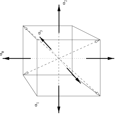
Figure 3. The $D(2|1;\alpha){}\rule[-20.0pt]{0.0pt}{20.0pt}$ root diagram.

can be visualised in a parallelipiped in 3d space with metric $g_{ij}=\mathrm{diag}(-1,-1,1)$. All odd roots are at the vertices of the parallelipiped on the light cone. Six even roots lie on the three lines through the centre of the faces. The Weyl group does not act transitively on the set of simple roots, and there are six choices of simple root systems.

We describe in more detail the system of simple roots with one odd root, $\alpha_{1}$, and two even roots, $\alpha_{2}$ and $\alpha_{3}$. The three regular $s\ell(2)$ subalgebras are in the directions of $\alpha_{2},\alpha_{3}$ and $\alpha_{\theta}=2\alpha_{1}+\alpha_{2}+\alpha_{3}$. The relevant scalar products are summarised as

(C.2) $$\alpha_{1}^{2}=0\,,\qquad\alpha_{2}^{2}=-2\gamma\,,\qquad\alpha_{3}^{2}=-2(1-\gamma)\,,\qquad\alpha_{\theta}^{2}=2\,,$$

(C.3) $$\alpha_{1}\cdot\alpha_{2}=\gamma\,,\qquad\alpha_{1}\cdot\alpha_{3}=1-\gamma\,,\qquad\alpha_{2}\cdot\alpha_{3}=0\,,$$

(C.4) $$\alpha_{3}\cdot\alpha_{\theta}=0\,,\qquad\alpha_{2}\cdot\alpha_{\theta}=0\,,\qquad\alpha_{1}\cdot\alpha_{\theta}=1,$$

where

(C.5) $$\gamma=\frac{\alpha}{1+\alpha},\qquad\gamma\in\mathbb{C}\setminus\{0,1,\infty\}.$$

With the metric above, we have

(C.6) $$\alpha_{1}=\tfrac{1}{\sqrt{2}}(-\sqrt{\gamma},-\sqrt{1-\gamma},1)\,,\qquad\alpha_{2}=(\sqrt{2\gamma},0,0)\,,\qquad\alpha_{3}=(0,\sqrt{2(1-\gamma)},0)\,.$$

The mapping $t_{1}:\gamma\mapsto 1-\gamma$ interchanges the rôles of $\alpha_{2}$ and $\alpha_{3}$, while the mapping $t_{2}:\gamma\mapsto\gamma^{-1}$ interchanges those of $\alpha_{2}$ and $\alpha_{\theta}$. These two transformations generate an order-6 group defined by the relations $t_{1}^{2}=t_{2}^{2}=1$, $t_{1}t_{2}t_{1}=t_{2}t_{1}t_{2}$, and one has the isomorphisms

(C.7) $$D(2|1;\tfrac{\gamma}{1-\gamma})\simeq{}D(2|1;\tfrac{1-\gamma}{\gamma})\simeq{}D(2|1;\tfrac{1}{\gamma-1})\simeq{}D(2|1;-\tfrac{1}{\gamma})\simeq{}D(2|1;\gamma-1)\simeq{}D(2|1;-\gamma).$$

If one restricts the parameter $\gamma$ to real values, it is sufficient to consider the domain $\gamma\in[1/2,1[$ for which $\alpha_{\theta}$ is always the longest root.

As far as the affine superalgebra is concerned, the isomorphisms are,

(C.8) $$\widehat{D}(2|1;\tfrac{\gamma}{1-\gamma})_{k}\simeq{}\widehat{D}(2|1;\tfrac{1-\gamma}{\gamma})_{k}\simeq{}\widehat{D}(2|1;\tfrac{1}{\gamma-1})_{-\frac{k}{\gamma}}\\ \simeq{}\widehat{D}(2|1;\gamma-1)_{-\frac{k}{\gamma}}\simeq{}\widehat{D}(2|1;-\tfrac{1}{\gamma})_{-\frac{k}{1-\gamma}}\simeq{}\widehat{D}(2|1;-\gamma)_{-\frac{k}{1-\gamma}}.$$

Appendix D $\widehat{s\ell}(2|1)$ OPE’s

We use a number of standard integrals, assuming whenever necessary that they are analytically continued from the domain where they are well-defined. For $\mathop{\mathsf{Re}}\nolimits z>\mathop{\mathsf{Re}}\nolimits w$, we have

(D.1) $$\int_{w}^{z}dx\,(z-x)^{\alpha}\,(x-w)^{\beta}=(z-w)^{a+b+1}\,\frac{\Gamma(\alpha+1)\Gamma(\beta+1)}{\Gamma(\alpha+\beta+2)}$$

and also

(D.2) $$\int_{z}^{\infty}dx\,(x-z)^{\alpha}\,(x-w)^{\beta}=(z-w)^{\alpha+\beta+1}\,\frac{\Gamma(\alpha+1)\Gamma(-1-\alpha-\beta)}{\Gamma(-\beta)}={}\\ {}=-(z-w)^{\alpha+\beta+1}\,\frac{\sin\pi\beta}{\sin\pi(\alpha+\beta)}\,\frac{\Gamma(\alpha+1)\Gamma(\beta+1)}{\Gamma(\alpha+\beta+2)}\,.$$

In evaluating the operator product $E^{1}(z)\cdot E^{2}(w)$, we have the following operators in (2.30): $V_{1}=e^{\frac{1}{\sqrt{2p}}\varphi}$, $V_{2}=e^{\frac{1}{\sqrt{2p}}\varphi}$, $V^{\prime}_{1}=e^{\frac{1}{\sqrt{2p^{\prime}}}\varphi^{\prime}}$, and $V^{\prime}_{2}=\gamma^{\prime}\,e^{\frac{1}{\sqrt{2p^{\prime}}}\varphi^{\prime}}$. Using the above integrals, we obtain

(D.3) $$\int_{z}^{\infty}\!\,du\,S(u)\,V_{1}(z)\,V_{2}(w)\int_{z}^{\infty}\!dx\,S^{\prime}(x)\,V^{\prime}_{1}(z)\,V^{\prime}_{2}(w)={}\\ {}=\beta(w)\,\frac{\sin\frac{\pi}{p}}{\sin\frac{2\pi}{p}}(z-w)^{\frac{1}{2p}+1-\frac{2}{p}}\frac{\Gamma(1-\frac{1}{p})\Gamma(1-\frac{1}{p})}{\Gamma(2-\frac{2}{p})}\cdot(z-w)^{\frac{1}{2p^{\prime}}-\frac{2}{p^{\prime}}}\frac{\Gamma(\frac{1}{p})\Gamma(2-\frac{2}{p})}{\Gamma(2-\frac{1}{p})}={}\\ {}=(z-w)^{-\frac{1}{2}}\beta(w)\,\frac{\pi p^{\prime}}{\sin\frac{2\pi}{p}}$$

plus lower-order terms. This is to be multiplied with the operator product  $e^{\frac{1}{\sqrt{2}}f(z)}\,e^{-\frac{1}{\sqrt{2}}f(w)}=(z-w)^{-\frac{1}{2}}+\dots$, which restores the first-order pole. We now recall the normalisation factors $(-1)\cdot\frac{i}{\pi p^{\prime}}\cos\frac{\pi}{p}$ from (2.12) and the factor $-2i\sin\tfrac{\pi}{p}$ from (2.30). This gives the operator product

$$\frac{-\beta(w)}{z-w}=\frac{E^{12}(w)}{z-w}\,,$$

which is in agreement with (B.1). The remaining terms in (2.30) cancel each other.

Evaluating the operator product $E^{1}(z)\cdot F^{1}(w)$, we have $V_{1}=e^{\frac{1}{\sqrt{2p}}\varphi}$, $V_{2}=\gamma\,e^{\frac{1}{\sqrt{2p}}\varphi}$, $V^{\prime}_{1}=e^{\frac{1}{\sqrt{2p^{\prime}}}\varphi^{\prime}}$, and $V^{\prime}_{2}=\gamma^{\prime}\,e^{\frac{1}{\sqrt{2p^{\prime}}}\varphi^{\prime}}$. Then

(D.4) $$\int_{z}^{\infty}du\,S(u)\,V_{1}(z)V_{2}(w)={}\\ {}=(z-w)^{\frac{1}{2p}}\int_{z}^{\infty}du\,(-\tfrac{1}{u-w}+\sqrt{\tfrac{2}{p}}\,\partial\varphi(w)+\beta\gamma(w)-\tfrac{1}{\sqrt{2p}}\,\partial\varphi(w)\,\tfrac{z-w}{u-w}+\dots)(u-z)^{-\frac{1}{p}}\,(u-w)^{-\frac{1}{p}}$$

(where the dots denote higher-order terms). This equals

(D.5) $${}=(z-w)^{\frac{1}{2p}-\frac{2}{p}}\,\frac{\Gamma(1-\frac{1}{p})\Gamma(-1+\frac{2}{p})}{\Gamma(\frac{1}{p})}\,\left(p-2+(z-w)\left(\sqrt{\tfrac{p}{2}}\,\partial\varphi(w)+\beta\gamma(w)\right)\right)\,.$$

Next, the primed sector integral $\int_{z}^{\infty}du\,S^{\prime}(u)\,V^{\prime}_{1}(z)V^{\prime}_{2}(w)$ is obtained from the last expression by simply replacing $p\mapsto p^{\prime}$, $\varphi\mapsto\varphi^{\prime}$, $\beta\mapsto\beta^{\prime}$, and $\gamma\mapsto\gamma^{\prime}$. Multiplying the primed and the unprimed contributions, we thus obtain

(D.6) $$\int_{z}^{\infty}\!\,du\,S(u)\,V_{1}(z)\,V_{2}(w)\int_{z}^{\infty}\!dx\,S^{\prime}(x)\,V^{\prime}_{1}(z)\,V^{\prime}_{2}(w)={}\\ {}=(z-w)^{\frac{1}{2}}\,\frac{\Gamma(1-\frac{1}{p})\Gamma(-1+\frac{2}{p})}{\Gamma(\frac{1}{p})}\,\biggl{(}\frac{p-2}{(z-w)^{2}}+\frac{\sqrt{\frac{p}{2}}\,\partial\varphi(w)+\beta\gamma(w)}{z-w}\biggr{)}\times{}\\ {}\times\frac{\Gamma(\frac{1}{p})\Gamma(1-\frac{2}{p})}{\Gamma(1-\frac{1}{p})}\,\biggl{(}\frac{p^{\prime}-2}{(z-w)^{2}}+\frac{\sqrt{\frac{p^{\prime}}{2}}\,\partial\varphi^{\prime}(w)+\beta^{\prime}\gamma^{\prime}(w)}{z-w}\biggr{)}={}\\ {}=(z-w)^{\frac{1}{2}}\,\frac{\pi}{\sin\frac{2\pi}{p}}\,\biggl{(}\frac{p^{\prime}(p-2)}{(z-w)^{2}}+\frac{p^{\prime}(\sqrt{\frac{p}{2}}\,\partial\varphi+\beta\gamma)-p(\sqrt{\frac{p^{\prime}}{2}}\,\partial\varphi^{\prime}+\beta^{\prime}\gamma^{\prime})}{z-w}\biggr{)}\,.$$

This is further multiplied with $e^{\frac{1}{\sqrt{2}}f(z)}\,e^{-\frac{1}{\sqrt{2}}f(w)}=(z-w)^{-\frac{1}{2}}(1+\frac{1}{\sqrt{2}}(z-w)\partial f+\dots)$; in addition, we recall the normalisations $(-1)\cdot\frac{i}{\pi p^{\prime}}\,\cos\frac{\pi}{p}$ in (2.12) and the factor $-2i\sin\tfrac{\pi}{p}$ from the first term in (2.30). Thus, the first term in (2.30) gives the contribution

(D.7) $$E^{1}(z)\,F^{1}(w)=\frac{-(p-2)}{(z-w)^{2}}+\frac{\frac{p}{p^{\prime}}(\sqrt{\frac{p^{\prime}}{2}}\,\partial\varphi^{\prime}+\beta^{\prime}\gamma^{\prime})-(\sqrt{\frac{p}{2}}\,\partial\varphi+\beta\gamma)-\frac{(p-2)}{\sqrt{2}}\partial f}{z-w}={}\\ {}=\frac{-k}{(z-w)^{2}}+\frac{H^{+}-H^{-}}{z-w}\,.$$

The remaining terms in (2.30) cancel each other and, therefore, the operator product $E^{1}(z)\,F^{1}(w)$ given by the last formula is in agreement with the respective commutator in (B.1).

We will need the first regular term in the above expansion when we calculate the $\widehat{s\ell}(2|1)$ energy-momentum tensor in Lemma 2.2, namely,

(D.8) $$-p^{\prime}E^{1}\,F^{1}=\tfrac{p^{\prime}}{\sqrt{2}}\beta\gamma\partial f-\tfrac{p}{\sqrt{2}}\beta^{\prime}\gamma^{\prime}\partial f-\sqrt{\tfrac{p}{2}}\,\beta^{\prime}\gamma^{\prime}\partial\varphi+\sqrt{\tfrac{p^{\prime}}{2}}\beta\gamma\partial\varphi^{\prime}-\sqrt{\tfrac{p(p-1)}{2}}\beta^{\prime}\gamma^{\prime}\partial\varphi^{\prime}\\ {}-\tfrac{\sqrt{p}}{\sqrt{2}(1-p)}\beta\gamma\partial\varphi{}+\tfrac{(p-2)\sqrt{p}}{2\sqrt{2}(p-1)}\partial^{2}\varphi+\tfrac{p+2}{4(p-1)}\partial\varphi\partial\varphi+\tfrac{(p-2)}{2\sqrt{2}}p^{\prime}\partial^{2}f-\tfrac{p-2}{2\sqrt{p-1}}\partial\varphi\partial\varphi^{\prime}\\ {}+\tfrac{1}{4}(2-3p)\partial\varphi^{\prime}\partial\varphi^{\prime}{}+\tfrac{p-2}{2}\sqrt{\tfrac{p^{\prime}}{2}}\partial^{2}\varphi^{\prime}+\tfrac{p^{\prime}}{2}\sqrt{p}\,\partial\varphi\partial f-\tfrac{p}{2}\sqrt{p^{\prime}}\partial\varphi^{\prime}\partial f+\tfrac{p^{\prime}}{4}\,(p-2)\partial f\partial f+\mathfrak{X}$$

where $\mathfrak{X}$ is a contribution that cancels against similar terms coming from $E^{2}\,F^{2}$.

As regards $E^{2}(z)\cdot F^{2}(w)$, we again use (2.30), where now $V_{1}=e^{\frac{1}{\sqrt{2p}}\varphi}$, $V_{2}=\gamma\,e^{\frac{1}{\sqrt{2p}}\varphi}$, $V^{\prime}_{1}=\gamma^{\prime}\,e^{\frac{1}{\sqrt{2p^{\prime}}}\varphi^{\prime}}$, and $V^{\prime}_{2}=e^{\frac{1}{\sqrt{2p^{\prime}}}\varphi^{\prime}}$. We already know from (D.5) the unprimed integral $\int_{z}^{\infty}du\,S(u)\,V_{1}(z)\,V_{2}(w)$; the primed sector contributes is evaluated similarly. We only quote the first regular term

(D.9) $$-p^{\prime}E^{2}\,F^{2}=-p\beta^{\prime}\partial\gamma^{\prime}-p^{\prime}\partial\beta\gamma+\sqrt{\tfrac{p^{\prime}}{2}}\beta\gamma\partial\varphi^{\prime}-\sqrt{\tfrac{p}{2}}\beta^{\prime}\gamma^{\prime}\partial\varphi+\tfrac{p^{\prime}}{\sqrt{2}}\beta\gamma\partial f+\tfrac{p}{\sqrt{2}}\beta^{\prime}\gamma^{\prime}\partial f\\ {}-\tfrac{\sqrt{p}}{\sqrt{2}(1-p)}\beta\gamma\partial\varphi-\sqrt{\tfrac{p(p-1)}{2}}\beta^{\prime}\gamma^{\prime}\partial\varphi^{\prime}+\tfrac{(p-2)p^{\prime}}{2\sqrt{2}}\partial^{2}f-\tfrac{p^{\prime}}{2}\sqrt{\tfrac{p}{2}}\partial^{2}\varphi-\tfrac{p}{2}\sqrt{\tfrac{p^{\prime}}{2}}\partial^{2}\varphi^{\prime}-\tfrac{p^{\prime}}{4}(p-2)\partial f\partial f\\ {}+\tfrac{p^{\prime}}{2}\sqrt{p}\,\partial\varphi\partial f+\tfrac{p}{2}\sqrt{p^{\prime}}\partial\varphi^{\prime}\partial f-\tfrac{p-2}{4(p-1)}\partial\varphi\partial\varphi+\tfrac{2-p}{2\sqrt{p-1}}\partial\varphi\partial\varphi^{\prime}+\tfrac{1}{4}(2-p)\partial\varphi^{\prime}\partial\varphi^{\prime}+\mathfrak{X}\,,$$

where $\mathfrak{X}$ is a contribution that cancels between $E^{1}\,F^{1}$ and $E^{2}\,F^{2}$.

The operator product $F^{1}(z)\cdot F^{2}(w)$ is evaluated similarly; we have $V_{1}=\gamma\,e^{\frac{1}{\sqrt{2p}}\varphi}$, $V_{2}=\gamma\,e^{\frac{1}{\sqrt{2p}}\varphi}$, $V^{\prime}_{1}=\gamma^{\prime}\,e^{\frac{1}{\sqrt{2p^{\prime}}}\varphi^{\prime}}$, and $V^{\prime}_{2}=e^{\frac{1}{\sqrt{2p^{\prime}}}\varphi^{\prime}}$. One then multiplies the contributions of the primed and unprimed sectors, given by

$$\int_{z}^{\infty}du\,S^{\prime}(u)\,V^{\prime}_{1}(z)\,V^{\prime}_{2}(w)=-(z-w)^{\frac{1}{2p^{\prime}}-\frac{2}{p^{\prime}}}\,\frac{\Gamma(-\frac{1}{p^{\prime}})\Gamma(\frac{2}{p^{\prime}})}{\Gamma(\frac{1}{p^{\prime}})}\,,$$

and

(D.10) $$\int_{z}^{\infty}du\,S(u)\,V_{1}(z)\,V_{2}(w)={}\\ {}=\int_{z}^{\infty}du\,\Bigl{(}\beta\gamma^{2}-\frac{\gamma(z)}{u-w}-\frac{\gamma(w)}{u-z}\Bigr{)}\Bigl{(}1-\sqrt{\tfrac{2}{p}}\,(u-w)\,\partial\varphi+\tfrac{1}{\sqrt{2p}}\,(z-w)\,\partial\varphi\Bigr{)}(u-z)^{-\frac{1}{p}}\,(u-w)^{-\frac{1}{p}}\\ {}=(z-w)^{\frac{1}{2p}-\frac{2}{p}+1}\,\frac{\Gamma(1-\frac{1}{p})\Gamma(-1+\frac{1}{p})}{\Gamma(\frac{1}{p})}\,(\beta\gamma^{2}+\sqrt{2p}\,\gamma\partial\varphi+(p-2)\partial\gamma)\,,$$

where we see the $J^{-}$ current from (2.22).

References

• [1] Aharony, G., Ganor, O., Sonnenschein, J., Yankielowicz, S., Sochen, N.: $G/G$ models and $W_{N}$ strings, Phys. Lett. B289, 309–316 (1992).
• [2] Bernard,Β D., Felder,Β G.: Fock Representations and BRST Cohomology inΒ s​ℓ^​(2)^𝑠ℓ2\widehat{s\ell}(2) Current Algebra, Commun. Math. Phys. 127 145–168 (1990).
• [3] Bershadsky,Β M., Lerche,Β W., Nemeschansky,Β D., and Warner,Β N.P.: Extended $N=2$ Superconformal Structure of Gravity and W Gravity Coupled to Matter, Nucl. Phys. B401 304–347 (1993).
• [4] Bershadsky, M., and Ooguri,Β H.: Hidden $Osp(N,2)$ Symmetries in Superconformal Field Theories, Phys. Lett. B229 374, (1989).
• [5] Bouwknegt,Β P., McCarthy,Β J., Pilch,Β K.: Quantum Group Structure in the Fock Space Resolutions ofΒ s​ℓ^​(n)^𝑠ℓ𝑛\widehat{s\ell}(n) Representations, Commun. Math. Phys. 131, 125–155 (1990).
• [6] Bouwknegt,Β P., McCarthy,Β J., Pilch,Β K.: Free-Field Approach to 2-Dimensional Conformal Field Theories, Prog. Theor. Phys. Suppl. 102, 67–135 (1990).
• [7] Bowcock,Β P., Hayes,Β M.R., Taormina,Β A.: Characters of admissible representations of the affine superalgebra $\widehat{s\ell}(2|1)$, Nucl. Phys. B510, 739–763 (1998).
• [8] Bowcock,Β P., Hayes,Β M.R., Taormina,Β A.: Parafermionic representation of the affine $\widehat{s\ell}(2|1)$ at fractional level, hep-th 9803024.
• [9] Bowcock,Β P., Koktava,Β R-L., Taormina,Β A.: Wakimoto modules for the affine superalgebra $\widehat{s\ell}(2|1)$ and noncritical $N=2$ strings, Phys. Lett. 388, 303–308 (1996).
• [10] Bowcock,Β P., Taormina,Β A.: Representation theory of the affine Lie superalgebra $\widehat{s\ell}(2|1)$ at fractional level, Commun. Math. Phys. 185, 467–493 (1997).
• [11] Cornwell,Β J.F.: Group Theory in Physics, Vol.3, Academic Press, 1989.
• [12] David,Β F.: Conformal field theories coupled to 2D-gravity in the conformal gauge, Mod. Phys. Lett. AΒ 3, 1651-1656 (1988).
• [13] Distler,Β J., Kawai,Β H.: Conformal field theory and 2D-quantum gravity, Nucl. Phys. B321, 509–527 (1989).
• [14] Fan,Β J-B., Yu,Β M.: Modules over affine Lie superalgebras, hep-th 9304122.
• [15] Fan,Β J-B., Yu,Β M.: $G/G$ gauged supergroup valued WZNW field theory, hep-th 9304123.
• [16] Feigin,Β B.L., Semikhatov,Β A.M, Sirota,Β V.Β A., and Tipunin,Β I.Yu.: Resolutions and Characters of Irreducible Representations of theΒ N=2𝑁2N=2 Superconformal Algebras, Nucl. Phys. B536 617–656 (1999).
• [17] Feigin,Β B.L., Semikhatov,Β A.M, and Tipunin,Β I.Yu.: Equivalence between Chain Categories of Representations of Affine $s\ell(2)$ and $N=2$ Superconformal Algebras, J.Β Math.Β Phys. 39 3865–3905 (1998).
• [18] Goddard,Β P., Olive,Β D.: Kac-Moody and Virasoro algebras in relation to quantum physics, Int. Jour.Β of Mod. Phys. A 303 (1986)
• [19] Gomez,Β C., Sierra,Β S.: The Quantum Symmetry of Rational Conformal Field Theories, Nucl. Phys. B352, 791–828 (1991)
• [20] Hayes,Β M.R., Taormina,Β A.: Admissible $\widehat{s\ell}(2|1)$ characters and parafermions, Nucl. Phys. B529, 588–610 (1998).
• [21] Hu,Β H.L.,Yu,Β M.: On the equivalence of non-critical strings and $G/G$ topological field theories, Phys. Lett. B 289, 302–308 (1992).
• [22] Ito,Β K., and Kanno,Β H.: Hamiltonian Reduction and Topological Conformal Algebra in $c\leq 1$ Non-Critical Strings, Mod. Phys. Lett. A9 1377 (1994).
• [23] Johnstone,Β G.B.: Modular Transformations and Invariants in the Context of Fractional Level $s\ell(2|1;C)$, in preparation.
• [24] Kač,Β V.G.: A sketch of Lie Superalgebra Theory, Commun. Math. Phys. 53, 31–64 (1977).
• [25] Kač,Β V.G.: Infinite Dimensional Lie Algebras, Cambridge University Press, 1990.
• [26] Kač,Β V.G., Peterson,Β D.H.: Infinite-dimensional Lie algebras, theta functions and modular forms, Adv.Β in Math. 53, 125–264 (1984).
• [27] Kač,Β V.G., Wakimoto M.: Modular invariant representations of infinite-dimensional Lie algebras and superalgebras, Proc. Nat. Acad. Sci. 85, 4956 (1988).
• [28] Kac,Β V. G., Wakimoto, M.: Integrable highest weight modules over affine superalgebras and number theory, hep-th 9407057.
• [29] Kassel,Β C.:Quantum Groups, Springer, 1995.
• [30] Mathieu,Β P., Walton,Β M.A.: On principal admissible representations and conformal field theory, hep-th 9812192.
• [31] Mukhi,Β S., Panda,Β S.: Fractional-Level Current Algebras and the Classification of Characters, Nucl. Phys. B338, 263–282 (1990).
• [32] Pressley,Β A., Segal,Β G.: Loop Groups, Oxford Mathematical Monographs, 1986.
• [33] Ramirez,Β C., Ruegg,Β H., RuizΒ Altaba,Β M.: Explicit Quantum Symmetries of WZNW Theories, Phys. Lett. B247, 499–508 (1990).
• [34] Semikhatov,Β A.M.: Verma Modules, Extremal Vectors, and Singular Vectors on the Non-Critical $N=2$ String Worldsheet, hep-th/9610084.
• [35] Semikhatov,Β A.M.: The Non-Critical $N=2$ String is an $s\ell(2|1)$ Theory, Nucl. Phys. B478, 209 (1996).
• [36] Tsuchiya,Β A., Kanie,Β Y.: Vertex Operators in the Conformal Field Theory on $\mathbb{P}^{1}$ and Monodromy Representations of the Braid Group, Lett. Math. Phys. 13, 303–312 (1987).