Abstract

It is argued that quantum traveling of D-particles presents the “joining-splitting” processes of field theory Feynman graphs. The amplitudes in $d$ dimensions can be corresponded with those of a $d+2$ dimensional theory in the Light-Cone frame. It is shown that this Light-Cone formulation enables to study processes with arbitrary longitudinal momentum transfers. It is discussed that a massless sector exists which can be taken as the low energy limit. By taking the constant relative distance in the bound-states we find a spectrum for the intermediatory fields.

Keywords: D-branes, M(atrix) Theories, Brane Dynamics in Gauge Theories

1 Introduction

Perturbative string theory is defined by series expansions based on the topologies of the string world-sheet, with the weights proportional to the action of string. The perturbation series can be presented as sum over different graphs which describe the “joining-splitting”(JS) processes of strings as events in space-time. In fact these graphs are those which should be obtained as Feynman graphs of a string field theory. In spite of the absence of a complete string field theory, those graphs which are produced by small strings ($\alpha^{\prime}\rightarrow 0$ limit) correspond to well known particle field theories namely various (super) gravity and gauge theories. So basically one expects to have a similar interpretation for JS processes of particles and corresponding particle field theory graphs.

On the other hand, through the developments of understanding of M-theory as a M(atrix) model [1], a description of perturbative Light-Cone string theory was achieved, based on a non-Abelian gauge theory living on a 2d cylinder which in most times can be interpreted as the world-sheet of free strings. This description was mentioned in [2, 3], more concreted in [4], and has been checked to produce the well known amplitudes in string theory [5, 6]. Besides in [7] (see also [8]) it was argued that configurations with different lengths of strings and their JS processes are corresponded to various backgrounds of world-sheet (gauge) fields. By the above picture for Feynman graphs of strings, it is the purpose of this letter to study similar ones for D-particles. It is argued that quantum traveling of D-particles are corresponded to graphs of a certain particle field theory and their amplitudes in the Light-Cone frame. So it provides the possibility of defining a particle field theory by its Feynman graphs, those generated by JS processes of D-particles.

It is useful to compare our approach to D-particle dynamics and that of M(atrix) model calculations [1]. In the case of M(atrix) model, because of large amount of supersymmetry, the D-particle action is trusted even for large separated D-particles; where it is not expected the action to be valid [9]. Though it may be taken an advantage, but lacks using the action in non-supersymmetric case. In our approach the dynamics of D-particles is used exactly in the region of kinematical variables where the action is defined. It causes that the calculation of D-particle scattering amplitudes can be performed even in the non-supersymmetric case. The gauge theoretic description of interactions in bosonic case is supported by the result of [5] for Light-Cone bosonic strings.

The organization of the article is as follows. In the next section we review some important aspects of D-particle dynamics. In section 3 the correspondence between D-particle quantum mechanics and the Light-Cone field theory amplitudes is presented. Section 4 is devoted to specification of the field theory in more details by estimating the masses of the intermediate states. Section 5 is for conclusion.

2 On D-Particles

D$p$-branes are $p$ dimensional objects which are defined as (hyper)surfaces which can trap the ends of strings [10]. One of the most interesting aspects of D-brane dynamics appears in their coincident limit. In the case of coinciding $N$ D$p$-branes, their dynamics are captured by dimensional reduction of $U(N)$ gauge theory to $p+1$ dimensions of D$p$-brane world-volume [11, 10].

For D-particles $(p=0)$ since only time exists in the world-line the above dynamics reduces to quantum mechanics of matrices. The bosonic action is [1, 12, 13]

$$S=m_{0}\int dt{\rm Tr}\;\biggl{(}{\frac{1}{2}}D_{t}X_{i}^{2}+\;\frac{1}{4(2\pi\alpha^{\prime})^{2}}\;[X_{i},X_{j}]^{2}\;\biggl{)},\;\;\;i=1,...,d,$$ (2.1)

where $\frac{1}{2\pi\alpha^{\prime}}$ and $m_{0}=(\sqrt{\alpha^{\prime}}g_{s})^{-1}$ are the string tension and the mass of D-particles respectively, and $g_{s}$ is string coupling. Here $D_{t}=\partial_{t}-iA_{0}$ acts as covariant derivative in the 0+1 dimensional gauge theory. For $N$ D-particles $X$’s are in adjoint representation of $U(N)$ and have the usual expansion $X_{i}=x_{ia}T_{a},\;\;a=1,...,N^{2}$, where $T_{a}$’s make basis of $U(N)$ algebra.

In fact this action is the result of the string theory calculation of D-brane interactions in the so-called gauge theory limit, defined by:

$$g_{s} \rightarrow 0,$$

$$l_{s} \rightarrow 0,$$

$$\frac{v}{l_{s}^{2}} = {\rm fixed},$$

$$\frac{r}{l_{s}^{2}} = {\rm fixed},$$ (2.2)

where $v$ and $r$ are the relative velocities and distances involved in the kinematics of D-branes and $l_{s}=\sqrt{\alpha^{\prime}}$ is the string length.

Firstly let us search for D-particles in the above Lagrangian:
For each direction $i$ there are $N^{2}$ variables instead of $N$ which one expects for $N$ particles. However there is a solution for the equations of motion which restricts the $T_{(a)}$ basis to the $N$ dimensional Cartan subalgebra. This solution causes vanishing the potential and one finds the equations of motion for $N$ free particles. In this case the $U(N)$ symmetry is broken to $U(1)^{N}$ and the interpretation of $N$ remaining variables as the classical relative positions of $N$ particles is meaningful. The center of mass of D-particles is represented by the trace of the $X$ matrices and easily can be seen that the momentum of the center of mass is conserved.

In the case of unbroken gauge symmetry the gauge transformations mix the entries of matrices and the interpretation of positions for D-particles remains obscure [14]. But even in this case the center of mass is meaningful and the ambiguity about positions only comes back to the relative positions of D-particles. In unbroken phase the $N^{2}-N$ non-Cartan elements of matrices have a stringy interpretation; they govern the dynamics of low lying oscillations of strings stretched between D-particles.

Let us study the limit $\alpha^{\prime}\rightarrow 0$ more carefully. Here this limit is analogous to the limit $g_{s}\rightarrow 0$ in [4]. In this limit to have a finite energy one has to restrict $X$’s to

$$[X_{i},X_{j}]=0,\;\;\;\forall\;i,j,$$ (2.3)

and consequently vanishing the potential term in the action. So the classical action reduces to the action of $N$ free particles

$$S=\int dt\sum_{a=1}^{N}{\frac{1}{2}}m_{0}\dot{x}_{a}^{2}.$$ (2.4)

However the above observation fails when D-particles arrive each other. When two D-particles come very near each other two eigenvalues of $X_{i}$ matrices will be equal and the corresponding off-diagonal elements can get non-zero values. This is the same story of gauge symmetry enhancement. The fluctuations of these off-diagonal elements are responsible for the interaction in D-particle bound-states.

In the non-coincident case we take simply the action (2.4). It is based on our expectation for free D-branes in large seperations [10]. For $N$ coincident D-particles one may write the action and Hamiltonian as,

$$S=\int dt\bigg{(}{\frac{1}{2}}(Nm_{0})\dot{X}^{2}+L_{int}(\hat{x}_{a},\dot{\hat{x}}_{a})\bigg{)},\;\;\;a=1,2,...,N^{2}-1,$$ (2.5)

$$H=\frac{P^{2}}{2(Nm_{0})}+H_{int}(\hat{x}_{a},\hat{p}_{a}),$$ (2.6)

in which $X$ and $P$ are the position and momentum of the center of mass and $\hat{x}_{a}$’s and $\hat{p}_{a}$’s are the non-Abelian positions and momenta.

The dependences of energy eigenvalues and the size of bound states are notable. By the scalings [12, 9]

$$t \rightarrow g_{s}^{-1/3}t,$$

$$A_{0} \rightarrow g_{s}^{1/3}A_{0},$$

$$X \rightarrow g_{s}^{1/3}X,$$ (2.7)

one finds the relevant energy and size scales as

$$E \sim g_{s}^{1/3}/l_{s},$$

$$l_{d+2} = g_{s}^{1/3}l_{s}.$$ (2.8)

The length scale $l_{d+2}$ should be the fundamental length scale of the covariant $d+2$ dimensional theory whose Light-Cone formulation is argued to be action (2.5) . In the weak coupling $g_{s}\to 0$ one finds $l_{d+2}\ll l_{s}$ which allows to treat the bound-states of finite number of D-particles as point like objects in the transverse dimensions of the Light-Cone frame. Also consequently one finds $m_{0}\cdot E\sim l_{d+2}^{-2}$ which shows invariance under boost transformation of this combination. As we will see the mass of the intermediate states appear as $\sim m_{0}\cdot E$.

3 D-Particle Feynman Graphs

Due to momentum conservation, $N$-particle states in Light-Cone frame have $NP_{+}$ longitudinal momentum. On the other hand, the longitudinal momentum of a state plays the role of the Newtonian mass in the transverse space of Light-Cone frame. So to have $N$-particle (normalizable) states the existence of marginal bound-states is necessary; those which are defined by $E_{binding}=0$. So the energy-mass equivalence relation for them is read as

$$E=M_{N}=N\cdot m_{0}$$ (3.1)

which in Light-Cone case we have $m_{0}=P_{+}$. The existence of normalizable marginal bound-states in D-particle case is clarified for supersymmetric case [16] , and also for bosonic case [17].

Here there are two possibilities to produce specified initial and final states, the so-called s- and t-channel processes.

s-channel

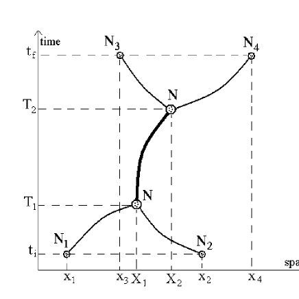
Figure 1: s-channel tree path for D-particles, $N=N_{1}+N_{2}=N_{3}+N_{4}$.

Take the probability amplitude corresponded to detect four clusters of D-particles, those with masses $N_{1}m_{0}$ and $N_{2}m_{0}$ in positions $x_{1}$ and $x_{2}$ at time $t_{i}$, and masses $N_{3}m_{0}$ and $N_{4}m_{0}$ in $x_{3}$ and $x_{4}$ at time $t_{f}$, presented by path integral as

$$\langle x_{3},x_{4};t_{f}|x_{1},x_{2};t_{i}\rangle=\int{\rm e}^{-S},$$ (3.2)

and supplied by the Newtonian mass conservation

$$N_{1}+N_{2}=N_{3}+N_{4}=N.$$ (3.3)

In the limit $\alpha^{\prime}\rightarrow 0$ one writes (Fig.1)

$$\langle x_{3},x_{4};t_{f}|x_{1},x_{2};t_{i}\rangle = \left[\int{\rm e}^{-S}\right]_{\alpha^{\prime}\rightarrow 0}$$ (3.4)

$$= \int_{t_{i}}^{t_{f}}dT_{1}dT_{2}\int_{-\infty}^{\infty}d^{d}X_{1}d^{d}X_{2}$$

$$\times \bigg{(}K_{N_{1}m_{0}}(X_{1},T_{1};x_{1},t_{i})K_{N_{2}m_{0}}(X_{1},T_{1};x_{2},t_{i})\bigg{)}$$

$$\times \bigg{(}K_{Nm_{0}}(X_{2},T_{2};X_{1},T_{1})K_{int}(\hat{x}_{2a}=0,T_{2};\hat{x}_{1a}=0,T_{1})\bigg{)}$$

$$\times \bigg{(}K_{N_{3}m_{0}}(x_{3},t_{f};X_{2},T_{2})K_{N_{4}m_{0}}(x_{4},t_{f};X_{2},T_{2})\bigg{)},$$

which $K_{m}(y_{2},t_{2};y_{1},t_{1})$ is the non-relativistic propagator of a free particle with mass $m$ between $(y_{1},t_{1})$ and $(y_{2},t_{2})$ , and $K_{int}$ is the corresponding propagator for the non-Abelian path integrations over $L_{int}(\hat{x}_{a},\dot{\hat{x}}_{a})$. In the above $\int dT_{1}dT_{2}dX_{1}dX_{2}$ is for a summation over different JS times and points. It is assumed that the group $U(1)\otimes SU(N_{1})\otimes SU(N_{2})$ for the position matrices is enhanced as $U(1)\otimes SU(N)$ at time $T_{1}$ and again is broken to $U(1)\otimes SU(N_{3})\otimes SU(N_{4})$ at time $T_{2}$.

We use the representations in $d$ dimensions

$$K_{m}(y_{2},t_{2};y_{1},t_{1}) = \theta(t_{2}-t_{1})\frac{1}{(2\pi)^{d}}\int d^{d}p\;{\rm exp}\bigg{(}ip\cdot(y_{2}-y_{1})-\frac{ip^{2}(t_{2}-t_{1})}{2m}\bigg{)},$$ (3.5)

$$K_{int}(\hat{x}_{2a},T_{2};\hat{x}_{1a},T_{1}) = \int d\hat{x}_{a}{\rm e}^{-S_{int}[T_{2},T_{1}]}=\sum_{n}\langle\hat{x}_{2a}|n\rangle\langle n|\hat{x}_{1a}\rangle{\rm e}^{-iE_{n}(T_{2}-T_{1})},$$ (3.6)

where $E_{n}$’s are the eigenvalues of $H_{int}$ of (2.6) and $\theta(t_{2}-t_{1})$ is the step function.

It is more convenient to translate every thing to the momentum space by ($E_{k}=\frac{p_{k}^{2}}{2N_{k}m_{0}}$, $k=1,2,3,4$)

$$\langle p_{3},p_{4},E_{3},E_{4};t_{f}|p_{1},p_{2},E_{1},E_{2};t_{i}\rangle \sim {\rm e}^{i(E_{3}+E_{4})t_{f}-i(E_{1}+E_{2})t_{i}}\int\prod_{k=1}^{4}d^{d}x_{k}\times$$ (3.7)

$${\rm e}^{i(p_{1}x_{1}+p_{2}x_{2}-p_{3}x_{3}-p_{4}x_{4})}\langle x_{3},x_{4};t_{f}|x_{1},x_{2};t_{i}\rangle,$$

and doing all integrations one finds (for $t_{i}=-\infty$ and $t_{f}=\infty$)

$$\langle p_{3},p_{4},E_{3},E_{4};\infty|p_{1},p_{2},E_{1},E_{2};-\infty\rangle \sim \delta^{(d)}(p_{1}+p_{2}-p_{3}-p_{4})\delta(E_{1}+E_{2}-E_{3}-E_{4})$$ (3.8)

$$\times\lim_{\epsilon\rightarrow 0^{+}}\sum_{n}\frac{i\langle\hat{x}_{2a}=0|n\rangle\langle n|\hat{x}_{1a}=0\rangle}{E-\frac{q^{2}}{2(Nm_{0})}-E_{n}+i\epsilon},$$

where $\vec{q}=\vec{p}_{1}+\vec{p}_{2}$ and $E=E_{1}+E_{2}$. Now recalling the energy-momentum relation in the Light-Cone frame for a particle with mass $M$

$$E\equiv q_{-}=\frac{{\vec{q}}^{2}+M^{2}}{2q_{+}},$$

one sees that the fraction in the sum of (3.8) is the the Light-Cone propagator of a particle [15] by identifications

$$q_{+} = Nm_{0},$$

$$M_{n}^{2} = 2Nm_{0}E_{n}.$$ (3.9)

The first relation of (3) learns us that each D-particle has Light-Cone momentum equal to $m_{0}$; this is because to have the Light-Cone momentum $Nm_{0}$ for $N$ D-particles in the time interval $[T_{1},T_{2}]$ (Fig.1). So (3.8) is the same expression which one writes (in momentum space) as tree diagram contribution to 4-point function of a field theory but in the Light-Cone frame [15], with exchanging masses as $M_{n}$’s. It is noted that $M_{n}^{2}\sim 1/l_{d+2}^{2}$.

In a covariant form one writes for (3.8)

$$\langle p_{3}^{\mu},p_{4}^{\mu};\infty|p_{1}^{\mu},p_{2}^{\mu};-\infty\rangle \sim \delta(\vec{p}_{1}+\vec{p}_{2}-\vec{p}_{3}-\vec{p}_{4})\delta(p_{-1}+p_{-2}-p_{-3}-p_{-4})$$ (3.10)

$$\times\lim_{\epsilon\rightarrow 0^{+}}\sum_{n}\frac{i2Nm_{0}\langle\hat{x}_{2a}=0|n\rangle\langle n|\hat{x}_{1a}=0\rangle}{q_{\mu}q^{\mu}-M_{n}^{2}+i\epsilon},$$

where $q^{\mu}=p_{1}^{\mu}+p_{2}^{\mu}$ and for any vector $V$ we have

$$V^{\mu}\equiv(\frac{V_{+}+V_{-}}{\sqrt{2}},\vec{V},\frac{V_{+}-V_{-}}{\sqrt{2}}),\;\mu=0,1,2,...,d,d+1.$$

So

$$p_{-k}\equiv\frac{\vec{p}_{k}^{2}}{2N_{k}m_{0}},\;\;\;p_{+k}\equiv N_{k}m_{0},\;\;k=1,2,3,4.$$

t-channel

The above considered amplitude for detecting four clusters of D-particles also can be studied in t-channel as (Fig.2)

$$\langle x_{3},x_{4};t_{f}|x_{1},x_{2};t_{i}\rangle = \left[\int{\rm e}^{-S}\right]_{\alpha^{\prime}\rightarrow 0}$$ (3.11)

$$= \int_{t_{i}}^{t_{f}}dT_{1}dT_{2}\int_{-\infty}^{\infty}d^{d}X_{1}d^{d}X_{2}$$

$$\times \bigg{(}K_{N_{1}m_{0}}(X_{1},T_{1};x_{1},t_{i})K_{N_{3}m_{0}}(x_{3},t_{f};X_{1},T_{1})\bigg{)}$$

$$\times \bigg{(}K_{N^{\prime}m_{0}}(X_{1},T_{1};X_{2},T_{2})K_{int}(\hat{x}_{2a}=0,T_{1};\hat{x}_{1a}=0,T_{2})\bigg{)}$$

$$\times \bigg{(}K_{N_{2}m_{0}}(X_{2},T_{2};x_{2},t_{i})K_{N_{4}m_{0}}(x_{4},t_{f};X_{2},T_{2})\bigg{)},$$

with the definitions mentioned earlier. In this channel as is specified in Fig.2, we have $T_{1}>T_{2}$. This is because of the unique direction of time in Light-Cone frame; see (3.5). So for every propagation of particles, e.g. intermediate states, propagations are from smaller time to bigger time.

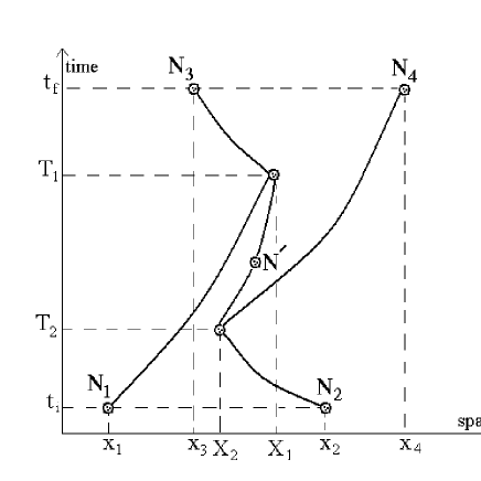
Figure 2: t-channel tree path for D-particles, $N^{\prime}=N_{2}-N_{4}=N_{3}-N_{1}$.

Again by going to the momentum space and doing all integrations one finds (for $t_{i}=-\infty$ and $t_{f}=\infty$)

$$\langle p_{3},p_{4},E_{3},E_{4};\infty|p_{1},p_{2},E_{1},E_{2};-\infty\rangle \sim \delta^{(d)}(p_{1}+p_{2}-p_{3}-p_{4})\delta(E_{1}+E_{2}-E_{3}-E_{4})$$ (3.12)

$$\times\lim_{\epsilon\rightarrow 0^{+}}\sum_{n}\frac{i\langle\hat{x}_{2a}=0|n\rangle\langle n|\hat{x}_{1a}=0\rangle}{(E_{3}-E_{1})-\frac{q^{\prime 2}}{2(N^{\prime}m_{0})}-E_{n}+i\epsilon},$$

where $\vec{{q^{\prime}}}=\vec{p}_{3}-\vec{p}_{1}$ and $N^{\prime}=N_{3}-N_{1}$. Again we have Light-Cone propagator of a particle [15] by identifications

$$q^{\prime}_{+} = N^{\prime}m_{0},$$

$$M_{n}^{2} = 2N^{\prime}m_{0}E_{n}.$$ (3.13)

In a covariant form one writes for (3.12)

$$\langle p_{3}^{\mu},p_{4}^{\mu};\infty|p_{1}^{\mu},p_{2}^{\mu};-\infty\rangle \sim \delta(\vec{p}_{1}+\vec{p}_{2}-\vec{p}_{3}-\vec{p}_{4})\delta(p_{-1}+p_{-2}-p_{-3}-p_{-4})$$ (3.14)

$$\times\lim_{\epsilon\rightarrow 0^{+}}\sum_{n}\frac{i2N^{\prime}m_{0}\langle\hat{x}_{2a}=0|n\rangle\langle n|\hat{x}_{1a}=0\rangle}{q^{\prime}_{\mu}q^{\prime\mu}-M_{n}^{2}+i\epsilon},$$

where $q^{\prime\mu}=p_{3}^{\mu}-p_{1}^{\mu}$.

4 Field Theory Of Feynman Graphs

The question of “what field theory?” is answered only by knowing the full set of eigenvalues and eigenvectors of the Hamiltonian $H_{int}$ defined by,

$$H_{int}|n\rangle=E_{n}|n\rangle.$$

The knowledge about the spectrum of the interested Hamiltonian is restricted. As is noted earlier the existence of zero-energy bound-states is discussed in [16, 17] . So, as the same of string theory, we have massless states which produce the low energy limit of the $d+2$ dimensional theory.

In the following we discuss another approach, the constant background.

4.1 Constant background

When two D-particles come very near each other two eigenvalues of $X_{i}$ matrices will become approximately equal and this makes the possibility that the corresponding off-diagonal elements take non-zero values.

In the coincident limit the dynamics is complicated. The relative matrix position may be taken as:

$$X_{i}=\left(\matrix{x_{i}&Y_{i}\cr Y_{i}^{*}&-x_{i}}\right),$$ (4.1)

where $Y^{*}$ is the complex conjugate of $Y$. By inserting this matrix in the Lagrangian one obtains:

$$S=\int dt{\frac{1}{2}}\bigg{(}(2m_{0})\dot{X_{i}}^{2}+m_{0}\dot{Y}_{i}\dot{Y}_{i}^{*}-m_{0}\frac{1}{4(2\pi\alpha^{\prime})^{2}}(1-\cos^{2}\theta)x_{j}^{2}Y_{i}Y_{i}^{*}+m_{0}\dot{x}_{j}^{2}+O(Y^{3})\bigg{)},$$ (4.2)

with $X$ for the center of mass and $\theta$ is the angle between $\vec{x}$ and the complex vector $\vec{Y}$. As is apparent in the limit $\alpha^{\prime}\rightarrow 0$ which is in our direct interest, the $x$ element can not get large values and have a small range of variation. In high-tension approximation of strings, one takes the relative distance of D-particles constant and of order of bound-state size $x\sim g_{s}^{1/3}l_{s}$, as was mentioned in Sec.2. So one writes:

$$S=\int dt\bigg{(}{\frac{1}{2}}(2m_{0})\dot{X_{i}}^{2}+{\frac{1}{2}}m_{0}\dot{Y}_{\perp}\cdot\dot{Y}_{\perp}^{*}-{\frac{1}{2}}m_{0}\frac{k^{2}g_{s}^{2/3}}{\alpha^{\prime}}Y_{\perp}\cdot Y_{\perp}^{*}+\cdot\cdot\cdot\bigg{)},$$ (4.3)

where in the above $k$ is an $\alpha^{\prime}$ independent numerical factor, and $Y_{\perp}$ is the perpendicular part of the $\vec{Y}$ to the relative distance $\vec{x}$. The parallel part of $\vec{Y}$ behaves as a free part. In $d+1$ dimensions of space-time the dimension of $Y_{\perp}$ is $d-1$ which shows that we are encountered with $2\times(d-1)$ harmonic oscillators because, $Y$ is a complex variable . These harmonic oscillators are corresponded to vibrations of oriented open strings stretched between D-particles.

By translating all the above to the momentum space and doing the integrals it is found

$$\langle p_{3},p_{4},E_{3},E_{4};t_{f}|p_{1},p_{2},E_{1},E_{2};t_{i}\rangle \sim \delta^{(d)}(p_{1}+p_{2}-p_{3}-p_{4})$$ (4.4)

$$\int_{t_{i}}^{t_{f}}dT_{1}dT_{2}\theta(T_{2}-T_{1})\times{\rm exp}(\frac{-i(p_{1}^{2}+p_{2}^{2})T_{1}}{2m_{0}})$$

$${\rm exp}(\frac{-iq^{2}(T_{2}-T_{1})}{4m_{0}}){\rm exp}(\frac{i(p_{3}^{2}+p_{4}^{2})T_{2}}{2m_{0}})$$

$$K_{oscillator}(Y_{\perp}=0,T_{2};Y_{\perp}=0,T_{1})$$

where $\vec{q}=\vec{p}_{1}+\vec{p}_{2}=\vec{p}_{3}+\vec{p}_{4}$, and

$$K_{oscillator}(Y_{\perp}=0,T_{2};Y_{\perp}=0,T_{1})=\theta(T_{2}-T_{1})\bigg{(}\frac{m_{0}\omega}{2\pi i\sin[\omega(T_{2}-T_{1})]}\bigg{)}^{d-1},$$

which $\omega$ is the harmonic oscillator frequency here to be $kg_{s}^{1/3}/l_{s}$. Since $Y_{\perp}$’s are complex numbers the power for the harmonic propagator is twice of $\frac{d-1}{2}$.

To have a real scattering process one assumes

$$t_{i}\rightarrow-\infty,\;\;\;t_{f}\rightarrow\infty.$$

We put $T\equiv T_{2}-T_{1}$ which has the range $0\leq T\leq\infty$. The integrals yield

$$\langle p_{3},p_{4};\infty|p_{1},p_{2};-\infty\rangle \sim \delta^{(d)}(p_{1}+p_{2}-p_{3}-p_{4})\delta(\frac{p_{1}^{2}}{2m_{0}}+\frac{p_{2}^{2}}{2m_{0}}-\frac{p_{3}^{2}}{2m_{0}}-\frac{p_{4}^{2}}{2m_{0}})$$ (4.5)

$$\int_{0}^{\infty}dT\;{\rm e}^{\frac{-iT}{4m_{0}}(q^{2}-2(p_{1}^{2}+p_{2}^{2}))}\bigg{(}\frac{m_{0}\omega}{\sin(\omega T)}\bigg{)}^{d-1},$$

By recalling the energy-momentum relation in the Light-Cone gauge one has:

$$2(p_{1}^{2}+p_{2}^{2})-q^{2}=2(2m_{0})(\frac{p_{1}^{2}+p_{2}^{2}}{2m_{0}})-q^{2}=2q_{+}q_{-}-q^{2}=q_{\mu}q^{\mu}\equiv q_{\mu}^{2}.$$

So it is found:

$$\langle p_{3},p_{4},E_{3},E_{4};\infty|p_{1},p_{2},E_{1},E_{2};-\infty\rangle \sim \delta^{(d)}(p_{1}+p_{2}-p_{3}-p_{4})\delta(E_{1}+E_{2}-E_{3}-E_{4})$$ (4.6)

$$\int_{0}^{\infty}dT{\rm e}^{\frac{-q_{\mu}^{2}}{4m_{0}}T}\bigg{(}\frac{m_{0}\omega}{\sin(\omega T)}\bigg{)}^{d-1}.$$

We perform a cut-off for $T$ in small values as $0<\epsilon\leq T\leq\infty$, with $\epsilon$ be small. By changing the integral variables as ${\rm e}^{-2\omega T}=\eta$ we have

$$\langle p_{3}^{\mu},p_{4}^{\mu};\infty|p_{1}^{\mu},p_{2}^{\mu};,-\infty\rangle \sim \delta^{(d)}(p_{1}+p_{2}-p_{3}-p_{4})\delta(p_{-1}+p_{-2}-p_{-3}-p_{-4})$$ (4.7)

$$\frac{(m_{0}\omega)^{d-1}}{2\omega}\int_{0}^{x}d\eta\;\eta^{\frac{-q_{\mu}^{2}}{8m_{0}\omega}+\frac{d-3}{2}}(1-\eta)^{-d+1},$$

$$\sim \delta^{(d)}(p_{1}+p_{2}-p_{3}-p_{4})\delta(p_{-1}+p_{-2}-p_{-3}-p_{-4})$$

$$\frac{(m_{0}\omega)^{d-1}}{2\omega}B_{x}(\frac{-q_{\mu}^{2}}{8m_{0}\omega}+\frac{d-1}{2},-d+2)$$

with $1\sim x={\rm e}^{-2\omega\epsilon}$ and $B_{x}$ is the Incomplete Beta function. It is recalled that the $m_{0}\omega$ is $1/l_{d+2}^{2}$. The longitudinal momentum conservation trivially is satisfied.

Polology

Equivalently one may use the other representation of $K_{oscillator}$ as

$$K_{oscillator}(Y_{\perp}=0,T_{2};Y_{\perp}=0,T_{1})=\sum_{n}\langle 0|n\rangle\langle n|0\rangle{\rm e}^{-iE_{n}(T_{2}-T_{1})},$$ (4.8)

with $E_{n}$’s as the known $H_{oscillator}$ eigenvalues. By this representation one finds the pole expansion :

$$\langle p_{3}^{\mu},p_{4}^{\mu};\infty|p_{1}^{\mu},p_{2}^{\mu};-\infty\rangle \sim \delta^{(d)}(p_{1}+p_{2}-p_{3}-p_{4})\delta(p_{-1}+p_{-2}-p_{-3}-p_{-4})$$ (4.9)

$$\times\lim_{\epsilon\rightarrow 0^{+}}\sum_{n}C_{n}\;\frac{i4m_{0}}{q_{\mu}q^{\mu}-M_{n}^{2}+i\epsilon}.$$

This pole expansion also can be derived by extracting the poles of the amplitude (4.7) with the condition

$$\frac{-q_{\mu}^{2}}{8m_{0}\omega}+\frac{d-1}{2}=-n,\;\;{\rm with}\;n\;{\rm as\;a\;positive\;integer}$$ (4.10)

or

$$M_{n}^{2}=\frac{8k(n+\frac{d-1}{2})}{l_{d+2}^{2}}.$$ (4.11)

5 Conclusion

It is argued in this work that the quantum mechanics of D-particles in $d$ dimensions can be corresponded to Light-Cone formulation of a $d+2$ dimensional field theory. The length scale of the $d+2$ dimensional theory is $g_{s}^{1/3}l_{s}$. Also it is shown that this Light-Cone formulation enables to study processes with arbitrary longitudinal momentum transfers. It is discussed that a massless sector exists which can be taken as the low energy limit of the $d+2$ dimensional theory. By taking the constant relative distances in the bound-states we found a spectrum for the intermediatory fields.

In the supersymmetric case a candidate for the $d+2$ dimensional theory can be guessed by M(atrix) theory approach to M-theory [1]. M-theory and type IIA string theory both have supergravities in their low energy limit in 11 and 10 dimensions respectively. There is a gauge theoretic description of stringy “Feynman Graphs” [2, 3, 4]. Since the 10 dimensional (IIA) supergravity is corresponded to stringy “Feynman Graphs” in the limit $\alpha^{\prime}\rightarrow 0$, so one may expect to have a similar relation between D-particles “Feynman Graphs” and 11 dimensional supergravity.

References

• [1] T. Banks, W. Fischler, S.H. Shenker and L. Susskind, Phys. Rev. D55 (1997) 5112, hep-th/9610043.
• [2] L. Motl, Proposals on Non-Perturbative Superstring Interactions, hep-th/9701025.
• [3] T. Banks and N. Seiberg, Nucl. Phys. B497 (1997) 41, hep-th/9702187.
• [4] R. Dijkgraaf, E. and H. Verlinde, Nucl. Phys. B500 (1997) 43, hep-th/9703030.
• [5] G.E. Arutyunov and S.A. Frolov, Theor. Math. Phys. 114 (1998) 43, hep-th/9708129.
• [6] G.E. Arutyunov and S.A. Frolov, Nucl. Phys. B524 (1998) 159, hep-th/9712061.
• [7] T. Wynter, Phys. Lett. 415B (1997) 349, hep-th/9709029.
• [8] S.B. Giddings, F. Hacquebord and H. Verlinde, Nucl. Phys. B537 (1999) 260, hep-th/9804121.
• [9] M.R. Douglas, D. Kabat, P. Pouliot and S.H. Shenker, Nucl Phys. B485 (1997) 85, hep-th/9608024.
• [10] J. Polchinski, Tasi Lectures on D-Branes, hep-th/9611050.
• [11] E. Witten, Nucl. Phys. B460 (1996) 335, hep-th/9510135.
• [12] D. Kabat and P. Pouliot, Phys. Rev. Lett. 77 (1996) 1004, hep-th/9603127;
U.H. Danielsson, G. Ferretti and B. Sundborg, Int. J. Mod. Phys. A11 (1996) 5463, hep-th/9603081.
• [13] M. Baake, P. Reinicke and V. Rittenberg, J. Math. Phys. 26 (1985) 1070;
R. Flume, Ann. Phys. 164 (1985) 189;
M. Claudson and M.B. Halpern, Nucl. Phys. B250 (1985) 689.
• [14] T. Banks, Matrix Theory, hep-th/9710231.
• [15] D. Bigatti and L. Susskind, Review of Matrix Theory, hep-th/9712072.
• [16] See for example: J. Frohlich, G.M. Graf, D. Hasler, J. Hoppe and S.-T. Yau, Asymptotic Form Of Zero Energy Wave Functions In Supersymmetric Matrix Model, hep-th/9904182, and references therein.
• [17] G. Gabadadze and Z. Kakushadze, Monopole Condensation, Matrix Quantum Mechanics and Membrane Approach in QCD, hep-th/9905198.
• [18] A.H. Fatollahi, Do Quarks Obey D-Brane Dynamics?, hep-ph/9902414.