Abstract

Using the AdS/CFT correspondence and the eikonal approximation, we evaluate the elastic parton-parton scattering amplitude at large $N$ and strong coupling $g_{YM}^{2}N$ in N=4 SYM. We obtain a scattering amplitude that reggeizes and unitarizes at large $\sqrt{s}$.

KIAS-P99045

1.   Elastic quark-quark and gluon-gluon scattering at large $s$ and fixed $t$ (Mandelstam variables) pertains to the domain of non-perturbative QCD. Theoretical procedures based on resuming large classes of perturbative contributions have been proposed [1, 2], partially accounting for the reggeized form of the scattering amplitude and the phenomenological success of pomeron/odderon exchange models [2] (and references therein). In an inspiring approach, Nachtmann [3] and others [4, 5, 6] suggested to use non-perturbative techniques for the elastic scattering amplitude. In the eikonal approximation and to leading order in $-t/s$ the quark-quark amplitude at large $s$ was reduced to a correlation function of two light-like Wilson-lines. The latter was assessed in the stochastic vacuum model [3].

Recently, Maldacena [7] has made the remarkable conjecture that the large $N$ behavior of $N=4$ supersymmetric gauge theory is dual to the string theory in a non-trivial geometry. This AdS/CFT conjecture, made more precise by Gubser, Klebanov and Polyakov [8] and by Witten [9] and extended to the non-supersymmetric case by Witten [10], provides an interesting and nonperturbative avenue for studying gauge theories at large $N$ and strong coupling $g_{YM}^{2}N$. In particular the heavy quark potential was found to be Coulombic for supersymmetric theories and linear for non-supersymmetric theories [9, 14].

In this letter we suggest to use the AdS/CFT approach to analyze the elastic parton-parton scattering amplitude in the eikonal approximation for $N=4$ SYM. In section 2 we briefly discuss the salient features of the parton-parton reduced elastic amplitude at large $\sqrt{s}$. The scattering amplitude in the eikonal approximation is reduced to the Fourier transform of the connected part of a correlator of two time-like Wilson lines. In section 3 we use the AdS/CFT approach to calculate the correlator. Following [11, 12], we propose that it is given by the minimum (regularized) area of the world-sheet with the time-like parton trajectories at its boundaries, and give a simple variational method that allows for a closed-form expression for the minimal area in the presence of a finite time cutoff. In section 4 we summarize and conclude.

2.   First consider the quark propagator in an external non-Abelian gauge field. In the first quantized theory, the propagator from $x$ to $y$ in Minkowski space reads

$${\bf S}(x,y;A)={\Big{<}}x|\frac{i}{i\hbox to0.0pt{/\hss}\nabla-m+i0}|y{\Big{>}}=\int_{0}^{\infty}dTe^{-i(m-i0)T}{\Big{<}}x|e^{-\hbox to0.0pt{/\hss}\nabla\,T}|y{\Big{>}}$$ (1)

that is [16, 17]

$${\bf S}(x,y;A)=\int_{0}^{\infty}\,dT\,e^{-i(m-i0)T}\,\int_{x}^{y}d[x]\,\,\delta(1-\dot{x}^{2})\,\,{\bf P}_{c}e^{ig_{YM}\int dsA\cdot\dot{x}}\,\,\frac{1}{2}{\bf P}_{s}e^{-\frac{i}{2}\int ds\,\sigma^{\mu\nu}\dot{x}_{\mu}\dot{\dot{x}}_{\nu}}$$ (2)

where ${\bf P}_{c,s}$ are orderings over color and spin matrices, and $\sigma_{\mu\nu}=[\gamma_{\mu},\gamma_{\nu}]/2$. The first exponent in the path integral is an arbitrary Wilson line in the fundamental representation of SU(N)_c, and the second exponent is a string of infinitesimal Thomas-precession along the Wilson line. The integration is over all paths with $x_{\mu}(0)=x_{\mu}$ and $x_{\mu}(T)=y_{\mu}$, where $T$ is the proper-time [17]. The dominant contributions come from those paths with $T\leq 1/m$. Heavy quarks travel shorter in proper-time than light quarks and the mass gives an effective cutoff of the proper-time range. This observation will be important below.

A quark with large momentum $p$ travels on a straight line with 4-velocity $\dot{x}_{\mu}=u_{\mu}=p_{\mu}/m$ and $u^{2}=1$. Throughout, we will distinguish between the 4-velocity $u_{\mu}$ and the instantaneous 3-velocity ${v}=dx/dt=p/E\leq 1$. For a straight trajectory, the 4-acceleration $\dot{\dot{x}}_{\mu}=a_{\mu}=0$ and the spin factor drops. This is the eikonal approximation for ${\bf S}$ in which an ordinary quark transmutes to a scalar quark. The present argument applies to any charged particle in a background gluon field, irrespective of its spin or helicity. The only amendments are: for antiquarks the 4-velocity $v_{\mu}$ is reversed in the Wilson line and the color matrices are in the complex representation, while for gluons the Wilson lines are in the adjoint representation. With this in mind, quark-quark scattering can be also extended to quark-antiquark, gluon-gluon or scalar-scalar scattering. We note that for quark-antiquark scattering the elastic amplitude dominates at large $\sqrt{s}$ since the annihilation part is down by $\sqrt{-t/s}$.

Generically, we will refer to elastic parton-parton scattering as

$$Q_{A}(p_{1})+Q_{B}(p_{2})\rightarrow Q_{C}(k_{1})+Q_{D}(k_{2})$$ (3)

with $s=(p_{1}+p_{2})^{2}$, $t=(p_{1}-k_{1})^{2}$, $s+t+u=4m^{2}$. We denote by $AB$ and $CD$ respectively, the incoming and outgoing color and spin of the quarks (polarization for gluons). Using the eikonal form for (1) and LSZ reduction, the scattering amplitude ${\cal T}$ may be reduced to [3, 4, 5]

$${\cal T}_{AB,CD}(s,t)\approx-2is\int d^{2}b\,\,e^{iq_{\perp}\cdot b}{\Big{<}}\left({\bf W}_{1}(b)\right)_{AC}\left({\bf W}_{2}(0)\right)_{BD}{\Big{>}}_{c}$$ (4)

where

$${\bf W}_{1,2}(z)={\bf P}_{c}{\rm exp}\left(ig_{YM}\int_{-\infty}^{+\infty}\,d\tau\,A(b+u_{1,2}\tau)\cdot u_{1,2}\right).$$ (5)

We are using the normalization $\left<{\bf W}\right>=1$, and retaining only the connected part in (4). The normalization can be relaxed if needed. The 2-dimensional integral in (4) is over the impact parameter $b$ with $t=-q_{\perp}^{2}$. In the CM frame $p_{1}\approx(E,E,0_{\perp})$, $p_{2}\approx(E,-E,0_{\perp})$, $q=p_{1}-k_{1}\approx(0,0,q_{\perp})$ and $s\approx 4E^{2}$. The averaging in (4) is over the gauge configurations using the QCD action. The total cross section for $\sqrt{s}>>\sqrt{-t}>0$ follows from (4) in the form $\sigma={Im\,\,{\cal T}}/s<{\rm ln}^{2}s$, where the last inequality is just the Froissart bound.

The amplitude (4) allows for two gauge-invariant decompositions (repeated indices are summed over)

$${\cal T}_{1}={\cal T}_{AB,AB}\qquad\qquad{\cal T}_{2}={\cal T}_{AB,BA}$$ (6)

assuming that the gluon-gauge fields are periodic at the end-points. We note that ${\cal T}_{2}$ is down by $1/N$ in comparison to ${\cal T}_{1}$. For gluon-gluon scattering the lines are doubled in color space (i.e., adjoint representation) and several gauge-invariant contractions are possible. For quark-quark scattering the singlet exchange in t-channel is 0⁺ (pomeron) while for quark-antiquark it is 0^- (odderon) as the two differ by charge conjugation.

3.   In the eikonal approximation the parton-parton scattering amplitude is related to an appropriate correlator of two Wilson lines. The typical duration of these light-like lines is $T\sim 1/m$ as we noted above. We now suggest to analyze the gauge-invariant correlators using the AdS/CFT [7, 9] approach for N=4 SYM.

The correlation function in large $N$ and strong coupling $g_{YM}^{2}N$ can be obtained from the minimal surface in the five-dimensional AdS space, [7, 12, 9] with the light-like Wilson lines at its boundaries as shown in Fig. 1.

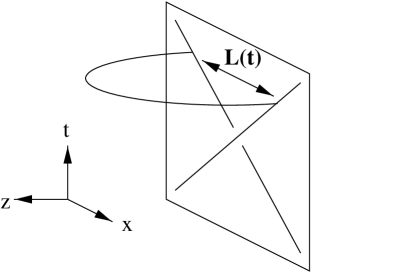
Figure 1: Wilson lines for moving partons with the attached AdS surface.

The classical action for a string world-sheet is

$$S=-\frac{1}{2\pi\alpha^{\prime}}\int d\xi d\sigma\sqrt{\det(G_{MN}\partial_{\alpha}X^{M}\partial_{\beta}X^{N})}.$$ (7)

The AdS metric $G_{MN}$ in Poincaré coordinates is given by

$$ds^{2}=R^{2}\frac{-dt^{2}+dx^{2}+dy^{2}+dw^{2}+dz^{2}}{z^{2}},$$ (8)

where $R=(2g^{2}_{YM}N\alpha^{\prime 2})^{1/4}$ is the radius of the AdS space, with $2\pi g_{st}=g_{YM}^{2}$. The AdS space has a boundary in Minkowski space $M_{4}$ at $z=0$. The boundary condition on the string world-sheet is given by the two time-like trajectories

$$x={v}t={u}\tau,y=0,z=0;\mbox{ and }\;x=-{v}t,y=b,z=0$$ (9)

with 3-velocities ${v}={u}/\gamma$ and $t$ the real time . The minimal surface associated to (7-9) leads to a set of coupled partial differential equations, which we have not yet managed to solve exactly. Instead, we provide a variational estimate as we now explain.

First, we divide the string world-sheet by constant time slices, each containing a string connected to two boundary points. Then we assume that for the minimal surface, this string length is minimal. So by finding the minimal length and carrying the integration over time, we will obtain an approximate minimal area. Specifically, we choose an orthogonal coordinate system $(\xi,\sigma)$ with the property $\partial_{\xi}X^{\mu}\partial_{\sigma}X^{\mu}=0$ on the world-sheet. Then,

$$S=-\frac{R^{2}}{2\pi\alpha^{\prime}}\int d\xi d\sigma\sqrt{(\partial_{\xi}X^{\mu})^{2}}\sqrt{\frac{(\partial_{\sigma}X^{\mu})^{2}}{z^{4}}}.$$ (10)

Let

$$l(t):=\int_{L(t)}d\sigma\sqrt{\frac{(\partial_{\sigma}x)^{2}+(\partial_{\sigma}y)^{2}+(\partial_{\sigma}w)^{2}+(\partial_{\sigma}z)^{2}}{z^{4}}}$$ (11)

be the ‘length’ of the string ending on the two receding quarks at the boundary with separation $L(t)$. $l(t)$ depends on $t$ only through $L(t)(=L(\tau))$, so that $l(t)$ and $l(\tau)$ represent the same quantity. First, we minimize this ‘length’ and then form the area by adding up the areas of the strips between the hyper-planes of time $t$ and $t+dt$. The height of the strip at the boundary is $dt\sqrt{1-{v}^{2}}=d\tau$ where $\tau$ is the proper-time at the boundary. The height of the strip at the central point of the string is given by $dt\sqrt{1-{\dot{z_{0}}(t)}^{2}}$ where ${z_{0}}(t)$ is the maximum value of $z$ at fixed $t$. Therefore by the trapezoidal rule, the minimal area is given by

$$A_{min}\simeq\frac{1}{2}\int dt\,\left(\sqrt{1-v^{2}}+\sqrt{1-{\dot{z_{0}}}^{2}}\right)\,l_{min}(t),$$ (12)

where $l_{min}(t)$ is the minimal length for a fixed time slice. To summarize: we have replaced $d\xi\sqrt{(\partial_{\xi}X^{\mu})^{2}}$ by $dt\,(\sqrt{1-v^{2}}+\sqrt{1-{\dot{z_{0}}}^{2}})/2$, which is $\sigma$ independent. The latter substitution is made in the CM frame. Lorentz invariance follows by rewriting the results in terms of Lorentz scalars.

The minimal length $l_{\min}(t)$ can be found by choosing a coordinate system such that the two quarks are located at $x=L(\tau)/2$ and $x=-L(\tau)/2$. Then

$$l(t)=\int_{-L(t)/2}^{+L(t)/2}dx\sqrt{\frac{1+z^{\prime 2}}{z^{4}}},$$ (13)

where $L(t)=\sqrt{b^{2}+4v^{2}t^{2}}$ (${u}\tau={v}t$) is the separation between the two time-like receding partons at the boundary $z=0$. In the instantaneous approximation, the string adjusts instantaneously to the change in the minimal length $L(t)$ at the boundary.  It follows that the problem of finding a minimal $l(t)$ is almost identical to the problem of finding a static $q{\bar{q}}$ potential [11, 12]. The result for a properly regularized length is

$$l(t)=-\frac{c_{0}}{L(t)}$$ (14)

with $c_{0}=(2\pi)^{3}/\Gamma(\frac{1}{4})^{4}$ and ${z_{0}}(t)$ given by

$${z_{0}}(t)=c_{1}L(t),$$ (15)

where $c_{1}=1/\sqrt{c_{0}}\simeq 0.834$. Hence under the instantaneous approximation, the ‘area’ is obtained by integrating the static potential.

$$A_{min} \simeq -\frac{1}{2}\int_{-T}^{T}dt\,\left(\sqrt{1-v^{2}}+\sqrt{1-{\dot{z_{0}}}^{2}}\right)\,\frac{c_{0}}{\sqrt{b^{2}+4{v}^{2}t^{2}}}$$ (16)

$$= -\left(\sqrt{1-v^{2}}+\sqrt{1-(2c_{1}{v})^{2}}\right)\frac{c_{0}}{2{v}}\sinh^{-1}\left(\frac{2{v}T}{b}\right).$$

According to the AdS/CFT correspondence [9, 11], the connected part of the Wilson-line correlator in N=4 SYM at large $N$ and fixed $g_{YM}^{2}N$ is

$${\Big{<}}{\bf WW}{\Big{>}}_{c}\approx\exp(iS)=\exp\left[ic_{0}\sqrt{2g_{YM}^{2}N}\left(\sqrt{1-v^{2}}+\sqrt{1-(2c_{1}{v})^{2}}\right)\frac{1}{2{v}}\ln\left(\frac{4{v}T}{b}\right)\right].$$ (17)

This result may be contrasted with the one-gluon exchange contribution to the connected and untraced correlator (dropping color factors)

$${\Big{<}}{\bf WW}{\Big{>}}_{1c}\approx-\frac{g_{YM}^{2}}{4\pi^{2}}\,\int_{-\infty}^{+\infty}d\tau_{1}d\tau_{2}\frac{u_{1}\cdot u_{2}}{\left(-(u_{1}\tau_{1}-u_{2}\tau_{2})^{2}+b^{2}\right)}=i\frac{g_{YM}^{2}}{4\pi}\left(v+\frac{1}{v}\right)\,{\rm ln}\left(\frac{T}{b}\right).$$ (18)

The natural infrared cutoff in the problem is the mass; $T=1/\mu\sim 1/m$. For quarks and gluons, it is simply their constituent mass. In QED, (18) exponentiates with a noticeable difference from (17) : the time dilatation factors generated by the string are absent in QED. This very difference will cause the scattering amplitude to reggeize in our case instead of eikonalize as we will show below.

To restore Lorentz invariance, we can rewrite eq.(17) in terms of the Mandelstam variable $s$,

$${\Big{<}}{\bf WW}{\Big{>}}_{c} \approx \left(\frac{4\sqrt{1-4m^{2}/s}}{\mu b}\right)^{ic_{0}\sqrt{2g_{YM}^{2}N}\left(\frac{m}{\sqrt{s-4m^{2}}}+\frac{1}{2}\sqrt{\frac{s}{s-4m^{2}}-(2c_{1})^{2}}\right)}$$ (19)

where we have made the substitutions : ${u}=\sqrt{\frac{s}{4m^{2}}-1}$, ${v}=\sqrt{1-\frac{4m^{2}}{s}}$ and $T=1/\mu$ for the time cutoff. At this stage, several remarks are in order.

• Notice that $\sqrt{1-(2c_{1}{v})^{2}}$ is purely imaginary for ${v}>1/2c_{1}\simeq 0.6$, resulting in a suppression of the scattering amplitude at large $\sqrt{s}$. This happens because the central part of the string moves into the AdS space with a velocity $\sim 2c_{1}v>1$, which is classically forbidden by the 5 dimensional kinematics. This is a flaw of the instantaneous approximation we discussed above, that can be ultimately resolved by an analytical or numerical investigation of the exact solution to the minimal surface problem. Here, we observe that this pathology can be removed by physical arguments on the CFT side. Indeed, from (19) we note that the pathological behavior of the string yields a new branch-point singularity in the s-channel, besides the expected free threshold at $s=4m^{2}$. In a non-confining and conformally invariant SYM theory, this is unphysical. This singularity disappears if and only if $2c_{1}$ is renormalized to 1. This means that the exact treatment of the minimal surface should yield a result where the maximum speed of the central point of the string is 1, in accordance with relativity. When this happens,

  $${\Big{<}}{\bf WW}{\Big{>}}_{c} \approx \left(\frac{4\sqrt{1-4m^{2}/s}}{m\mu b}\right)^{ic_{0}\sqrt{2g_{YM}^{2}N}\left(\frac{2m}{\sqrt{s-4m^{2}}}\right)}$$ (20)

• Eq.(16) might be interpreted to suggest using the proper-time $d\tau=\sqrt{1-v^{2}}dt$ instead of the global varaible $t$ in the final stage of the calculation. It is important to realize that if the $fixed$ time cutoff $T=1/{\mu}$ was substituted by a $fixed$ proper time cutoff then the result would be (20) with the substitution $1/\mu\rightarrow\sqrt{s}/2m\mu$. The former ($t$) is favored by the string theory calculation of the minimal surface and to compare the well-known eikonal form in the Abelian case such as QED [5, 19] as well as the result of the perturbative calculation eq.(18). The latter($\tau$) is favored by manifest Lorentz invariance and the representation (1-2). The situation is such that string theory calculation with time cutoff gives the gaugy theory results with formalism using the proper-time. Fortunately, whether we use the proper-time or time cutoff, both lead to the same scattering amplitude asymptotically (see below). Note that the elastic amplitude involves typically momenta of order $\sqrt{-t}$, so that $b\sim 1/\sqrt{-t}$. As a result, the ‘cross singularity’ of the two Wilson loops at $b=0$ [5] is dynamically regulated for fixed Mandelstam variable $t$.

• The Minkowski AdS/CFT approach followed here is subtle. For example, the concept of a minimum surface is not well defined in a metric with indefinite signature. A more rigorous treatment is to setup the problem in a metric with an Euclidean signature and then perform a Wick-rotation of the outcome. We have checked that our present answer is unchanged by this procedure. The factor $i$ in the exponent of (20) follows from $1/v_{E}$ ($v_{E}={dx}/{d\,t_{E}},it=t_{E}$), which is real with an Euclidean signature but imaginary with a Minkowski signature.

Using (20), the gauge-invariant combination of the parton-parton scattering amplitude (6) now reads

$${\cal T}(s,t)\approx 4\pi\alpha(s)\frac{\Gamma(1-i\alpha(s))}{\Gamma(1+i\alpha(s))}\left(\frac{2s}{-t}\right)\,\left(\frac{2\sqrt{-t}}{\mu}\right)^{2i\alpha(s)}$$ (21)

for large $N$ and fixed $g_{YM}^{2}N$. Here the gamma functions come from $2\pi\int_{0}^{\infty}db^{\prime}b^{\prime 1-2i\alpha(s)}J_{0}(b^{\prime})$ with $\alpha(s)$ given by

$$\alpha(s)={c_{0}\sqrt{2g_{YM}^{2}N}\left[\frac{m}{\sqrt{s-4m^{2}}}\right]}.$$ (22)

A similar behavior follows from a proper time cutoff through the substitution $1/\mu\rightarrow\sqrt{s}/2m\mu$. The result (21) is reminiscent of the QED result [19], but with important differences. The amplitude has a nonperturbative dependence on $g_{YM}^{2}N$, much like the static potential [11, 12]. The amplitude reggeizes and unitarizes at large $\sqrt{s}$. Indeed, asymptotically ($s>>-t,m^{2}$)

$${\cal T}(s,t)\approx 4\pi c_{0}\sqrt{2g^{2}_{YM}N}\left(\frac{2s}{-t}\right)\,\left(\frac{s}{m^{2}}\right)^{-0.5}$$ (23)

which is real (no inelasticity), independent of the cutoff $\mu$, and with a negative intercept of $-0.5$. The zero imaginary part and the nonzero intercept are both tied to the the occurrence of a string in the AdS space as is explicit from (17). On the boundary, the receding partons with momenta $\sqrt{s}$ define a range in rapidity space of the order of ${\rm ln}\,s$. Powers of ${\rm ln}\,s$ count the number of ‘gluons’ exchanged in the t-channel. Since (23) can be written as a power series in ${\rm ln}\,s$, it contains terms with an infinite number of gluon exchange. A similar observation was also made by Verlinde and Verlinde [4] in the process of mapping high-energy scattering onto a two-dimensional sigma model.

Finally, the present arguments also show that at large $N$ and strong $g_{YM}^{2}N$, the cross sections for quark-quark and quark-antiquark scattering are the same. The gluon-gluon scattering amplitude could be calculated similarly with the substitution $N\rightarrow N^{2}$, due to the adjoint representation of the gluon.

4.   We have presented arguments for evaluating the elastic parton-parton scattering amplitude at large $N$ and strong $g_{YM}^{2}N$ in N=4 SYM. Although the latter is conformally invariant in $M_{4}$ the appearance of the string picture and the necessity to regulate the elastic contribution in time has led to a reggeized behavior that unitarizes at large $\sqrt{s}$. The result cannot be reached by perturbation theory. The nature of the result depends sensitively on the string character of the underlying description and hence is not applicable to Abelian-like theories such as QED.

Our main result follows from a physically motivated variational estimate of the minimal surface in the AdS space. The exact form of the extremal surface is too involved to be written down analytically. Although an exact result would of course be ideal, we do not expect our estimate of the parton-parton cross section to change appreciably. Indeed, the dominant contributions arise from scattering with large impact parameter $b\sim 1/\sqrt{-t}$, for which our approximation for the extremal surface should be legitimate. For a large impact parameter $b$, the extremal surface is smoothly twisted and the eikonal approximation is also good.

Finally and from a different standpoint, Verlinde and Verlinde [4] have shown that at large $\sqrt{s}$ the elastic amplitudes in QCD follows from a two-dimensional sigma model with conformal symmetry, where the latter is broken when the light-like quark lines are regulated in the time-like direction. Does the large $N$ effective action derived by Verlinde and Verlinde [4] map onto an AdS type action? Is there a way to do better than the variational estimate made in the present analysis? How could we recover the true Regge behavior of non-supersymmetric QCD? Some of these questions will be addressed in a forthcoming publication.

Acknowledgments We wish to thank KIAS for their generous hospitality and support during this work. We are grateful to Kyungsik Kang, Taekoon Lee, Maciek Nowak and Martin Rocek for discussions, and Romuald Janik for comments on the manuscript. We are especially thankful to Igor Klebanov for comments and helpful suggestions. The work of IZ was supported in part by US-DOE grant DE-FG-88ER40388 and that of SJS by the program BSRI-98-2441.

Note Added

After posting our paper, [20] appeared in which a similar approach is suggested for scattering between colorless states at large impact parameters.

References

- [1] L.N. Lipatov, Perturbative QCD, ed. A.H. Mueller (World Scientific, Singapore, 1989), and references therein.
- [2] G. Sterman, hep-ph/9905548, and references therein.
- [3] O. Nachtmann, Ann. Phys. 209 (1991) 436; hep-ph/9609365.
- [4] H. Verlinde and E. Verlinde, hep-ph/9302104.
- [5] G.P. Korchemsky, Phys. Lett. B 325 (1994) 459.
- [6] I.Ya. Aref’eva, Phys. Lett. B325 (1994) 171, hep-th/9311115.
- [7] J. Maldacena, Adv. Theor. Math. Phys. 2 (1998) 231, hep-th/9711200.
- [8] S.S. Gubser, I.R. Klebanov and A.M. Polyakov, Phys. Lett. B428 (1998) 105.
- [9] E. Witten, Adv. Theor. Math. Phys. 2 (1998) 253, hep-th/9802150.
- [10] E. Witten, Adv. Theor. Math. Phys. 2 (1998) 505, hep-th/9803131.
- [11] J. Maldacena, Phys. Rev. Lett. 80 (1998) 4859.
- [12] Soo-Jong Rey and Jung-Tay Yee, hep-th/9803001.
- [13] Soo-Jong Rey, Stefan Theisen and Jung-Tay Yee, Nucl. Phys. B527 (1998) 171, hep-th/9803135.
- [14] A. Brandhuber, N. Itzhaki, J. Sonnenschein and S. Yankielowicz, JHEP 9806 (1998) 001, hep-th/9803263.
- [15] A. Brandhuber, N. Itzhaki, J. Sonnenschein and S. Yankielowicz, Phys. Lett. B434 (1998) 36.
- [16] A. Strominger, Phys. Lett. B101 (1981) 271; M. Nowak, M. Rho and I. Zahed, Phys. Lett. B254 (1991) 94.
- [17] A.M. Polyakov, Gauge Fields and Strings, Harwood 1987.
- [18] E. Witten, In “Recent developments in gauge theories”, ed. G. ’t Hooft et.al, Plenum, NY 1980; O. Haas, Phys. Lett. B106 (1981) 207.
- [19] H. Cheng and T. Wu, Phys. Rev. Lett. 22 (1969) 666; H. Abarbanel and C. Itzykson, Phys. Rev. Lett. 23 (1969) 53.
- [20] R.A. Janik and R. Peschanski, hep-th/9907177.