FTUAM-99/22

IASSNS-HEP-99/62

IFT-UAM/CSIC-99-26

hep-th/9907086

Orientifolding the conifold
J. Park^†, R. Rabadán^§ and A. M. Uranga^†
† School of Natural Sciences, Institute for Advanced Study,
Olden Lane, Princeton NJ 08540, USA
^§ Departamento de Física Teórica C-XI and Instituto de Física Teórica C-XVI,
Universidad Autónoma de Madrid, Cantoblanco, 28049 Madrid, Spain
Abstract

In this paper we study the ${\cal N}=1$ supersymmetric field theories realized on the world-volume of type IIB D3-branes sitting at orientifolds of non-orbifold singularities (conifold and generalizations). Several chiral models belong to this family of theories. These field theories have a T-dual realization in terms of type IIA configurations of relatively rotated NS fivebranes, D4-branes and orientifold six-planes, with a compact $x^{6}$ direction, along which the D4-branes have finite extent. We compute the spectrum on the D3-branes directly in the type IIB picture and match the resulting field theories with those obtained in the type IIA setup, thus providing a non-trivial check of this T-duality. Since the usual techniques to compute the spectrum of the model and check the cancellation of tadpoles, cannot be applied to the case orientifolds of non-orbifold singularities, we use a different approach, and construct the models by partially blowing-up orientifolds of $\bf C^{3}/(\bf Z_{2}\times\bf Z_{2})$ and $\bf C^{3}/(\bf Z_{2}\times\bf Z_{3})$ orbifolds.

1 Introduction

The recent developments in the study of supersymmetric field theories by embedding them into string theory has profited from the interplay of different approaches. The most relevant ones for our purposes in this paper are the realization in terms of D-branes in the presence of NS-branes (and possibly other higher-dimensional D-branes) [1, 2, 3, 4], and in terms of D-branes probes at spacetime singularities [5, 6]. These two broad classes of constructions are related by T-dualities [7, 8, 9, 10], which transform the NS-fivebranes into geometric singularities [11]. This type of mapping allows to answer different questions in the different pictures. Thus, the brane configurations of NS-branes and D-branes are very intuitive and allow to easily classify large classes of models and their corresponding field theories. On the other hand, the picture of branes at singularities contains only perturbative objects and is better suited for some explicit computations of perturbative effects in the corresponding field theory, for instance anomaly cancellation conditions and one-loop beta functions [12, 13]. Also, the large N limit of the field theory can be studied in term of a dual supergravity (or superstring) background by means of the AdS/CFT correspondence [14].

In this paper we are going to consider type IIA configurations of NS-fivebranes (with world-volume along the directions 012345), NS^′-branes (along 012389), with D4-branes (along 01236) suspended between them, and in the presence of D6^′-branes and O6^′-planes (both along 0123457). These constructions realize a variety of four-dimensional ${\cal N}=1$ supersymmetric gauge field theories on the D4-brane world-volume. Configurations of this type, but without orientifold planes, were first introduced in [2]. The introductions of orientifold planes was discussed in [15, 16, 17] (see also [18, 19]).

We will be interested in configurations where the direction $x^{6}$, along which the D4-branes are suspended between the NS fivebranes, is compactified on a circle. Our basic aim is to understand the resulting configurations after performing a T-duality along this direction. There are basically two motivations for this. The first is that the IIB T-dual picture provides an interesting insight into several non-trivial brane dynamics effects that occur on the type IIA side, and which are related to chiral symmetries and chiral matter in the gauge field theory. These include the appearance of chiral symmetries and chiral flavours when a half-D6^′ brane ends on a NS-brane [20], the appearance of chiral matter due to the change of sign of the O6^′-plane charge when it crosses a NS-brane [15, 16, 17]. The type IIB realization of these effects has been studied in [21] (some had been previously observed in [22]) in the simpler case where NS^′-branes are absent . This paper can be regarded as an extension of these result to more general models.

The second and maybe more interesting motivation is that the T-dual configurations involve orientifolds of non-orbifold singularities. This can be seen as follows. Type IIA configurations of $k$ NS-branes, $k^{\prime}$ NS^′-branes and D4-branes, without orientifold planes, but with compact direction $x^{6}$, transform under T-duality into a set of D3-branes probing the non-orbifold singularity $xy=z^{k^{\prime}}{w}^{k}$ [9] (see also [10] for the particular case $k=k^{\prime}=1$). Therefore, it is reasonable to expect the IIA models with O6^′-planes to correspond to suitable orientifolds of these non-orbifold spaces. In this paper we would like to construct such orientifolds directly on the IIB side and compare the resulting field theories on the D3-brane probes with those obtained in the IIA setup. Unfortunately, this problem is rather difficult, since the usual techniques to construct type IIB orientifolds, compute the field theory spectrum and check the cancellation of twisted RR tadpoles (and ensure the consistency of the string theory configurations) [23, 24, 25, 26, 27, 28] do not apply, since the world-sheet description of these models is not a solvable conformal field theory. On the other hand, this means that the type IIA configurations can provide, through the T-duality, interesting information about the possible consistent orientifolds of non-orbifold spaces. In this paper, however, we will construct the IIB models directly and use the results as new support for the T-duality proposal.

The procedure we use is based in the observation in [29] that one can construct non-orbifold singularities as partial resolutions of orbifold singularities. The effect of the blow-ups appears in the D3-brane field theory as specific Higgs breakings which can be identified in a precise manner. The effective field theory along the Higgs branch gives the field theory of the D3-branes at the non-orbifold singularity. We apply this idea in the presence of an additional orientifold projection; that is, we study partial resolutions of orientifolds of orbifold singularities to construct orientifolds of non-orbifold singularities. Due to the complexity of the method (concretely, the identification of the Higgsing associated to a specific blow-up) we will mainly discuss the simplest examples with at most three NS fivebranes. Some comments about more general cases are mentioned at the end.

As mentioned above, the singularity realization of these field theories provides a simple description of several exotic phenomena in the IIA side. This point was already stressed in the simplest context of [21], so we will not insist on it here. Another interesting observation suggested by our constructions is that the chiral theories obtained in the IIA framework (and other related ${\cal N}=1$ models) are continuously connected to other chiral theories obtained by orientifolding orbifold singularities. The relation is the process of blowing-up of the singularity probed by the D3-branes, or equivalently the Higgs breaking in the field theory. We find this picture quite reassuring, and satisfactory, since it suggests a unified description for all chiral gauge theories which can be embedded in string theory.

The paper is organized as follows. In Section 2 we review the field theories arising from type IIA configurations with NS-branes, NS^′-branes and D4-branes, with the direction 6 compact, but without orientifold planes. We also review the T-duality with sets of D3-branes at non-orbifold singularities. As a preparation for analogous computations in the orientifolded case, we review the construction in [29] of the field theories on D3-branes at the conifold ($xy=zw$) and suspended pinch point ($xy=zw^{2}$) singularities, by blowing up the $\bf C^{3}/(\bf Z_{2}\times\bf Z_{2})$ orbifold singularity. The techniques of toric geometry required for these computations have been confined to section 2.2.1, so that it can be (hopefully) safely avoided by readers not interested in them.

In Section 3 we turn to the type IIA configurations including O6^′-planes. As explained above, we center on the simplest examples, with one NS-brane and one NS^′-brane (which T-dualize to orientifolds of the conifold), or one NS-brane and two NS^′-branes (which T-dualize to orientifolds of the suspended pinch point).

The type IIB orientifolds of the suspended pinch point, $xy=zw^{2}$, are the subject of Section 4. They can be obtained as partial resolutions of suitable orientifolds of $\bf C^{3}/(\bf Z_{2}\times\bf Z_{2})$. These are constructed in Section 4.1, where we also check explicitly the cancellation of tadpoles. In Section 4.2 we discuss the blow-ups which provide the orientifolds of $xy=zw^{2}$, and the associated field theory Higgsings. The resulting field theories match nicely those obtained from the type IIA constructions. We also comment on some interesting results obtained upon continuing blowing-up.

In Section 5 we discuss orientifolds of the conifold. These cannot be obtained by resolving orientifolds of $\bf C^{3}/(\bf Z_{2}\times\bf Z_{2})$, since the orientifold projection eliminates the required blow-up mode. However, they can be constructed by resolving orientifolds of $\bf C^{3}/(\bf Z_{2}\times\bf Z_{3})$ . We describe the highlights of the computations involved, and describe the results. The field theories obtained after the Higgsing again reproduce those obtained from the IIA side.

Finally, in Section 6 we make several remarks concerning the generalization of our results to arbitrary singularities $xy=z^{k}w^{k^{\prime}}$ (T-duals of models with $k$ NS-branes and $k^{\prime}$ NS^′-branes, and end with some final comments.

2 Rotated branes and non-orbifold singularities

We start with a brief review of some simple IIA brane configurations, and their IIB T-dual version as D3-branes at singularities, before the introduction of orientifold projections.

2.1 ${\cal N}=1$ elliptic models

There is a natural way to break the ${\cal N}=2$ supersymmetry of the elliptic models considered in [30] to ${\cal N}=1$, namely to use NS-fivebranes whose world-volumes are relatively rotated. In this paper we will consider only fivebranes with worldvolume along 012345 (denoted NS-branes) and along 012389 (denoted NS^′-branes). Thus we restrict to fivebranes which are either parallel or orthogonal, even when more general angles are allowed. This type of configurations was first considered in [2] (see [3] for further references) in models with non-compact $x^{6}$. We will be interested in models with $x^{6}$ compact, which were discussed in [9, 31]. We will refer to them as ${\cal N}=1$ elliptic models.

It is straightforward to read off the resulting ${\cal N}=1$ field theories. For a model with $k$ NS-branes and $l$ NS^′-branes, we obtain a gauge group $\prod_{i=1}^{k+l}SU(n_{i})$ (times a decoupled $U(1)$, ignored in the following), and bifundamental chiral multiplets $\sum_{i=1}^{k+l}\,[\,(\raisebox{-0.5pt}{\hbox{\rule{0.4pt}{6.5pt}\hskip-0.4pt\rule{6.5pt}{0.4pt}\hskip-6.5pt\rule[6.5pt]{6.5pt}{0.4pt}}\rule[6.5pt]{0.4pt}{0.4pt}\hskip-0.4pt\rule{0.4pt}{6.5pt}}_{i},\overline{\raisebox{-0.5pt}{\hbox{\rule{0.4pt}{6.5pt}\hskip-0.4pt\rule{6.5pt}{0.4pt}\hskip-6.5pt\rule[6.5pt]{6.5pt}{0.4pt}}\rule[6.5pt]{0.4pt}{0.4pt}\hskip-0.4pt\rule{0.4pt}{6.5pt}}}_{i+1})+(\overline{\raisebox{-0.5pt}{\hbox{\rule{0.4pt}{6.5pt}\hskip-0.4pt\rule{6.5pt}{0.4pt}\hskip-6.5pt\rule[6.5pt]{6.5pt}{0.4pt}}\rule[6.5pt]{0.4pt}{0.4pt}\hskip-0.4pt\rule{0.4pt}{6.5pt}}}_{i},\raisebox{-0.5pt}{\hbox{\rule{0.4pt}{6.5pt}\hskip-0.4pt\rule{6.5pt}{0.4pt}\hskip-6.5pt\rule[6.5pt]{6.5pt}{0.4pt}}\rule[6.5pt]{0.4pt}{0.4pt}\hskip-0.4pt\rule{0.4pt}{6.5pt}}_{i+1})\,]$. We also get a massless adjoint whenever two adjacent fivebranes are parallel, which parametrizes a Coulomb branch in which D4-branes slide along the NS-branes. When two adjacent fivebranes are orthogonal, there is quartic superpotential for the bifundamental fields living at the ends of the interval (see [9] for more details).

In [9] (and in [10] in a particular case) it was argued that a T-duality along $x^{6}$ maps this configuration to a system of D3-branes at a non-orbifold singularity $xy=z^{l}w^{k}$. The result follows from the T-duality between a NS fivebrane and a Taub-NUT space $xy=v$ [11]. In the general case, the singularity requires additional data to specify the field theory completely. In particular, the different orderings of NS and NS^′ branes in $x^{6}$ corresponds to a specific choice of B-fields in the collapsed two-cycles in the singularity. This subtlety will not arise in the particular models we study.

Figure 1: Examples of ${\cal N}=1$ elliptic models. Figure a) is T-dual to a set of D3-branes at a conifold singularity $xy=zw$. Figure b) is T-dual to D3-branes at the ‘suspended pinch point’ singularity, $xy=zw^{2}$.

The main examples we will consider are depicted in figure 1. The first configuration, figure 1a, contains one NS brane and one NS^′ brane. It realizes a field theory with the following gauge group and ${\cal N}=1$ matter content

$$\begin{array}[]{cccc}&SU(n_{1})&SU(n_{2})&\\ A_{i}&\raisebox{-0.5pt}{\hbox{\rule{0.4pt}{6.5pt}\hskip-0.4pt\rule{6.5pt}{0.4pt}\hskip-6.5pt\rule[6.5pt]{6.5pt}{0.4pt}}\rule[6.5pt]{0.4pt}{0.4pt}\hskip-0.4pt\rule{0.4pt}{6.5pt}}&\overline{\raisebox{-0.5pt}{\hbox{\rule{0.4pt}{6.5pt}\hskip-0.4pt\rule{6.5pt}{0.4pt}\hskip-6.5pt\rule[6.5pt]{6.5pt}{0.4pt}}\rule[6.5pt]{0.4pt}{0.4pt}\hskip-0.4pt\rule{0.4pt}{6.5pt}}}&i=1,2\\ B_{i}&\overline{\raisebox{-0.5pt}{\hbox{\rule{0.4pt}{6.5pt}\hskip-0.4pt\rule{6.5pt}{0.4pt}\hskip-6.5pt\rule[6.5pt]{6.5pt}{0.4pt}}\rule[6.5pt]{0.4pt}{0.4pt}\hskip-0.4pt\rule{0.4pt}{6.5pt}}}&\raisebox{-0.5pt}{\hbox{\rule{0.4pt}{6.5pt}\hskip-0.4pt\rule{6.5pt}{0.4pt}\hskip-6.5pt\rule[6.5pt]{6.5pt}{0.4pt}}\rule[6.5pt]{0.4pt}{0.4pt}\hskip-0.4pt\rule{0.4pt}{6.5pt}}&i=1,2\end{array}$$ (2.4)

The superpotential is given by

$$W = {\rm Tr\,}(A_{1}B_{1}A_{2}B_{2}-A_{1}B_{2}A_{2}B_{1}).$$ (2.5)

After T-dualizing along $x^{6}$ this configuration maps to a set of D3 branes at a conifold singularity $xy=zw$. In fact, the above field theory was proposed in [32] to arise on D3-branes at the conifold singularity, on the basis of strong evidence from the AdS/CFT correspondence.

The second configuration, figure 1b, contains one NS-brane and two NS^′-branes. The corresponding gauge group and matter content are

$$\begin{array}[]{cccc}&SU(n_{1})&SU(n_{2})&SU(n_{3})\\ F&\raisebox{-0.5pt}{\hbox{\rule{0.4pt}{6.5pt}\hskip-0.4pt\rule{6.5pt}{0.4pt}\hskip-6.5pt\rule[6.5pt]{6.5pt}{0.4pt}}\rule[6.5pt]{0.4pt}{0.4pt}\hskip-0.4pt\rule{0.4pt}{6.5pt}}&\overline{\raisebox{-0.5pt}{\hbox{\rule{0.4pt}{6.5pt}\hskip-0.4pt\rule{6.5pt}{0.4pt}\hskip-6.5pt\rule[6.5pt]{6.5pt}{0.4pt}}\rule[6.5pt]{0.4pt}{0.4pt}\hskip-0.4pt\rule{0.4pt}{6.5pt}}}&\\ {\tilde{F}}&\overline{\raisebox{-0.5pt}{\hbox{\rule{0.4pt}{6.5pt}\hskip-0.4pt\rule{6.5pt}{0.4pt}\hskip-6.5pt\rule[6.5pt]{6.5pt}{0.4pt}}\rule[6.5pt]{0.4pt}{0.4pt}\hskip-0.4pt\rule{0.4pt}{6.5pt}}}&\raisebox{-0.5pt}{\hbox{\rule{0.4pt}{6.5pt}\hskip-0.4pt\rule{6.5pt}{0.4pt}\hskip-6.5pt\rule[6.5pt]{6.5pt}{0.4pt}}\rule[6.5pt]{0.4pt}{0.4pt}\hskip-0.4pt\rule{0.4pt}{6.5pt}}&\\ G&&\raisebox{-0.5pt}{\hbox{\rule{0.4pt}{6.5pt}\hskip-0.4pt\rule{6.5pt}{0.4pt}\hskip-6.5pt\rule[6.5pt]{6.5pt}{0.4pt}}\rule[6.5pt]{0.4pt}{0.4pt}\hskip-0.4pt\rule{0.4pt}{6.5pt}}&\overline{\raisebox{-0.5pt}{\hbox{\rule{0.4pt}{6.5pt}\hskip-0.4pt\rule{6.5pt}{0.4pt}\hskip-6.5pt\rule[6.5pt]{6.5pt}{0.4pt}}\rule[6.5pt]{0.4pt}{0.4pt}\hskip-0.4pt\rule{0.4pt}{6.5pt}}}\\ {\tilde{G}}&&\overline{\raisebox{-0.5pt}{\hbox{\rule{0.4pt}{6.5pt}\hskip-0.4pt\rule{6.5pt}{0.4pt}\hskip-6.5pt\rule[6.5pt]{6.5pt}{0.4pt}}\rule[6.5pt]{0.4pt}{0.4pt}\hskip-0.4pt\rule{0.4pt}{6.5pt}}}&\raisebox{-0.5pt}{\hbox{\rule{0.4pt}{6.5pt}\hskip-0.4pt\rule{6.5pt}{0.4pt}\hskip-6.5pt\rule[6.5pt]{6.5pt}{0.4pt}}\rule[6.5pt]{0.4pt}{0.4pt}\hskip-0.4pt\rule{0.4pt}{6.5pt}}\\ H&\overline{\raisebox{-0.5pt}{\hbox{\rule{0.4pt}{6.5pt}\hskip-0.4pt\rule{6.5pt}{0.4pt}\hskip-6.5pt\rule[6.5pt]{6.5pt}{0.4pt}}\rule[6.5pt]{0.4pt}{0.4pt}\hskip-0.4pt\rule{0.4pt}{6.5pt}}}&&\raisebox{-0.5pt}{\hbox{\rule{0.4pt}{6.5pt}\hskip-0.4pt\rule{6.5pt}{0.4pt}\hskip-6.5pt\rule[6.5pt]{6.5pt}{0.4pt}}\rule[6.5pt]{0.4pt}{0.4pt}\hskip-0.4pt\rule{0.4pt}{6.5pt}}\\ {\tilde{H}}&\raisebox{-0.5pt}{\hbox{\rule{0.4pt}{6.5pt}\hskip-0.4pt\rule{6.5pt}{0.4pt}\hskip-6.5pt\rule[6.5pt]{6.5pt}{0.4pt}}\rule[6.5pt]{0.4pt}{0.4pt}\hskip-0.4pt\rule{0.4pt}{6.5pt}}&&\overline{\raisebox{-0.5pt}{\hbox{\rule{0.4pt}{6.5pt}\hskip-0.4pt\rule{6.5pt}{0.4pt}\hskip-6.5pt\rule[6.5pt]{6.5pt}{0.4pt}}\rule[6.5pt]{0.4pt}{0.4pt}\hskip-0.4pt\rule{0.4pt}{6.5pt}}}\\ \Phi_{1}&{\rm Adj.}&&\end{array}$$ (2.14)

The superpotential is given by

$$W = {\rm tr\,}({\tilde{F}}FG{\tilde{G}}-{\tilde{G}}GH{\tilde{H}}+{\tilde{H}}H\Phi_{1}-{\tilde{F}}\Phi_{1}F).$$ (2.15)

After T-duality, this configuration transforms into a set of D3 branes at the so-called ‘suspended pinch point’ (SPP) singularity, $xy=zw^{2}$. This T-duality is supported by the fact that independent arguments [29] (to be reviewed in the following section) imply that the above field theory is indeed realized on D3-branes at the SPP singularity.

It is rather difficult to study D3-branes at non-orbifold singularities, the reason being that they are not described by free world-sheet conformal field theories. From this point of view it is fortunate that for toric singularities there exists a systematic (though involved) approach, based on [6] and developed in [29], that allows to compute the spectrum and interactions of the D3-brane field theory. Therefore, before entering the study of the orientifold models, which are more complicated, it will be convenient to review the description of the conifold and SPP models using these techniques.

2.2 Non-orbifold singularities from orbifold singularities

The main observation is that the non-orbifold singularities of interest, the conifold $xy=zw$ and the SPP $xy=zw^{2}$, can be constructed as partial resolutions of the $\bf C^{3}/(\bf Z_{2}\times\bf Z_{2})$ orbifold singularity. The latter is obtained upon modding out the $\bf C^{3}$ parametrized by $(z_{1},z_{2},z_{3})$ by the group generated by

$$\theta: (z_{1},z_{2},z_{3})\rightarrow(-z_{1},z_{2},-z_{3})$$

$$\omega: (z_{1},z_{2},z_{3})\rightarrow(z_{1},-z_{2},-z_{3})$$ (2.16)

Defining invariant variables, $x=z_{1}^{2}$, $y=z_{2}^{2}$, $z=z_{3}^{2}$, $w=z_{1}z_{2}z_{3}$, the space can be describe as the hypersurface

$$xyz=w^{2}$$ (2.17)

in $\bf C^{4}$. This space can be blown-up once by introducing a ${\rm I\kern-1.79993ptP}_{1}$ parametrized by $w^{\prime}=w/z$ (in the coordinate patch $z\neq 0$). The remaining singularity has the form

$$xy=zw^{\prime}{\,{}^{2}}$$ (2.18)

which is a suspended pinch point singularity. There are two inequivalent ways of performing a further blow-up. The first possibility is to introduce a ${\rm I\kern-1.79993ptP}_{1}$ parametrized e.g. by $x^{\prime}=x/w^{\prime}$. The remaining singularity is the conifold $x^{\prime}y=zw^{\prime}$. The second possibility is to introduce a ${\rm I\kern-1.79993ptP}_{1}$ parametrized e.g. by $y^{\prime}=y/z$. The remaining singularity is $xy^{\prime}=w^{\prime 2}$, the $\bf C^{2}/\bf Z_{2}\times\bf C$ orbifold. For any of these two possibilities further blow-ups yield a completely smooth space.

Our aim in this section is to construct the field theory of D3-branes at these non-orbifold singularities by starting with the well-known system of D3-branes at $\bf C^{3}/(\bf Z_{2}\times\bf Z_{2})$ and following the effect of the above blow-ups in the field theory.

The field theory of a set of D3-branes at a $\bf C^{3}/(\bf Z_{2}\times\bf Z_{2})$ singularity can be easily constructed following [6]. We mod out a system of D3 branes in flat space by the action (2.16), embedded on the D3-brane Chan-Paton factors through the matrices

$$\gamma_{\theta,3}={\rm diag\,}(1_{n_{1}},1_{n_{2}},-1_{n_{3}},-1_{n_{4}})$$

$$\gamma_{\omega,3}={\rm diag\,}(1_{n_{1}},-1_{n_{2}},1_{n_{3}},-1_{n_{4}})$$ (2.19)

The resulting field theory is found by imposing the projections

$$\begin{array}[]{cccc}V=\gamma_{\theta,3}V\gamma_{\theta,3}^{-1}\;,&X=-\gamma_{\theta,3}X\gamma_{\theta,3}^{-1}\;,&Y=\gamma_{\theta,3}Y\gamma_{\theta,3}^{-1}\;,&Z=-\gamma_{\theta,3}Z\gamma_{\theta,3}^{-1}\\ V=\gamma_{\omega,3}V\gamma_{\omega,3}^{-1}\;,&X=\gamma_{\omega,3}X\gamma_{\omega,3}^{-1}\;,&Y=-\gamma_{\omega,3}Y\gamma_{\omega,3}^{-1}\;,&Z=-\gamma_{\omega,3}Z\gamma_{\omega,3}^{-1}\end{array}$$ (2.22)

The gauge group is $U(n_{1})$$\times U(n_{2})$$\times U(n_{3})$$\times U(n_{4})$, and there are ${\cal N}=1$ matter multiplets

$$X_{13}:(\raisebox{-0.5pt}{\hbox{\rule{0.4pt}{6.5pt}\hskip-0.4pt\rule{6.5pt}{0.4pt}\hskip-6.5pt\rule[6.5pt]{6.5pt}{0.4pt}}\rule[6.5pt]{0.4pt}{0.4pt}\hskip-0.4pt\rule{0.4pt}{6.5pt}}_{1},\overline{\raisebox{-0.5pt}{\hbox{\rule{0.4pt}{6.5pt}\hskip-0.4pt\rule{6.5pt}{0.4pt}\hskip-6.5pt\rule[6.5pt]{6.5pt}{0.4pt}}\rule[6.5pt]{0.4pt}{0.4pt}\hskip-0.4pt\rule{0.4pt}{6.5pt}}}_{3}) \quad Y_{12}:(\raisebox{-0.5pt}{\hbox{\rule{0.4pt}{6.5pt}\hskip-0.4pt\rule{6.5pt}{0.4pt}\hskip-6.5pt\rule[6.5pt]{6.5pt}{0.4pt}}\rule[6.5pt]{0.4pt}{0.4pt}\hskip-0.4pt\rule{0.4pt}{6.5pt}}_{1},\overline{\raisebox{-0.5pt}{\hbox{\rule{0.4pt}{6.5pt}\hskip-0.4pt\rule{6.5pt}{0.4pt}\hskip-6.5pt\rule[6.5pt]{6.5pt}{0.4pt}}\rule[6.5pt]{0.4pt}{0.4pt}\hskip-0.4pt\rule{0.4pt}{6.5pt}}}_{2}) \quad Z_{14}:(\raisebox{-0.5pt}{\hbox{\rule{0.4pt}{6.5pt}\hskip-0.4pt\rule{6.5pt}{0.4pt}\hskip-6.5pt\rule[6.5pt]{6.5pt}{0.4pt}}\rule[6.5pt]{0.4pt}{0.4pt}\hskip-0.4pt\rule{0.4pt}{6.5pt}}_{1},\overline{\raisebox{-0.5pt}{\hbox{\rule{0.4pt}{6.5pt}\hskip-0.4pt\rule{6.5pt}{0.4pt}\hskip-6.5pt\rule[6.5pt]{6.5pt}{0.4pt}}\rule[6.5pt]{0.4pt}{0.4pt}\hskip-0.4pt\rule{0.4pt}{6.5pt}}}_{4})$$

$$X_{31}:(\raisebox{-0.5pt}{\hbox{\rule{0.4pt}{6.5pt}\hskip-0.4pt\rule{6.5pt}{0.4pt}\hskip-6.5pt\rule[6.5pt]{6.5pt}{0.4pt}}\rule[6.5pt]{0.4pt}{0.4pt}\hskip-0.4pt\rule{0.4pt}{6.5pt}}_{3},\overline{\raisebox{-0.5pt}{\hbox{\rule{0.4pt}{6.5pt}\hskip-0.4pt\rule{6.5pt}{0.4pt}\hskip-6.5pt\rule[6.5pt]{6.5pt}{0.4pt}}\rule[6.5pt]{0.4pt}{0.4pt}\hskip-0.4pt\rule{0.4pt}{6.5pt}}}_{1}) \quad Y_{21}:(\raisebox{-0.5pt}{\hbox{\rule{0.4pt}{6.5pt}\hskip-0.4pt\rule{6.5pt}{0.4pt}\hskip-6.5pt\rule[6.5pt]{6.5pt}{0.4pt}}\rule[6.5pt]{0.4pt}{0.4pt}\hskip-0.4pt\rule{0.4pt}{6.5pt}}_{2},\overline{\raisebox{-0.5pt}{\hbox{\rule{0.4pt}{6.5pt}\hskip-0.4pt\rule{6.5pt}{0.4pt}\hskip-6.5pt\rule[6.5pt]{6.5pt}{0.4pt}}\rule[6.5pt]{0.4pt}{0.4pt}\hskip-0.4pt\rule{0.4pt}{6.5pt}}}_{1}) \quad Z_{41}:(\raisebox{-0.5pt}{\hbox{\rule{0.4pt}{6.5pt}\hskip-0.4pt\rule{6.5pt}{0.4pt}\hskip-6.5pt\rule[6.5pt]{6.5pt}{0.4pt}}\rule[6.5pt]{0.4pt}{0.4pt}\hskip-0.4pt\rule{0.4pt}{6.5pt}}_{4},\overline{\raisebox{-0.5pt}{\hbox{\rule{0.4pt}{6.5pt}\hskip-0.4pt\rule{6.5pt}{0.4pt}\hskip-6.5pt\rule[6.5pt]{6.5pt}{0.4pt}}\rule[6.5pt]{0.4pt}{0.4pt}\hskip-0.4pt\rule{0.4pt}{6.5pt}}}_{1})$$

$$X_{24}:(\raisebox{-0.5pt}{\hbox{\rule{0.4pt}{6.5pt}\hskip-0.4pt\rule{6.5pt}{0.4pt}\hskip-6.5pt\rule[6.5pt]{6.5pt}{0.4pt}}\rule[6.5pt]{0.4pt}{0.4pt}\hskip-0.4pt\rule{0.4pt}{6.5pt}}_{2},\overline{\raisebox{-0.5pt}{\hbox{\rule{0.4pt}{6.5pt}\hskip-0.4pt\rule{6.5pt}{0.4pt}\hskip-6.5pt\rule[6.5pt]{6.5pt}{0.4pt}}\rule[6.5pt]{0.4pt}{0.4pt}\hskip-0.4pt\rule{0.4pt}{6.5pt}}}_{4}) \quad Y_{34}:(\raisebox{-0.5pt}{\hbox{\rule{0.4pt}{6.5pt}\hskip-0.4pt\rule{6.5pt}{0.4pt}\hskip-6.5pt\rule[6.5pt]{6.5pt}{0.4pt}}\rule[6.5pt]{0.4pt}{0.4pt}\hskip-0.4pt\rule{0.4pt}{6.5pt}}_{3},\overline{\raisebox{-0.5pt}{\hbox{\rule{0.4pt}{6.5pt}\hskip-0.4pt\rule{6.5pt}{0.4pt}\hskip-6.5pt\rule[6.5pt]{6.5pt}{0.4pt}}\rule[6.5pt]{0.4pt}{0.4pt}\hskip-0.4pt\rule{0.4pt}{6.5pt}}}_{4}) \quad Z_{23}:(\raisebox{-0.5pt}{\hbox{\rule{0.4pt}{6.5pt}\hskip-0.4pt\rule{6.5pt}{0.4pt}\hskip-6.5pt\rule[6.5pt]{6.5pt}{0.4pt}}\rule[6.5pt]{0.4pt}{0.4pt}\hskip-0.4pt\rule{0.4pt}{6.5pt}}_{2},\overline{\raisebox{-0.5pt}{\hbox{\rule{0.4pt}{6.5pt}\hskip-0.4pt\rule{6.5pt}{0.4pt}\hskip-6.5pt\rule[6.5pt]{6.5pt}{0.4pt}}\rule[6.5pt]{0.4pt}{0.4pt}\hskip-0.4pt\rule{0.4pt}{6.5pt}}}_{3})$$

$$X_{42}:(\raisebox{-0.5pt}{\hbox{\rule{0.4pt}{6.5pt}\hskip-0.4pt\rule{6.5pt}{0.4pt}\hskip-6.5pt\rule[6.5pt]{6.5pt}{0.4pt}}\rule[6.5pt]{0.4pt}{0.4pt}\hskip-0.4pt\rule{0.4pt}{6.5pt}}_{4},\overline{\raisebox{-0.5pt}{\hbox{\rule{0.4pt}{6.5pt}\hskip-0.4pt\rule{6.5pt}{0.4pt}\hskip-6.5pt\rule[6.5pt]{6.5pt}{0.4pt}}\rule[6.5pt]{0.4pt}{0.4pt}\hskip-0.4pt\rule{0.4pt}{6.5pt}}}_{2}) \quad Y_{43}:(\raisebox{-0.5pt}{\hbox{\rule{0.4pt}{6.5pt}\hskip-0.4pt\rule{6.5pt}{0.4pt}\hskip-6.5pt\rule[6.5pt]{6.5pt}{0.4pt}}\rule[6.5pt]{0.4pt}{0.4pt}\hskip-0.4pt\rule{0.4pt}{6.5pt}}_{4},\overline{\raisebox{-0.5pt}{\hbox{\rule{0.4pt}{6.5pt}\hskip-0.4pt\rule{6.5pt}{0.4pt}\hskip-6.5pt\rule[6.5pt]{6.5pt}{0.4pt}}\rule[6.5pt]{0.4pt}{0.4pt}\hskip-0.4pt\rule{0.4pt}{6.5pt}}}_{3}) \quad Z_{32}:(\raisebox{-0.5pt}{\hbox{\rule{0.4pt}{6.5pt}\hskip-0.4pt\rule{6.5pt}{0.4pt}\hskip-6.5pt\rule[6.5pt]{6.5pt}{0.4pt}}\rule[6.5pt]{0.4pt}{0.4pt}\hskip-0.4pt\rule{0.4pt}{6.5pt}}_{3},\overline{\raisebox{-0.5pt}{\hbox{\rule{0.4pt}{6.5pt}\hskip-0.4pt\rule{6.5pt}{0.4pt}\hskip-6.5pt\rule[6.5pt]{6.5pt}{0.4pt}}\rule[6.5pt]{0.4pt}{0.4pt}\hskip-0.4pt\rule{0.4pt}{6.5pt}}}_{2})$$ (2.23)

and a superpotential

$$W ={\rm Tr\,}\;[ X_{13}Y_{34}Z_{41}-X_{13}Z_{32}Y_{21}+X_{31}Y_{12}Z_{23}-X_{31}Z_{14}Y_{43}$$ (2.24)

$$+X_{24}Y_{43}Z_{32}-X_{24}Z_{41}Y_{12}+X_{42}Y_{21}Z_{14}-X_{42}Z_{23}Y_{34}\;]\;$$

We would like to interpret the effect of the blow-ups in this field theory. It is well-known [5, 6] that blow-up modes couple to the field theory as Fayet-Iliopoulos (FI) terms, which trigger a Higgs breaking of the gauge group when turned on (when the disappearance of the $U(1)$’s is taken into account, these modes correspond to baryonic expectation values). The framework to compute the precise mapping between the resolutions of the singularity and the Higgsing in the field theory has been provided in [6], and analyzed in [40] in the case of the $\bf Z_{2}\times\bf Z_{2}$ orbifold. It is based on regarding the threefold singularity as the moduli space of the D3-brane field theory, and on computing this moduli space as a function of the Fayet-Iliopoulos terms. Below we review this computation for the relevant resolutions of the $\bf C^{3}/(\bf Z_{2}\times\bf Z_{2})$ orbifold. Readers interested in the result rather than in its detailed derivation are adviced to skip the discussion until subsection II.

2.2.1 Construction of the moduli space

In what follows we concentrate on the $U(1)^{4}$ gauge theory of one D3-brane probe, and construct its moduli space as a function of the corresponding FI coefficients $\zeta_{i}$. It is clear that the twelve fields $X_{ij}$, $Y_{ij}$, $Z_{ij}$ (collectively denoted $r_{a}$, $a=1,\ldots,12$ in what follows) cannot acquire arbitrary independent vevs. Rather, the F-term equations allow to express them in terms of the vevs of just six fields, for instance $X_{13}$, $X_{24}$, $Y_{21}$, $Y_{34}$, $Z_{14}$, $Z_{32}$ (subsequently denoted by ${\bar{r}}_{\bar{a}}$, ${\bar{a}}=1,\ldots,6$). These relations can be written

$$r_{a}=\prod_{{\bar{b}}=1}^{6}{\bar{r}}_{\bar{b}}^{m_{a{\bar{b}}}}$$ (2.25)

where the entries $m_{{\bar{b}}a}$ (the transpose of the matrix $M=(m_{a{\bar{b}}})$) are given by

$$\begin{array}[]{ccccccccccccc}&X_{13}&X_{24}&X_{31}&X_{42}&Y_{12}&Y_{21}&Y_{34}&Y_{43}&Z_{14}&Z_{23}&Z_{32}&Z_{41}\\ X_{13}&1&0&0&1&1&0&0&1&0&0&0&0\\ X_{24}&0&1&1&0&-1&0&0&-1&0&0&0&0\\ Y_{21}&0&0&0&0&0&1&0&1&0&1&0&1\\ Y_{34}&0&0&0&0&1&0&1&0&0&-1&0&-1\\ Z_{14}&0&0&-1&-1&0&0&0&0&1&1&0&0\\ Z_{32}&0&0&1&1&0&0&0&0&0&0&1&1\end{array}$$ (2.33)

Thus, we have $X_{31}=X_{24}Z_{32}/Z_{14}$ (as required from the equation of motion for $Y_{43}$), $X_{42}=X_{13}Z_{32}/Z_{14}$, and so on.

We would like to find a set of variables $p_{\alpha}$, whose vevs are not restricted by any F-term equations, and such that the variables $r_{a}$ can be expressed as products of $p_{\alpha}$’s in a way consistent with the relations (2.25). Namely, we look for relations ${\bar{r}}_{\bar{a}}=\prod_{\alpha}p_{\alpha}^{t_{{\bar{a}}\alpha}}$ such that in the resulting equation

$$r_{a}=\prod_{\alpha}p_{\alpha}^{\Sigma_{\bar{b}}m_{a{\bar{b}}}t_{{\bar{b}}\alpha}}$$ (2.34)

only positive powers of the $p_{\alpha}$’s appear, $\sum_{\overline{b}}m_{a{\overline{b}}}t_{{\overline{b}}\alpha}\geq 0$ . The matrix $T=(t_{{\overline{b}}\alpha})$ can be computed to be

$$T={\pmatrix{1&1&0&0&0&0&0&0&1\cr 0&1&1&0&0&0&0&0&1\cr 0&0&1&1&1&0&0&0&0\cr 0&0&1&0&1&1&0&0&0\cr 0&0&0&0&0&1&1&0&1\cr 0&0&0&0&0&1&1&1&0\cr}}$$ (2.35)

so $\alpha$ runs from $1$ to $9$. This matrix implies the relations (2.34) are, explicitly,

$$X_{13}=p_{1}p_{2}p_{9}\quad;\quad Y_{12}=p_{1}p_{5}p_{6}\quad;\quad Z_{14}=p_{6}p_{7}p_{9}$$

$$X_{24}=p_{2}p_{3}p_{9}\quad;\quad Y_{21}=p_{3}p_{4}p_{5}\quad;\quad Z_{23}=p_{4}p_{7}p_{9}$$

$$X_{31}=p_{2}p_{3}p_{8}\quad;\quad Y_{34}=p_{3}p_{5}p_{6}\quad;\quad Z_{32}=p_{6}p_{7}p_{8}$$

$$X_{42}=p_{1}p_{2}p_{8}\quad;\quad Y_{43}=p_{1}p_{4}p_{5}\quad;\quad Z_{41}=p_{4}p_{7}p_{8}$$ (2.36)

However, this parametrization has redundancies, since different assignments of vevs for the $p_{\alpha}$ may lead to the same vevs for the ${\bar{r}}_{\bar{a}}$ (and consequently for the $r_{a}$). To eliminate this redundancy we must mod out by a set of $\bf C^{*}$ actions on the $p_{\alpha}$’s such that they leave the ${\overline{r}}_{\overline{a}}$’s invariant. If we denote by $q_{n\alpha}$ the weight of $p_{\alpha}$ under the $n^{th}$ $\bf C^{*}$ transformation, the invariance of ${\overline{r}}_{\overline{a}}$ is ensured if $\sum_{\alpha}t_{{\overline{a}}\alpha}q_{n\alpha}=0$, that is $TQ^{T}=0$ in matrix notation. Equivalently (see [41] for further details about the equivalence of the ‘holomorphic’ and ‘symplectic’ versions of this quotient), this can be described as introducing a set of $U(1)$ gauge symmetries (with zero FI terms) for the $p_{\alpha}$’s with charge assignments $q_{n{\alpha}}$, such that the ${\overline{r}}_{\overline{a}}$ are gauge invariant composite operators (so they parametrize the directions which are D-flat with respect to these $U(1)$ symmetries). A possible matrix Q is given by

$$Q=\pmatrix{0&0&0&1&-1&1&-1&0&0\cr 0&1&0&0&0&0&1&-1&-1\cr 1&-1&1&0&-1&0&0&0&0\cr}$$ (2.37)

This provides a symplectic quotient description of the F-flat direction of our original theory (2.23). At this point we should recall that the vevs for the $r_{a}$’s in the original theory were also constrained by D-flatness conditions. These constraints can be imposed at the level of the $p_{\alpha}$ if we can find an assignment of charges $q_{i{\alpha}}$ for $p_{\alpha}$, such that it reproduces the charge $v_{i{\bar{a}}}$ of ${\bar{r}}_{\bar{a}}$ under the $U(1)_{i}$, $i=1,2,3$ in (2.23)

$$V=(v_{i\alpha})=\pmatrix{1&0&-1&0&1&0\cr 0&1&1&0&0&-1\cr-1&0&0&1&0&1\cr}$$ (2.38)

One such assignment is $q_{i\alpha}=\sum_{{\overline{b}}=1}^{6}v_{i{\overline{b}}}u_{{\overline{b}}\alpha}$, with $U=(u_{{\overline{b}}\alpha})$ a matrix satisfying $TU^{T}=1$ (so that ${\bar{r}}_{\bar{a}}$ has the correct charge $\sum_{\alpha}q_{i\alpha}t_{{\bar{a}}\alpha}=v_{i{\bar{a}}}$). One possible choice for $U$ is

$$U=\pmatrix{1&0&0&0&0&0&0&0&0\cr-1&1&0&0&0&0&0&0&0\cr 0&0&0&1&0&0&0&0&0\cr 0&0&0&0&0&1&-1&0&0\cr 0&-1&0&0&0&0&0&0&1\cr 0&0&0&0&0&0&0&1&0\cr}$$ (2.39)

The moduli space of D- and F-flat directions in the original theory (2.23) is obtained by the quotienting the space spanned by the $p_{\alpha}$ by the combined action of $U(1)$ symmetries under which $p_{\alpha}$ has charges $q_{n{\alpha}}$, $q_{i\alpha}$. The complete charge matrix (concatenation of $Q$ and $VU$) is

$${\tilde{Q}}=\pmatrix{0&0&0&1&-1&1&-1&0&0&0\cr 0&1&0&0&0&0&1&-1&-1&0\cr 1&-1&1&0&-1&0&0&0&0&0\cr 1&-1&0&-1&0&0&0&0&1&\zeta_{1}\cr-1&1&0&1&0&0&0&-1&0&\zeta_{2}\cr-1&0&0&0&0&1&-1&1&0&\zeta_{3}\cr}$$ (2.40)

where we have allowed arbitrary FI terms (indicated in the last column) for the $U(1)$’s of the original theory. The FI for $U(1)_{4}$, $\zeta_{4}$, is not an independent parameter, since the existence of supersymmetric vacua imposes $\sum_{i=1}^{4}=0$.

The symplectic quotient description provides automatically a toric description of the moduli space. The toric data (vectors of the fan) are given by the transpose of the kernel of ${\tilde{Q}}$. When $\zeta_{i}=0$, the vector defining the toric data are given by the columns of

$${\tilde{T}}=\pmatrix{0&1&0&0&-1&0&1&1&1\cr 1&1&1&0&1&0&-1&0&0\cr 1&1&1&1&1&1&1&1&1\cr}$$ (2.41)

The fact that all vector endpoints lie on a plane ensures the threefold is Calabi-Yau. The polygon these points define, shown in figure 2a, can be seen to correspond to $\bf C^{3}/(\bf Z_{2}\times\bf Z_{2})$. This can be understood directly by defining the invariant variables

$$\begin{array}[]{lllll}x=p_{1}p_{2}^{2}p_{3}p_{8}p_{9}&(=X_{13}X_{31})&&y=p_{1}p_{3}p_{4}p_{5}^{2}p_{6}&(=Y_{34}Y_{43})\\ z=p_{4}p_{6}p_{7}^{2}p_{8}p_{9}&(=Z_{14}Z_{41})&&w=p_{1}p_{2}p_{3}p_{4}p_{5}p_{6}p_{7}p_{8}p_{9}&(=X_{13}Y_{34}Z_{41})\end{array}$$ (2.44)

which are related as $xyz=w^{2}$. From their expression in terms of the original fields (2.23), given in parentheses, we note that these variables indeed span the moduli space, regarded as the space of gauge invariant operators of the field theory (2.23) modulo the equations of motion.

Figure 2: The toric diagrams corresponding to a) the $\bf C^{3}/(\bf Z_{2}\times\bf Z_{2})$ orbifold, $xyz=w^{2}$, b) the suspended pinchpoint singularity, $xy=zw^{2}$, c) the conifold, $xy=zw$, and d) the $\bf Z_{2}$ orbifold, $xy=w^{2}$.

We are now ready to consider the partial resolutions that arise when we consider non-vanishing FI terms. We will not perform an exhaustive exploration of the parameter space, but rather present one example of each possible blow-up. This will illustrate the type of argument we will need for our future purposes.

i) Let us consider a single blow-up of this space. This can be done by turning on one FI term, so we consider $\zeta_{1}\gg 0$, $\zeta_{2}=\zeta_{3}=0$. A solution to the D-term equations for the charge matrix (2.40) is provided by $|p_{6}|^{2}=|p_{7}|^{2}=|p_{9}|^{2}=\zeta_{1}$. These vevs break three of the $U(1)$ gauge symmetries. The fields $p_{6}$, $p_{7}$, $p_{9}$ disappear, and the remaining fields $p_{1}$, $p_{2}$, $p_{3}$, $p_{4}$, $p_{5}$, $p_{8}$ can still take vevs which are constrained only by the D-terms of the unbroken $U(1)$’s. The corresponding charge matrix and toric data are

$${\tilde{Q}}_{SPP}=\pmatrix{1&-1&1&0&-1&0&0\cr-1&1&0&1&0&-1&\zeta_{2}\cr-1&0&0&-1&1&1&\zeta_{3}\cr}\quad;\quad{\tilde{T}}_{SPP}=\pmatrix{0&1&0&0&-1&1\cr 1&1&1&0&1&0\cr 1&1&1&1&1&1\cr}$$ (2.45)

The toric diagram, shown in figure 2b, is known to describe the suspended pinch point singularity. We can see this directly, by noticing that, modulo constant coefficients, the variables (2.44) read

$$x=p_{1}p_{2}^{2}p_{3}p_{8}\;\;,\;\;y=p_{1}p_{3}p_{4}p_{5}^{2}\;\;,\;\;z=p_{4}p_{8}\;\;,\;\;w=p_{1}p_{2}p_{3}p_{4}p_{5}p_{8}$$ (2.46)

However, there exists a new variable $w^{\prime}=p_{2}p_{2}p_{3}p_{5}$, invariant under all the surviving $U(1)$’s. Notice that $w=w^{\prime}z$, so $w^{\prime}$ parametrizes a blown-up ${\rm I\kern-1.79993ptP}_{1}$. In terms of the basic invariants $x$, $y$, $z$, $w^{\prime}$, the blown-up space is described by $xy=zw^{\prime 2}$.

Before continuing with further blow-ups, we would like to identify the above vev in terms of the original fields (2.23). Recalling the relations (2.36), we see that a vev for $p_{6}$, $p_{7}$, $p_{9}$ corresponds to a vev for the field $Z_{14}$.

ii) Let us perform a further blow up, by allowing a non-vanishing $\zeta_{3}$. Thus we consider $\zeta_{1}\gg 0$, $\zeta_{3}\gg 0$, $\zeta_{2}=0$. The D-term equations are solved by $|p_{3}|^{2}=|p_{5}|^{2}=\zeta_{3}$, $|p_{6}|^{2}=\zeta_{1}+\zeta_{3}$, $|p_{7}|^{2}=|p_{9}|^{2}=\zeta_{1}$. The remaining fields $p_{1}$, $p_{2}$, $p_{4}$, $p_{8}$ have the following charge matrix and toric data

$${\tilde{Q}}_{\rm conif.}=\pmatrix{-1&1&1&-1&\zeta_{2}\cr}\quad;\quad{\tilde{T}}_{\rm conif.}=\pmatrix{0&1&0&1\cr 1&1&0&0\cr 1&1&1&1\cr}$$ (2.47)

The toric diagram is shown in figure 2c, and corresponds to the conifold singularity. This can be seen from the invariant variables (2.46), which after the Higgsing read

$$x=p_{1}p_{2}^{2}p_{8}\;\;,\;\;y=p_{1}p_{4}\;\;,\;\;z=p_{4}p_{8}\;\;,\;\;w^{\prime}=p_{1}p_{2}$$ (2.48)

There is a new invariant, $x^{\prime}=p_{2}p_{8}$, such that $x=x^{\prime}w^{\prime}$. The remaining singularity is $x^{\prime}y=zw^{\prime}$, a conifold. Using (2.36) we see that the blow-up from $\bf C^{3}/(\bf Z_{2}\times\bf Z_{2})$ to the conifold corresponds to a vev for the fields $Z_{14}$, $Y_{34}$.

iii) For completeness, let us also discuss the blow-up of the SPP to the $\bf Z_{2}$ orbifold singularity. In order to do that, we consider $\zeta_{1}\gg 0$, $\zeta_{2}\ll 0$, $\zeta_{3}\gg 0$, $\zeta_{3}+\zeta_{2}=0$. The constraints are solved by the vevs $|p_{6}|^{2}=|p_{7}|^{2}=\zeta_{1}-\zeta_{2}$, $|p_{8}|^{2}=-\zeta_{2}$, $|p_{9}|^{2}=\zeta_{1}$. The remaining fields $p_{1}$, $p_{2}$, $p_{3}$, $p_{4}$, $p_{5}$ have the following charge matrix and toric data

$${\tilde{Q}}_{\bf Z_{2}}=\pmatrix{1&-1&1&0&-1&0\cr-2&1&0&0&1&\zeta_{2}+\zeta_{3}\cr}\quad;\quad{\tilde{T}}_{\bf Z_{2}}=\pmatrix{0&1&0&0&-1\cr 1&1&1&0&1\cr 1&1&1&1&1\cr}$$ (2.49)

The toric diagram is depicted in figure 2d. The blown-up space corresponds to $\bf C^{2}/\bf Z_{2}\times\bf C$, as can be seen by looking at the invariant variables (2.46), which now read

$$x=p_{1}p_{2}^{2}p_{3}\;\;,\;\;y=p_{1}p_{3}p_{5}^{2}\;\;,\;\;z=p_{4}\;\;,\;\;w^{\prime}=p_{1}p_{2}p_{3}p_{5}$$ (2.50)

The new invariant is $y^{\prime}=p_{1}p_{3}p_{5}^{2}=y/z$. The remaining singularity is $xy^{\prime}=w^{\prime 2}$. Finally, let us mention that the blow-up from $\bf C^{3}/(\bf Z_{2}\times\bf Z_{2})$ to the $\bf Z_{2}$ orbifold can be seen from (2.36) to correspond to vevs for $Z_{14}$, $Z_{32}$.

This concludes our review of the toric description of $\bf C^{3}/(\bf Z_{2}\times\bf Z_{2})$ and its blow-ups, so we turn to the construction of the field theories obtained after following the Higgs branches we have just mentioned. In what follows we go back to the case of more general ranks for the gauge groups in (2.23), and moreover take into account the freezing of the $U(1)$ factors. Thus the Higgs breakings are interpreted as baryonic branches.

2.2.2 Back to the field theories

Now we are in good shape to interpret the blowing-ups of $\bf C^{3}/(\bf Z_{2}\times\bf Z_{2})$ from the field theory viewpoint. This allows us to construct the field theories at non-orbifold singularities.

i) Let us construct the field theory of D3-branes at the SPP singularity $xy=zw^{2}$. As determined above, it is obtained from (2.23) by turning on a suitable blow-up mode, which corresponds to giving a diagonal vev to $Z_{14}$. This flat direction exists iff $n_{1}=n_{4}$ (subsequently denoted by $n$) and implies the breaking to the diagonal subgroup $SU(n)_{1}\times SU(n)_{4}\to SU(n)_{(14)}$. The field $Z_{14}$ is swallowed by the Higgs mechanism, and the superpotential (2.24) makes the fields $X_{31}$, $Y_{43}$, $X_{42}$, $Y_{21}$ massive. The surviving light fields are

$$\begin{array}[]{cccc}&SU(n)_{(14)}&SU(n_{2})&SU(n_{3})\\ Y_{12}&\raisebox{-0.5pt}{\hbox{\rule{0.4pt}{6.5pt}\hskip-0.4pt\rule{6.5pt}{0.4pt}\hskip-6.5pt\rule[6.5pt]{6.5pt}{0.4pt}}\rule[6.5pt]{0.4pt}{0.4pt}\hskip-0.4pt\rule{0.4pt}{6.5pt}}&\overline{\raisebox{-0.5pt}{\hbox{\rule{0.4pt}{6.5pt}\hskip-0.4pt\rule{6.5pt}{0.4pt}\hskip-6.5pt\rule[6.5pt]{6.5pt}{0.4pt}}\rule[6.5pt]{0.4pt}{0.4pt}\hskip-0.4pt\rule{0.4pt}{6.5pt}}}&\\ X_{24}&\overline{\raisebox{-0.5pt}{\hbox{\rule{0.4pt}{6.5pt}\hskip-0.4pt\rule{6.5pt}{0.4pt}\hskip-6.5pt\rule[6.5pt]{6.5pt}{0.4pt}}\rule[6.5pt]{0.4pt}{0.4pt}\hskip-0.4pt\rule{0.4pt}{6.5pt}}}&\raisebox{-0.5pt}{\hbox{\rule{0.4pt}{6.5pt}\hskip-0.4pt\rule{6.5pt}{0.4pt}\hskip-6.5pt\rule[6.5pt]{6.5pt}{0.4pt}}\rule[6.5pt]{0.4pt}{0.4pt}\hskip-0.4pt\rule{0.4pt}{6.5pt}}&\\ Z_{23}&&\raisebox{-0.5pt}{\hbox{\rule{0.4pt}{6.5pt}\hskip-0.4pt\rule{6.5pt}{0.4pt}\hskip-6.5pt\rule[6.5pt]{6.5pt}{0.4pt}}\rule[6.5pt]{0.4pt}{0.4pt}\hskip-0.4pt\rule{0.4pt}{6.5pt}}&\overline{\raisebox{-0.5pt}{\hbox{\rule{0.4pt}{6.5pt}\hskip-0.4pt\rule{6.5pt}{0.4pt}\hskip-6.5pt\rule[6.5pt]{6.5pt}{0.4pt}}\rule[6.5pt]{0.4pt}{0.4pt}\hskip-0.4pt\rule{0.4pt}{6.5pt}}}\\ Z_{32}&&\overline{\raisebox{-0.5pt}{\hbox{\rule{0.4pt}{6.5pt}\hskip-0.4pt\rule{6.5pt}{0.4pt}\hskip-6.5pt\rule[6.5pt]{6.5pt}{0.4pt}}\rule[6.5pt]{0.4pt}{0.4pt}\hskip-0.4pt\rule{0.4pt}{6.5pt}}}&\raisebox{-0.5pt}{\hbox{\rule{0.4pt}{6.5pt}\hskip-0.4pt\rule{6.5pt}{0.4pt}\hskip-6.5pt\rule[6.5pt]{6.5pt}{0.4pt}}\rule[6.5pt]{0.4pt}{0.4pt}\hskip-0.4pt\rule{0.4pt}{6.5pt}}\\ Y_{34}&\overline{\raisebox{-0.5pt}{\hbox{\rule{0.4pt}{6.5pt}\hskip-0.4pt\rule{6.5pt}{0.4pt}\hskip-6.5pt\rule[6.5pt]{6.5pt}{0.4pt}}\rule[6.5pt]{0.4pt}{0.4pt}\hskip-0.4pt\rule{0.4pt}{6.5pt}}}&&\raisebox{-0.5pt}{\hbox{\rule{0.4pt}{6.5pt}\hskip-0.4pt\rule{6.5pt}{0.4pt}\hskip-6.5pt\rule[6.5pt]{6.5pt}{0.4pt}}\rule[6.5pt]{0.4pt}{0.4pt}\hskip-0.4pt\rule{0.4pt}{6.5pt}}\\ X_{13}&\raisebox{-0.5pt}{\hbox{\rule{0.4pt}{6.5pt}\hskip-0.4pt\rule{6.5pt}{0.4pt}\hskip-6.5pt\rule[6.5pt]{6.5pt}{0.4pt}}\rule[6.5pt]{0.4pt}{0.4pt}\hskip-0.4pt\rule{0.4pt}{6.5pt}}&&\overline{\raisebox{-0.5pt}{\hbox{\rule{0.4pt}{6.5pt}\hskip-0.4pt\rule{6.5pt}{0.4pt}\hskip-6.5pt\rule[6.5pt]{6.5pt}{0.4pt}}\rule[6.5pt]{0.4pt}{0.4pt}\hskip-0.4pt\rule{0.4pt}{6.5pt}}}\\ Z_{41}&{\rm Adj.}&&\end{array}$$ (2.59)

Integrating out the massive fields using their equations of motion, we obtain the superpotential

$$W={\rm Tr\,}(X_{24}Y_{12}Z_{23}Z_{32}-Z_{32}Z_{23}Y_{34}Z_{13}+X_{13}Y_{34}Z_{41}-X_{24}Z_{41}Y_{12})$$ (2.60)

This field theory agrees with (2.14), (2.15) by an obvious relabeling of fields.

ii) The SPP singularity can be further blown-up to a conifold. This allows to construct the field theory of D3-branes at the conifold by taking a baryonic branch from the theory above. As studied before, the suitable Higgsing is achieved by giving a diagonal vev to $Y_{34}$. This vev is possible when $n=n_{3}$, and triggers the breaking of $SU(n)_{(14)}\times SU(n)_{3}\to SU(n)_{(134)}$. The field $Y_{34}$ is swallowed, and $X_{13}$, $Z_{41}$ become massive. The remaining light fields are

$$\begin{array}[]{ccc}&SU(n)_{(134)}&SU(n_{2})\\ Y_{12},Z_{32}&\raisebox{-0.5pt}{\hbox{\rule{0.4pt}{6.5pt}\hskip-0.4pt\rule{6.5pt}{0.4pt}\hskip-6.5pt\rule[6.5pt]{6.5pt}{0.4pt}}\rule[6.5pt]{0.4pt}{0.4pt}\hskip-0.4pt\rule{0.4pt}{6.5pt}}&\overline{\raisebox{-0.5pt}{\hbox{\rule{0.4pt}{6.5pt}\hskip-0.4pt\rule{6.5pt}{0.4pt}\hskip-6.5pt\rule[6.5pt]{6.5pt}{0.4pt}}\rule[6.5pt]{0.4pt}{0.4pt}\hskip-0.4pt\rule{0.4pt}{6.5pt}}}\\ X_{24},Z_{23}&\overline{\raisebox{-0.5pt}{\hbox{\rule{0.4pt}{6.5pt}\hskip-0.4pt\rule{6.5pt}{0.4pt}\hskip-6.5pt\rule[6.5pt]{6.5pt}{0.4pt}}\rule[6.5pt]{0.4pt}{0.4pt}\hskip-0.4pt\rule{0.4pt}{6.5pt}}}&\raisebox{-0.5pt}{\hbox{\rule{0.4pt}{6.5pt}\hskip-0.4pt\rule{6.5pt}{0.4pt}\hskip-6.5pt\rule[6.5pt]{6.5pt}{0.4pt}}\rule[6.5pt]{0.4pt}{0.4pt}\hskip-0.4pt\rule{0.4pt}{6.5pt}}\end{array}$$ (2.64)

Integrating out the massive fields, the superpotential is

$$W={\rm Tr\,}(Y_{12}Z_{23}Z_{32}X_{24}-Y_{12}X_{24}Z_{32}Z_{23})$$ (2.65)

This field theory agrees with (2.4), (2.5). Notice that the Higgsing we have just discussed has a nice interpretation in the IIA picture, where it corresponds to removing one NS^′ brane from the configuration in figure 1b to recover figure 1a.

iii) For completeness, we also discuss the field theory interpretation of the blow-up of the SPP to the $\bf Z_{2}$ orbifold. As discussed above, it corresponds to Higgsing the field theory (LABEL:specspptwo), (2.60) with a diagonal vev for $Z_{32}$. This is possible when $n_{2}=n_{3}$ (denoted by $m$ in what follows), and triggers the breaking $SU(m)_{2}\times SU(m)_{3}\to SU(m)_{(23)}$. The field $Z_{32}$ disappears, but no field becomes massive. The surviving light fields are

$$\begin{array}[]{ccc}&SU(n)_{(14)}&SU(m)_{(23)}\\ Y_{12},X_{13}&\raisebox{-0.5pt}{\hbox{\rule{0.4pt}{6.5pt}\hskip-0.4pt\rule{6.5pt}{0.4pt}\hskip-6.5pt\rule[6.5pt]{6.5pt}{0.4pt}}\rule[6.5pt]{0.4pt}{0.4pt}\hskip-0.4pt\rule{0.4pt}{6.5pt}}&\overline{\raisebox{-0.5pt}{\hbox{\rule{0.4pt}{6.5pt}\hskip-0.4pt\rule{6.5pt}{0.4pt}\hskip-6.5pt\rule[6.5pt]{6.5pt}{0.4pt}}\rule[6.5pt]{0.4pt}{0.4pt}\hskip-0.4pt\rule{0.4pt}{6.5pt}}}\\ X_{24},Y_{34}&\overline{\raisebox{-0.5pt}{\hbox{\rule{0.4pt}{6.5pt}\hskip-0.4pt\rule{6.5pt}{0.4pt}\hskip-6.5pt\rule[6.5pt]{6.5pt}{0.4pt}}\rule[6.5pt]{0.4pt}{0.4pt}\hskip-0.4pt\rule{0.4pt}{6.5pt}}}&\raisebox{-0.5pt}{\hbox{\rule{0.4pt}{6.5pt}\hskip-0.4pt\rule{6.5pt}{0.4pt}\hskip-6.5pt\rule[6.5pt]{6.5pt}{0.4pt}}\rule[6.5pt]{0.4pt}{0.4pt}\hskip-0.4pt\rule{0.4pt}{6.5pt}}\\ Z_{41}&{\rm Adj.}&\\ Z_{23}&&{\rm Adj.}\end{array}$$ (2.71)

and their superpotential is

$$W={\rm Tr\,}(X_{13}Y_{34}Z_{41}-X_{24}Z_{41}Y_{12}+Y_{12}Z_{23}X_{24}-Y_{34}X_{13}Z_{23})$$ (2.72)

which agrees with the field theory of D3-branes at a $\bf Z_{2}$ singularity [5]. This Higgs breaking can be interpreted in the IIA side as the removal of the NS-brane from the configuration shown in figure 1b.

3 Introduction of orientifold planes in the IIA side

In this section we start the study of orientifolded models by describing the different IIA brane configurations that can be obtained introducing O6-planes or O6^′-planes in the ${\cal N}=1$ elliptic models described in Section 1. The type IIA construction of more general models is straightforward [9, 31]. However, the computation of the corresponding type IIB T-duals would be extremely involved, so we restrict to the simplest examples.

3.1 Models with one NS-brane and two NS^′-branes

Let us first consider the IIA configuration with one NS-brane and two NS^′-branes. The different brane configurations that arise when we introduce O6-planes (along 0123789) are shown in Figure 3. The two NS^′-branes are necessarily related to each other by the orientifold projection, while the NS-brane is mapped to itself and is therefore stuck at one of the O6-planes. As usual, different field theories arise from the different choices of the O6-plane charges. The matter content and interactions are obtained using the rules in [42, 17]. For instance, the configuration with two negatively charged O6-planes gives the following field theory content

$$\begin{array}[]{ccc}&USp(n_{1})&SU(n_{2})\\ Q&\raisebox{-0.5pt}{\hbox{\rule{0.4pt}{6.5pt}\hskip-0.4pt\rule{6.5pt}{0.4pt}\hskip-6.5pt\rule[6.5pt]{6.5pt}{0.4pt}}\rule[6.5pt]{0.4pt}{0.4pt}\hskip-0.4pt\rule{0.4pt}{6.5pt}}&\overline{\raisebox{-0.5pt}{\hbox{\rule{0.4pt}{6.5pt}\hskip-0.4pt\rule{6.5pt}{0.4pt}\hskip-6.5pt\rule[6.5pt]{6.5pt}{0.4pt}}\rule[6.5pt]{0.4pt}{0.4pt}\hskip-0.4pt\rule{0.4pt}{6.5pt}}}\\ {\tilde{Q}}&\raisebox{-0.5pt}{\hbox{\rule{0.4pt}{6.5pt}\hskip-0.4pt\rule{6.5pt}{0.4pt}\hskip-6.5pt\rule[6.5pt]{6.5pt}{0.4pt}}\rule[6.5pt]{0.4pt}{0.4pt}\hskip-0.4pt\rule{0.4pt}{6.5pt}}&\raisebox{-0.5pt}{\hbox{\rule{0.4pt}{6.5pt}\hskip-0.4pt\rule{6.5pt}{0.4pt}\hskip-6.5pt\rule[6.5pt]{6.5pt}{0.4pt}}\rule[6.5pt]{0.4pt}{0.4pt}\hskip-0.4pt\rule{0.4pt}{6.5pt}}\\ A_{0}&\raisebox{-3.5pt}{\hbox{\rule{0.4pt}{6.5pt}\hskip-0.4pt\rule{6.5pt}{0.4pt}\hskip-6.5pt\rule[6.5pt]{6.5pt}{0.4pt}}\rule[6.5pt]{0.4pt}{0.4pt}\hskip-0.4pt\rule{0.4pt}{6.5pt}}\hskip-6.9pt\raisebox{3.0pt}{\hbox{\rule{0.4pt}{6.5pt}\hskip-0.4pt\rule{6.5pt}{0.4pt}\hskip-6.5pt\rule[6.5pt]{6.5pt}{0.4pt}}\rule[6.5pt]{0.4pt}{0.4pt}\hskip-0.4pt\rule{0.4pt}{6.5pt}}&\\ A_{1}&&\raisebox{-3.5pt}{\hbox{\rule{0.4pt}{6.5pt}\hskip-0.4pt\rule{6.5pt}{0.4pt}\hskip-6.5pt\rule[6.5pt]{6.5pt}{0.4pt}}\rule[6.5pt]{0.4pt}{0.4pt}\hskip-0.4pt\rule{0.4pt}{6.5pt}}\hskip-6.9pt\raisebox{3.0pt}{\hbox{\rule{0.4pt}{6.5pt}\hskip-0.4pt\rule{6.5pt}{0.4pt}\hskip-6.5pt\rule[6.5pt]{6.5pt}{0.4pt}}\rule[6.5pt]{0.4pt}{0.4pt}\hskip-0.4pt\rule{0.4pt}{6.5pt}}\\ {\tilde{A}}_{1}&&\overline{\raisebox{-3.5pt}{\hbox{\rule{0.4pt}{6.5pt}\hskip-0.4pt\rule{6.5pt}{0.4pt}\hskip-6.5pt\rule[6.5pt]{6.5pt}{0.4pt}}\rule[6.5pt]{0.4pt}{0.4pt}\hskip-0.4pt\rule{0.4pt}{6.5pt}}\hskip-6.9pt\raisebox{3.0pt}{\hbox{\rule{0.4pt}{6.5pt}\hskip-0.4pt\rule{6.5pt}{0.4pt}\hskip-6.5pt\rule[6.5pt]{6.5pt}{0.4pt}}\rule[6.5pt]{0.4pt}{0.4pt}\hskip-0.4pt\rule{0.4pt}{6.5pt}}}\end{array}$$ (3.7)

There is a superpotential given by

$$W=A_{0}Q{\tilde{Q}}-{\tilde{Q}}QA_{1}{\tilde{A}}_{1}$$ (3.8)

Figure 3: Non-chiral orientifolds of the IIA brane configuration T-dual to the suspended pinch point singularity.

The field theory for the remaining cases is obtained by obvious replacements of antisymmetric representations by symmetric ones, and/or symplectic gauge factors by orthogonal factors. All these theories are non-chiral.

Another possibility is to introduce O6^′-planes, as illustrated in figure 4. As before, the two NS^′-branes are mapped to each other under the orientifold projection, while the NS-brane is invariant. However, in this case the NS-brane divides the O6^′-plane in two halves, which must have different RR charge [43]. The model requires eight half D6^′-brane to conserve RR charge, and yields a chiral spectrum. We refer to this sector as the ‘fork’ configuration[15, 16, 17]. There are two possible field theories, which differ in the choice of orientifold charge. The field theory corresponding to the configuration with one fork and one O6${}^{\prime}\,{}^{-}$ has the following gauge group and matter content

$$\begin{array}[]{cccc}&USp(n_{1})&SU(n_{2})&\\ Q&\raisebox{-0.5pt}{\hbox{\rule{0.4pt}{6.5pt}\hskip-0.4pt\rule{6.5pt}{0.4pt}\hskip-6.5pt\rule[6.5pt]{6.5pt}{0.4pt}}\rule[6.5pt]{0.4pt}{0.4pt}\hskip-0.4pt\rule{0.4pt}{6.5pt}}&\overline{\raisebox{-0.5pt}{\hbox{\rule{0.4pt}{6.5pt}\hskip-0.4pt\rule{6.5pt}{0.4pt}\hskip-6.5pt\rule[6.5pt]{6.5pt}{0.4pt}}\rule[6.5pt]{0.4pt}{0.4pt}\hskip-0.4pt\rule{0.4pt}{6.5pt}}}&\\ {\tilde{Q}}&\raisebox{-0.5pt}{\hbox{\rule{0.4pt}{6.5pt}\hskip-0.4pt\rule{6.5pt}{0.4pt}\hskip-6.5pt\rule[6.5pt]{6.5pt}{0.4pt}}\rule[6.5pt]{0.4pt}{0.4pt}\hskip-0.4pt\rule{0.4pt}{6.5pt}}&\raisebox{-0.5pt}{\hbox{\rule{0.4pt}{6.5pt}\hskip-0.4pt\rule{6.5pt}{0.4pt}\hskip-6.5pt\rule[6.5pt]{6.5pt}{0.4pt}}\rule[6.5pt]{0.4pt}{0.4pt}\hskip-0.4pt\rule{0.4pt}{6.5pt}}&\\ S_{1}&\raisebox{-0.5pt}{\hbox{\rule{0.4pt}{6.5pt}\hskip-0.4pt\rule{6.5pt}{0.4pt}\hskip-6.5pt\rule[6.5pt]{6.5pt}{0.4pt}}\rule[6.5pt]{0.4pt}{0.4pt}\hskip-0.4pt\rule{0.4pt}{6.5pt}}\hskip-0.4pt\raisebox{-0.5pt}{\hbox{\rule{0.4pt}{6.5pt}\hskip-0.4pt\rule{6.5pt}{0.4pt}\hskip-6.5pt\rule[6.5pt]{6.5pt}{0.4pt}}\rule[6.5pt]{0.4pt}{0.4pt}\hskip-0.4pt\rule{0.4pt}{6.5pt}}&\\ {\tilde{A}}_{2}&&\overline{\raisebox{-3.5pt}{\hbox{\rule{0.4pt}{6.5pt}\hskip-0.4pt\rule{6.5pt}{0.4pt}\hskip-6.5pt\rule[6.5pt]{6.5pt}{0.4pt}}\rule[6.5pt]{0.4pt}{0.4pt}\hskip-0.4pt\rule{0.4pt}{6.5pt}}\hskip-6.9pt\raisebox{3.0pt}{\hbox{\rule{0.4pt}{6.5pt}\hskip-0.4pt\rule{6.5pt}{0.4pt}\hskip-6.5pt\rule[6.5pt]{6.5pt}{0.4pt}}\rule[6.5pt]{0.4pt}{0.4pt}\hskip-0.4pt\rule{0.4pt}{6.5pt}}}&\\ S_{2}&&{\raisebox{-0.5pt}{\hbox{\rule{0.4pt}{6.5pt}\hskip-0.4pt\rule{6.5pt}{0.4pt}\hskip-6.5pt\rule[6.5pt]{6.5pt}{0.4pt}}\rule[6.5pt]{0.4pt}{0.4pt}\hskip-0.4pt\rule{0.4pt}{6.5pt}}\hskip-0.4pt\raisebox{-0.5pt}{\hbox{\rule{0.4pt}{6.5pt}\hskip-0.4pt\rule{6.5pt}{0.4pt}\hskip-6.5pt\rule[6.5pt]{6.5pt}{0.4pt}}\rule[6.5pt]{0.4pt}{0.4pt}\hskip-0.4pt\rule{0.4pt}{6.5pt}}}&\\ {\tilde{T}}_{2}^{a}&&\overline{\raisebox{-0.5pt}{\hbox{\rule{0.4pt}{6.5pt}\hskip-0.4pt\rule{6.5pt}{0.4pt}\hskip-6.5pt\rule[6.5pt]{6.5pt}{0.4pt}}\rule[6.5pt]{0.4pt}{0.4pt}\hskip-0.4pt\rule{0.4pt}{6.5pt}}}&a=1,\ldots,8\\ \end{array}$$ (3.16)

The superpotential is given by

$$W=S_{1}Q{\tilde{Q}}-{\tilde{Q}}Q{\tilde{A}}_{2}S_{2}+S_{2}{\tilde{T}}_{2}{\tilde{T}}_{2}$$ (3.17)

The field theory for the configuration with the O6${}^{\prime}\,{}^{+}$-plane has a similar structure.

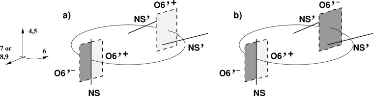
Figure 4: Chiral orientifolds of the IIA brane configuration T-dual to the suspended pinch point singularity. Note that O6^′-planes extend along 7 (but not 89) and NS^′-branes extend along 89 (but not 7).

3.2 Models with one NS-brane and one NS^′-brane

Let us turn to the IIA configurations with one NS-brane and one NS^′-brane. In this case the most obvious possibility is that each fivebrane is mapped to itself, so each is stuck at one orientifold plane. The theories obtained by introducing O6^′-planes and O6-planes are equivalent, and for concreteness we discuss the configuration with O6^′-planes, depicted in figure 5. One of the O6^′-planes is split in halves by the NS-brane, so the configuration contains one fork. There are two field theories, depending on the sign of the O6^′-plane intersected by the NS^′-brane. Choosing for instance the configuration in figure 5b, the resulting field theory is

$$\begin{array}[]{ccc}&SU(n_{1})&\\ A&\raisebox{-3.5pt}{\hbox{\rule{0.4pt}{6.5pt}\hskip-0.4pt\rule{6.5pt}{0.4pt}\hskip-6.5pt\rule[6.5pt]{6.5pt}{0.4pt}}\rule[6.5pt]{0.4pt}{0.4pt}\hskip-0.4pt\rule{0.4pt}{6.5pt}}\hskip-6.9pt\raisebox{3.0pt}{\hbox{\rule{0.4pt}{6.5pt}\hskip-0.4pt\rule{6.5pt}{0.4pt}\hskip-6.5pt\rule[6.5pt]{6.5pt}{0.4pt}}\rule[6.5pt]{0.4pt}{0.4pt}\hskip-0.4pt\rule{0.4pt}{6.5pt}}&\\ {\tilde{A}}&\overline{\raisebox{-3.5pt}{\hbox{\rule{0.4pt}{6.5pt}\hskip-0.4pt\rule{6.5pt}{0.4pt}\hskip-6.5pt\rule[6.5pt]{6.5pt}{0.4pt}}\rule[6.5pt]{0.4pt}{0.4pt}\hskip-0.4pt\rule{0.4pt}{6.5pt}}\hskip-6.9pt\raisebox{3.0pt}{\hbox{\rule{0.4pt}{6.5pt}\hskip-0.4pt\rule{6.5pt}{0.4pt}\hskip-6.5pt\rule[6.5pt]{6.5pt}{0.4pt}}\rule[6.5pt]{0.4pt}{0.4pt}\hskip-0.4pt\rule{0.4pt}{6.5pt}}}&\\ {\tilde{A}}^{\prime}&\overline{\raisebox{-3.5pt}{\hbox{\rule{0.4pt}{6.5pt}\hskip-0.4pt\rule{6.5pt}{0.4pt}\hskip-6.5pt\rule[6.5pt]{6.5pt}{0.4pt}}\rule[6.5pt]{0.4pt}{0.4pt}\hskip-0.4pt\rule{0.4pt}{6.5pt}}\hskip-6.9pt\raisebox{3.0pt}{\hbox{\rule{0.4pt}{6.5pt}\hskip-0.4pt\rule{6.5pt}{0.4pt}\hskip-6.5pt\rule[6.5pt]{6.5pt}{0.4pt}}\rule[6.5pt]{0.4pt}{0.4pt}\hskip-0.4pt\rule{0.4pt}{6.5pt}}}&\\ S^{\prime}&{\raisebox{-0.5pt}{\hbox{\rule{0.4pt}{6.5pt}\hskip-0.4pt\rule{6.5pt}{0.4pt}\hskip-6.5pt\rule[6.5pt]{6.5pt}{0.4pt}}\rule[6.5pt]{0.4pt}{0.4pt}\hskip-0.4pt\rule{0.4pt}{6.5pt}}\hskip-0.4pt\raisebox{-0.5pt}{\hbox{\rule{0.4pt}{6.5pt}\hskip-0.4pt\rule{6.5pt}{0.4pt}\hskip-6.5pt\rule[6.5pt]{6.5pt}{0.4pt}}\rule[6.5pt]{0.4pt}{0.4pt}\hskip-0.4pt\rule{0.4pt}{6.5pt}}}&\\ {\tilde{T}}^{\prime a}&\overline{\raisebox{-0.5pt}{\hbox{\rule{0.4pt}{6.5pt}\hskip-0.4pt\rule{6.5pt}{0.4pt}\hskip-6.5pt\rule[6.5pt]{6.5pt}{0.4pt}}\rule[6.5pt]{0.4pt}{0.4pt}\hskip-0.4pt\rule{0.4pt}{6.5pt}}}&a=1,\ldots,8\\ \end{array}$$ (3.24)

There is a superpotential given by

$$W=A{\tilde{A}}{\tilde{A}}^{\prime}S^{\prime}-S^{\prime}{\tilde{T}}^{\prime}{\tilde{T}}^{\prime}$$ (3.25)

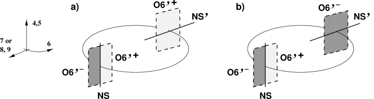
Figure 5: The introduction of O6^′-planes in the IIA brane configuration T-dual to the conifold singularity. The picture appears confusing since we have tried to show too many dimensions in it. The only point to keep in mind is that a NS^′-brane does not split an O6^′-plane in two halves.

A less obvious configuration is possible, in which we consider NS-fivebranes rotated $\pm 45^{0}$ in the 45-89 plane. In such case, an O6^′-plane can map the fivebranes to one another, so they must be located at $\bf Z_{2}$ symmetric positions in $x^{6}$ (note that the configuration with O6-planes provides an equivalent model). We will not consider this case in the present paper.

4 T-dual models I: Orientifolds of $xy=zw^{2}$

Our aim in the rest of the paper is to construct the type IIB T-duals of these configurations. They are expected to be given by suitable orientifolds of the singularities $xy=zw^{2}$ and $xy=zw$. However, it is not obvious how to check this directly. Even though the T-duality allows to guess the action of the orientifold projection on these spaces, the usual techniques to compute the spectrum and to check the cancellation of tadpoles [23, 24, 25, 26, 27, 28] are only valid for models with a solvable worldsheet theory. In this section we show how these difficulties can be overcome, using an indirect approach based on the techniques reviewed in section 2.2.

More concretely, we will construct configurations of D3-branes at orientifolds of $\bf C^{3}/(\bf Z_{2}\times\bf Z_{2})$, and perform partial resolutions of the singular geometry to obtain orientifolds of the SPP and conifold singularities. As in section 2.2, these blow-ups correspond to baryonic branches in the D3-brane field theory. Since the orientifold models are obtained by imposing $\bf Z_{2}$ identifications on the fields in the orbifold theory, any baryonic branch in the orientifold can be regarded as inherited from baryonic branches in the orbifold model. Hence the the map between blow-up modes and baryonic Higgsings we found in section 2.2 will be useful for our analysis. The reverse implication, though, does not work, and certain blow-ups in the orbifold case may be absent, ‘frozen’, in the orientifold models. We will find an example of this in Section 5.

4.1 Some orientifolds of $\bf C^{3}/(\bf Z_{2}\times\bf Z_{2})$

In this section we construct several orientifolds of $\bf C^{3}/(\bf Z_{2}\times\bf Z_{2})$, explicitly checking their consistency (algebraic consistency and cancellation of tadpoles), and computing the field theories arising on D3-brane probes. The list below is not intended to be a complete classification of such models. Rather, it provides us with a rich enough starting point for recovering, upon blowing-up, the field theories obtained in section 3.1 from the IIA perspective. Since the computations of orientifold spectra are rather standard, we leave most of the details out of the discussion, and merely describe the models. Cancellation of tadpoles is discussed in more detail in appendix A. We consider four different models, referred to as A1, A2, B and C.

Models A

We consider the following structure for the orientifold group

$$(1+\theta+\omega+\theta\omega)(1+\Omega^{\prime})$$ (4.1)

where $\Omega^{\prime}=\Omega(-1)^{F_{L}}R_{1}R_{2}R_{3}$. We also take the D3-brane Chan-Paton matrices

$$\gamma_{\theta,3}={\rm diag\,}(i1_{n_{1}},i1_{n_{2}},-i1_{n_{2}},-i1_{n_{1}})$$

$$\gamma_{\omega,3}={\rm diag\,}(i1_{n_{1}},-i1_{n_{2}},i1_{n_{2}},-i1_{n_{1}})$$

$$\gamma_{\Omega^{\prime},3}={\small\left(\begin{array}[]{cccc}&&&1_{n_{1}}\\ &&1_{n_{2}}&\\ &1_{n_{2}}&&\\ 1_{n_{1}}&&&\\ \end{array}\right)}\quad{\rm or}\quad\gamma_{\Omega^{\prime},3}={\small\left(\begin{array}[]{cccc}&&&1_{n_{1}}\\ &&1_{n_{2}}&\\ &-1_{n_{2}}&&\\ -1_{n_{1}}&&&\\ \end{array}\right)}$$ (4.10)

where the choice of $\gamma_{\Omega^{\prime}}$ defines the choice of $SO$ or $Sp$ projection on the D3-branes. We refer to these models as A1 and A2, respectively. The spectra obtained from the orientifold projections are provided below, in eqs. (4.45), (4.51). As discussed in appendix A, this model is consistent without the addition of D7-branes.

Model B

Further models can be obtained by changing the orientifold group. Let us consider

$$(1+\theta+\omega+\theta\omega)(1+\beta\Omega^{\prime})$$ (4.12)

where $\beta:\,(z_{1},z_{2},z_{3})\to(iz_{1},-iz_{2},z_{3})$, that is $\beta^{2}=\theta\omega$. A suitable Chan-Paton embedding is defined by

$$\begin{array}[]{c}\gamma_{\theta,3}={\rm diag\,}(i1_{n_{1}},i1_{n_{2}},-i1_{n_{2}},-i1_{n_{1}})\\ \gamma_{\omega,3}={\rm diag\,}(i1_{n_{1}},-i1_{n_{2}},i1_{n_{2}},-i1_{n_{1}})\end{array} \gamma_{\beta\Omega^{\prime},3}={\small\left(\begin{array}[]{cccc}&&&i\varepsilon_{n_{1}}\\ &&1_{n_{2}}&\\ &-1_{n_{2}}&&\\ -i\varepsilon_{n_{1}}&&&\\ \end{array}\right)}$$ (4.19)

In this case, the matrix $\gamma_{\beta\Omega^{\prime},3}$ is rather unique, and we obtain only one field theory. Its spectrum is given below, in eqs. (4.45), (4.51). As shown in appendix, this models does not require D7-branes for consistency.

Model C

Our last model is constructed using the orientifold group

$$(1+\theta+\omega+\theta\omega)(1+\alpha\Omega^{\prime})$$ (4.20)

where $\alpha:\,(z_{1},z_{2},z_{3})\to(iz_{1},z_{2},-iz_{3})$, that is $\alpha^{2}=\theta$). Our choice of Chan-Paton matrices is

$$\begin{array}[]{c}\gamma_{\theta,3}={\rm diag\,}(i1_{n_{1}},i1_{n_{2}},-i1_{n_{2}},-i1_{n_{1}})\\ \gamma_{\omega,3}={\rm diag\,}(i1_{n_{1}},-i1_{n_{2}},i1_{n_{2}},-i1_{n_{1}})\end{array} \gamma_{\alpha\Omega^{\prime},3}={\small\left(\begin{array}[]{cccc}&&&e^{\frac{\pi i}{4}}1_{n_{1}}\\ &&e^{\frac{\pi i}{4}}1_{n_{2}}&\\ &e^{\frac{3\pi i}{4}}1_{n_{2}}&&\\ e^{\frac{3\pi i}{4}}1_{n_{1}}&&&\\ \end{array}\right)}\quad\quad$$ (4.27)

This model contain non-vanishing Klein bottle tadpoles. As shown in appendix A they can be cancelled by introducing a set of D7₃ branes with Chan-Paton factors:

$$\begin{array}[]{c}\gamma_{\theta,7_{3}}={\rm diag\,}(1_{m_{1}},-1_{m_{2}},-1_{m_{3}},1_{m_{4}})\\ \gamma_{\omega}={\rm diag\,}(1_{m_{1}},-1_{m_{2}},1_{m_{3}},-1_{m-4})\end{array} \gamma_{\alpha\Omega^{\prime}}={\small\left(\begin{array}[]{cccc}\varepsilon_{m_{1}}&&&\\ &1_{m_{2}}&&\\ &&1_{m_{3}}&\\ &&&\varepsilon_{m_{4}}\\ \end{array}\right)}$$ (4.34)

subject to the tadpole cancellation constraint

$$m_{2}-m_{1}=8\quad;\quad m_{3}-m_{4}=8$$ (4.35)

The spectra on the world-volume of the D3-brane probes in all these models are quite similar. Their basic structure is given by

$$\begin{array}[]{ccc}&SU(n_{1})&SU(n_{2})\\ X_{13}&\raisebox{-0.5pt}{\hbox{\rule{0.4pt}{6.5pt}\hskip-0.4pt\rule{6.5pt}{0.4pt}\hskip-6.5pt\rule[6.5pt]{6.5pt}{0.4pt}}\rule[6.5pt]{0.4pt}{0.4pt}\hskip-0.4pt\rule{0.4pt}{6.5pt}}&\raisebox{-0.5pt}{\hbox{\rule{0.4pt}{6.5pt}\hskip-0.4pt\rule{6.5pt}{0.4pt}\hskip-6.5pt\rule[6.5pt]{6.5pt}{0.4pt}}\rule[6.5pt]{0.4pt}{0.4pt}\hskip-0.4pt\rule{0.4pt}{6.5pt}}\\ X_{31}&\overline{\raisebox{-0.5pt}{\hbox{\rule{0.4pt}{6.5pt}\hskip-0.4pt\rule{6.5pt}{0.4pt}\hskip-6.5pt\rule[6.5pt]{6.5pt}{0.4pt}}\rule[6.5pt]{0.4pt}{0.4pt}\hskip-0.4pt\rule{0.4pt}{6.5pt}}}&\overline{\raisebox{-0.5pt}{\hbox{\rule{0.4pt}{6.5pt}\hskip-0.4pt\rule{6.5pt}{0.4pt}\hskip-6.5pt\rule[6.5pt]{6.5pt}{0.4pt}}\rule[6.5pt]{0.4pt}{0.4pt}\hskip-0.4pt\rule{0.4pt}{6.5pt}}}\\ Y_{12}&\raisebox{-0.5pt}{\hbox{\rule{0.4pt}{6.5pt}\hskip-0.4pt\rule{6.5pt}{0.4pt}\hskip-6.5pt\rule[6.5pt]{6.5pt}{0.4pt}}\rule[6.5pt]{0.4pt}{0.4pt}\hskip-0.4pt\rule{0.4pt}{6.5pt}}&\overline{\raisebox{-0.5pt}{\hbox{\rule{0.4pt}{6.5pt}\hskip-0.4pt\rule{6.5pt}{0.4pt}\hskip-6.5pt\rule[6.5pt]{6.5pt}{0.4pt}}\rule[6.5pt]{0.4pt}{0.4pt}\hskip-0.4pt\rule{0.4pt}{6.5pt}}}\\ Y_{21}&\overline{\raisebox{-0.5pt}{\hbox{\rule{0.4pt}{6.5pt}\hskip-0.4pt\rule{6.5pt}{0.4pt}\hskip-6.5pt\rule[6.5pt]{6.5pt}{0.4pt}}\rule[6.5pt]{0.4pt}{0.4pt}\hskip-0.4pt\rule{0.4pt}{6.5pt}}}&\raisebox{-0.5pt}{\hbox{\rule{0.4pt}{6.5pt}\hskip-0.4pt\rule{6.5pt}{0.4pt}\hskip-6.5pt\rule[6.5pt]{6.5pt}{0.4pt}}\rule[6.5pt]{0.4pt}{0.4pt}\hskip-0.4pt\rule{0.4pt}{6.5pt}}\\ Z_{14}&{\rm R}&\\ Z_{41}&{\overline{\rm R}}&\\ Z_{23}&&{\rm R}\\ Z_{32}&&{\overline{\rm R}}\end{array}$$ (4.45)

where ${\rm R}$ represents different two-index tensor representations, which are model-dependent. They are given explicitly in the following table

$$\begin{array}[]{ccccc}&A1&A2&B&C\\ Z_{14}&\raisebox{-3.5pt}{\hbox{\rule{0.4pt}{6.5pt}\hskip-0.4pt\rule{6.5pt}{0.4pt}\hskip-6.5pt\rule[6.5pt]{6.5pt}{0.4pt}}\rule[6.5pt]{0.4pt}{0.4pt}\hskip-0.4pt\rule{0.4pt}{6.5pt}}\hskip-6.9pt\raisebox{3.0pt}{\hbox{\rule{0.4pt}{6.5pt}\hskip-0.4pt\rule{6.5pt}{0.4pt}\hskip-6.5pt\rule[6.5pt]{6.5pt}{0.4pt}}\rule[6.5pt]{0.4pt}{0.4pt}\hskip-0.4pt\rule{0.4pt}{6.5pt}}_{1}&\raisebox{-0.5pt}{\hbox{\rule{0.4pt}{6.5pt}\hskip-0.4pt\rule{6.5pt}{0.4pt}\hskip-6.5pt\rule[6.5pt]{6.5pt}{0.4pt}}\rule[6.5pt]{0.4pt}{0.4pt}\hskip-0.4pt\rule{0.4pt}{6.5pt}}\hskip-0.4pt\raisebox{-0.5pt}{\hbox{\rule{0.4pt}{6.5pt}\hskip-0.4pt\rule{6.5pt}{0.4pt}\hskip-6.5pt\rule[6.5pt]{6.5pt}{0.4pt}}\rule[6.5pt]{0.4pt}{0.4pt}\hskip-0.4pt\rule{0.4pt}{6.5pt}}_{1}&\raisebox{-3.5pt}{\hbox{\rule{0.4pt}{6.5pt}\hskip-0.4pt\rule{6.5pt}{0.4pt}\hskip-6.5pt\rule[6.5pt]{6.5pt}{0.4pt}}\rule[6.5pt]{0.4pt}{0.4pt}\hskip-0.4pt\rule{0.4pt}{6.5pt}}\hskip-6.9pt\raisebox{3.0pt}{\hbox{\rule{0.4pt}{6.5pt}\hskip-0.4pt\rule{6.5pt}{0.4pt}\hskip-6.5pt\rule[6.5pt]{6.5pt}{0.4pt}}\rule[6.5pt]{0.4pt}{0.4pt}\hskip-0.4pt\rule{0.4pt}{6.5pt}}_{1}&\raisebox{-0.5pt}{\hbox{\rule{0.4pt}{6.5pt}\hskip-0.4pt\rule{6.5pt}{0.4pt}\hskip-6.5pt\rule[6.5pt]{6.5pt}{0.4pt}}\rule[6.5pt]{0.4pt}{0.4pt}\hskip-0.4pt\rule{0.4pt}{6.5pt}}\hskip-0.4pt\raisebox{-0.5pt}{\hbox{\rule{0.4pt}{6.5pt}\hskip-0.4pt\rule{6.5pt}{0.4pt}\hskip-6.5pt\rule[6.5pt]{6.5pt}{0.4pt}}\rule[6.5pt]{0.4pt}{0.4pt}\hskip-0.4pt\rule{0.4pt}{6.5pt}}_{1}\\ Z_{41}&\overline{\raisebox{-3.5pt}{\hbox{\rule{0.4pt}{6.5pt}\hskip-0.4pt\rule{6.5pt}{0.4pt}\hskip-6.5pt\rule[6.5pt]{6.5pt}{0.4pt}}\rule[6.5pt]{0.4pt}{0.4pt}\hskip-0.4pt\rule{0.4pt}{6.5pt}}\hskip-6.9pt\raisebox{3.0pt}{\hbox{\rule{0.4pt}{6.5pt}\hskip-0.4pt\rule{6.5pt}{0.4pt}\hskip-6.5pt\rule[6.5pt]{6.5pt}{0.4pt}}\rule[6.5pt]{0.4pt}{0.4pt}\hskip-0.4pt\rule{0.4pt}{6.5pt}}}_{1}&{\overline{\raisebox{-0.5pt}{\hbox{\rule{0.4pt}{6.5pt}\hskip-0.4pt\rule{6.5pt}{0.4pt}\hskip-6.5pt\rule[6.5pt]{6.5pt}{0.4pt}}\rule[6.5pt]{0.4pt}{0.4pt}\hskip-0.4pt\rule{0.4pt}{6.5pt}}\hskip-0.4pt\raisebox{-0.5pt}{\hbox{\rule{0.4pt}{6.5pt}\hskip-0.4pt\rule{6.5pt}{0.4pt}\hskip-6.5pt\rule[6.5pt]{6.5pt}{0.4pt}}\rule[6.5pt]{0.4pt}{0.4pt}\hskip-0.4pt\rule{0.4pt}{6.5pt}}}}_{1}&\overline{\raisebox{-3.5pt}{\hbox{\rule{0.4pt}{6.5pt}\hskip-0.4pt\rule{6.5pt}{0.4pt}\hskip-6.5pt\rule[6.5pt]{6.5pt}{0.4pt}}\rule[6.5pt]{0.4pt}{0.4pt}\hskip-0.4pt\rule{0.4pt}{6.5pt}}\hskip-6.9pt\raisebox{3.0pt}{\hbox{\rule{0.4pt}{6.5pt}\hskip-0.4pt\rule{6.5pt}{0.4pt}\hskip-6.5pt\rule[6.5pt]{6.5pt}{0.4pt}}\rule[6.5pt]{0.4pt}{0.4pt}\hskip-0.4pt\rule{0.4pt}{6.5pt}}}_{1}&\overline{\raisebox{-3.5pt}{\hbox{\rule{0.4pt}{6.5pt}\hskip-0.4pt\rule{6.5pt}{0.4pt}\hskip-6.5pt\rule[6.5pt]{6.5pt}{0.4pt}}\rule[6.5pt]{0.4pt}{0.4pt}\hskip-0.4pt\rule{0.4pt}{6.5pt}}\hskip-6.9pt\raisebox{3.0pt}{\hbox{\rule{0.4pt}{6.5pt}\hskip-0.4pt\rule{6.5pt}{0.4pt}\hskip-6.5pt\rule[6.5pt]{6.5pt}{0.4pt}}\rule[6.5pt]{0.4pt}{0.4pt}\hskip-0.4pt\rule{0.4pt}{6.5pt}}}_{1}\\ Z_{23}&\raisebox{-3.5pt}{\hbox{\rule{0.4pt}{6.5pt}\hskip-0.4pt\rule{6.5pt}{0.4pt}\hskip-6.5pt\rule[6.5pt]{6.5pt}{0.4pt}}\rule[6.5pt]{0.4pt}{0.4pt}\hskip-0.4pt\rule{0.4pt}{6.5pt}}\hskip-6.9pt\raisebox{3.0pt}{\hbox{\rule{0.4pt}{6.5pt}\hskip-0.4pt\rule{6.5pt}{0.4pt}\hskip-6.5pt\rule[6.5pt]{6.5pt}{0.4pt}}\rule[6.5pt]{0.4pt}{0.4pt}\hskip-0.4pt\rule{0.4pt}{6.5pt}}_{2}&\raisebox{-0.5pt}{\hbox{\rule{0.4pt}{6.5pt}\hskip-0.4pt\rule{6.5pt}{0.4pt}\hskip-6.5pt\rule[6.5pt]{6.5pt}{0.4pt}}\rule[6.5pt]{0.4pt}{0.4pt}\hskip-0.4pt\rule{0.4pt}{6.5pt}}\hskip-0.4pt\raisebox{-0.5pt}{\hbox{\rule{0.4pt}{6.5pt}\hskip-0.4pt\rule{6.5pt}{0.4pt}\hskip-6.5pt\rule[6.5pt]{6.5pt}{0.4pt}}\rule[6.5pt]{0.4pt}{0.4pt}\hskip-0.4pt\rule{0.4pt}{6.5pt}}_{2}&\raisebox{-0.5pt}{\hbox{\rule{0.4pt}{6.5pt}\hskip-0.4pt\rule{6.5pt}{0.4pt}\hskip-6.5pt\rule[6.5pt]{6.5pt}{0.4pt}}\rule[6.5pt]{0.4pt}{0.4pt}\hskip-0.4pt\rule{0.4pt}{6.5pt}}\hskip-0.4pt\raisebox{-0.5pt}{\hbox{\rule{0.4pt}{6.5pt}\hskip-0.4pt\rule{6.5pt}{0.4pt}\hskip-6.5pt\rule[6.5pt]{6.5pt}{0.4pt}}\rule[6.5pt]{0.4pt}{0.4pt}\hskip-0.4pt\rule{0.4pt}{6.5pt}}_{2}&\raisebox{-0.5pt}{\hbox{\rule{0.4pt}{6.5pt}\hskip-0.4pt\rule{6.5pt}{0.4pt}\hskip-6.5pt\rule[6.5pt]{6.5pt}{0.4pt}}\rule[6.5pt]{0.4pt}{0.4pt}\hskip-0.4pt\rule{0.4pt}{6.5pt}}\hskip-0.4pt\raisebox{-0.5pt}{\hbox{\rule{0.4pt}{6.5pt}\hskip-0.4pt\rule{6.5pt}{0.4pt}\hskip-6.5pt\rule[6.5pt]{6.5pt}{0.4pt}}\rule[6.5pt]{0.4pt}{0.4pt}\hskip-0.4pt\rule{0.4pt}{6.5pt}}_{2}\\ Z_{32}&\overline{\raisebox{-3.5pt}{\hbox{\rule{0.4pt}{6.5pt}\hskip-0.4pt\rule{6.5pt}{0.4pt}\hskip-6.5pt\rule[6.5pt]{6.5pt}{0.4pt}}\rule[6.5pt]{0.4pt}{0.4pt}\hskip-0.4pt\rule{0.4pt}{6.5pt}}\hskip-6.9pt\raisebox{3.0pt}{\hbox{\rule{0.4pt}{6.5pt}\hskip-0.4pt\rule{6.5pt}{0.4pt}\hskip-6.5pt\rule[6.5pt]{6.5pt}{0.4pt}}\rule[6.5pt]{0.4pt}{0.4pt}\hskip-0.4pt\rule{0.4pt}{6.5pt}}}_{2}&{\overline{\raisebox{-0.5pt}{\hbox{\rule{0.4pt}{6.5pt}\hskip-0.4pt\rule{6.5pt}{0.4pt}\hskip-6.5pt\rule[6.5pt]{6.5pt}{0.4pt}}\rule[6.5pt]{0.4pt}{0.4pt}\hskip-0.4pt\rule{0.4pt}{6.5pt}}\hskip-0.4pt\raisebox{-0.5pt}{\hbox{\rule{0.4pt}{6.5pt}\hskip-0.4pt\rule{6.5pt}{0.4pt}\hskip-6.5pt\rule[6.5pt]{6.5pt}{0.4pt}}\rule[6.5pt]{0.4pt}{0.4pt}\hskip-0.4pt\rule{0.4pt}{6.5pt}}}}_{2}&{\overline{\raisebox{-0.5pt}{\hbox{\rule{0.4pt}{6.5pt}\hskip-0.4pt\rule{6.5pt}{0.4pt}\hskip-6.5pt\rule[6.5pt]{6.5pt}{0.4pt}}\rule[6.5pt]{0.4pt}{0.4pt}\hskip-0.4pt\rule{0.4pt}{6.5pt}}\hskip-0.4pt\raisebox{-0.5pt}{\hbox{\rule{0.4pt}{6.5pt}\hskip-0.4pt\rule{6.5pt}{0.4pt}\hskip-6.5pt\rule[6.5pt]{6.5pt}{0.4pt}}\rule[6.5pt]{0.4pt}{0.4pt}\hskip-0.4pt\rule{0.4pt}{6.5pt}}}}_{2}&\overline{\raisebox{-3.5pt}{\hbox{\rule{0.4pt}{6.5pt}\hskip-0.4pt\rule{6.5pt}{0.4pt}\hskip-6.5pt\rule[6.5pt]{6.5pt}{0.4pt}}\rule[6.5pt]{0.4pt}{0.4pt}\hskip-0.4pt\rule{0.4pt}{6.5pt}}\hskip-6.9pt\raisebox{3.0pt}{\hbox{\rule{0.4pt}{6.5pt}\hskip-0.4pt\rule{6.5pt}{0.4pt}\hskip-6.5pt\rule[6.5pt]{6.5pt}{0.4pt}}\rule[6.5pt]{0.4pt}{0.4pt}\hskip-0.4pt\rule{0.4pt}{6.5pt}}}_{2}\end{array}$$ (4.51)

The model C has additional fields coming from the 3-7₃ sector. For the minimal choice of Chan-Paton matrices satisfying (4.35), $m_{2}=m_{3}=8$, $m_{1}=m_{4}=0$, we have eight fields $T^{a}_{1}$ in the anti-fundamental of $SU(n_{1})$ and eight fields $U^{a}_{2}$ in the anti-fundamental of $SU(n_{2})$. The global $SO(8)^{2}$ global symmetry acting on these flavours is realized on the world-volume of the corresponding D7-branes. The model C is the only chiral one.

Comparing the spectra above with the orbifold spectrum (2.23), we see the effect of the orientifold projection is to identify the groups $SU(n_{1})\leftrightarrow SU(n_{4})$ (in such a way that $\raisebox{-0.5pt}{\hbox{\rule{0.4pt}{6.5pt}\hskip-0.4pt\rule{6.5pt}{0.4pt}\hskip-6.5pt\rule[6.5pt]{6.5pt}{0.4pt}}\rule[6.5pt]{0.4pt}{0.4pt}\hskip-0.4pt\rule{0.4pt}{6.5pt}}_{1}\leftrightarrow\overline{\raisebox{-0.5pt}{\hbox{\rule{0.4pt}{6.5pt}\hskip-0.4pt\rule{6.5pt}{0.4pt}\hskip-6.5pt\rule[6.5pt]{6.5pt}{0.4pt}}\rule[6.5pt]{0.4pt}{0.4pt}\hskip-0.4pt\rule{0.4pt}{6.5pt}}}_{4}$) and $SU(n_{2})\leftrightarrow SU(n_{3})$ (so that $\raisebox{-0.5pt}{\hbox{\rule{0.4pt}{6.5pt}\hskip-0.4pt\rule{6.5pt}{0.4pt}\hskip-6.5pt\rule[6.5pt]{6.5pt}{0.4pt}}\rule[6.5pt]{0.4pt}{0.4pt}\hskip-0.4pt\rule{0.4pt}{6.5pt}}_{2}\leftrightarrow\overline{\raisebox{-0.5pt}{\hbox{\rule{0.4pt}{6.5pt}\hskip-0.4pt\rule{6.5pt}{0.4pt}\hskip-6.5pt\rule[6.5pt]{6.5pt}{0.4pt}}\rule[6.5pt]{0.4pt}{0.4pt}\hskip-0.4pt\rule{0.4pt}{6.5pt}}}_{3}$. This implies the following $\bf Z_{2}$ identification in the fields of the orbifold theory

$$\begin{array}[]{cccc}X_{13}\leftrightarrow X_{24}\;,&Y_{12}\leftrightarrow Y_{34}\;,&Z_{14}\leftrightarrow Z_{14}\;,&Z_{23}\leftrightarrow Z_{23}\;,\\ X_{31}\leftrightarrow X_{42}\;,&Y_{21}\leftrightarrow Y_{43}\;,&Z_{41}\leftrightarrow Z_{41}\;,&Z_{32}\leftrightarrow Z_{32}\;,\end{array}$$ (4.54)

The models A1, A2, B, C differ in the introduction of different signs in this identifications. These are particularly important, since they determine the symmetry of the two-index tensor representations (4.51). However, the relation above contains the relevant information for many purposes. For instance, the basic structure of the superpotential in the orientifold models is obtained from (2.24) upon imposing the identification above.

In the following section we study the different resolutions of these orientifolds. Since the computations are familiar from the orbifold case, we discuss the details only for the most interesting case, the chiral theory, model C. Its superpotential is

$$W={\rm Tr\,}[\;X_{13}^{T}Z_{41}Y_{12}-X_{13}Z_{32}Y_{21}+X_{31}Y_{12}Z_{23}+X_{31}Z_{14}Y_{21}^{T}+Z_{14}UU+Z_{23}TT\;]\quad$$ (4.55)

For future convenience, we also list in the following table the action of the orientifold projection on $\bf C^{3}/(\bf Z_{2}\times\bf Z_{2})$, when described as $xyz=w^{2}$ in terms of the invariant variables $x=z_{1}^{2}$, $y=z_{2}^{2}$, $z=z_{3}^{2}$, $w=z_{1}z_{2}z_{3}$:

$$\begin{array}[]{ccccc}{\rm A1,\;A2}:&x\to x\;,&y\to y\;,&z\to z\;,&w\to-w\\ {\rm B}:&x\to-x\;,&y\to-y\;,&z\to z\;,&w\to-w\\ {\rm C}:&x\to-x\;,&y\to y\;,&z\to-z\;,&w\to-w\\ \end{array}$$ (4.59)

We end this section with a toric comment. Using (2.36), the relations (4.54) show that the orientifold action can be implemented at the level of the $p_{\alpha}$’s of section 2.2.1 as the $\bf Z_{2}$ identification

$$p_{1}\leftrightarrow p_{3}$$ (4.60)

In fact, the relation above does not encode the differences between the models A, B, C. This could be easily accomplished by using matrix-valued fields $p_{\alpha}$, but we will not need this refinement. For future convenience, we note that, given the action of the orientifold on the gauge groups of the orbifold theory (see comment preceding (4.54)), it also imposes the following relation on the FI terms of section 2.2.1

$$\zeta_{1}=-\zeta_{4}\;\;,\;\;\zeta_{2}=-\zeta_{3}$$ (4.61)

where $\zeta_{4}=-\sum_{i=1}^{3}\zeta_{i}$ is the FI for the last $U(1)_{4}$.

4.2 Orientifolds of $xy=zw^{2}$

In this section we perform a single blow-up in the orientifolds of $\bf C^{3}/(\bf Z_{2}\times\bf Z_{2})$ constructed in the previous section, in order to reproduce orientifolds of the suspended pinch point singularity, $xy=zw^{2}$. We show that D3-brane probing the different orientifolds of this singularity realize the different field theories constructed in section 3.1 from the type IIA viewpoint, as orientifolded ${\cal N}=1$ elliptic models. As in [21], these constructions illustrate how several exotic brane dynamics effects on the IIA side have a quite standard realization in the type IIB T-dual setup.

The first observation is that, in order to obtain orientifolds of the SPP variety, the required blow-up must correspond to a vev for one of the fields $Z_{ij}$, rather than to the fields $X_{ij}$ or $Y_{ij}$. This follows from the fact that a vev for one of the latter fields in the orientifold model can be thought to arise from a vev for two fields, related by (4.54), in the orbifold theory. The analysis in section 2.2.1 shows that the associated blow-ups resolve $\bf C^{3}/(\bf Z_{2}\times\bf Z_{2})$ to the $\bf Z_{2}$ orbifold. Orientifolds of $xy=xw^{2}$ are therefore only obtained by following baryonic branches associated to the fields $Z_{ij}$, invariant under (4.54). Let us discuss the models obtained starting with the chiral $\bf C^{3}/(\bf Z_{2}\times\bf Z_{2})$ orientifold, model C.

Consider giving a vev to the symmetric representation $Z_{14}$. From our experience in section 2.2, we know this corresponds to blowing-up by introducing a ${\rm I\kern-1.79993ptP}_{1}$ parametrized by $w^{\prime}=w/z$, so the resulting space is an orientifold of $xy=zw^{\prime 2}$. For readers acquainted with the toric derivation, this is shown exactly as in section 2.2.1: A vev for $Z_{14}$ corresponds to vevs for $p_{6}$, $p_{7}$, $p_{9}$, a possibility which is consistent with the symmetry (4.60). This vevs are forced in the region of FI space given by $\zeta_{1}\gg 0$, $\zeta_{2}=\zeta_{3}=0$, which is consistent with (4.61). The variables invariant under the unbroken symmetries are as in (2.46), $x=p_{1}p_{2}^{2}p_{3}p_{8}$, $y=p_{1}p_{3}p_{4}p_{5}^{2}$, $z=p_{4}p_{8}$, $w^{\prime}=p_{1}p_{2}p_{3}p_{5}=w/z$, satisfying the relation above.

The final model is an orientifold of type IIB string theory on $xy=zw^{\prime 2}$ by $\Omega(-1)^{F_{L}}{\cal R}$, with ${\cal R}$ a geometric $\bf Z_{2}$ transformation inherited from the action (4.59) of the orientifold on $\bf C^{3}/(\bf Z_{2}\times\bf Z_{2})$. We have

$${\cal R}:\quad x\to-x\;\;,\;\;y\to y\;\;,\;\;z\to-z\;\;,\;\;w^{\prime}\to w^{\prime}.$$ (4.62)

This orientifold preserves ${\cal N}=1$ supersymmetry on the D3-branes.

Let us consider the effect of this blow-up in the field theory. The vev for $Z_{14}$ forces the breaking $SU(n_{1})\to SO(n_{1})$. The field $Z_{14}$ is swallowed in the process, and the superpotential (4.55) makes $X_{31}$, $Y_{21}$ and $U^{a}$ massive. The remaining light fields are

$$\begin{array}[]{cccc}&SO(n_{1})&SU(n_{2})&\\ X_{13}&\raisebox{-0.5pt}{\hbox{\rule{0.4pt}{6.5pt}\hskip-0.4pt\rule{6.5pt}{0.4pt}\hskip-6.5pt\rule[6.5pt]{6.5pt}{0.4pt}}\rule[6.5pt]{0.4pt}{0.4pt}\hskip-0.4pt\rule{0.4pt}{6.5pt}}&\raisebox{-0.5pt}{\hbox{\rule{0.4pt}{6.5pt}\hskip-0.4pt\rule{6.5pt}{0.4pt}\hskip-6.5pt\rule[6.5pt]{6.5pt}{0.4pt}}\rule[6.5pt]{0.4pt}{0.4pt}\hskip-0.4pt\rule{0.4pt}{6.5pt}}&\\ Y_{12}&\raisebox{-0.5pt}{\hbox{\rule{0.4pt}{6.5pt}\hskip-0.4pt\rule{6.5pt}{0.4pt}\hskip-6.5pt\rule[6.5pt]{6.5pt}{0.4pt}}\rule[6.5pt]{0.4pt}{0.4pt}\hskip-0.4pt\rule{0.4pt}{6.5pt}}&\overline{\raisebox{-0.5pt}{\hbox{\rule{0.4pt}{6.5pt}\hskip-0.4pt\rule{6.5pt}{0.4pt}\hskip-6.5pt\rule[6.5pt]{6.5pt}{0.4pt}}\rule[6.5pt]{0.4pt}{0.4pt}\hskip-0.4pt\rule{0.4pt}{6.5pt}}}&\\ Z_{41}&\raisebox{-3.5pt}{\hbox{\rule{0.4pt}{6.5pt}\hskip-0.4pt\rule{6.5pt}{0.4pt}\hskip-6.5pt\rule[6.5pt]{6.5pt}{0.4pt}}\rule[6.5pt]{0.4pt}{0.4pt}\hskip-0.4pt\rule{0.4pt}{6.5pt}}\hskip-6.9pt\raisebox{3.0pt}{\hbox{\rule{0.4pt}{6.5pt}\hskip-0.4pt\rule{6.5pt}{0.4pt}\hskip-6.5pt\rule[6.5pt]{6.5pt}{0.4pt}}\rule[6.5pt]{0.4pt}{0.4pt}\hskip-0.4pt\rule{0.4pt}{6.5pt}}&&\\ Z_{23}&&\raisebox{-0.5pt}{\hbox{\rule{0.4pt}{6.5pt}\hskip-0.4pt\rule{6.5pt}{0.4pt}\hskip-6.5pt\rule[6.5pt]{6.5pt}{0.4pt}}\rule[6.5pt]{0.4pt}{0.4pt}\hskip-0.4pt\rule{0.4pt}{6.5pt}}\hskip-0.4pt\raisebox{-0.5pt}{\hbox{\rule{0.4pt}{6.5pt}\hskip-0.4pt\rule{6.5pt}{0.4pt}\hskip-6.5pt\rule[6.5pt]{6.5pt}{0.4pt}}\rule[6.5pt]{0.4pt}{0.4pt}\hskip-0.4pt\rule{0.4pt}{6.5pt}}&\\ Z_{32}&&\overline{\raisebox{-3.5pt}{\hbox{\rule{0.4pt}{6.5pt}\hskip-0.4pt\rule{6.5pt}{0.4pt}\hskip-6.5pt\rule[6.5pt]{6.5pt}{0.4pt}}\rule[6.5pt]{0.4pt}{0.4pt}\hskip-0.4pt\rule{0.4pt}{6.5pt}}\hskip-6.9pt\raisebox{3.0pt}{\hbox{\rule{0.4pt}{6.5pt}\hskip-0.4pt\rule{6.5pt}{0.4pt}\hskip-6.5pt\rule[6.5pt]{6.5pt}{0.4pt}}\rule[6.5pt]{0.4pt}{0.4pt}\hskip-0.4pt\rule{0.4pt}{6.5pt}}}&\\ T_{a}&&\overline{\raisebox{-0.5pt}{\hbox{\rule{0.4pt}{6.5pt}\hskip-0.4pt\rule{6.5pt}{0.4pt}\hskip-6.5pt\rule[6.5pt]{6.5pt}{0.4pt}}\rule[6.5pt]{0.4pt}{0.4pt}\hskip-0.4pt\rule{0.4pt}{6.5pt}}}&a=1,\ldots,8\end{array}$$ (4.70)

Integrating out the massive fields, we obtain the superpotential

$$W={\rm Tr\,}[\,X_{13}^{T}\,Z_{41}\,Y_{12}\,+\,Y_{12}^{T}\,X_{13}\,Z_{32}\,Z_{23}^{T}\,]\,+\,Z_{23}\,T\,T$$ (4.71)

This field theory agrees with that arising from the IIA configuration in figure 4a. Indeed this is supported by some information from the T-duality argument. The T-duality between a IIA models with two NS^′-branes and one NS-brane to the singularity $xy=zw^{\prime 2}$ maps the coordinates 45, 89 to $w^{\prime}$, $z$. Therefore, the orientifold symmetry imposed by the O6^′-planes (reflecting 89, but not 45) T-dualizes to $z\to-z$, $w^{\prime}\to w^{\prime}$, indeed contained in (4.62).

There is another inequivalent Higgsing that can be performed in the model C, given by a vev for one of the antisymmetric representations, say $Z_{41}$. Geometrically, this corresponds again to a blow-up $w^{\prime}=w/z$, leading again to an orientifold of $xy=zw^{\prime 2}$ by $\Omega(-1)^{F_{L}}{\cal R}$, with ${\cal R}$ as above (4.62). The derivation of this result is different, though. In the language of section 2.2.1, the blow up induced by the vev for $Z_{41}$ correspond to vevs for $p_{4}$, $p_{7}$, $p_{8}$ (consistent with (4.60)). This is achieved in the region of FI terms $\zeta_{1}\ll 0$, $\zeta_{2}=\zeta_{3}=0$ (consistent with (4.61)). The invariant variables (2.44) become $x=p_{1}p_{2}^{2}p_{3}p_{9}$, $y=p_{1}p_{3}p_{5}^{2}p_{6}$, $z=p_{6}p_{9}$, and $w=p_{1}p_{2}p_{3}p_{5}p_{6}p_{9}$, and the new invariant is $w^{\prime}=p_{1}p_{2}p_{3}p_{5}=w/z$. They satisfy the relation above.

Given this underlying difference, the field theory on the D3-branes along this baryonic branch differs from (4.70). The group $SU(n_{1})$ breaks to $USp(n_{1})$, $Z_{41}$ is swallowed, and $X_{13}$, $Y_{12}$ get massive. The remaining light fields are

$$\begin{array}[]{cccc}&USp(n_{1})&SU(n_{2})&\\ X_{31}&\raisebox{-0.5pt}{\hbox{\rule{0.4pt}{6.5pt}\hskip-0.4pt\rule{6.5pt}{0.4pt}\hskip-6.5pt\rule[6.5pt]{6.5pt}{0.4pt}}\rule[6.5pt]{0.4pt}{0.4pt}\hskip-0.4pt\rule{0.4pt}{6.5pt}}&\overline{\raisebox{-0.5pt}{\hbox{\rule{0.4pt}{6.5pt}\hskip-0.4pt\rule{6.5pt}{0.4pt}\hskip-6.5pt\rule[6.5pt]{6.5pt}{0.4pt}}\rule[6.5pt]{0.4pt}{0.4pt}\hskip-0.4pt\rule{0.4pt}{6.5pt}}}&\\ Y_{21}&\raisebox{-0.5pt}{\hbox{\rule{0.4pt}{6.5pt}\hskip-0.4pt\rule{6.5pt}{0.4pt}\hskip-6.5pt\rule[6.5pt]{6.5pt}{0.4pt}}\rule[6.5pt]{0.4pt}{0.4pt}\hskip-0.4pt\rule{0.4pt}{6.5pt}}&\raisebox{-0.5pt}{\hbox{\rule{0.4pt}{6.5pt}\hskip-0.4pt\rule{6.5pt}{0.4pt}\hskip-6.5pt\rule[6.5pt]{6.5pt}{0.4pt}}\rule[6.5pt]{0.4pt}{0.4pt}\hskip-0.4pt\rule{0.4pt}{6.5pt}}&\\ Z_{14}&\raisebox{-0.5pt}{\hbox{\rule{0.4pt}{6.5pt}\hskip-0.4pt\rule{6.5pt}{0.4pt}\hskip-6.5pt\rule[6.5pt]{6.5pt}{0.4pt}}\rule[6.5pt]{0.4pt}{0.4pt}\hskip-0.4pt\rule{0.4pt}{6.5pt}}\hskip-0.4pt\raisebox{-0.5pt}{\hbox{\rule{0.4pt}{6.5pt}\hskip-0.4pt\rule{6.5pt}{0.4pt}\hskip-6.5pt\rule[6.5pt]{6.5pt}{0.4pt}}\rule[6.5pt]{0.4pt}{0.4pt}\hskip-0.4pt\rule{0.4pt}{6.5pt}}&&\\ Z_{23}&&\raisebox{-0.5pt}{\hbox{\rule{0.4pt}{6.5pt}\hskip-0.4pt\rule{6.5pt}{0.4pt}\hskip-6.5pt\rule[6.5pt]{6.5pt}{0.4pt}}\rule[6.5pt]{0.4pt}{0.4pt}\hskip-0.4pt\rule{0.4pt}{6.5pt}}\hskip-0.4pt\raisebox{-0.5pt}{\hbox{\rule{0.4pt}{6.5pt}\hskip-0.4pt\rule{6.5pt}{0.4pt}\hskip-6.5pt\rule[6.5pt]{6.5pt}{0.4pt}}\rule[6.5pt]{0.4pt}{0.4pt}\hskip-0.4pt\rule{0.4pt}{6.5pt}}&\\ Z_{32}&&\overline{\raisebox{-3.5pt}{\hbox{\rule{0.4pt}{6.5pt}\hskip-0.4pt\rule{6.5pt}{0.4pt}\hskip-6.5pt\rule[6.5pt]{6.5pt}{0.4pt}}\rule[6.5pt]{0.4pt}{0.4pt}\hskip-0.4pt\rule{0.4pt}{6.5pt}}\hskip-6.9pt\raisebox{3.0pt}{\hbox{\rule{0.4pt}{6.5pt}\hskip-0.4pt\rule{6.5pt}{0.4pt}\hskip-6.5pt\rule[6.5pt]{6.5pt}{0.4pt}}\rule[6.5pt]{0.4pt}{0.4pt}\hskip-0.4pt\rule{0.4pt}{6.5pt}}}&\\ U_{a}&\raisebox{-0.5pt}{\hbox{\rule{0.4pt}{6.5pt}\hskip-0.4pt\rule{6.5pt}{0.4pt}\hskip-6.5pt\rule[6.5pt]{6.5pt}{0.4pt}}\rule[6.5pt]{0.4pt}{0.4pt}\hskip-0.4pt\rule{0.4pt}{6.5pt}}&&a=1,\ldots,8\\ T_{a}&&\overline{\raisebox{-0.5pt}{\hbox{\rule{0.4pt}{6.5pt}\hskip-0.4pt\rule{6.5pt}{0.4pt}\hskip-6.5pt\rule[6.5pt]{6.5pt}{0.4pt}}\rule[6.5pt]{0.4pt}{0.4pt}\hskip-0.4pt\rule{0.4pt}{6.5pt}}}&a=1,\ldots,8\end{array}$$ (4.80)

The superpotential is given by

$$W={\rm Tr\,}[\,X_{31}Z_{14}Y_{21}^{T}\,+\,Y_{21}X_{31}^{T}Z_{23}Z_{32}\,]\,+\,Z_{23}TT\,+\,Z_{14}UU$$ (4.81)

The spectrum suggests the model provides the T-dual of the IIA brane configuration in figure 4b. In fact, the orientifold action on the IIA picture agrees, via T-duality, with the action on the IIB side. However the spectrum (4.80) has additional states as compared with (3.16), concretely eight chiral flavours of $USp(n_{1})$. The precise IIA configuration to which this model T-dualizes must contain eight (whole) D6^′-branes between the NS^′-branes. Notice how the coupling between these flavours and the adjoint of $USp(n_{1})$ in (4.81) is indeed present in the IIA picture.

There are two important lessons to learn from this example. The first is that our method has a small caveat. Even though it yields completely consistent orientifolds of non-orbifold spaces, there is no guarantee that it yields the simplest model for a given orientifold action. In the case above, the IIA picture does not require these D6^′-branes for consistency, and so suggests that the IIB D7-branes responsible for the appearance of the flavours $U$ are not required in the orientifold of the SPP singularity. However, we know they were actually required for consistency of our starting point, the model C. The resolution of the puzzle is that in the process of connecting the orientifold of $\bf C^{3}/(\bf Z_{2}\times\bf Z_{2})$ to the orientifold of the SPP some tadpoles become non-dangerous, the corresponding RR-flux now being able to escape to infinity along the infinitely blown-up ${\rm I\kern-1.79993ptP}_{1}$. In what follows we will always remove this type of additional states whenever they appear.

The second lesson is that in some circumstances one D7-brane in the IIB side can map to one whole D6^′-brane, as in the model above. Notice that the eight D6^′-branes in the IIA picture suffer the projection by the whole O6${}^{\prime}\,{}^{-}$-plane, and so have a $SO(8)$ symmetry, in agreement with the IIB picture.

Since the two models constructed, (4.70) and (4.80), are geometrically the same, but provide different field theories on the probes, we learn that the orientifold $\Omega(-1)^{F_{L}}{\cal R}$, with ${\cal R}$ given by (4.62), allows for two different projections ($SO$ and $Sp$) on the D3-branes.

The analysis we have performed can be applied analogously to the remaining $\bf Z_{2}\times\bf Z_{2}$ orientifolds, models A1, A2 and B. The orientifolds of $xy=zw^{2}$ obtained by the blowing-up procedure reproduce all the field theories proposed in section 3.1, which arise for type IIA configurations with two NS^′-branes and one NS-brane. Moreover, the geometric action of the orientifold projection agrees with the expectations from directly T-dualizing the orientifold action on the IIA models. The results for the different orientifolds are shown in the following table.

$xyz=w^{2}$	Higgsing/Blow-up	$\Omega(-1)^{F_{L}}{\cal R}$ on $xy=zw^{\prime 2}$	Type IIA configuration
A1 $x\to x$, $y\to y$, $z\to z$, $w\to-w$	$\langle Z_{14}\rangle_{\raisebox{-3.5pt}{\hbox{\rule{0.4pt}{3.5pt}\hskip-0.4pt\rule{3.5pt}{0.4pt}\hskip-3.5pt\rule[3.5pt]{3.5pt}{0.4pt}}\rule[3.5pt]{0.4pt}{0.4pt}\hskip-0.4pt\rule{0.4pt}{3.5pt}}\hskip-3.9pt\raisebox{0.0pt}{\hbox{\rule{0.4pt}{3.5pt}\hskip-0.4pt\rule{3.5pt}{0.4pt}\hskip-3.5pt\rule[3.5pt]{3.5pt}{0.4pt}}\rule[3.5pt]{0.4pt}{0.4pt}\hskip-0.4pt\rule{0.4pt}{3.5pt}}}$ $w^{\prime}=w/z$	$x\to x$, $y\to y$, $z\to z$, $w^{\prime}\to-w^{\prime}$	Fig. 3d (O6-, NS)-NS′-O6-
A2 $x\to x$, $y\to y$, $z\to z$, $w\to-w$	$\langle Z_{14}\rangle_{\raisebox{-0.5pt}{\hbox{\rule{0.4pt}{3.5pt}\hskip-0.4pt\rule{3.5pt}{0.4pt}\hskip-3.5pt\rule[3.5pt]{3.5pt}{0.4pt}}\rule[3.5pt]{0.4pt}{0.4pt}\hskip-0.4pt\rule{0.4pt}{3.5pt}}\hskip-0.4pt\raisebox{-0.5pt}{\hbox{\rule{0.4pt}{3.5pt}\hskip-0.4pt\rule{3.5pt}{0.4pt}\hskip-3.5pt\rule[3.5pt]{3.5pt}{0.4pt}}\rule[3.5pt]{0.4pt}{0.4pt}\hskip-0.4pt\rule{0.4pt}{3.5pt}}}$ $w^{\prime}=w/z$	$x\to x$, $y\to y$, $z\to z$, $w^{\prime}\to-w^{\prime}$	Fig. 3a (O6+, NS)-NS′-O6+
B	$\langle Z_{14}\rangle_{\raisebox{-3.5pt}{\hbox{\rule{0.4pt}{3.5pt}\hskip-0.4pt\rule{3.5pt}{0.4pt}\hskip-3.5pt\rule[3.5pt]{3.5pt}{0.4pt}}\rule[3.5pt]{0.4pt}{0.4pt}\hskip-0.4pt\rule{0.4pt}{3.5pt}}\hskip-3.9pt\raisebox{0.0pt}{\hbox{\rule{0.4pt}{3.5pt}\hskip-0.4pt\rule{3.5pt}{0.4pt}\hskip-3.5pt\rule[3.5pt]{3.5pt}{0.4pt}}\rule[3.5pt]{0.4pt}{0.4pt}\hskip-0.4pt\rule{0.4pt}{3.5pt}}}$ $w^{\prime}=w/z$	$x\to-x$, $y\to-y$, $z\to z$, $w^{\prime}\to-w^{\prime}$	Fig. 3b (O6+, NS)-NS′-O6-
$x\to-x$, $y\to-y$, $z\to z$, $w\to-w$	$\langle Z_{23}\rangle_{\raisebox{-0.5pt}{\hbox{\rule{0.4pt}{3.5pt}\hskip-0.4pt\rule{3.5pt}{0.4pt}\hskip-3.5pt\rule[3.5pt]{3.5pt}{0.4pt}}\rule[3.5pt]{0.4pt}{0.4pt}\hskip-0.4pt\rule{0.4pt}{3.5pt}}\hskip-0.4pt\raisebox{-0.5pt}{\hbox{\rule{0.4pt}{3.5pt}\hskip-0.4pt\rule{3.5pt}{0.4pt}\hskip-3.5pt\rule[3.5pt]{3.5pt}{0.4pt}}\rule[3.5pt]{0.4pt}{0.4pt}\hskip-0.4pt\rule{0.4pt}{3.5pt}}}$ $w^{\prime}=w/z$	$x\to-x$, $y\to-y$, $z\to z$, $w^{\prime}\to-w^{\prime}$	Fig. 3c (O6-, NS)-NS′-O6+
C	$\langle Z_{14}\rangle_{\raisebox{-0.5pt}{\hbox{\rule{0.4pt}{3.5pt}\hskip-0.4pt\rule{3.5pt}{0.4pt}\hskip-3.5pt\rule[3.5pt]{3.5pt}{0.4pt}}\rule[3.5pt]{0.4pt}{0.4pt}\hskip-0.4pt\rule{0.4pt}{3.5pt}}\hskip-0.4pt\raisebox{-0.5pt}{\hbox{\rule{0.4pt}{3.5pt}\hskip-0.4pt\rule{3.5pt}{0.4pt}\hskip-3.5pt\rule[3.5pt]{3.5pt}{0.4pt}}\rule[3.5pt]{0.4pt}{0.4pt}\hskip-0.4pt\rule{0.4pt}{3.5pt}}}$ $w^{\prime}=w/z$	$x\to-x$, $y\to y$, $z\to-z$, $w^{\prime}\to w^{\prime}$	Fig. 4a (O6′, NS)-NS′-O6${}^{\prime}\,{}^{+}$
$x\to-x$, $y\to y$, $z\to-z$, $w\to-w$	$\langle Z_{41}\rangle_{\raisebox{-3.5pt}{\hbox{\rule{0.4pt}{3.5pt}\hskip-0.4pt\rule{3.5pt}{0.4pt}\hskip-3.5pt\rule[3.5pt]{3.5pt}{0.4pt}}\rule[3.5pt]{0.4pt}{0.4pt}\hskip-0.4pt\rule{0.4pt}{3.5pt}}\hskip-3.9pt\raisebox{0.0pt}{\hbox{\rule{0.4pt}{3.5pt}\hskip-0.4pt\rule{3.5pt}{0.4pt}\hskip-3.5pt\rule[3.5pt]{3.5pt}{0.4pt}}\rule[3.5pt]{0.4pt}{0.4pt}\hskip-0.4pt\rule{0.4pt}{3.5pt}}}$ $w^{\prime}=w/z$	$x\to-x$, $y\to y$, $z\to-z$, $w^{\prime}\to w^{\prime}$	Fig. 4b (O6′, NS)-NS′-O6${}^{\prime}\,{}^{-}$

In the last column we indicate the objects involved in the corresponding IIA configuration (not including their $\bf Z_{2}$ images), ordered as they appear along the $x^{6}$ interval. Objects enclosed in parentheses are located at the same $x^{6}$ position (for instance, (O6^′-NS corresponds to a fork configuration).

Further blow-ups

In this section we would like to make some comments on further blow-ups. As explained above, baryonic branches associated to fields $X$ or $Y$ arise from two blow-ups in the orbifold theory, which become mapped to each other in the orientifolding process. These can be studied using the toric methods we have described, but their net effect is to introduce a variable $y^{\prime}=y/w^{2}$ (or $x^{\prime}=x/w^{2}$). Hence, this type of blow-up leads to orientifolds of smooth spaces, concretely Taub-NUT spaces. The precise action of the orientifold on the geometry can be computed as in the examples above. These blow-ups have a simple interpretation in terms of the T-dual IIA picture, they correspond to the removal of the two parallel NS^′-branes from the configuration.

The resulting field theories are not uninteresting. After the Higgsing, the IIA configurations in figures 3b, 3c realize the ${\cal N}=4$ $USp(n)$ and $SO(n)$ gauge theories, respectively, as constructed in [44]. In the type IIB picture, the transverse space to the D3-branes, given by the Taub-NUT $xy^{\prime}=z$ times a complex plane parametrized by $w^{\prime}$, is modded out by the orientifold action $\Omega(-1)^{F_{L}}{\cal R}^{\prime}$, with ${\cal R}^{\prime}$ acting as

$$x\to-x\;\;,\;\;y^{\prime}\to-y^{\prime}\;\;,\;\;z\to z\;\;,\;\;w^{\prime}\to-w^{\prime}$$ (4.82)

The model in figure 3a (resp. fig. 3d) realizes an ${\cal N}=2$ $SO(n)$ (resp. $USp(n)$) gauge theories with one symmetric (resp. antisymmetric) hypermultiplet. The $USp(n)$ theory, with four additional hypermultiplet flavours, has appeared in several papers [45, 44]. In the T-dual IIB picture, the geometric action of the orientifold is

$$x\to x\;\;,\;\;y^{\prime}\to y^{\prime}\;\;,\;\;z\to z\;\;,\;\;w^{\prime}\to-w^{\prime}$$ (4.83)

The configurations in figure 4 contain a fork even after the Higgsing. The models are however non-chiral, and actually exhibit an enhanced ${\cal N}=2$ supersymmetry. After the Higgsing, the model in figure 4b (resp. figure 4a) realizes a $USp(n)$ ($SO(n)$) theory with one antisymmetric (symmetric) and four fundamental hypermultiplets. In the type IIB picture the corresponding orientifold action is

$$x\to-x\;\;,\;\;y^{\prime}\to y^{\prime}\;\;,\;\;z\to-z\;\;,\;\;w^{\prime}\to w^{\prime}$$ (4.84)

The ${\cal N}=2$ models above illustrate examples of field theories which can be realized in two different IIA brane constructions. Our analysis shows that their type IIB version also correspond to different orientifold projections .

A different pattern is obtained if we explore blow-ups of the orientifolds of $xy=zw^{\prime\,2}$ associated with vevs for the fields $Z_{ij}$. From the type IIB perspective, we can use the techniques of section 2.2.1 to show that the resulting models are always orientifolds of the $\bf Z_{2}$ orbifold. This can be also understood in the IIA setup, since these blow-ups are realized as the removal along $x^{7}$ of the only NS-brane in the configuration, leaving the two parallel NS^′-branes untouched.

Thus, our techniques allow to recover (in a somewhat complicated fashion) some orientifolds of the $\bf C^{2}/\bf Z_{2}$ orbifold, which can actually be directly constructed, as in [46] for ${\cal N}=2$ orientifolds, or as in [21] for ${\cal N}=1$ orientifolds. This provides a non-trivial consistency check for our procedure, by comparing the orientifold actions derived from the blowing-up technique with the orientifold actions used in the direct construction of the model. We find agreement in all the models considered.

Let us briefly discuss this point in the orientifold of $xy=zw^{\prime 2}$ by $\Omega(-1)^{F_{L}}{\cal R}$, with ${\cal R}$ given in (4.62), with the projection leading to the spectrum (4.70). In this case there are two interesting blow-ups which can be performed. Let us first consider the baryonic branch corresponding to a vev for $Z_{23}$. It can be seen to correspond to the blow-up $x^{\prime}=x/z$, so the resulting space is an orientifold of $x^{\prime}y=w^{\prime\,2}$ by $\Omega(-1)^{F_{L}}$ times the action

$$x^{\prime}\to x^{\prime}\;\;,\;\;y\to y\;\;,\;\;w^{\prime}\to w^{\prime}\;\;,\;\;z\to-z$$ (4.85)

From the field theory point of view, the vev for $Z_{23}$ yields a final (non asymptotically free) ${\cal N}=2$ theory with gauge group $SO(n_{1})\times SO(n_{2})$ with one bifundamental hypermultiplet. This field theory can be directly constructed (in analogy with models in [46]) on the world-volume of D3-branes at an orientifold obtained by modding out $\bf C^{3}$by ${\bf Z_{2}}+\Omega_{3}{\bf Z_{2}}$. Here $\Omega_{3}=\Omega(-1)^{F_{L}}R_{3}$ and recall that $R_{3}$ flips the sign of $z_{3}$, and that the generator $\theta$ of $\bf Z_{2}$ flips the sign of $z_{1}$, $z_{2}$. The action of the orientifolding element $\Omega_{3}$ on the invariant variables $x=z_{1}^{2}$, $y=z_{2}^{2}$, $w=z_{1},z_{2}$, $z=z_{3}$ (satisfying $xy=w^{2}$) is exactly (4.85), in agreement with the result from the blowing-up procedure.

A different blow-up would have been achieved if we had given a vev to $Z_{32}$. This choice can be seen to correspond to the blow-up $y^{\prime}=y/z$, so the final orientifold mods $xy^{\prime}=w^{\prime 2}$ by $\Omega(-1)^{F_{L}}$ times the action

$$x\to-x\;\;,\;\;y\to-y\;\;,\;\;w^{\prime}\to w^{\prime}\;\;,\;\;z\to-z$$ (4.86)

From the field theory point of view, the vev for $Z_{32}$ give a final ${\cal N}=2$ theory with group $SO(n_{1})\times USp(n_{2})$ and one bifundamental and four fundamental $\raisebox{-0.5pt}{\hbox{\rule{0.4pt}{6.5pt}\hskip-0.4pt\rule{6.5pt}{0.4pt}\hskip-6.5pt\rule[6.5pt]{6.5pt}{0.4pt}}\rule[6.5pt]{0.4pt}{0.4pt}\hskip-0.4pt\rule{0.4pt}{6.5pt}}_{2}$ hypermultiplets. This theory can be directly constructed (as in [46]), by modding out D3-branes in flat space by the orientifold group ${\bf Z_{2}}+\Omega_{3}\alpha{\bf Z_{2}}$, with $\alpha:(z_{1},z_{2})\to(iz_{1},-iz_{2})$. The action of the orientifold element $\Omega_{3}\alpha\bf Z_{2}$ on the invariant variables is exactly (4.86). These two examples illustrate how the indirect construction of orientifolds using the blowing-up procedure agrees with the direct construction, when the latter is available.

These two blow-ups are interesting for a different reason. In the T-dual brane picture (figure 4a, they correspond to two different deformations of the fork, corresponding to moving the NS-brane towards positive $x^{7}$ (leaving two positively charged O6^′-planes in the configuration) or towards negative $x^{7}$ (leaving two oppositely charged O6^′-planes). In the type IIB picture these two blow-ups differ by a flop transition, as we show below. This was in fact expected, since the distance in $x^{7}$ between the NS- and NS^′-branes in the IIA configuration is mapped to the Kähler size of the ${\rm I\kern-1.79993ptP}_{1}$ in the IIB picture.

We can use the techniques in section 2.2.1 to show that the two blow-ups above differ by a flop transition. The first one corresponds to the region in FI space $\zeta_{1}\gg 0$, $\zeta_{3}+\zeta_{2}=0$, $\zeta_{2}\gg 0$. Notice this choice of FI is consistent with (4.61), so the blow-up indeed exists in the orientifold model. The D-term equations for the charge matrix ${\tilde{Q}}$ (2.40) are solved by $|p_{4}|^{2}=\zeta_{2}$, $|p_{6}|^{2}=\zeta_{1}$, $|p_{7}|^{2}=|p_{9}|^{2}=\zeta_{1}+\zeta_{2}$ (note that these vevs are invariant under (4.60)). Using (2.36), we see these vevs imply the blow-up is associated with a vev for $Z_{14}$, $Z_{23}$ in the field theory. The second blow-up discussed above corresponds to the region $\zeta_{1}\gg 0$, $\zeta_{3}+\zeta_{2}=0$, $\zeta_{2}\ll 0$. The D-term equations for the $p_{\alpha}$ are satisfied by the vevs $|p_{6}|^{2}=|p_{7}|^{2}=\zeta_{1}-\zeta_{2}$, $|p_{8}|^{2}=-\zeta_{2}$, $|p_{9}|^{2}=\zeta_{1}$, which imply the blow-up corresponds to vev for $Z_{14}$, $Z_{32}$ in the field theory. As claimed above, the only difference between both resolutions is the change of sign for $\zeta_{2}$, which signals a flop transition, as studied in [40, 47].

5 T-dual models II: Orientifolds of the conifold

In principle one could try to obtain orientifolds of the conifold by performing blow-ups in the orientifolds of $\bf C^{3}/(\bf Z_{2}\times\bf Z_{2})$ constructed in section 4.1. However, after exhaustive exploration whose details we spare here it is possible to show that this is not possible. This is due to the constraints (4.61) on the blow-up parameters $\zeta_{i}$, which forbid precisely this type of resolution. This has a simple explanation using the relation between the geometric blow-up and the baryonic Higgsing in the field theory. Recall that, before orientifolding, the blow-up of $\bf C^{3}/(\bf Z_{2}\times\bf Z_{2})$ to the conifold corresponds to a vev to exactly two fields arising from different complex planes (for instance, $Z_{14}$, $Y_{34}$, as in section 2.2). Clearly this type of vev is not invariant under the orientifold symmetry (4.54), which does not relate fields from different complex planes. Therefore, the associated geometric blow-up mode is ‘frozen’ in the orientifold model. A particular consequence of this general argument is the fact, encountered in the previous section, that the orientifolds of the SPP singularity cannot be resolved to orientifolds of the conifold (instead, further blow-ups yield orientifolds of the $\bf Z_{2}$ orbifold).

This problem is rather particular to using $\bf C^{3}/(\bf Z_{2}\times\bf Z_{2})$ as starting point. In this section we show the orientifolds of the conifold are in fact recovered as partial blow-ups of orientifolds of the $\bf C^{3}/(\bf Z_{2}\times\bf Z_{3})$ orbifold.

5.1 The $\bf C^{3}/(\bf Z_{2}\times\bf Z_{3})$ orbifold and its blow-up to the conifold

Let us first discuss the model before the orientifold projection. The action of the $\bf Z_{2}\times\bf Z_{3}$ on $\bf C^{3}$ that we are considering is actually equivalent to that generated by the order six element $\theta$

$$\theta:(z_{1},z_{2},z_{3})\to(e^{2\pi i\frac{1}{6}}z_{1},e^{2\pi i\frac{1}{3}}z_{2},e^{2\pi i\frac{3}{6}})$$ (5.1)

The orbifold is also knows as $\bf Z_{6}^{\prime}$. Using the invariant variables $x=z_{1}^{6}$, $y=z_{2}^{3}$, $z=z_{3}^{2}$, $w=z_{1}z_{2}z_{3}$, the space can also be described as the hypersurface in $\bf C^{4}$ defined by $xy^{2}z^{3}=w^{6}$.

The gauge group on the world-volume of a set of D3-brane probes in this space is $\prod_{i=1}^{6}SU(n_{i})\times U(1)$. There are also eighteen ${\cal N}=1$ matter multiplets, denoted

$$X_{12},X_{23},X_{34},X_{45},X_{56},X_{61}$$

$$Y_{13},Y_{24},Y_{35},Y_{46},Y_{51},Y_{62}$$

$$Z_{14},Z_{25},Z_{36},Z_{41},Z_{52},Z_{63}$$ (5.2)

The subindices $ij$ indicate the field transforms in the $(\raisebox{-0.5pt}{\hbox{\rule{0.4pt}{6.5pt}\hskip-0.4pt\rule{6.5pt}{0.4pt}\hskip-6.5pt\rule[6.5pt]{6.5pt}{0.4pt}}\rule[6.5pt]{0.4pt}{0.4pt}\hskip-0.4pt\rule{0.4pt}{6.5pt}}_{i},\overline{\raisebox{-0.5pt}{\hbox{\rule{0.4pt}{6.5pt}\hskip-0.4pt\rule{6.5pt}{0.4pt}\hskip-6.5pt\rule[6.5pt]{6.5pt}{0.4pt}}\rule[6.5pt]{0.4pt}{0.4pt}\hskip-0.4pt\rule{0.4pt}{6.5pt}}}_{j})$ representation. The superpotential is given by

$$W= {\rm Tr\,}[X_{12}Y_{24}Z_{41}-X_{12}Z_{25}Y_{51}+X_{23}Y_{35}Z_{52}-X_{23}Z_{36}Y_{62}+X_{34}Y_{46}Z_{63}-X_{34}Z_{41}Y_{13}+$$

$$+X_{45}Y_{51}Z_{14}-X_{45}Z_{52}Y_{24}+X_{56}Y_{62}Z_{25}-X_{56}Z_{63}Y_{35}+X_{61}Y_{13}Z_{36}-X_{61}Z_{14}Y_{46}]$$

The moduli space of this theory can be constructed explicitly following the technique in section 2.2.1. Since it does not introduce new conceptual ingredients, we provide the basic data in the appendix B. Following the same arguments as in the $\bf Z_{2}\times\bf Z_{2}$ case, they can be used to reproduce the geometric results mentioned in our arguments below.

Since the process of blowing up to the conifold is somewhat involved, we proceed in two steps. First consider the geometric resolution associated to a vev for $Z_{63}$, $Z_{41}$ (so we are assuming $n_{6}=n_{3},n_{1}=n_{4}$). From the geometric point of view, it corresponds to resolving the $\bf C^{3}/(\bf Z_{2}\times\bf Z_{3})$ orbifold to the singularity $xy=zw^{3}$, as shown in appendix B. From the field theory point of view, the gauge group is broken to $SU(n_{1})\times SU(n_{2})\times SU(n_{3})\times SU(n_{5})$, and the fields $Z_{63}$, $Z_{41}$ are swallowed. The superpotential couplings give masses to the fields $X_{12}$, $X_{34}$, $X_{56}$, $Y_{24}$, $Y_{35}$, and a linear combination of $Y_{46}$, $Y_{13}$. The remaining light fields transform as follows

$$\begin{array}[]{ccccc}&SU(n_{1})&SU(n_{2})&SU(n_{3})&SU(n_{5})\\ Y&\raisebox{-0.5pt}{\hbox{\rule{0.4pt}{6.5pt}\hskip-0.4pt\rule{6.5pt}{0.4pt}\hskip-6.5pt\rule[6.5pt]{6.5pt}{0.4pt}}\rule[6.5pt]{0.4pt}{0.4pt}\hskip-0.4pt\rule{0.4pt}{6.5pt}}&&\overline{\raisebox{-0.5pt}{\hbox{\rule{0.4pt}{6.5pt}\hskip-0.4pt\rule{6.5pt}{0.4pt}\hskip-6.5pt\rule[6.5pt]{6.5pt}{0.4pt}}\rule[6.5pt]{0.4pt}{0.4pt}\hskip-0.4pt\rule{0.4pt}{6.5pt}}}&\\ X_{61}&\overline{\raisebox{-0.5pt}{\hbox{\rule{0.4pt}{6.5pt}\hskip-0.4pt\rule{6.5pt}{0.4pt}\hskip-6.5pt\rule[6.5pt]{6.5pt}{0.4pt}}\rule[6.5pt]{0.4pt}{0.4pt}\hskip-0.4pt\rule{0.4pt}{6.5pt}}}&&\raisebox{-0.5pt}{\hbox{\rule{0.4pt}{6.5pt}\hskip-0.4pt\rule{6.5pt}{0.4pt}\hskip-6.5pt\rule[6.5pt]{6.5pt}{0.4pt}}\rule[6.5pt]{0.4pt}{0.4pt}\hskip-0.4pt\rule{0.4pt}{6.5pt}}&\\ Z_{36}&&&{\rm Adj}&\\ X_{23}&&\raisebox{-0.5pt}{\hbox{\rule{0.4pt}{6.5pt}\hskip-0.4pt\rule{6.5pt}{0.4pt}\hskip-6.5pt\rule[6.5pt]{6.5pt}{0.4pt}}\rule[6.5pt]{0.4pt}{0.4pt}\hskip-0.4pt\rule{0.4pt}{6.5pt}}&\overline{\raisebox{-0.5pt}{\hbox{\rule{0.4pt}{6.5pt}\hskip-0.4pt\rule{6.5pt}{0.4pt}\hskip-6.5pt\rule[6.5pt]{6.5pt}{0.4pt}}\rule[6.5pt]{0.4pt}{0.4pt}\hskip-0.4pt\rule{0.4pt}{6.5pt}}}&\\ Y_{62}&&\overline{\raisebox{-0.5pt}{\hbox{\rule{0.4pt}{6.5pt}\hskip-0.4pt\rule{6.5pt}{0.4pt}\hskip-6.5pt\rule[6.5pt]{6.5pt}{0.4pt}}\rule[6.5pt]{0.4pt}{0.4pt}\hskip-0.4pt\rule{0.4pt}{6.5pt}}}&\raisebox{-0.5pt}{\hbox{\rule{0.4pt}{6.5pt}\hskip-0.4pt\rule{6.5pt}{0.4pt}\hskip-6.5pt\rule[6.5pt]{6.5pt}{0.4pt}}\rule[6.5pt]{0.4pt}{0.4pt}\hskip-0.4pt\rule{0.4pt}{6.5pt}}&\\ Z_{25}&&\raisebox{-0.5pt}{\hbox{\rule{0.4pt}{6.5pt}\hskip-0.4pt\rule{6.5pt}{0.4pt}\hskip-6.5pt\rule[6.5pt]{6.5pt}{0.4pt}}\rule[6.5pt]{0.4pt}{0.4pt}\hskip-0.4pt\rule{0.4pt}{6.5pt}}&&\overline{\raisebox{-0.5pt}{\hbox{\rule{0.4pt}{6.5pt}\hskip-0.4pt\rule{6.5pt}{0.4pt}\hskip-6.5pt\rule[6.5pt]{6.5pt}{0.4pt}}\rule[6.5pt]{0.4pt}{0.4pt}\hskip-0.4pt\rule{0.4pt}{6.5pt}}}\\ Z_{52}&&\overline{\raisebox{-0.5pt}{\hbox{\rule{0.4pt}{6.5pt}\hskip-0.4pt\rule{6.5pt}{0.4pt}\hskip-6.5pt\rule[6.5pt]{6.5pt}{0.4pt}}\rule[6.5pt]{0.4pt}{0.4pt}\hskip-0.4pt\rule{0.4pt}{6.5pt}}}&&\raisebox{-0.5pt}{\hbox{\rule{0.4pt}{6.5pt}\hskip-0.4pt\rule{6.5pt}{0.4pt}\hskip-6.5pt\rule[6.5pt]{6.5pt}{0.4pt}}\rule[6.5pt]{0.4pt}{0.4pt}\hskip-0.4pt\rule{0.4pt}{6.5pt}}\\ X_{45}&\raisebox{-0.5pt}{\hbox{\rule{0.4pt}{6.5pt}\hskip-0.4pt\rule{6.5pt}{0.4pt}\hskip-6.5pt\rule[6.5pt]{6.5pt}{0.4pt}}\rule[6.5pt]{0.4pt}{0.4pt}\hskip-0.4pt\rule{0.4pt}{6.5pt}}&&&\overline{\raisebox{-0.5pt}{\hbox{\rule{0.4pt}{6.5pt}\hskip-0.4pt\rule{6.5pt}{0.4pt}\hskip-6.5pt\rule[6.5pt]{6.5pt}{0.4pt}}\rule[6.5pt]{0.4pt}{0.4pt}\hskip-0.4pt\rule{0.4pt}{6.5pt}}}\\ Y_{51}&\overline{\raisebox{-0.5pt}{\hbox{\rule{0.4pt}{6.5pt}\hskip-0.4pt\rule{6.5pt}{0.4pt}\hskip-6.5pt\rule[6.5pt]{6.5pt}{0.4pt}}\rule[6.5pt]{0.4pt}{0.4pt}\hskip-0.4pt\rule{0.4pt}{6.5pt}}}&&&\raisebox{-0.5pt}{\hbox{\rule{0.4pt}{6.5pt}\hskip-0.4pt\rule{6.5pt}{0.4pt}\hskip-6.5pt\rule[6.5pt]{6.5pt}{0.4pt}}\rule[6.5pt]{0.4pt}{0.4pt}\hskip-0.4pt\rule{0.4pt}{6.5pt}}\\ Z_{14}&{\rm Adj.}&&&\\ \end{array}$$ (5.14)

where $Y$ is the linear combination of $Y_{46}$, $Y_{13}$ which remains massless. The superpotential for these modes is

$$W={\rm Tr\,}[Z_{36}X_{61}Y-Z_{36}Y_{62}X_{23}+X_{23}Y_{62}Z_{25}Z_{52}-Z_{52}Z_{25}Y_{51}X_{45}+X_{45}Y_{51}Z_{14}-Z_{14}YX_{61}]$$

The fact that this field theory appears on the world-volume of D3-branes at the singularity $xy=zw^{3}$ is also supported by the T-duality mentioned in Section 1.1 [9]. The configuration is mapped to a type IIA model containing three NS-branes and one NS^′-brane, with D4-branes suspended among them. This configuration, which shown in figure 6a, allows to easily read off the field theory and interactions above. The picture is also helpful since it suggest that the field theory of the conifold is recovered upon giving vevs to e.g. $X_{45}$, $X_{23}$, since this corresponds to removing two NS-branes from the picture, recovering figure 1. The field theory analysis is straightforward, and we obtain a gauge group $SU(n_{1})\times SU(n_{2})$, with the multiplets $Z_{52}$, $Y$ transforming in the $(\raisebox{-0.5pt}{\hbox{\rule{0.4pt}{6.5pt}\hskip-0.4pt\rule{6.5pt}{0.4pt}\hskip-6.5pt\rule[6.5pt]{6.5pt}{0.4pt}}\rule[6.5pt]{0.4pt}{0.4pt}\hskip-0.4pt\rule{0.4pt}{6.5pt}},\overline{\raisebox{-0.5pt}{\hbox{\rule{0.4pt}{6.5pt}\hskip-0.4pt\rule{6.5pt}{0.4pt}\hskip-6.5pt\rule[6.5pt]{6.5pt}{0.4pt}}\rule[6.5pt]{0.4pt}{0.4pt}\hskip-0.4pt\rule{0.4pt}{6.5pt}}})$, and the multiplets $Z_{25}$, $X_{61}$ in the $(\overline{\raisebox{-0.5pt}{\hbox{\rule{0.4pt}{6.5pt}\hskip-0.4pt\rule{6.5pt}{0.4pt}\hskip-6.5pt\rule[6.5pt]{6.5pt}{0.4pt}}\rule[6.5pt]{0.4pt}{0.4pt}\hskip-0.4pt\rule{0.4pt}{6.5pt}}},\raisebox{-0.5pt}{\hbox{\rule{0.4pt}{6.5pt}\hskip-0.4pt\rule{6.5pt}{0.4pt}\hskip-6.5pt\rule[6.5pt]{6.5pt}{0.4pt}}\rule[6.5pt]{0.4pt}{0.4pt}\hskip-0.4pt\rule{0.4pt}{6.5pt}})$. The superpotential is

$$W={\rm Tr\,}[Z_{52}Z_{25}YX_{61}-Z_{52}X_{61}YZ_{25}]$$ (5.15)

This field theory agrees with (2.4) and (2.64). It is also a simple matter to find the geometric counterpart of this Higgs branch, and find that it corresponds to blowing up $xy=zw^{3}$ to the conifold singularity (see appendix B).

Figure 6: Type IIA brane configurations related by T-duality to D3-branes at the $zy=zw^{3}$ singularity (figure a), and orientifolds thereof (figures b and c).

5.2 Orientifolds of the conifold

Let us turn to the study of orientifold models. We will consider as our starting point the orientifold of $\bf C^{3}/(\bf Z_{2}\times\bf Z_{3})$ obtained by imposing the orientation reversing projection $\Omega^{\prime}\equiv\Omega(-1)^{F_{L}}R_{1}R_{2}R_{3}$ (which preserves ${\cal N}=1$ supersymmetry on the D3-branes. We also choose the following Chan-Paton matrices

$$\gamma_{\theta,3}={\rm diag\,}(e^{\pi i\frac{1}{6}}1_{n_{1}},e^{\pi i\frac{3}{6}}1_{n_{2}},e^{\pi i\frac{5}{6}}1_{n_{3}},e^{\pi i\frac{7}{6}}1_{n_{4}},e^{\pi i\frac{9}{6}}1_{n_{5}},e^{\pi i\frac{11}{6}}1_{n_{6}})$$ (5.16)

$${\footnotesize\gamma_{\Omega^{\prime},3}=\pmatrix{&&&&&1_{n_{1}}\cr&&&&1_{n_{2}}&\cr&&&1_{n_{3}}&&\cr&&1_{n_{3}}&&&\cr&1_{n_{2}}&&&&\cr 1_{n_{1}}&&&&&\cr}\quad{\rm or}\quad\gamma_{\Omega^{\prime},3}=\pmatrix{&&&&&1_{n_{1}}\cr&&&&1_{n_{2}}&\cr&&&1_{n_{3}}&&\cr&&-1_{n_{3}}&&&\cr&-1_{n_{2}}&&&&\cr-1_{n_{1}}&&&&&\cr}}$$

where the choice of $\gamma_{\Omega^{\prime},3}$ determines the type of projection on the D3-branes. This type of models has been studied in [48, 49] in the compact case. For the symmetric $\gamma_{\Omega^{\prime},3}$, the resulting spectrum is

$$\begin{array}[]{cccc}&SU(n_{1})&SU(n_{2})&SU(n_{3})\\ X_{61}&\overline{\raisebox{-3.5pt}{\hbox{\rule{0.4pt}{6.5pt}\hskip-0.4pt\rule{6.5pt}{0.4pt}\hskip-6.5pt\rule[6.5pt]{6.5pt}{0.4pt}}\rule[6.5pt]{0.4pt}{0.4pt}\hskip-0.4pt\rule{0.4pt}{6.5pt}}\hskip-6.9pt\raisebox{3.0pt}{\hbox{\rule{0.4pt}{6.5pt}\hskip-0.4pt\rule{6.5pt}{0.4pt}\hskip-6.5pt\rule[6.5pt]{6.5pt}{0.4pt}}\rule[6.5pt]{0.4pt}{0.4pt}\hskip-0.4pt\rule{0.4pt}{6.5pt}}}&&\\ X_{12}&\raisebox{-0.5pt}{\hbox{\rule{0.4pt}{6.5pt}\hskip-0.4pt\rule{6.5pt}{0.4pt}\hskip-6.5pt\rule[6.5pt]{6.5pt}{0.4pt}}\rule[6.5pt]{0.4pt}{0.4pt}\hskip-0.4pt\rule{0.4pt}{6.5pt}}&\overline{\raisebox{-0.5pt}{\hbox{\rule{0.4pt}{6.5pt}\hskip-0.4pt\rule{6.5pt}{0.4pt}\hskip-6.5pt\rule[6.5pt]{6.5pt}{0.4pt}}\rule[6.5pt]{0.4pt}{0.4pt}\hskip-0.4pt\rule{0.4pt}{6.5pt}}}&\\ X_{23}&&\raisebox{-0.5pt}{\hbox{\rule{0.4pt}{6.5pt}\hskip-0.4pt\rule{6.5pt}{0.4pt}\hskip-6.5pt\rule[6.5pt]{6.5pt}{0.4pt}}\rule[6.5pt]{0.4pt}{0.4pt}\hskip-0.4pt\rule{0.4pt}{6.5pt}}&\overline{\raisebox{-0.5pt}{\hbox{\rule{0.4pt}{6.5pt}\hskip-0.4pt\rule{6.5pt}{0.4pt}\hskip-6.5pt\rule[6.5pt]{6.5pt}{0.4pt}}\rule[6.5pt]{0.4pt}{0.4pt}\hskip-0.4pt\rule{0.4pt}{6.5pt}}}\\ X_{34}&&&\raisebox{-3.5pt}{\hbox{\rule{0.4pt}{6.5pt}\hskip-0.4pt\rule{6.5pt}{0.4pt}\hskip-6.5pt\rule[6.5pt]{6.5pt}{0.4pt}}\rule[6.5pt]{0.4pt}{0.4pt}\hskip-0.4pt\rule{0.4pt}{6.5pt}}\hskip-6.9pt\raisebox{3.0pt}{\hbox{\rule{0.4pt}{6.5pt}\hskip-0.4pt\rule{6.5pt}{0.4pt}\hskip-6.5pt\rule[6.5pt]{6.5pt}{0.4pt}}\rule[6.5pt]{0.4pt}{0.4pt}\hskip-0.4pt\rule{0.4pt}{6.5pt}}\\ Y_{51}&\overline{\raisebox{-0.5pt}{\hbox{\rule{0.4pt}{6.5pt}\hskip-0.4pt\rule{6.5pt}{0.4pt}\hskip-6.5pt\rule[6.5pt]{6.5pt}{0.4pt}}\rule[6.5pt]{0.4pt}{0.4pt}\hskip-0.4pt\rule{0.4pt}{6.5pt}}}&\overline{\raisebox{-0.5pt}{\hbox{\rule{0.4pt}{6.5pt}\hskip-0.4pt\rule{6.5pt}{0.4pt}\hskip-6.5pt\rule[6.5pt]{6.5pt}{0.4pt}}\rule[6.5pt]{0.4pt}{0.4pt}\hskip-0.4pt\rule{0.4pt}{6.5pt}}}&\\ Y_{13}&\raisebox{-0.5pt}{\hbox{\rule{0.4pt}{6.5pt}\hskip-0.4pt\rule{6.5pt}{0.4pt}\hskip-6.5pt\rule[6.5pt]{6.5pt}{0.4pt}}\rule[6.5pt]{0.4pt}{0.4pt}\hskip-0.4pt\rule{0.4pt}{6.5pt}}&&\overline{\raisebox{-0.5pt}{\hbox{\rule{0.4pt}{6.5pt}\hskip-0.4pt\rule{6.5pt}{0.4pt}\hskip-6.5pt\rule[6.5pt]{6.5pt}{0.4pt}}\rule[6.5pt]{0.4pt}{0.4pt}\hskip-0.4pt\rule{0.4pt}{6.5pt}}}\\ Y_{24}&&\raisebox{-0.5pt}{\hbox{\rule{0.4pt}{6.5pt}\hskip-0.4pt\rule{6.5pt}{0.4pt}\hskip-6.5pt\rule[6.5pt]{6.5pt}{0.4pt}}\rule[6.5pt]{0.4pt}{0.4pt}\hskip-0.4pt\rule{0.4pt}{6.5pt}}&\raisebox{-0.5pt}{\hbox{\rule{0.4pt}{6.5pt}\hskip-0.4pt\rule{6.5pt}{0.4pt}\hskip-6.5pt\rule[6.5pt]{6.5pt}{0.4pt}}\rule[6.5pt]{0.4pt}{0.4pt}\hskip-0.4pt\rule{0.4pt}{6.5pt}}\\ Z_{52}&&\overline{\raisebox{-3.5pt}{\hbox{\rule{0.4pt}{6.5pt}\hskip-0.4pt\rule{6.5pt}{0.4pt}\hskip-6.5pt\rule[6.5pt]{6.5pt}{0.4pt}}\rule[6.5pt]{0.4pt}{0.4pt}\hskip-0.4pt\rule{0.4pt}{6.5pt}}\hskip-6.9pt\raisebox{3.0pt}{\hbox{\rule{0.4pt}{6.5pt}\hskip-0.4pt\rule{6.5pt}{0.4pt}\hskip-6.5pt\rule[6.5pt]{6.5pt}{0.4pt}}\rule[6.5pt]{0.4pt}{0.4pt}\hskip-0.4pt\rule{0.4pt}{6.5pt}}}&\\ Z_{25}&&\raisebox{-3.5pt}{\hbox{\rule{0.4pt}{6.5pt}\hskip-0.4pt\rule{6.5pt}{0.4pt}\hskip-6.5pt\rule[6.5pt]{6.5pt}{0.4pt}}\rule[6.5pt]{0.4pt}{0.4pt}\hskip-0.4pt\rule{0.4pt}{6.5pt}}\hskip-6.9pt\raisebox{3.0pt}{\hbox{\rule{0.4pt}{6.5pt}\hskip-0.4pt\rule{6.5pt}{0.4pt}\hskip-6.5pt\rule[6.5pt]{6.5pt}{0.4pt}}\rule[6.5pt]{0.4pt}{0.4pt}\hskip-0.4pt\rule{0.4pt}{6.5pt}}&\\ Z_{14}&\raisebox{-0.5pt}{\hbox{\rule{0.4pt}{6.5pt}\hskip-0.4pt\rule{6.5pt}{0.4pt}\hskip-6.5pt\rule[6.5pt]{6.5pt}{0.4pt}}\rule[6.5pt]{0.4pt}{0.4pt}\hskip-0.4pt\rule{0.4pt}{6.5pt}}&&\overline{\raisebox{-0.5pt}{\hbox{\rule{0.4pt}{6.5pt}\hskip-0.4pt\rule{6.5pt}{0.4pt}\hskip-6.5pt\rule[6.5pt]{6.5pt}{0.4pt}}\rule[6.5pt]{0.4pt}{0.4pt}\hskip-0.4pt\rule{0.4pt}{6.5pt}}}\\ Z_{41}&\overline{\raisebox{-0.5pt}{\hbox{\rule{0.4pt}{6.5pt}\hskip-0.4pt\rule{6.5pt}{0.4pt}\hskip-6.5pt\rule[6.5pt]{6.5pt}{0.4pt}}\rule[6.5pt]{0.4pt}{0.4pt}\hskip-0.4pt\rule{0.4pt}{6.5pt}}}&&\overline{\raisebox{-0.5pt}{\hbox{\rule{0.4pt}{6.5pt}\hskip-0.4pt\rule{6.5pt}{0.4pt}\hskip-6.5pt\rule[6.5pt]{6.5pt}{0.4pt}}\rule[6.5pt]{0.4pt}{0.4pt}\hskip-0.4pt\rule{0.4pt}{6.5pt}}}\end{array}$$ (5.29)

with superpotential

$$W={\rm Tr\,}[\,X_{12}Y_{24}Z_{41}-X_{12}Z_{25}Y_{51}-X_{23}Y_{24}^{T}Z_{52}-X_{23}^{T}Y_{51}Z_{14}-X_{61}Y_{13}Z_{14}^{T}-X_{34}Z_{41}Y_{13}\,].$$

For the antisymmetric $\gamma_{\Omega^{\prime},3}$ the spectrum and interactions are analogous, and can be obtained by replacing the antisymmetric representations in (5.29) by symmetric representations. We will not discuss the details of this case, and mainly treat the case listed above. Also, since we are interested in baryonic Higgs branches which exist only for $n_{1}=n_{2}=n_{3}=n$, from now on we assume equal ranks for all gauge factors.

The orientifold above contains non-vanishing tadpoles which must be cancelled. Notice that the inconsistency arising from these tadpoles is manifest since the field theory has non-abelian gauge anomalies. The simplest possibility to cancel the tadpoles (in the case of equal $n_{i}$’s)is to add a set of D7₂-branes with Chan-Paton matrices

$$\gamma_{\theta,7_{2}}={\rm diag\,}(i1_{4},-i1_{4})\quad;\quad\gamma_{\Omega^{\prime},7_{2}}=\pmatrix{&1_{4}\cr-1_{4}&\cr}$$ (5.30)

The symmetry of the matrix $\gamma_{\Omega^{\prime},7_{2}}$ is determined by that of $\gamma_{\Omega^{\prime},3}$. States in the 3-7₂ sector provide chiral antifundamental multiplets $T_{1}^{a}$, $a=1,\ldots,4$ for $SU(n)_{1}$, and chiral fundamentals $T_{3}^{a}$, $a=1,\ldots,4$ for $SU(n)_{3}$. This additional matter precisely cancels the field theory anomalies. These fields couple to the 33 sector through the superpotential

$$W=T_{1}^{a}Y_{13}T_{3}^{a}$$ (5.31)

For completeness, let us mention that for antisymmetric $\gamma_{\Omega^{\prime},3}$, tadpoles (and anomalies) are cancelled by introducing D7₁-branes with Chan-Paton factors

$$\gamma_{\theta,7_{1}}={\rm diag\,}(1_{4},-1_{4})\quad;\quad\gamma_{\Omega^{\prime},7_{1}}=\pmatrix{1_{4}&\cr&1_{4}\cr}$$ (5.32)

This gives rise to four chiral fundamental flavours for $SU(n_{1})$ and four anti-fundamental flavours for $SU(n_{3})$. They couple to the symmetric representations $X_{61}$ and $X_{34}$.

In the following we would like to describe the blow-up to the orientifold of the conifold. In order to interpret geometrically the Higgsing involved, it will be useful to list here the action of the orientifold symmetry on the fields (5.2) of the orbifold theory

$$\begin{array}[]{ccccc}X_{61}\leftrightarrow X_{61}&&Y_{62}\leftrightarrow Y_{51}&&Z_{52}\leftrightarrow Z_{52}\\ X_{12}\leftrightarrow X_{56}&&Y_{13}\leftrightarrow Y_{46}&&Z_{63}\leftrightarrow Z_{41}\\ X_{23}\leftrightarrow X_{45}&&Y_{24}\leftrightarrow Y_{35}&&Z_{14}\leftrightarrow Z_{36}\\ X_{34}\leftrightarrow X_{34}&&&&Z_{25}\leftrightarrow Z_{25}\end{array}$$ (5.37)

The action on the orbifold space, when described as $xy^{2}z^{3}=w^{6}$, is

$$x\to x\;\;,\;\;y\to-y\;\;,\;\;z\to z\;\;,\;\;w\to-w$$ (5.38)

Finally, it is important for the geometric computations to recall the constraints imposed on the blow-up parameters $\zeta_{i}$, which appear as FI terms or vevs for baryonic operators in the field theory

$$\zeta_{1}=-\zeta_{6}\;\;,\;\;\zeta_{2}=-\zeta_{5}\;\;,\;\;\zeta_{3}=-\zeta_{4}.$$ (5.39)

Let us turn to describing the blowing-up process. Consider a vev for the field $Z_{41}$. Its geometric interpretation is straightforward by regarding it as giving identical vevs to the fields $Z_{41}$, $Z_{63}$ in the orbifold theory, a process which we studied above. This shows that this blow-up will resolve the orientifold of $\bf C^{3}/(\bf Z_{2}\times\bf Z_{3})$ to an orientifold of $xy=zw^{3}$. Following the action (5.38) through the blowing-up up process, the final orientifold acts on $xy=zw^{3}$ as

$$x\to x\;\;,\;\;y\to-y\;\;,\;\;z\to z\;\;,\;\;w\to-w$$ (5.40)

From the field theory point of view, the effect of the Higgsing triggered by this resolution is to break the gauge group to $SU(n)_{1}\times SU(n)_{2}$. The fields $X_{12}$, $Y_{24}$, $X_{34}$ and the antisymmetric part of $Y_{13}$ become massive. The remaining light fields are

$$\begin{array}[]{cccc}&SU(n)_{1}&SU(n)_{2}&\\ X_{23}&\raisebox{-0.5pt}{\hbox{\rule{0.4pt}{6.5pt}\hskip-0.4pt\rule{6.5pt}{0.4pt}\hskip-6.5pt\rule[6.5pt]{6.5pt}{0.4pt}}\rule[6.5pt]{0.4pt}{0.4pt}\hskip-0.4pt\rule{0.4pt}{6.5pt}}&\raisebox{-0.5pt}{\hbox{\rule{0.4pt}{6.5pt}\hskip-0.4pt\rule{6.5pt}{0.4pt}\hskip-6.5pt\rule[6.5pt]{6.5pt}{0.4pt}}\rule[6.5pt]{0.4pt}{0.4pt}\hskip-0.4pt\rule{0.4pt}{6.5pt}}&\\ Y_{51}&\overline{\raisebox{-0.5pt}{\hbox{\rule{0.4pt}{6.5pt}\hskip-0.4pt\rule{6.5pt}{0.4pt}\hskip-6.5pt\rule[6.5pt]{6.5pt}{0.4pt}}\rule[6.5pt]{0.4pt}{0.4pt}\hskip-0.4pt\rule{0.4pt}{6.5pt}}}&\overline{\raisebox{-0.5pt}{\hbox{\rule{0.4pt}{6.5pt}\hskip-0.4pt\rule{6.5pt}{0.4pt}\hskip-6.5pt\rule[6.5pt]{6.5pt}{0.4pt}}\rule[6.5pt]{0.4pt}{0.4pt}\hskip-0.4pt\rule{0.4pt}{6.5pt}}}&\\ X_{61}&\overline{\raisebox{-3.5pt}{\hbox{\rule{0.4pt}{6.5pt}\hskip-0.4pt\rule{6.5pt}{0.4pt}\hskip-6.5pt\rule[6.5pt]{6.5pt}{0.4pt}}\rule[6.5pt]{0.4pt}{0.4pt}\hskip-0.4pt\rule{0.4pt}{6.5pt}}\hskip-6.9pt\raisebox{3.0pt}{\hbox{\rule{0.4pt}{6.5pt}\hskip-0.4pt\rule{6.5pt}{0.4pt}\hskip-6.5pt\rule[6.5pt]{6.5pt}{0.4pt}}\rule[6.5pt]{0.4pt}{0.4pt}\hskip-0.4pt\rule{0.4pt}{6.5pt}}}&&\\ Y_{13}&\raisebox{-0.5pt}{\hbox{\rule{0.4pt}{6.5pt}\hskip-0.4pt\rule{6.5pt}{0.4pt}\hskip-6.5pt\rule[6.5pt]{6.5pt}{0.4pt}}\rule[6.5pt]{0.4pt}{0.4pt}\hskip-0.4pt\rule{0.4pt}{6.5pt}}\hskip-0.4pt\raisebox{-0.5pt}{\hbox{\rule{0.4pt}{6.5pt}\hskip-0.4pt\rule{6.5pt}{0.4pt}\hskip-6.5pt\rule[6.5pt]{6.5pt}{0.4pt}}\rule[6.5pt]{0.4pt}{0.4pt}\hskip-0.4pt\rule{0.4pt}{6.5pt}}&&\\ T^{a}&\overline{\raisebox{-0.5pt}{\hbox{\rule{0.4pt}{6.5pt}\hskip-0.4pt\rule{6.5pt}{0.4pt}\hskip-6.5pt\rule[6.5pt]{6.5pt}{0.4pt}}\rule[6.5pt]{0.4pt}{0.4pt}\hskip-0.4pt\rule{0.4pt}{6.5pt}}}&&a=1,\ldots,8\\ Z_{52}&&\overline{\raisebox{-3.5pt}{\hbox{\rule{0.4pt}{6.5pt}\hskip-0.4pt\rule{6.5pt}{0.4pt}\hskip-6.5pt\rule[6.5pt]{6.5pt}{0.4pt}}\rule[6.5pt]{0.4pt}{0.4pt}\hskip-0.4pt\rule{0.4pt}{6.5pt}}\hskip-6.9pt\raisebox{3.0pt}{\hbox{\rule{0.4pt}{6.5pt}\hskip-0.4pt\rule{6.5pt}{0.4pt}\hskip-6.5pt\rule[6.5pt]{6.5pt}{0.4pt}}\rule[6.5pt]{0.4pt}{0.4pt}\hskip-0.4pt\rule{0.4pt}{6.5pt}}}&\\ Z_{25}&&\raisebox{-3.5pt}{\hbox{\rule{0.4pt}{6.5pt}\hskip-0.4pt\rule{6.5pt}{0.4pt}\hskip-6.5pt\rule[6.5pt]{6.5pt}{0.4pt}}\rule[6.5pt]{0.4pt}{0.4pt}\hskip-0.4pt\rule{0.4pt}{6.5pt}}\hskip-6.9pt\raisebox{3.0pt}{\hbox{\rule{0.4pt}{6.5pt}\hskip-0.4pt\rule{6.5pt}{0.4pt}\hskip-6.5pt\rule[6.5pt]{6.5pt}{0.4pt}}\rule[6.5pt]{0.4pt}{0.4pt}\hskip-0.4pt\rule{0.4pt}{6.5pt}}&\\ Z_{14}&{\rm Adj}&\end{array}$$ (5.50)

where the eight chiral flavours $T^{a}$ arise from the former $T_{1}$ and $T_{3}$. The superpotential is

$$W={\rm Tr\,}[\,Y_{51}X_{23}^{T}Z_{52}Z_{25}+X_{23}^{T}Y_{51}Z_{14}+X_{61}Y_{13}Z_{14}+Y_{13}T^{a}T^{a}\,]$$ (5.51)

This field theory is realized by a type IIA configuration shown in figure 6b. It can be obtained by introducing O6^′-planes in figure 6a. Using the antisymmetric version of $\gamma_{\Omega^{\prime},3}$, one can recover the IIA configuration in figure 6c in complete analogy.

Before proceeding any further, we would like to comment on an interesting point, concerning the origin of the eight fundamental flavours in the final field theory. Recall they arise from the eight half D6^′-branes in the IIA side. On the type IIB model corresponding to symmetric $\gamma_{\Omega^{\prime},3}$, however, these flavour arise from just four D7₂ branes. The matrices (5.30) define four D7₂-branes and their mirror images, leading to a $SU(4)$ gauge symmetry (global symmetry of the superpotential (5.31)). This seems not to agree with previous statements identifying one whole IIB D7-brane with one half IIA D6^′-brane [22, 21]. Also, this structure of IIB D7-branes is rather different with the one we had proposed in Section 4 as the T-dual of the fork configuration. However, a careful analysis of the geometry of the blow-up shows there is no contradiction. Concretely, the D7₂-branes in the initial model span the direction $x$ in $xy^{2}z^{3}=w^{6}$. As shown in the appendix B, the blowing-up process implies the introduction of a new variable $x^{\prime}$ related to $x$ by $x=x^{\prime 2}z$, which is a one-to-two map. Consequently each of the original D7-branes wraps twice the coordinate $x^{\prime}$, and we end up with eight D7-branes spanning the direction $x^{\prime}$ of the space $x^{\prime}y=zw^{\prime 3}$. This description is readily seen to agree with similar geometric realizations of the fork configuration in Section 4. This interpretation is also supported by the fact that for the choice of antisymmetric $\gamma_{\Omega^{\prime},3}$, the initial model already contains eight D7₁-branes. However, since they do not span the direction $x$, they do not suffer this ‘doubling’ process, and provide the right number of T-dual half D6^′-branes. A related interesting feature of this blowing-up process is the accidental enhancement of the D7-brane gauge symmetry from $SU(4)$ (or $SO(4)^{2}$ in the case of antisymmetric $\gamma_{\Omega^{\prime},3}$) to $SO(8)$. It would be nice to gain some additional insight into this issue.

The final blow-up to the orientifold of the conifold corresponds to giving a vev to $X_{23}$. Notice that it has a natural interpretation in the IIA picture, as the removal of two ($\bf Z_{2}$ related) NS-branes, to recover figure 5b. In our geometric description, the effect of such vev is equivalent to the effect of an identical vev for the fields $X_{23}$ and $X_{45}$ in the orbifold model (notice they are related by (5.37). Our analysis above implies that this resolves the orientifold of $xy=zw^{3}$ to an orientifold of $xy=zw$. The precise geometric action on this last space is given by

$$x\to x\;\;,\;\;y\to-y\;\;,\;\;z\to z\;\;,\;\;w\to-w$$ (5.52)

From the field theory point of view, the Higgsing implied by the vev above breaks the gauge group to a single $SU(n)$ factor, with the following matter content

$$X_{61}:\;\;\overline{\raisebox{-3.5pt}{\hbox{\rule{0.4pt}{6.5pt}\hskip-0.4pt\rule{6.5pt}{0.4pt}\hskip-6.5pt\rule[6.5pt]{6.5pt}{0.4pt}}\rule[6.5pt]{0.4pt}{0.4pt}\hskip-0.4pt\rule{0.4pt}{6.5pt}}\hskip-6.9pt\raisebox{3.0pt}{\hbox{\rule{0.4pt}{6.5pt}\hskip-0.4pt\rule{6.5pt}{0.4pt}\hskip-6.5pt\rule[6.5pt]{6.5pt}{0.4pt}}\rule[6.5pt]{0.4pt}{0.4pt}\hskip-0.4pt\rule{0.4pt}{6.5pt}}}\quad;\quad Y_{13}:\;\;\raisebox{-0.5pt}{\hbox{\rule{0.4pt}{6.5pt}\hskip-0.4pt\rule{6.5pt}{0.4pt}\hskip-6.5pt\rule[6.5pt]{6.5pt}{0.4pt}}\rule[6.5pt]{0.4pt}{0.4pt}\hskip-0.4pt\rule{0.4pt}{6.5pt}}\hskip-0.4pt\raisebox{-0.5pt}{\hbox{\rule{0.4pt}{6.5pt}\hskip-0.4pt\rule{6.5pt}{0.4pt}\hskip-6.5pt\rule[6.5pt]{6.5pt}{0.4pt}}\rule[6.5pt]{0.4pt}{0.4pt}\hskip-0.4pt\rule{0.4pt}{6.5pt}}\quad;\quad T^{a}:\;\;\overline{\raisebox{-0.5pt}{\hbox{\rule{0.4pt}{6.5pt}\hskip-0.4pt\rule{6.5pt}{0.4pt}\hskip-6.5pt\rule[6.5pt]{6.5pt}{0.4pt}}\rule[6.5pt]{0.4pt}{0.4pt}\hskip-0.4pt\rule{0.4pt}{6.5pt}}}\quad a=1,\ldots,8$$ (5.53)

$$Z_{52}:\;\;\overline{\raisebox{-3.5pt}{\hbox{\rule{0.4pt}{6.5pt}\hskip-0.4pt\rule{6.5pt}{0.4pt}\hskip-6.5pt\rule[6.5pt]{6.5pt}{0.4pt}}\rule[6.5pt]{0.4pt}{0.4pt}\hskip-0.4pt\rule{0.4pt}{6.5pt}}\hskip-6.9pt\raisebox{3.0pt}{\hbox{\rule{0.4pt}{6.5pt}\hskip-0.4pt\rule{6.5pt}{0.4pt}\hskip-6.5pt\rule[6.5pt]{6.5pt}{0.4pt}}\rule[6.5pt]{0.4pt}{0.4pt}\hskip-0.4pt\rule{0.4pt}{6.5pt}}}\quad;\quad Z_{25}:\;\;\raisebox{-3.5pt}{\hbox{\rule{0.4pt}{6.5pt}\hskip-0.4pt\rule{6.5pt}{0.4pt}\hskip-6.5pt\rule[6.5pt]{6.5pt}{0.4pt}}\rule[6.5pt]{0.4pt}{0.4pt}\hskip-0.4pt\rule{0.4pt}{6.5pt}}\hskip-6.9pt\raisebox{3.0pt}{\hbox{\rule{0.4pt}{6.5pt}\hskip-0.4pt\rule{6.5pt}{0.4pt}\hskip-6.5pt\rule[6.5pt]{6.5pt}{0.4pt}}\rule[6.5pt]{0.4pt}{0.4pt}\hskip-0.4pt\rule{0.4pt}{6.5pt}}$$

with superpotential

$$W={\rm Tr\,}[\,-X_{61}Y_{13}Z_{52}Z_{25}\,]+Y_{13}TT$$ (5.54)

This indeed reproduces the field theory (3.24), arising from the IIA brane configuration in figure 5b. The alternative projection on D3-branes reproduces the field theory realized by the configuration in figure 5a. Finally, let us mention that the geometric action (5.52) is also in agreement with expectations from directly T-dualizing the orientifold action on the IIA side.

Alternative blow-ups

Clearly, many other blow-ups of the initial orientifold of $\bf C^{3}/(\bf Z_{2}\times\bf Z_{3})$ are possible, and performing an exhaustive exploration is outside the point of this paper. Suffice it to say that in all cases we have found results consistent with our proposals in previous sections. For instance, the orientifold of $xy=zw^{3}$ constructed above (with spectrum (5.50)) can be blown up an orientifold of the SPP. More concretely, there are two inequivalent ways to perform such a blow-up, differing by a flop transition. The resulting models correspond to introducing a new ${\rm I\kern-1.79993ptP}_{1}$ parametrized by either $y^{\prime}=y/w$ or $x^{\prime}=x/w$. The two resulting models correspond to modding out the space $xy=zw^{2}$ by $\Omega(-1)^{F_{L}}$ times the geometric actions

$$x\to\pm x\;\;,\;\;y\to\pm y\;\;,\;\;z\to z\;\;,\;\;w\to-w$$ (5.55)

These blow-ups correspond to vevs for $X_{61}$ (for upper signs) or $Y_{13}$ (for lower signs). It is straightforward to obtain the field theories after the Higgsing. In fact, notice that this Higgsings correspond to removing the NS-brane stuck at the fork in figure 6b. The resulting brane configurations are, respectively, given in figures 3d and 3c (up to an irrelevant relabeling of primed and unprimed objects), so the spectrum of the final theories can be read off from them. The geometric action (5.55) is in perfect agreement with the T-duality with these IIA configurations, as can be checked using the actions we had proposed in section 4.2.

A different possibility is to blow-up the orientifold of $\bf C^{3}/(\bf Z_{2}\times\bf Z_{3})$ to an ${\cal N}=1$ orientifold of $\bf C^{3}/\bf Z_{3}$. The direct construction of the latter in [21] provides a new non-trivial check of our procedure. Again, we find agreement between the orientifolds arising after the blow-up, the spectra resulting after the corresponding Higgsing, and the T-dual IIA brane configurations.

6 Final comments

Here we would like to make some comments on the more general case of type IIA brane configurations with $k$ NS-branes, $k^{\prime}$ NS^′-branes, D4-branes and O6^′-planes. The possible models can be easily classified in several families, depending on the parity of the numbers $k$, $k^{\prime}$, and the location of the NS fivebranes with respect to the O6^′-planes. Within each family, there are different field theories depending on the ordering of the NS- and NS^′-branes in the direction 6.

The type IIB T-dual configurations correspond to a set of D3-branes sitting at an orientifold of $xy=z^{k}w^{k^{\prime}}$, with orientifold action $\Omega(-1)^{F_{L}}$ times a geometric $\bf Z_{2}$ symmetry. It is a simple matter to propose suitable $\bf Z_{2}$ geometric actions corresponding to the different type IIA models. The results are shown in table 1. The geometric action of the IIB orientifold on $z$, $w$ follows easily by T-dualizing the action of the IIA orientifold on 89, 45 respectively. The action on $x$, $y$ can be determined from other requirements (the action must be a symmetry of the singularity, the holomorphic 3-form must be odd under it), and consistency with known results (the orientifolds of the conifold and suspended pinch point studied in this paper, as well as the limiting cases where the singularity is actually an orbifold of flat space. Thus, when $k=0$ the T-duals proposed in the table agree with those found in [46], while for $k^{\prime}=0$ the T-duals agree with those proposed in [21]).

	IIB orientifold of $xy=z^{k}w^{k^{\prime}}$	IIA brane configuration
$k$ odd	$x\to x$, $y\to-y$ ∗	(O6${}^{\prime\,+}$, NS′)-NS${}^{(\;)}$${}^{\prime}\;\,$-$\ldots$-NS${}^{(\;)}$${}^{\prime}\;\,$-(NS, O6′)
$k^{\prime}$ odd	$z\to-z$, $w\to w$	(O6${}^{\prime\,-}$, NS′)-NS${}^{(\;)}$${}^{\prime}\;\,$-$\ldots$-NS${}^{(\;)}$${}^{\prime}\;\,$-(NS, O6′)
	$x\to x$, $y\to y$ ∗	O6${}^{\prime\,+}$-NS${}^{(\;)}$${}^{\prime}\;\,$-$\ldots$-NS${}^{(\;)}$${}^{\prime}\;\,$-(NS′, O6${}^{\prime\,+}$)
$k$ even	$z\to-z$, $w\to w$	O6${}^{\prime\,-}$-NS${}^{(\;)}$${}^{\prime}\;\,$-$\ldots$-NS${}^{(\;)}$${}^{\prime}\;\,$-(NS′, O6${}^{\prime\,-}$)
$k^{\prime}$ odd	$x\to-x$, $y\to-y$ ∗	O6${}^{\prime\,+}$-NS${}^{(\;)}$${}^{\prime}\;\,$-$\ldots$-NS${}^{(\;)}$${}^{\prime}\;\,$-(NS′, O6${}^{\prime\,-}$)
	$z\to-z$, $w\to w$	O6${}^{\prime\,-}$-NS${}^{(\;)}$${}^{\prime}\;\,$-$\ldots$-NS${}^{(\;)}$${}^{\prime}\;\,$-(NS′, O6${}^{\prime\,+}$)
$k$ odd	$x\to x$, $y\to-y$ ∗	O6${}^{\prime\,+}$-NS${}^{(\;)}$${}^{\prime}\;\,$-$\ldots$-NS${}^{(\;)}$${}^{\prime}\;\,$-(NS, O6′)
$k^{\prime}$ even	$z\to-z$, $w\to w$	O6${}^{\prime\,-}$-NS${}^{(\;)}$${}^{\prime}\;\,$-$\ldots$-NS${}^{(\;)}$${}^{\prime}\;\,$-(NS, O6′)
	$x\to x$, $y\to y$ ∗	O6${}^{\prime\,+}$-NS${}^{(\;)}$${}^{\prime}\;\,$-$\ldots$-NS${}^{(\;)}$${}^{\prime}\;\,$-O6${}^{\prime\,+}$
	$z\to-z$, $w\to w$	O6${}^{\prime\,-}$-NS${}^{(\;)}$${}^{\prime}\;\,$-$\ldots$-NS${}^{(\;)}$${}^{\prime}\;\,$-O6${}^{\prime\,-}$
	$x\to-x$, $y\to-y$	O6${}^{\prime\,+}$-NS${}^{(\;)}$${}^{\prime}\;\,$-$\ldots$-NS${}^{(\;)}$${}^{\prime}\;\,$-O6${}^{\prime\,-}$
	$z\to-z$, $w\to w$
	$x\to x$, $y\to y$ ∗	(O6${}^{\prime\,+}$, NS′)-NS${}^{(\;)}$${}^{\prime}\;\,$-$\ldots$-NS${}^{(\;)}$${}^{\prime}\;\,$-(NS′, O6${}^{\prime\,+}$)
$k$ even	$z\to-z$, $w\to w$	(O6${}^{\prime\,-}$, NS′)-NS${}^{(\;)}$${}^{\prime}\;\,$-$\ldots$-NS${}^{(\;)}$${}^{\prime}\;\,$-(NS′, O6${}^{\prime\,-}$)
$k^{\prime}$ even	$x\to-x$, $y\to-y$	(O6${}^{\prime\,+}$, NS′)-NS${}^{(\;)}$${}^{\prime}\;\,$-$\ldots$-NS${}^{(\;)}$${}^{\prime}\;\,$-(NS′, O6${}^{\prime\,-}$)
	$z\to-z$, $w\to w$
	$x\to x$, $y\to y$	(O6′, NS)-NS${}^{(\;)}$${}^{\prime}\;\,$-$\ldots$-NS${}^{(\;)}$${}^{\prime}\;\,$-(NS, O6′)
	$z\to-z$, $w\to w$	(parallel forks)
	$x\to-x$, $y\to-y$	(O6′, NS)-NS${}^{(\;)}$${}^{\prime}\;\,$-$\ldots$-NS${}^{(\;)}$${}^{\prime}\;\,$-(NS, O6′)
	$z\to-z$, $w\to w$	(antiparallel forks)

Table 1: The first column of the table shows the type IIB orientifolds T-dual to the type IIA brane configurations shown in the second. The objects in the IIA side are listed as ordered in the coordinates $x^{6}$. Objects enclosed in parentheses are located at the same $x^{6}$ position. NS${}^{(\;)}$${}^{\prime}\;\,$denotes a NS- or a NS^′-brane. Notice that we have not allowed for configurations with coincident fivebranes, since their field theory interpretation is unclear.

The geometric actions in table 1, however, do not completely define the IIB orientifold. In fact, we see that different type IIA configurations may correspond to the same geometric action. As we know from our experience, some of the orientifolds allow for two possible projections ($SO$ and $Sp$) on the D3-branes Chan-Paton factors. This is not a priori obvious from the type IIB side unless one has a more explicit definition of the orientifold. Our procedure of blowing up orientifolds of orbifolds to obtain orientifolds of non-orbifold singularities precisely amounts to such a definition, and this allowed us to claim the existence of these two projections in some models of Section 4.2. In the general case, T-duality predicts the existence of such choice in the orientifolds marked with an asterisk in table 1. This choice should distinguish the T-dual IIB orientifolds of the two IIA configurations shown in the second column.

Another subtle point concerning the precise definition of the IIB orientifold is the action on the closed string modes localized at the singularity (the analogs of the twisted modes in the orbifold case). In particular, some non-orbifold singularities seem to have the analog of $\bf Z_{2}$ twisted sectors, in that the orientifold maps these modes to themselves. In the orientifolds of orbifold singularities it is known that there are two possible projections for these sectors [50]. The orientifold of non-orbifold spaces at hand show a similar feature. This choice should distinguish the IIB orientifolds with identical geometric action, but whose claimed T-dual IIA configurations differ by the location of fivebranes with respect to the O6^′ planes.

Let us mention some further evidence supporting the existence of the mentioned choices in the definition of these orientifolds. In order to do that, notice that any IIA configuration in table 1 without NS^′-branes stuck at the O6^′-planes can be deformed by rotating the NS^′-branes in 45-89 in a way consistent with the orientifold projection. Such models can be thus rotated to models with only NS-branes, D4-branes and O6^′ branes, and no NS^′-branes. The T-duals of these models are D3-branes at ${\cal N}=1$ orientifolds of $\bf C^{2}/\bf Z_{k+k^{\prime}}$ orbifolds [21]. In fact, the whole rotation process can be followed in the type IIB T-dual picture: for generic rotation angles, the T-dual is given by an orientifold of $xy=z^{k}\prod_{i=1}^{k^{\prime}/2}(z-\alpha_{i}w)(z+\alpha_{i}w)$, which interpolates between the space $xy=z^{k}w^{k^{\prime}}$ (for $\alpha_{i}=\infty$) and the orbifold $xy=z^{k+k^{\prime}}$ (for $\alpha_{i}=0$). These orientifolds of $\bf C^{2}/\bf Z_{N}$ orbifolds have been constructed in [21], where it was shown that the different choices in the definition of the IIB orientifold action reproduce the different possible IIA configurations. Table 1 suggests that this feature is preserved along the deformation from the orbifold space to $xy=z^{k}w^{k^{\prime}}$.

Analogously, models without NS-branes stuck at O6^′-planes can be rotated to models without NS-branes. The T-duals of these models are the ${\cal N}=2$ orientifolds of $\bf C^{2}/\bf Z_{N}$ constructed in [46]. The only models which cannot be rotated to more familiar configurations are those with stuck NS- and NS^′-branes, i.e. the case of odd $k$, $k^{\prime}$.

There is a last comment we would like to make concerning this process of brane rotation. Given that it allows to relate orientifolds of these non-orbifold spaces to well-known orientifolds of orbifold spaces, it might be possible to use it to provide a precise definition, and a computational tool to analyze the former. This would allow the analysis of large families of such IIB orientifolds with little effort. In fact this is the situation suggested by the T-duality with IIA configurations: many properties of the rotated model are related to properties of the unrotated one. However, from the IIB perspective there are several difficulties in carrying out this proposal. For instance, it is not clear how the effect of the deformation of the orbifold appears in the field theory of the D3-brane probes. The naive proposal is that some adjoint matter becomes massive and should be integrating out, leaving an effective theory corresponding to the field theory of D3-branes in the deformed space. However reasonable this may seem, in most cases this procedure does not give the correct answer . Thus, until a better understanding of the field theory manifestation of such deformations is achieved, the rotation procedure cannot be claimed to be a good tool to analyze the non-orbifold spaces.

We hope the examples we have worked out illustrate the basic features of the T-duality for IIA configurations with NS- and NS^′-branes. We also expect these results to find applications in other contexts, like for instance the construction of orientifolds of compact Calabi-Yau varieties. Clearly many directions remain to be explored.

Acknowledgements

It is our pleasure to thank J. Erlich, A. Hanany, L. E. Ibáñez, B. Janssen,A. Karch, P. Meessen and A. Naqvi for useful conversations. A. M. U. is grateful to G. Aldazabal and D. Badagnani for their insights into orientifold constructions, and also to M. González for kind encouragement and support, and to the Center for Theoretical Physics at M. I. T. for hospitality. The research of J. P. is supported by the US. Department of Energy under Grant No. DE-FG02-90-ER40542. The research of R. R. is supported by the Ministerio de Educación y Cultura (Spain) under a FPU Grant. The research of A. M. U. is supported by the Ramón Areces Foundation (Spain).

Appendix A Appendix: Tadpole calculation of $Z_{2}\times Z_{2}$ orientifold

Consider the orientifold projection

$$(1+\theta+\omega+\theta\omega)(1+\alpha\Omega^{\prime})$$ (A.1)

with the convention of (4.20). This is the orientifold action of Models B and C. In order to obtain the convention of the Model B adopted in the main text, we have to replace $\alpha$ by $\beta$ and interchange $\theta$ with $\theta\omega$ in the following formulae. We can calculate the tadpole starting from the compact $T^{6}/(\bf Z_{2}\times\bf Z_{2})$ orientifold and then taking the non-compact limit. In this limit, we can ignore the untwisted tadpole and the twisted sector tadpole inversely proportional to one of the volume factors of the three tori. Typically we acquire $\frac{1}{4\sin^{2}(2\pi b_{i})}$ factor in the non-compact limit if an orientifold action is non-trivial on the $i^{th}$ torus, $z_{i}\rightarrow e^{2\pi ib_{i}}z_{i}$. This comes from the momentum modes along the $i^{th}$ torus, which become continuous in the infinite volume limit[28]. One subtlety of $\bf Z_{2}\times\bf Z_{2}$ is that this factor can diverge if corresponding orientifold action acts trivially on the $i^{th}$ plane. This means that the twisted tadpole of our interest is proportional to the volume $V_{i}$ of the $i^{th}$ torus, diverging in the non-compact limit. Such tadpoles should vanish in a consistent configuration. In general, one must consider only the twisted tadpoles proportional to $V_{i}$ and tadpoles independent of any $V_{i}$. Hence, in the $\bf Z_{2}\times\bf Z_{2}$ case, we should consider the tadpoles proportional to $V_{1}$, $V_{2}$ and $V_{3}$, and the tadpoles of order 1 with no volume dependence. We turn to each case in the following.

i) Tadpole proportional to $V_{2}$

This comes from the subset of the orientifold action

$$(1+\theta)(1+\alpha\omega\Omega^{\prime})$$ (A.2)

if we ignore the untwisted tadpole from the cylinder amplitude of D7₁, D7₃-branes. However we should keep all the Klein-bottle and Möbius amplitude since all of them have the same volume dependence $V_{2}$. The amplitude is calculated in the usual manner following[28] and the result is

$$KB: 64\pm 64\,\,\,\,\,(\alpha\omega\Omega^{\prime})$$

$$64\pm 64\,\,\,\,\,(\alpha\theta\omega\Omega^{\prime})$$

$$M: \sum_{i=1,3}-16{\rm Tr\,}(\gamma^{-1}_{\alpha\omega\Omega^{\prime},7_{i}}\gamma^{T}_{\alpha\omega\Omega^{\prime},7_{i}})-16{\rm Tr\,}(\gamma^{-1}_{\alpha\omega\theta\Omega^{\prime},7_{i}}\gamma^{T}_{\alpha\omega\theta\Omega^{\prime},7_{i}})$$

$$C: ({\rm Tr\,}\gamma_{\theta,7_{1}}-{\rm Tr\,}\gamma_{\theta,7_{3}})^{2}.$$

On each column of the Klein bottle amplitude, the first 64 comes from the untwisted sector and the second 64 comes from the $\theta$-twisted sector. For Model C, we choose + sign for the twisted sector contribution. In order to have factorization, one must require

$${\rm Tr\,}(\gamma^{-1}_{\alpha\omega\theta\Omega^{\prime},7_{i}}\gamma^{T}_{\alpha\omega\theta\Omega^{\prime},7_{i}})={\rm Tr\,}(\gamma^{-1}_{\alpha\omega\Omega^{\prime},7_{i}}\gamma^{T}_{\alpha\omega\Omega^{\prime},7_{i}})=\pm{\rm Tr\,}\gamma_{\theta,7_{i}}$$ (A.4)

with $+$ sign for D7₁ branes and $-$ sign for D7₃. Thus we have

$$-{\rm Tr\,}\gamma_{\theta,7_{1}}+{\rm Tr\,}\gamma_{\theta,7_{3}}+16=0.$$ (A.5)

For Model B, we choose the $-$ sign for the twisted sector contribution in the Klein bottle amplitude and use

$${\rm Tr\,}(\gamma^{-1}_{\alpha\omega\theta\Omega^{\prime},7_{i}}\gamma^{T}_{\alpha\omega\theta\Omega^{\prime},7_{i}})=-{\rm Tr\,}(\gamma^{-1}_{\alpha\omega\Omega^{\prime},7_{i}}\gamma^{T}_{\alpha\omega\Omega^{\prime},7_{i}})$$ (A.6)

with $i=1,3$ to make Möbius amplitude vanishing. The only remaining piece is the cylinder amplitude, whose cancellation imposes

$$-{\rm Tr\,}\gamma_{\theta,7_{1}}+{\rm Tr\,}\gamma_{\theta,7_{3}}=0.$$ (A.7)

Now we turn to the other tadpoles. The following analysis holds true both for Model B and Model C.

ii) Tadpoles proportional to $V_{1}$

Only cylinder amplitude contributes and we have

$${\rm Tr\,}\gamma_{\omega,7_{2}}-{\rm Tr\,}\gamma_{\omega,7_{3}}=0.$$ (A.8)

iii) Tadpoles proportional to $V_{3}$

Only cylinder amplitude of D7₁, D7₂ contributes. We have

$${\rm Tr\,}\gamma_{\theta\omega,7_{1}}-{\rm Tr\,}\gamma_{\theta\omega,7_{2}}=0.$$ (A.9)

iv) Tadpoles of order 1

Only the Klein bottle and Möbius amplitudes contribute. For Klein bottle, we evaluate the $\omega$ and $\theta\omega$ twisted amplitudes with insertions of $\alpha\Omega^{\prime}$, $\alpha\theta\Omega^{\prime}$, $\alpha\omega\Omega^{\prime}$, $\alpha\theta\omega\Omega^{\prime}$. If the action of a twist acting along with $\Omega$ is denoted $z_{i}\to e^{2\pi ib_{i}}z_{i}$, the amplitude for the $\omega$ twisted sector is proportional to $\sin 2\pi b_{2}\sin 2\pi b_{3}$. Since $\sin 2\pi b_{2}=0$ for all the orientifold action to be considered in $\bf C^{3}/(\bf Z_{2}\times\bf Z_{2})$, Klein-bottle amplitude vanishes for $\omega$ twisted sector. For $\theta\omega$ twisted sector the amplitude is proportional to $\sin 2\pi b_{1}\sin 2\pi b_{2}$, and vanishes for the same reason.

For the Möbius amplitude, we evaluate $\alpha\Omega^{\prime},\alpha\theta\Omega^{\prime}$ for D7₁, D7₃ branes and $\alpha\omega\Omega^{\prime},\alpha\theta\omega\Omega^{\prime}$ for D7₂ branes. If we T-dualize along $z_{1}$, $z_{2}$ plane for D7₃, along $z_{2}$, $z_{3}$ plane for D7₁ and T-dualize along $z_{1}$, $z_{3}$ planes for D7₂, we end up with $\alpha\theta\omega\Omega^{\prime}$, $\alpha\omega\Omega^{\prime}$ for D3-branes. Denoting by $\theta^{\prime}$ the twist $z_{i}\to e^{2\pi iv_{i}}z_{i}$ that accompanies $\Omega$ in these amplitudes, the Möbius amplitude $\theta^{\prime}\Omega$ for $D3$ brane is proportional to

$$\prod sign(2\pi v_{i})\cos\pi v_{i}$$ (A.10)

In order to obtain the answer for D7₁, D7₃, we put back the zero mode (continuos momemtum mode) contribution in the $z_{1}$, $z_{2}$ planes and $z_{2}$, $z_{3}$ planes, respectively. The amplitude is proportional to

$$\frac{-\cos^{2}\frac{\pi}{4}}{\sin^{2}\frac{3\pi}{4}\sin^{2}\frac{\pi}{2}}{\rm Tr\,}(\gamma^{-1}_{\alpha\Omega^{\prime},7_{i}}\gamma^{T}_{\alpha\Omega^{\prime},7_{i}})+\frac{\cos^{2}\frac{\pi}{4}}{\sin^{2}\frac{3\pi}{4}\sin^{2}\frac{\pi}{2}}{\rm Tr\,}(\gamma^{-1}_{\alpha\theta\Omega^{\prime},7_{i}}\gamma^{T}_{\alpha\theta\Omega^{\prime},7_{i}})$$ (A.11)

with $i=1,3$. The amplitude vanishes if

$${\rm Tr\,}(\gamma^{-1}_{\alpha\Omega^{\prime},7_{i}}\gamma^{T}_{\alpha\Omega^{\prime},7_{i}})={\rm Tr\,}(\gamma^{-1}_{\alpha\theta\Omega^{\prime},7_{i}}\gamma^{T}_{\alpha\theta\Omega^{\prime},7_{i}})\,\,\,\,i=1,3.$$ (A.12)

Similarly, we obtain for D7₂ branes

$${\rm Tr\,}(\gamma^{-1}_{\alpha\omega\Omega^{\prime},7_{2}}\gamma^{T}_{\alpha\omega\Omega^{\prime},7_{2}})={\rm Tr\,}(\gamma^{-1}_{\alpha\theta\omega\Omega^{\prime},7_{2}}\gamma^{T}_{\alpha\theta\omega\Omega^{\prime},7_{2}}).$$ (A.13)

The tadpole cancellation conditions for models B and C are collected in expression (A) for convenience of the reader.

For Model A, the only twisted tadpoles generated by the Klein bottle amplitude are inversely proportional to one of the volume factor $V_{i}$ or, proportional to $V_{i}$ but with vanishing coefficient. This comes from the fermionic zero mode factor $\sin 2\pi b_{1}\sin 2\pi b_{2}$ for $\theta\omega$ twisted sector and similar factors for the others. The Möbius amplitude also vanishes, as we presently explain. If we consider D7₃ branes, we should evaluate $\omega\Omega^{\prime}$, $\theta\Omega^{\prime}$, $\Omega^{\prime}$. This is proportional to

$$(\prod sign(\sin 2\pi v_{i}))\sin\pi v_{1}\sin\pi v_{2}\cos\pi v_{3}$$ (A.14)

where $v_{i}$ defines the twist acting along with $\Omega$. Using the twists appearing in the model, these amplitudes all vanish. Similar reason holds for D7₁- and D7₂-branes.

Finally, the cylinder amplitudes give the condition

$${\rm Tr\,}\gamma_{\theta\omega,7_{1}}-{\rm Tr\,}\gamma_{\theta\omega,7_{2}} = 0$$ (A.15)

$${\rm Tr\,}\gamma_{\omega,7_{2}}-{\rm Tr\,}\gamma_{\omega,7_{3}} = 0$$

$${\rm Tr\,}\gamma_{\theta,7_{3}}-{\rm Tr\,}\gamma_{\theta,7_{1}} = 0$$

To summarize, for Model A,B, and C we obtain the following conditions

$${\rm Tr\,}\gamma_{\theta\omega,7_{1}}-{\rm Tr\,}\gamma_{\theta\omega,7_{2}} = 0\,\,\,\,\,\,(ABC)$$ (A.16)

$${\rm Tr\,}\gamma_{\omega,7_{2}}-{\rm Tr\,}\gamma_{\omega,7_{3}} = 0\,\,\,\,\,(ABC)$$

$${\rm Tr\,}\gamma_{\theta,7_{3}}-{\rm Tr\,}\gamma_{\theta,7_{1}} = 0\,\,\,\,\,(AB)$$

$${\rm Tr\,}\gamma_{\theta,7_{3}}-{\rm Tr\,}\gamma_{\theta,7_{1}} = 16\,\,\,\,\,(C)$$

$${\rm Tr\,}(\gamma^{-1}_{\alpha\Omega^{\prime},7_{i}}\gamma^{T}_{\alpha\Omega^{\prime},7_{i}}) = {\rm Tr\,}(\gamma^{-1}_{\alpha\theta\Omega^{\prime},7_{i}}\gamma^{T}_{\alpha\theta\Omega^{\prime},7_{i}})\,\,\,\,\,(BC)$$ (A.17)

$${\rm Tr\,}(\gamma^{-1}_{\alpha\omega\Omega^{\prime},7_{2}}\gamma^{T}_{\alpha\omega\Omega^{\prime},7_{2}}) = {\rm Tr\,}(\gamma^{-1}_{\alpha\theta\omega\Omega^{\prime},7_{2}}\gamma^{T}_{\alpha\theta\omega\Omega^{\prime},7_{2}})\,\,\,\,\,(BC)$$

$${\rm Tr\,}(\gamma^{-1}_{\alpha\omega\theta\Omega^{\prime},7_{i}}\gamma^{T}_{\alpha\omega\theta\Omega^{\prime},7_{i}}) = -{\rm Tr\,}(\gamma^{-1}_{\alpha\omega\Omega^{\prime},7_{i}}\gamma^{T}_{\alpha\omega\Omega^{\prime},7_{i}})\,\,\,\,\,(B)$$

$${\rm Tr\,}(\gamma^{-1}_{\alpha\omega\theta\Omega^{\prime},7_{i}}\gamma^{T}_{\alpha\omega\theta\Omega^{\prime},7_{i}}) = -{\rm Tr\,}(\gamma^{-1}_{\alpha\omega\Omega^{\prime},7_{i}}\gamma^{T}_{\alpha\omega\Omega^{\prime},7_{i}})=\pm{\rm Tr\,}\gamma_{\theta,7_{i}}\,\,\,\,\,(C)$$

where $i=1,3$ and $+$ sign for D7₁ branes and $-$ sign for D7₃ on the last line. For Model A and B, the above conditions can be satisfied without introducing any D7 branes while for Model C we can introduce only D7₃ branes to satisfy the constraints using the Chan-Paton matrices appearing (4.34). Certainly there are various other solutions. However, they are different from this minimal solution by non-chiral matter contents.

Appendix B Appendix: Moduli space of $\bf C^{3}/(\bf Z_{2}\times\bf Z_{3})$

Following the procedure explained in section 2.2.1, the initial fields (5.2) can be parametrized in terms of seventeen fields $p_{\alpha}$, as follows

$$\begin{array}[]{lll}X_{12}=p_{1}p_{3}p_{4}p_{5}p_{8}p_{9}&Y_{13}=p_{4}p_{5}p_{8}p_{11}p_{15}p_{16}&Z_{14}=p_{5}p_{9}p_{14}p_{16}p_{17}\\ X_{23}=p_{3}p_{6}p_{8}p_{10}p_{15}p_{16}&Y_{24}=p_{7}p_{10}p_{11}p_{15}p_{16}p_{17}&Z_{25}=p_{6}p_{13}p_{14}p_{16}p_{17}\\ X_{34}=p_{1}p_{3}p_{7}p_{9}p_{10}p_{17}&Y_{35}=p_{1}p_{4}p_{7}p_{11}p_{13}p_{17}&Z_{36}=p_{9}p_{12}p_{13}p_{14}p_{17}\\ X_{45}=p_{1}p_{3}p_{4}p_{6}p_{8}p_{13}&Y_{46}=p_{4}p_{8}p_{11}p_{12}p_{13}p_{15}&Z_{41}=p_{2}p_{6}p_{12}p_{13}p_{14}\\ X_{56}=p_{3}p_{8}p_{9}p_{10}p_{12}p_{15}&Y_{51}=p_{2}p_{7}p_{10}p_{11}p_{12}p_{15}&Z_{52}=p_{2}p_{5}p_{9}p_{12}p_{14}\\ X_{61}=p_{1}p_{2}p_{3}p_{6}p_{7}p_{10}&Y_{62}=p_{1}p_{2}p_{4}p_{5}p_{7}p_{11}&Z_{63}=p_{2}p_{5}p_{6}p_{14}p_{16}\end{array}$$ (B.7)

The complete matrix of charges is

$${\tilde{Q}}=\pmatrix{1&0&-1&0&0&0&0&0&0&0&-1&0&0&0&1&0&0&|&0\cr 0&1&0&0&0&0&-1&0&0&0&0&0&0&-1&0&0&1&|&0\cr 0&0&1&-1&0&0&0&0&0&-1&1&0&0&0&0&0&0&|&0\cr 0&0&0&1&-1&0&0&0&0&0&0&0&-1&1&0&0&0&|&0\cr 0&0&0&0&1&0&0&0&-1&0&-1&0&0&0&1&-1&1&|&0\cr 0&0&0&0&0&1&0&0&0&-1&0&0&-1&0&1&-1&1&|&0\cr 0&0&0&0&0&0&1&0&0&-1&-1&0&0&0&1&0&0&|&0\cr 0&0&0&0&0&0&0&1&-1&0&0&1&-1&0&-1&0&1&|&0\cr 0&0&0&0&0&0&0&0&0&0&0&1&0&-1&-1&1&0&|&0\cr 0&-1&0&0&1&0&0&0&0&0&0&0&0&0&0&0&0&|&\zeta_{1}\cr-1&-1&0&0&0&1&1&0&0&0&0&0&0&0&0&0&0&|&\zeta_{2}\cr 1&0&-1&0&-1&0&0&0&1&0&0&0&0&0&0&0&0&|&\zeta_{3}\cr 0&1&0&1&-1&0&-1&0&0&0&0&0&0&0&0&0&0&|&\zeta_{4}\cr-1&1&1&0&0&-1&0&0&0&0&0&0&0&0&0&0&0&|&\zeta_{5}\cr}$$

where the first nine rows define $\bf C^{*}$ actions that remove the redundancy in the parametrization (B.7), and the remaining five implement the five independent $U(1)$ symmetries of the initial field theory.

When the blow-up parameters $\zeta_{i}$ vanish, the kernel of the matrix above is given by

$${\tilde{T}}=\pmatrix{1&0&1&1&0&0&1&1&0&1&1&0&0&-1&1&0&0\cr 0&0&1&-1&0&1&-1&0&1&0&-2&0&0&1&-1&0&0\cr 1&1&1&1&1&1&1&1&1&1&1&1&1&1&1&1&1\cr}$$ (B.8)

The columns of this matrix provide the toric data describing the variety. The polygon defined by the vector endpoints is shown in figure 7. As expected, it corresponds to the toric diagram of $\bf C^{3}/(\bf Z_{2}\times\bf Z_{3})$ .

Figure 7: The toric data for the moduli space of the field theory for D3-branes at the $\bf Z_{2}\times\bf Z_{3}$ singularity.

This space can be described as a hypersurface in $\bf C^{4}$. In order to see that, define the invariant variables

$$\begin{array}[]{ll}x=p_{1}^{4}p_{2}p_{3}^{6}p_{4}^{2}p_{5}p_{6}^{3}p_{7}^{2}p_{8}^{4}p_{9}^{3}p_{10}^{4}p_{12}p_{13}p_{15}^{2}p_{16}p_{17}&(=X_{12}X_{23}X_{34}X_{45}X_{56}X_{61})\\ y=p_{1}p_{2}p_{4}^{2}p_{5}p_{7}^{2}p_{8}p_{10}p_{11}^{3}p_{12}p_{13}p_{15}^{2}p_{16}p_{17}&(=Y_{24}Y_{46}Y_{62})\\ z=p_{2}p_{5}p_{6}p_{9}p_{12}p_{13}p_{14}^{2}p_{16}p_{17}&(=Z_{14}Z_{41})\\ w=p_{1}p_{2}p_{3}p_{4}p_{5}p_{6}p_{7}p_{8}p_{9}p_{10}p_{11}p_{12}p_{13}p_{14}p_{15}p_{16}p_{17}&(=X_{12}Y_{24}Z_{41})\end{array}$$ (B.13)

which satisfy

$$xy^{2}z^{3}=w^{6}$$ (B.14)

This space is precisely $\bf C^{3}/(\bf Z_{2}\times\bf Z_{3})$ , as shown in the main text, after equation (5.1).

Some interesting resolutions

Some interesting blow-ups of this singularity are mentioned in the main text, and we provide here some details of the computations involved. Using equation (B.7), we see the blow-up associated to a vev for the fields $Z_{63}$, $Z_{41}$ is obtained when the fields $p_{2}$, $p_{5}$, $p_{6}$, $p_{12}$, $p_{13}$, $p_{14}$, $p_{16}$ are non-zero. This is achieved in the region of FI space defined by$\zeta_{1}=-\zeta_{4}\ll 0$, $\zeta_{2}=\zeta_{5}=0$, $\zeta_{3}\ll 0$, since the D-terms from the matrix (B) require

$$|p_{2}|^{2}=|p_{6}|^{2}=|p_{14}|^{2}=-\zeta_{3}-\zeta_{1},\quad|p_{5}|^{2}=|p_{16}|^{2}=-\zeta_{3},\quad|p_{12}|^{2}=|p_{13}|^{2}=-\zeta_{1}.$$ (B.15)

The basic invariants under the surviving $U(1)$ symmetries are

$$x^{\prime} = p_{1}^{2}p_{3}^{3}p_{4}p_{7}p_{8}^{2}p_{9}p_{10}^{2}p_{15}$$

$$y = p_{1}p_{4}^{2}p_{7}^{2}p_{8}p_{10}p_{11}^{3}p_{15}^{2}p_{17}$$

$$z = p_{9}p_{17}$$

$$w^{\prime} = p_{1}p_{3}p_{4}p_{7}p_{8}p_{10}p_{11}p_{15}$$ (B.16)

Comparing with the original invariants (B.13), the blow-up implies the redefinition $x=x^{\prime\,2}z$, $w=w^{\prime}z$. The remaining singularity is therefore $x^{\prime}y=zw^{\prime 3}$.

An interesting further blow-up is achieved by vevs for the fields $X_{45}$, $X_{23}$. Using (B.7) this implies that we only keep $p_{7}$, $p_{9}$, $p_{11}$, $p_{17}$ as dynamical, while all other variables get non-zero vev. This vevs can be achieved in the region of FI space defined by $\zeta_{5}=-\zeta_{1}-\zeta_{4}$, $-\zeta_{3}\gg\zeta_{2}\gg 0$, $\zeta_{4}\gg-\zeta_{1}\gg 0$. The D-term equations associated to the charge matrix (B) are satisfied for

$$\begin{array}[]{ll}|p_{1}|^{2}=|p_{4}|^{2}=\zeta_{1}+\zeta_{4}&|p_{10}|^{2}=|p_{15}|^{2}=\zeta_{2}\\ |p_{2}|^{2}=|p_{14}|^{2}=-\zeta_{1}-\zeta_{2}-\zeta_{3}&|p_{12}|^{2}=-\zeta_{1}\\ |p_{3}|^{2}=|p_{8}|^{2}=\zeta_{1}+\zeta_{2}+\zeta_{4}&|p_{13}|^{2}=\zeta_{4}\\ |p_{5}|^{2}=-\zeta_{2}-\zeta_{3}&|p_{16}|^{2}=-\zeta_{3}\\ |p_{6}|^{2}=\zeta_{4}-\zeta_{3}&\end{array}$$ (B.22)

The variables (B.16) become

$$x^{\prime}=p_{7}p_{9}\;\;,\;\;y=p_{7}^{2}p_{11}^{3}p_{17}\;\;,\;\;z=p_{9}p_{17}\;\;,\;\;w^{\prime}=p_{7}p_{11}$$ (B.23)

The new invariant is $y^{\prime}=p_{11}p_{17}=y/w^{\prime 2}$. The remaining singularity is the conifold $x^{\prime}y^{\prime}=zw^{\prime}$.

Appendix C Appendix: Tadpoles for the $\bf Z_{2}\times\bf Z_{3}$ orientifold

As mentioned in the main text, the $\bf C^{3}/(\bf Z_{2}\times\bf Z_{3})$ orbifold is actually isomorphic to the $\bf Z_{6}$ orbifold generated by the action on $\bf C^{3}$ given by $z_{i}\to e^{2\pi iv_{i}}z_{i}$ with $v=(1,2,-3)/6$. The non-compact orientifold studied in section 5.2 belongs to a large family of models, introduced in [51], whose tadpoles can be computed in a quite general fashion. So let us consider a general $\bf Z_{N}$ orbifold, with $N$ even, and generator defined by $v=(\ell_{1},\ell_{2},\ell_{3})/N$, with $\ell_{1}$, $\ell_{3}$ odd and $\ell_{1}+\ell_{2}+\ell_{3}=0$. We mod out this space by the orientifold action $\Omega^{\prime}=\Omega(-1)^{F_{L}}R_{1}R_{2}R_{3}$. We also choose the Chan-Paton matrices $\gamma_{\theta,3}$ ($\gamma_{\theta,7_{2}}$) to have $n_{j}$ ($m_{j}$) eigenvalues $e^{\pi i(2j-1)/N}$, and $\gamma_{\theta,7_{1}}$ ($\gamma_{\theta,7_{3}}$) to have $w_{j}$ ($r_{j}$) eigenvalues $e^{2\pi ij/N}$. The orientifold symmetry imposes $n_{j}=n_{-j+1}$, $m_{j}=m_{-j+1}$, $w_{j}=w_{-j}$, $r_{j}=r_{-j}$.

The gauge group on the D3-branes is $\prod_{i=1}^{N/2}SU(n_{i})$. The matter multiplets can be obtained from the orbifold spectrum

$$\sum_{\alpha=1}^{3}\sum_{i=1}^{N}(\raisebox{-0.5pt}{\hbox{\rule{0.4pt}{6.5pt}\hskip-0.4pt\rule{6.5pt}{0.4pt}\hskip-6.5pt\rule[6.5pt]{6.5pt}{0.4pt}}\rule[6.5pt]{0.4pt}{0.4pt}\hskip-0.4pt\rule{0.4pt}{6.5pt}}_{i},\overline{\raisebox{-0.5pt}{\hbox{\rule{0.4pt}{6.5pt}\hskip-0.4pt\rule{6.5pt}{0.4pt}\hskip-6.5pt\rule[6.5pt]{6.5pt}{0.4pt}}\rule[6.5pt]{0.4pt}{0.4pt}\hskip-0.4pt\rule{0.4pt}{6.5pt}}}_{i+\l_{\alpha}})+\sum_{i=1}^{N}\,[\,(\raisebox{-0.5pt}{\hbox{\rule{0.4pt}{6.5pt}\hskip-0.4pt\rule{6.5pt}{0.4pt}\hskip-6.5pt\rule[6.5pt]{6.5pt}{0.4pt}}\rule[6.5pt]{0.4pt}{0.4pt}\hskip-0.4pt\rule{0.4pt}{6.5pt}}_{i},{\overline{m}}_{i+\frac{\ell_{1}+\ell_{3}}{2}})+(\raisebox{-0.5pt}{\hbox{\rule{0.4pt}{6.5pt}\hskip-0.4pt\rule{6.5pt}{0.4pt}\hskip-6.5pt\rule[6.5pt]{6.5pt}{0.4pt}}\rule[6.5pt]{0.4pt}{0.4pt}\hskip-0.4pt\rule{0.4pt}{6.5pt}}_{i},{\overline{w}}_{i+\frac{\ell_{2}+\ell_{3}-1}{2}})+(\raisebox{-0.5pt}{\hbox{\rule{0.4pt}{6.5pt}\hskip-0.4pt\rule{6.5pt}{0.4pt}\hskip-6.5pt\rule[6.5pt]{6.5pt}{0.4pt}}\rule[6.5pt]{0.4pt}{0.4pt}\hskip-0.4pt\rule{0.4pt}{6.5pt}}_{i},{\overline{r}}_{i+\frac{\ell_{1}+\ell_{2}-1}{2}})$$ (C.1)

after imposing the identifications $\raisebox{-0.5pt}{\hbox{\rule{0.4pt}{6.5pt}\hskip-0.4pt\rule{6.5pt}{0.4pt}\hskip-6.5pt\rule[6.5pt]{6.5pt}{0.4pt}}\rule[6.5pt]{0.4pt}{0.4pt}\hskip-0.4pt\rule{0.4pt}{6.5pt}}_{i}\equiv\overline{\raisebox{-0.5pt}{\hbox{\rule{0.4pt}{6.5pt}\hskip-0.4pt\rule{6.5pt}{0.4pt}\hskip-6.5pt\rule[6.5pt]{6.5pt}{0.4pt}}\rule[6.5pt]{0.4pt}{0.4pt}\hskip-0.4pt\rule{0.4pt}{6.5pt}}}_{-i+1}$, $m_{i}\equiv{\overline{m}}_{-i+1}$, $w_{i}\equiv{\overline{w}}_{-i}$, $r_{i}\equiv{\overline{r}}_{-i}$ in the representations. When $i+\ell_{\alpha}=-i+1$ the bifundamental $(\raisebox{-0.5pt}{\hbox{\rule{0.4pt}{6.5pt}\hskip-0.4pt\rule{6.5pt}{0.4pt}\hskip-6.5pt\rule[6.5pt]{6.5pt}{0.4pt}}\rule[6.5pt]{0.4pt}{0.4pt}\hskip-0.4pt\rule{0.4pt}{6.5pt}}_{i},\overline{\raisebox{-0.5pt}{\hbox{\rule{0.4pt}{6.5pt}\hskip-0.4pt\rule{6.5pt}{0.4pt}\hskip-6.5pt\rule[6.5pt]{6.5pt}{0.4pt}}\rule[6.5pt]{0.4pt}{0.4pt}\hskip-0.4pt\rule{0.4pt}{6.5pt}}}_{i+\ell_{\alpha}})$ collapses to the two-index antisymmetric (resp. symmetric) tensor representation $\raisebox{-3.5pt}{\hbox{\rule{0.4pt}{6.5pt}\hskip-0.4pt\rule{6.5pt}{0.4pt}\hskip-6.5pt\rule[6.5pt]{6.5pt}{0.4pt}}\rule[6.5pt]{0.4pt}{0.4pt}\hskip-0.4pt\rule{0.4pt}{6.5pt}}\hskip-6.9pt\raisebox{3.0pt}{\hbox{\rule{0.4pt}{6.5pt}\hskip-0.4pt\rule{6.5pt}{0.4pt}\hskip-6.5pt\rule[6.5pt]{6.5pt}{0.4pt}}\rule[6.5pt]{0.4pt}{0.4pt}\hskip-0.4pt\rule{0.4pt}{6.5pt}}_{\,i}$ ($\raisebox{-0.5pt}{\hbox{\rule{0.4pt}{6.5pt}\hskip-0.4pt\rule{6.5pt}{0.4pt}\hskip-6.5pt\rule[6.5pt]{6.5pt}{0.4pt}}\rule[6.5pt]{0.4pt}{0.4pt}\hskip-0.4pt\rule{0.4pt}{6.5pt}}\hskip-0.4pt\raisebox{-0.5pt}{\hbox{\rule{0.4pt}{6.5pt}\hskip-0.4pt\rule{6.5pt}{0.4pt}\hskip-6.5pt\rule[6.5pt]{6.5pt}{0.4pt}}\rule[6.5pt]{0.4pt}{0.4pt}\hskip-0.4pt\rule{0.4pt}{6.5pt}}_{\,i}$) when $\gamma_{\Omega^{\prime},3}$ is symmetric (antisymmetric).

Let us turn to the tadpole computation, which can be obtained from the appendix in [49]. To simplify the notation, we define $s_{\alpha}=\sin\pi kv_{\alpha}$, $c_{\alpha}=\cos\pi kv_{\alpha}$, ${\tilde{s}}_{\alpha}=\sin 2\pi kv_{\alpha}$. Here we will be more sketchy than in appendix A, for instance the volume dependences are not explicit, though they can be extracted from the appropriate $\sin\pi kv_{\alpha}$ factors.

The cylinder tadpoles are

$$\begin{array}[]{lll}7_{\alpha}7_{\alpha}\,:&\sum_{k}\frac{\textstyle 8s_{1}s_{2}s_{3}}{\textstyle 4s_{\beta}^{2}4s_{\gamma}^{2}}\;({\rm Tr\,}\gamma_{\theta^{k},7_{\alpha}})^{2}&\alpha\neq\beta\neq\gamma\neq\alpha\\ 7_{\alpha}7_{\beta}\,:&\sum_{k}2\times\frac{\textstyle 2s_{\gamma}}{\textstyle 4s_{\gamma}^{2}}\;({\rm Tr\,}\gamma_{\theta^{k},7_{\alpha}})({\rm Tr\,}\gamma_{\theta^{k},7_{\beta}})&\alpha\neq\beta\neq\gamma\neq\alpha\\ 3\,\,3\,:&\sum_{k}8s_{1}s_{2}s_{3}\;({\rm Tr\,}\gamma_{\theta^{k},3})^{2}&\\ 3\,\,7_{\alpha}\,:&\sum_{k}2\times 2s_{\alpha}\;({\rm Tr\,}\gamma_{\theta^{k},3})({\rm Tr\,}\gamma_{\theta^{k},7_{\alpha}})\end{array}$$ (C.6)

which can be neatly recast as

$${\cal C}=\sum_{k=1}^{N-1}\frac{1}{8s_{1}s_{2}s_{3}}[8s_{1}s_{2}s_{3}{\rm Tr\,}\gamma_{\theta^{k},3}+\sum_{\alpha=1}^{3}2s_{\alpha}{\rm Tr\,}\gamma_{\theta^{k},7_{\alpha}}]^{2}$$ (C.7)

The Klein bottle tadpoles are

$$16\sum_{k}\left[\frac{8{\tilde{s}}_{1}{\tilde{s}}_{2}{\tilde{s}}_{3}}{4c_{1}^{2}\,4c_{2}^{2}\,4c_{3}^{2}}-\frac{2{\tilde{s}}_{2}}{4c_{2}^{2}}\right]$$ (C.8)

which can be written as

$${\cal K}=\sum_{k=1}^{N/2}\frac{1}{8{\tilde{s}}_{1}{\tilde{s}}_{2}{\tilde{s}}_{3}}\;[\,32(s_{1}s_{2}s_{3}+c_{1}s_{2}c_{3})\,]$$ (C.9)

Finally, the Möbius strip tadpoles are

$$\begin{array}[]{ccc}3\,:&8\sum_{k}8s_{1}s_{2}s_{3}{\rm Tr\,}(\gamma_{\theta^{k}\Omega^{\prime},3}^{-1}\gamma_{\theta^{k}\Omega^{\prime},3}^{T})&\\ 7_{\alpha}\,:&8\sum_{k}\frac{\textstyle 8c_{\beta}s_{\alpha}c_{\gamma}}{\textstyle 4c_{\beta}^{2}4c_{\gamma}^{2}}{\rm Tr\,}(\gamma_{\theta^{k}\Omega^{\prime},7_{\alpha}}^{-1}\gamma_{\theta^{k}\Omega^{\prime},7_{\alpha}}^{T})&\alpha\neq\beta\neq\gamma\neq\alpha\end{array}$$ (C.12)

The orientifold requires the Chan-Paton matrices to satisfy

$${\rm Tr\,}(\gamma_{\theta^{k}\Omega^{\prime},3}^{-1}\gamma_{\theta^{k}\Omega^{\prime},3}^{T})=\pm{\rm Tr\,}\gamma_{\theta^{2k},3}\quad;\quad{\rm Tr\,}(\gamma_{\theta^{k}\Omega^{\prime},7_{i}}^{-1}\gamma_{\theta^{k}\Omega^{\prime},7_{i}}^{T})=\mp{\rm Tr\,}\gamma_{\theta^{2k},7_{i}}$$ (C.13)

with the upper (lower) sign for the $SO$ ($Sp$) projection on the D3-branes. We also have

$${\rm Tr\,}\gamma_{\theta^{N},3}=-1\;\;,\;\;{\rm Tr\,}\gamma_{\theta^{N},7_{2}}=-1\;\;,\;\;{\rm Tr\,}\gamma_{\theta^{N},7_{1}}=1\;\;,\;\;{\rm Tr\,}\gamma_{\theta^{N},7_{3}}=1$$ (C.14)

Using these properties, and after some algebra, the tadpoles can be recast as

$${\cal M}=\mp\,2\sum_{k=1}^{N/2}\frac{1}{8{\tilde{s}}_{1}{\tilde{s}}_{2}{\tilde{s}}_{3}}\;[32(s_{1}s_{2}s_{3}+c_{1}s_{2}c_{3})]\;(8{\tilde{s}}_{1}{\tilde{s}}_{2}{\tilde{s}}_{3}{\rm Tr\,}\gamma_{\theta^{2k},3}+\sum_{\alpha=1}^{3}2{\tilde{s}}_{\alpha}{\rm Tr\,}\gamma_{\theta^{2k},7_{\alpha}})$$ (C.15)

with the upper (lower) sign for antisymmetric (symmetric) $\gamma_{\Omega^{\prime},3}$.

The tadpole cancellation conditions arising from (C.7), (C.8), (C.15) read

$$\prod_{\alpha=1}^{3}2\sin\pi kv_{\alpha}{\rm Tr\,}\gamma_{\theta^{k},3}+\sum_{\alpha=1}^{3}2\sin\pi kv_{\alpha}{\rm Tr\,}\gamma_{\theta^{k},7_{\alpha}}+$$ (C.16)

$$\mp 32\delta_{k,0\,{\rm mod}\,2}(\sin\pi kv_{1}\sin\pi kv_{2}\sin\pi kv_{3}+\cos\pi kv_{1}\sin\pi kv_{2}\cos\pi kv_{3}) =0$$

for all $k\neq 0$. It is a simple exercise to express the Chan-Paton traces in terms of the integers $n_{i}$, $m_{i}$, $w_{i}$, $r_{i}$ and show that these conditions are exactly equivalent to the cancellation of gauge anomalies in the four-dimensional field theory on the D3-branes, described above.

For the particular case of $v=(1,2,-3)/6$, the constraints read

$$\begin{array}[]{l}{\rm Tr\,}\gamma_{\theta,7_{1}}+\sqrt{3}+{\rm Tr\,}\gamma_{\theta,7_{2}}-2{\rm Tr\,}\gamma_{\theta,7_{3}}-2\sqrt{3}{\rm Tr\,}\gamma_{\theta,3}=0\\ {\rm Tr\,}\gamma_{\theta^{2},7_{1}}+{\rm Tr\,}\gamma_{\theta^{2},7_{2}}\pm 8=0\\ {\rm Tr\,}\gamma_{\theta^{3},7_{1}}+{\rm Tr\,}\gamma_{\theta^{3},7_{3}}=0\\ {\rm Tr\,}\gamma_{\theta^{4},7_{1}}-{\rm Tr\,}\gamma_{\theta^{4},7_{2}}\pm 8=0\\ {\rm Tr\,}\gamma_{\theta^{5},7_{1}}-\sqrt{3}+{\rm Tr\,}\gamma_{\theta^{5},7_{2}}-2{\rm Tr\,}\gamma_{\theta^{5},7_{3}}+2\sqrt{3}{\rm Tr\,}\gamma_{\theta^{5},3}=0\end{array}$$ (C.22)

which are satisfied by the models in section 5.2.

References

- [1] A. Hanany, E. Witten, ‘Type IIB superstrings, BPS monopoles, and three-dimensional gauge dynamics’, Nucl. Phys. B492 (1997) 152, hep-th/9611230.
- [2] S. Elitzur, A. Giveon, D. Kutasov, ‘Branes and N=1 duality in string theory’, Phys. Lett. B400 (1997) 269, hep-th/9702014.
- [3] A. Giveon, D. Kutasov, ‘Brane dynamics and gauge theory’, hep-th/9802067, and references therein.
- [4] A. Hanany, A. Zaffaroni, ‘On the realization of chiral four-dimensional gauge theories using branes’, JHEP 9805(1998)001, hep-th/9801134.
- [5] M. R. Douglas, G. Moore, ‘D-branes, quivers, and ALE instantons’, hep-th/9603167.
- [6] M. R. Douglas, B. R. Greene, D. R. Morrison, ‘Orbifold resolution by D-branes’,Nucl. Phys. B506 (1997) 84, hep-th/9704151.
- [7] A. Karch, D. Lust, D. Smith, ‘Equivalence of geometric engineering and Hanany-Witten via fractional branes’, Nucl. Phys. B533 (1998) 348, hep-th/9803232. A. Karch, ‘Field theory dynamics from branes in string theory’, Doctoral Thesis, hep-th/9812072.
- [8] A. Hanany, A. M. Uranga, ‘Brane boxes and branes on singularities’, JHEP 9805(1998)013, hep-th/9805139.
- [9] A. M. Uranga, ‘Brane configurations for branes at conifolds’, JHEP 9901(99)022, hep-th/9811004.
- [10] K. Dasgupta, S. Mukhi, ‘Brane constructions, conifolds and M theory’, hep-th/9811139.
- [11] H. Ooguri, C. Vafa, ‘Two-dimensional black hole and singularities of CY manifolds’, Nucl. Phys. B463 (1996) 55, hep-th/9511164.
- [12] R. G. Leigh, M. Rozali, ‘Brane boxes, anomalies, bending and tadpoles’, Phys. Rev. D59 (1999) 26004, hep-th/9807082.
- [13] L. E. Ibáñez, R. Rabadán, A. M. Uranga, ‘Anomalous U(1)’s in type I and type IIB D = 4, N=1 string vacua’ , Nucl. Phys. B542 (1998) 112, hep-th/9808139.
- [14] O. Aharony, S. S. Gubser, J. Maldacena, H. Ooguri, Y. Oz, ‘Large N field theories, string theory and gravity’, hep-th/9905111, and references therein.
- [15] K. Landsteiner, E. Lopez, D. A. Lowe, ‘Duality of chiral N=1 supersymmetric gauge theories via branes’, JHEP 9802(1998)007, hep-th/9801002.
- [16] S. Elitzur, A. Giveon, D. Kutasov, D. Tsabar, ‘Branes, orientifolds and chiral gauge theories’, Nucl. Phys. B524 (1998) 251, hep-th/9801020.
- [17] I. Brunner, A. Hanany, A. Karch, D. Lüst, ‘Brane dynamics and chiral non-chiral transitions”, Nucl. Phys. B528 (1998) 197, hep-th/9801017.
- [18] J. Park, ‘M theory realization of a N=1 supersymmetric chiral gauge theory in four-dimensions’, hep-th/9805029.
- [19] K. Landsteiner, E. Lopez, D. A. Lowe, ‘Supersymmetric gauge theories from branes and orientifold six planes’, JHEP 9807(1998)011, hep-th/9805158.
- [20] J. H. Brodie, A. Hanany, ‘Type IIA superstrings, chiral symmetry, and N=1 4-D gauge theory dualities’, Nucl. Phys. B506 (1997) 157, hep-th/9704043.
- [21] J. Park, R. Rabadán, A. M. Uranga,‘N=1 type IIA brane configurations, chirality and T-duality’, hep-th/9907074.
- [22] M. Gremm, A. Kapustin, ‘ theories, T duality, and AdS/CFT correspondence’, hep-th/9904050.
- [23] A. Sagnotti in Cargese’ 87 “Non-perturbative Quantum Field Theory”, ed. G. Mack et al. (Pergamon Press 88), pag. 521; “Some properties of open string theories”, hep-th/9509080.
- [24] J. Dai, R. G. Leigh, J. Polchinski, “New connections between string theories”, Mod. Phys. Lett. 4 (1989) 2073; R. G. Leigh, “Dirac-Born-Infeld Action From Dirichlet Sigma Model”, Mod. Phys. Lett. 4 (1989) 2767.
- [25] P. Horava, “Strings on world-sheet orbifolds”, Nucl. Phys. B327 (1989) 461; “Background duality of open string models”, Phys. Lett. B231 (1989) 251; “Two-dimensional stringy black holes with one asymptotically flat domain”, Phys. Lett. B289 (1992) 293; “Equivariant topological sigma models”, Nucl. Phys. B418 (1994) 571.
- [26] G. Pradisi, A. Sagnotti, “Open strings orbifolds”, Phys. Lett. B216 (1989) 59; M. Bianchi, A. Sagnotti, “On the systematics of open string theories”, Phys. Lett. B247 (1990) 517; “Twist symmetry and open string Wilson lines”, Nucl. Phys. B361 (1991) 519.
- [27] E. Gimon, J. Polchinski, ‘Consistency conditions for orientifolds and D manifolds’, Phys. Rev. D54 (1996) 1667, hep-th/9601038.
-
[28]
E. G. Gimon, C. V. Johnson, ‘K3 orientifolds’, Nucl. Phys. B477 (1996) 715,
hep-th/9604129.
A. Dabholkar, J. Park, ‘Strings on orientifolds’, Nucl. Phys. B477 (1996) 701, hep-th/9604178. - [29] D. R. Morrison, M. R. Plesser, ‘Nonspherical horizons. 1’, hep-th/9810201.
- [30] E. Witten, ‘Solutions of four-dimensional field theories via M theory’, NPB500973, hep-th/9703166.
- [31] J. Erlich, A. Hanany, A. Naqvi, ‘Marginal deformations from branes’, JHEP 9903(1999)8, hep-th/9902118.
- [32] I. R. Klebanov, E. Witten, ‘Superconformal field theory on three-branes at a Calabi-Yau singularity’, Nucl. Phys. B536 (1998) 199, hep-th/9807080.
- [33] S. Gubser, N. Nekrasov, S. L. Shatashvili, ‘Generalized Conifolds and 4d N=1 SCFT’, JHEP 9905 (1999) 003, hep-th/9811230.
- [34] E. López, ‘A Family of N=1 Theories from Branes at Singularities’, JHEP 9902 (1999) 019, hep-th/9812025.
- [35] R. von Unge, ‘Branes at Generalized Conifolds and Toric Geometry’, JHEP 9902 (1999) 023, hep-th/9901091.
- [36] K. Ito, ‘Seiberg’s Duality from Monodromy of Conifold Singularity’, hep-th/9903061.
- [37] M. Aganagic, A. Karch, D. Lüst, A. Miemiec, ‘Mirror Symmetries for Brane Configurations and Branes at Singularities’, hep-th/9903093.
- [38] K. Dasgupta, S. Mukhi, ‘Brane Constructions, Fractional Branes and Anti-deSitter Domain Walls’, hep-th/9904131.
- [39] K. Oh, R. Tatar, ‘Branes at orbifolded conifold singularities and supersymmetric gauge field theories’, hep-th/9906012.
-
[40]
B. R. Greene, ‘D-brane topology changing transitions’,
Nucl. Phys. BB525 (1998) 284, hep-th/9711124.
S. Mukhopadhyay, K. Ray, ‘Conifolds From D-branes’, Phys. Lett. B423 (1998) 247. -
[41]
E. Witten, ‘Phases of N=2 theories in two-dimensions’, Nucl. Phys. B403 (1993) 159.
P. S. Aspinwall, B. R. Greene, D. R. Morrison,‘Calabi-Yau moduli space, mirror manifolds and space-time topology change in string theory’, Nucl. Phys. B416 (1994) 414. - [42] K. Landsteiner, E. López, ‘New curves from branes’, Nucl. Phys. B516 (1998) 273, hep-th/9708118.
- [43] N. Evans, C. V. Johnson, A. D. Shapere, ‘Orientifolds, branes, and duality of 4-D gauge theories’, Nucl. Phys. B505 (1997) 251, hep-th/9703210.
- [44] A. M. Uranga, ‘Towards mass deformed N=4 SO(n) and Sp(k) gauge theories from brane configurations’, Nucl. Phys. B526 (1998) 241, hep-th/9803054.
- [45] T. Banks, M. R. Douglas, N. Seiberg, ‘Probing F theory with branes’, Phys. Lett. B387 (1996) 278, hep-th/9605199; O. Aharony, J. Sonnenschein, S. Yankielowicz, S. Theisen, ‘Field theory questions for string theory answers’, Nucl. Phys. B493 (1997) 177, hep-th/9611222; M. R. Douglas, D. A. Lowe, J. H. Schwarz, ‘Probing F theory with multiple branes’, Phys. Lett. B394 (1997) 297, hep-th/9612062; K. Lee, P. Yi, ‘A Family of N=2 gauge theories with exact S duality’, Nucl. Phys. B520 (1998) 157, hep-th/9706023.
- [46] J. Park, A. M. Uranga, ‘A Note on superconformal theories and orientifolds’, Nucl. Phys. B542 (1999) 139, hep-th/9808161.
- [47] T. Muto, ‘D-branes on orbifolds and topology change’, Nucl. Phys. B521 (1998) 183, hep-th/9711090.
- [48] G. Zwart, ‘Four-dimensional N=1 Z(N) x Z(M) orientifolds’, Nucl. Phys. B526 (1998) 378, hep-th/9708040.
- [49] G. Aldazabal, A. Font, L. E. Ibáñez, G. Violero, ‘D = 4, N=1, type IIB orientifolds’, Nucl. Phys. B536 (1998) 29, hep-th/9804026.
- [50] J. Polchinski, ‘Tensors from K3 orientifolds’, Phys. Rev. D55 (1997) 6423, hep-th/9606165.
- [51] G. Aldazabal, D. Badagnani, L. E. Ibáñez, A. M. Uranga, ‘Tadpole versus anomaly cancellation in D = 4, D = 6 compact IIB orientifolds’ JHEP 9906(99)031, hep-th/9904071.
- [52] M. Berkooz, R. G. Leigh, ‘A D = 4 N=1 orbifold of type I strings’, Nucl. Phys. B483 (1997) 187, hep-th/9605049.